Meta-Analysis of Diagnostic Accuracy with mada · 2019-09-27 · Meta-Analysis of Diagnostic Accuracy with mada Philipp Doebler WWU M unster Heinz Holling WWU M unster Abstract The

Meta-Analysis of Diagnostic Accuracy with mada

Philipp DoeblerWWU Munster

Heinz HollingWWU Munster

Abstract

The R-package mada is a tool for the meta-analysis of diagnostic accuracy. In con-trast to univariate meta-analysis, diagnostic meta-analysis requires bivariate models. Anadditional challenge is to provide a summary receiver operating characteristic curves thatseek to integrate receiver operator characteristic curves of primary studies. The packageimplements the approach of Reitsma, Glas, Rutjes, Scholten, Bossuyt, and Zwinderman(2005), which in the absence of covariates is equivalent to the HSROC model of Rutterand Gatsonis (2001). More recent models by Doebler, Holling, and Bohning (2012) andHolling, Bohning, and Bohning (2012b) are also available, including meta-regression forthe first approach. In addition a range of functions for descriptive statistics and graphicsare provided.

Keywords: diagnostic meta-analysis, multivariate statistics, summary receiver operating char-acteristic, R.

1. Introduction

While substantial work has been conducted on methods for diagnostic meta-analysis, it hasnot become a routine procedure yet. One of the reasons for this is certainly the complexityof bivariate approaches, but another reason is that standard software packages for meta-analysis, for example Comprehensive Meta-Analysis and RevMan (Biostat, Inc. 2006; TheNordic Cochrane Centre 2011), do not include software to fit models appropriate for diagnosticmeta-analysis. For the recommended (Leeflang, Deeks, Gatsonis, and Bossuyt 2008) bivariateapproach of Rutter and Gatsonis (2001) meta-analysts can use Bayesian approaches (forexample in WinBUGS (Lunn, Thomas, Best, and Spiegelhalter 2000) or OpenBUGS (Lunn,Spiegelhalter, Thomas, and Best 2009)), the stata module metandi (Harbord and Whiting2010), or the SAS macro METADAS (Takwoingi and Deeks 2011). So currently availablesoftware is either relatively complex (WinBUGS/OpenBUGS) or proprietary (stata, SAS).

The open source package mada written in R (R Core Team 2012) provides some establishedand some current approaches to diagnostic meta-analysis, as well as functions to producedescriptive statistics and graphics. It is hopefully complete enough to be the only tool neededfor a diagnostic meta-analysis. mada has been developed with an R user in mind that has usedstandard model fitting functions before, and a lot of the output of mada will look familiar tosuch a user. While this paper cannot provide an introduction to R, it is hopefully detailedenough to provide a novice R user with enough hints to perform diagnostic meta-analysisalong the lines of it. Free introductions to R are for example available on the homepage ofthe R project. We assume that the reader is familiar with central concepts of meta-analysis,

http://www.r-project.org/

2 Meta-Analysis of Diagnostic Accuracy with mada

like fixed and random effects models (for example Borenstein, Hedges, Higgins, and Rothstein2009) and ideas behind diagnostic accuracy meta-analysis and (S)ROC curves (starting pointscould be Sutton, Abrams, Jones, Sheldon, and Song 2000; Walter 2002; Jones and Athanasiou2005; Leeflang et al. 2008).

2. Obtaining the package

Once R is installed and an internet connection is available, the package can be installed fromCRAN on most systems by typing

R> install.packages("mada")

Development of mada is hosted at http://r-forge.r-project.org/projects/mada/; themost current version is available there1, while only stable versions are available from CRAN.The package can then be loaded:

R> library("mada")

3. Entering data

Primary diagnostic studies observe the result of a gold standard procedure which defines thepresence or absence of a condition, and the result of a diagnostic test (typically some kind oflow cost procedure, or at least one that is less invasive than the gold standard). Data fromsuch a primary study could be reported in a 2× 2 table, see Table 1.

Table 1: Data from the ith study in a 2× 2 table.

with condition without condition

Test positive yi ziTest negative mi − yi ni − ziTotal mi ni

The numbers yi and zi are the numbers of true-positives (TP) and false positives (FP),respectively, and mi−yi and ni−zi are the numbers of false negatives (FN) and true negatives(TN). Often derived measures of diagnostic accuracy are calculated from 2×2 tables. Usingthe notation in Table 1, one can calculate

pi = sensitivity of ith study =yimi

(1)

ui = false positive rate of ith study =zini

(2)

1− ui = specificity of ith study =ni − zini

. (3)

1For example by typing install.packages("mada", repos="http://R-Forge.R-project.org") at an Rprompt.

Philipp Doebler, Heinz Holling 3

Basically all functions in the mada package need data from 2×2 tables. One can use R tocalculate the table given specificities or sensitivities if the sample size in each group is known(sometimes there is insufficient data to reconstruct the 2×2 table). The above formulae forthe sensitivity for example implies that

yi = mipi.

If a primary study reports a sensitivity of .944 and that there were 142 people with thecondition, we can calculate y by

R> y <- 142 * .944

R> y

[1] 134.048

Since this is not an integer, we need to round it to the nearest integer

R> round(y)

[1] 134

Note that mada is a bit paranoid about the input: it demands that the data and the roundeddata are identical to prevent some obvious error. Hence the use of the round function shouldnot be omitted.

Let us now assume that the number of TP, FP, FN and TN is known for each primary study.A good way to organise information in R is to use data frames, which can hold differentvariables. In our case each row of the data frame corresponds to one primary study. As anexample we enter the data from six studies from a meta-analysis of the AUDIT-C (a shortscreening test for alcohol problems, Kriston, Holzel, Weiser, Berner, and Harter 2008) into adata frame

R> AuditC6 <- data.frame(TP = c(47, 126, 19, 36, 130, 84),

+ FN = c(9, 51, 10, 3, 19, 2),

+ FP = c(101, 272, 12, 78, 211, 68),

+ TN = c(738, 1543, 192, 276, 959, 89))

R> AuditC6

TP FN FP TN

1 47 9 101 738

2 126 51 272 1543

3 19 10 12 192

4 36 3 78 276

5 130 19 211 959

6 84 2 68 89

Note that many central functions in mada also accept four vectors of frequencies (TP, FN,FP, TN) as input. Nevertheless, it is convenient to store not only the observed frequencies,but also the study names in the same data frame. The following command shows how to dothis for our shortened example:


R> AuditC6$names <- c("Study 1", "Study 2", "Study 4",

+ "Study 4", "Study 5", "Study 6")

The full data set with 14 studies is part of mada; let’s load the data set and have a look atthe last six studies:

R> data("AuditC")

R> tail(AuditC)

TP FN FP TN

9 59 5 55 136

10 142 50 571 2788

11 137 24 107 358

12 57 3 103 437

13 34 1 21 56

14 152 51 88 264

In the following we will use the AuditC data set as a running example.

3.1. Zero cells

In the analysis of data in 2×2 tables zero cells often lead to problems or statistical artefactssince certain ratios do not exist. So called continuity corrections are added to the observedfrequencies; these are small positive numbers. One suggestions in the literature is to use 0.5 asthe continuity correction, which is the default value in mada. All relevant functions in madaallow user specified continuity corrections and the correction can be applied to all studies, orjust to those with zero cells.

4. Descriptive statistics

Descriptive statistics for a data set include the sensitivity, specificity and false-positive rateof the primary studies and also their positive and negative likelihood ratios (LR+,LR−), andtheir diagnostic odds ratio (DOR; Glas, Lijmer, Prins, Bonsel, and Bossuyt 2003). These aredefined as

LR+ =p

u=

sensitivity

false positive rate,

LR− =1− p1− u

,

and

DOR =LR+

LR−=

TP · TN

FN · FP.

All these are easily computed using the madad function, together with their confidence inter-vals. We use the formulae provided by Deeks (2001). madad also performs χ2 tests to assessheterogeneity of sensitivities and specificities, the null hypothesis being in both cases, that allare equal. Finally the correlation of sensitivities and false positive rates is calculated to givea hint whether the cut-off value problem is present. The following output is slightly cropped.


R> madad(AuditC)

Descriptive summary of AuditC with 14 primary studies.

Confidence level for all calculations set to 95 %

Using a continuity correction of 0.5 if applicable

Diagnostic accuracies

sens 2.5% 97.5% spec 2.5% 97.5%

[1,] 0.833 0.716 0.908 0.879 0.855 0.899

[2,] 0.711 0.640 0.772 0.850 0.833 0.866

...

[14,] 0.748 0.684 0.802 0.749 0.702 0.792

Test for equality of sensitivities:

X-squared = 272.3603, df = 13, p-value = <2e-16

Test for equality of specificities:

X-squared = 2204.8, df = 13, p-value = <2e-16

Diagnostic OR and likelihood ratios

DOR 2.5% 97.5% posLR 2.5% 97.5% negLR 2.5% 97.5%

[1,] 36.379 17.587 75.251 6.897 5.556 8.561 0.190 0.106 0.339

...

[14,] 8.850 5.949 13.165 2.982 2.448 3.632 0.337 0.264 0.430

Correlation of sensitivities and false positive rates:

rho 2.5 % 97.5 %

0.677 0.228 0.888

The madad function has a range of options with respect to computational details; for exampleone can compute 80% confidence intervals:

R> madad(AuditC, level = 0.80)

Also note that all the output of madad is available for further computations if one assignsthe output of madad to an object. For example the false positive rates with their confidenceintervals can be extracted using the $ construct (output cropped):

R> AuditC.d <- madad(AuditC)

R> AuditC.d$fpr

$fpr

[1] 0.12083333 0.15005507 0.06097561 0.22112676 0.18061486 0.43354430

[7] 0.20988806 0.52006770 0.28906250 0.17008929 0.23068670 0.19131238

[13] 0.27564103 0.25070822

$fpr.ci

2.5% 97.5%


Forest plot

Sensitivity

Study 1

Study 2

Study 3

Study 4

Study 5

Study 6

Study 7

Study 8

Study 9

Study 10

Study 11

Study 12

Study 13

Study 14

0.83 [0.72, 0.91]

0.71 [0.64, 0.77]

0.65 [0.47, 0.79]

0.91 [0.79, 0.97]

0.87 [0.81, 0.91]

0.97 [0.91, 0.99]

0.99 [0.93, 1.00]

1.00 [0.99, 1.00]

0.92 [0.82, 0.96]

0.74 [0.67, 0.80]

0.85 [0.79, 0.90]

0.94 [0.85, 0.98]

0.96 [0.84, 0.99]

0.75 [0.68, 0.80]

0.47 0.74 1.00

Forest plot

Specificity

Study 1

Study 2

Study 3

Study 4

Study 5

Study 6

Study 7

Study 8

Study 9

Study 10

Study 11

Study 12

Study 13

Study 14

0.88 [0.86, 0.90]

0.85 [0.83, 0.87]

0.94 [0.90, 0.96]

0.78 [0.73, 0.82]

0.82 [0.80, 0.84]

0.57 [0.49, 0.64]

0.79 [0.75, 0.82]

0.48 [0.47, 0.49]

0.71 [0.64, 0.77]

0.83 [0.82, 0.84]

0.77 [0.73, 0.81]

0.81 [0.77, 0.84]

0.72 [0.62, 0.81]

0.75 [0.70, 0.79]

0.47 0.72 0.96

Figure 1: Paired forest plot for AUDIT-C data.

[1,] 0.10050071 0.1446182

...

[14,] 0.20834216 0.2984416

4.1. Descriptive graphics

For the AUDIT-C data, the χ2 tests already suggested heterogeneity of sensitivities andspecificities. The corresponding forest plots confirm this:

R> forest(madad(AuditC), type = "sens")

R> forest(madad(AuditC), type = "spec")

These plots are shown in Figure 1.

Apart from these univariate graphics mada provides a variety of plots to study the data onROC space. Note that for exploratory purposes it is often useful to employ color and otherfeatures ofR’s plotting system. Two high level plots are provided by mada: crosshair toproduce crosshair plots (Phillips, Stewart, and Sutton 2010), and ROCellipse. The followingis an example of a call of crosshair that produces (arbitrarily) colored crosshairs and makesthe crosshairs wider with increased sample size; also only a portion of ROC space is plotted.

R> rs <- rowSums(AuditC)

R> weights <- 4 * rs / max(rs)

R> crosshair(AuditC, xlim = c(0,0.6), ylim = c(0.4,1),

+ col = 1:14, lwd = weights)

Figure 2 displays this plot and the next descriptive plot: ROCellipse plots confidence regionswhich describe the uncertainty of the pair of sensitivity and false positive rate. These regions


●

●

●

●

●

●

● ●

●

●

●

●●

●

0.0 0.1 0.2 0.3 0.4 0.5 0.6

0.4

0.5

0.6

0.7

0.8

0.9

1.0

False Positive Rate

Sen

sitiv

ity

0.0 0.2 0.4 0.6 0.8 1.0

0.0

0.2

0.4

0.6

0.8

1.0

False positive rate

Sen

sitiv

ity

●

●

●

●

●

●● ●

●

●

●

●●

●

Figure 2: A “weighted” crosshair plot with (arbitrary) coloring and a plot with confidenceregions for primary study estimates.

are ellipses on logit ROC space, and by back-transforming them to regular ROC space the(sometimes oddly shaped) regions are produced. By default this function will also plot thepoint estimates. The following example is a bit contrived, but showcases the flexibility ofROCellipse: here the plotting of the point estimates is suppressed manipulating the pch

argument, but then points are added in the next step.

R> ROCellipse(AuditC, pch = "")

R> points(fpr(AuditC), sens(AuditC))

5. Univariate approaches

Before the advent of the bivariate approaches by Rutter and Gatsonis (2001) and Reitsmaet al. (2005), some univariate approaches to the meta-analysis of diagnostic accuracy weremore popular. Bivariate approaches cannot be recommended if the sample size is too small.The bivariate model of Reitsma et al. (2005) for example has 5 parameters, which would clearlybe too much for a handful of studies. Hence mada provides some univariate methods. Sincepooling sensitivities or specificities can be misleading (Gatsonis and Paliwal 2006), options forthe univariate meta-analysis of these are not provided. mada does provide approaches for theDOR (Glas et al. 2003), the positive and negative likelihood ratios, and θ, the accuracyparameter of the proportional hazards model for diagnostic meta-analysis (Holling et al.2012b). In this vignette we explain the details on the DOR methodology and the methodsfor θ.


5.1. Diagnostic odds ratio

In analogy to the meta-analysis of the odds ratio (OR) methods for the meta-analysis of theDOR can be developed (Glas et al. 2003). For the fixed effects case a Mantel-Haenszel (MH;see for example Deeks 2001) is provided by mada. The underlying fixed effects model has theform

DORi = µ+ εi,

where µ is true underlying DOR and the εi are independent errors with mean 0 and studyspecific variance. The MH estimator is a weighted average of DORs observed in the primarystudies and is robust to the presence of zero cells. It takes the form

µ =∑i

ωMHi DORi∑i ω

MHi

,

where ωMHi = zi(mi−yi)

mi+niare the Mantel-Haenszel weights.

One obtains an estimator for a random effects model following the approach of DerSimonianand Laird (DSL; DerSimonian and Laird 1986). Here the underlying model is in terms of thelog DORs. One assumes

log DORi = µ+ εi + δi,

where µ is the mean of the log DORs, εi and δi are independent with mean 0; the varianceσ2i of εi is estimated as

σ2i =1

yi+

1

mi − yi+

1

zi+

1

ni − zi,

and the variance τ2 of δi is to be estimated. The DSL estimator then is a weighted estimator,too:

µ =∑i

ωDSLi DORi∑i ω

DSLi

,

where

ωDSLi =1

σ2i + τ2.

The variance τ2 is estimated by the Cochran Q statistic trick.

The function madauni handles the meta-analysis of the DOR (and the negative and positivelikelihood ratios). One can use madauni in the following fashion:

R> (fit.DOR.DSL <- madauni(AuditC))

Call:

madauni(x = AuditC)

DOR tau^2

26.337 0.311

R> (fit.DOR.MH <- madauni(AuditC, method = "MH"))


Call:

madauni(x = AuditC, method = "MH")

DOR

17.93335

Note that the brackets around fit.DOR.DSL <- madauni(AuditC) are a compact way toprint the fit. The print method for madauni objects is not very informative, only the pointestimate is returned along with (in the random effects case) an estimate of the τ2, the varianceof the random effects. Note that estimation in the random effects case is performed on log-DOR scale, so that τ2 of the above DSL fit is substantial. To obtain more information thesummary method can be used:

R> summary(fit.DOR.DSL)

Call:

madauni(x = AuditC)

Estimates:

DSL estimate 2.5 % 97.5 %

DOR 26.337 17.971 38.596

lnDOR 3.271 2.889 3.653

tau^2 0.311 0.000 3.787

tau 0.557 0.000 1.946

Cochran's Q: 19.683 (13 df, p = 0.103)

Higgins' I^2: 33.955%

In addition to the confidence intervals, Cochran’s Q statistic (Cochran 1954) can be seen andHiggins I2 (Higgins, Thompson, Deeks, and Altman 2003). Producing a forest plot of the(log-)DOR values together with the summary estimate is straightforward using the forest

method for the madauni class:

R> forest(fit.DOR.DSL)

The resulting plot is shown in Figure 3.

5.2. Proportional hazards model approach

The proportional hazards model approach (PHM; see Holling et al. 2012b) builds on theassumption of a simple form of the ROC curves. The so called Lehmann model (Le 2006) isassumed. Let pi and ui denote the ith study’s sensitivity and false positive rate respectively.The relationship of pi and ui is then assumed to be

pi = uθii ,

where θi > 0 is a diagnostic accuracy parameter. The smaller θ, the larger the area underthe ROC curve and thus the more accurate the diagnostic test. For the meta-analysis of θ


Forest plot

log diagnostic odds ratio

Study 1

Study 2

Study 3

Study 4

Study 5

Study 6

Study 7

Study 8

Study 9

Study 10

Study 11

Study 12

Study 13

Study 14

Summary (DSL)

3.59 [ 2.87, 4.32]

2.63 [ 2.28, 2.98]

3.35 [ 2.41, 4.30]

3.60 [ 2.48, 4.73]

3.41 [ 2.91, 3.91]

3.79 [ 2.49, 5.08]

6.25 [ 3.46, 9.04]

7.24 [ 4.46, 10.01]

3.28 [ 2.35, 4.21]

2.62 [ 2.29, 2.96]

2.93 [ 2.45, 3.41]

4.24 [ 3.14, 5.34]

4.10 [ 2.39, 5.81]

2.18 [ 1.78, 2.58]

3.27 [ 2.89, 3.65]

1.78 5.90 10.01

Figure 3: Forest plot for a univariate random effects meta-analysis of the AUDIT-C datausing the diagnostic odds ratio.

the APMLE estimator is implemented in mada for the case of homogeneity (i.e., fixed effects)and heterogeneity (i.e., random effects). Again the standard output of the phm function israther sparse:

R> (fit.phm.homo <- phm(AuditC, hetero = FALSE))

Call:

phm.default(data = AuditC, hetero = FALSE)

Coefficients:

theta

0.004586893

R> (fit.phm.het <- phm(AuditC))

Call:

phm.default(data = AuditC)

Coefficients:

theta taus_sq

0.084631351 0.003706143

The summary method is more informative:

R> summary(fit.phm.homo)


Call:

phm.default(data = AuditC, hetero = FALSE)

Estimate 2.5 % 97.5 %

theta 0.004586893 0.003508507 0.00566528

Log-likelihood: -61.499 on 1 degrees of freedom

AIC: 125

BIC: 125.6

Chi-square goodness of fit test (Adjusted Profile Maximum

Likelihood under homogeneity)

data: x

Chi-square = 222.47, df = 1, p-value < 2.2e-16

AUC 2.5 % 97.5 % pAUC 2.5 % 97.5 %

0.995 0.997 0.994 0.994 0.995 0.992

The χ2 test goodness of fit test rejects the assumption of homogeneity, but the fit of the modelfor heterogeneity is better:

R> summary(fit.phm.het)

Call:

phm.default(data = AuditC)

Estimate 2.5 % 97.5 %

theta 0.084631351 0.047449859 0.121812844

taus_sq 0.003706143 -0.001277798 0.008690085

Log-likelihood: 31.121 on 2 degrees of freedom

AIC: -58.2

BIC: -57

Chi-square goodness of fit test (Adjusted Profile Maximum

Likelihood under heterogeneity)

data: x

Chi-square = 13.726, df = 2, p-value = 0.3185

AUC 2.5 % 97.5 % pAUC 2.5 % 97.5 %

0.922 0.955 0.891 0.891 0.937 0.848

The estimation of θ results in an SROC curve; plotting this curve together with confidencebands obtained from the confidence interval of θ in the summary is done with the plot


0.0 0.1 0.2 0.3 0.4 0.5 0.6

0.4

0.5

0.6

0.7

0.8

0.9

1.0

False Positive Rate

Sen

sitiv

ity

●

●

●

●

●

●

● ●

●

●

●

●●

●

●

●

●

●

●

●

● ●

●

●

●

●●

●

●

●

●

●

●

●

● ●

●

●

●

●●

●

●

●

●

●

●

●

● ●

●

●

●

●●

●

●

●

●

●

●

●

● ●

●

●

●

●●

●

●

●

●

●

●

●

● ●

●

●

●

●●

●

●

●

●

●

●

●

● ●

●

●

●

●●

●

●

●

●

●

●

●

● ●

●

●

●

●●

●

●

●

●

●

●

●

● ●

●

●

●

●●

●

●

●

●

●

●

●

● ●

●

●

●

●●

●

●

●

●

●

●

●

● ●

●

●

●

●●

●

●

●

●

●

●

●

● ●

●

●

●

●●

●

●

●

●

●

●

●

● ●

●

●

●

●●

●

●

●

●

●

●

●

● ●

●

●

●

●●

●

●

●

●

●

●

●

● ●

●

●

●

●●

●

Figure 4: Summary plot for the analysis of the AUDIT-C data with the PHM model.

method. We also add the original data on ROC space with confidence regions and only plota portion of ROC space.

R> plot(fit.phm.het, xlim = c(0,0.6), ylim = c(0.4,1))

R> ROCellipse(AuditC, add = TRUE)

The resulting plot is shown in Figure 4.

Note that the SROC curve is not extrapolated beyond the range of the original data. Thearea under the SROC curve, the AUC, is also part of the summary above. For the PHM it iscalculated by

AUC =1

θ + 1,

and by the same relation a confidence interval for the AUC can be computed from the confi-dence interval for θ. The mada package also offers the AUC function to calculate the AUC ofother SROC curves which uses the trapezoidal rule.

6. A bivariate approach

Typically the sensitivity and specificity of a diagnostic test depend on each other througha cut-off value: as the cut-off is varied to, say, increase the sensitivity, the specificity oftendecreases. So in a meta-analytic setting one will often observe (negatively) correlated sen-sitivities and specificities. This observation can (equivalently) also be stated as a (positive)correlation of sensitivities and false positive rates. Since these two quantities are interrelated,bivariate approaches to the meta-analysis of diagnostic accuracy have been quite success-ful (Rutter and Gatsonis 2001; Van Houwelingen, Arends, and Stijnen 2002; Reitsma et al.


2005; Harbord, Deeks, Egger, Whiting, and Sterne 2007; Arends, Hamza, Van Houwelingen,Heijenbrok-Kal, Hunink, and Stijnen 2008).

One typically assumes a binomial model conditional on a primary studies true sensitivity andfalse positive rates, and a bivariate normal model for the logit-transformed pairs of sensitivitiesand false positive rates. There are two ways to cast the final model: as a non-linear mixedmodel or as linear mixed model (see for example Arends et al. 2008). The latter approach isimplemented in mada’s reitsma function, so we give some more details. We note that moregenerally the following can be seen as a multivariate meta-regression and so the the packagemvmeta (Gasparrini, Armstrong, and Kenward 2012) serves as a basis for our implementation.

Let pi and ui denote the ith study’s true sensitivity and false positive rate respectively, andlet pi and ui denote their estimates from the observed frequencies. Then, since a binomialmodel is assumed conditional on the true pi, the variance of logit(pi) can be approximated2

by1

mipi(1− pi),

and the variance of logit(ui) is then

1

niui(1− ui).

So on the within study level one assumes, conditional on pi and ui, that the observed variationis described by these variances and a normal model; let Di denote a diagonal 2×2 matrix withthe two variances on the diagonal. On the study level, one assumes that a global mean

µ = (µ1, µ2)T

and covariance matrix

Σ =

(σ21 σσ σ22

)describe the heterogeneity of the pairs (logit(pi), logit(ui)). So the model for the ith study isthen

(logit(pi), logit(ui))T ∼ N(µ,Σ +Di).

Fitting this model in mada is similar to the other model fitting functions:

R> (fit.reitsma <- reitsma(AuditC))

Call: reitsma.default(data = AuditC)

Fixed-effects coefficients:

tsens tfpr

(Intercept) 2.0997 -1.2637

14 studies, 2 fixed and 3 random-effects parameters

logLik AIC BIC

31.5640 -53.1279 -46.4669

2This uses the delta method.


The print method for reitsma objects has a scarce output. More information is offered bythe summary method:

R> summary(fit.reitsma)

Call: reitsma.default(data = AuditC)

Bivariate diagnostic random-effects meta-analysis

Estimation method: REML

Fixed-effects coefficients

Estimate Std. Error z Pr(>|z|) 95%ci.lb

tsens.(Intercept) 2.100 0.338 6.215 0.000 1.438

tfpr.(Intercept) -1.264 0.174 -7.249 0.000 -1.605

sensitivity 0.891 - - - 0.808

false pos. rate 0.220 - - - 0.167

95%ci.ub

tsens.(Intercept) 2.762 ***

tfpr.(Intercept) -0.922 ***

sensitivity 0.941

false pos. rate 0.285

---

Signif. codes: 0 '***' 0.001 '**' 0.01 '*' 0.05 '.' 0.1 ' ' 1

Variance components: between-studies Std. Dev and correlation matrix

Std. Dev tsens tfpr

tsens 1.175 1.000 .

tfpr 0.638 0.854 1.000

logLik AIC BIC

31.564 -53.128 -46.467

AUC: 0.887

Partial AUC (restricted to observed FPRs and normalized): 0.861

HSROC parameters

Theta Lambda beta sigma2theta sigma2alpha

-0.083 3.262 -0.610 0.695 0.218

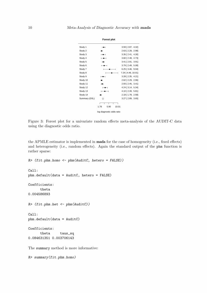
Note the sensitivity and false positive rate returned in this summary are just the back-transformed µ1 and µ2. One can then proceed to plot the SROC curve of this model. Bydefault the point estimate of the pair of sensitivity and false positive rate is also plotted to-gether with a confidence region. In the following example the SROC curve is plotted a bitthicker using the sroclwd argument, a caption is added to the plot and also the data and alegend. By default the SROC curve is not extrapolated beyond the range of the original data:

R> plot(fit.reitsma, sroclwd = 2,

+ main = "SROC curve (bivariate model) for AUDIT-C data")


0.0 0.2 0.4 0.6 0.8 1.0

0.0

0.2

0.4

0.6

0.8

1.0

SROC curve (bivariate model) for AUDIT−C data

False Positive Rate

Sen

sitiv

ity

●

●

datasummary estimate

SROCconf. region

Figure 5: SROC curve for the Reitsma et al. (2005) model.

R> points(fpr(AuditC), sens(AuditC), pch = 2)

R> legend("bottomright", c("data", "summary estimate"), pch = c(2,1))

R> legend("bottomleft", c("SROC", "conf. region"), lwd = c(2,1))

The output is shown in Figure 5.

6.1. Comparing SROC curves

We show how to compare SROC curves. Patrick, Cheadle, Thompson, Diehr, Koepsell, andKinne (1994) conducted a meta-analysis to (among other things) investigate the efficacy ofself administered and interviewer administered questionnaires to detect nicotine use. Thedata sets SAQ and IAQ are the respective subsets of this data. First one fits bivariate modelsto the data sets:

R> data("IAQ")

R> data("SAQ")

R> # both datasets contain more than one 2x2-table per study

R> # reduce (somewhat arbitrarily) to one row per study by

R> # using the first coded table only:

R> IAQ1 <- subset(IAQ, IAQ$result_id == 1)

R> SAQ1 <- subset(SAQ, SAQ$result_id == 1)

R> fit.IAQ <- reitsma(IAQ1)

R> fit.SAQ <- reitsma(SAQ1)

Then one plots the SROC curves of these fits, beginning with the fit of the IAQ and addingthe SAQ curve. Note that the lty arguments is used so that the curves can be distinguished.


0.0 0.1 0.2 0.3 0.4 0.5

0.5

0.6

0.7

0.8

0.9

1.0

Comparison of IAQ and SAQ

False Positive Rate

Sen

sitiv

ity

●

●

●

●

●

● ●

●

●

●

● ●

●

●

● ●

● ●

●

●

● IAQSAQ

Figure 6: Comparison of interviewer and self-adminstered smoking questionaires with SROCcurves.

R> plot(fit.IAQ, xlim = c(0,.5), ylim = c(.5,1),

+ main = "Comparison of IAQ and SAQ")

R> lines(sroc(fit.SAQ), lty = 2)

R> ROCellipse(fit.SAQ, lty = 2, pch = 2, add = TRUE)

R> points(fpr(IAQ1), sens(IAQ1), cex = .5)

R> points(fpr(SAQ1), sens(SAQ1), pch = 2, cex = 0.5)

R> legend("bottomright", c("IAQ", "SAQ"), pch = 1:2, lty = 1:2)

Figure 6 contains the resulting plot. The summary estimates are well separated, though theconfidence regions slightly overlap. It would nevertheless be safe to conclude that IAQ is amore reliable way to measure smoking than SAQ.

6.2. Bivariate meta-regression

We demonstrate diagnostic meta-regression also using the data of Patrick et al. (1994). Weuse the complete data set, which is loaded by

R> data("smoking")

R> # again reduce to one result per study:

R> smoking1 <- subset(smoking, smoking$result_id == 1)

The data.frame contains the same variables as the SAQ and IAQ subsets, but the type iscoded by the variable type:

R> summary(smoking1$type)

IAQ SAQ

10 16


We use the factor type as a covariate in diagnostic meta-regression:

R> fit.smoking.type <- reitsma(smoking1,

+ formula = cbind(tsens, tfpr) ~ type)

Note that the left hand side of the formula object always has to be of the form cbind(tsens,

tfpr), where tsens and tfpr are for transformed sensitivity and false positive rate respec-tively. We generate detailed output by:

R> summary(fit.smoking.type)

Call: reitsma.default(data = smoking1, formula = cbind(tsens, tfpr) ~

type)

Bivariate diagnostic random-effects meta-analysis

Estimation method: REML

Fixed-effects coefficients

Estimate Std. Error z Pr(>|z|) 95%ci.lb

tsens.(Intercept) 2.813 0.491 5.735 0.000 1.852

tsens.typeSAQ -1.166 0.634 -1.838 0.066 -2.409

tfpr.(Intercept) -3.337 0.311 -10.733 0.000 -3.946

tfpr.typeSAQ 0.882 0.389 2.269 0.023 0.120

95%ci.ub

tsens.(Intercept) 3.775 ***

tsens.typeSAQ 0.077 .

tfpr.(Intercept) -2.727 ***

tfpr.typeSAQ 1.645 *

---

Signif. codes: 0 '***' 0.001 '**' 0.01 '*' 0.05 '.' 0.1 ' ' 1

Variance components: between-studies Std. Dev and correlation matrix

Std. Dev tsens tfpr

tsens 1.508 1.000 .

tfpr 0.875 0.551 1.000

logLik AIC BIC

70.721 -127.441 -113.783

This output can be interpreted as follows: The z value for the regression coefficient for thesensitivities is significant, indicating that the interviewer administered questionnaires offer abetter sensitivity. Interestingly the point estimate for the false-positive rates does not indicateany effect.

Note that once meta-regression is used, one cannot reasonably plot SROC curves, since fixedvalues for the covariates would have to be supplied to do so. Also (global) AUC values do notmake sense.


We can also compare the fit of two bivariate meta-regressions with a likelihood-ratio test. Forthis, we have to refit the models with the maximum likelihood method, as the likelihood-ratiotest relies on asymptotic theory that is only valid if this estimation method is employed.

R> fit.smoking.ml.type <- reitsma(smoking1,

+ formula = cbind(tsens, tfpr) ~ type,

+ method = "ml")

R> fit.smoking.ml.intercept <- reitsma(smoking1,

+ formula = cbind(tsens, tfpr) ~ 1,

+ method = "ml")

R> anova(fit.smoking.ml.type, fit.smoking.ml.intercept)

Likelihood-ratio test

Model 1: cbind(tsens, tfpr) ~ type

Model 2: cbind(tsens, tfpr) ~ 1

ChiSquared Df Pr(>ChiSquared)

13.25 2 0.00133 **

---

Signif. codes: 0 '***' 0.001 '**' 0.01 '*' 0.05 '.' 0.1 ' ' 1

The meta-regression confirms that type explains some of the heterogeneity between the pri-mary studies.

6.3. Transformations beyond the logit

All bivariate approaches explained so far use the conventional logit transformation. Thereitsma function offers the parametric tα family (Doebler et al. 2012) of transformations asalternatives. The family is defined by

tα(x) := α log(x)− (2− α) log(1− x), x ∈ (0, 1), α ∈ [0, 2].

For α = 1, the logit is obtained. In many cases the fit of a bivariate meta-regression can beimproved upon by choosing adequate values for α. The rational behind this is, that especiallysensitivities tend to cluster around values like .95 and the symmetric logit transformationdoes not necessarily lead to normally distributed transformed proportions. As an example westudy the smoking data again using maximum-likelihood estimation:

R> fit.smoking1 <- reitsma(smoking1, method = "ml")

R> fit.smoking2 <- reitsma(smoking1,

+ alphasens = 0, alphafpr = 2,

+ method = "ml")

R> AIC(fit.smoking1)

[1] -120.0473

R> AIC(fit.smoking2)


[1] -120.1002

The almost identical AIC values indicates, that the fit of the models is comparable. Forpurpose of inference, we likelihood-ratio tests are recommended, which are discussed for thistype of transformation by Doebler et al. (2012).

7. Further development

In the future mada will support the mixture approach of Holling, Bohning, and Bohning(2012a) and Bayesian approaches.

Acknowledgements

This work was funded by the DFG project HO 1286/7-2.

References

Arends L, Hamza T, Van Houwelingen J, Heijenbrok-Kal M, Hunink M, Stijnen T (2008).“Bivariate Random Effects Meta-Analysis of ROC Curves.” Medical Decision Making, 28,621–638.

Biostat, Inc (2006). “Comprehensive Meta-Analysis (CMA), Version 2.” Computer program.

Borenstein M, Hedges L, Higgins J, Rothstein H (2009). Introduction to Meta-Analysis. JohnWiley & Sons.

Cochran W (1954). “The Combination of Estimates from Different Experiments.” Biometrics,10, 101–129.

Deeks J (2001). “Systematic Reviews of Evaluations of Diagnostic and Screening Tests.”British Medical Journal, 323, 157–162.

DerSimonian R, Laird N (1986). “Meta-Analysis in Clinical Trials.” Controlled Clinical Trials,7, 177–188.

Doebler P, Holling H, Bohning D (2012). “A Mixed Model Approach to Meta-Analysis ofDiagnostic Studies With Binary Test Outcome.” Psychological Methods.

Gasparrini A, Armstrong B, Kenward MG (2012). “Multivariate Meta-Analysis for Non-Linear and other Multi-Parameter Associations.” Statistics in Medicine, Epub ahead ofprint(doi: 10.1002/sim.5471).

Gatsonis C, Paliwal P (2006). “Meta-Analysis of Diagnostic and Screening Test AccuracyEvaluations: Methodologic Primer.” American Journal of Roentgenology, 187, 271–281.

Glas A, Lijmer J, Prins M, Bonsel G, Bossuyt P (2003). “The Diagnostic Odds Ratio: ASingle Indicator of Test Performance.” Journal of Clinical Epidemiology, 56, 1129–1135.


Harbord R, Deeks J, Egger M, Whiting P, Sterne J (2007). “A Unification of Models forMeta-Analysis of Diagnostic Accuracy Studies.” Biostatistics, 8, 239–251.

Harbord R, Whiting P (2010). “metandi: Meta-Analysis of Diagnostic Accuracy Using Hier-archical Logistic Regression.” Stata Journal, 9, 211–229.

Higgins J, Thompson S, Deeks J, Altman D (2003). “Measuring Inconsistency in Meta-Analyses.” British Medical Journal, 327, 557–560.

Holling H, Bohning W, Bohning D (2012a). “Likelihood-Based Clustering of Meta-AnalyticSROC Curves.” Psychometrika, 77, 106–126.

Holling H, Bohning W, Bohning D (2012b). “Meta-Analysis of Diagnostic Studies Basedupon SROC-Curves: A Mixed Model Approach Using the Lehmann Family.” StatisticalModelling, 12, 347–375.

Jones C, Athanasiou T (2005). “Summary Receiver Operating Characteristic Curve AnalysisTechniques in the Evaluation of Diagnostic Tests.” The Annals of Thoracic Surgery, 79,16–20.

Kriston L, Holzel L, Weiser A, Berner M, Harter M (2008). “Meta-Analysis: Are 3 QuestionsEnough to Detect Unhealthy Alcohol Use?” Annals of Internal Medicine, 149, 879–888.

Le C (2006). “A Solution for the Most Basic Optimization Problem Associated with an ROCCurve.” Statistical Methods in Medical Research, 15, 571–584.

Leeflang M, Deeks J, Gatsonis C, Bossuyt P (2008). “Systematic Reviews of Diagnostic TestAccuracy.” Annals of Internal Medicine, 149, 889–897.

Lunn D, Spiegelhalter D, Thomas A, Best N (2009). “The BUGS Project: Evolution, Critiqueand Future Directions.” Statistics in Medicine, 28(25), 3049–3067.

Lunn D, Thomas A, Best N, Spiegelhalter D (2000). “WinBUGS – a Bayesian ModellingFramework: Concepts, Structure, and Extensibility.” Statistics and computing, 10, 325–337.

Patrick D, Cheadle A, Thompson D, Diehr P, Koepsell T, Kinne S (1994). “The Validity ofSelf-reported Smoking: A Review and Meta-Analysis.” American Journal of Public Health,84, 1086–1093.

Phillips B, Stewart L, Sutton A (2010). “Cross Hairs Plots for Diagnostic Meta-Analysis.”Research Synthesis Methods, 1, 308–315.

R Core Team (2012). R: A Language and Environment for Statistical Computing. R Foun-dation for Statistical Computing, Vienna, Austria. ISBN 3-900051-07-0, URL http:

//www.R-project.org/.

Reitsma J, Glas A, Rutjes A, Scholten R, Bossuyt P, Zwinderman A (2005). “Bivariate Anal-ysis of Sensitivity and Specificity Produces Informative Summary Measures in DiagnosticReviews.” Journal of Clinical Epidemiology, 58, 982–990.

Rutter C, Gatsonis C (2001). “A Hierarchical Regression Approach to Meta-Analysis ofDiagnostic Test Accuracy evaluations.” Statistics in Medicine, 20, 2865–2884.

http://www.R-project.org/

http://www.R-project.org/


Sutton A, Abrams K, Jones D, Sheldon T, Song F (2000). Methods for Meta-Analysis inMedical Research. John Wiley & Sons.

Takwoingi Y, Deeks J (2011). “METADAS: An SAS Macro for Meta-Analysis of DiagnosticAccuracy Studies, Version 1.3.” Computer program.

The Nordic Cochrane Centre (2011). “Review Manager (RevMan), Version 5.1.” Computerprogram.

Van Houwelingen H, Arends L, Stijnen T (2002). “Advanced Methods in Meta-Analysis:Multivariate Approach and Meta-Regression.” Statistics in Medicine, 21, 589–624.

Walter S (2002). “Properties of the Summary Receiver Operating Characteristic (SROC)Curve for Diagnostic Test Data.” Statistics in Medicine, 21, 1237–1256.

Affiliation:

Philipp DoeblerFachbereich Psychologie und SportwissenschaftWestfalische Wilhelms-Universitat MunsterD-48149 Munster, GermanyE-mail: [email protected]: http://wwwpsy.uni-muenster.de/Psychologie.inst4/AEHolling/personen/P_Doebler.html

Heinz HollingFachbereich Psychologie und SportwissenschaftWestfalische Wilhelms-Universitat MunsterD-48149 Munster, GermanyE-mail: [email protected]: http://wwwpsy.uni-muenster.de/Psychologie.inst4/AEHolling/personen/holling.html

mailto:[email protected]

http://wwwpsy.uni-muenster.de/Psychologie.inst4/AEHolling/personen/P_Doebler.html

http://wwwpsy.uni-muenster.de/Psychologie.inst4/AEHolling/personen/P_Doebler.html

mailto:[email protected]

http://wwwpsy.uni-muenster.de/Psychologie.inst4/AEHolling/personen/holling.html

http://wwwpsy.uni-muenster.de/Psychologie.inst4/AEHolling/personen/holling.html

Documents

Meta-Analysis of Diagnostic Accuracy with mada · 2019-09-27 · Meta-Analysis of Diagnostic Accuracy with mada Philipp Doebler WWU M unster Heinz Holling WWU M unster Abstract The