Page 1 of 53

Mesoscale-duration activated states gate spiking in response to fast rises in 1 membrane voltage in the awake brain 2

3

AUTHORS 4

Annabelle C. Singer1,2*, Giovanni Talei Franzesi2*, Suhasa B. Kodandaramaiah2,3, Francisco J. Flores4, 5 Jeremy D. Cohen5, Albert K. Lee5, Christoph Borgers6, Craig R. Forest7, Nancy J. Kopell8, Edward S. 6 Boyden2+ 7

8

AFFILIATIONS 9

1Coulter Department of Biomedical Engineering, Georgia Institute Of Technology and Emory University, 10 Atlanta, GA, USA. 11

2Media Lab, McGovern Institute for Brain Research, Departments of Biological Engineering and Brain 12 and Cognitive Sciences, Massachusetts Institute of Technology, Cambridge, MA, USA. 13

3Department of Mechanical Engineering, University of Minnesota, Twin Cities, Minneapolis, MN, USA. 14

4Brain and Cognitive Sciences, Massachusetts Institute of Technology, Cambridge, MA, USA and 15 Department of Anesthesia, Critical Care and Pain Medicine, Massachusetts General Hospital and Harvard 16 Medical School, Boston, MA, USA. 17

5Howard Hughes Medical Institute, Janelia Research Campus, Ashburn, VA, USA 18

6Department of Mathematics, Tufts University, Medford, MA, USA. 19

7George W. Woodruff School of Mechanical Engineering, Georgia Institute Of Technology, Atlanta, GA, 20 USA. 21

8Department of Mathematics and Statistics, Boston University, Boston, MA, USA. 22

23

24

ADDITIONAL FOOTNOTES 25

*These authors contributed equally to this work. 26

27

Articles in PresS. J Neurophysiol (May 31, 2017). doi:10.1152/jn.00116.2017

Copyright © 2017 by the American Physiological Society.

Page 2 of 53

RUNNING TITLE 28

Mesoscale activated states gate spiking in the awake brain 29

KEYWORDS 30

Network state; CA1, hippocampus; barrel cortex; intracellular recording; action potential; subthreshold 31 dynamics 32

ADDRESS FOR CORRESPONDENCE 33

+Correspondence to: 34

Edward Boyden 35 Departments of Biological Engineering and Brain and Cognitive Sciences 36 Massachusetts Institute of Technology 37 E15-421, 20 Ames St., Cambridge, MA 02139 38 email - esb@media.mit.edu 39 phone - (617) 324-3085 40

ABSTRACT 41

Seconds-scale network states, affecting many neurons within a network, modulate neural activity by 42

complementing fast integration of neuron-specific inputs that arrive in the milliseconds before spiking. 43

Non-rhythmic subthreshold dynamics at intermediate timescales, however, are less well-characterized. 44

We found, using automated whole cell patch clamping in vivo, that spikes recorded in CA1 and barrel 45

cortex in awake mice are often preceded not only by monotonic voltage rises lasting milliseconds, but 46

also by more gradual (lasting 10s-100s of ms) depolarizations. The latter exert a gating function on 47

spiking, in a fashion that depends on the gradual rise duration: the probability of spiking was higher for 48

longer gradual rises, even controlling for the amplitude of the gradual rises. Barrel cortex double-49

autopatch recordings show that gradual rises are shared across some but not all neurons. The gradual rises 50

may represent a new kind of state, intermediate both in timescale and in proportion of neurons 51

participating, which gates a neuron's ability to respond to subsequent inputs. 52

53

Page 3 of 53

54

NEW AND NOTEWORTHY 55

We analyzed subthreshold activity preceding spikes in hippocampus and barrel cortex of awake mice. 56

Aperiodic voltage ramps extending over 10s to 100s of milliseconds consistently precede and facilitate 57

spikes, in a manner dependent on both their amplitude and their duration. These voltage ramps represent 58

a “mesoscale” activated state that gates spike production in vivo. 59

INTRODUCTION 60

A wide variety of discrete or slowly varying (i.e., over timescales of seconds) neural network states have 61

been observed in the living mammalian brain, with many neurons in the network participating (Haider et 62

al., 2006; McGinley et al., 2015b, 2015a; Reimer et al., 2014; Steriade et al., 1993, 2001; Zagha and 63

McCormick, 2014). Fast dynamics occurring over timescales of a few to ten milliseconds have also been 64

studied in their relationship to spike generation and timing within single neurons (Azouz and Gray, 2000, 65

2008; Mainen and Sejnowski, 1995; Nowak et al., 1997; Pouille and Scanziani, 2001; Poulet and Petersen, 66

2008). In between such slow and fast timescale events, there has been much interest in oscillations with 67

periods in the tens to hundreds of milliseconds (e.g. (Başar et al., 2001; Buzsáki and Draguhn, 2004; Fries, 68

2009; Klimesch, 1999; Singer, 1993). 69

An open question is whether there are other stereotyped forms of dynamics that help shape neural activity 70

over intermediate timescales. We intracellularly recorded, in awake mice, spontaneous activity in the 71

CA1 field of the hippocampus and in the barrel cortex, and discovered that most spikes were preceded by 72

membrane voltage rises lasting tens to hundreds of milliseconds. Such voltage rises did not, however, 73

exhibit apparent periodicity, in contrast to the oscillatory dynamics often studied over such timescales. 74

Page 4 of 53

We characterized these intermediate duration (or mesoscale) rises in the mouse barrel cortex using 75

simultaneous dual whole cell patch clamp (which can be performed in surface structures by our multi-76

neuron autopatching system), and found that, for any pair of neurons, they occurred in a coordinated 77

fashion at least part of the time, suggesting that they are shared by time-varying subsets of neurons within 78

the network. Thus, these mesoscale rises in membrane voltage appear to represent a novel activated state, 79

intermediate both in timescale and in the proportion of neurons participating, to classical slowly varying 80

states and fast single neuron dynamics. These mesoscale voltage rises exerted a gating function on 81

subsequent inputs, in the sense that neurons were more likely to spike in response to an endogenous fast 82

rise in voltage, or to a brief near-threshold injected current, if it was preceded by a mesoscale rise. 83

Moreover, mesoscale rises did not simply increase the probability of spiking by depolarizing the cell 84

because the duration of the mesoscale rise also affected spike probability: brief current pulses delivered 85

during mesoscale rises had significantly higher probability of resulting in a spike than pulses delivered 86

during shorter depolarizing events that reached the same pre-stimulus membrane voltage. This suggests 87

that single-cell, in addition to network-level, effects can play an important role in how such membrane 88

voltage dynamics shape neuronal output. Such intermediate activated states may facilitate neural 89

processing by boosting the probability that a neuron might respond to a weak input, as occurs in many 90

sensory and cognitive processes. Our results also demonstrate the new kinds of findings that can be 91

revealed with awake autopatching and multineuron autopatching in vivo. 92

MATERIALS AND METHODS 93

Surgical procedures 94

All animal procedures were approved by the MIT Committee on Animal Care. Adult male C57BL/6 mice 95

(Taconic) 8-12 weeks old were anesthetized using isoflurane and placed in a stereotactic frame. The scalp 96

was shaved, ophthalmic ointment (Puralube Vet Ointment, Dechra) was applied to the eyes, and Betadine 97

and 70% ethanol were used to sterilize the surgical area. Three self-tapping screws (F000CE094, Morris 98

Page 5 of 53

Precision Screws and Parts) were attached to the skull, target craniotomy sites were marked on the skull 99

(in mm, from bregma: 2 A/P, -1.4 M/L for the whole-cell recording site in CA1 and -3.23 A/P, -0.58 M/L 100

for the local field potential (LFP) electrode site in CA1, 1 A/P, -2.8 M/L; 1 A/P, -3.2 M/L; 1.5 A/P, -2.8 101

M/L and 1.5 A/P, -3.2 M/L for multiple whole-cell recording sites in barrel cortex), and a custom stainless 102

steel (for hippocampal recordings on the spherical treadmill) or delrin (for barrel cortex recordings in non-103

running mice) headplate was affixed using dental cement (C&B Metabond, Parkell). 104

On the day of the experiment, a dental drill was used under isoflurane anesthesia to open one to four 105

craniotomies (200-400 µm diameter) by first thinning the skull until ~100 µm thick, and then using a 30 106

gauge needle to make a small aperture. The craniotomy was then sealed with a sterile silicone elastomer 107

(Kwik-Sil WPI) until recording. Animals were then allowed to wake up from anesthesia. 108

Behavior training and virtual reality environment (VR) 109

For CA1 recordings, the headfixed animals ran on an 8” spherical treadmill as described in Harvey et al. 110

(Harvey et al., 2009). For 16 out of 18 analyzed CA1 cells, animals ran on the spherical treadmill in a 111

dimly lit room; for 2 cells animals ran in a virtual reality environment. For virtual reality environment 112

recordings, the motion of the spherical treadmill was measured by an optical mouse and fed into virtual 113

reality software (Aronov and Tank, 2014) running in MATLAB (version 2013b, Mathworks). The virtual 114

environment consisted of a linear track with two small enclosures at the ends where the animal could turn. 115

Animals received a reward of sweetened condensed milk diluted 1:2 in water from a spout at each end of 116

the track after visiting the other end. 117

Animals learned to run on the track over approximately one week. The animals were left to recover from 118

the surgery for one week and habituated to handling for one to two days before behavioral training began. 119

To acclimate to the testing environment, on the first two days of training the animals were placed on the 120

spherical treadmill with the VR system off and were rewarded with undiluted sweetened condensed milk. 121

Page 6 of 53

From the third day until the end of training (typically 5-7 days) the animals were placed on the treadmill 122

for increasing amounts of time (30 minutes to 2 hours) running in the VR linear track. Animals were 123

rewarded with diluted (1:2) sweetened condensed milk at the end of the linear track after traversing the 124

length of the track. 125

Awake immobilized set up and habituation 126

For cortical recordings, the animals were affixed in a custom head and body restraint setup similar to that 127

described by Guo et al. (Guo et al., 2014). The mice were allowed to recover for 10 days after surgical 128

implantation of headplates prior to habituation to the recording setup. Habituation was carried out for 6 129

consecutive days with training sessions lasting 30 to 60 minutes on each day. The animals were given 130

undiluted condensed milk at 10-15 minute intervals during the habituation sessions. 131

Electrophysiology reagents 132

For whole-cell patching, borosilicate glass pipettes (Warner) were pulled using a micropipette puller 133

(Flaming-Brown P97 or P2000 models, Sutter Instruments) from capillaries with 0.69 mm and 1.2 mm 134

internal and outer diameters, respectively. We pulled glass pipettes with resistances between 4-9 MΩ and 135

with an approximate outer diameter of ~300-400 µm at a point 1.5 mm from the tip in order to minimize 136

tissue displacement and to allow for the use of small craniotomies. The intracellular pipette solution 137

consisted of (in mM): 125 potassium gluconate (with more – an additional 0 – 25 mM -- added 138

empirically to bring the solution to ~290 mOsm; pH was 7.2), 0.1 CaCl2, 0.6 MgCl2, 1 EGTA, 10 HEPES, 139

4 Mg ATP, 0.4 Na GTP, 8 NaCl. For biocytin staining, 500 μM of biocytin, sodium salt (Invitrogen) was 140

added to the pipette solution. The LFP electrode was pulled from quartz capillaries with internal and outer 141

diameters of 0.3 and 1 mm, respectively, on a pipette puller (P2000, Sutter Instruments) to a fine tip, 142

which was then manually broken back to a diameter of ~10µm. For recording, the LFP electrode was 143

filled with sterile saline. 144

Page 7 of 53

Mapping the target locations in CA1 145

Electrodes were positioned to advance through the whole-cell recording site craniotomy parallel to the 146

coronal plane and perpendicular to the horizontal plane and to advance through the LFP recording site 147

craniotomy at an angle 60 degrees posterior to the coronal plane and 45 degrees inferior to the horizontal 148

plane. The LFP electrode was slowly advanced into the brain until clear electrophysiological signatures of 149

the hippocampal stratum pyramidale (str. pyr.) layer were observed (~600-1000 µV theta waves while the 150

animal was running, clearly distinguishable sharp-wave ripples during immobility, multiple spikes greater 151

than 50 µV, Fig. 1A,B), then retracted 25-50 µm in order to make room for safe positioning of the patch 152

pipette. A similar procedure was followed to map the putative location of the str. pyr. through the 153

craniotomy to be used for whole-cell patching. Although the geometrical arrangement of the two 154

electrodes was calculated to place them within 500 µm of each other, to further ensure that both LFP and 155

whole-cell recordings were taken from the same region of CA1, we simultaneously recorded the LFP at 156

both locations and calculated the cross-correlation between the two signals at the beginning of the first 157

recording day (Fig. 1A,C). The pipettes were considered adequately co-localized if the cross-correlation 158

at zero lag was above 0.85, and if, by visually inspecting the two simultaneous traces, we could confirm 159

that the peaks and troughs of theta and gamma oscillations and of sharp-wave ripples were aligned within 160

~1 ms of each other (Fig. 1C). Further validation of the electrode locations was done post-mortem, by 161

either biocytin filling of patched cells or dye injection (AlexaFluor 594 and AlexaFluor 488, Molecular 162

Probes, Fig. 1A, D). 163

Awake autopatcher hardware and operation 164

The awake autopatcher employed in our experiments was a modification of the one described in 165

Kodandaramaiah et al. (Kodandaramaiah et al., 2012). A custom-built pressure control system was used 166

to apply positive and negative pressure to the pipette (see http://autopatcher.org). The hardware was 167

controlled by custom software written in Labview (National Instruments). 168

Page 8 of 53

The autopatching algorithm was modified from that use in anesthetized animals to compensate for 169

increased brain motion in awake animals. Up to the stage of gigaseal formation the robot followed the 170

algorithm described in (Kodandaramaiah et al., 2012), with the following changes: (1) switching to an 171

intermediate pressure (300-800 mbar) 100 µm above the target region to minimize damage to the area of 172

interest, (2) advancing through the brain more slowly (2 µm steps at 1µm/s) to give the tissue time to 173

relax, and (3) increasing the number of samples over which to calculate resistance and using a modified 174

threshold for cell detection (a resistance increase of 250 kΩ over three steps or 400 kΩ over five steps, 175

with an increase of at least 50 kΩ per step) to account for movement-induced variability in the awake 176

brain. 177

Gigaseal formation followed the same procedure as (Kodandaramaiah et al., 2012), but was sped up to 178

prevent a detected cell from moving away from the pipette due to brain motion. In addition if the 179

resistance did not increase rapidly enough (greater than 10 MΩ/s) the robot either applied additional 180

periods of gentle suction, moved forward 1-6 µm, and/or further hyperpolarized the pipette (up to a 181

maximum of -90 mV). The experimenter could also manually complete patching if needed. 182

Once a seal was formed (typically between 800 MΩ and several GΩ) the experimenter switched the 183

program to break-in mode and either sequences of suction (-150 to -250 mbar) pulses or continuous low (-184

20 to -30 mbar) suction were applied until whole-cell access was achieved. 185

In addition to the changes described, keeping the craniotomy size less than 300 μm and using very long 186

shanked pipettes, to reduce tissue damage and tissue relaxation, were also important to maximize yield. 187

The updated software for awake autopatching will be uploaded to http://autopatcher.org at time of 188

publication. Access resistances were 37.9±14.6 MΩ and membrane resistances were 93.3±56.9 MΩ 189

(mean ± standard deviation). Neurons were recorded for 16.1±13.4 min (N = 61 neurons) (see Review-190

only Fig. 1A). We did not record total recording duration or membrane parameters for all neurons. 191

Page 9 of 53

Neurons were excluded from subsequent analysis if the simultaneous LFP recording was absent or 192

contaminated by high frequency artifacts, if the neuron did not spike at any point during the recording, or 193

if the neuron’s firing rate was above 4 Hz (see Inclusion criteria below). 194

Autopatching of two neurons 195

We used four autopatchers (Kodandaramaiah et al., 2012, 2016) at once to control up to four patch 196

pipettes simultaneously within a single cortical microcircuit. Pipettes were angled at 45 degrees from 197

vertical and arranged symmetrically around the craniotomies in a circle with 90 degrees between each 198

pipette; pipettes were 45 degrees from the animal’s midline. Pipettes were positioned in the craniotomies 199

such that their tips entered and converged to a 200-300 µm wide region.. The robot lowered all the 200

pipettes to the target depth (350-650 µm targeting layers 2/3, 4 and 5) and checked them for tip fouling or 201

blockage. The robot then moved all good pipettes in small steps (2-3 µm), until a pipette detected a 202

neuron, whereupon the robot halted the movement of all pipettes and attempted to establish a gigaseal in 203

the channel(s) that had encountered a neuron. After gigasealing was complete (or failed), the motor for 204

that channel was deactivated, and the rest of the pipettes resumed neuron hunting. This process was 205

repeated until all the pipettes had encountered neurons and attempted gigasealing. At this point, the 206

channels that had successfully formed gigaseals were selected and the robot applied pulses of suction to 207

break into the cells for whole cell recordings. The updated software for using multiple autopatchers at 208

once will be uploaded to http://autopatcher.org at time of publication. Access resistances were 31.2±15.5 209

MΩ and membrane resistances were 103.9±79.3 MΩ (mean ± standard deviation). Cells were recorded 210

for 39.6±24.6 min. (N = 38 neurons). Neurons were excluded from subsequent analysis if they did not 211

spike at any point during the recording or if the neuron’s firing rate was above 4 Hz (see Inclusion 212

criteria). 213

Data acquisition 214

Page 10 of 53

Data was acquired with a sampling rate of 20kHz. Local field potentials were recorded simultaneously 215

with the whole-cell data at 20kHz, and bandpass filtered 1Hz-1kHz. At the beginning of whole cell 216

recording depolarizing square wave current pulses were delivered to measure membrane resistance, 217

access resistance, and the membrane time constant (see Review-only Fig. 1A and 3A for access 218

resistance values). During some recordings, a sequence of current pulses of increasing amplitude was 219

delivered to characterize the neuron’s response properties (see e.g. (Andersen, 2007)). Whole cell 220

recordings in current clamp mode then commenced. Some cells were injected with a small amount of 221

current (0 to -100pA) during the experiment (Epsztein et al., 2011). 222

We typically recorded multiple cells per animal in a session. To avoid having multiple biocytin-filled cells 223

and to reduce background staining, we only added biocytin to pipettes to fill neurons towards the end of 224

the recording session. 225

Recording sessions were terminated after approximately 3 hours for immobilized mice and 5 hours for 226

behaving mice. 227

Experimental Procedures for Data Contributed by J.D.C. and A.K.L. 228

Surgery 229

Three eight-to-twelve week-old male C57BL/6NCrl (Charles River Laboratories) mice were used for 230

these experiments. All procedures were performed in accordance with the Janelia Research Campus 231

Institutional Animal Care and Use Committee guidelines on animal welfare. Prior to behavioral training, a 232

stainless steel head plate – with a large central recording well to access the hippocampus bilaterally – was 233

attached to the skull surface using light-cured adhesives (Optibond All-in-One, Kerr; Charisma, Heraeus 234

Kulzer) and dental acrylic. Sites for future hippocampal CA1 craniotomies (bregma: -1.6 to -2.0 mm AP, 235

1.2 to 1.8 mm ML) were marked with a fine-tipped cautery pen (Medline). Mice were allowed to recover 236

for at least five days before behavioral training started. During recovery, the mice were given food and 237

Page 11 of 53

water ad libitum. 238

Behavioral Setup and Training 239

The day before starting behavioral training, mice were placed on water-restriction (1.0 ml/day). Body 240

weight and overall health were checked each day to ensure the mice remained healthy over the course of 241

the experiment (Guo et al., 2014). On day 1, the head was centered and fixed atop a large spherical 242

treadmill (http://www.flintbox.com/public/project/26501/), with the eyes ~20 mm from the surface. 243

Animals received artificially sweetened water rewards (acesulfame potassium, 4 mM, Sigma-Aldrich; ~2 244

µl liquid drop per reward). Motion of the treadmill was tracked using a two-camera system (modified 245

from https://openwiki.janelia.org/wiki/display/flyfizz/Home; Seelig et al., 2010). Over a period of 10 days, 246

mice were trained to explore a variety of visual-based virtual reality mazes (software was developed at the 247

HHMI Janelia Research Campus as part of Janelia’s open-source virtual reality software platform, Jovian). 248

Rewards were earned as the mice completed laps around the virtual environments. 249

Electrophysiology 250

On recording days (≥ day 11), mice were anesthetized with isoflurane (~1.5%, ~0.8 l/min flow rate), 251

placed in a stereotaxic frame, and a craniotomy (~ 1 mm2) was performed over dorsal CA1. A glass 252

recording pipette (~2 MΩ) filled with saline was lowered into the brain and used to monitor the 253

extracellular local field potential and unit activity in order to accurately map the depth of the dorsal CA1 254

pyramidal cell layer. After a minimum of 1 h post-surgery recovery time, mice were placed on the 255

treadmill. Blind in vivo whole-cell recordings were obtained from the right or left dorsal CA1 pyramidal 256

cell layer (Lee et al., 2009; Lee et al., 2014) using recording pipettes (5-7 MΩ) filled with an intracellular 257

solution containing (in mM) K-gluconate 135, HEPES 10, Na2-phosphocreatine 10, KCl 4, MgATP 4, and 258

Na3GTP 0.3 (pH adjusted to 7.2 with KOH) as well as biocytin (0.2%). After achieving the whole-cell 259

configuration, the VR display was turned on and the mice were free to explore the mazes for sweetened 260

Page 12 of 53

water rewards. Current-clamp measurements of Vm (amplifier low-pass filter set to 5 kHz) were sampled 261

at 25 kHz. All data analyzed is from recording periods with no holding current applied to the pipette. 262

Recordings were not corrected for the liquid junction potential. All neurons contributed had the 263

electrophysiological characteristics of somatic CA1 pyramidal whole-cell recordings (Lee et al., 2009; 264

Lee et al., 2014). 265

Analysis of whole cell recordings 266

Inclusion criteria 267

All recorded intracellular traces were visually inspected and only traces with a stable baseline with an 268

average membrane voltage less than -45 mV and spike amplitude greater than 40 mV were included. Cells 269

recorded from CA1 were also excluded if the simultaneously recorded local field potential showed 270

electrical artifacts (e.g. 60 Hz noise). We recorded 22 cells in CA1 and 25 cells in barrel cortex that 271

reached these criteria for inclusion. Of the 25 cells recorded in barrel cortex, eight cells were from paired 272

recording when two cells were recorded simultaneously. To examine the ramp-up in voltage preceding 273

spiking, we initially restricted the analysis to spikes that occurred at least 300 ms after a prior spike, to 274

ensure that the ramp from baseline to spike threshold was not obscured by prior spikes. We subsequently 275

repeated the analysis including spikes that occurred at least 100 ms after a prior spike, though we 276

excluded cases when the cell did not return to baseline between spikes (e.g., bursting), obtaining 277

quantitatively similar results (see Review-only Supp. Results). 278

The majority of the cells we recorded from had low mean firing rates (less than 4 Hz) including all but 279

two cells in CA1 and one cell in barrel cortex. We excluded cells that had fewer than five spikes that fit 280

our criteria for inclusion (see above). As a result 15 cells in CA1 and 22 cells in barrel cortex were 281

included for the single cell analyses (details on paired recordings are described below). In these cells, 282

more than half the spikes on average occurred at least 300 ms after a prior spike (55.13% ± 27.27% of 283

Page 13 of 53

spikes in 15 cells in CA1 and 61.11% ± 22.88% in 22 cells in barrel cortex, mean ± standard deviation). 284

Greater than two-thirds of the spikes on average occurred at least 100 ms after a prior spike (66.92% ± 285

26.49 of spikes in CA1 and 68.30% ± 23.22 of spikes in barrel cortex). 286

Spike threshold calculation 287

In vivo, because the membrane voltage and conductance are constantly changing, spike threshold can vary 288

by as much as 5-10 mV (Azouz and Gray, 2000, 2003; Henze and Buzsaki, 2001). As a result, in vivo 289

spike threshold is often measured as the voltage reached at spike initiation, which is thought to occur at 290

the inflection point in the membrane voltage before the spike peak (Bean, 2007). To identify this 291

inflection point, we used increases in the second derivative, specifically when the second derivative 292

reached greater than four standard deviations above the mean. This definition of spike threshold was used 293

for all analysis, unless otherwise noted. To confirm the robustness of our findings we also used a second 294

definition: the highest membrane potential in the trace not associated with a spike (see Review-only Fig. 295

2A, B and 3D, E), similar to the approach in Fontaine et al. (Fontaine et al., 2014). This was calculated 296

by finding all the times when the membrane potential went above baseline for at least 20 ms and returned 297

to baseline without spiking and calculating the maximum voltage during all of those periods. We called 298

this latter method the alternate method for determining spike threshold. 299

Determining the start of the ramp-up 300

The start of the ramp-up in voltage preceding spikes was identified as the point when the membrane 301

potential went above and stayed above the smoothed membrane potential until spike threshold (computed 302

as described in the Spike threshold calculation section). The smoothed membrane potential was computed 303

by first replacing spikes in the trace with a linear interpolation over four milliseconds before and seven 304

milliseconds after the spike peak, and smoothing the resulting trace with a ten second wide Gaussian filter. 305

This produced an average of the trace without spikes that can track slow changes in voltage. We will refer 306

Page 14 of 53

to this smoothed membrane potential as the baseline, for simplicity. We found quantitatively similar 307

results if we calculated a mean baseline (the mean of the whole trace after spikes were thus removed, data 308

not shown) instead of a smoothed membrane potential. The vast majority of the time, when the membrane 309

potential went above baseline it peaked or reached spike threshold within 400 ms, therefore we excluded 310

rare outliers when the membrane potential did not peak or reach spike threshold within this period. 311

Spike burst analysis 312

For spike burst analysis we selected spikes which were followed by another spike within 10 ms, a time 313

window consistent with burst firing (see Review-only Fig. 1B, 3C). In hippocampus, 8 cells had both 314

single spikes and spikes separated from the next spike by less than 10ms. In barrel cortex, 15 cells had 315

both single spikes and spikes separated from the next spike by less than 10ms. We found quantitatively 316

similar results when we considered cases with a second spike within 50 ms (data not shown). 317

Bimodality of membrane potential traces 318

Hartigan’s dip statistic, for which higher values indicate more bimodal distributions, was used to quantify 319

membrane voltage bimodality. Based on visual inspection of the distributions, distributions with a 320

Hartigan’s dip statistic less than 0.0005 were considered more unimodal, greater than 0.001 were 321

considered more bimodal, and between 0.0005 and 0.001 were considered in between for purposes of 322

separately plotting these distributions. 323

Fast rise analysis 324

Fast, monotonic rises in membrane potential preceding spikes (see review-only Supp. Table 1 for number 325

of spikes included in the analysis) were calculated from the time when the slope of the membrane 326

potential became and stayed positive until spike threshold (computed as described in the Spike threshold 327

calculation section), meaning the membrane potential rose monotonically during that period. This 328

Page 15 of 53

definition was used for the fast rise analyses in Fig. 4A-D, 5C, 7D-F, review-only Fig. 2, 3D-G, and 4G-329

I. To compute the slope, the despiked trace (spikes were removed and linearly interpolated over from 330

threshold to seven milliseconds after the spike peak to fully remove the spike waveform) was first 331

smoothed with a three millisecond wide Gaussian filter and then the change in voltage over each point in 332

time (dV/dt) was computed. A three millisecond Gaussian was chosen for smoothing the trace before 333

computing the slope because we found this best matched our aim of minimal smoothing that would 334

reduce noise in the slope while accurately preserving the changes in the raw trace. Note that while such 335

smoothing reduces our temporal resolution at durations less than three milliseconds long, we were not 336

aiming to characterize dynamics in the membrane potential significantly faster than this. The size and 337

duration of the fast rise in voltage preceding spikes was measured from the start of this positive slope. 338

Spikes for which the fast rise in membrane potential started at or below baseline were considered to not 339

have a gradual rise in membrane potential before threshold. Spikes that had no consistent increase in 340

membrane potential (positive slope) before the spike were considered to have no fast rise in membrane 341

potential before threshold. 342

Comparison of gradual rises and other long-lasting depolarizations. 343

We computed the size and duration of ramp-ups above baseline that did or did not result in spikes. First 344

we identified depolarizing events when the membrane potential went and stayed above baseline for at 345

least 20 ms to extract periods of depolarization that were longer than most fast rises in voltage. Then we 346

measured the size and duration of the ramp-up from the start of these depolarizing events to their peak if 347

there was no spike or to spike threshold of the first spike during the event. Spikes that did not fall into one 348

of these depolarizing events (e.g. spike threshold was at or below baseline) were rare and were excluded. 349

We then separated ramp-ups in depolarizing events into gradual rises and fast rises and measured the 350

change in voltage and duration of each of these components. The end of the gradual rise and beginning of 351

Page 16 of 53

the fast rise in voltage was identified as when the slope of the membrane potential became positive and 352

stayed positive until the peak of the event or until spike threshold. 353

Assessing gradual rises periodicity 354

To determine if gradual rises that tend to precede spikes were periodic, we measured the interval between 355

them. To examine the periodicity of gradual rises that were similar to the depolarizing events preceding 356

spikes, we only included those (with or without spikes) that were longer and larger than the bottom 25% 357

of gradual rises of depolarizing events with spikes. We repeated this analysis only including gradual rises 358

that were longer and larger than the bottom 50% of gradual rises preceding spikes and found similar 359

results (data not shown). 360

Current injection experiments 361

We injected in 6 CA1 neurons short current pulses of varying amplitudes so as to obtain recordings in 362

which the neurons had either a low (1.5-3.7%), a medium (12-27%), or a high (37-61%) probability of 363

firing in response to the pulses. We analyzed the probability of the neurons firing in response to the 364

stimulus as a function of the presence or absence of a gradual rise immediately preceding the current 365

pulse (where ‘gradual rise’ is defined as a depolarization with duration and amplitude falling within the 366

20th-80th percentiles of gradual rises recorded before endogenous spikes). To analyze whether gradual 367

rises affected spike probability exclusively by bringing the membrane voltage closer to spike threshold, or 368

whether the temporal aspect of gradual rises also mattered, for each set of recordings (with low, medium, 369

or high overall spike probability) we sorted the stimulus pulses depending on the size of the preceding 370

depolarization (1-2, 2-5, 5-7 mv) and its duration (0-10 ms and 50-200 ms). We only analyzed conditions 371

for which >3 pulses were present and the amplitude of the pre-stimulus depolarization was not 372

significantly different (p > 0.05) for the 0-10ms and 50-200ms categories (see Review-only Supp. Table 1 373

for details). Qualitatively similar results were obtained when analyzing the data grouping the recordings 374

Page 17 of 53

by different criteria (e.g. amplitude of evoked depolarization), having different categories for pre-stimulus 375

depolarization amplitude (e.g. 1-3, 3-10 mV) and duration (e.g. 3-13 ms, 33-95 ms). 376

Spike probability as a function of gradual and fast rises duration and amplitude 377

We binned the data by the duration or amplitude of the gradual rise and the duration or amplitude of the 378

fast rise in voltage. For each bin, we computed the proportion of all the depolarizing events that had 379

spikes to determine the probability of spiking as a function of the gradual rise and fast rise amplitude and 380

duration. We computed the proportion of events with spikes per cell and then took the average of all cells 381

(see Review-only Supp. Table1 for number of depolarizing events with and without spikes per cell in 382

CA1 and barrel cortex). Only bins that included data from at least three cells were included. 383

Monotonic increases in membrane potential properties and spiking probability 384

We defined monotonically increasing events as events when the slope of the membrane potential became 385

and stayed positive for at least 3 ms, to identify periods that were about the length of, or longer than, most 386

monotonic increases preceding spikes. Then we measured the size and duration to the peak of events 387

without a spike or to spike threshold of events with a spike. As we did for the depolarizing events with 388

spikes, we computed the proportion of monotonically increasing events with spikes as a function of the 389

change in voltage and duration to the peak or spike threshold. We computed the proportion of events with 390

spikes per cell and then took the average of all cells (see Review-only Table 1 for number of 391

monotonically increasing events with and without spikes in CA1 and barrel cortex). Only bins that 392

included data from at least three cells were included. 393

Generalized linear models 394

To examine how the duration of the gradual rise contributed to the probability of spiking, we used a 395

generalized linear model (GLM) (Nelder and Wedderburn, 1992)) . We first generated a logistic binomial 396

Page 18 of 53

model of the probability of spiking as a function of duration of the gradual rise alone. In this model the 397

probability of a spike, p, was the dependent variable. The probability was predicted based on the gradual 398

rise durations of depolarizing events. Because the distribution of the dependent variable was binomial 399

(either there was a spike in a depolarizing event or there was not) we used a binomial link function. This 400

model is a binomial version of regression and uses the following formula, which is the canonical linking 401

function for a binomial dependent variable: 402

log(p/(1-p)) = b0 + b1X1 403

where p is the probability of a spike, X1 is the duration of the gradual rise, b0 is the intercept, and b1 is the 404

coefficient of X1. The GLM estimates b0 and b1 (the residuals) and yields T values and p-values for those 405

estimates that can be used to evaluate the probability that the duration of the gradual rise predicts the 406

probability of a spike. 407

408

We looked for influential outliers using Cook’s distance (Fox, 2008) (10-20 points that had Cook’s 409

distances of ~0.01-0.7 which were above the other points; Cook’s distance values closer to one are more 410

likely to be outliers). Initially, we found some outliers, which upon closer inspection were data points 411

with long ramp-ups (>~400 ms). We therefore decided to exclude cases with these extra-long ramp-ups 412

(>300 ms). To make sure that the model was not driven by a small subset of influential points, we 413

randomly selected half of the data and estimated the regressors with each half of the data separately. The 414

estimates were very similar in both cases (see Review-only material for details). 415

416

We then aimed to estimate the probability of spiking as a function of both the duration and size of the 417

gradual rise. To do this we fit a logistic binomial model of the probability of spiking as a function of 418

duration of the gradual rise, the change in voltage during the gradual rise, and the interaction between 419

these factors using the following linking function 420

log(p/(1-p)) = b0 + b1X1 + b2X2 + b3X1*X2 421

Page 19 of 53

where p is the probability of a spike, X1 is the duration of the gradual rise, X2 is the change in voltage 422

during the gradual rise, b0 is the intercept, b1 is the coefficient of X1, b2 is the coefficient of X2, and b3 is 423

the coefficient of the interaction between X1 and X2. Again we looked for influential outliers using Cook’s 424

distance and found a few outliers (1-5 points that had Cook’s distances of ~0.005-0.04 that were above 425

the other points). These were all data points with larger gradual rises (>~18 mV in CA1 and >~26 mV in 426

barrel cortex). We therefore decided to exclude cases with larger gradual rises (>16 mV in CA1 and >24 427

mV in barrel cortex). For Cook’s distance, all values were less than 0.01 for single cell analyses and less 428

than 0.025 for paired cell analyses. 429

Dual intracellular recordings analysis 430

The single cell analyses included four pairs of simultaneously recorded cells. To further examine 431

simultaneous intracellular activity, we recorded from additional cell pairs for a total of seven cell pairs in 432

barrel cortex for which both cells reached criteria for inclusion (see Inclusion criteria section). 433

In these cells we detected depolarizing events as we did for single cells. For each depolarizing event, we 434

computed the Pearson’s correlation coefficient between the membrane potential of the cells from the start 435

of the depolarizing event until the peak of the event (if there was no spike), or until spike threshold (if 436

there was a spike). We measured the duration and amplitude of these depolarizing events, as we did for 437

single cells, separating them into three groups: depolarizing events with a spike in the same cell used to 438

detect the depolarizing event, with a spike in the nearby neuron but not in the same cell, or without any 439

spikes in either cell. 440

We selected spikes from one cell in the pair (the reference spiking neuron) and compared the membrane 441

potential during the period preceding those spikes to the membrane potential of the other cell in the pair 442

(the nearby neuron). We then repeated these analysis selecting spikes (see section Inclusion criteria) from 443

the other cell in the pair, which would then be deemed the spiking neuron. 444

Page 20 of 53

Statistical analyses 445

We performed a Lilliefors test on each distribution to determine if it was normally distributed. When the 446

distributions were not normal we used appropriate nonparametric tests. When ranges of values are 447

reported they indicate 20-80th percentiles unless otherwise stated. 448

Analysis of local field potential and network state 449

To detect periods of theta oscillations, sharp-wave ripples (SWR), and periods outside of either network 450

state, the LFP was first downsampled to 2 kHz and bandpass filtered between 150 and 250 Hz. SWRs 451

were detected when the envelope amplitude of the filtered trace was greater than four standard deviations 452

above the mean for at least 15 ms. The envelope amplitude was calculated by taking the absolute value of 453

the Hilbert transform of the filtered LFP. Spikes that occurred during the SWR and during the 250 ms 454

before and after the ripples were classified as SWR spikes because population spiking related to SWRs 455

(such as replay events) often extends before and after the SWR itself (Davidson et al., 2009; Dragoi and 456

Tonegawa, 2011). To detect theta, the LFP was bandpass filtered for theta (4-12 Hz), delta (1-4 Hz), and 457

beta (12-30 Hz) using an FIR equiripple filter. The ratio of theta to delta and beta (‘theta ratio’) was 458

computed as the theta envelope amplitude divided by the sum of the delta and beta envelope amplitudes. 459

Theta periods were classified as such when the theta ratio was greater than one standard deviation above 460

mean for at least one second and the ratio reached a peak of at least two standard deviations above mean. 461

SWRs and theta periods thus classified where further checked by visual inspection. 462

We then examined the ramp-up to spikes that occurred during theta periods, sharp wave ripple periods, or 463

outside these periods. Twelve cells had spikes during both sharp wave ripple periods and non-theta, non-464

sharp wave ripple periods. Seven cells had spikes during both theta periods and non-theta, non-sharp 465

wave ripple periods. 466

Mathematical model describing spike probability as a function of ramp-up duration 467

Page 21 of 53

Assume that ramps of an arbitrary but fixed amplitude are of random duration, that spikes occur only 468

during an ongoing ramp, and that spikes are triggered by additional random excitatory inputs arriving on a 469

Poisson schedule with exponentially distributed inter-arrival times > 0 with the Poisson schedule 470

independent of the absence or presence of a ramp. Assume further that a spike terminates a ramp (as this 471

is how ramps were analyzed in the experimental data; it is difficult to analyze the ramp beyond a spike 472

due to active conductances engaged by the spike process, so this assumption may not be correct), but that 473

the ramp can also end without a spike. 474

475

We denote by T the random duration of a ramp that ends by itself, without a spike, and assume that T is 476

exponentially distributed with mean E(T) > 0. We denote by T the random duration of a ramp that ends 477

either spontaneously or with a spike, whichever occurs first: T = min (T, τ). Elementary probability 478

theory tells us that T is exponentially distributed with mean E(T ) = 1 E(T) + 1 E(τ) . Using 479

elementary arguments (see Appendix) the conditional probability that a ramp ends with a spike, given that 480

its duration T equals T (for a given T > 0), can be shown to equal E(TR)/E(τ), independently of T . 481

Written as a formula: 482

P(ramp ends in a spike|T = T ) = E(T )E(τ) . (1)

RESULTS 483

Long ramp-ups in voltage precede spikes in CA1 across network and behavior states 484

We recorded intracellularly from neurons in awake mice, using an awake mouse-optimized version of our 485

automated patch clamp robot (Kodandaramaiah et al., 2012, 2016). In neurons in hippocampal area CA1 486

(Fig. 2A, Review-only Fig 1A-B; N = 12 CA1 cells from 11 mice recorded while mice ran on a spherical 487

treadmill in a dimly lit room; 3 CA1 cells from 3 mice recorded while mice ran in on a spherical treadmill 488

in a virtual reality environment; see Methods) of awake mice, we observed that the majority of spikes 489

Page 22 of 53

were preceded by an extended ramp-up in voltage from baseline. These ramp-ups, measured for spikes 490

that occurred at least 300 ms after the previous spike (to standardize the analysis), lasted 31.20-114.45 ms 491

(20th-80th percentiles; median 57.65 ms; Fig. 2C,D; see Review-only Supp. Table 1 for number of spikes 492

per cell for all cell analyses) with 11.8% of the ramp-ups in CA1 neurons lasting over 150 ms. Similar 493

results were obtained when including spikes at least 100 ms after a prior spike: ramp-ups from baseline to 494

threshold lasted 26.28-138.76 ms (20-80th percentiles, median 52.50 ms for spikes that occurred 100-300 495

ms after a prior spike). We asked whether the long ramp-up might only occur in some specific cases, for 496

instance before spike bursts, but not before single spikes, since these spiking patterns may be generated by 497

different mechanisms (Grienberger et al., 2014). We therefore examined long ramp-ups preceding single 498

spikes versus multiple spikes (spikes that were followed by another spike within 10 ms, a time window 499

consistent with burst firing (Harris et al., 2001)). Spikes were preceded by long ramp-ups regardless of 500

whether they were isolated spikes or the first spike of a burst: ramp-ups preceding multiple spikes were 501

19.06-95.52 ms (20-80th percentiles, median 43.95) in duration and those preceding single spikes were 502

32.66-121.06 ms (20-80th percentiles, median 59.38) in duration. Although we found slightly shorter 503

duration ramp-ups preceding multiple spikes compared to single spikes, in CA1 these ramp-ups were not 504

significantly different when taking into account that multiple comparisons were performed (p-values: 505

0.5556, 0.6625, 0.1161, 0.0214, 0.7909, 0.1538, 0.5333, and 0.2075, ranksum test, Bonferroni corrected 506

p-value of 0.00625 for 8 CA1 cells that had both single and multiple spike events; N = 2-285 single spikes, 507

and 1-18 multiple spike events per cell 20th-80th percentiles, see Review-only Fig. 1B). 508

509

We then asked if long ramp-ups preceding spikes were unique to specific network states. Neural activity 510

across the hippocampal network changes markedly when animals run vs. sit quietly and these changes are 511

often referred to as different network states. These network states are clearly distinguishable by the 512

presence or absence of local field potential (LFP) oscillations in different frequency bands (Buzsáki, 513

2006; Buzsaki et al., 2003). In our experiments, mice ran on a spherical treadmill while we 514

Page 23 of 53

simultaneously whole cell patched neurons and recorded the extracellular local field potential to detect 515

changes in network state in CA1 (Fig. 1B). When animals ran, we observed large theta (6-12 Hz) 516

oscillations in CA1 as others have shown (Fig. 1B) (Buzsaki, 2002; Buzsaki et al., 2003; Harvey et al., 517

2009; Ravassard et al., 2013). When animals sat quietly, theta oscillations were no longer visible and we 518

recorded sharp wave ripples, high frequency oscillations of 150-250 Hz that last around 50-100 ms and 519

are associated with bursts of population activity, as others have observed (Fig. 1B) (Carr et al., 2011; 520

Foster and Wilson, 2006; Ylinen et al., 1995).Long ramp-ups preceded spikes during periods of theta 521

oscillations (see Methods and Fig. 1A,B), sharp-wave ripples (see Methods and Fig. 1A,B), or during 522

periods when neither theta nor sharp-wave ripples were detected (see Methods and Fig. 1A,B). For spikes 523

occurring during theta oscillations, ramp-ups started 32.85-94.26 ms before spike threshold (20th -80th 524

percentiles, median 67.90 ms, Fig. 2E,H and Supp. Results), during sharp-wave ripples ramp-ups started 525

36.89-116.21 ms before spike threshold (20th -80th percentiles, median 58.65 ms, Fig. 2F,I), and during 526

periods when neither theta nor sharp-wave ripples were detected ramp-ups started 30.78-113.83 ms before 527

spike threshold (20th -80th percentiles, median 56.208 ms, Fig. 2G, J and Supp. Results). Ramp-up 528

durations did not differ significantly between these states (Fig 2E-J). We correlated several measures 529

with the duration of the ramp-up in voltage preceding spikes. We found that in CA1 cells with larger 530

differences between baseline and threshold on average, cells with lower baseline membrane potential, or 531

cells with lower firing rates tended to have longer ramp-ups (Fig. 3A, Pearson's linear correlation 532

coefficient, start time of ramp-up vs threshold: r = -0.55, p = 0.033; vs mean baseline membrane potential: 533

r = 0.57, p = 0.028; vs. mean firing rate r = 0.60, p = 0.019, N = 15 cells in CA1). The durations of ramp-534

ups did not systematically depend the degree to which the membrane voltage was unimodal or bimodal 535

(see Methods, Fig. 3B). Thus, long ramp-ups occur, and exhibit similar properties, before spikes across a 536

wide variety of cellular and network states. The hippocampal cells recorded were most likely pyramidal 537

neurons, based on location (str. pyr.), low firing rate (Csicsvari et al., 1999; Hirase et al., 2001), and 538

morphological analysis of biocytin-filled cells (n = 3/3 pyramidal neurons). Since we typically recorded 539

Page 24 of 53

multiple cells per animal in a session, to avoid having multiple biocytin-filled cells and to reduce 540

background staining, we only added biocytin to pipettes to attempt to biocytin fill neurons towards the 541

end of the recording session, so that most cells recorded were not biocytin-filled. 542

543

Long ramp-ups can be decomposed into slow and fast components 544

Because in vitro, in vivo, and computational studies have suggested that the last approximately ten 545

milliseconds before a spike determine the precise timing of the spike (Azouz and Gray, 2000, 2008; 546

Mainen and Sejnowski, 1995; Nowak et al., 1997; Pouille and Scanziani, 2001) we examined whether a 547

fast component at this timescale could be identified within the ramp-up. We found that the ramp-ups 548

almost always ended in a monotonically increasing rise in membrane voltage that crossed spike threshold 549

(Fig. 4A), and developed a simple pipeline to quantify this visual observation. This ramp-up was quite 550

fast – 3.75-13.55 ms in duration (Fig. 4B 20th-80th percentile; median 7.40 ms). The preceding part of the 551

ramp-up before this fast rise we called the “gradual rise” (Fig. 4B), which lasted almost the entire 552

duration of the ramp-up: 22.1-105.18 ms, 20-80th percentiles (median 49.93 ms, 10.53% longer than 150 553

ms and 1.67% longer than 250 ms, N = 15 cells). Gradual rise durations could be calculated simply by 554

subtracting the durations of fast rises from the durations of overall long ramp-ups. 555

The majority of spikes were preceded by a gradual rise. Only 0.81% (median, 0-7.47% quartiles) of spikes 556

did not have a gradual rise and 0% (median, 0-0% quartiles, all but one cell was 0%) did not have a fast 557

rise (N = 15, Fig. 4D; for example traces see Review-only Fig. 2C), suggesting that both were needed to 558

effectively fire spikes. Importantly, the vast majority of fast rises started below spike threshold, showing 559

they are in fact a distinct component of subthreshold activity, rather than simply the initial component of 560

spikes. We compared the starting point of the fast rise to the spike threshold, calculated according to the 561

two spike threshold determination methods outlined in the Methods. The vast majority of the time the end 562

of the gradual rise was below both measures of threshold used: only 0.71% of spikes in CA1 and 1.79% in 563

Page 25 of 53

barrel cortex reached threshold, defined as when the second derivative reached greater than four standard 564

deviations above the mean (Azouz and Gray, 2000, 2008; Henze and Buzsaki, 2001), as a result of the 565

gradual rise alone (that is, the “fast rise” began after reaching spike threshold); only 0.08% of gradual 566

rises in CA1 and 1.52% of gradual rises in barrel cortex reached above the maximum membrane potential 567

not associated with a spike, the alternate threshold (Fontaine et al., 2014) we used. Therefore, we 568

conclude that the voltage at the start of the fast rise in voltage was below spike threshold. The gradual 569

rises and fast rises were similar in magnitude (Fig. 4C, 3.35-10.05 mV 20th-80th percentiles, median 6.69 570

mV for the gradual rise vs. 3.20-8.00 mV, 5.24 mV for the fast rise). These results held when analysis was 571

performed with an alternate definition of spike threshold (see Methods and Review-only Fig. 2A,B). 572

We conducted experiments in a laboratory outside of MIT to determine if long ramp-ups and their gradual 573

and fast components are present in CA1 neurons recorded by others under similar conditions (contributed 574

by authors J.D.C. and A.K.L., see Methods). We found the total ramp durations in these independently 575

recorded cells were qualitatively similar: 21.50 to 92.62 ms (20th-80th percentiles with a median 40.08 576

ms, Fig. 5A, B, N = 3 neurons (see Review-only Supp. Table 1 for number of spikes per cell)). As was 577

the case in our initial dataset, we also found these long ramp-ups contained gradual and fast rises that 578

were 14.28 to 87.40 ms gradual rises (median 36.84 ms) and 3.32 to 10.61 ms fast rises (median 6.72 ms, 579

Fig. 5C). These additional data independently validate the presence of long ramp voltage ramp-ups to 580

spiking with gradual and fast rise components. 581

582

Gradual rises preceding spikes are longer and larger than general fluctuations in the membrane potential 583

We next examined whether gradual rises that precede spikes exhibited different properties from other 584

long-lasting depolarizing events that do not precede spikes. We identified all of the periods where the 585

membrane potential of a neuron rose above baseline (see Methods for details) for at least 20 ms (a 586

duration longer than the 80th percentile of the fast rises, but shorter than the 20th percentile of the ramp-587

Page 26 of 53

ups), decomposing each such trace into a monotonic fast rise to its peak (for depolarizations without 588

spikes) or to spike threshold (for depolarizations with spikes), with the remaining part considered as the 589

gradual component. Gradual rises in voltage preceding spikes were longer (Fig. 4E, F, 26.19-113.24 ms 590

20th-80th percentiles, median 52.70 ms, for spike events, vs. 9.50-40.01 ms, median 18.35 ms for non-591

spike events; p < 10-50, ranksum test, N = 1087 spike events and 36217 non-spike events) and larger (Fig. 592

4G, 3.95-10.20 mV 20th-80th percentiles, median 6.98 mV, for spike events, vs. 0.99-4.11 mV and 2.21 593

mV for non-spike events; p < 10-50, ranksum test) than the gradual rises of depolarizing events that did not 594

result in spikes. 595

Gradual rises are not periodic nor do they have a signature in the local field potential 596

We aimed to determine if these gradual rises were related to oscillations (e.g. theta or slow oscillations), 597

or represented a new kind of aperiodic network phenomenon. We therefore measured the intervals 598

between the starts of gradual rises, because an interval measure reveals if an event is periodic regardless 599

of the shape of the trace and of whether the event repeats on every period or not. Because many of the 600

depolarizing events without spikes were short or small (see Fig. 4F, G distributions in blue) these small 601

short deviations above baseline could dominate the measure of intervals between gradual rises and might 602

mask any potential periodicity of the large gradual rises that preferentially lead to spikes. Therefore to 603

examine the periodicity of gradual rises that were similar to the depolarizing events preceding spikes, we 604

only included gradual rises of depolarizing events that were longer and larger than the bottom 25% of 605

gradual rises of depolarizing events with spikes (see Fig. 4F, G, 25% cut off from distribution in red but 606

gradual rises included from both distributions). We found a wide distribution of intervals between gradual 607

rise onsets (180.15 ms - 1.58 s, 20th -80th percentiles, median 547.15 ms) and while there was a slight 608

increase in gradual rise intervals between 50-200 ms, the majority of the intervals, 81%, fell outside this 609

range (Fig. 4H). We repeated this analysis only including depolarizing events with gradual rises that were 610

longer and larger than the bottom 50% of gradual rises preceding spikes and found similar results. We 611

Page 27 of 53

also examined the local field potential triggered from the start of these gradual rises and found no 612

signature in the local field potential to indicate extracellular oscillations (Fig. 4I). In all recordings (see 613

Methods) the distance between the two recording electrodes was less than 500 μm, and before each 614

recording session we recorded LFP from both the whole cell and LFP recording sites to confirm that the 615

LFPs were highly correlated across these locations. Recordings across both sites had a correlation 616

coefficient of at least 0.85 and theta oscillations, gamma oscillations, and sharp-wave ripples had peaks 617

that aligned within less than a millisecond (see Fig. 1B). Therefore differences between the intracellular 618

and LFP recordings were unlikely to be due to differences in recording location. Together these results 619

not only confirm the aperiodic nature of gradual rises, but additionally suggests that a smaller fraction of 620

neurons participate in a given gradual rise as compared to network states with a clear LFP signature. 621

Gradual rises gate spiking in response to subsequent inputs 622

To determine if monotonic increases in membrane potential alone were sufficient to determine when a 623

cell spiked, we identified monotonically increasing events and calculated the probability of spiking as a 624

function of their amplitude and duration (see Methods). Perhaps surprisingly, fast rises by themselves, 625

even when they were relatively large in amplitude, did not guarantee spiking (Fig. 6A), suggesting that 626

gradual rises might play a key role in spike generation. To test this in another way, we used the patch 627

pipette to deliver brief pulses of current to neurons in hippocampal CA1 (Fig. 6B, left). We delivered 628

these pulses at random times, and then post hoc analyzed the probability of neuron spiking as a function 629

of whether or not it was preceded by a gradual rise (defined as a depolarizing event having length and 630

duration in the upper 20th percentile of all depolarizing events in the population). We delivered currents 631

that resulted in, for the no-gradual rise case, a wide variety of voltage deflections and spike probabilities; 632

however, in all cases the presence of a gradual rise significantly enhanced the probability that the neuron 633

would spike in response to the stimulus (Fig. 6B, right; paired-sample t-test, p<0.01). Moreover, we 634

aimed to determine if the duration of the gradual rise preceding the pulse affected spike probability. To 635

Page 28 of 53

control for the size of the gradual rises, we grouped current pulses by both the size and duration of the 636

gradual rise preceding the pulse. We found the longer the cell had been depolarized (50-200ms compared 637

to 0-10ms), the higher the probability of spiking in response to the delivered current pulse, even for 638

gradual rises of similar size (Fig. 6C) (paired-sample t-test, p < 0.05). Note that there was a similar 639

distribution of gradual rise sizes between short and long ramp-ups in each group (see Review-only Supp. 640

Table 1). These results suggest that the duration, in addition to the amplitude, of the gradual rises is an 641

important aspect of how these rises affect neural function. Thus, gradual rises can indeed exert a causal 642

and facilitating role on spike generation, perhaps serving as an activated state for the neuron, boosting the 643

impact of subsequent fast events. 644

Long ramp-ups precede spikes in barrel cortex 645

We wondered if these long ramp-ups to spiking might be unique to the hippocampus or if they preceded 646

spikes in neurons of other circuits as well. To address this question, we performed whole-cell patch clamp 647

recordings from neurons in awake mouse barrel cortex and found similar long ramp-ups preceding spikes 648

(Fig. 7A,B,C; 36.10-149.00 ms, 20th-80th percentiles; median 72.55 ms; Review-only Fig. 3; N = 22 649

neurons from 15 mice which were awake, headfixed and immobilized, see Methods). Such long 650

membrane voltage ramp-ups occurred before both single and multiple spikes in the hippocampus: ramp-651

ups preceding multiple spikes were 24.90-93.63 ms (20-80th percentiles, median 51.45) in duration and 652

those before single spikes were 33.29-149.27 ms (median 71.00) in duration. Only one cell of fourteen 653

had significantly longer ramp-ups preceding bursts when taking into account that multiple comparisons 654

were performed (Review-only Fig. 3C, ranksum tests with p-values of 0.2485, 0.1058, 0.7514, 0.0069, 655

0.0035, 0.7464, 0.9247, 0.5035, 0.0046, 0.2805, 0.1176, 0.5505, 0.6667, and 0.4206 only one of which 656

was less than the Bonferroni corrected p-value of 0.0036 for N =14 cells in barrel cortex that had both 657

single and multiple spike events). We found similar results if we instead defined multiple spike events as 658

cases when the spike was followed by another spike within anywhere from 6-50 ms, to account for the 659

Page 29 of 53

possible differences between in vitro and in vivo preparations, animal models and recording techniques. 660

This strongly suggests that long ramp-ups consistently precede spikes across different spiking patterns, 661

rather than being restricted to either spike bursts or single spikes. 662

Average cell parameters (e.g. mean firing rate, mean change from baseline to threshold) were not 663

correlated with ramp-up duration (Fig. 8A, Pearson's linear correlation coefficient, start time of ramp-up 664

vs. mean change in membrane potential from baseline to threshold r = 0.18447, p = 0.42341; vs. mean 665

baseline membrane potential r = -0.12759, p = 0.58153; vs. mean firing rate r = 0.13176, p = 0.56915, N = 666

21 cells that had at least 3 spikes in barrel cortex). 667

We also examined histograms of the voltage difference from baseline to determine if the membrane 668

potential tended to be bimodal or unimodal. Many distributions were unimodal while some were bimodal 669

(Fig. 8B). We sorted the cells by the degree of bimodality or unimodality in their membrane voltage 670

distribution, measured using Hartigan’s dip statistic (Hartigan and Hartigan, 1985), and found no clear 671

relationship between the duration of the ramp-up and the degree of unimodality or bimodality of the trace 672

(Fig. 8B). 673

These ramp-ups in barrel cortex included a gradual rise which lasted most of the ramp-up followed by a 674

fast rise (Fig. 7D, 22.67-138.56 ms, 20-80th percentiles, median 62.4 ms, 17.57% longer than 150 ms and 675

5.73% longer than 250 ms; fast rise duration: 4.86-21.28 ms, 20th-80th percentile; median 10.48 ms, N = 676

22 cells) and the fast and gradual components were of similar size (Fig. 7E, 3.95-14.75 mV, 20th-80th 677

percentiles, median, 10.44 mV for the gradual rise vs. 3.33-13.77 mV, 6.54 mV for the fast rise). As in 678

CA1 most spikes were preceded by both gradual and fast rises: only 9.22% (median, 0-21.05% quartiles) 679

of spikes did not have a gradual rise and 0% (median, 0-0% quartiles, all but one cell was 0%) did not 680

have a fast rise (Fig. 7F, N=22). Furthermore depolarizing events with spikes had longer (Fig. 7G, H, 681

34.47-150.66 ms, median 72.00 ms, for spike events, vs. 11.00-62.67 ms, median 24.90 s, for non-spike 682

events; p < 10-50, ranksum test, N = 985 spike events and 14429 non-spike events) and larger gradual rises 683

Page 30 of 53

than depolarizing events without spikes (Fig. 7G,I; 6.91-165.32 mV and 11.33 mV, spike events, vs. 684

1.61-9.14 mV and 4.39 mV, non-spike events; p < 10-50, ranksum test). The gradual rises in barrel cortex 685

were also not periodic (Fig. 7J, gradual rise intervals were 273.90 ms - 2.02 s, 20th -80th percentiles, 686

median 774.88 ms). These results show that long ramp-ups, consisting of a gradual and fast rise, occur in 687

multiple brain regions. We found that, as for hippocampal CA1 neurons, fast rises, even large ones, were 688

generally unable to drive barrel cortex neurons to fire spikes (Fig. 7K). 689

Gradual rise properties predicts spiking 690

We analyzed the probability of spiking when properties of both the gradual rise and the fast rise were 691

considered together (Fig. 9A,C, see Review-only Supp. Table 1 for number of events per cell), in 692

recordings from both hippocampal area CA1 and barrel cortex. A diagonal pattern emerged: in general, 693

the larger or longer the gradual rise, the smaller and shorter the fast rise needed to produce a high 694

probability of spiking. To investigate the relationship between gradual rise duration and spike probability 695

in the experimental data, we used a generalized linear model (GLM, see Methods and Review-only 696

material). We found that in the experimental data, the longer the gradual rise, the higher the probability 697

of spiking (Fig. 9B, left, 9D, left). The GLM derived from experimental data predicted that spikes would 698

occur with a probability of 14.1-17.8% for CA1 neurons and 12.8-16.0% for barrel cortex neurons (95% 699

confidence bounds) for 150 ms gradual rises, with the probability almost tripling to 42.6-55.1% for CA1 700

and 31.1-42.0% for barrel cortex for 250 ms gradual rises. 701

702

This result may at first not seem very surprising, since one might expect longer rises to be of higher 703

amplitude, and one might expect higher amplitude rises to be more effective at promoting spiking. 704

Surprisingly, however, the correlation between gradual rise duration and spiking probability holds even 705

for a given maximal amplitude of the rise. In fact, including gradual rise amplitude in the model (Fig. 9B, 706

right; Fig. 9D, right) showed that spike probability was higher for longer duration gradual rises among 707

gradual rises of small and medium amplitude. For instance, a 250ms or longer gradual rise of small (4mV) 708

Page 31 of 53

amplitude was as predictive of a spike as a much larger (12 mV), shorter rise. This shows that spike 709

probability increases with gradual rise duration, as we also observed during artificial stimulation (Fig. 6C). 710

711

We asked whether this observation could be explained on purely statistical grounds, that is, whether it 712

would be true, for probabilistic reasons alone, that long ramps would be more likely to end in a spike than 713

short ones. A simple model (see Methods) showed that if the ramps simply allowed spiking to occur in 714

response to inputs by raising voltage closer to threshold (hence with constant efficacy regardless of 715

duration), and if the fast excitatory inputs received by the neuron are Poissonian, the probability of a ramp 716

ending in a spike would have to be independent of ramp duration, contrary to the results of the GLM. 717

718

Gradual rises are coordinated across cells while fast rises are cell specific 719

The lack of a clear LFP signature suggests that not all cells in the network receive inputs underlying the 720

gradual rises. To determine if these gradual rises are, however, coordinated across some fraction of the 721

cells, we used a four-channel version of our autopatcher to record pairs of neurons within 500 microns of 722

each other in the barrel cortices of awake mice. In seven pairs of neurons, we noted that when one neuron 723

spiked (denoted the “reference neuron”), its ramp-up in voltage was sometimes highly correlated with the 724

ramp-up of the other neuron (denoted the “nearby neuron”), whether the nearby neuron spiked or not. For 725

example, in one neuron (Fig. 10A), 47.6% of these events exhibited a correlation greater than 0.5, 726

whereas 12.02% of the events exhibited a correlation of less than -0.5. Thus, uncorrelated as well as 727

anticorrelated events could be observed (see the other 6 neuron pairs’ correlations in Review-only Fig. 728

4A-F), even in the same cell. Across all cell pairs, 7.27% of events were anti-correlated (i.e., with 729

correlation less than -0.5), with 6 out of the 7 cell pairs exhibiting at least some anti-correlated events. 730

Overall, this suggests that gradual rises are shared across subsets of neurons in a network. However, 731

neurons that exhibit high correlations at some times, can be uncorrelated at other times, so that the 732

Page 32 of 53

fraction of the network being in an activated states changed over time. 733

To compare ramp-ups between cells, we selected spikes from one cell in the pair (the reference spiking 734

neuron) and compared the membrane potential during the period preceding those spikes to the membrane 735

potential of the other cell in the pair (the nearby neuron). We then repeated these analysis selecting spikes 736

(see section Inclusion criteria) from the other cell in the pair, which would then be deemed the spiking 737

neuron. On the whole, the correlations in ramp-up were significantly larger during depolarizing events 738

that led to spiking in at least one neuron of the pair than in depolarizing events (i.e. periods when the 739

membrane voltage rose above baseline) that did not lead to spikes in either neuron (Fig. 10B; p = 0.00021 740

ranksum test; N = 6282 depolarizing events with no spikes in either neuron, 289 depolarizing events with 741

a spike in at least one neuron). These results show that gradual rises that lead to spikes are not only larger 742

and longer than those that do not lead to spikes, but they are also more coherent across the network, 743

providing further evidence of their identity as distinct neuronal states. To probe this further, we examined 744

whether it was even possible to predict the spiking of one neuron using only the duration of the gradual 745

rise exhibited by the other neuron. Perhaps surprisingly, using a generalized linear model as in Fig. 9B, D, 746

we found that gradual rises lasting 250 ms in one neuron were associated with the other neuron exhibiting 747

a 29.2% chance of spiking (Fig. 10C, left). Note that this ability to predict the spiking of one neuron, from 748

the gradual rises of the other, occurred to some extent even when the latter neuron was engaged in a 749

depolarizing event that did not contain or result in a spike. As before, small gradual rises that were of long 750

duration were as predictive as large gradual rises (Fig. 10C, right). 751

In more detail, we analyzed depolarizing events that did not contain a spike, but during which the other 752

neuron did spike (Fig. 10D, left, dotted red line). These possessed gradual rises that were also larger and 753

longer (29.49-161.37 ms 20th-80th percentiles, median 69.35 ms vs. 12.05-66.95 ms, 26.9 ms; p < 10-20, 754

ranksum test, smaller than Bonferroni corrected p-value of 0.017 for 3 comparisons, N = 5492 755

depolarizing events with no spikes in either neuron, 211 depolarizing events with no spikes in the current 756

Page 33 of 53

neuron but a spike in the nearby neuron) than depolarizing events during which neither neuron spiked 757

(Fig. 10D, left, blue line). Indeed, these gradual rises were comparable to those that did precede spikes 758

(Fig. 10D, left, red line, 38.08-170.03 ms 20-80th percentiles, median 89.10 ms; p = 0.0267, ranksum test, 759

greater than the Bonferroni corrected p-value of 0.017 for 3 comparisons, N= 263 depolarizing events 760

with a spike in the current neuron, 211 depolarizing events with no spikes in the current neuron but a 761

spike in the nearby neuron from 7 cell pairs in barrel cortex). The amplitudes of the gradual rises followed 762

a similar pattern (Fig. 10D, right), although the gradual rise was smaller in the cell that did not fire 763

(shown in Fig. 10F, Review-only Fig. 4H). 764

If the gradual rises indeed represent a form of brief activated state shared across subsets of neurons, the 765

ramp-ups (which, as defined above, include both the gradual rise and subsequent fast-rise components) 766

would be expected to begin relatively synchronously. To determine if this was the case, we computed the 767

start of the ramp-up in each cell based on when that cell’s membrane potential went and stayed above 768

baseline until spike threshold was reached in the spiking cell of the pair: 16.8% of ramp-ups started within 769

10 ms of each other, 36.0% started within 20 ms of each other, and start times were correlated (Fig. 10E p 770

<10-10, Pearson's linear correlation coefficient, r = 0.389, N = 249 spikes, see also Review-only Fig. 4G). 771

In contrast to the coordination of gradual rises across multiple neurons, fast rises were cell-specific: when 772

one neuron spiked and the other did not, the spiking neuron had a fast rise of amplitude 2.93-13.95 (20th-773

80th percentile; median 5.98), whereas in the non-spiking cell the change in voltage was essentially absent, 774

0-1.89 mV (20th-80th percentiles, median 0.06 mV, Fig. 10G, see also Review-only Fig. 4I). Thus, unlike 775

the shared gradual rises which appeared in multiple neurons in the network, fast rises may reflect inputs 776

specific to individual cells or small subsets of cells in the network. 777

If spiking was highly correlated across neurons, it would in principle be possible that gradual rises might 778

appear correlated simply because they preceded correlated spikes. However, consistent with what others 779

have reported (e.g., (Poulet and Petersen, 2008)), spiking rarely occurred within a short time window in 780

Page 34 of 53

both neurons of a recorded pair. Out of 7 pairs only one had spikes co-occurring within 50 ms across the 781

two cells. In general, spikes co-occurring within hundreds of milliseconds were few, and in our analysis 782

we therefore pooled all spikes (i.e., co-occurring as well as non-co-occurring). Analysis of cases in which 783

both cells spiked within 150 ms (Review-only Fig. 4G, H, I) showed the same qualitative pattern as over 784

the entire spike population. We also performed the same analysis including only cases when one cell 785

spiked but the other one did not and again obtained similar results (Fig. 10E, F, G). 786

Others have observed highly correlated membrane potentials across simultaneously recorded cells during 787

periods of quiescence lasting for seconds (Poulet and Petersen 2008, Lampl et al. 1999). During these 788

highly correlated states, prominent 3-5 Hz oscillations were also observed in membrane potential. We 789

wondered if the correlated ramp-ups we found could simply be a result of these highly correlated periods, 790

which might last for periods of time longer than the ramp-ups themselves. If that were the case we might 791

expect to see periods of correlated membrane potential flanking the ramp-ups. To determine if correlated 792

ramp-ups fell within such correlated network states, we analyzed membrane potential correlations during 793

the period immediately preceding spikes, both when ramp-ups occur (15-215 ms before the spike) and in 794

the preceding period before the ramp-up (an equivalent time period immediately beforehand). Comparing 795

highly correlated ramp-up periods (correlation >0.8) and decorrelated ramp-ups periods (correlation <0.2), 796

we found no significant difference in the membrane potential correlations immediately preceding those 797

ramp-up periods (p > 0.7 Kolmogorov-Smirnov test, Fig. 11A,B). Thus, highly correlated ramp-ups were 798

not simply part of longer periods of more highly correlated network states, though the ramp-ups could 799

potentially be part of shorter network-wide states. 800

DISCUSSION 801

We have shown, using an awake animal-optimized version of our previously published autopatching 802

robot (Kodandaramaiah et al., 2012, 2016), as well as using a four-patch version capable of recording 803

multiple cells at once, and recording in both the hippocampus and the barrel cortex of awake mice, that in 804

Page 35 of 53

both brain regions spikes are nearly always preceded by two distinct subthreshold voltage changes: a fast 805

(4-17 ms) monotonic rise in membrane voltage that brings the neuron above threshold, riding on top of a 806

slower (tens to hundreds of milliseconds) gradual depolarization from baseline. The amplitude of the 807

gradual voltage rises was ~3-10 mV, similar to other subthreshold events known to modulate spike 808

probability (Carandini and Ferster, 2000; Contreras and Palmer, 2003; Haider et al., 2007; Sanchez-Vives 809

and McCormick, 2000). In support of this hypothesis, we found that such depolarizing ramps facilitate 810

spike probability when assessed with brief current injections near threshold. Importantly, neurons were 811

much more likely to spike in response to a brief injected current if it was preceded by a gradual rise, and 812

the probability of spiking was higher for longer gradual rises compared to shorter rises that reached the 813

same pre-stimulus voltage above baseline. Therefore the correlation between ramp duration and increased 814

spike probability was not simply due to patterns of activity in the network that drive both spiking and long 815

ramp-ups. Instead long ramp-ups increase spike probability in a cell-specific manner. Using dual patch 816

recordings in the barrel cortex, we found that whereas the fast component was highly cell-specific, the 817

gradual component was shared across multiple neurons in the network. This correlation between cells 818

during gradual rises was not simply due to long periods of correlated activity across cells: we found 819

correlations between cells could change over the course of 100s of milliseconds and membrane potential 820

correlations during periods before correlated ramp-ups were similar to those before de-correlated ramp-821

ups. 822

In the hippocampus, where much work has focused on how neural codes are influenced by various 823

rhythms, these gradual rises occurred independently of behavioral state and LFP oscillatory state (e.g., 824

periods of theta or sharp-wave ripple), and were themselves aperiodic, suggesting that gradual rises were 825

not simply intracellular correlates of classical neural oscillations. Furthermore, there was no prominent 826

LFP signature associated with gradual rises, suggesting that the fraction of neurons engaged during such a 827

rise was potentially much lower than found in states (e.g., up/down states) associated with prominent LFP 828

events. Thus, gradual rises may represent a “mesoscale” activated state, with intermediate durations, and 829

Page 36 of 53

likely intermediate numbers of neurons, as compared to other states commonly studied that are present in 830

a variety of network and behavioral states, in multiple brain regions. In support of this, while we often 831

saw correlations between gradual rises across neurons in a simultaneously recorded pair in barrel cortex, 832

neurons’ membrane dynamics were often not correlated – or even anti-correlated (see Fig. 10A and 833

Review-only Fig. 4A-F, far right)– suggesting that the ensemble of neurons engaged by any one ramp 834

event is a fraction of the neurons in the microcircuit, and the ensemble engaged by a particular ramp event 835

can be dynamically selected. 836

Duration of the mesoscale activated states affects spiking probability independently of peak voltage 837

838

In both barrel cortex and hippocampus, the GLM model derived from the experimental data shows that, 839

for a given amplitude, spiking probability significantly increases with duration of the mesoscale activated 840

state. This is in contrast to what is shown from a simplified model, assuming exponentially distributed 841

gradual rise durations and fast inputs arriving on a Poisson schedule. Both single-neuron and network-842

level mechanisms could explain this unexpected finding. At the single neuron level, for example, the 843

relatively prolonged depolarization might prime the neuron to be more responsive to incoming inputs. 844

One possibility is that slow depolarization could enhance persistent sodium current, known to be present 845

in hippocampal and cortical pyramidal neurons (Crill, 1996), to augment depolarization upon synaptic 846

input (Schwindt and Crill, 1995; Stafstrom et al., 1982) Our finding could, in principle, also be explained 847

by postulating different combinations of gradual rise and fast input distributions. For example, this could 848

happen if the fast inputs do not, in fact, follow a Poisson schedule, but their instantaneous probability 849

increases as a function of time elapsed since the last one. One way to test this is to use exogenously 850

delivered stimuli, since they do not affect the probability and schedule of fast inputs received by the 851

neuron during a gradual rise. As shown in Fig. 6 the correlation between longer gradual rises and 852

increased firing probability is observed for such stimulation as well, suggesting that single-cell effects 853

Page 37 of 53

play an important role. While we can’t confirm the identity of every recorded cell, we expect almost all of 854

the recordings to have been made in pyramidal cells. Two cells in CA1 and three cells in barrel cortex 855

were filled with biocytin, as described in the Methods. In CA1 both cells were classified as pyramidal 856

cells (see e.g. Fig. 1D, left); and in barrel cortex two cells were classified as pyramidal cells (see e.g. Fig. 857

1D, right) and one cell as an interneuron based on the morphology of the biocytin stained neurons. This 858

was in line with our expectations, based on our prior recordings (Kodandaramaiah et al., 2012), and, for 859

the CA1 recordings, because we were specifically targeting the CA1 str. pyr. 860

861

Mesoscale activated states and previously reported subthreshold dynamics 862

Several studies have analyzed subthreshold dynamics around spikes, and across-cell coordination in 863

anesthetized animals (Chen and Fetz, 2005; Haider et al., 2010; Lampl et al., 1999) and in awake 864

preparations (Bennett et al., 2013; Poulet and Petersen, 2008). One key difference is that previous studies 865

have often focused on a very short time window (e.g. 20 ms) before the spike as being the prime 866

determinant of spike generation (Chen and Fetz, 2005; Poulet and Petersen, 2008), generally paying less 867

attention to the dynamics that brought the neuron from baseline to close to spike threshold. Yet, as we 868

have shown, such dynamics play an important role in gating neuronal output. When slower dynamics 869

have been discussed, these dynamics have mostly been characterized by their frequency content over 870

relatively extended periods of time and correlations between cells across these frequencies (Bennett et al., 871

2013; Haider et al., 2010; Poulet and Petersen, 2008; Yu and Ferster, 2010). This approach would not 872

detect how the correlation between subthreshold dynamics across neurons can evolve over short 873

timescales. Other previous studies have identified dynamic changes in membrane potential correlations 874

over the timescale of seconds (e.g. Lampl et al. 1999), but whether such changes also occurred at shorter 875

timescales had not, to the best of our knowledge, been investigated. We therefore suggest that a 876

complementary, fruitful approach is to consider the gradual depolarizations on the 50-200ms timescale 877

Page 38 of 53

here described as individual ‘mesoscale’ responsive, or activated states, shared by dynamically changing 878

subsets of neurons in a network. Overall, our findings fit within the general theme of a rich variety of 879

dynamics at multiple timescales emerging from many groups (Haider and McCormick, 2009) and 880

involving varying proportions of neurons within a network that jointly control spike generation in vivo. 881

We here bring into focus a set of neuronal states of intermediate durations and extent, which has hitherto 882

not been explicitly recognized. 883

Possible functional implications of mesoscale activated states 884

At a theoretical level, such mesoscale activated states may have several effects that could be tested in the 885

future using new technologies and specific behavioral contexts. While assessing the possible role of 886

mesoscale activated states in sensory responses was beyond the scope of the present paper, the scheme we 887

propose would be consistent with both the ability of neurons to respond rapidly to sensory stimulation 888

(because of the fast rise), and with the large variability of responses shown in vivo (because whether the 889

neuron fires in response to the fast barrage of inputs is determined by the presence or absence of a pre-890

existing gradual rise). 891

Moreover, cell ensembles are often thought of as cells that fire together within a tight time window, which 892

occur during many behavioral contexts and appear to reflect information highly relevant to the task at 893

hand. By firing together in a coordinated fashion, such ensembles could drive any downstream cells 894

receiving convergent input to fire more efficaciously (Börgers et al., 2005; Fries, 2009). Mesoscale 895

activated states might be a natural mechanism for facilitating the generation of such cell ensembles: 896

gradual rises would prime a set of cells over tens of milliseconds, so that when a network receives a 897

barrage of input, these cells would be more likely to spike together. 898

Behaviorally, by making cells more likely to fire in response to subsequent inputs, mesoscale activated 899

states could boost spiking to behaviorally relevant, but less salient, stimuli. Previous work has shown that 900

Page 39 of 53

spiking activity can increase during attention even in the absence of stimuli (Luck et al., 1997; Reynolds 901

et al., 2000; Sundberg et al., 2009). One possibility is that the attentional state may boost activity even in 902

the absence of stimuli because of such transient depolarizations as described here; cells that enter 903

mesoscale activated states would be perfectly poised to respond to stimuli, though also more likely to be 904

driven above threshold by noise. It has been shown that when saccades occur, the visual cortex exhibits a 905

transient increase in excitability (Rajkai et al., 2008) that lasts for a hundred milliseconds or so (as 906

assessed with extracellular recording), raising the question of whether mechanisms like those described in 907

our study may play a role. It may be of interest for future studies to explore the possible interactions 908

between such mesoscale states and other postulated attentional mechanisms, such as gamma oscillations 909

(Fries, 2009; Womelsdorf et al., 2006). 910

Potential Cellular and Molecular Mechanisms 911

Further studies are needed to elucidate the cellular and network mechanisms that generate the mesoscale 912

activated states described here, but a starting point might be to first assess whether they are generated by 913

any mechanisms engaged by, or similar to, those underlying classical oscillatory states. For example, up 914

and down states are thought to arise from recurrent excitation between interconnected pyramidal cells that 915

is controlled by feedback inhibition and that can have relatively rapid onset and offset as the network 916

makes a transition as a whole (McCormick et al., 2003). Such whole-network transitions are thought to 917

require a high level of interconnectivity, which might apply to the barrel cortex, but not CA1 (at least 918

considered in isolation), where connections between pyramidal cells are sparse (Shepherd, 2004). Indeed, 919

because the gradual rises were similar in appearance in two different brain regions, a tantalizing 920

hypothesis is that that there might be common cellular mechanisms at play in multiple distinct circuits. 921

Although the connectivity patterns of neurons in CA1 and barrel cortex differ significantly, they share an 922

inhibitory interneuronal circuit by which VIP+ interneurons inhibit pyramidal cell-targeting PV+ and 923

SOM+ interneurons, with the net effect that activating VIP+ interneurons disinhibits pyramidal cells in 924

Page 40 of 53

the network (Freund and Buzsáki, 1996; Freund and Gulyás, 1997; Markram et al., 2004; McBain and 925

Fisahn, 2001; Pi et al., 2013). Activating VIP+ interneurons in these circuits could result in the mesoscale 926

activated states here described. A number of studies have already shown that activating VIP+ interneurons 927

in this circuit enables neuromodulators and glutamatergic projections (e.g., from higher order cortical 928

regions) to drive local cortical depolarization (Fu et al., 2014; Lee et al., 2013; Pfeffer et al., 2013; Pi et 929

al., 2013), suggesting these interneurons might be a common effector mechanism modulating excitability. 930

In the future, the ability to map neural circuits with both microcircuit detail and long-range projection 931

capability (Chen et al., 2015; Petreanu et al., 2007), as well as new methods for intracellular recording or 932

imaging of subthreshold events in many cells at once (Chen et al., 2013), may enable investigations of 933

how the mesoscale events here described arise from neural circuits. 934

935

936

AUTHOR CONTRIBUTIONS 937

ACS and GTF designed experiments, developed experimental methods, collected data, analyzed data, 938

interpreted results and wrote manuscript. SBK designed experiments, developed experimental methods, 939

collected data, advised on data analysis, and wrote manuscript. FJF designed experiments, collected data, 940

and advised on data analysis. JDC and AKL contributed independently recorded data. CB interpreted 941

results and derived mathematical model. CRF developed experimental methods. NJK advised on data 942

analysis and interpreted results. ESB designed experiments, advised on data analysis, interpreted results, 943

and wrote manuscript. 944

945

Page 41 of 53

GRANTS 946

A.C.S. was funded by the MIT Intelligence Initiative. G.T.F. was funded by a Friends of the McGovern 947

Institute Fellowship. E.S.B. was funded by NIH Director's Pioneer Award 1DP1NS087724 and 948

Transformative Award 1R01MH103910-01, New York Stem Cell Foundation-Robertson Award, the 949

Cognitive Rhythms Collaborative funded by NSF DMS 1042134, and NIH grants 1R01EY023173, 950

1R01NS067199, and 1R01DA029639. C.B. and N.J.K. were funded by NIH grant 1R01 NS067199. The 951

authors would like to thank Sunanda Sharma, Melina Tsitsiklis, Ilya Kolb, Denis Bozic, and Sean Batir 952

for training animals and setting up the VR system. 953

954

REFERENCES 955

Andersen, P. (2007). The hippocampus book (Oxford ; New York: Oxford University Press). 956 Aronov, D., and Tank, D.W. (2014). Engagement of Neural Circuits Underlying 2D Spatial Navigation in 957 a Rodent Virtual Reality System. Neuron 84, 442–456. 958 Azouz, R., and Gray, C.M. (2000). Dynamic spike threshold reveals a mechanism for synaptic 959 coincidence detection in cortical neurons in vivo. Proc. Natl. Acad. Sci. 97, 8110–8115. 960 Azouz, R., and Gray, C.M. (2003). Adaptive Coincidence Detection and Dynamic Gain Control in Visual 961 Cortical Neurons In Vivo. Neuron 37, 513–523. 962 Azouz, R., and Gray, C.M. (2008). Stimulus-selective spiking is driven by the relative timing of 963 synchronous excitation and disinhibition in cat striate neurons in vivo. Eur. J. Neurosci. 28, 1286–1300. 964 Başar, E., Başar-Eroglu, C., Karakaş, S., and Schürmann, M. (2001). Gamma, alpha, delta, and theta 965 oscillations govern cognitive processes. Int. J. Psychophysiol. 39, 241–248. 966 Bean, B.P. (2007). The action potential in mammalian central neurons. Nat Rev Neurosci 8, 451–465. 967 Bennett, C., Arroyo, S., and Hestrin, S. (2013). Subthreshold Mechanisms Underlying State-Dependent 968 Modulation of Visual Responses. Neuron 80, 350–357. 969 Börgers, C., Epstein, S., and Kopell, N.J. (2005). Background gamma rhythmicity and attention in cortical 970 local circuits: A computational study. Proc. Natl. Acad. Sci. U. S. A. 102, 7002–7007. 971 Buzsaki, G. (2002). Theta oscillations in the hippocampus. Neuron 33, 325–340. 972 Buzsáki, G. (2006). Rhythms of the brain (Oxford ; New York: Oxford University Press). 973 Buzsáki, G., and Draguhn, A. (2004). Neuronal Oscillations in Cortical Networks. Science 304, 1926–974 1929. 975 Buzsaki, G., Buhl, D.L., Harris, K.D., Csicsvari, J., Czeh, B., and Morozov, A. (2003). Hippocampal 976 network patterns of activity in the mouse. Neuroscience 116, 201–211. 977 Carandini, M., and Ferster, D. (2000). Membrane potential and firing rate in cat primary visual cortex. J. 978 Neurosci. 20, 470–484. 979 Carr, M.F., Jadhav, S.P., and Frank, L.M. (2011). Hippocampal replay in the awake state: a potential 980 substrate for memory consolidation and retrieval. Nat Neurosci 14, 147–153. 981

Page 42 of 53

Chen, D., and Fetz, E.E. (2005). Characteristic Membrane Potential Trajectories in Primate Sensorimotor 982 Cortex Neurons Recorded In Vivo. J. Neurophysiol. 94, 2713–2725. 983 Chen, F., Tillberg, P.W., and Boyden, E.S. (2015). Expansion microscopy. Science 347, 543–548. 984 Chen, T.-W., Wardill, T.J., Sun, Y., Pulver, S.R., Renninger, S.L., Baohan, A., Schreiter, E.R., Kerr, R.A., 985 Orger, M.B., Jayaraman, V., et al. (2013). Ultrasensitive fluorescent proteins for imaging neuronal 986 activity. Nature 499, 295–300. 987 Contreras, D., and Palmer, L. (2003). Response to contrast of electrophysiologically defined cell classes 988 in primary visual cortex. J. Neurosci. 23, 6936–6945. 989 Crill, W.E. (1996). Persistent sodium current in mammalian central neurons. Annu. Rev. Physiol. 58, 990 349–362. 991 Csicsvari, J., Hirase, H., Czurkó, A., Mamiya, A., and Buzsáki, G. (1999). Oscillatory Coupling of 992 Hippocampal Pyramidal Cells and Interneurons in the Behaving Rat. J. Neurosci. 19, 274–287. 993 Davidson, T.J., Kloosterman, F., and Wilson, M.A. (2009). Hippocampal replay of extended experience. 994 Neuron 63, 497–507. 995 Dragoi, G., and Tonegawa, S. (2011). Preplay of future place cell sequences by hippocampal cellular 996 assemblies. Nature 469, 397–401. 997 Epsztein, J., Brecht, M., and Lee, A.K. (2011). Intracellular Determinants of Hippocampal CA1 Place and 998 Silent Cell Activity in a Novel Environment. Neuron 70, 109–120. 999 Fontaine, B., Pena, J.L., and Brette, R. (2014). Spike-threshold adaptation predicted by membrane 1000 potential dynamics in vivo. PLoS Comput Biol 10, e1003560. 1001 Foster, D.J., and Wilson, M.A. (2006). Reverse replay of behavioural sequences in hippocampal place 1002 cells during the awake state. Nature 440, 680–683. 1003 Fox, J. (2008). Applied Regression Analysis and Generalized Linear Models (SAGE Publications). 1004 Freund, T. f., and Buzsáki, G. (1996). Interneurons of the hippocampus. Hippocampus 6, 347–470. 1005 Freund, T.F., and Gulyás, A.I. (1997). Inhibitory control of GABAergic interneurons in the hippocampus. 1006 Can. J. Physiol. Pharmacol. 75, 479–487. 1007 Fries, P. (2009). Neuronal Gamma-Band Synchronization as a Fundamental Process in Cortical 1008 Computation. Annu. Rev. Neurosci. 32, 209–224. 1009 Fu, Y., Tucciarone, J.M., Espinosa, J.S., Sheng, N., Darcy, D.P., Nicoll, R.A., Huang, Z.J., and Stryker, 1010 M.P. (2014). A Cortical Circuit for Gain Control by Behavioral State. Cell 156, 1139–1152. 1011 Grienberger, C., Chen, X., and Konnerth, A. (2014). NMDA receptor-dependent multidendrite Ca(2+) 1012 spikes required for hippocampal burst firing in vivo. Neuron 81, 1274–1281. 1013 Guo, Z.V., Hires, S.A., Li, N., O’Connor, D.H., Komiyama, T., Ophir, E., Huber, D., Bonardi, C., 1014 Morandell, K., Gutnisky, D., et al. (2014). Procedures for Behavioral Experiments in Head-Fixed Mice. 1015 PLoS ONE 9, e88678. 1016 Haider, B., and McCormick, D.A. (2009). Rapid Neocortical Dynamics: Cellular and Network 1017 Mechanisms. Neuron 62, 171–189. 1018 Haider, B., Duque, A., Hasenstaub, A.R., and McCormick, D.A. (2006). Neocortical Network Activity In 1019 Vivo Is Generated through a Dynamic Balance of Excitation and Inhibition. J. Neurosci. 26, 4535–4545. 1020 Haider, B., Duque, A., Hasenstaub, A.R., Yu, Y., and McCormick, D.A. (2007). Enhancement of Visual 1021 Responsiveness by Spontaneous Local Network Activity In Vivo. J. Neurophysiol. 97, 4186–4202. 1022 Haider, B., Krause, M.R., Duque, A., Yu, Y., Touryan, J., Mazer, J.A., and McCormick, D.A. (2010). 1023 Synaptic and Network Mechanisms of Sparse and Reliable Visual Cortical Activity during Nonclassical 1024 Receptive Field Stimulation. Neuron 65, 107–121. 1025 Harris, K.D., Hirase, H., Leinekugel, X., Henze, D.A., and Buzsaki, G. (2001). Temporal interaction 1026 between single spikes and complex spike bursts in hippocampal pyramidal cells. Neuron 32, 141–149. 1027 Hartigan, J.A., and Hartigan, P.M. (1985). The Dip Test of Unimodality. Ann. Stat. 13, 70–84. 1028 Harvey, C.D., Collman, F., Dombeck, D.A., and Tank, D.W. (2009). Intracellular dynamics of 1029 hippocampal place cells during virtual navigation. Nature 461, 941–946. 1030

Page 43 of 53

Henze, D.A., and Buzsaki, G. (2001). Action potential threshold of hippocampal pyramidal cells in vivo 1031 is increased by recent spiking activity. Neuroscience 105, 121–130. 1032 Hirase, H., Leinekugel, X., Czurkó, A., Csicsvari, J., and Buzsáki, G. (2001). Firing rates of hippocampal 1033 neurons are preserved during subsequent sleep episodes and modified by novel awake experience. Proc. 1034 Natl. Acad. Sci. 98, 9386–9390. 1035 Kass, R.E., Eden, U., and Brown, E. (2014). Analysis of Neural Data (Springer New York). 1036 Klimesch, W. (1999). EEG alpha and theta oscillations reflect cognitive and memory performance: a 1037 review and analysis. Brain Res. Rev. 29, 169–195. 1038 Kodandaramaiah, S.B., Franzesi, G.T., Chow, B.Y., Boyden, E.S., and Forest, C.R. (2012). Automated 1039 whole-cell patch-clamp electrophysiology of neurons in vivo. Nat. Methods 9, 585–587. 1040 Kodandaramaiah, S.B., Holst, G.L., Wickersham, I.R., Singer, A.C., Franzesi, G.T., McKinnon, M.L., 1041 Forest, C.R., and Boyden, E.S. (2016). Assembly and operation of the autopatcher for automated 1042 intracellular neural recording in vivo. Nat. Protoc. 11, 634–654. 1043 Lampl, I., Reichova, I., and Ferster, D. (1999). Synchronous Membrane Potential Fluctuations in Neurons 1044 of the Cat Visual Cortex. Neuron 22, 361–374. 1045 Lee, S., Kruglikov, I., Huang, Z.J., Fishell, G., and Rudy, B. (2013). A disinhibitory circuit mediates 1046 motor integration in the somatosensory cortex. Nat. Neurosci. 16, 1662–1670. 1047 Luck, S.J., Chelazzi, L., Hillyard, S.A., and Desimone, R. (1997). Neural mechanisms of spatial selective 1048 attention in areas V1, V2, and V4 of macaque visual cortex. J. Neurophysiol. 77, 24–42. 1049 Mainen, Z.F., and Sejnowski, T.J. (1995). Reliability of spike timing in neocortical neurons. Science 268, 1050 1503–1506. 1051 Markram, H., Toledo-Rodriguez, M., Wang, Y., Gupta, A., Silberberg, G., and Wu, C. (2004). 1052 Interneurons of the neocortical inhibitory system. Nat. Rev. Neurosci. 5, 793–807. 1053 McBain, C.J., and Fisahn, A. (2001). Interneurons unbound. Nat. Rev. Neurosci. 2, 11–23. 1054 McCormick, D.A., Shu, Y., Hasenstaub, A., Sanchez-Vives, M., Badoual, M., and Bal, T. (2003). 1055 Persistent Cortical Activity: Mechanisms of Generation and Effects on Neuronal Excitability. Cereb. 1056 Cortex 13, 1219–1231. 1057 McGinley, M.J., David, S.V., and McCormick, D.A. (2015b). Cortical Membrane Potential Signature of 1058 Optimal States for Sensory Signal Detection. Neuron 87, 179–192. 1059 McGinley, M.J., Vinck, M., Reimer, J., Batista-Brito, R., Zagha, E., Cadwell, C.R., Tolias, A.S., Cardin, 1060 J.A., and McCormick, D.A. (2015a). Waking State: Rapid Variations Modulate Neural and Behavioral 1061 Responses. Neuron 87, 1143–1161. 1062 Nelder, J.A., and Wedderburn, R.W.M. (1992). Generalized Linear Models. In Breakthroughs in Statistics, 1063 S. Kotz, and N.L. Johnson, eds. (Springer New York), pp. 547–563. 1064 Nowak, L.G., Sanchez-Vives, M.V., and McCormick, D.A. (1997). Influence of low and high frequency 1065 inputs on spike timing in visual cortical neurons. Cereb. Cortex 7, 487–501. 1066 Petreanu, L., Huber, D., Sobczyk, A., and Svoboda, K. (2007). Channelrhodopsin-2–assisted circuit 1067 mapping of long-range callosal projections. Nat. Neurosci. 10, 663–668. 1068 Pfeffer, C.K., Xue, M., He, M., Huang, Z.J., and Scanziani, M. (2013). Inhibition of inhibition in visual 1069 cortex: The logic of connections between molecularly distinct interneurons. Nat. Neurosci. 16, 1068–1076. 1070 Pi, H.-J., Hangya, B., Kvitsiani, D., Sanders, J.I., Huang, Z.J., and Kepecs, A. (2013). Cortical 1071 interneurons that specialize in disinhibitory control. Nature 503, 521–524. 1072 Pouille, F., and Scanziani, M. (2001). Enforcement of Temporal Fidelity in Pyramidal Cells by Somatic 1073 Feed-Forward Inhibition. Science 293, 1159–1163. 1074 Poulet, J.F.A., and Petersen, C.C.H. (2008). Internal brain state regulates membrane potential synchrony 1075 in barrel cortex of behaving mice. Nature 454, 881–885. 1076 Rajkai, C., Lakatos, P., Chen, C.-M., Pincze, Z., Karmos, G., and Schroeder, C.E. (2008). Transient 1077 Cortical Excitation at the Onset of Visual Fixation. Cereb. Cortex 18, 200–209. 1078 Ravassard, P., Kees, A., Willers, B., Ho, D., Aharoni, D., Cushman, J., Aghajan, Z.M., and Mehta, M.R. 1079 (2013). Multisensory control of hippocampal spatiotemporal selectivity. Science 340, 1342–1346. 1080

Page 44 of 53

Reimer, J., Froudarakis, E., Cadwell, C.R., Yatsenko, D., Denfield, G.H., and Tolias, A.S. (2014). Pupil 1081 Fluctuations Track Fast Switching of Cortical States during Quiet Wakefulness. Neuron 84, 355–362. 1082 Reynolds, J.H., Pasternak, T., and Desimone, R. (2000). Attention Increases Sensitivity of V4 Neurons. 1083 Neuron 26, 703–714. 1084 Sanchez-Vives, M.V., and McCormick, D.A. (2000). Cellular and network mechanisms of rhytmic 1085 recurrent activity in neocortex. Nat. Neurosci. 3, 1027–1034. 1086 Schwindt, P.C., and Crill, W.E. (1995). Amplification of synaptic current by persistent sodium 1087 conductance in apical dendrite of neocortical neurons. J. Neurophysiol. 74, 2220–2224. 1088 Shepherd, G.M. (2004). The Synaptic Organization of the Brain (Oxford University Press, USA). 1089 Singer, W. (1993). Synchronization of Cortical Activity and its Putative Role in Information Processing 1090 and Learning. Annu. Rev. Physiol. 55, 349–374. 1091 Stafstrom, C.E., Schwindt, P.C., and Crill, W.E. (1982). Negative slope conductance due to a persistent 1092 subthreshold sodium current in cat neocortical neurons in vitro. Brain Res. 236, 221–226. 1093 Stafstrom, C.E., Schwindt, P.C., Chubb, M.C., and Crill, W.E. (1985). Properties of persistent sodium 1094 conductance and calcium conductance of layer V neurons from cat sensorimotor cortex in vitro. J. 1095 Neurophysiol. 53, 153–170. 1096 Steriade, M., McCormick, D.A., and Sejnowski, T.J. (1993). Thalamocortical oscillations in the sleeping 1097 and aroused brain. Science 262, 679–685. 1098 Steriade, M., Timofeev, I., and Grenier, F. (2001). Natural Waking and Sleep States: A View From Inside 1099 Neocortical Neurons. J. Neurophysiol. 85, 1969–1985. 1100 Sundberg, K.A., Mitchell, J.F., and Reynolds, J.H. (2009). Spatial Attention Modulates Center-Surround 1101 Interactions in Macaque Visual Area V4. Neuron 61, 952–963. 1102 Womelsdorf, T., Fries, P., Mitra, P.P., and Desimone, R. (2006). Gamma-band synchronization in visual 1103 cortex predicts speed of change detection. Nature 439, 733–736. 1104 Ylinen, A., Bragin, A., Nadasdy, Z., Jando, G., Szabo, I., Sik, A., and Buzsaki, G. (1995). Sharp wave-1105 associated high-frequency oscillation (200 Hz) in the intact hippocampus: network and intracellular 1106 mechanisms. J Neurosci 15, 30–46. 1107 Yu, J., and Ferster, D. (2010). Membrane Potential Synchrony in Primary Visual Cortex during Sensory 1108 Stimulation. Neuron 68, 1187–1201. 1109 Zagha, E., and McCormick, D.A. (2014). Neural control of brain state. Curr. Opin. Neurobiol. 29, 178–1110 186. 1111 1112

1113 1114 FIGURE LEGENDS 1115

Figure 1. Anatomical and electrophysiological validation of the recordings 1116

A) Fluorescence micrograph of CA1 showing the location of the tip of the LFP electrode (yellow; residual 1117

DiI left by a glass electrode, indicated with red arrow), the path and final location of the patch electrode 1118

(green, whole cell recording location indicated with green arrow) and DAPI staining (blue). 1119

Page 45 of 53

B) Representative LFP recordings showing theta oscillations, with gamma oscillations nested in them (left, 1120

raw trace in black, 6-12 Hz bandpass-filtered trace in green) and sharp wave ripples (SWRs, right, raw 1121

trace in black, 150-250 Hz bandpass-filtered trace in red). 1122

C) Left: simultaneous LFP recordings at the LFP electrode location and at the target location for whole-1123

cell recordings. Right: the cross-correlation between the two traces (>0.9 with zero lag). 1124

D) Left: Biocytin-filled CA1 pyramidal neuron. Right: Biocytin-filled pyramidal neuron in barrel cortex. 1125

Scale bars: 50 μm. 1126

Figure 2. Long ramp-ups in voltage precede spikes in CA1 across network and behavior states 1127

A) Representative traces of subthreshold activity surrounding 2 different spikes in one cell in CA1 with 1128

the ramp-up to spike threshold shaded in grey. Horizontal black lines, baseline; black arrows, time of 1129

spike start (spike truncated). 1130

B) Mean (black line) and standard deviation (grey) of subthreshold activity surrounding spikes for the cell 1131

in A. Horizontal black line, baseline; N, number of spikes; black arrow, time of spike start (spike 1132

truncated). 1133

C) Histograms of ramp-up start times relative to the time of spike threshold, for CA1 neurons (N = 15 1134

cells). 1135

D) Box plots showing duration of ramp-up to spike per cell in CA1. For each cell median (central black 1136

mark) and 25th and 75th percentiles (top and bottom edges of grey box) are shown. 1137

E) Representative LFP (top: raw trace, middle: bandpass-filtered for 6-12 Hz) and corresponding whole 1138

cell recording (bottom) when theta was detected and the cell fired. Horizontal black line, baseline; black 1139

arrow, time of spike start; grey shaded area, ramp-up. Ramp-up durations did not differ significantly 1140

between theta and baseline (ranksum tests of ramp-up to theta versus non-SWR, non-theta spikes with p-1141

values > 0.2 which were greater than Bonferroni corrected p-value of 0.0063 for N = 7 cells in CA1 that 1142

had both theta and non-SWR, non-theta spikes; see Supp. Table 1 for complete statistics) 1143

Page 46 of 53

F) Representative LFP (top: raw trace, middle: bandpass-filtered for 150-250 Hz) and corresponding 1144

whole cell recording (bottom) during which a SWR was detected and the cell fired. Horizontal black line, 1145

baseline; black arrow, time of spike start; grey shaded area, ramp-up. Ramp-up durations did not differ 1146

significantly between SWR and baseline ( ranksum tests of ramp-up to SWR versus non-SWR, non-theta 1147

spikes p-values > 0.02 which were greater than Bonferroni corrected p-value of 0.0042 for N = 12 cells in 1148

CA1 that had both SWR and non-SWR, non-theta spikes) 1149

G) Representative LFP (top) and corresponding whole cell recording (bottom) when the cell fired and 1150

neither theta nor SWRs were detected. Horizontal black line, baseline; black arrow, time of spike start; 1151

colored arrow, start of ramp-up. 1152

H) Histograms of ramp-up start times relative to the time of spike threshold for spikes during theta 1153

periods in CA1 (N = 7 cells with spike during theta periods). 1154

I) Histogram of ramp-up start times relative to the time of spike threshold for spikes during SWR periods 1155

in CA1 neurons (N = 12 cells with spikes during SWR periods). 1156

J) Histogram of ramp-up start times relative to the time of spike threshold for spikes during periods with 1157

neither theta nor SWRs were detected in CA1 (N = 14 cells with spikes during non-theta non-SWR 1158

periods). 1159

1160

Figure 3. Relationship between average cell properties and ramp-up duration in CA1 1161

A) Start time of ramp-up, relative to the spike time, vs. (from left to right) mean change in membrane 1162

potential from baseline to threshold; mean baseline membrane potential; mean firing rate for CA1 neurons 1163

(N = 15 CA1 cells). 1164

B) Histograms of the voltage difference from baseline per cell (left). Each colored line is the histogram 1165

for a different cell. Mean and standard deviation per cell of the start of the ramp-up before the spike 1166

ordered by Hartigan’s dip statistic of the membrane potential (right) with higher values towards the top. 1167

1168

Page 47 of 53

Figure 4. Temporal properties of long-ramp-ups in voltage 1169

A) Representative traces of subthreshold activity surrounding spikes from one CA1 neuron. Horizontal 1170

black line, baseline; black arrow, time of spike start (truncated); shaded purple area, gradual rise in 1171

voltage; shaded green area, fast monotonic voltage rise. 1172

B) Histograms of the duration of the gradual rises or fast rises in voltage preceding spikes at the 1173

population level (left) and for each cell (right) (N = 15 cells) in CA1. Gradual rises in purple, monotonic 1174

fast rises in green. Box plots (right) show median (central darker mark) and 25th and 75th percentiles (top 1175

and bottom edges of filled box) for each cell. 1176

C) Histograms of the membrane potential change from baseline to the start of the fast rise in voltage and 1177

from the start of the fast rise to spike threshold at the population level (left) and for each cell (right) (N = 1178

15 cells) in CA1. Gradual rises in purple, monotonic fast rises in green. Box plots (right) show median 1179

(central darker mark) and 25th and 75th percentiles (top and bottom edges of filled box) for each cell. 1180

D) Proportion of spikes in each cell in CA1 with no gradual rise (left) or no fast rise (right). Box plots 1181

show median (black) and 25th and 75th percentiles (top and bottom edges of filled box), N = 15 cells. 1182

E) Representative traces of depolarizing events with spikes (top, red) and without spikes (bottom, blue) in 1183

one CA1 neuron. Horizontal black line, baseline; grey lines, trace before and after depolarizing event. 1184

F) Duration of gradual rises for depolarizing events with (red) and without (blue) spikes in CA1 neurons 1185

(N = 15 cells). 1186

G) Magnitudes of gradual rises for depolarizing events with (red) and without (blue) spikes, for CA1 1187

neurons (N = 15 cells). 1188

H) Inter-gradual rise intervals for depolarizing events with gradual rises that were typical of those that 1189

lead to spikes (larger and longer than the bottom 25% of gradual rises preceding spikes, see Methods, N = 1190

15 cells). 1191

Page 48 of 53

I) Mean and standard deviation of local field potential triggered of the start of depolarizing events with 1192

gradual rises that were typical of those that lead to spikes (larger and longer than the bottom 25% of 1193

gradual rises preceding spikes, see Methods, N = 15 cells). 1194

1195

Figure 5. Independent verification of ramp-ups 1196

A) Histograms of ramp-up start times relative to the time of spike threshold, for CA1 neurons acquired 1197

independently (N = 3 cells). 1198

B) Box plots showing duration of ramp-up to spike per cell in CA1. For each cell median (central black 1199

mark) and 25th and 75th percentiles (top and bottom edges of grey box) are shown. 1200

C) Box plots of the duration of the gradual rises or fast rises in voltage preceding spikes for each cell (N = 1201

3 cells) in CA1. Gradual rises in purple, monotonic fast rises in green. Box plots show median (central 1202

darker mark) and 25th and 75th percentiles (top and bottom edges of filled box) for each cell. 1203

1204

Figure 6. Gradual rises gate spiking in response to fast inputs 1205

A) Probability of spiking as a function of the magnitude and duration of the fast rise of monotonically 1206

increasing events for the CA1 neurons (N = 15 cells). 1207

B) Example trace during pulse experiment. Membrane voltage (black), time of current injection (red lines) 1208

(left). Probability of spiking in response to a current pulse as a function of the presence or absence of an 1209

ongoing gradual rise (right). Triangles, squares and circles denote cells where the overall probability of 1210

firing in response to a current pulse was 1.5-3.7%, 12-27%, and 37-61% (see Methods). 1211

C) Probability of spiking in response to a current pulse as a function of how long the cell had been 1212

depolarized by a given amount (i.e. ramp-up duration). Recordings were classified according to overall 1213

spike probability as in the preceding panel, voltages above baseline at the time of stimulus were divided 1214

into three categories (1-2, 2-5, and 5-7mV). 1215

1216

Page 49 of 53

Figure 7. Long ramp-ups in voltage precede spikes in barrel cortex 1217

A) Representative traces of subthreshold activity surrounding spikes from one barrel cortex neuron (left). 1218

Mean (black line) and standard deviation (grey) of subthreshold activity surrounding spikes for the same 1219

cell (right). Horizontal black lines, baseline; N, number of spikes; black arrows, time of spike start (spike 1220

truncated). 1221

B) Histograms of ramp-up start times relative to the time of spike threshold, for barrel cortex neurons (N 1222

= 22 cells). 1223

C) Box plots showing duration of ramp-ups to spikes across cells in barrel cortex (N= 22 cells). For each 1224

cell median (central black mark) and 25th and 75th percentiles (top and bottom edges of grey box) are 1225

shown. 1226

D) Histograms of the duration of the gradual rises or fast rises in voltage preceding spikes at the 1227

population level (left) and for each cell (right) (N = 22 cells) in barrel cortex. Gradual rises in purple, 1228

monotonic fast rises in green. Box plots (right) show median (central darker mark) and 25th and 75th 1229

percentiles (top and bottom edges of filled box) for each cell. 1230

E) Histograms of the membrane potential change from baseline to the start of the fast rise in voltage and 1231

from the start of the fast rise to spike threshold at the population level (left) and for each cell (right) (N = 1232

22 cells) in barrel cortex. Gradual rises in purple, monotonic fast rises in green. Box plots (right) show 1233

median (central darker mark) and 25th and 75th percentiles (top and bottom edges of filled box) for each 1234

cell. 1235

F) Proportion of spikes in each cell in barrel cortex with no gradual rise (left) or no fast rise (right). Box 1236

plots show median (black) and 25th and 75th percentiles (top and bottom edges of filled box), N = 22 cells. 1237

G) Representative traces of depolarizing events with spikes (top, red) and without spikes (bottom, blue) in 1238

one barrel cortex neuron. Horizontal black line, baseline; grey lines, trace before and after depolarizing 1239

event. 1240

Page 50 of 53

H) Duration of gradual rises for depolarizing events with (red) and without (blue) spikes in barrel cortex 1241

neurons (N = 22 cells). 1242

I) Magnitudes of gradual rises for depolarizing events with (red) and without (blue) spikes, for barrel 1243

ortex neurons (N = 22 cells). 1244

J) Inter-gradual rise intervals for depolarizing events with gradual rises that were typical of those that lead 1245

to spikes (larger and longer than the bottom 25% of gradual rises preceding spikes, see Methods, N = 22 1246

cells). Upper left, zoomed in view of histogram. 1247

K) Probability of spiking as a function of the magnitude and duration of the fast rise of monotonically 1248

increasing events for the barrel cortex neurons (N = 22 cells). 1249

1250

Figure 8. Relationship between average cell properties and ramp-up duration in barrel cortex 1251

A) Start time of ramp-up, relative to the spike time, vs. (from left to right) mean change in membrane 1252

potential from baseline to threshold; mean baseline membrane potential; mean firing rate for CA1 neurons. 1253

Cells in which there were less than 3 spikes total were excluded. There were no significant correlations 1254

(Pearson's linear correlation coefficient, start time of ramp-up vs. mean change in membrane potential 1255

from baseline to threshold r = 0.18, p = 0.42341; vs. mean baseline membrane potential r = -0.12, p = 1256

0.58153; vs. mean firing rate r = 0.13, p = 0.56915, N = 21 cells that had at least 3 spikes in barrel cortex). 1257

B) Histograms of the voltage difference from baseline per cell for cells with more unimodal distributions 1258

(far left, these had the lowest Hartigan’s dip statistics, specifically less than 0.0005 based on visual 1259

inspection of what dip statistic cut off seemed to best characterize unimodal or bimodal distributions), 1260

more bimodal distribution (center right, these had the highest Hartigan’s dip statistics, specifically greater 1261

than 0.001 again with this threshold selected based on visual inspection of the distributions), and 1262

distributions that fall in between (center left, Hartigan’s dip statistic less between 0.0005 and 0.001). Each 1263

colored line is the histogram for a different cell. Mean and standard deviation per cell of the start of the 1264

ramp-up before the spike ordered by Hartigan’s dip statistic of the membrane potential (far right) with 1265

Page 51 of 53

higher values towards the top. The top seven bars in the bar plot correspond to the cells with the more 1266

bimodal distributions that are plotted in the center right. 1267

1268

1269

Figure 9. Predicting spike probability from the duration and magnitude of extended depolarizing 1270

events 1271

A) Mean probability of spiking across cells as a function of duration (left) and magnitude (right) of the 1272

gradual rise and the magnitude (top) and duration (bottom) of the fast rise of depolarizing events for the 1273

CA1 neurons. 1274

B) Logistic regression predicted by the general linear model of the probability of spiking as a function of 1275

the duration of the gradual rise (left). Slices through the logistic regression surface (right) predicted by the 1276

general linear model of the probability of spiking as a function of the duration and size of the gradual rise 1277

with slices at different gradual rise amplitudes. Dashed lines, 95% confidence bounds for the CA1 1278

neurons (N = 15 cells). 1279

(C,D) as in (A,B) for barrel cortex neurons (N = 22 cells). 1280

1281

Figure 10. Shared gradual rises and cell-specific fast rises sum towards spike generation 1282

A) Properties of ramp-ups in two simultaneously recorded neurons within 500 microns of each other in 1283

awake mouse barrel cortex. From left to right: representative traces showing ramp-ups similar in 1284

appearance; representative traces showing ramp-ups different in appearance; mean (solid line) and 1285

standard deviation (shaded region) for all included spikes in the cells (N = 149 spikes for cell 1, top and 1286

62 spikes for cell 2, bottom); histograms of the correlations between voltage traces in the two cells, for 1287

each ramp-up event analyzed. In each case, data is from when cell 1 (top) or cell 2 (bottom) spiked. 1288

Arrowheads, time of spike start (truncated); arrows, start of ramp-up. 1289

Page 52 of 53

B) Correlation of the membrane potentials of nearby (i.e., within 500 microns) neurons during the ramp-1290

up for depolarizing events with spikes in at least one cell (red, N = 289 depolarizing events) and without 1291

spikes in either cell (blue, N = 6282 depolarizing events). 1292

C) Logistic regression predicted by the general linear model of the probability of spiking in one cell as a 1293

function of the duration of the gradual rise in the other cell (left). Slices through the logistic regression 1294

surface (right) predicted by the general linear model of the probability of spiking in one cell as a function 1295

of the duration and size of the gradual rise in the other cell with slices at different gradual rise amplitudes 1296

(size indicated by labels at top left of plot). Dashed lines show the 95% confidence bounds. 1297

D) Duration of (left) and change in voltage (right) during the gradual rise, for depolarizing events with 1298

spikes (red, N = 263 depolarizing events), depolarizing events in which only the other neuron spiked (red 1299

dashed line, N = 211 depolarizing events), and for events without spikes in either neuron (blue, N = 5492 1300

depolarizing events). Right; 5.96-13.10 mV 20th-80th percentiles, median 9.73 mV, dotted red line; 1.76-1301

9.59 mV, median 4.63 mV, blue line; 8.69-17.59 mV, median 13.32mV, solid red line; p < 10-20, ranksum 1302

test, depolarizing events with no spikes in either neuron versus depolarizing events with a spike in the 1303

current neuron; p < 10-20, ranksum test, depolarizing events with no spikes in either neuron versus 1304

depolarizing events with no spikes in the current neuron but a spike in the nearby neuron; p < 10-10, 1305

ranksum test, depolarizing events with a spike in the current neuron vs. depolarizing events with no spikes 1306

in the current neuron but a spike in the nearby neuron; N = 5492 depolarizing events with no spikes in 1307

either neuron, 263 depolarizing events with a spike in the current neuron, 211 depolarizing events with no 1308

spikes in the current neuron but a spike in the nearby neuron). 1309

E) Start time for ramp-ups with spikes versus the ramp-ups in the other neuron of a recorded pair. Only 1310

cases when the nearby neuron did not spike within 150 ms of the reference neuron spike are included (N = 1311

249 spikes). Color indicates the fraction of spikes in a bin. Grey line shows y=x. 1312

Page 53 of 53

F) Magnitude of gradual rises with spikes versus gradual rises in the other neuron of a recorded pair. Only 1313

cases when the nearby neuron did not spike within 150 ms of the reference neuron spike are included (N = 1314

249 spikes). Color indicates the fraction of spikes in a bin. Grey line shows y=x. 1315

G) Magnitude of fast rises with spikes versus fast rises in the other neuron of a recorded pair. Only cases 1316

when the nearby neuron did not spike within 150 ms of the reference neuron spike are included (N = 249 1317

spikes). Color indicates the fraction of spikes in a bin. Grey line shows y=x. 1318

1319

Figure 11. Membrane potential correlations of two simultaneously patched cells change over short 1320

timescales. 1321

A) Sample traces of two simultaneously patched neurons, illustrating the two periods analyzed, 415-215 1322

ms before the spike (black line above traces), and 215-15ms before the spike (blue line above traces). * 1323

indicates cropped spike. In this example, the cells were highly correlated during the period before the 1324

ramp-up (black line) but not during the ramp-up (blue line). 1325

B) Cumulative distribution of membrane potential correlations before a ramp-up (415-215ms prior to a 1326

spike) for ramp-ups that had a low (<0.2, in blue) or high (>0.8, in red) membrane potential correlation 1327

between the cells (215-15ms prior to the spike). The two distributions are not significantly different (p > 1328

0.7, Kolmogorov-Smirnov test; N = 4 pairs of simultaneously recorded neurons, each with at least five 1329

high- and five low-correlation ramp-up periods). 1330

CA1

Location of whole-cellrecording

Location of LFP electrode tip

A

1

Lag (ms)

BRaw traceRaw trace

Theta oscillations Sharp-wave ripples

Whole-cell recording site

LFP recording site

DC

Figure 1

μm

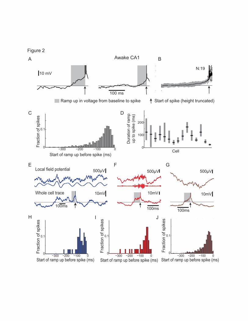
Ramp up in voltage from baseline to spike Start of spike (height truncated)

10 mVN:19

100 ms

A

C D

Start of ramp up before spike (ms)

Frac

tion

of s

pike

s

00

0.1

0

100

Dur

atio

n of

ram

pup

to s

pike

(ms)

Cell

Awake CA1

500μV

10mV

100ms

500μV

10mV

100ms

500μV

10mV

100ms

Whole cell trace

Local field potentialE

Frac

tion

of s

pike

s

00

0.1

Start of ramp up before spike (ms)

Frac

tion

of s

pike

s

00

0.1

Start of ramp up before spike (ms)

Frac

tion

of s

pike

s

00

0.1

B

F G

H I J

Start of ramp up before spike (ms)

Mean change frombaseline to threshold (mV)

5 10 15 20 25 30

Mea

n st

art o

f ram

p up

befo

re s

pike

(ms)

-160-140-120-100-80-60-40-20 r:-0.55

p<0.04

A

B

ff f ( )

-20 -10 0

Frac

tion

of ti

me

0

0.1

0.2

0.3

0.4

-200 -150 -100 -50 0

Cel

l

more unimodal

more bimodal

Mean baseline-70 -65 -60 -55 -50 -45

Mea

n st

art o

f ram

p up

befo

re s

pike

(ms)

-160

-140

-120

-100

-80

-60

-40

-20 r: 0.57p<0.03

Mean firing rate (Hz) 0 1 2 3 4

befo

re s

pike

(ms)

-160

-140

-120

-100

-80

-60

-40

-20 r: 0.59p<0.02

Figure 3

2010

Voltage difference from baseline (mV) Start of long ramp up before spike (ms)

membrane potential (mV)

Mea

n st

art o

f ram

p up

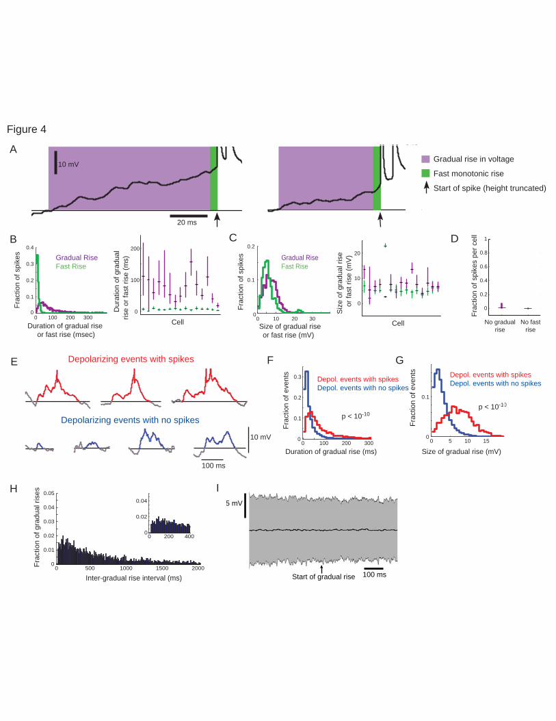
0

100

200

Cell

Dur

atio

n of

gra

dual

rise

or fa

st ri

se (m

s)

0

10

20

Cell

Siz

e of

gra

dual

rise

or

fast

rise

(mV

)

0 100 200 3000

0.1

0.2

0.3

0.4

Frac

tion

of s

pike

s

Duration of gradual rise or fast rise (msec)

0 10 20 300

0.1

0.2Fr

actio

n of

spi

kes

Size of gradual rise or fast rise (mV)

A

CB D

20 ms

10 mV

20 ms

Gradual rise in voltage

Fast monotonic rise

Start of spike (height truncated)

10 mV

100 ms

E F GDepolarizing events with spikes

Depolarizing events with no spikes

Gradual RiseFast Rise

Depol. events with spikesDepol. events with no spikes

p < 10-10p < 10-10

0 5 10 150

0.1

Frac

tion

of e

vent

s

Size of gradual rise (mV)0 100 200 300

0

0.1

0.2

0.3

Frac

tion

of e

vent

s

Duration of gradual rise (ms)

Gradual RiseFast Rise

Depol. events with spikesDepol. events with no spikes

0 500 1000 1500 20000

0.01

0.02

0.03

0.04

0.05

Inter-gradual rise interval (ms)

Frac

tion

of g

radu

al ri

ses

0 200 4000

0.02

0.04 5 mV

100 msStart of gradual rise

H I

Figure 4

0

0.2

0.4

0.6

0.8

1

No gradualrise

No fastrise

Frac

tion

of s

pike

s pe

r cel

l

CA1 in awake miceCA B

0

50

100

CellD

urat

ion

of g

radu

al

or f

ast r

ise

(ms)

0

50

100

Cell

Dur

atio

n of

ram

pup

to s

pike

(ms)

00

0.1

Start of ramp up before spike (ms)

Frac

tion

of s

pike

s

Figure 5

A Monotonically increasing events

Change in voltage during fast rise (mV)

Dur

atio

n fa

st in

crea

se

in v

olta

ge (m

s)

Prob

abilit

y of

spi

king

20

10

00 5 10

1

0.8

0.6

0.4

0.2

0

20 mV

100 ms

B

Figure 6

Gradual rise

No gradual rise

Pro

babi

lity

of s

piki

ngin

resp

onse

to p

ulse

(%)

0

20

40

60

80

1001.5-3.7% 12-27% 37-61%

Pro

babi

lity

of s

piki

ngin

resp

onse

to p

ulse

(%)

1.5-3.7%, 1-2mV 12-27%, 1-2mV 37-61%, 1-2mV 1.5-3.7%, 2-5mV 12-27%, 2-5mV 1.5-3.7%, 5-7mV 37-61%, 5-7mV

0

20

40

60

80

100

0-10 ms ramp-up

50-200 ms ramp-up

CCell’s overall spike probability

Overall spike probability, size ramp-up

A

B

Start of ramp up before spike (ms)

Frac

tion

of s

pike

s

C

Awake Barrel Cortex

Ramp up in voltage from baseline to spike Start of spike (height truncated)

Dur

atio

n of

Ram

pU

p to

Spi

ke (m

s)

Cell

D

Figure 7

Frac

tion

of s

pike

s

Duration of gradual rise or fast rise (ms)

Frac

tion

of s

pike

s

Stize of gradual rise

Monotonically increasing events

Change in voltage during fast rise (m )

Dur

atio

n fa

st in

crea

se

in v

olta

ge (m

s)

Prob

abili

ty o

f spi

king

G H IDepolarizing events with spikes

Depolarizing events with no spikes

Frac

tion

of e

vent

s

Duration of gradual rise (ms)5

Frac

tion

of e

vent

s

E F

J K

Cell

Size

of g

radu

al ri

se

Cell

Dur

atio

n of

gra

dual

Inter-gradual Rise Interval (ms)

Frac

tion

of G

radu

al R

ises

No gradualrise

No fastrise

Frac

tion

of s

pike

s pe

r cel

l

A

0 1 2 3

0

Mean firing rate (Hz)

Mea

n st

art o

f ram

p up

be

fore

spi

kes

(mse

c)0

Mean baseline membrane potential (mV)

Mea

n st

art o

f ram

p up

be

fore

spi

kes

(mse

c)

0 10 20 30

0

Mean change from baseline to threshold (mV)

Mea

n st

art o

f ram

p up

be

fore

spi

kes

(ms)

n.s.n.s.n.s.

0 10 20 300

0.1

0.2

0.3

Frac

tion

of ti

me

Voltage difference from baseline (mV)0 10 20 300

0.1

Frac

tion

of ti

me

0 10 20 300

0.1

0.2

0

Start of long ramp up before spike (ms)

Cel

l

more unimodal

more bimodal

B

Voltage difference from baseline (mV)Voltage difference from baseline (mV)

Frac

tion

of ti

me

BA

DC

0

0.1

0.2

0.3

0.4

0.5

0.6

0.7

50 100 150 200 250

4mV

8mV

12mV

Duration of gradual rise (ms)

Spi

ke p

roba

bilit

y

0

0.1

0.2

0.3

0.4

0.5

0.6

0.7

50 100 150 200 2504mV

12mV

20mV

Duration of gradual rise (ms)

Spi

ke p

roba

bilit

y

50 100 150 200 2500

0.2

0.4

0.6

0.8

1

Duration of gradual rise (ms)

Spi

ke p

roba

bilit

y

50 100 150 200 2500

0.2

0.4

0.6

0.8

1

Duration of gradual rise (ms)

Spi

ke p

roba

bilit

y

Cha

nge

in v

olta

ge

durin

g fa

st ri

se (m

V)

D

urat

ion

of fa

stris

e in

vol

tage

(ms)

Duration of gradual rise in voltage (ms)

Pro

babi

lity

of s

piki

ngP

roba

bilit

y of

spi

king

Change in voltage duringgradual rise (mV)

Hippocampal CA1 in awake mice

Barrel cortex in awake mice

Depolarizing events

Depolarizing events

Figure 9

Cha

nge

in v

olta

ge

durin

g fa

st ri

se (m

V)

Dur

atio

n of

fast

rise

in v

olta

ge (m

s)

Duration of gradual rise in voltage (ms)

Change in voltage duringgradual rise (mV)

Prob

abilit

y of

spi

king

Prob

abilit

y of

spi

king

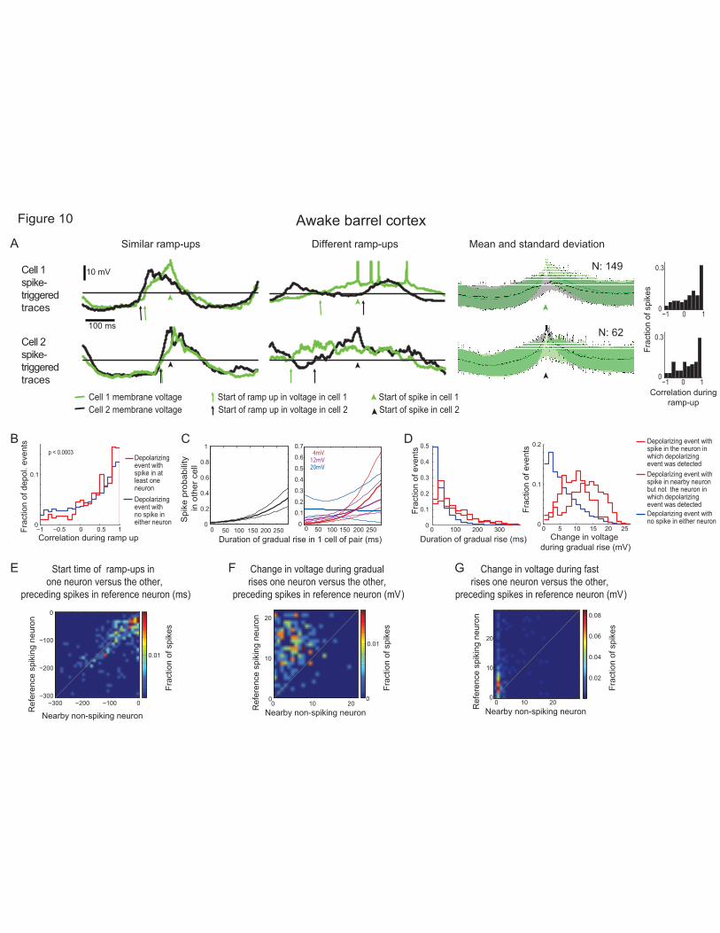
A

N: 149

B C D

E

N: 62

0 10

0.3

0 10

0.3

Similar ramp-ups Mean and standard deviation

Cell 1 spike-triggeredtraces

Cell 1 membrane voltage Start of ramp up in voltage in cell 1 Start of spike in cell 1Cell 2 membrane voltage Start of ramp up in voltage in cell 2 Start of spike in cell 2

Awake barrel cortex

F

0 10 200

10

20

0

0.01

Nearby non-spiking neuronRef

eren

ce s

piki

ng n

euro

n

0 10 200

10

20

0.02

0.04

0.06

0.08

Nearby non-spiking neuronRef

eren

ce s

piki

ng n

euro

n

Start time of ramp-ups in one neuron versus the other,

preceding spikes in reference neuron (ms)

Change in voltage during gradual rises one neuron versus the other,

preceding spikes in reference neuron (mV)

Change in voltage during fast rises one neuron versus the other,

preceding spikes in reference neuron (mV)

G

Duration of gradual rise in 1 cell of pair (ms)

Spi

ke p

roba

bilit

y in

oth

er c

ell

Depolarizing event with spike in the neuron in which depolarizing event was detectedDepolarizing event with spike in nearby neuron but not the neuron in which depolarizing event was detectedDepolarizing event with no spike in either neuron

0 100 200 3000

0.1

0.2

0.3

0.4

0.5

Frac

tion

of e

vent

s

Duration of gradual rise (ms)

0 5 10 15 20 250

0.1

0.2

Frac

tion

of e

vent

sChange in voltage

during gradual rise (mV)

0 0.5 10

0.1

Correlation during ramp up

Frac

tion

of d

epol

. eve

nts

p < 0.0003Depolarizing event with spike in at least one neuron Depolarizing event with no spike in either neuron 0

0.2

0.4

0.6

0.8

1

0

0.1

0.2

0.3

0.4

0.5

0.6

0.7

50 100 150 200 250

4mV12mV20mV

0

0

0.01

Nearby non-spiking neuron

Ref

eren

ce s

piki

ng n

euro

n

Frac

tion

of s

pike

s

Frac

tion

of s

pike

s

Different ramp-ups

10 mV

100 ms

Frac

tion

of s

pike

s

Correlation duringramp-up

Figure 10

Cell 2 spike-triggeredtraces

00 50 100 150 200 250

Frac

tion

of s

pike

s

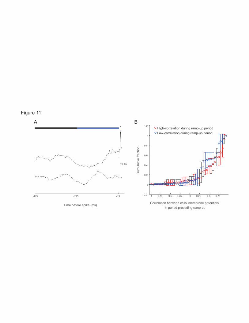
Correlation between cells’ membrane potentialsin period preceding ramp-up

-0.75 -0.5 -0.25 0 0.25 0.5 0.75

High-correlation during ramp-up periodLow-correlation during ramp-up period

-1

Cum

ulat

ive

fract

ion

-0.2

0

0.2

0.4

0.6

0.8

1

1.2B

*A

-415 -215 -15

Time before spike (ms)

10 mV

Figure 11