Meso-NH model

40 users laboratories

A research model, jointly developped by Meteo-France and Laboratoire d’Aérologie (CNRS/UPS)

http://mesonh.aero.obs-mip.fr/mesonh/

Plan

1. General presentation of the model

2. Meso-scale simulations.

3. Large-Eddy simulations

4. Atmospheric Chemistry

5. New couplings : Electricity, Hydrology, Dispersion

6. Climatology

7. Diagnostics

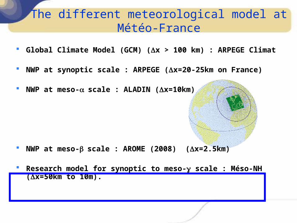
The different meteorological model at Météo-France

Global Climate Model (GCM) (x > 100 km) : ARPEGE Climat

NWP at synoptic scale : ARPEGE (x=20-25km on France)

NWP at meso-scale : ALADIN (x=10km)

NWP at meso-scale : AROME (2008) (x=2.5km)

Research model for synoptic to meso- scale : Méso-NH (x=50km to 10m).

Why do we need a high resolution research model ?

1. To improve parameterizations for Large Scale models : fine resolution simulations allow to resolve the main coherent patterns and inform on fine scale

variability.

2. To help the evaluation and the improvement of AROME

3. To better understand the physics (e.g. cloud processes), to characterize local effects

4. To carry out impact studies and use the model as a laboratory

5. To develop new couplings (e.g. Electricity, Hydrology …)

A broad variety of developments and applications

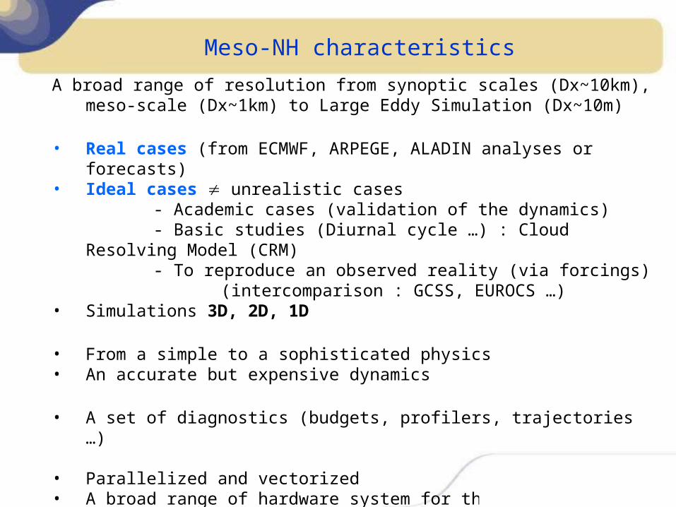
A broad range of resolution from synoptic scales (Dx~10km), meso-scale (Dx~1km) to Large Eddy Simulation (Dx~10m)

• Real cases (from ECMWF, ARPEGE, ALADIN analyses or forecasts)• Ideal cases unrealistic cases

- Academic cases (validation of the dynamics)- Basic studies (Diurnal cycle …) : Cloud Resolving Model (CRM)- To reproduce an observed reality (via forcings)

(intercomparison : GCSS, EUROCS …)• Simulations 3D, 2D, 1D

• From a simple to a sophisticated physics• An accurate but expensive dynamics

• A set of diagnostics (budgets, profilers, trajectories …)

• Parallelized and vectorized• A broad range of hardware system for the research community : FUJITSU,

NEC, CRAY, IBM, cluster of PC

No operational objective.

Meso-NH characteristics

The meso-scale simulations with Meso-NH : 1km<x<10km

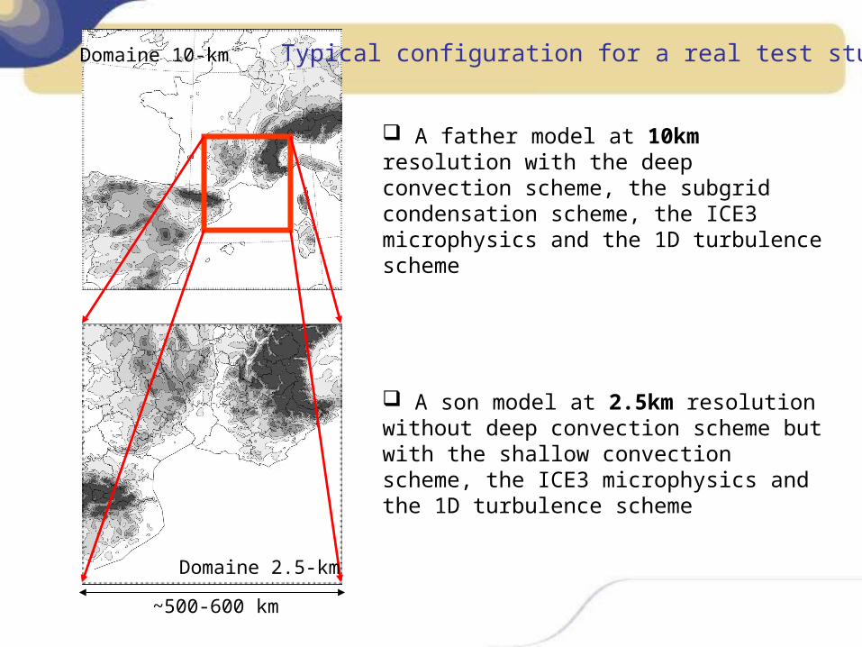
Domaine 10-km

~500-600 km

Domaine 2.5-km

Typical configuration for a real test study

A father model at 10km resolution with the deep convection scheme, the subgrid condensation scheme, the ICE3 microphysics and the 1D turbulence scheme

A son model at 2.5km resolution without deep convection scheme but with the shallow convection scheme, the ICE3 microphysics and the 1D turbulence scheme

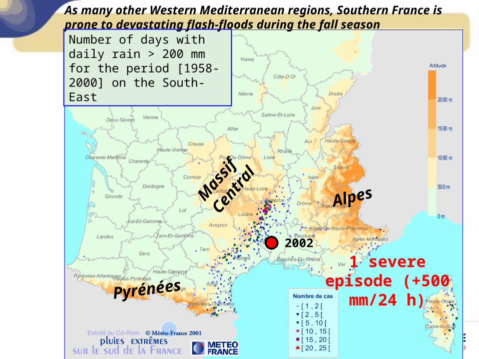
Number of days with daily rain > 200 mm for the period [1958-2000] on the South-East

Mas

sif

Cent

ral

Alpes

Pyrénées

1 severe episode (+500

mm/24 h)

2002

As many other Western Mediterranean regions, Southern France is prone to devastating flash-floods during the fall season

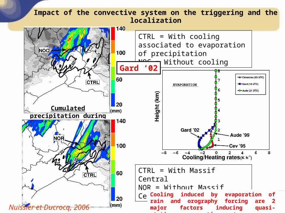
Impact of the convective system on the triggering and the localization

CTRL = With cooling associated to evaporation of precipitationNOC = Without cooling

Cumulated precipitation during

4 hours

Gard ‘02

CTRL = With Massif CentralNOR = Without Massif Central

Nuissier et Ducrocq, 2006

Cooling induced by evaporation of rain and orography forcing are 2 major factors inducing quasi-stationary convective systems

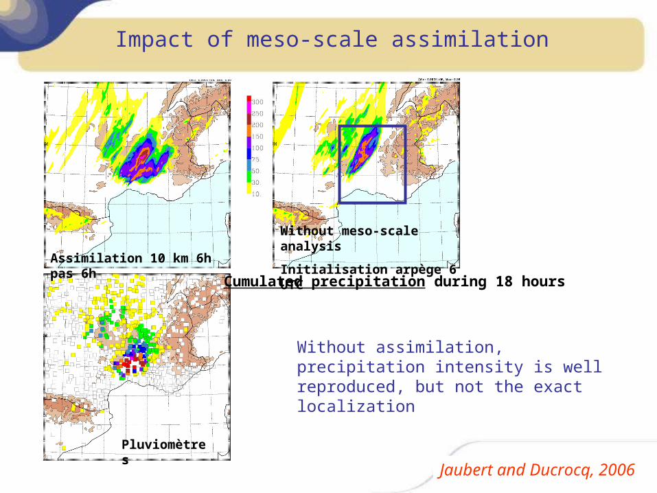
Pluviomètres

Assimilation 10 km 6h pas 6h

Without meso-scale analysis

Initialisation arpège 6 UTC

Without assimilation, precipitation intensity is well reproduced, but not the exact localization

Jaubert and Ducrocq, 2006

Cumulated precipitation during 18 hours

Impact of meso-scale assimilation

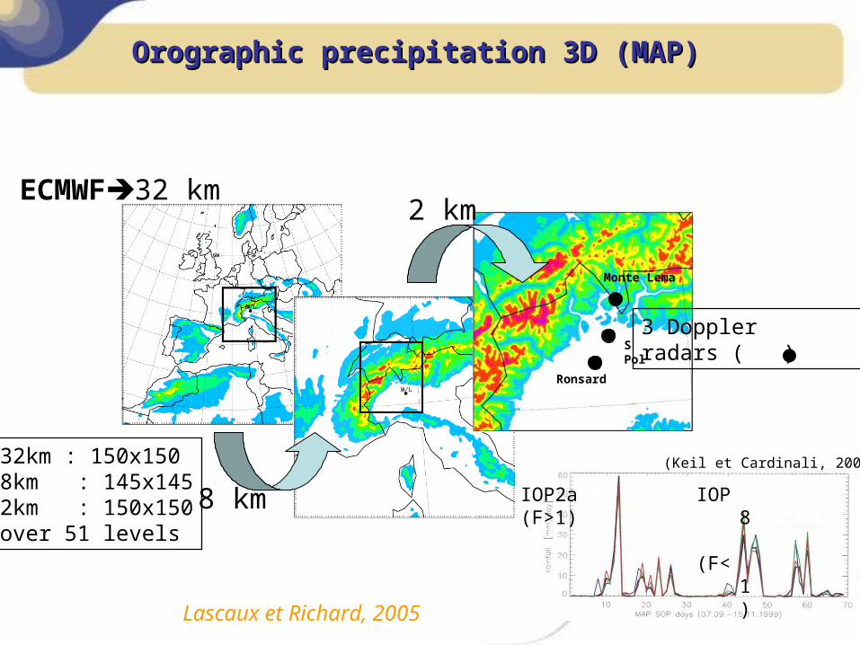
(Keil et Cardinali, 2003)32km : 150x1508km : 145x1452km : 150x150over 51 levels

IOP8 (F<1)

IOP2a(F>1)

8 km

2 km

Monte Lema

S Pol

Ronsard

ECMWF32 km

3 Dopplerradars ( )

Orographic precipitation 3D (MAP)Orographic precipitation 3D (MAP)

How can dynamics modify the microphysics ?

Lascaux et Richard, 2005

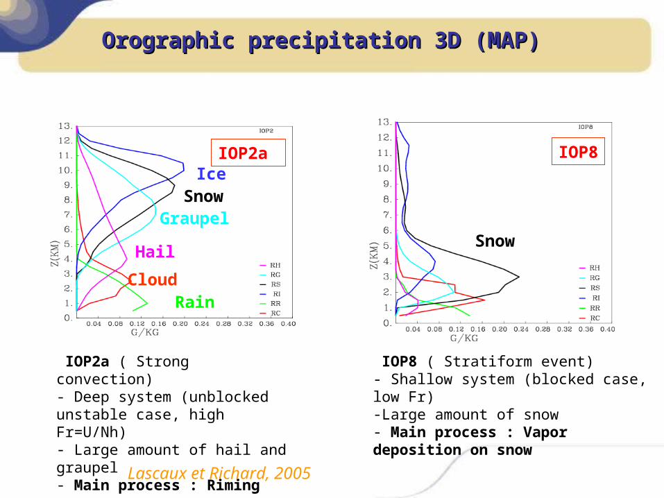
SnowGraupel

Hail

Cloud Rain

IceIOP2a

IOP2a ( Strong convection)- Deep system (unblocked unstable case, high Fr=U/Nh)- Large amount of hail and graupel- Main process : Riming

Mean vertical distribution of hydrometeors

IOP8 ( Stratiform event)- Shallow system (blocked case, low Fr)-Large amount of snow- Main process : Vapor deposition on snow

IOP8

Snow

Lascaux et Richard, 2005

Orographic precipitation 3D (MAP)Orographic precipitation 3D (MAP)

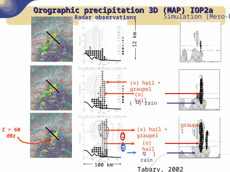
Z > 60 dBz

12

km

100 kmTabary, 2002

(x) hail + graupel

(o) hail

( ) rain

(o) hail

(x) hail + graupel

( ) rain

graupel

Simulation (Meso-NH)Orographic precipitation 3D (MAP) IOP2aOrographic precipitation 3D (MAP) IOP2a

Radar observations

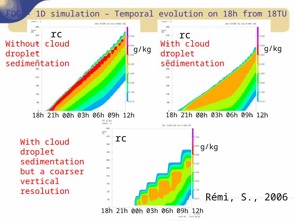
FOG – 1D simulation – Temporal evolution on 18h from 18TU

rc rc

rc

Without cloud droplet sedimentation

With cloud droplet sedimentation

With cloud droplet sedimentation but a coarser vertical resolution

Rémi, S., 2006

18h 21h 00h 03h 06h 09h 12h 18h 21h 00h 03h 06h 09h 12h

18h 21h 00h 03h 06h 09h 12h

g/kg g/kg

g/kg

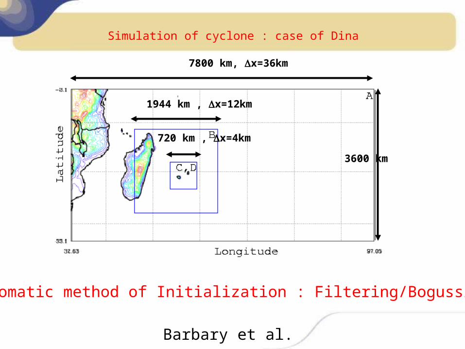
Simulation of cyclone : case of Dina

7800 km, x=36km

1944 km , x=12km

720 km , x=4km

3600 km

Automatic method of Initialization : Filtering/Bogussing

Barbary et al.

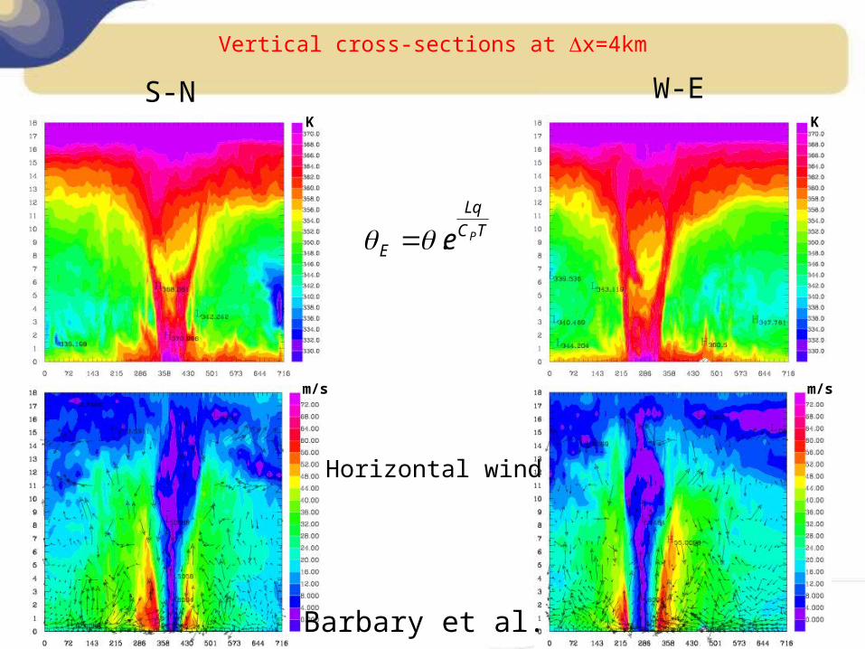
Vertical cross-sections at x=4km

K

m/s

K

m/s

TC

Lq

EPe.

Horizontal wind

S-N W-E

Barbary et al.

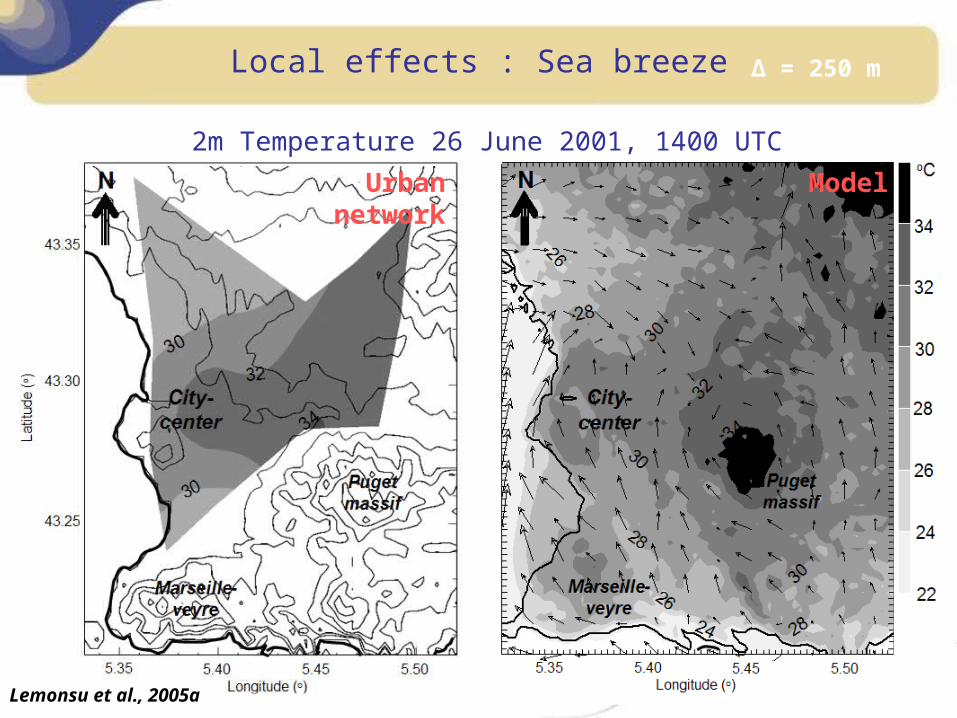
Local effects : Sea breeze

Urban network

Model

Lemonsu et al., 2005a

2m Temperature 26 June 2001, 1400 UTC

Δ = 250 m

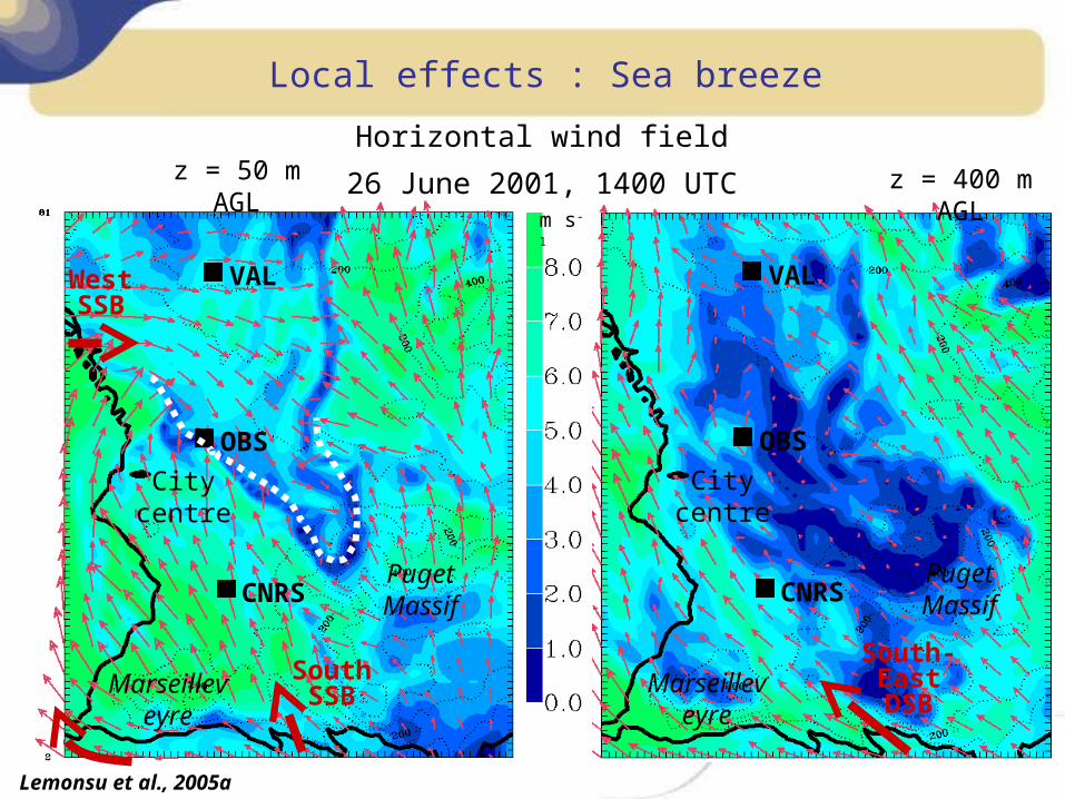
VAL

OBS

CNRSPuget Massif

Marseilleveyre

City centre

z = 400 m AGL

VAL

OBS

CNRS

m s-1

Puget Massif

Marseilleveyre

City centre

z = 50 m AGL

West SSB

South SSB

South-East DSB

Horizontal wind field

26 June 2001, 1400 UTC

Lemonsu et al., 2005a

Local effects : Sea breeze

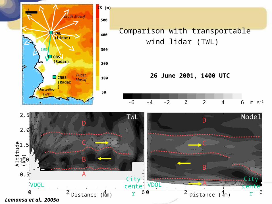
6 m s-1420-2-4-6

26 June 2001, 1400 UTC

B

C

D

A

TWL

B

C

D

A

Model

VDOLCity

center0 2 4 6 0 2 4 6Distance (km) Distance (km)

VDOLCity

center

0.5

1.0

1.5

2.0

2.5

Alt

itude (

km

)500

400

300

200

100

50

ZS (m)

Marseilleveyre

190o

Puget MassifCNRS

(Radar)

3 km

VAL (Lidar)

OBS (Radar)

Etoile Massif

Comparison with transportable wind lidar (TWL)

Lemonsu et al., 2005a

The Large Eddy Simulations with Meso-NH :

Large eddys are resolved : TKEresolved >> TKE Subgrid

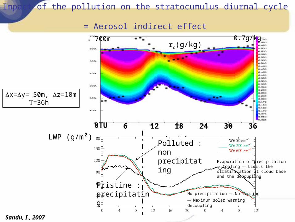
Impact of the pollution on the stratocumulus diurnal cycle = Aerosol indirect effect

0.7g/kg700mrc(g/kg)

Simulation LES 50mNuage non pollué

Sandu, I., 2007

0TU 6 12 18 24 30 36

x=y= 50m, z=10m=36h

LWP (g/m²)Polluted : non precipitating

Pristine : precipitating

Evaporation of precipitation Cooling Limits the stratification at cloud base and the decoupling

No precipitation No Cooling

Maximum solar warming decoupling

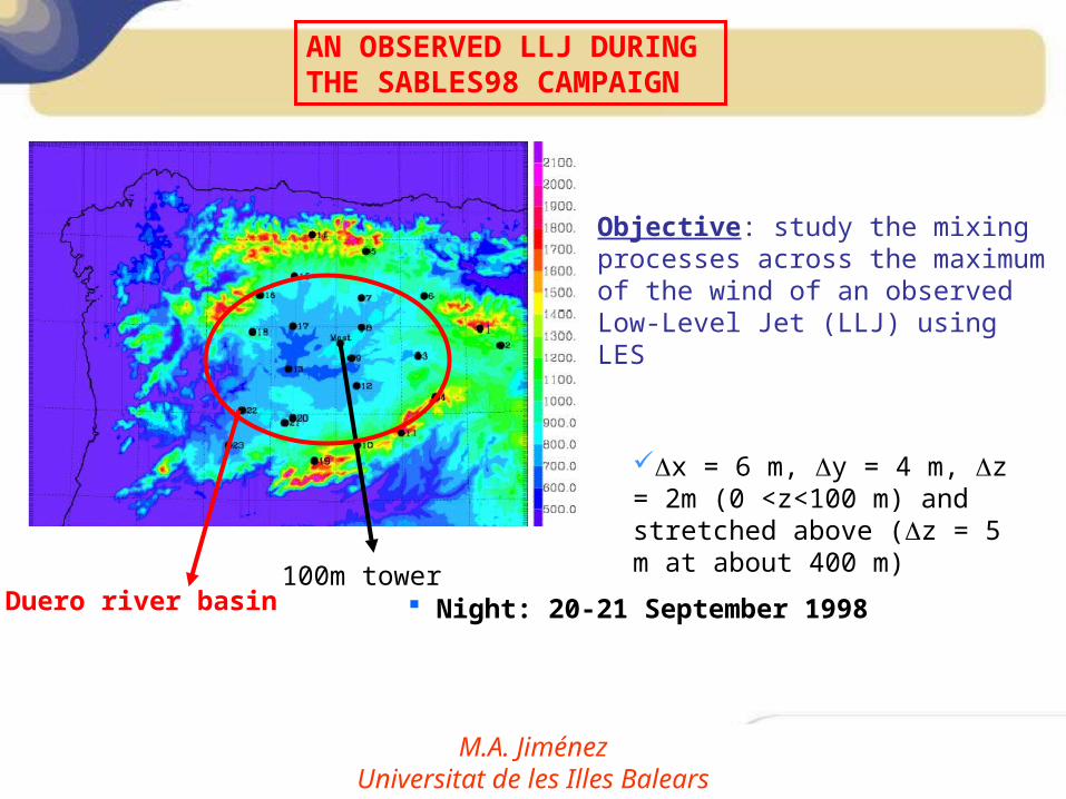
AN OBSERVED LLJ DURING THE SABLES98 CAMPAIGN

Night: 20-21 September 1998100m tower

Duero river basin

x = 6 m, y = 4 m, z = 2m (0 <z<100 m) and stretched above (z = 5 m at about 400 m)

M.A. JiménezUniversitat de les Illes Balears

Objective: study the mixing processes across the maximum of the wind of an observed Low-Level Jet (LLJ) using LES

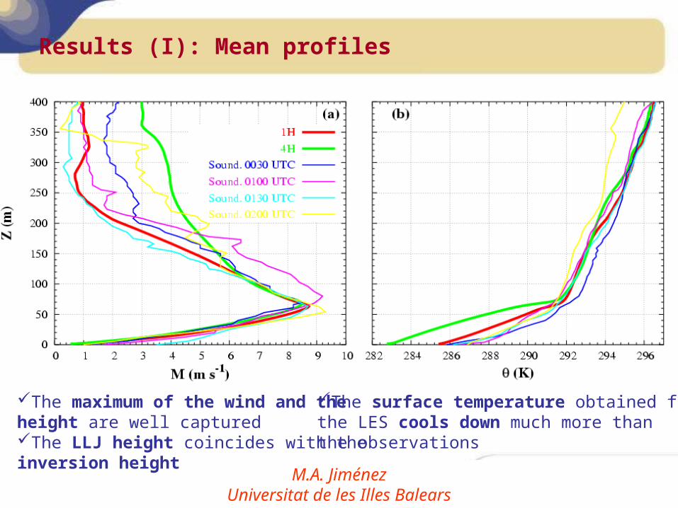
Results (I): Mean profiles

M.A. JiménezUniversitat de les Illes Balears

The maximum of the wind and the height are well capturedThe LLJ height coincides with theinversion height

The surface temperature obtained fromthe LES cools down much more thanthe observations

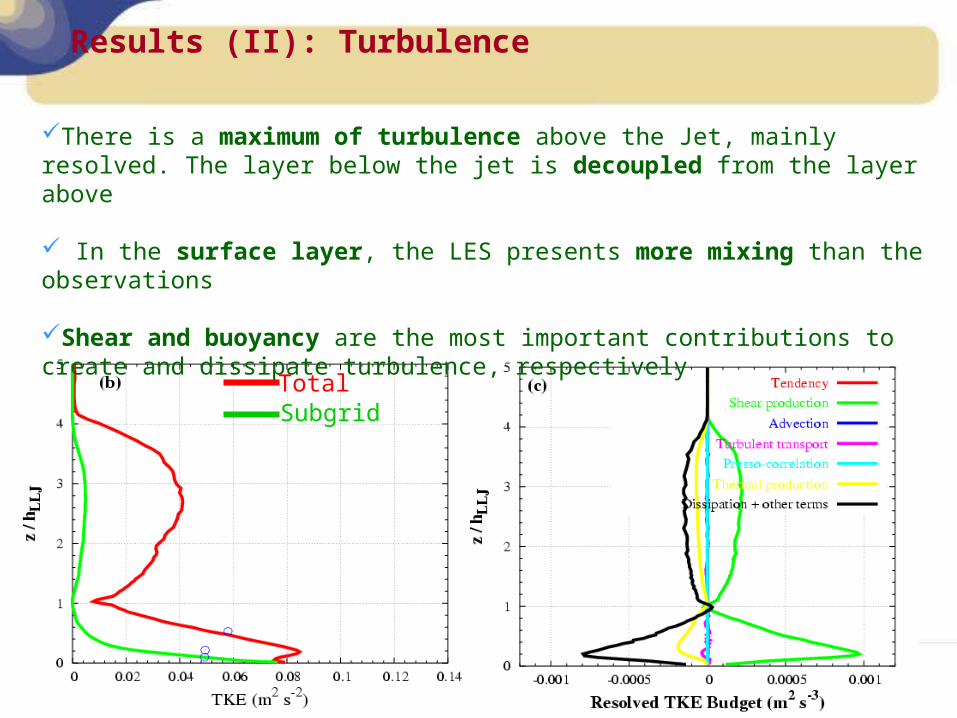
Results (II): Turbulence

There is a maximum of turbulence above the Jet, mainly resolved. The layer below the jet is decoupled from the layer above

In the surface layer, the LES presents more mixing than the observations

Shear and buoyancy are the most important contributions to create and dissipate turbulence, respectively

TotalSubgrid

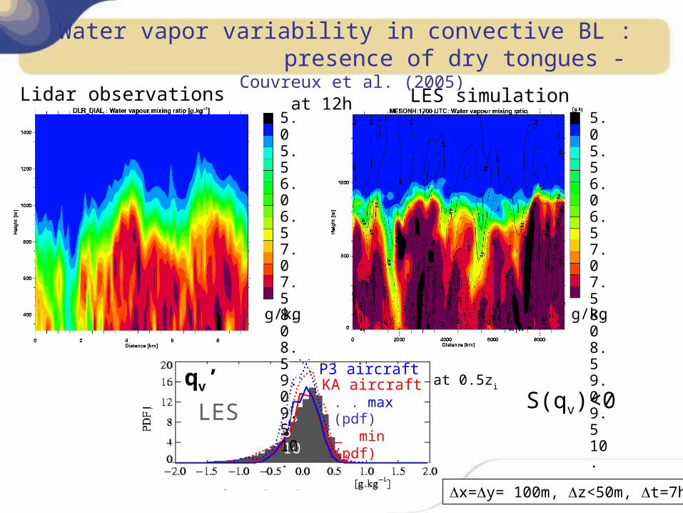
Lidar observationsLES Simulations

rv’

LES simulation5.05.56.06.57.07.58.08.59.09.510.

5.05.56.06.57.07.58.08.59.09.510.

5.05.56.06.57.07.58.08.59.09.510.

5.05.56.06.57.07.58.08.59.09.510.

g/kg g/kg

P3 aircraftKA aircraft. . max (pdf)_ min (pdf)LES

qv’ at 0.5zi

Water vapor variability in convective BL : presence of dry tongues - Couvreux et al. (2005)

at 12h

x=y= 100m, z<50m, t=7h

S(qv)<0

Atmospheric Chemistry

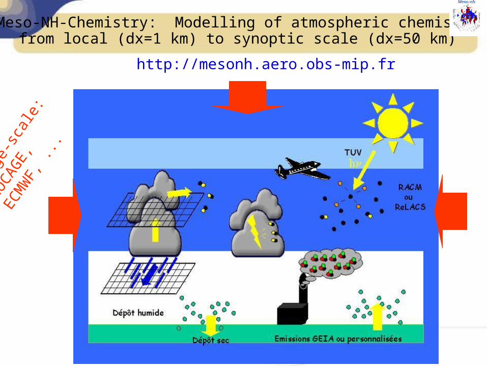
Meso-NH-Chemistry: Modelling of atmospheric chemistry from local (dx=1 km) to synoptic scale (dx=50 km)

http://mesonh.aero.obs-mip.fr

larg

e-sc

ale:

MO

CAGE,

ECM

WF,

...

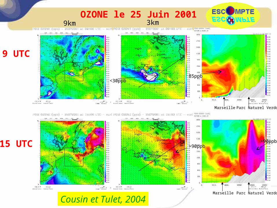
OZONE le 25 Juin 2001

9 UTC

9km 3km

<30ppb

Parc Naturel VerdonMarseille

85ppb

Marseille Parc Naturel Verdon

>90ppb15 UTC >90ppb

Cousin et Tulet, 2004

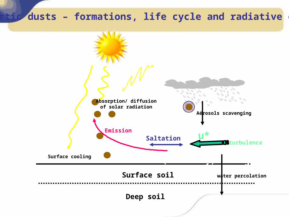
surfacewater percolation

Deep soil

Surface soil

Soil (sand/clay)

Aérosols scavenging

Absorption/ diffusionof solar radiation

Surface cooling

Desertic dusts – formations, life cycle and radiative effect

u*turbulence

Emission

Saltation

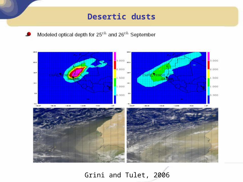
Desertic dusts

Grini and Tulet, 2006

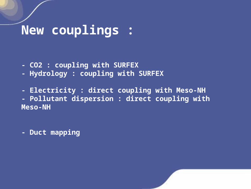
New couplings :

- CO2 : coupling with SURFEX - Hydrology : coupling with SURFEX

- Electricity : direct coupling with Meso-NH- Pollutant dispersion : direct coupling with Meso-NH

- Duct mapping

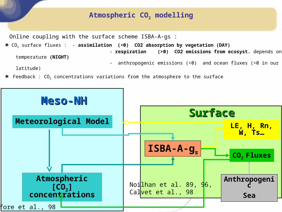
Atmospheric CO2 modelling

Online coupling with the surface scheme ISBA-A-gs :

CO2 surface fluxes : - assimilation (<0) CO2 absorption by vegetation (DAY) - respiration (>0) CO2 emissions from ecosyst. depends on temperature (NIGHT) - anthropogenic emissions (>0) and ocean fluxes (<0 in our latitude)

Feedback : CO2 concentrations variations from the atmosphere to the surface

ISBA-A-gs

Meteorological Model LE, H, Rn, W, Ts…

Atmospheric [CO2]

concentrations

Anthropogenic

Sea

Meso-NHMeso-NHSurfaceSurface

Lafore et al., 98

Noilhan et al. 89, 96, Calvet et al., 98

CO2 Fluxes

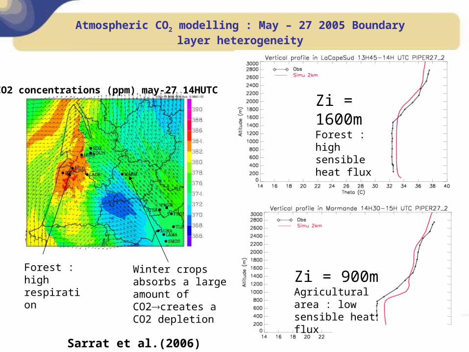
Sarrat et al.(2006)

CO2 concentrations (ppm) may-27 14HUTC

Atmospheric CO2 modelling : May – 27 2005 Boundary layer heterogeneity

Winter crops absorbs a large amount of CO2creates a CO2 depletion

Zi = 900mAgricultural area : low sensible heat flux

Zi = 1600mForest : high sensible heat flux

Forest : high respiration

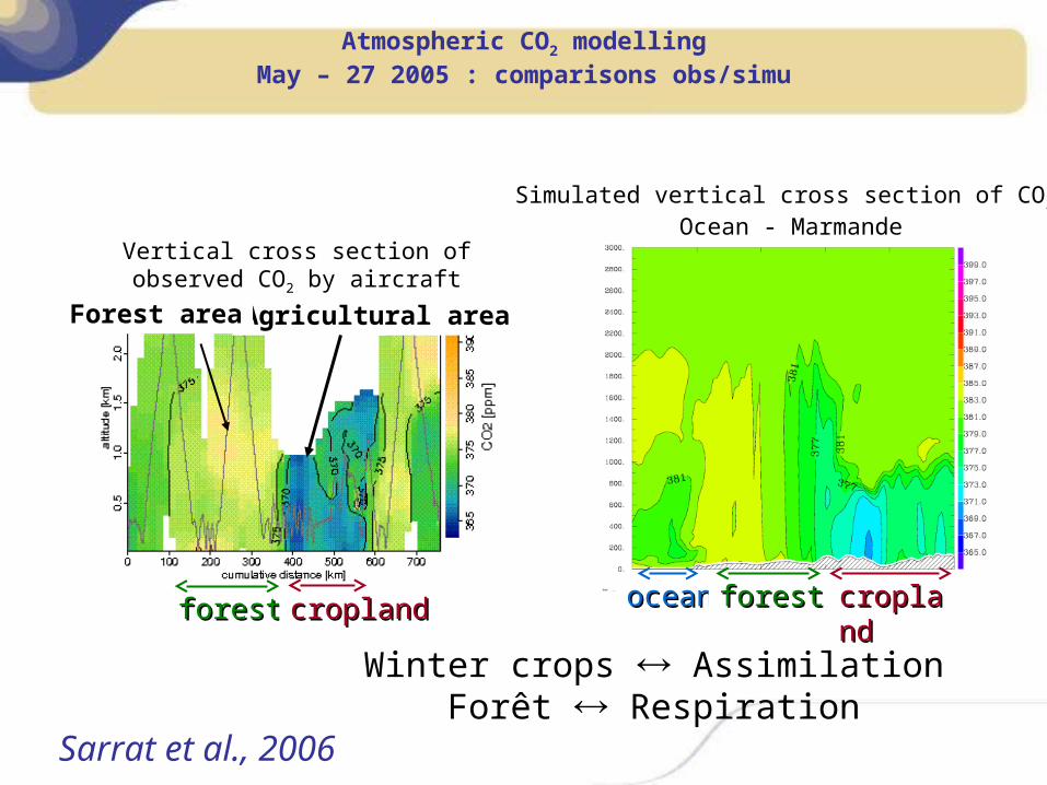
Atmospheric CO2 modellingMay – 27 2005 : comparisons obs/simu

Simulated vertical cross section of CO2 Ocean - Marmande

Agricultural areaForest area

Vertical cross section of observed CO2 by aircraft

oceanocean forestforest croplandcroplandforestforest croplandcropland

Sarrat et al., 2006

Winter crops AssimilationForêt Respiration

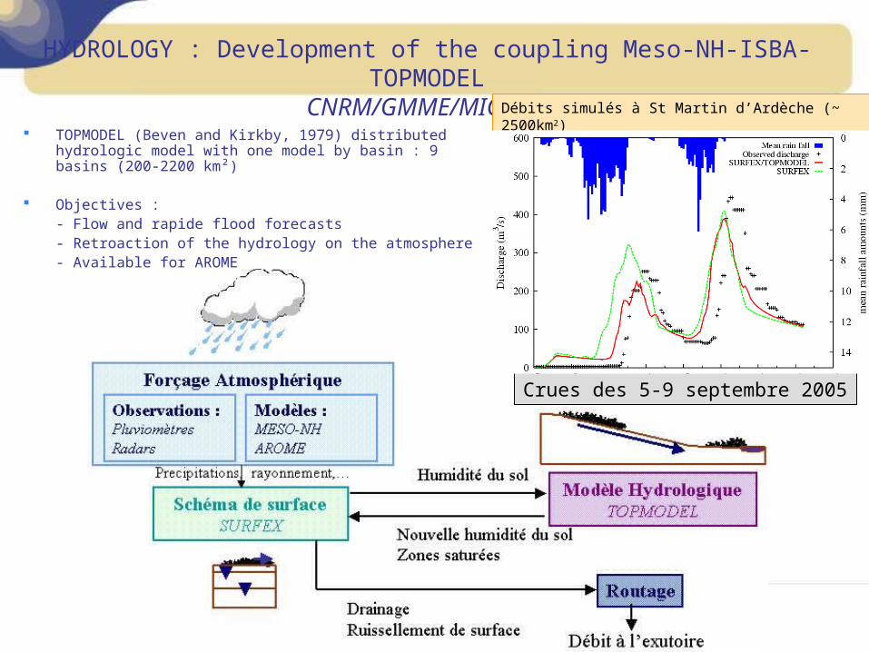
TOPMODEL (Beven and Kirkby, 1979) distributed hydrologic model with one model by basin : 9 basins (200-2200 km²)

Objectives :- Flow and rapide flood forecasts- Retroaction of the hydrology on the atmosphere- Available for AROME

HYDROLOGY : Development of the coupling Meso-NH-ISBA-TOPMODELCNRM/GMME/MICADO

Crues des 5-9 septembre 2005

Débits simulés à St Martin d’Ardèche (~ 2500km2)

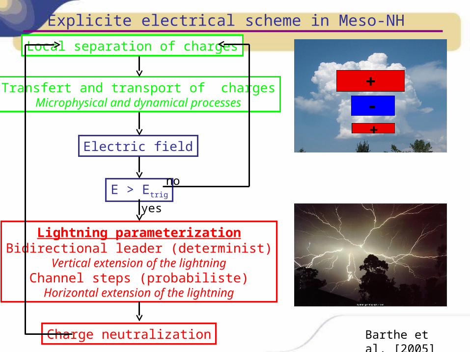
Barthe et al. [2005]

+

+

-

Explicite electrical scheme in Meso-NH

Local separation of charges

Transfert and transport of chargesMicrophysical and dynamical processes

Electric field

Lightning parameterizationBidirectional leader (determinist)

Vertical extension of the lightningChannel steps (probabiliste)

Horizontal extension of the lightning

Charge neutralization

E > Etrig

yes

no

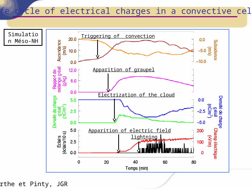
Life cycle of electrical charges in a convective cell

Barthe et Pinty, JGR

Apparition of graupel

Electrization of the cloud

Apparition of electric fieldlightning

Triggering of convectionSimulation Méso-NH

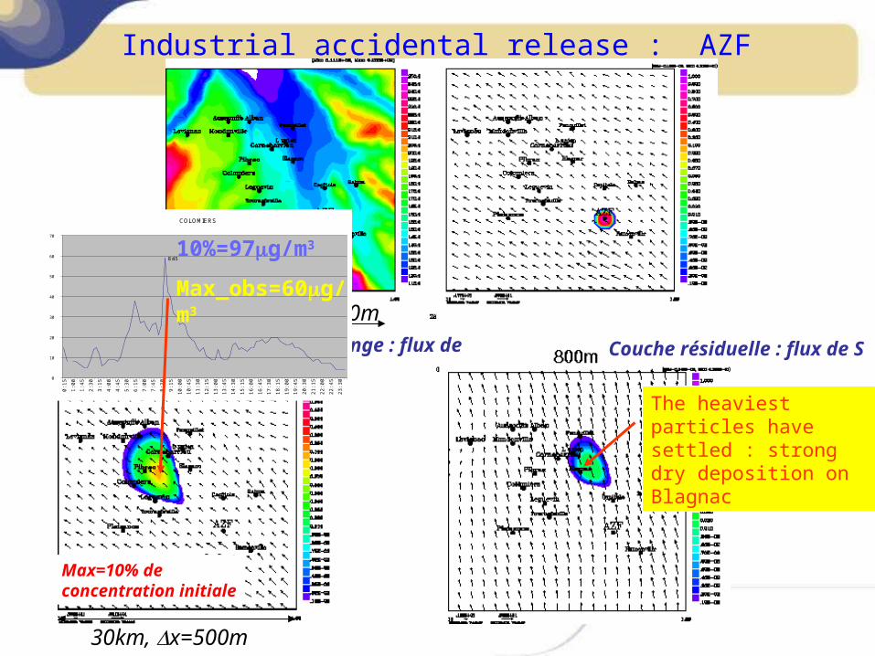
30km, x=500m

Industrial accidental release : AZF

Couche résiduelle : flux de SCouche de mélange : flux de SE

Max=10% de concentration initiale

30km, x=500m

COLOMIERS

8:45

0

10

20

30

40

50

60

70

0:1

5

1:0

0

1:4

5

2:3

0

3:1

5

4:0

0

4:4

5

5:3

0

6:1

5

7:0

0

7:4

5

8:3

0

9:1

5

10

:00

10

:45

11:3

0

12

:15

13

:00

13

:45

14

:30

15

:15

16

:00

16

:45

17

:30

18

:15

19

:00

19

:45

20

:30

21

:15

22

:00

22

:45

23

:30

10%=97g/m3

Max_obs=60g/m3

The heaviest particles have settled : strong dry deposition on Blagnac

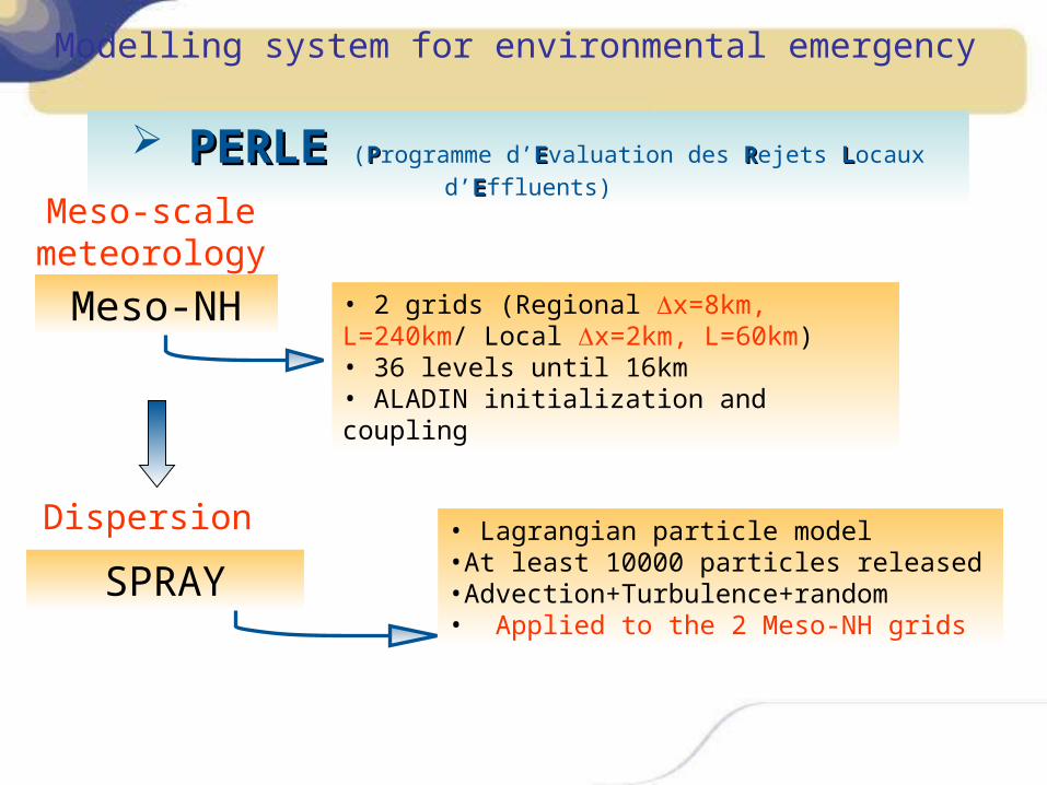
SPRAY• Lagrangian particle model•At least 10000 particles released •Advection+Turbulence+random• Applied to the 2 Meso-NH grids

PERLEPERLE (PProgramme d’EEvaluation des RRejets L Locaux d’EEffluents)

Dispersion

Meso-NH • 2 grids (Regional x=8km, L=240km/ Local x=2km, L=60km)• 36 levels until 16km• ALADIN initialization and coupling

Meso-scale meteorology

Modelling system for environmental emergency

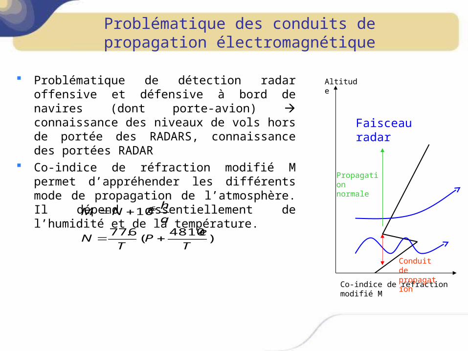
Problématique des conduits de propagation électromagnétique

Problématique de détection radar offensive et défensive à bord de navires (dont porte-avion) connaissance des niveaux de vols hors de portée des RADARS, connaissance des portées RADAR

Co-indice de réfraction modifié M permet d’appréhender les différents mode de propagation de l’atmosphère. Il dépend essentiellement de l’humidité et de la température.

Co-indice de réfraction modifié M

Altitude

Conduit de propagation

Faisceau radar

Propagation normale

)4810

(6.77

106

T

eP

TN

a

hNM

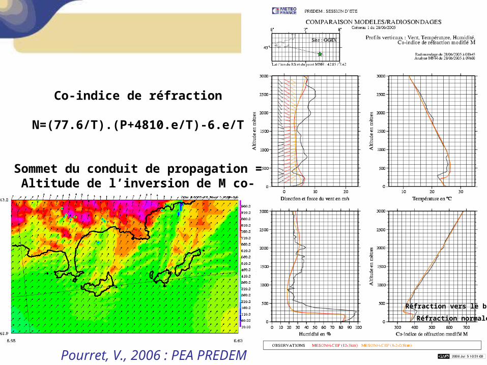
Pourret, V., 2006 : PEA PREDEM

Co-indice de réfraction

N=(77.6/T).(P+4810.e/T)-6.e/T

Sommet du conduit de propagation = Altitude de l’inversion de M co-indice de réfraction

OG dans le sillage des îles au sommet du conduit

Réfraction normale

Réfraction vers le bas

Climatologie . Régionalisation climatique

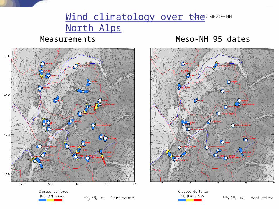
Roses Aladin 3 ansMéso-NH 95 dates Measurements

Wind climatology over the North Alps

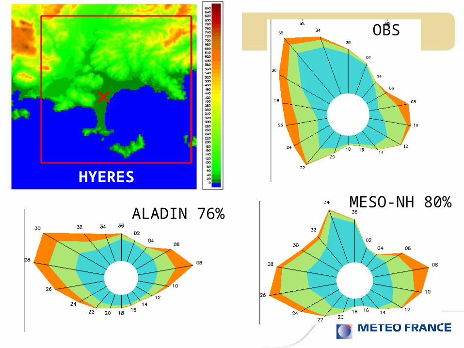
OBS

ALADIN 76%MESO-NH 80%

HYERES

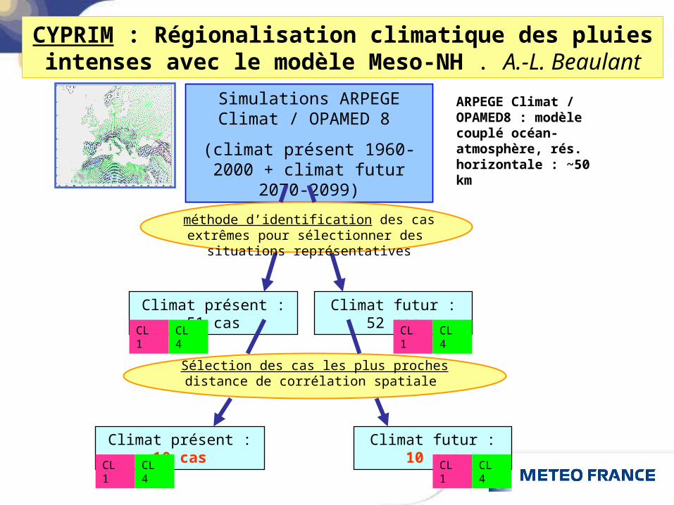
Climat futur : 52 cas

ARPEGE Climat / OPAMED8 : modèle couplé océan-atmosphère, rés. horizontale : ~50 km

Simulations ARPEGE Climat / OPAMED 8

(climat présent 1960-2000 + climat futur 2070-2099)

Climat présent : 51 cas

méthode d’identification des cas extrêmes pour sélectionner des situations

représentatives

CL 1 CL 4 CL 1 CL 4

Sélection des cas les plus prochesdistance de corrélation spatiale

Climat futur : 10 casClimat présent : 10 cas

CL 1 CL 4 CL 1 CL 4

CYPRIM : Régionalisation climatique des pluies intenses avec le modèle Meso-NH . A.-L. Beaulant

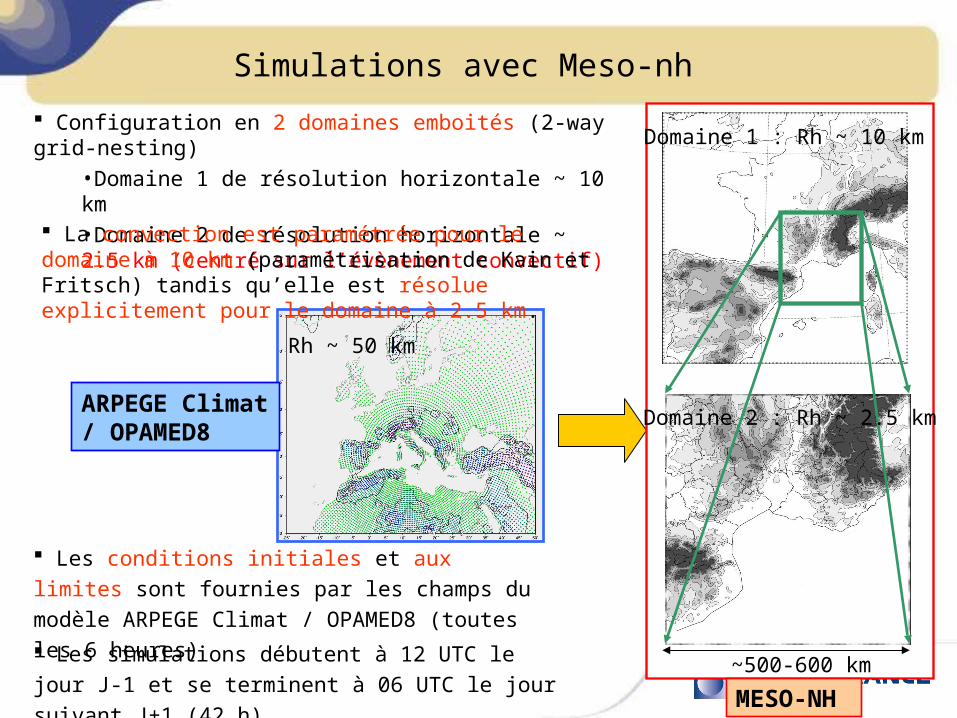
Simulations avec Meso-nh

Configuration en 2 domaines emboités (2-way grid-nesting)

•Domaine 1 de résolution horizontale ~ 10 km•Domaine 2 de résolution horizontale ~ 2.5 km (centré sur l’évènement convectif)

Les simulations débutent à 12 UTC le jour J-1 et se terminent à 06 UTC le jour suivant J+1 (42 h)

ARPEGE Climat / OPAMED8

~500-600 km

Domaine 1 : Rh ~ 10 km

Domaine 2 : Rh ~ 2.5 km

MESO-NH

Les conditions initiales et aux limites sont fournies par les champs du modèle ARPEGE Climat / OPAMED8 (toutes les 6 heures)

Rh ~ 50 km

La convection est paramétrée pour le domaine à 10 km (paramétrisation de Kain et Fritsch) tandis qu’elle est résolue explicitement pour le domaine à 2.5 km.

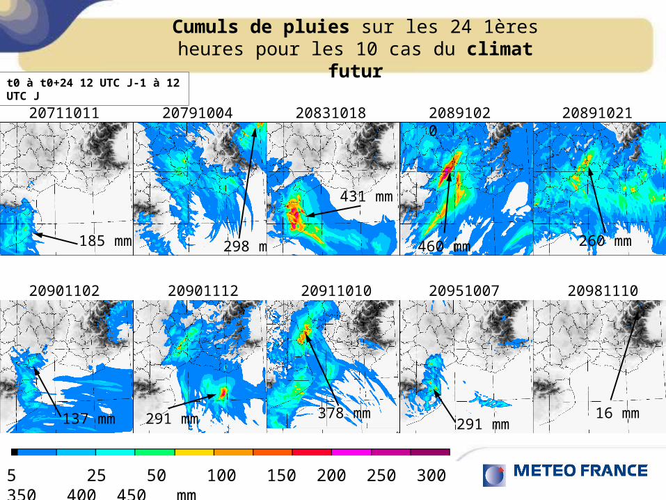
20711011

185 mm

20791004

298 mm

20911010

378 mm

20891020

460 mm

20891021

260 mm

20901102

137 mm

20831018

431 mm

20901112

291 mm

Cumuls de pluies sur les 24 1ères heures pour les 10 cas du climat futur

16 mm

20981110

291 mm

20951007

t0 à t0+24 12 UTC J-1 à 12 UTC J

5 25 50 100 150 200 250 300 350 400 450 mm

Diagnostics

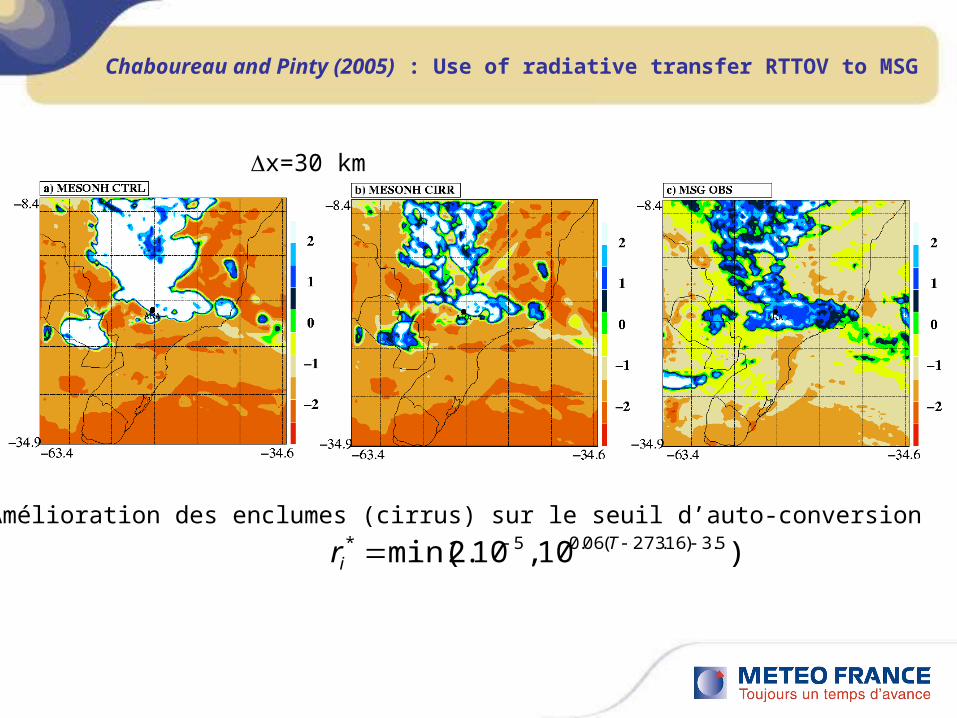
Chaboureau and Pinty (2005) : Use of radiative transfer RTTOV to MSG

x=30 km

Amélioration des enclumes (cirrus) sur le seuil d’auto-conversion

)10,10.2min( 5.3)16.273(06.05* Tir

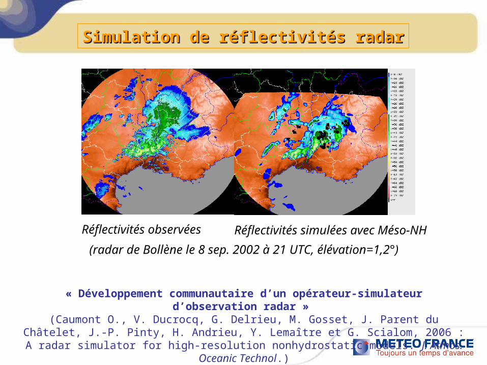
Réflectivités observées Réflectivités simulées avec Méso-NH

(radar de Bollène le 8 sep. 2002 à 21 UTC, élévation=1,2°)

« Développement communautaire d’un opérateur-simulateur d’observation radar »

(Caumont O., V. Ducrocq, G. Delrieu, M. Gosset, J. Parent du Châtelet, J.-P. Pinty, H. Andrieu, Y. Lemaître et G. Scialom, 2006 : A radar simulator for high-resolution

nonhydrostatic models. J. Atmos. Oceanic Technol.)

Simulation de réflectivités radarSimulation de réflectivités radar