1

MESMER: An open-source Master Equation Solver for Multi-Energy well Reactions

David R. Glowacki,a* Chi-Hsiu Liang, Christopher Morley, Michael J.

Pilling, and Struan H. Robertson*†

School of Chemistry, University of Leeds, Leeds LS2 9JT, UK

aSchool of Chemistry, University of Bristol, Bristol BS8 1TS, UK

†Accelrys Ltd., 334 Cambridge Science Park, Cambridge, CB4 0WN, UK

*drglowacki@gmail.com; struanr@accelrys.com

Abstract The most commonly used theoretical models for describing chemical kinetics are accurate in

two limits. When relaxation is fast with respect to reaction timescales, thermal transition state

theory (TST) is the theoretical tool of choice. In the limit of slow relaxation, an energy

resolved description like RRKM theory is more appropriate. For intermediate relaxation

regimes, where much of the chemistry in nature occurs, theoretical approaches are somewhat

less well established. However, in recent years master equation approaches have been

successfully used to analyze and predict non-equilibrium chemical kinetics across a range of

intermediate relaxation regimes spanning atmospheric, combustion, and (very recently)

solution phase organic chemistry. In this paper, we describe MESMER, a user-friendly,

object-oriented, open-source code designed to facilitate kinetic simulations over multi-well

molecular energy topologies where energy transfer with an external bath impacts

phenomenological kinetics. MESMER offers users a range of user options specified via

keywords, and also includes some unique statistical mechanics approaches like contracted

basis set methods and non-adiabatic RRKM theory for modelling spin-hopping. It is our hope

that the design principles implemented in MESMER will facilitate its development and usage

by workers across a range of fields concerned with chemical kinetics. As accurate

thermodynamics data becomes more widely available, electronic structure theory is

increasingly reliable, and our fundamental understanding of energy transfer improves, we

envision that tools like MESMER will eventually enable routine and reliable prediction of

non-equilibrium kinetics in arbitrary systems.

2

Introduction

The treatment of kinetic rate coefficients in a range of physical, environmental,

industrial, astrophysical, and biological systems is largely based on equilibrium statistical

mechanics – i.e., on Gibbs energies. In this regime, thermal relaxation timescales are much

faster than kinetic timescales, and canonical transition state theory (CTST) combined with

accurate molecular energies offers a reliable way to calculate rate coefficients.1 However, a

number of chemical reactions occur with non-equilibrium (i.e., non-Boltzmann) energy

distributions, giving rise to phenomenological kinetics that cannot be accurately described

using the machinery of equilibrium thermodynamics. In such regimes, free energy

descriptions are of limited value, often because the timescales for thermalization are

competitive with kinetic timescales. One successful theoretical approach for treating this

competition uses a stochastic energy grained master equation (EGME). The EGME typically

involves the calculation of energy resolved rate coefficients using microcanonical transition

state theory (µTST) and collisional energy transfer models. These are combined to construct a

model describing phenomenological rate coefficients that arise from competition between

reaction and thermalization of non-equilibrium ensembles. This approach has proven

successful in the gas phase – particularly in combustion chemistry and atmospheric chemistry.

Recently, the EGME has even been extended to resolve the microscopic details of non-

equilibrium kinetics occurring in solution phase synthetic organic chemistry.2,3

Generally speaking, the phenomenological quantities of particular interest in kinetic

modelling – e.g., for use in process models – include rate coefficients, time dependent species

profiles, product yields and reaction channel branching ratios. Each of these typically show a

complex dependence on pressure and temperature. One reason for the utility of the EGME is

that many industrial and environmental processes take place at temperatures and/or pressures

that are difficult to access in experimental studies of elementary reactions. The EGME is a

practical theoretical tool that allows one to optimize kinetic parameters at experimentally

accessible conditions, and subsequently predict kinetics in experimentally inaccessible

regimes. For example, experimental kinetics measurements of chemical reactions important in

combustion are performed at temperatures and pressures that are typically much lower than

those of real combustion systems. Similarly, experimental measurements of atmospheric

systems typically occur at pressures much lower than those relevant in the atmosphere. In

3

such cases, the EGME provides a quantitative means of extrapolating results obtained under

laboratory conditions to “realistic” conditions. A similar situation arises not only in

combustion and atmospheric chemistry, but also for interstellar chemistry and industrial

chemistry. In principle the EGME – in conjunction with µTST, scattering theory, and ab intio

calculations of a reactive system’s potential energy surface (PES) – is capable of providing a

first principles estimate of rate coefficients as a function of temperature and pressure.4-15

In this paper, we introduce MESMER, a Master Equation Solver for Multi-Energy

well Reactions. MESMER is a recently developed cross-platform, open-source software

project (see http://sourceforge.net/projects/mesmer/) which uses matrix techniques to

formulate and solve the EGME for unimolecular systems composed of an arbitrary number of

wells, transition states, sinks, and reactants. It offers a flexible approach to EGME treatments

of complex reactive systems and provides a complementary approach to stochastic simulation

programs such as Multiwell which utilize kinetic Monte-Carlo approaches.16,17 In developing

MESMER, we have also attempted to incorporate various facilities that make it easy to use

the EGME to directly interpret experimental observables. There are two principal design

goals that we have emphasized while writing MESMER. First, we use standard, off-the-shelf

technologies, so that the code may be readily maintained and extended. For example,

MESMER development has been facilitated by using the Microsoft Visual Studio and Xcode

integrated development environments (IDEs), XML data representation for the input stream,

and Firefox as a graphical user interface (GUI) to aid in constructing input files and

interpreting output files. Current developments are underway to increase compatibility

between MESMER and other open source projects as OpenBabel. Second, we have used open

source C++ to write structured, object-oriented, cross-platform code with the intent that it will

be easy to maintain and extend by future developers. Where possible, we have emphasized

plug-in classes to accommodate future developments in several different parts of the code –

e.g. partition function treatments, collisional energy transfer models, calculation of

microcanonical rate coefficients, and fitting of experimental data.

This paper is structured as follows: in section one we present an overview of the

theory of master equations (ME) as applied to gas phase reactions. In section two we discuss

in further detail some of the design principles we have adopted in developing MESMER.

Section three gives a more detailed discussion of some of MESMER’s features, with

particular attention to those features unique to MESMER. In section four, we discuss several

published examples where we have applied MESMER. Concluding remarks and an outlook

are given in section five.

4

1. The Energy Grained Master Equation: Theory

The form of the EGME discussed in this work is the one-dimensional ME, wherein the

total rovibrational energy of the system, E, is the independent variable. Indeed, a more

thorough treatment would not only consider the time dependent evolution of the system with

respect to the total energy, E, but also the angular momentum, J, as both of are constants of

motion.18 However, two-dimensional ME treatments (i.e., in terms of E and J) are restricted in

their application, given the difficulty of describing the transition probabilities wherein both E

and J are coupled. Presently, 2D approaches may only be used to solve the ME in the

collisionless limit,12,13 or for a system that has a single potential well.19 Thus, the bulk of ME

modelling on systems relevant to atmospheric and combustion chemistry is restricted to a J

averaged 1D ME,20,21 for which MESMER has been designed. In general, the 1D ME gives

reliable results and consequently it has been adopted by a number of workers. Part of the

reason for this is because the errors in molecular properties (e.g., energies and frequencies)

and experimental measurements (e.g., of rate coefficients or product yields) tend to have more

of an impact on ME results than those errors which are introduced by neglecting J.

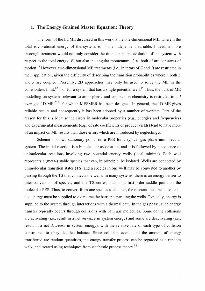
Scheme 1 shows stationary points on a PES for a typical gas phase unimolecular

system. The initial reaction is a bimolecular association, and it is followed by a sequence of

unimolecular reactions involving two potential energy wells (local minima). Each well

represents a (meta-) stable species that can, in principle, be isolated. Wells are connected by

unimolecular transition states (TS) and a species in one well may be converted to another by

passing through the TS that connects the wells. In many systems, there is an energy barrier to

inter-conversion of species, and the TS corresponds to a first-order saddle point on the

molecular PES. Thus, to convert from one species to another, the reactant must be activated –

i.e., energy must be supplied to overcome the barrier separating the wells. Typically, energy is

supplied to the system through interactions with a thermal bath. In the gas phase, such energy

transfer typically occurs through collisions with bath gas molecules. Some of the collisions

are activating (i.e., result in a net increase in system energy) and some are deactivating (i.e.,

result in a net decrease in system energy), with the relative rate of each type of collision

constrained to obey detailed balance. Since collision events and the amount of energy

transferred are random quantities, the energy transfer process can be regarded as a random

walk, and treated using techniques from stochastic process theory.8,9

5

Scheme 1. Representation of the Energy Grained Master Equation model for an association reaction (i.e., source term) with two wells, C1 and C2 and an irreversible product channel

The aim of the EGME is to provide a macroscopic kinetic description of a reaction

system, such as that shown in Scheme 1, in terms of the behaviour of each of the isomers at

an energy resolved (or microcanonical) level. At those energies which are typically significant

for describing non-equilibrium kinetics, the number of states in polyatomic molecules tends to

be very large, and describing the time evolution of every individual state represents an

impossibly expensive computational challenge. The EGME circumvents this problem by

bundling together rovibrational states of similar energies into ‘grains’, and then describing the

time evolution between these energy grains, which generally span no more than a few kJ mol-

1. The formulation of the EGME in terms of grains essentially corresponds to expanding the

solutions in a basis of delta functions whose origins lie at the centre of each grain.

Letting subscript m denote the index of a particular isomer on a reactive PES (e.g., for

Scheme 1 where there are two isomers, m∈1,2) and letting E denote the energy of a particular

grain, the rovibrational population density within a particular energy grain, pm(E), may be

described by a differential rate equation that accounts for collisional energy transfer within

each isomer as well reactive processes that both increase and decrease the grain population:

6

€

dpm (E)dt

=ω P(E | E ')pm (E ')dE 'E0m

∞

∫ − ωpm (E)

+ kmn (E)pn (E)n≠m

M

∑ − knm (E)pm (E)n≠m

M

∑

−kSm (E)pm (E)

+KRmeq kRm (E) ρm (E)e−βE

Qm (β)nA pB − kRm (E)pm (E)

(1)

The right hand side (RHS) of Eq (1) has seven terms. Three are positive, corresponding

to population flux into pm(E), and four are negative, corresponding to population flux out of

pm(E). The first term on the RHS of Eq. (1) describes population gain in pm(E) – i.e., isomer

Cm at energy E – via collisional energy transfer from other energy grains in that isomer. ω is

the Lennard-Jones collision frequency, and P(E|E’) is the probability that collision with bath

gas will result in a transition from a grain with energy E’ to a grain with energy E. The second

term represents population loss from grain pm(E) via collisional energy transfer. The third

term describes reversible population gain into grain pm(E) by reactions that transfer

population from isomer n to isomer m at a particular energy E (kmn(E) is the microcanonical

rate constant for population transfer from grains in isomer n to grains in isomer m). The fourth

term describes reversible population loss from pm(E) via reactions that transfer population

from grains in isomer m to the other possible isomers, denoted by index n (knm(E) are the

microcanonical rate coefficients for population transfer from isomer m to isomer n at energy

E). The fifth term describes irreversible population loss from pm(E) via reactions that transfer

population from isomer m to products S with microcanonical rate coefficient kSm(E). The

inclusion of such irreversible loss terms introduces an infinite sink approximation, and

consequently requires careful consideration when implemented in Eq. (1).10,22 In general,

infinite sink approximations are reasonable in two different scenarios: (i) for unimolecular

dissociation processes, so long as re-association timescales are much longer than the

phenomenological kinetic timescales under consideration, which is often the case under a

range of conditions, e.g. where the concentration of one of the co-reactants in the product set

S is negligible; and (ii) for unimolecular isomerizations with an exceptionally large reverse

barrier, where the magnitude of the backward rate coefficient, kmn(E), is negligible compared

to the forward rate coefficient, knm(E).

The final two terms in Eq. (1) pertain to the so-called bimolecular source term, and

7

apply only to those isomers that are populated via bimolecular association reactions (e.g., well

C1 in Scheme 1). Assuming (i) that the bimolecular reactants, A and B, are maintained in a

Boltzmann distribution on the phenomenological timescale of interest, and (ii) that reactant A

is in significant excess compared to reactant B (i.e., [A] >> [B]), and a pseudo-first order

kinetics approximation is therefore appropriate, then the sixth and seventh terms respectively

describe population gain in pm(E) from association of reactants A and B (together denoted as

R), and population loss from pm(E) via re-dissociation to reactants. kRm(E) represents the rate

constant at which pm(E) re-dissociates to give the bimolecular reactants, R, and is the

equilibrium constant between isomer m and the reactants.

€

Qm (β) = dEρm (E)e−βE∫ , which

is the rovibrational partition function for the molecular species corresponding to isomer m, nA

is the number density of reactant A, and pB is the population in reactant B.9,13

Eq. (1) as written does not represent a closed system of differential equations

because pB is unspecified. In the cases where a bimolecular association reaction is to be

included in a reaction network (e.g., in Scheme 1) then an additional differential equation

must be included to describe the time dependence of pB:

(2)

Over the entire set of energy grains and isomers, Equations (1) and (2) give a set of

coupled ordinary differential equations that may be solved using stochastic approaches like

kinetic Monte-Carlo16,17,23 or matrix diagonalization techniques.24 The advantage of using

matrix techniques is the availability of techniques (discussed below) that allow us to solve Eq

(1) and (2) directly, and relate their eigenvalues and eigenvectors to temperature and pressure

dependent phenomenological rate coefficients of the sorts observed by experimentalists – i.e.,

the sort of data generally required as input for kinetic mechanisms of combustion and

atmospheric chemistry. The disadvantage of using matrix techniques is that there are certain

situations (also discussed below) in which numerical instabilities arise, giving unreliable

eigenvectors and eigenvalues.25,26

In setting up the matrix form of Eq. (1) and (2), the energy grains of the different

isomers are concatenated and then indexed using a single index, i, that labels the grains of all

of the isomers. The coupled set of differential equations may then be expressed as:

8

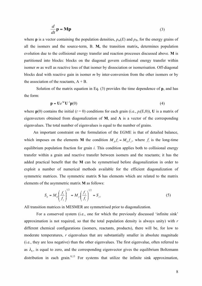
(3)

where p is a vector containing the population densities, pm(E) and pB, for the energy grains of

all the isomers and the source-term, B. M, the transition matrix, determines population

evolution due to the collisional energy transfer and reaction processes discussed above. M is

partitioned into blocks: blocks on the diagonal govern collisional energy transfer within

isomer m as well as reactive loss of that isomer by dissociation or isomerisation. Off-diagonal

blocks deal with reactive gain in isomer m by inter-conversion from the other isomers or by

the association of the reactants, A + B.

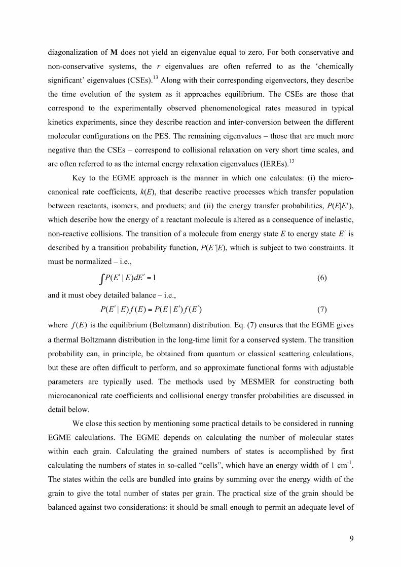
Solution of the matrix equation in Eq. (3) provides the time dependence of p, and has

the form:

(4)

where p(0) contains the initial (t = 0) conditions for each grain (i.e., pi(E,0)), U is a matrix of

eigenvectors obtained from diagonalization of M, and is a vector of the corresponding

eigenvalues. The total number of eigenvalues is equal to the number of grains.

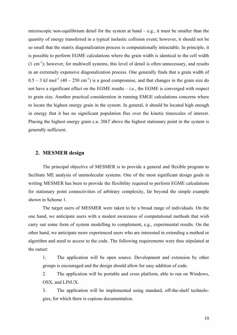
An important constraint on the formulation of the EGME is that of detailed balance,

which imposes on the elements M the condition

€

M ji f i = Mij f j , where is the long-time

equilibrium population fraction for grain i. This condition applies both to collisional energy

transfer within a grain and reactive transfer between isomers and the reactants; it has the

added practical benefit that the M can be symmetrised before diagonalization in order to

exploit a number of numerical methods available for the efficient diagonalization of

symmetric matrices. The symmetric matrix S has elements which are related to the matrix

elements of the asymmetric matrix M as follows:

(5)

All transition matrices in MESMER are symmetrised prior to diagonalization.

For a conserved system (i.e., one for which the previously discussed ‘infinite sink’

approximation is not required, so that the total population density is always unity) with r

different chemical configurations (isomers, reactants, products), there will be, for low to

moderate temperatures, r eigenvalues that are substantially smaller in absolute magnitude

(i.e., they are less negative) than the other eigenvalues. The first eigenvalue, often referred to

as , is equal to zero, and the corresponding eigenvector gives the equilibrium Boltzmann

distribution in each grain.8,13 For systems that utilize the infinite sink approximation,

9

diagonalization of M does not yield an eigenvalue equal to zero. For both conservative and

non-conservative systems, the r eigenvalues are often referred to as the ‘chemically

significant’ eigenvalues (CSEs).13 Along with their corresponding eigenvectors, they describe

the time evolution of the system as it approaches equilibrium. The CSEs are those that

correspond to the experimentally observed phenomenological rates measured in typical

kinetics experiments, since they describe reaction and inter-conversion between the different

molecular configurations on the PES. The remaining eigenvalues – those that are much more

negative than the CSEs – correspond to collisional relaxation on very short time scales, and

are often referred to as the internal energy relaxation eigenvalues (IEREs).13

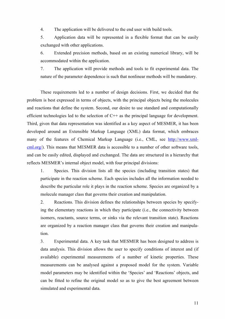
Key to the EGME approach is the manner in which one calculates: (i) the micro-

canonical rate coefficients, k(E), that describe reactive processes which transfer population

between reactants, isomers, and products; and (ii) the energy transfer probabilities, P(E|E’),

which describe how the energy of a reactant molecule is altered as a consequence of inelastic,

non-reactive collisions. The transition of a molecule from energy state E to energy state is

described by a transition probability function, P(E’|E), which is subject to two constraints. It

must be normalized – i.e.,

(6)

and it must obey detailed balance – i.e.,

(7)

where is the equilibrium (Boltzmann) distribution. Eq. (7) ensures that the EGME gives

a thermal Boltzmann distribution in the long-time limit for a conserved system. The transition

probability can, in principle, be obtained from quantum or classical scattering calculations,

but these are often difficult to perform, and so approximate functional forms with adjustable

parameters are typically used. The methods used by MESMER for constructing both

microcanonical rate coefficients and collisional energy transfer probabilities are discussed in

detail below.

We close this section by mentioning some practical details to be considered in running

EGME calculations. The EGME depends on calculating the number of molecular states

within each grain. Calculating the grained numbers of states is accomplished by first

calculating the numbers of states in so-called “cells”, which have an energy width of 1 cm-1.

The states within the cells are bundled into grains by summing over the energy width of the

grain to give the total number of states per grain. The practical size of the grain should be

balanced against two considerations: it should be small enough to permit an adequate level of

10

microscopic non-equilibrium detail for the system at hand – e.g., it must be smaller than the

quantity of energy transferred in a typical inelastic collision event; however, it should not be

so small that the matrix diagonalization process is computationally intractable. In principle, it

is possible to perform EGME calculations where the grain width is identical to the cell width

(1 cm-1); however, for multiwell systems, this level of detail is often unnecessary, and results

in an extremely expensive diagonalization process. One generally finds that a grain width of

0.5 – 3 kJ mol-1 (40 – 250 cm-1) is a good compromise, and that changes in the grain size do

not have a significant effect on the EGME results – i.e., the EGME is converged with respect

to grain size. Another practical consideration in running EMGE calculations concerns where

to locate the highest energy grain in the system. In general, it should be located high enough

in energy that it has no significant population flux over the kinetic timescales of interest.

Placing the highest energy grain c.a. 20kT above the highest stationary point in the system is

generally sufficient.

2. MESMER design

The principal objective of MESMER is to provide a general and flexible program to

facilitate ME analysis of unimolecular systems. One of the most significant design goals in

writing MESMER has been to provide the flexibility required to perform EGME calculations

for stationary point connectivities of arbitrary complexity, far beyond the simple example

shown in Scheme 1.

The target users of MESMER were taken to be a broad range of individuals. On the

one hand, we anticipate users with a modest awareness of computational methods that wish

carry out some form of system modelling to complement, e.g., experimental results. On the

other hand, we anticipate more experienced users who are interested in extending a method or

algorithm and need to access to the code. The following requirements were thus stipulated at

the outset:

1. The application will be open source. Development and extension by other

groups is encouraged and the design should allow for easy addition of code.

2. The application will be portable and cross platform, able to run on Windows,

OSX, and LINUX.

3. The application will be implemented using standard, off-the-shelf technolo-

gies, for which there is copious documentation.

11

4. The application will be delivered to the end user with build tools.

5. Application data will be represented in a flexible format that can be easily

exchanged with other applications.

6. Extended precision methods, based on an existing numerical library, will be

accommodated within the application.

7. The application will provide methods and tools to fit experimental data. The

nature of the parameter dependence is such that nonlinear methods will be mandatory.

These requirements led to a number of design decisions. First, we decided that the

problem is best expressed in terms of objects, with the principal objects being the molecules

and reactions that define the system. Second, our desire to use standard and computationally

efficient technologies led to the selection of C++ as the principal language for development.

Third, given that data representation was identified as a key aspect of MESMER, it has been

developed around an Extensible Markup Language (XML) data format, which embraces

many of the features of Chemical Markup Language (i.e., CML, see http://www.xml-

cml.org/). This means that MESMER data is accessible to a number of other software tools,

and can be easily edited, displayed and exchanged. The data are structured in a hierarchy that

reflects MESMER’s internal object model, with four principal divisions:

1. Species. This division lists all the species (including transition states) that

participate in the reaction scheme. Each species includes all the information needed to

describe the particular role it plays in the reaction scheme. Species are organized by a

molecule manager class that governs their creation and manipulation.

2. Reactions. This division defines the relationships between species by specify-

ing the elementary reactions in which they participate (i.e., the connectivity between

isomers, reactants, source terms, or sinks via the relevant transition state). Reactions

are organized by a reaction manager class that governs their creation and manipula-

tion.

3. Experimental data. A key task that MESMER has been designed to address is

data analysis. This division allows the user to specify conditions of interest and (if

available) experimental measurements of a number of kinetic properties. These

measurements can be analysed against a proposed model for the system. Variable

model parameters may be identified within the ‘Species’ and ‘Reactions’ objects, and

can be fitted to refine the original model so as to give the best agreement between

simulated and experimental data.

12

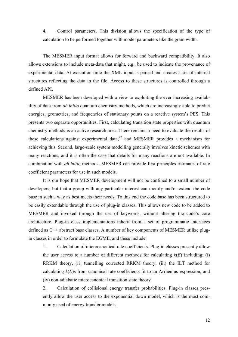
4. Control parameters. This division allows the specification of the type of

calculation to be performed together with model parameters like the grain width.

The MESMER input format allows for forward and backward compatibility. It also

allows extensions to include meta-data that might, e.g., be used to indicate the provenance of

experimental data. At execution time the XML input is parsed and creates a set of internal

structures reflecting the data in the file. Access to these structures is controlled through a

defined API.

MESMER has been developed with a view to exploiting the ever increasing availab-

ility of data from ab initio quantum chemistry methods, which are increasingly able to predict

energies, geometries, and frequencies of stationary points on a reactive system’s PES. This

presents two separate opportunities. First, calculating transition state properties with quantum

chemistry methods is an active research area. There remains a need to evaluate the results of

these calculations against experimental data,22 and MESMER provides a mechanism for

achieving this. Second, large-scale system modelling generally involves kinetic schemes with

many reactions, and it is often the case that details for many reactions are not available. In

combination with ab initio methods, MESMER can provide first principles estimates of rate

coefficient parameters for use in such models.

It is our hope that MESMER development will not be confined to a small number of

developers, but that a group with any particular interest can modify and/or extend the code

base in such a way as best meets their needs. To this end the code base has been structured to

be easily extendable through the use of plug-in classes. This allows new code to be added to

MESMER and invoked through the use of keywords, without altering the code’s core

architecture. Plug-in class implementations inherit from a set of programmatic interfaces

defined as C++ abstract base classes. A number of key components of MESMER utilize plug-

in classes in order to formulate the EGME, and these include:

1. Calculation of microcanonical rate coefficients. Plug-in classes presently allow

the user access to a number of different methods for calculating k(E) including: (i)

RRKM theory, (ii) tunnelling corrected RRKM theory, (iii) the ILT method for

calculating k(E)s from canonical rate coefficients fit to an Arrhenius expression, and

(iv) non-adiabatic microcanonical transition state theory.

2. Calculation of collisional energy transfer probabilities. Plug-in classes pres-

ently allow the user access to the exponential down model, which is the most com-

monly used of energy transfer models.

13

3. Calculation of rovibrational densities of states (DOS) for isomers, reactants,

products, and transition states. Plug-in classes offer a number of different approaches

for calculating both external and internal rotational DOS. MESMER can calculate

external DOS using both classical and quantum partition functions for linear, spher-

ical, symmetric and asymmetric tops. For internal rotations, MESMER includes a

method to calculate the DOS for a quantum mechanical hindered rotor (discussed

below).

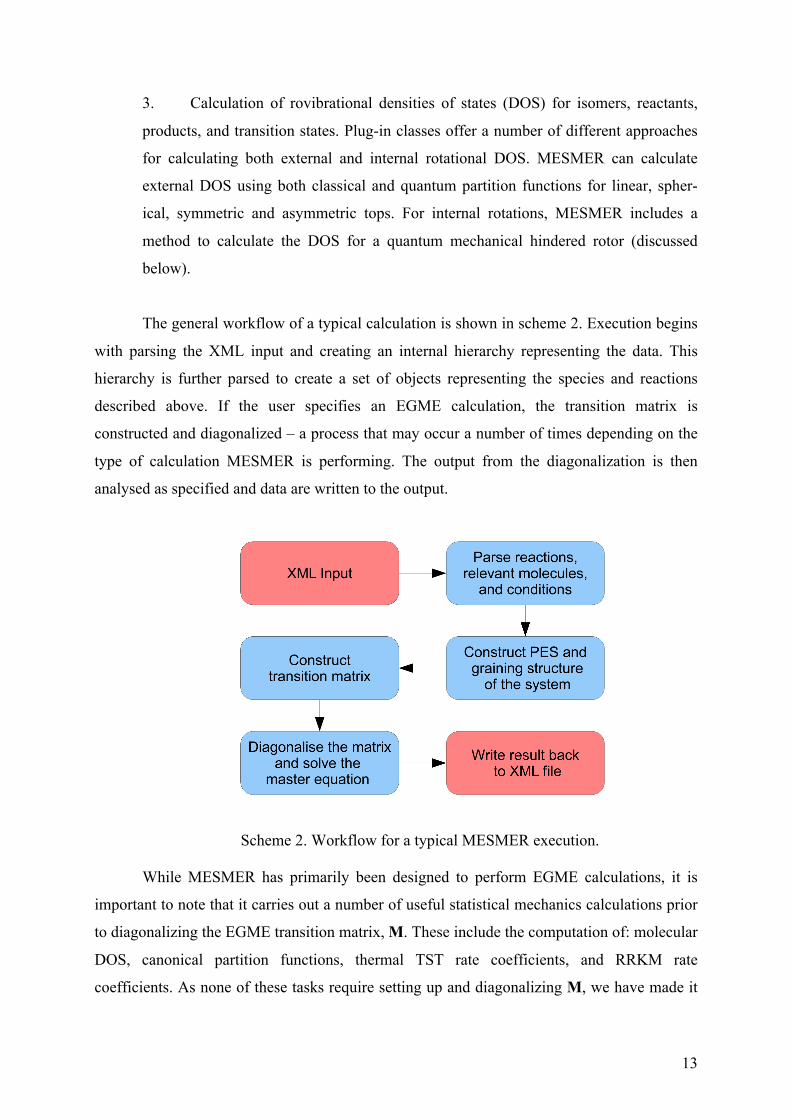
The general workflow of a typical calculation is shown in scheme 2. Execution begins

with parsing the XML input and creating an internal hierarchy representing the data. This

hierarchy is further parsed to create a set of objects representing the species and reactions

described above. If the user specifies an EGME calculation, the transition matrix is

constructed and diagonalized – a process that may occur a number of times depending on the

type of calculation MESMER is performing. The output from the diagonalization is then

analysed as specified and data are written to the output.

Scheme 2. Workflow for a typical MESMER execution.

While MESMER has primarily been designed to perform EGME calculations, it is

important to note that it carries out a number of useful statistical mechanics calculations prior

to diagonalizing the EGME transition matrix, M. These include the computation of: molecular

DOS, canonical partition functions, thermal TST rate coefficients, and RRKM rate

coefficients. As none of these tasks require setting up and diagonalizing M, we have made it

14

possible for users to specify that MESMER perform these tasks without solving the full

EGME.

MESMER’s primary output channel is via the internal data structures created during

the initial parsing of the input XML. Calculated data are added to these data structures and all

data are persisted at the conclusion of the execution, so that a calculation can be restarted

from where it terminated: any datafile can be used as input. There are two other output files: a

*.log file which reports the progress of the calculation and logs messages reported during

execution, and a *.test file which is used to record more detailed data, often for the purposes

of debugging and quality control. Important errors are shown on the console.

At present MESMER is a command line application. However, having the data files in

XML format allows them to be edited, visualized and analyzed by external programs. For

example, MESMER is currently distributed along with an XSLT stylesheet that transforms

the XML to HTML and SVG for displaying input data in Firefox (or another browser). This

gives a text display that organizes the data in an easy-to-view and user-friendly form, showing

important input properties of the species and reactions, as well as output results. The XSLT is

also used to construct diagrams: it shows the reaction potential energy surface as well as plots

of output data (e.g., time-dependent species profiles and phenomenological rate coefficients).

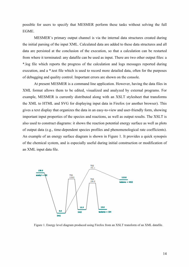
An example of an energy surface diagram is shown in Figure 1. It provides a quick synopsis

of the chemical system, and is especially useful during initial construction or modification of

an XML input data file.

Figure 1. Energy level diagram produced using Firefox from an XSLT transform of an XML datafile.

15

3. Current implementation details

In this section, we provide an overview of several of the methods and features avail-

able in MESMER, paying particular attention to those capabilities that, to our knowledge, are

unique to MESMER.

3.1. DOS treatment

Within MESMER, rovibrational DOS are evaluated on the assumption that the rota-

tional DOS are separable from vibrational DOS, which is a good approximation at low

energies. There are a number of models for evaluating molecular densities of states, and to

accommodate these, MESMER has an abstract interface that allows a new model to be added

via a plug-in class. At present MESMER calculates vibrational DOS using the Beyer-

Swinehart algorithm in conjunction with a harmonic oscillator approximation.27 A number of

plugin class options are available for calculating the rotational DOS of both external and

internal rotors, and are detailed below.

3.1.1. Classical and Quantum Mechanical external rotors

MESMER presently treats external rotors as rigid. This approximation is most reason-

able for systems with small numbers of atoms. For larger systems the approximation may be

less applicable, as the coupling strength between large-amplitude internal motions and

external rotation increases – i.e., the moments of inertia can depend on an internal rotor

degree of freedom and there may be significant Coriolis coupling.28 However, the detailed

calculation of these coupling terms is a complex exercise and progress has been largely

confined to approaches based on classical mechanics. With a statistical state counting

approach, the details of individual states are less important than the number of states within a

given energy range, and a rigid rotor approximation often gives a reasonable description of

this state distribution. MESMER treats internal and external rotational symmetry using

symmetry numbers in the standard way.29

MESMER offers a classical and a quantum mechanical (QM) plug-in class with a

number of methods for different types of rotors.27 Details are given in table 1. Each method

returns an array which includes the state densities calculated using either a classical

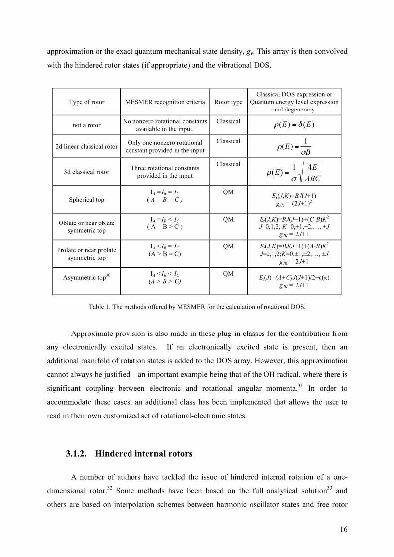
16

approximation or the exact quantum mechanical state density, gv. This array is then convolved

with the hindered rotor states (if appropriate) and the vibrational DOS.

Table 1. The methods offered by MESMER for the calculation of rotational DOS.

Approximate provision is also made in these plug-in classes for the contribution from

any electronically excited states. If an electronically excited state is present, then an

additional manifold of rotation states is added to the DOS array. However, this approximation

cannot always be justified – an important example being that of the OH radical, where there is

significant coupling between electronic and rotational angular momenta.31 In order to

accommodate these cases, an additional class has been implemented that allows the user to

read in their own customized set of rotational-electronic states.

3.1.2. Hindered internal rotors

A number of authors have tackled the issue of hindered internal rotation of a one-

dimensional rotor.32 Some methods have been based on the full analytical solution33 and

others are based on interpolation schemes between harmonic oscillator states and free rotor

Type of rotor MESMER recognition criteria Rotor type Classical DOS expression or

Quantum energy level expression and degeneracy

not a rotor No nonzero rotational constants available in the input.

Classical

2d linear classical rotor Only one nonzero rotational constant provided in the input

Classical

3d classical rotor Three rotational constants provided in the input

Classical

Spherical top IA =IB = IC

( A = B = C )

QM Er(J,K)=BJ(J+1) gJK = (2J+1)2

Oblate or near oblate symmetric top

IA =IB < IC ( A = B > C )

QM Er(J,K)=BJ(J+1)+(C-B)K2

J=0,1,2; K=0,±1,±2,…, ±J gJK = 2J+1

Prolate or near prolate symmetric top

IA <IB = IC (A > B = C)

QM Er(J,K)=BJ(J+1)+(A-B)K2

J=0,1,2;K=0,±1,±2,…, ±J gJK = 2J+1

Asymmetric top30

IA <IB < IC (A > B > C)

QM Er(J)=(A+C)J(J+1)/2+ε(κ) gJK = 2J+1

17

states.34 Here an approached is presented based on the expansion of the one-dimensional

hindered rotor Hamiltonian in terms of the free rotor wave functions, which follows closely

the development given by Lewis et al.35 This approach has been implemented within

MESMER as it allows consideration of more complex potentials, such as might be obtained

from ab initio investigations.

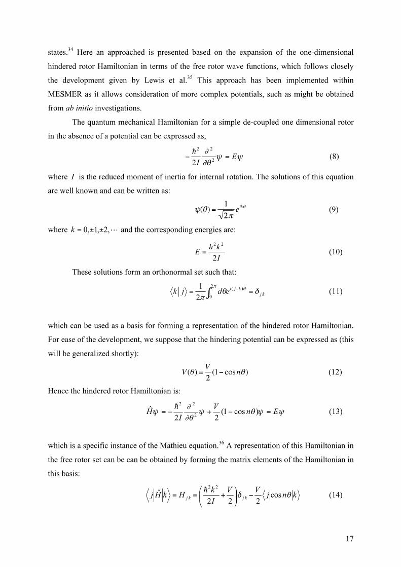
The quantum mechanical Hamiltonian for a simple de-coupled one dimensional rotor

in the absence of a potential can be expressed as,

(8)

where is the reduced moment of inertia for internal rotation. The solutions of this equation

are well known and can be written as:

(9)

where and the corresponding energies are:

(10)

These solutions form an orthonormal set such that:

(11)

which can be used as a basis for forming a representation of the hindered rotor Hamiltonian.

For ease of the development, we suppose that the hindering potential can be expressed as (this

will be generalized shortly):

(12)

Hence the hindered rotor Hamiltonian is:

(13)

which is a specific instance of the Mathieu equation.36 A representation of this Hamiltonian in

the free rotor set can be can be obtained by forming the matrix elements of the Hamiltonian in

this basis:

(14)

18

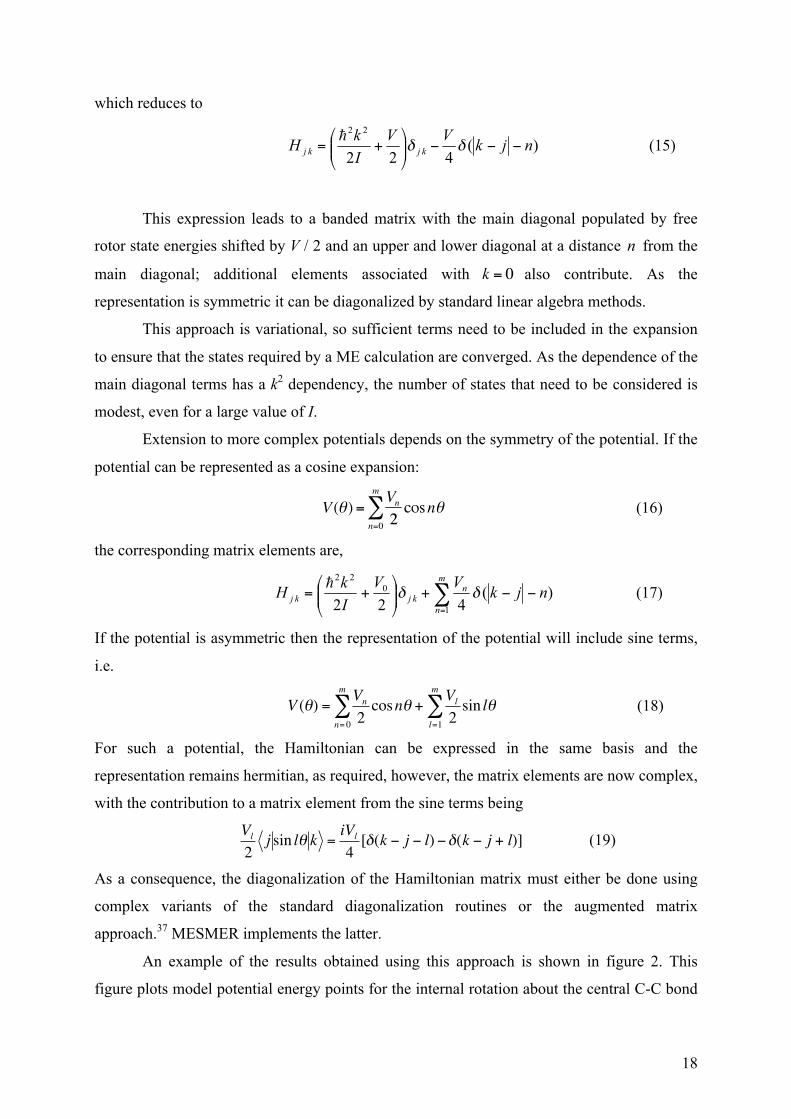
which reduces to

(15)

This expression leads to a banded matrix with the main diagonal populated by free

rotor state energies shifted by V / 2 and an upper and lower diagonal at a distance from the

main diagonal; additional elements associated with also contribute. As the

representation is symmetric it can be diagonalized by standard linear algebra methods.

This approach is variational, so sufficient terms need to be included in the expansion

to ensure that the states required by a ME calculation are converged. As the dependence of the

main diagonal terms has a k2 dependency, the number of states that need to be considered is

modest, even for a large value of I.

Extension to more complex potentials depends on the symmetry of the potential. If the

potential can be represented as a cosine expansion:

(16)

the corresponding matrix elements are,

(17)

If the potential is asymmetric then the representation of the potential will include sine terms,

i.e.

€

V (θ) =Vn

2cosnθ

n= 0

m

∑ +Vl

2sin lθ

l=1

m

∑ (18)

For such a potential, the Hamiltonian can be expressed in the same basis and the

representation remains hermitian, as required, however, the matrix elements are now complex,

with the contribution to a matrix element from the sine terms being

€

Vl

2j sin lθ k =

iVl

4[δ(k − j − l) −δ(k − j + l)] (19)

As a consequence, the diagonalization of the Hamiltonian matrix must either be done using

complex variants of the standard diagonalization routines or the augmented matrix

approach.37 MESMER implements the latter.

An example of the results obtained using this approach is shown in figure 2. This

figure plots model potential energy points for the internal rotation about the central C-C bond

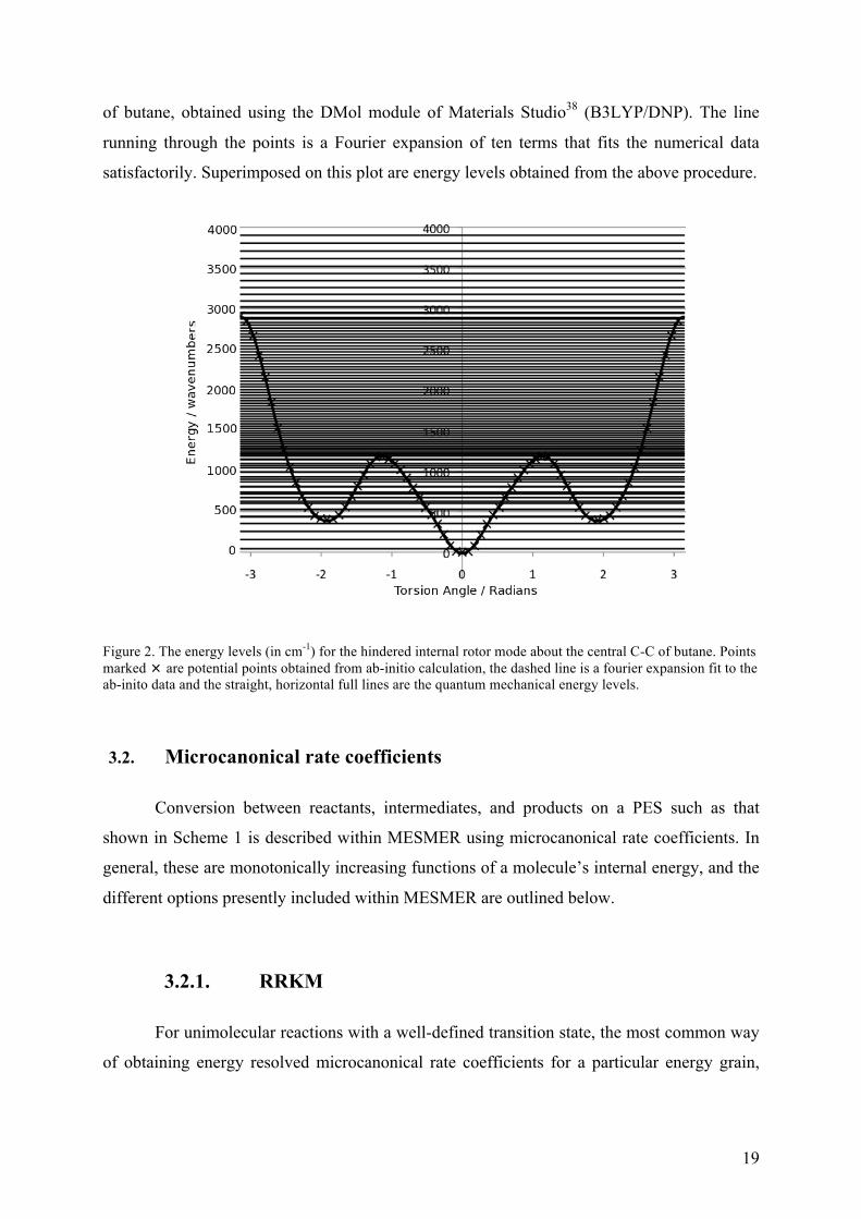
19

of butane, obtained using the DMol module of Materials Studio38 (B3LYP/DNP). The line

running through the points is a Fourier expansion of ten terms that fits the numerical data

satisfactorily. Superimposed on this plot are energy levels obtained from the above procedure.

Figure 2. The energy levels (in cm-1) for the hindered internal rotor mode about the central C-C of butane. Points marked are potential points obtained from ab-initio calculation, the dashed line is a fourier expansion fit to the ab-inito data and the straight, horizontal full lines are the quantum mechanical energy levels.

3.2. Microcanonical rate coefficients

Conversion between reactants, intermediates, and products on a PES such as that

shown in Scheme 1 is described within MESMER using microcanonical rate coefficients. In

general, these are monotonically increasing functions of a molecule’s internal energy, and the

different options presently included within MESMER are outlined below.

3.2.1. RRKM

For unimolecular reactions with a well-defined transition state, the most common way

of obtaining energy resolved microcanonical rate coefficients for a particular energy grain,

20

, utilizes RRKM theory, which is a microcanonical formulation of TST. The RRKM

expression is:8

(20)

where is the rovibrational sum of states (SOS) at the optimized transition state

(TS) geometry (excluding the degree of freedom associated with passage through the TS),

is the reaction threshold energy, h is Planck’s constant, and ρ(E) is the density of

rovibrational states of the reactant. RRKM theory depends on the assumption that the total

phase space of a molecule at a particular energy is uniformly populated as the molecule

passes from reactant to product through the transition state dividing surface, and the time

scale for energy randomization is very short compared with that of reaction, so that a

microcanonical ensemble is maintained.39,40 This is commonly called the ergodicity

assumption. The RRKM equation is applicable for transition state dividing surfaces located at

a constrained geometry with a well-defined energetic barrier. When the reaction in question

is barrierless, a first principles determination of requires a variational approach – i.e.,

is calculated by minimizing W(E) on the PES in question.41 This approach is not

currently available in MESMER; instead we use an approach using inverse Laplace

transformation (ILT), which is discussed in the following section.

3.2.2. Unimolecular and association ILT

An alternative to using the RRKM expression for calculating is to use an ILT.

With this technique, the unimolecular microcanonical is determined from either

experimental measurements or theoretical determinations of the canonical high pressure

limiting rate coefficient, k∞(T). So long as the forward k(T)s may be cast in the modified

Arrhenius form discussed below, then the relationship between k(E)s obtained from ILT and

the corresponding k(T)s is exact – i.e., the ILT method yields a set of forward k(E)s which,

when multiplied by a Boltzmann distribution and summed, give back the k(T)s. For an

isomerisation reaction, the microcanonical rate coefficients for the reverse reaction may be

straightforwardly determined via detailed balance. The ILT method for obtaining k(E) is

particularly well-suited to barrierless reactions, where conventional TST and RRKM theory

21

are not appropriate because the location of the transition state depends on energy, a situation

which is typical of radical-radical associations. In such cases, experimental determinations of

k∞(T) or sophisticated versions of VTST, such as flexible transition state theory (FTST),42,43

are generally far more accurate. So long as the canonical rate coefficients obtained from either

of these approaches can be fitted to an Arrhenius or modified Arrhenius form, then they may

be used to calculate accurate k(E)s via ILT. MESMER has two implementations of ILT – one

for unimolecular dissociation and isomerisation reactions, and one for association reactions.

The basis of the ILT methods is that canonical high pressure rate coefficient may be

expressed as:

€

k∞(β) =1

Q(β)k(E)ρ(E)exp(−βE)dE

0

∞

∫ (21)

where ρ(E) is the reactant rovibrational density of states and Q(β) is the corresponding

canonical partition function. Letting L denote a Laplace transform and rearranging gives:

(22)

If can be represented by the modified Arrhenius expression,

(23)

it follows that:

(24)

Further progress can be made by applying the convolution theorem, ,

where denotes convolution, with transform pairs Q, q and G, g. Solving the respective ILTs

for use in the convolution theorem gives

(25)

where u is the Heavyside step function. Subsequent convolution of these solutions gives:

22

(26)

where τ is a dummy integration variable.

A similar expression can be obtained for the case where the Arrhenius or modified

Arrhenius expression provides an accurate representation of the high pressure association rate

coefficient. The forward (association) and reverse (dissociation) rate coefficients are related

by the equilibrium constant, Ke(β), as follows:

€

kd∞(β) = Ke (β)ka

∞(β) (27)

where subscript a denotes association and subscript d dissociation If ka∞(β) can be represented

using a modified Arrhenius form, then for dissociation may be obtained using the

following ILT equation:

(28)

where the modified Arrhenius parameters now refer to the association rate coefficient.

Solving the above equation is complicated by some extra algebra that arises from translational

degrees of freedom in the equilibrium constant, but otherwise proceeds as above by exploiting

the convolution theorem. The final result (for a reaction of type A + B → C) is:44

(29)

where ρR(E) is the convolved density of states for the associating pair, is the enthalpy of

reaction, µ is the reduced mass of the system and gX is the spin degeneracy of species X.

3.2.3. Tunneling corrections

Tunnelling and non-classical reflection can be included within the standard RRKM

expression by a simple modification of the transition state sum of states as follows:45

(30)

23

where Wtunn(E) is a convolution of the tunnelling transmission probabilities, Ptunn(E), with

ρTS(E), the transition state DOS – i.e.:

(31)

where E0 is the classical barrier height in the direction of the forward reaction, ET is the

energy in the reaction coordinate relative to the top of the energy barrier, E is the total energy,

and the zero of energy is chosen to lie at the classical barrier. Presently, MESMER can

include tunnelling corrections through an asymmetric Eckart barrier, in which the tunnelling

transmission probabilities are calculated as follows:45

(32)

where vi is the imaginary frequency at the top of the barrier, and V1 is the classical barrier

height with respect to the products.

3.2.4. Non-adiabatic RRKM for spin hopping problem

MESMER also includes an implementation of microcanonical non-adiabatic transition

state theory (NA-TST), which is described in detail elsewhere.46 The manner in which NA-

TST is implemented is very similar to the method in which tunnelling corrections are

implemented, beginning with the typical RRKM expression, but replacing the sum of states at

the TS with the sum of states at the minimum energy crossing point (MECP) between the two

diabatic surfaces – i.e.:

(33)

where WMECP(E) is a convolution of the density of states at the MECP geometry, ,

and the spin forbidden hopping (SH) probabilities, PSH(E):

(34)

MESMER presently includes a Landau-Zener (LZ) spin hopping model,47,48 in which:

24

€

pSH (EH ) = (1+ P)(1− P)

P = exp −2πH122

hΔFµ

2(E − EMECP )

(35)

where corresponds to a double passage hopping probability with non-adiabatic

transit allowed on both forward and reverse passage through the MECP, H12 is the matrix

element for coupling between the two surfaces, µ is the reduced mass for movement along the

vector orthogonal to the singlet/triplet crossing seam, and ΔF is the relative slope of the two

surfaces at the crossing seam. The LZ surface hopping model is best suited to non-adiabatic

systems with localized coupling regions and narrowly avoided crossings. In Eq. (35), the hopping probabilities for energies below the MECP are zero. MES-

MER includes another method for treating LZ hopping, which additionally allows tunnelling

at energies below the MECP using an expression derived from a semiclassical WKB

approximation:49,50

€

pSH (EH ) = 4π 2H122 exp −2µ

2FΔF

2 / 3

Ai2 (E − EMECP )2µΔF 2

2F 4

1/ 3

(36)

where F is the average of the slopes on the two surfaces at the MECP, and Ai denotes the Airy

function.

3.3. Phenomenological rate coefficients

Solution of Eq. (3) yields the full microcanonical description of the system time

evolution – i.e., for every energy grain in the system. In general, however, this information is

more than what is required; one is often interested in the phenomenological rate coefficients

for the set of chemical reactions linking the reactants, adduct isomers and products, as well as

related quantities such as product yields and branching ratios. It is therefore important to

relate the microcanonical information contained in Eq. (3) to the phenomenological quantities

of interest. MESMER implements a procedure based upon that described by Bartis and

Widom51 which uses the eigenvectors and eigenvalues obtained from solution of Eq. (3) to

provide phenomenological rate coefficients for arbitrary interconnected networks of

stationary points.

The mathematical development of the Bartis-Widom technique implemented in

MESMER is described by Robertson et al.,10 and so will not be detailed here. Briefly, the

basic idea is as follows: for typical atmospheric and combustion systems, the phenomenologi-

25

cal time evolution for an arbitrarily interconnected kinetic system of molecular species is

typically described using a coupled set of differential equations, similar in form to those of

Eq. (3), with the difference that the population of each species is represented by a single term

in the population vector rather than a set of energy grains. Assuming that n species make up

the kinetic scheme, the coupled set of differential equations may be written using an n × n rate

coefficient matrix K representing n coupled first order or pseudo first order differential

equations:

(37)

where the matrix element Kab is the rate coefficient kb→a(T,P) for all possible reactions and c

is a vector of species concentrations. Diagonalization of this rate matrix yields a solution in

terms of n eigenvalues and n eigenvectors. The principle difference between M and K is that

the matrix elements of the latter do not include an explicit description of collisional

relaxation, which occurs on timescales much shorter than those which characterize

phenomenological kinetics.

The Bartis-Widom method exploits the separation between the internal energy relax-

ation eigenvalues (IEREs) and chemically significant eigenvalues (CSEs): assuming that the

CSEs obtained from the diagonalization of M (which explicitly include collisional relaxation)

are identical to those which could be obtained from diagonalization of K, then the n × n

phenomenological rate matrix K may be reconstructed from the CSEs using simple matrix

algebra. The Bartis-Widom analysis is a useful technique because it provides a global

description of the time dependent kinetics in terms of n × n rate coefficients, and in many

cases, the phenomenological rate coefficient is the quantity of interest to be obtained from a

ME calculation. However, the Bartis-Widom analysis relies on the separation between CSEs

and IEREs. If these are not well separated (practically speaking, by more than an order of

magnitude), the system cannot be represented by a set of first order rate equations linking the

concentrations of the n species in the vector c. This means that the rate coefficients provided

by the Bartis-Widom analysis are unreliable and MESMER will print a warning. In such

cases, and so long as numerical precision is not an issue, the user may rely on the species

profiles to analyse the system kinetics, since these do not require separation between CSEs

and IEREs. When there is good separation between the CSEs and the IEREs (i.e., at least an

order of magnitude), then the species profiles obtained from the full EGME are effectively

26

identical to the species profiles which can be obtained from the Bartis-Widom phenomeno-

logical rate coefficients.

3.4. Addressing numerical precision

Because MESMER uses numerical matrix techniques to formulate and solve the ME,

it is not immune to numerical precision problems.25,26,52 The difficulty arises in diagonaliza-

tion of the transition matrix where, for certain conditions, the ratio of the largest to the

smallest eigenvalue exceeds machine precision. In general, this can occur for deep wells, low

temperatures, and low pressures. While the origin of these effects and when they occur is

reasonably well understood, solutions to these problems are less well developed. MESMER

includes a few different ways of dealing with numerical precision problems when they arise.

3.4.1. Increased precision libraries

The contracted basis set and reservoir state approaches, both of which are described

below, are elegant ways of manipulating the mathematical formulation of the ME to delay the

onset of numerical problems; however, we have also incorporated within MESMER a brute

force technique for carrying out the diagonalization using significantly increased numerical

precision available in a set of cross-platform libraries.53 By specifying input file keywords,

users can select the precision of the arithmetic (double, double-double or quad-double)

utilized in the diagonalization. The maximum precision currently possible, approximately

octuple, corresponds to a mantissa of 59 decimal places, but requires a significantly higher

computational overhead.

3.4.2. Reservoir state methods

The basis of the reservoir state (RS) approach (which has a number of similarities to

the previously proposed methods4,19,54) is the notion that grains which are low in energy with

respect to the top of an energy barrier exist in a steady state distribution that is not

significantly perturbed by events at the threshold. As such, these grains can be lumped

27

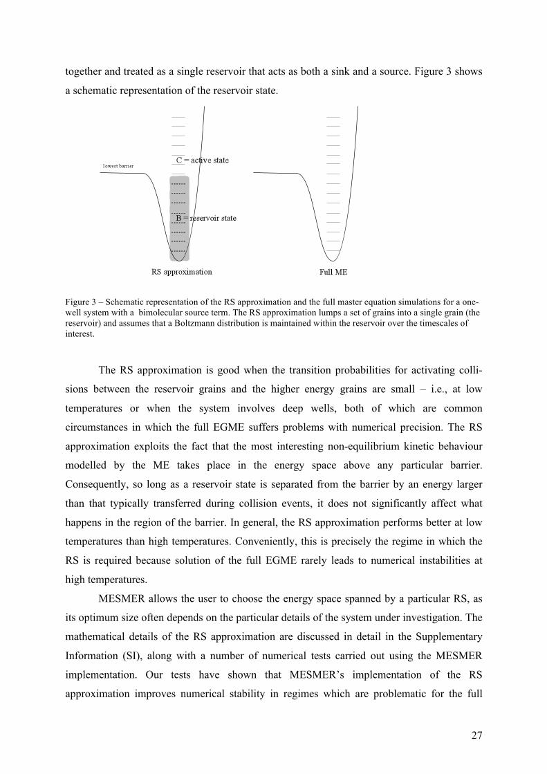
together and treated as a single reservoir that acts as both a sink and a source. Figure 3 shows

a schematic representation of the reservoir state.

Figure 3 – Schematic representation of the RS approximation and the full master equation simulations for a one-well system with a bimolecular source term. The RS approximation lumps a set of grains into a single grain (the reservoir) and assumes that a Boltzmann distribution is maintained within the reservoir over the timescales of interest.

The RS approximation is good when the transition probabilities for activating colli-

sions between the reservoir grains and the higher energy grains are small – i.e., at low

temperatures or when the system involves deep wells, both of which are common

circumstances in which the full EGME suffers problems with numerical precision. The RS

approximation exploits the fact that the most interesting non-equilibrium kinetic behaviour

modelled by the ME takes place in the energy space above any particular barrier.

Consequently, so long as a reservoir state is separated from the barrier by an energy larger

than that typically transferred during collision events, it does not significantly affect what

happens in the region of the barrier. In general, the RS approximation performs better at low

temperatures than high temperatures. Conveniently, this is precisely the regime in which the

RS is required because solution of the full EGME rarely leads to numerical instabilities at

high temperatures.

MESMER allows the user to choose the energy space spanned by a particular RS, as

its optimum size often depends on the particular details of the system under investigation. The

mathematical details of the RS approximation are discussed in detail in the Supplementary

Information (SI), along with a number of numerical tests carried out using the MESMER

implementation. Our tests have shown that MESMER’s implementation of the RS

approximation improves numerical stability in regimes which are problematic for the full

28

EGME. Where comparisons are possible, the RS method gives results in excellent agreement

with the full EGME. For some systems, the RS approximation results in computational

speedups of nearly an order of magnitude.52

3.4.3. Contracted basis method

The mathematic details of the contracted basis method are outlined in Appendix A.

The practical objective of this method is similar to that of the RS method: to accurately

represent a full EGME system using a reduced matrix and thus reduce the computational

expense of the diagonalization. This approach is closely related to that proposed by Venkatesh

and co-workers,55,56 who expressed the ME in a basis of analytic functions rather than δ-

functions; however, it differs insofar as the basis functions are derived from a grained solution

to a single well master equation. The present approach is also closely related to the

perturbation approach described by Snider57 and elements of it have been used more recently

by Miller and co-workers in their analysis of detailed balance.22 Some preliminary results for

an approximate model of the isomerisation between the primary and secondary pentyl radicals

are presented in the SI.

3.5. Collisional energy transfer models

The most common model for calculating collisional energy transition probabilities is

the so-called exponential down model, and this is what is presently implemented within

MESMER. The exponential down model, which assumes that the energy transfer probability

depends only on the internal energy of the molecule, and not on its collisional history or its

configuration, calculates collisional energy transition probabilities as:9,13,58

(38)

where , is a normalization constant, and is the average energy transferred

per collision in a downward direction. The transition probabilities for energy transfer in the

upward direction may be obtained via detailed balance. The exponential down model was

proposed on the basis of results from scattering theory,59,60 and reflects the common sense

29

notion that collisions which transfer large amounts of energy are less probable than those that

transfer small amounts of energy.9 Other models with different transition probability

distributions have been proposed, such as Gaussian models27 and double exponential

models.13 It has often been noted that classical trajectory simulations as well as experimental

data suggest that the exponential down model is perhaps not the most accurate for describing

collisional transition probabilities, and that models with longer tails are more accurate.13,58,61-

64

Nevertheless, most published EGME studies utilize the single exponential down

model.5 This is partially because other functions (e.g., double exponential models) feature

more parameters, and systematic techniques for assigning parameter values have yet to be

established. Additionally, given the extensive use of the single exponential down model in

the literature, a set of typical values has emerged. For example, at room temperature

He bath gas tends to have values from ~50-300 cm-1,26,65-70 while O2 and N2 bath gases

tend to have slightly higher values of ~250-500 cm-1.67,69,71 In general, is left as

a variable parameter determined by fitting to experimental data, within the limits given above,

and it usually shows a slight positive temperature dependence in one dimensional ME

analyses. The origin of the temperature dependence is not entirely clear, although it has been

suggested that it may relate to rotational relaxation,72 an observation which is compatible with

the fact that classical trajectory calculations have identified the dependence of on the

angular momentum of the target molecule.20 Experimentally, higher temperatures correspond

to higher angular momentum states, and in the one-dimensional ME, this may be manifest as

an effective increase in

€

ΔE d .72

3.6. Data fitting methods

As discussed above, the analysis of experimental data is often an important objective

for MESMER. For example, one might want to fit experimental data in order to obtain a

reaction threshold or high pressure Arrhenius parameters. It is generally the case that the

calculated rate coefficients have a non-linear dependence on these parameters, in which case

it is normal to optimize the merit function using an algorithm based on the Levenberg-

Marquardt approach. However, such an algorithm requires a knowledge of the derivatives of

30

the rate coefficients with respect to the parameters. The difficulty with this is that the rate

coefficients are derived from eigenvalues of the matrix M, which are calculated numerically.

In general, there is no direct analytic relationship between the rate coefficients and the

parameters on which they depend, so that analytic derivatives cannot be calculated.

This leaves the option of numerical derivatives, despite the fact that they often involve

a large computational expense with an increase in the number of fit parameters. The expense

arises because derivatives for a particular parameter requires calculation of for (at least)

two other points in parameter space, resulting in several diagonalizations of M at each

pressure and temperature point in the experimental set. Hence it is advantageous to invoke as

few diagonalizations as possible in minimizing .

MESMER offers two approaches to the optimization of : the Powell conjugate

direction method and a Levenberg-Marquardt approach based on numerical derivatives.37 The

Powell conjugate direction method requires line searches to be performed in the chosen

parameter space and these are done using golden section searches. The directions of the line

searches are initially taken as the set of mutually perpendicular unit vectors of the parameter

space, but these search directions are updated as the individual line searches are completed in

accordance with Powell’s algorithm. The Levenberg-Marquardt implementation follows a

standard pattern with the minor alteration that limits can be placed on the range of values a

parameter may take during a search. Our experience to date suggests that the Levenberg-

Marquardt algorithm, despite initial heavy costs, is the most efficient method.

4. Examples

4.1. MESMER test examples

During the implementation of MESMER, a number of tests were developed in order to

monitor the impact of code changes and provide a test suite for future developments. These

test systems are supplied with the MESMER distribution and are based on a number of

previous studies, most of which are relevant to combustion and atmospheric chemistry.

Included in these tests are:

31

(1) Simple unimolecular dissociation – i.e., the decomposition of the iso-propyl

radical to propene and a hydrogen atom, which includes the quantum mechani-

cal treatment of hindered internal rotors described above;73

(2) Isomerization reactions of the n-pentyl radical;10

(3) The reaction of the acetyl radical with excess oxygen, an example of a two-

well system. It features a source term, a tunnelling treatment, and fitting to ex-

perimental data using a minimum χ2 criterion.67 The association of CH3CO +

O2 has been shown experimentally to give OH at low pressures because of

isomerisation and subsequent dissociation of the initially formed peroxy radi-

cal. This type of chemistry, which involves so-called “formally direct” kinet-

ics, is important in reactions of peroxy radicals in combustion.74

(4) The reaction of the H radical with SO2,75 which features a bimolecular source

term and makes use of extended precision libraries for matrix diagonalization;

(5) The reaction of OH with NO, which features a bimolecular source term, and an

example of how to use MESMER to perform a so-called “thermodynamic

data” calculation. The results of this calculation give ΔH(T), ΔS(T), and ΔG(T)

for OH, NO, and HNO2 at a range of temperatures.

4.2. Atmospheric chemistry

MESMER has so far been applied to a number of chemical kinetic systems relevant to

both terrestrial and extra-planetary atmospheres, including:

(1) The pressure and temperature dependence of the reaction of OH with acetylene,

which includes a bimolecular source term and an ILT treatment of the association

process;69

(2) The atmospheric kinetic sequence that follows association between the benzene-

OH adduct and O2, which involves a bimolecular source term with multiple asso-

ciation channels;76

(3) The kinetics between O2(1Δg) + Ca, which utilizes increased precision arithmetic,

non-adiabatic spin-hopping kinetics, and ILT treatments to describe both associa-

tion and dissociation processes.77

(4) An examination of the kinetics between 1CH2 and acetylene, which implements a

reservoir state approximation and matrix diagonalization using increased numeri-

32

cal precision and three reservoir states.52,78 This reaction produces the C3H3 radi-

cal, which can act as a route to benzene and lead to subsequent haze formation in

Titan’s atmosphere.

(5) The atmospheric abstraction and addition kinetics of OH + polybrominated di-

phenyl ethers (PBDEs).79

4.3. Organic chemistry

In addition to the aforementioned examples, we have successfully applied MESMER

to understand experimentally observed kinetics and product yields in solution phase synthetic

chemistry. To our knowledge, these studies represent the first time that master equation

treatments have been extended to solution phase systems. So far, the systems we have

investigated include:

(1) The hydroboration of propene to give OH substituted Markovinikov and anti-

Markovnikov products.3 This system implements a source term and an isolated bi-

nary collision treatment of solvent-solute relaxation. The EGME quantitatively re-

produces the experimentally observed product ratios observed at different tem-

peratures, and suggests the reaction occurs in a regime where chemical reaction

timescales compete with collisional relaxation timescales.

(2) [1,5] Hydrogen migration in chemically activated cyclopentadiene.2 Again, using

an isolated binary collision treatment of solvent-solute relaxation, the EGME was

able to provide a good description of the experimentally observed hydrogen migra-

tion yield arising from a chemically activated cyclopentadienyl radical. The results

suggest that the reaction occurs in a regime where chemical reaction timescales

compete with collisional relaxation timescales.

5. Conclusions, outlook, future development

The goal of the MESMER application is to facilitate the analysis and interpretation of

kinetic rate data for systems whose potential energy surface consists of a number of stationary

points, and where system-bath energy transfer affects kinetic outcomes. In the limit of very

high pressures, MESMER gives rate coefficients which are identical to those obtained from

thermal TST, while in the limit of very low pressures, MESMER gives rate coefficients which

33

are identical to those obtained from RRKM theory. MESMER is particularly well suited to

analyzing kinetics in intermediate pressure regimes, where a great deal of chemistry in nature

occurs. Alongside increasingly accurate thermodynamics data, continuing developments in

electronic structure theory, improved fundamental understanding of energy transfer within gas

and condensed phases, and expanding databases of reliable experimental data, we envision

that tools like MESMER will eventually enable reliable and routine prediction of non-

equilibrium kinetics in arbitrary systems.

With this vision in mind, MESMER has been built to provide a user-friendly, open-

source, object oriented framework with a number of key design principles that we hope will

facilitate open-source development: (1) the MESMER object model allows the natural

definition (and extension) of molecular species and the reactions in which they participate,

and this is reflected in MESMER’s flexible, XML based, I/O facility; (2) through the device

of plugin classes, it should be relatively straightforward for a number of workers to extend the

code and contribute to the development of MESMER, and (3) MESMER includes the

provision of facilities to analyse and fit data, which will enable us to construct a database for

analysis and fitting.

The development of MESMER is ongoing and potential future work includes:

• The development of a graphical user interface (GUI). While the use of an XML based

data format is key to the interoperability of MESMER with other applications, and there

are a number of XML editors available, the input of data would be greatly assisted by a

user interface that supported the MESMER data specification.

• A wide range of databases are available that contain information pertinent to a

MEMSER calculation, e.g. thermochemical and ab initio properties databases such as

those made available by NIST, or through active thermochemical tables.80 It would be of

enormous benefit to the research community if a means of interfacing these databases with

MESMER could be established.

• Central to almost all MESMER calculations is the diagonalization of a matrix, and the

performance of MESMER depends on the efficiency of this diagonalization. In the case of

data fitting, diagonalization must be performed a large number of times for different

conditions and parameter values. This permits an “embarrassingly parallel” implementa-

tion of MESMER built on libraries such as MPI or openMP. In addition, we are carrying

our further investigation of efficient mathematical formulations tailored to the specifics of

the problem at hand (e.g. basis contraction and reservoir states).

34

• Once a reaction system has been analysed, reporting a set of rate coefficients and/or

eigenvalues at specific temperatures and pressures is usually not the most convenient form

for use in macroscopic models. Hence we are exploring methods to efficiently represent

output data in more useful forms.

• Our recent work in applying EGME approaches to solution phase organic chemistry

opens up the possibility of extending MESMER to treat the chemistry that occurs in a

range of condensed phase and interfacial systems. These will likely require research and

development of more accurate energy transfer models that go beyond the simple

exponential down model.

Acknowledgements

This work was made possible through the help of several people not included as authors, in

particular Robin Shannon, Dr. Mark Blitz, Dr. Nicholas Green, Dr. Kevin Hughes, Dr. David

Waller, and Professor Paul Seakins. Much of the MESMER development was carried out

under the auspices of grants from the EPSRC and NERC.

35

References 1. Truhlar, D. G.; Garrett, B. C.; Klippenstein, S. J. J Phys Chem 1996, 100(31), 12771-12800. 2. Goldman, L. M.; Glowacki, D. R.; Carpenter, B. K. J Am Chem Soc 2011, 133(14), 5312-5318. 3. Glowacki, D. R.; Liang, C. H.; Marsden, S. P.; Harvey, J. N.; Pilling, M. J. J Am Chem Soc 2010, 132(39), 13621-13623. 4. Allen, J. W.; Goldsmith, C. F.; Green, W. H. PCCP Phys Chem Chem Phys 2012, 14(3), 1131-1155. 5. Golden, D. M.; Barker, J. R. Combust Flame 2011, 158(4), 602-617. 6. Barker, J. R.; Golden, D. M. Chemical Reviews (Washington, DC, United States) 2003, 103(12), 4577-4591. 7. Glowacki, D. R.; Pilling, M. J. ChemPhysChem 2010, 11(18), 3836-3843. 8. Holbrook, K. A.; Pilling, M. J.; Robertson, S. H. Unimolecular Reactions; John Wiley & Sons: Chichester, 1996. 9. Pilling, M. J.; Robertson, S. H. Annu Rev Phys Chem 2003, 54, 245-275. 10. Robertson, S. H.; Pilling, M. J.; Jitariu, L. C.; Hillier, I. H. Phys Chem Chem Phys 2007, 9(31), 4085-4097. 11. Miller, J. A.; Pilling, M. J.; Troe, J. Proc Combust Inst 2005, 30(Pt. 1), 43-88. 12. Miller, J. A.; Klippenstein, S. J.; Raffy, C. J Phys Chem A 2002, 106(19), 4904-4913. 13. Miller, J. A.; Klippenstein, S. J. J Phys Chem A 2006, 110(36), 10528-10544. 14. Klippenstein, S. J.; Miller, J. A. J Phys Chem A 2002, 106(40), 9267-9277. 15. Miller, J. A.; Klippenstein, S. J. J Phys Chem A 2003, 107(15), 2680-2692. 16. Gillespie, D. T. In Annu Rev Phys Chem; Annual Reviews: Palo Alto, 2007, p 35-55. 17. Barker, J. R. Int J Chem Kinet 2001, 33(4), 232-245. 18. Robertson, S. H.; Pilling, M. J.; Gates, K. E.; Smith, S. C. J Comput Chem 1997, 18(8), 1004-1010. 19. Green, N. J. B.; Bhatti, Z. A. PCCP 2007, 9(31), 4275-4290. 20. Barker, J. R.; Weston, R. E. J Phys Chem A 2010, 114(39), 10619-10633. 21. Smith, S. C.; Gilbert, R. G. Int J Chem Kinet 1988, 20(4), 307-329. 22. Miller, J. A.; Klippenstein, S. J.; Robertson, S. H.; Pilling, M. J.; Green, N. J. B. PCCP Phys Chem Chem Phys 2009, 11(8), 1128-1137. 23. Vereecken, L.; Huyberechts, G.; Peeters, J. Journal of Chemical Physics 1997, 106(16), 6564-6573. 24. Frankcombe, T. J.; Smith, S. C. J Theor Comput Chem 2003, 2(2), 179-191. 25. Frankcombe, T. J.; Smith, S. C. Theor Chem Acc 2009, 124(5-6), 303-317. 26. Gannon, K. L.; Glowacki, D. R.; Blitz, M. A.; Hughes, K. J.; Pilling, M. J.; Seakins, P. W. J Phys Chem A 2007, 111(29), 6679-6692. 27. Gilbert, R. G.; Smith, S. C. Theory of Unimolecular and Recombination Reactions; Blackwell Scientific Publications: Oxford, 1990. 28. Gang, J.; Pilling, M. J.; Robertson, S. H. Chem Phys 1998, 231(2-3), 183-192. 29. Fernandez-Ramos, A.; Ellingson, B. A.; Meana-Paneda, R.; Marques, J. M. C.; Truhlar, D. G. Theor Chem Acc 2007, 118(4), 813-826. 30. King, G. W.; Hainer, R. M.; Cross, P. C. Journal of Chemical Physics 1943, 11(1), 27-42. 31. Hougen, J. T. NBS Monograph 1970, 115. 32. Chuang, Y. Y.; Truhlar, D. G. Journal of Chemical Physics 2000, 112(3), 1221-1228. 33. Nielsen, H. H. Phys Rev 1932, 40(3), 0445-0456.

36

34. Barker, J. R.; Shovlin, C. N. Chemical Physics Letters 2004, 383(1-2), 203-207. 35. Lewis, J. D.; Malloy, T. B.; Chao, T. H.; Laane, J. J Mol Struct 1972, 12(3), 427-&. 36. Abramowitz, M.; Stegun, I. A. Handbook of Mathematical Functions: New York, 1972. 37. Press, W. H.; Teukolsky, S. A.; Vetterling, W. T.; Flannery, B. P. Numerical Recipes in C++; Cambridge University Press: Cambridge, 2002. 38. Accelyrs-Software. San Diego, CA, 2011. 39. Lourderaj, U.; Hase, W. L. J Phys Chem A 2009, 113(11), 2236-2253. 40. Baer, T.; Hase, W. L. Unimolecular reaction dynamics: theory and experiments; Oxford University Press: New York, 1996. 41. Klippenstein, S. J.; Green, N. J. B. In Comprehensive Chemical Kinetics; Elsevier, 2003, p 55-103. 42. Georgievskii, Y.; Klippenstein, S. J. Journal of Chemical Physics 2003, 118(12), 5442-5455. 43. Georgievskii, Y.; Klippenstein, S. J. J Phys Chem A 2003, 107(46), 9776-9781. 44. Davies, J. W.; Green, N. J. B.; Pilling, M. J. Chemical Physics Letters 1986, 126(3-4), 373-379. 45. Miller, W. H. J Am Chem Soc 1979, 101(23), 6810-6814. 46. Harvey, J. N. PCCP Phys Chem Chem Phys 2007, 9(3), 331-343. 47. Jasper, A. W.; Zhu, C. Y.; Nangia, S.; Truhlar, D. G. Faraday Discuss 2004, 127, 1-22. 48. Nikitin, E. E. Annu Rev Phys Chem 1999, 50, 1-21. 49. Harvey, J. N.; Aschi, M. Faraday Discuss 2003, 124, 129-143. 50. Delos, J. B.; Thorson, W. R. Physical Review A 1972, 6(2), 728-&. 51. Bartis, J. T.; Widom, B. Journal of Chemical Physics 1974, 60(9), 3474-3482. 52. Gannon, K. L.; Blitz, M. A.; Liang, C. H.; Pilling, M. J.; Seakins, P. W.; Glowacki, D. R. J Phys Chem A 2010, 114(35), 9413-9424. 53. Hida, Y.; Li, X. S.; Bailey, D. H. Arithmetic 2000, 15. 54. Schranz, H. W.; Nordholm, S. Chem Phys 1983, 74(3), 365-381. 55. Venkatesh, P. K.; Dean, A. M.; Cohen, M. H.; Carr, R. W. Journal of Chemical Physics 1999, 111(18), 8313-8329. 56. Venkatesh, P. K.; Dean, A. M.; Cohen, M. H.; Carr, R. W. Journal of Chemical Physics 1997, 107(21), 8904-8916. 57. Snider, N. S. Journal of Chemical Physics 1965, 42(2), 548-&. 58. Barker, J. R. Int J Chem Kinet 2009, 41(12), 748-763. 59. Jackson, J. M.; Mott, N. F. Proc R soc Lond Ser A-Contain Pap Math Phys Character 1932, 137(833), 703-717. 60. Penner, A. P.; Forst, W. Journal of Chemical Physics 1977, 67(11), 5296-5307. 61. Lenzer, T.; Luther, K.; Reihs, K.; Symonds, A. C. Journal of Chemical Physics 2000, 112(9), 4090-4110. 62. Hold, U.; Lenzer, T.; Luther, K.; Reihs, K.; Symonds, A. C. Journal of Chemical Physics 2000, 112(9), 4076-4089. 63. Hold, U.; Lenzer, T.; Luther, K.; Symonds, A. C. Journal of Chemical Physics 2003, 119(21), 11192-11211. 64. Jasper, A. W.; Miller, J. A. J Phys Chem A 2011, 115(24), 6438-6455. 65. Golden, D. M.; Barker, J. R.; Lohr, L. L. J Phys Chem A 2003, 107(50), 11057-11071. 66. Miller, J. A.; Senosiain, J. P.; Klippenstein, S. J.; Georgievskii, Y. J Phys Chem A 2008, 112(39), 9429-9438. 67. Carr, S. A.; Glowacki, D. R.; Liang, C. H.; Baeza-Romero, M. T.; Blitz, M. A.; Pilling, M. J.; Seakins, P. W. J Phys Chem A 2011, 115(6), 1069-1085.

37

68. Zador, J.; Klippenstein, S. J.; Miller, J. A. J Phys Chem A 2011, 115(36), 10218-10225. 69. McKee, K. W.; Blitz, M. A.; Cleary, P. A.; Glowacki, D. R.; Pilling, M. J.; Seakins, P. W.; Wang, L. J Phys Chem A 2007, 111(19), 4043-4055. 70. Goldsmith, C. F.; Green, W. H.; Klippenstein, S. J. J Phys Chem A 2012, 116(13), 3325-3346. 71. Goldsmith, C. F.; Klippenstein, S. J.; Green, W. H. Proceedings of the Combustion Institute 2011, 33, 273-282. 72. Miller, J. A. Faraday Discuss 2001, 119(Combustion Chemistry: Elementary Reactions to Macroscopic Processes), 461-475. 73. Seakins, P. W.; Robertson, S. H.; Pilling, M. J.; Slagle, I. R.; Gmurczyk, G. W.; Bencsura, A.; Gutman, D.; Tsang, W. J Phys Chem 1993, 97(17), 4450-4458. 74. Clifford, E. P.; Farrell, J. T.; DeSain, J. D.; Taatjes, C. A. J Phys Chem A 2000, 104(49), 11549-11560. 75. Blitz, M. A.; Hughes, K. J.; Pilling, M. J.; Robertson, S. H. J Phys Chem A 2006, 110(9), 2996-3009. 76. Glowacki, D. R.; Wang, L. M.; Pilling, M. J. J Phys Chem A 2009, 113(18), 5385-5396. 77. Plane, J. M. C.; Whalley, C. L.; Soriano, L.; Goddard, A.; Harvey, J. N.; Glowacki, D. R.; Viggiano, A. A. Journal of Chemical Physics in press. 78. Gannon, K. L.; Blitz, M. A.; Liang, C. H.; Pilling, M. J.; Seakins, P. W.; Glowacki, D. R.; Harvey, J. N. Faraday Discuss 2010, 147, 173-188. 79. Zhou, J.; Chen, J. W.; Liang, C. H.; Xie, Q.; Wang, Y. N.; Zhang, S. Y.; Qiao, X. L.; Li, X. H. Environ Sci Technol 2011, 45(11), 4839-4845. 80. Ruscic, B.; Pinzon, R. E.; Morton, M. L.; Srinivasan, N. K.; Su, M. C.; Sutherland, J. W.; Michael, J. V. J Phys Chem A 2006, 110(21), 6592-6601. 81. Szabo, A.; Ostlund, N. S. Modern Quantum Chemistry; Dover: New York, 1996. 82. Bramley, M. J.; Handy, N. C. Journal of Chemical Physics 1993, 98(2), 1378-1397.

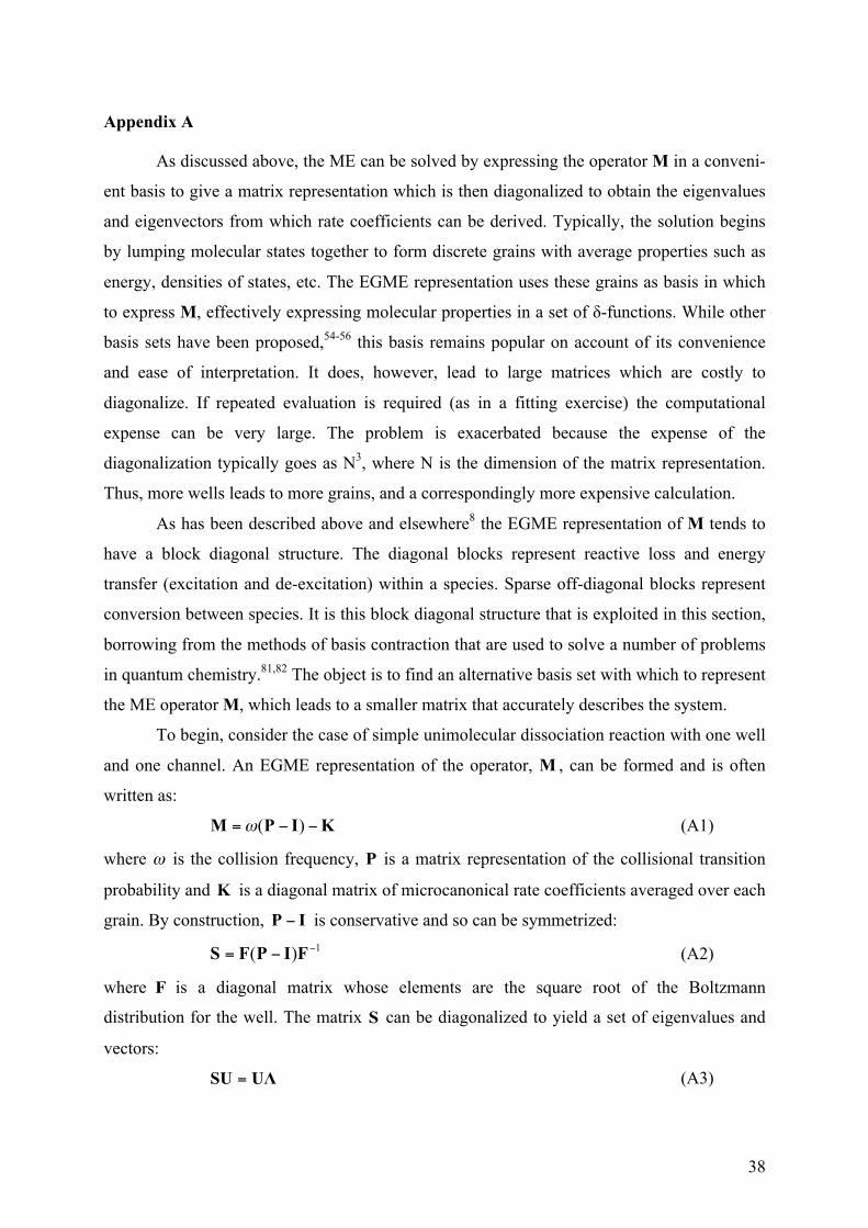
38

Appendix A

As discussed above, the ME can be solved by expressing the operator M in a conveni-

ent basis to give a matrix representation which is then diagonalized to obtain the eigenvalues

and eigenvectors from which rate coefficients can be derived. Typically, the solution begins

by lumping molecular states together to form discrete grains with average properties such as

energy, densities of states, etc. The EGME representation uses these grains as basis in which

to express M, effectively expressing molecular properties in a set of δ-functions. While other

basis sets have been proposed,54-56 this basis remains popular on account of its convenience

and ease of interpretation. It does, however, lead to large matrices which are costly to

diagonalize. If repeated evaluation is required (as in a fitting exercise) the computational

expense can be very large. The problem is exacerbated because the expense of the

diagonalization typically goes as N3, where N is the dimension of the matrix representation.

Thus, more wells leads to more grains, and a correspondingly more expensive calculation.

As has been described above and elsewhere8 the EGME representation of M tends to

have a block diagonal structure. The diagonal blocks represent reactive loss and energy

transfer (excitation and de-excitation) within a species. Sparse off-diagonal blocks represent

conversion between species. It is this block diagonal structure that is exploited in this section,

borrowing from the methods of basis contraction that are used to solve a number of problems

in quantum chemistry.81,82 The object is to find an alternative basis set with which to represent

the ME operator M, which leads to a smaller matrix that accurately describes the system.

To begin, consider the case of simple unimolecular dissociation reaction with one well

and one channel. An EGME representation of the operator, , can be formed and is often

written as:

(A1)

where is the collision frequency, is a matrix representation of the collisional transition

probability and is a diagonal matrix of microcanonical rate coefficients averaged over each

grain. By construction, is conservative and so can be symmetrized:

(A2)

where is a diagonal matrix whose elements are the square root of the Boltzmann

distribution for the well. The matrix can be diagonalized to yield a set of eigenvalues and

vectors:

(A3)

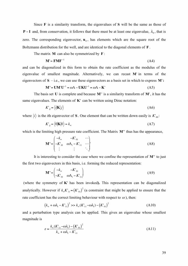
39

Since is a similarity transform, the eigenvalues of will be the same as those of

and, from conservation, it follows that there must be at least one eigenvalue, , that is

zero. The corresponding eigenvector, , has elements which are the square root of the

Boltzmann distribution for the well, and are identical to the diagonal elements of .

The matrix can also be symmetrized by :

(A4)

and can be diagonalized in this form to obtain the rate coefficient as the modulus of the

eigenvalue of smallest magnitude. Alternatively, we can recast in terms of the

eigenvectors of – i.e., we can use these eigenvectors as a basis set in which to express :

€

M' '=UM'U−1 =ωΛ −UKU−1 =ωΛ −K ' (A5)

The basis set

€

U is complete and because

€

M' ' is a similarity transform of , it has the

same eigenvalues. The elements of can be written using Dirac notation:

€

K 'ij = iK j (A6)

where is the ith eigenvector of . One element that can be written down easily is

€

K '00 :

€

K 'ij = 0K 0 = k∞ (A7)

which is the limiting high pressure rate coefficient. The Matrix thus has the appearance,

€

M' '=−k∞ −K '01

−K '10 ωΛ1 −K '11

' (A8)

It is interesting to consider the case where we confine the representation of to just

the first two eigenvectors in this basis, i.e. forming the reduced representation:

€

M' '=−k∞ −K '01−K '01 ωΛ1 −K '11

(A9)

(where the symmetry of has been invoked). This representation can be diagonalized

analytically. However if

€

k∞K '11 ≈ K '01( )2 (a constraint that might be applied to ensure that the

rate coefficient has the correct limiting behaviour with respect to ), then:

€

k∞ +ωλ1 −K '11( )2 >> k∞(K '11−ωλ1) − K '01( )2 (A10)

and a perturbation type analysis can be applied. This gives an eigenvalue whose smallest

magnitude is

€

ε ≈k∞(K '11−ωλ1) − K '01( )2

k∞ +ωλ1 −K '11 (A11)

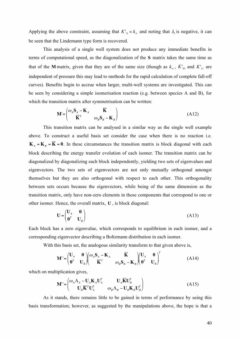
40

Applying the above constraint, assuming that and noting that is negative, it can

be seen that the Lindemann type form is recovered.

This analysis of a single well system does not produce any immediate benefits in

terms of computational speed, as the diagonalization of the matrix takes the same time as

that of the matrix, given that they are of the same size (though as , and are

independent of pressure this may lead to methods for the rapid calculation of complete fall-off

curves). Benefits begin to accrue when larger, multi-well systems are investigated. This can

be seen by considering a simple isomerisation reaction (e.g. between species A and B), for

which the transition matrix after symmetrisation can be written:

€

M'=ωASA −KA K

K T ωBSB −KB

(A12)

This transition matrix can be analysed in a similar way as the single well example

above. To construct a useful basis set consider the case when there is no reaction i.e.

€

KA = KB = K = 0. In these circumstances the transition matrix is block diagonal with each

block describing the energy transfer evolution of each isomer. The transition matrix can be

diagonalized by diagonalizing each block independently, yielding two sets of eigenvalues and

eigenvectors. The two sets of eigenvectors are not only mutually orthogonal amongst

themselves but they are also orthogonal with respect to each other. This orthogonality

between sets occurs because the eigenvectors, while being of the same dimension as the

transition matrix, only have non-zero elements in those components that correspond to one or

other isomer. Hence, the overall matrix, , is block diagonal:

€

U =UA 00T UB

(A13)

Each block has a zero eigenvalue, which corresponds to equilibrium in each isomer, and a

corresponding eigenvector describing a Boltzmann distribution in each isomer.

With this basis set, the analogous similarity transform to that given above is,

€

M' '=UA 00T UB

ωASA −KA K

K T ωBSB −KB

UA 00T UB

T

(A14)

which on multiplication gives,

€

M' '=ωAΛA −UAKAUA

T UAK UBT

UBK TUAT ωBΛB −UBKBUB

T

(A15)

As it stands, there remains little to be gained in terms of performance by using this

basis transformation; however, as suggested by the manipulations above, the hope is that a

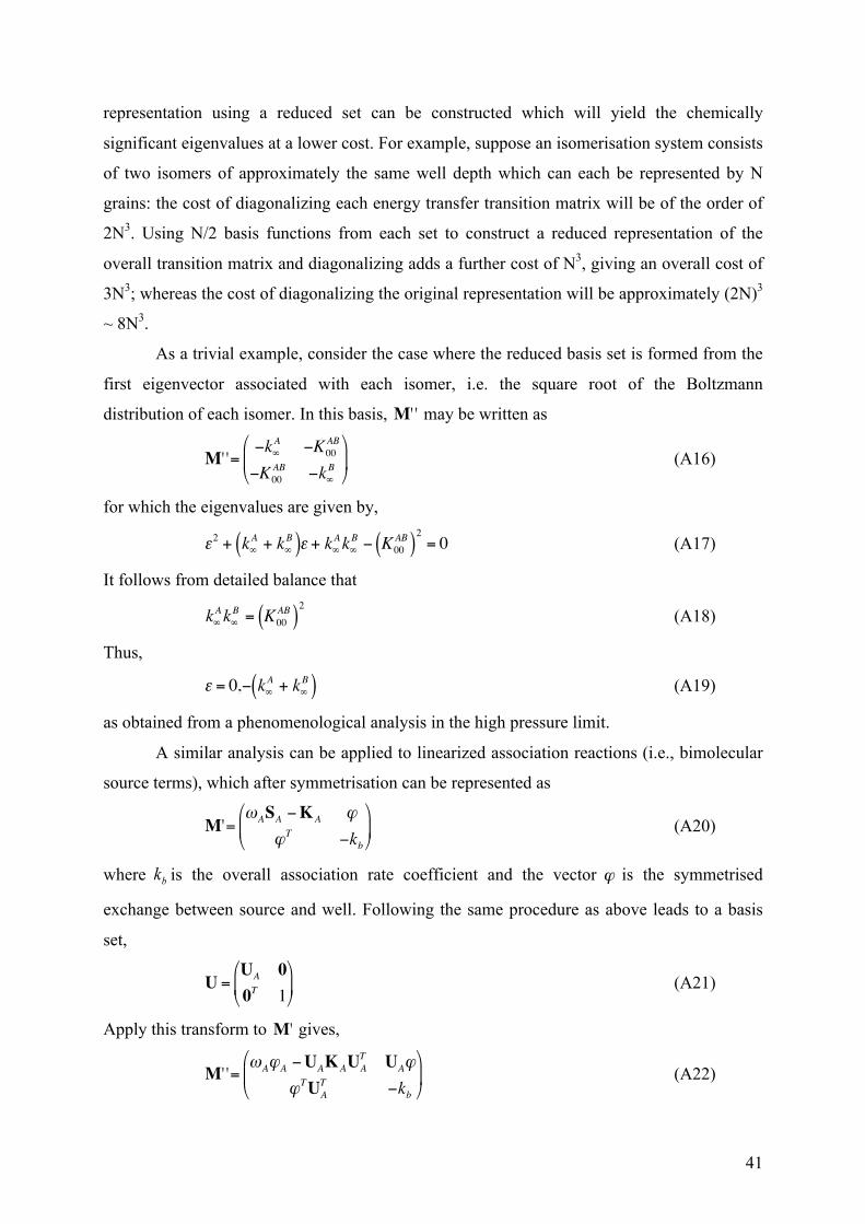
41

representation using a reduced set can be constructed which will yield the chemically

significant eigenvalues at a lower cost. For example, suppose an isomerisation system consists

of two isomers of approximately the same well depth which can each be represented by N

grains: the cost of diagonalizing each energy transfer transition matrix will be of the order of

2N3. Using N/2 basis functions from each set to construct a reduced representation of the

overall transition matrix and diagonalizing adds a further cost of N3, giving an overall cost of

3N3; whereas the cost of diagonalizing the original representation will be approximately (2N)3

~ 8N3.

As a trivial example, consider the case where the reduced basis set is formed from the

first eigenvector associated with each isomer, i.e. the square root of the Boltzmann

distribution of each isomer. In this basis,

€

M' ' may be written as

€

M' '=−k∞

A −K00AB

−K00AB −k∞

B

(A16)

for which the eigenvalues are given by,

€

ε2 + k∞A + k∞

B( )ε + k∞Ak∞

B − K00AB( )

2= 0 (A17)

It follows from detailed balance that

€

k∞Ak∞

B = K00AB( )

2 (A18)

Thus,

€

ε = 0,− k∞A + k∞

B( ) (A19)

as obtained from a phenomenological analysis in the high pressure limit.

A similar analysis can be applied to linearized association reactions (i.e., bimolecular

source terms), which after symmetrisation can be represented as

€

M'=ωASA −KA ϕ

ϕT −kb

(A20)

where is the overall association rate coefficient and the vector

€

ϕ is the symmetrised

exchange between source and well. Following the same procedure as above leads to a basis

set,

€

U =UA 00T 1

(A21)

Apply this transform to

€

M' gives,

€

M' '=ωAϕA −UAKAUA

T UAϕ

ϕTUAT −kb

(A22)

42

The reduced basis set approach outlined in this appendix has been implemented in

MESMER and an initial assessment made by modelling a simple isomerisation system based

on the inter-conversion of primary and secondary pentyl radicals. Results and timings are

discussed in the supplementary information. We expect that the basis set contraction method

may have uses in extended precision calculations as well as in so-called “two dimensional ME

models”, which account for angular momentum conservation. These 2d master equation

treatments generally result in very large matrices, and contraction schemes may offer a useful

size reduction.

43

Supplementary Information

MESMER: An open-source Master Equation Solver for Multi-Energy well Reactions

David R. Glowacki, Chi-Hsiu Liang, Christopher Morley, Michael J. Pilling, and Struan H. Robertson

Contracted basis set approach

The contracted basis set approach outlined in the associated paper has been tested by

modelling a simple isomerisation system based on the inter-conversion of primary and

secondary pentyl radicals, which has been described previously.1 External rotors were treated

classically and all internal modes where treated as harmonic oscillators. Bath gas parameters

for Argon were used to define the collision frequency. A grain size of 100 cm-1 was used and

the maximum energy was set as 24300 cm-1. Two types of calculation where run: a full ME

calculation using the standard δ–function basis set, which gave an overall matrix size of 561,

and a contracted basis set calculation using a basis derived from the first 100 eigenvectors of

each isomer, giving an overall matrix of dimension 200. For this system there are two

chemically significant eigenvalues, one of which is zero and is associated with the

equilibrium distribution.

Table 1 shows the value of the second chemically significant eigenvalue (the value

responsible for determining the relaxation of the system on chemically significant time scales)

for temperatures of 600 K and 1000 K and a range of bath gas concentrations. As can be seen,

agreement between the two methods is best at high concentrations, and tends to degrade as the

concentration decreases, with the situation being worse at lower temperatures. This is not

entirely surprising because the contracted basis has a bias toward the equilibrium distribution

and more basis functions may be required for lower pressures. Further investigation of this

point is in progress. On a standard desktop machine running windows 7, the calculation takes

20 s using a δ-function basis set, and 13 s using a contracted basis set.

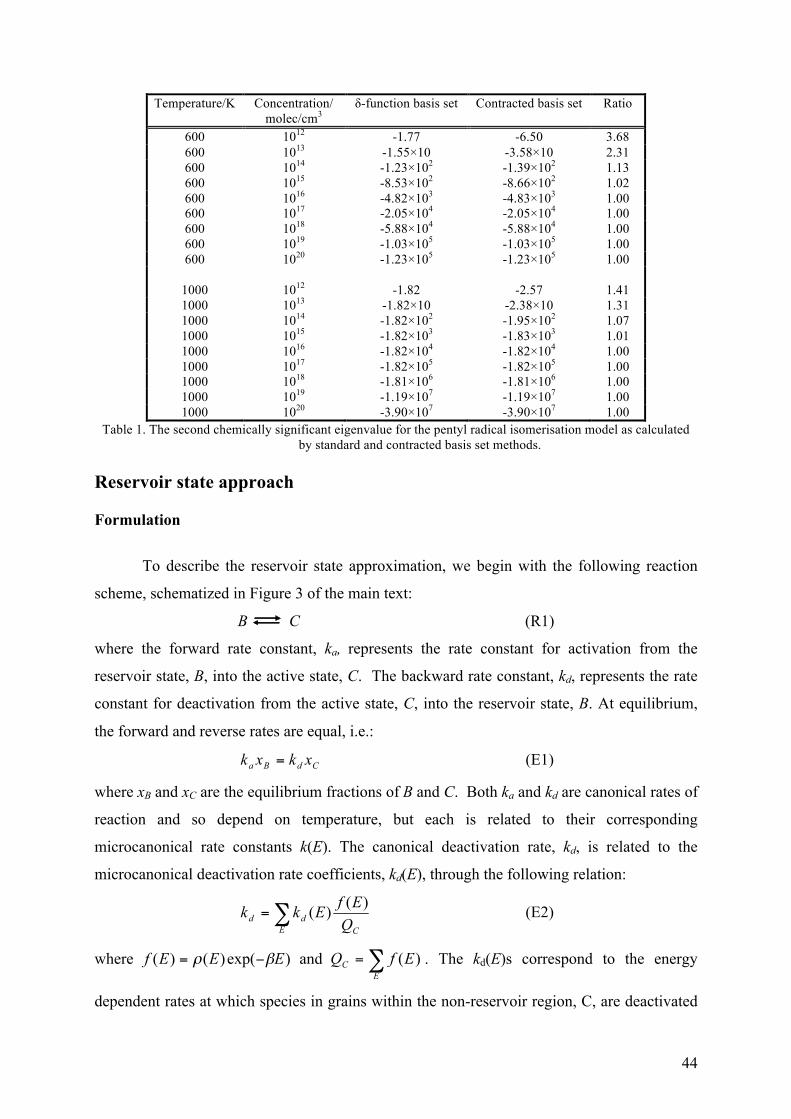
44

Temperature/K Concentration/ molec/cm3

δ-function basis set Contracted basis set Ratio

600 1012 -1.77 -6.50 3.68 600 1013 -1.55×10 -3.58×10 2.31 600 1014 -1.23×102 -1.39×102 1.13 600 1015 -8.53×102 -8.66×102 1.02 600 1016 -4.82×103 -4.83×103 1.00 600 1017 -2.05×104 -2.05×104 1.00 600 1018 -5.88×104 -5.88×104 1.00 600 1019 -1.03×105 -1.03×105 1.00 600 1020 -1.23×105 -1.23×105 1.00

1000 1012 -1.82 -2.57 1.41 1000 1013 -1.82×10 -2.38×10 1.31 1000 1014 -1.82×102 -1.95×102 1.07 1000 1015 -1.82×103 -1.83×103 1.01 1000 1016 -1.82×104 -1.82×104 1.00 1000 1017 -1.82×105 -1.82×105 1.00 1000 1018 -1.81×106 -1.81×106 1.00 1000 1019 -1.19×107 -1.19×107 1.00 1000 1020 -3.90×107 -3.90×107 1.00

Table 1. The second chemically significant eigenvalue for the pentyl radical isomerisation model as calculated by standard and contracted basis set methods.

Reservoir state approach Formulation

To describe the reservoir state approximation, we begin with the following reaction

scheme, schematized in Figure 3 of the main text:

B C (R1)

where the forward rate constant, ka, represents the rate constant for activation from the

reservoir state, B, into the active state, C. The backward rate constant, kd, represents the rate

constant for deactivation from the active state, C, into the reservoir state, B. At equilibrium,

the forward and reverse rates are equal, i.e.:

(E1)

where xB and xC are the equilibrium fractions of B and C. Both ka and kd are canonical rates of

reaction and so depend on temperature, but each is related to their corresponding

microcanonical rate constants k(E). The canonical deactivation rate, kd, is related to the

microcanonical deactivation rate coefficients, kd(E), through the following relation:

(E2)

where and . The kd(E)s correspond to the energy

dependent rates at which species in grains within the non-reservoir region, C, are deactivated

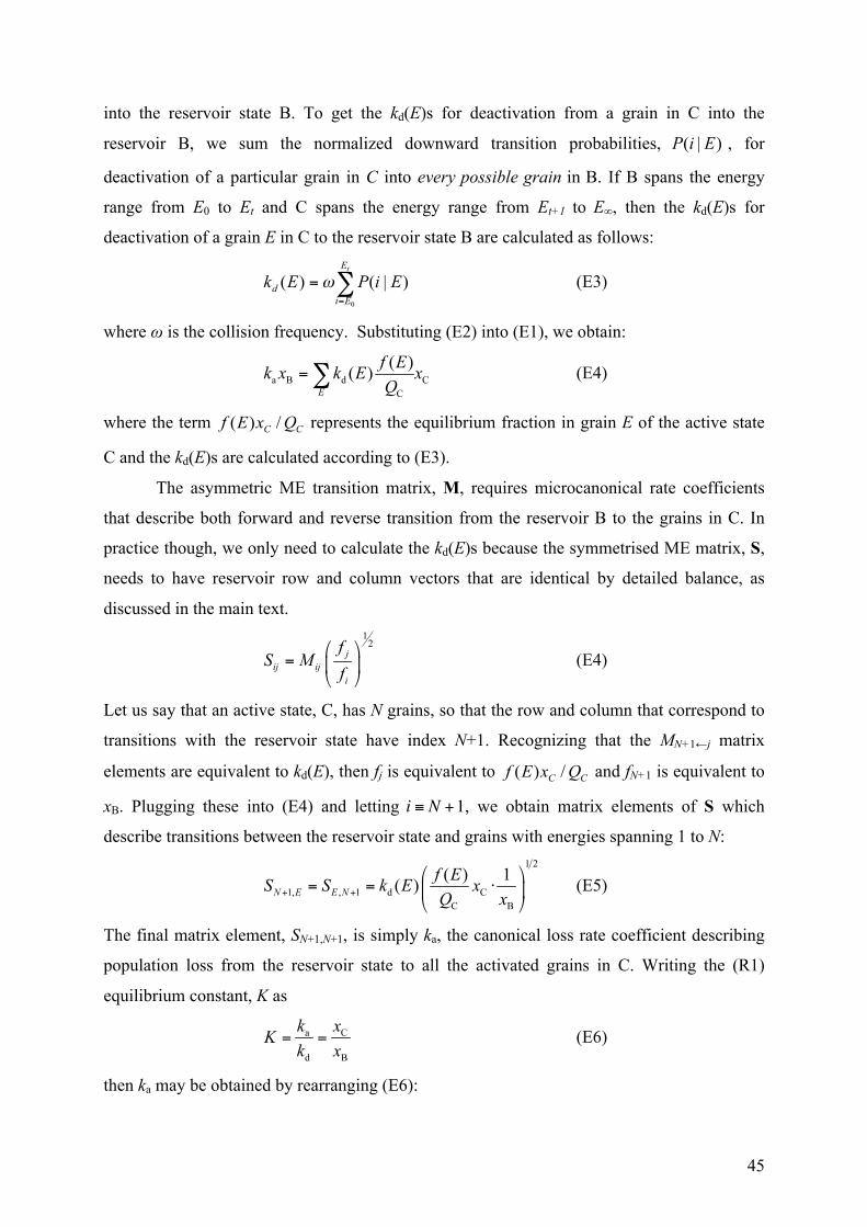
45

into the reservoir state B. To get the kd(E)s for deactivation from a grain in C into the

reservoir B, we sum the normalized downward transition probabilities, , for

deactivation of a particular grain in C into every possible grain in B. If B spans the energy

range from E0 to Et and C spans the energy range from Et+1 to E∞, then the kd(E)s for

deactivation of a grain E in C to the reservoir state B are calculated as follows:

(E3)

where ω is the collision frequency. Substituting (E2) into (E1), we obtain:

(E4)

where the term represents the equilibrium fraction in grain E of the active state

C and the kd(E)s are calculated according to (E3).

The asymmetric ME transition matrix, M, requires microcanonical rate coefficients

that describe both forward and reverse transition from the reservoir B to the grains in C. In

practice though, we only need to calculate the kd(E)s because the symmetrised ME matrix, S,

needs to have reservoir row and column vectors that are identical by detailed balance, as

discussed in the main text.

(E4)

Let us say that an active state, C, has N grains, so that the row and column that correspond to

transitions with the reservoir state have index N+1. Recognizing that the MN+1←j matrix

elements are equivalent to kd(E), then fj is equivalent to and fN+1 is equivalent to

xB. Plugging these into (E4) and letting

€

i ≡ N +1, we obtain matrix elements of S which

describe transitions between the reservoir state and grains with energies spanning 1 to N:

(E5)

The final matrix element, SN+1,N+1, is simply ka, the canonical loss rate coefficient describing

population loss from the reservoir state to all the activated grains in C. Writing the (R1)

equilibrium constant, K as

(E6)

then ka may be obtained by rearranging (E6):

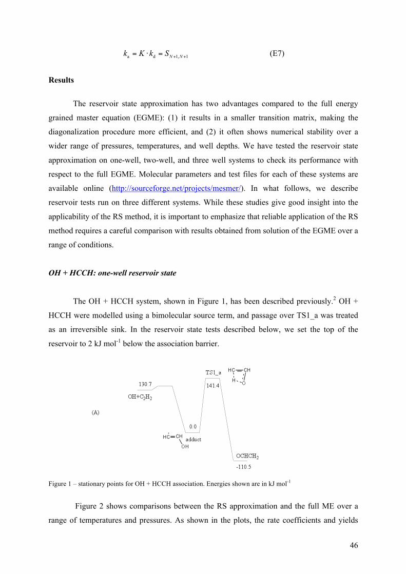
46

(E7)

Results

The reservoir state approximation has two advantages compared to the full energy

grained master equation (EGME): (1) it results in a smaller transition matrix, making the

diagonalization procedure more efficient, and (2) it often shows numerical stability over a

wider range of pressures, temperatures, and well depths. We have tested the reservoir state

approximation on one-well, two-well, and three well systems to check its performance with

respect to the full EGME. Molecular parameters and test files for each of these systems are

available online (http://sourceforge.net/projects/mesmer/). In what follows, we describe

reservoir tests run on three different systems. While these studies give good insight into the

applicability of the RS method, it is important to emphasize that reliable application of the RS

method requires a careful comparison with results obtained from solution of the EGME over a

range of conditions.

OH + HCCH: one-well reservoir state

The OH + HCCH system, shown in Figure 1, has been described previously.2 OH +

HCCH were modelled using a bimolecular source term, and passage over TS1_a was treated

as an irreversible sink. In the reservoir state tests described below, we set the top of the

reservoir to 2 kJ mol-1 below the association barrier.

Figure 1 – stationary points for OH + HCCH association. Energies shown are in kJ mol-1

Figure 2 shows comparisons between the RS approximation and the full ME over a

range of temperatures and pressures. As shown in the plots, the rate coefficients and yields

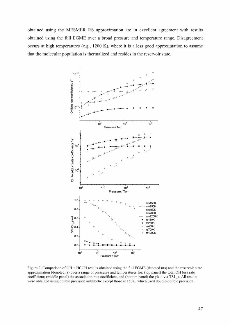
47

obtained using the MESMER RS approximation are in excellent agreement with results

obtained using the full EGME over a broad pressure and temperature range. Disagreement

occurs at high temperatures (e.g., 1200 K), where it is a less good approximation to assume

that the molecular population is thermalized and resides in the reservoir state.

Figure 2: Comparison of OH + HCCH results obtained using the full EGME (denoted nrs) and the reservoir state approximation (denoted rs) over a range of pressures and temperatures for: (top panel) the total OH loss rate coefficient; (middle panel) the association rate coefficient, and (bottom panel) the yield via TS1_a. All results were obtained using double precision arithmetic except those at 150K, which used double-double precision.

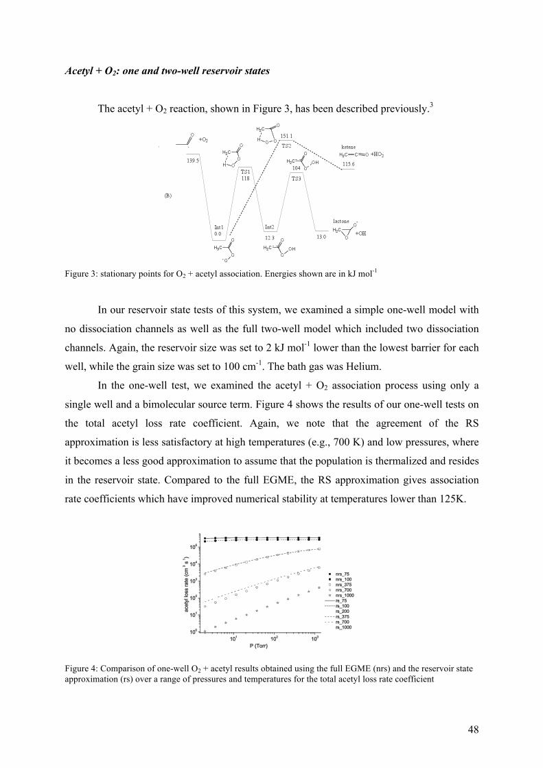
48

Acetyl + O2: one and two-well reservoir states

The acetyl + O2 reaction, shown in Figure 3, has been described previously.3

Figure 3: stationary points for O2 + acetyl association. Energies shown are in kJ mol-1

In our reservoir state tests of this system, we examined a simple one-well model with

no dissociation channels as well as the full two-well model which included two dissociation

channels. Again, the reservoir size was set to 2 kJ mol-1 lower than the lowest barrier for each

well, while the grain size was set to 100 cm-1. The bath gas was Helium.

In the one-well test, we examined the acetyl + O2 association process using only a

single well and a bimolecular source term. Figure 4 shows the results of our one-well tests on

the total acetyl loss rate coefficient. Again, we note that the agreement of the RS

approximation is less satisfactory at high temperatures (e.g., 700 K) and low pressures, where

it becomes a less good approximation to assume that the population is thermalized and resides

in the reservoir state. Compared to the full EGME, the RS approximation gives association

rate coefficients which have improved numerical stability at temperatures lower than 125K.

Figure 4: Comparison of one-well O2 + acetyl results obtained using the full EGME (nrs) and the reservoir state approximation (rs) over a range of pressures and temperatures for the total acetyl loss rate coefficient

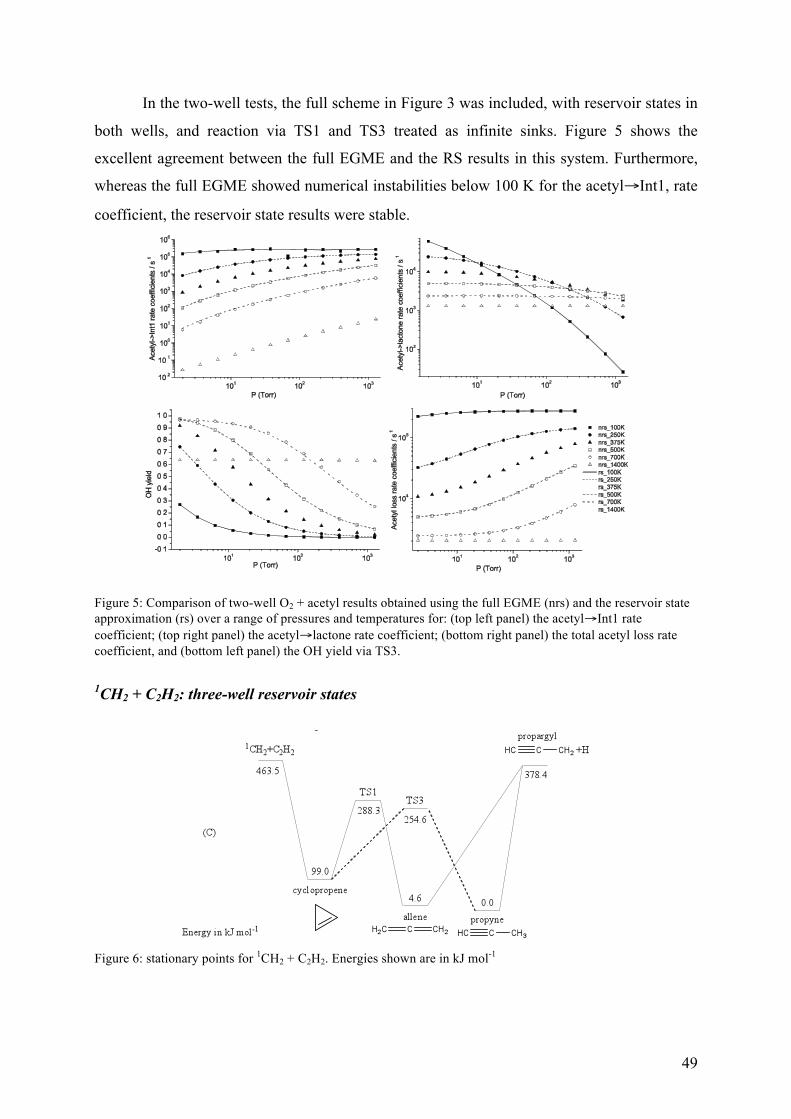
49

In the two-well tests, the full scheme in Figure 3 was included, with reservoir states in

both wells, and reaction via TS1 and TS3 treated as infinite sinks. Figure 5 shows the

excellent agreement between the full EGME and the RS results in this system. Furthermore,

whereas the full EGME showed numerical instabilities below 100 K for the acetyl→Int1, rate

coefficient, the reservoir state results were stable.

Figure 5: Comparison of two-well O2 + acetyl results obtained using the full EGME (nrs) and the reservoir state approximation (rs) over a range of pressures and temperatures for: (top left panel) the acetyl→Int1 rate coefficient; (top right panel) the acetyl→lactone rate coefficient; (bottom right panel) the total acetyl loss rate coefficient, and (bottom left panel) the OH yield via TS3.

1CH2 + C2H2: three-well reservoir states

Figure 6: stationary points for 1CH2 + C2H2. Energies shown are in kJ mol-1

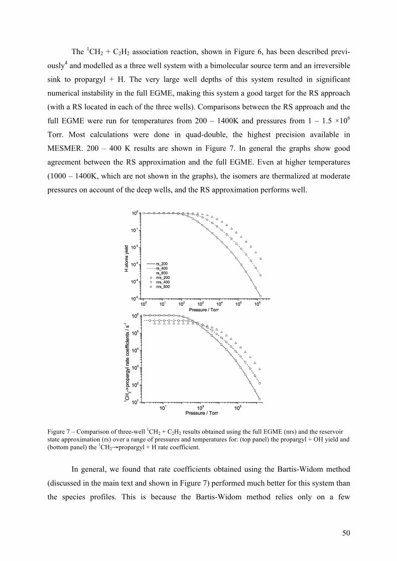
50

The 1CH2 + C2H2 association reaction, shown in Figure 6, has been described previ-

ously4 and modelled as a three well system with a bimolecular source term and an irreversible

sink to propargyl + H. The very large well depths of this system resulted in significant

numerical instability in the full EGME, making this system a good target for the RS approach

(with a RS located in each of the three wells). Comparisons between the RS approach and the

full EGME were run for temperatures from 200 – 1400K and pressures from 1 – 1.5 ×106

Torr. Most calculations were done in quad-double, the highest precision available in

MESMER. 200 – 400 K results are shown in Figure 7. In general the graphs show good

agreement between the RS approximation and the full EGME. Even at higher temperatures

(1000 – 1400K, which are not shown in the graphs), the isomers are thermalized at moderate

pressures on account of the deep wells, and the RS approximation performs well.

Figure 7 – Comparison of three-well 1CH2 + C2H2 results obtained using the full EGME (nrs) and the reservoir state approximation (rs) over a range of pressures and temperatures for: (top panel) the propargyl + OH yield and (bottom panel) the 1CH2→propargyl + H rate coefficient.

In general, we found that rate coefficients obtained using the Bartis-Widom method

(discussed in the main text and shown in Figure 7) performed much better for this system than

the species profiles. This is because the Bartis-Widom method relies only on a few

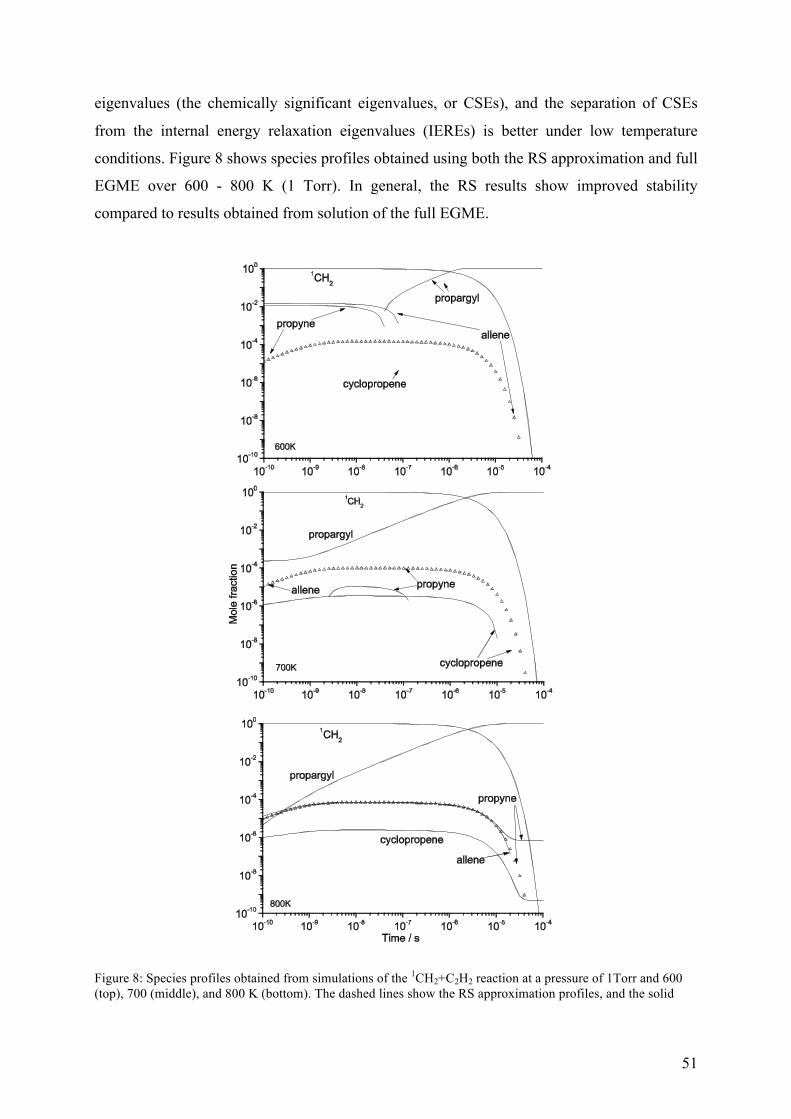
51

eigenvalues (the chemically significant eigenvalues, or CSEs), and the separation of CSEs

from the internal energy relaxation eigenvalues (IEREs) is better under low temperature

conditions. Figure 8 shows species profiles obtained using both the RS approximation and full

EGME over 600 - 800 K (1 Torr). In general, the RS results show improved stability

compared to results obtained from solution of the full EGME.

Figure 8: Species profiles obtained from simulations of the 1CH2+C2H2 reaction at a pressure of 1Torr and 600 (top), 700 (middle), and 800 K (bottom). The dashed lines show the RS approximation profiles, and the solid

52

lines show the data obtained from solution of the full EGME. The allene population from the RS approximation is marked by unfilled triangles to avoid ambiguity.

Finally we note that, compared to the time required to solve the full EGME for this

system, the RS approximation introduces a factor of eight computational speed-up owing to

reduction in size of the matrix to be diagonalized.

6. References

1. Robertson, S. H.; Pilling, M. J.; Jitariu, L. C.; Hillier, I. H. Phys Chem Chem Phys 2007, 9(31), 4085-4097. 2. McKee, K. W.; Blitz, M. A.; Cleary, P. A.; Glowacki, D. R.; Pilling, M. J.; Seakins, P. W.; Wang, L. J Phys Chem A 2007, 111(19), 4043-4055. 3. Carr, S. A.; Glowacki, D. R.; Liang, C. H.; Baeza-Romero, M. T.; Blitz, M. A.; Pilling, M. J.; Seakins, P. W. J Phys Chem A 2011, 115(6), 1069-1085. 4. Gannon, K. L.; Blitz, M. A.; Liang, C. H.; Pilling, M. J.; Seakins, P. W.; Glowacki, D. R. J Phys Chem A 2010, 114(35), 9413-9424.