Magnetic Resonance Imaging 33 (2015) 146–160

Contents lists available at ScienceDirect

Magnetic Resonance Imaging

j ourna l homepage: www.mr i journa l .com

Meshless deformable models for 3D cardiac motion and strain

analysis from tagged MRI

Xiaoxu Wang a,⁎, Ting Chen d, Shaoting Zhang b, Joël Schaerer c, Zhen Qian b, Suejung Huh b,Dimitris Metaxas b, Leon Axel d

a Shenzhen Institute of Advance Technology, CAS, Xueyuan Ave. 1068, Xili, Nanshan, Shenzhen, Guangdong, China, 518055b Department of Computer Science, Rutgers University, 110 Frelinghuysen Rd, Piscataway, NJ, 08854, USAc CREATIS, INSA LYON, Bâtiment Blaise Pascal, 7 Avenue Jean Capelle, 69621, Villeurbanne Cedex, Franced Radiology Department, New York University, 660 first Avenue, New York, NY, 10016, USA

⁎ Corresponding author.E-mail address: wang.xx@siat.ac.cn (X. Wang).

http://dx.doi.org/10.1016/j.mri.2014.08.0070730-725X/© 2014 Published by Elsevier Inc.

a b s t r a c t

a r t i c l e i n f o

Article history:Received 28 June 2013Revised 28 May 2014Accepted 8 August 2014

Keywords:MRIDeformable modelsMotion trackingStrainCardiac

Tagged magnetic resonance imaging (TMRI) provides a direct and noninvasive way to visualize the in-walldeformation of the myocardium. Due to the through-plane motion, the tracking of 3D trajectories of thematerial points and the computation of 3D strain field call for the necessity of building 3D cardiacdeformable models. The intersections of three stacks of orthogonal tagging planes are material points inthe myocardium. With these intersections as control points, 3D motion can be reconstructed with a novelmeshless deformable model (MDM). Volumetric MDMs describe an object as point cloud inside the objectboundary and the coordinate of each point can be written in parametric functions. A generic heart mesh isregistered on the TMRI with polar decomposition. A 3D MDM is generated and deformed with MR imagetagging lines. Volumetric MDMs are deformed by calculating the dynamics function and minimizing thelocal Laplacian coordinates. The similarity transformation of each point is computed by assuming itsneighboring points are making the same transformation. The deformation is computed iteratively until thecontrol points match the target positions in the consecutive image frame. The 3D strain field is computedfrom the 3D displacement field with moving least squares. We demonstrate that MDMs outperformed thefinite element method and the spline method with a numerical phantom. Meshless deformable models cantrack the trajectory of any material point in the myocardium and compute the 3D strain field of anyparticular area. The experimental results on in vivo healthy and patient heart MRI show that the MDM canfully recover the myocardium motion in three dimensions.

© 2014 Published by Elsevier Inc.

1. Introduction

Tagged magnetic resonance imaging (TMRI) is a non-invasive wayto track the in-wall in vivomyocardiummotion during a cardiac cycle.Conventional MRI can only show the boundary of the ventricles. Thenumber of natural occurring landmarks that can be reliably identifiedon the ventricle boundaries is limited. Axel and Dougherty [1]developed a tagging technique called spatial modulation of magneti-zation (SPAMM),which can produce saturated parallel planes throughentire imaging volumewithin a fewmilliseconds comparedwith otherTMRI methods [2–4]. Van der Paardt et al. [5] and Tustison et al. [6]utilize these methods on other organ imaging.

The application of MRI tagging technique on cardiac motionimaging is elaborated and left ventricle circumferential shorteningmotion scale is measured in different parts of the ventricle wall in

paper McVeigh et al. [7]. Cardiac motion of left ventricle of healthyvolunteers is tracked on the tagged short axis MRI in paper Sampathand Prince [8]. Two dimensional (2D) motion is validated on a pulsesequence phantom. The motion is combined with long axis imagewith 2D pathline and the left ventricle strain on short axis MRI iscalculated in paper Sampath and Prince [9]. The TMRI of nine caninehearts with ischemia is analyzed and demonstrated that TMRI candetect ischemia of the left ventricle in paper Denisova et al. [10]. Theability of motion tracking of cine phase-contrast magnetic resonanceis validated with an in vitro model in paper Drangova et al. [11]. Theheart failure could be early diagnosed and prevented with leftventricle dysfunction analysis with MRI. The aortic stiffness and themyocardial strain irregular are found to be highly related in paperIbrahim et al. [12].

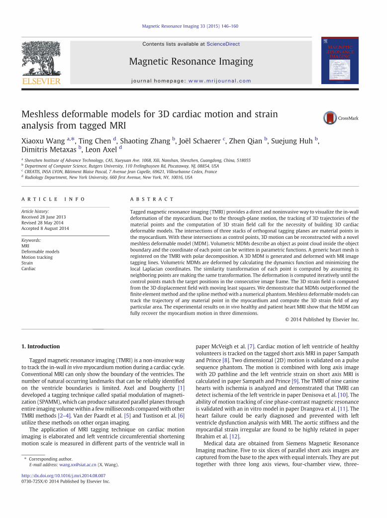
Medical data are obtained from Siemens Magnetic ResonanceImaging machine. Five to six slices of parallel short axis images arecaptured from the base to the apex with equal intervals. They are puttogether with three long axis views, four-chamber view, three-

147X. Wang et al. / Magnetic Resonance Imaging 33 (2015) 146–160

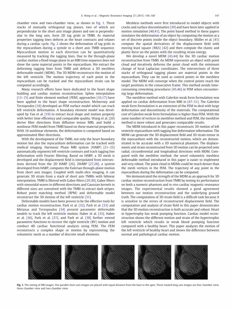
chamber view and two-chamber view, as shown in Fig. 1. Threestacks of mutually orthogonal tag planes, two of which areperpendicular to the short axis image planes and one is perpendic-ular to the long axis, form 2D tag grids in TMRI. As materialproperties tagging lines deform as the heart contracts and relaxesduring a cardiac cycle. Fig. 2 shows the deformation of tag grids inthe myocardium during a systole in a short axis TMRI sequence.Myocardium motion in each direction can be quantitativelymeasured by tracking the tagging lines. Due to the through-planecardiacmotion a fixed image plane in anMRI time sequence does notshow the same material points in the myocardium. We extract thedeforming tagging lines from TMRI and deform a 3D meshlessdeformable model (MDM). The 3D MDM reconstructs the motion ofthe left ventricle. The motion trajectory of each point in themyocardium can be tracked and the myocardium strain can becomputed accordingly.

Many research efforts have been dedicated to the heart shapebuilding and cardiac motion reconstruction. Spline interpolation[13–15] and finite element method (FEM) approaches [16,17] havebeen applied to the heart shape reconstruction. McInerney andTerzopoulos [18] developed an FEM surface model which can trackleft ventricle deformation. A boundary element model was devel-oped by Yan et al. [19] to extract local shape and motion propertywith better time efficiency and comparable quality. Wang et al. [20]derive fiber directions from diffusion tensor MRI, and build anonlinear FEMmodel from TMRI based on these material properties.With 16 nonlinear elements, the deformation is computed based onapproximated fiber directions.

With the development of the TMRI, not only the heart boundarymotion but also the myocardium deformation can be tracked withmedical imaging. Harmonic Phase MRI system (HARP) [21–25]automatically segments left ventricle contours and track tagging linedeformation with Fourier filtering. Based on HARP, a 3D mesh isdeveloped and the displacement field is interpolated from intersec-tions derived from the 2D HARP [26]. ZHARP [27,28], a systemdeveloped from HARP, computes the Eulerian through-plane motionfrom short axis images. Coupled with multi-slice imaging, it cangenerate 3D strain from a stack of short axis TMRIs with bilinearinterpolation. TMRI is filtered with Gabor filters [29,30]. Gabor filterswith sinosoidal waves in different directions and Gaussian kernels indifferent sizes are convolved with the TMRI to extract dark stripes.Robust point matching method (RPM) and deformable modelreconstruct the 3D motion of the left ventricle [31].

Deformable models have been proven to be the effective tools forcardiac motion reconstruction. Park et al. [32], Park et al. [33] andMetaxas and Terzopoulos [34] present parameter deformablemodels to track the left ventricle motion. Haber et al. [35], Haberet al. [36], Park et al. [37], and Park et al. [38] further extendparametric functions to recover the right ventricle (RV) motion andconduct 4D cardiac functional analysis using FEM. The FEMreconstructs a complex shape or motion by representing thevolumetric mesh as a number of discrete small elements.

Fig. 1. The setting of MR images: five parallel short axis images are placed with equal distathree chamber view and two chamber view.

Meshless methods were first introduced to model objects withcracks and surface discontinuities [39] and have been later applied inmotion simulation [40,41]. The point based method in these paperssimulates the deformation of an object by computing the motion at aset of discrete points inside the object boundary. Müller et al. [41]compute the spatial derivatives of the displacement field withmoving least square (MLS) [42] and then compute the elastic andplastic force on the points with the resulting strain energy.

We develop a novel MDM [43,44] for the 3D cardiac motionreconstruction from TMRI. An MDM represents an object with pointcloud and iteratively deforms the point cloud with the minimumchange of local Laplacian coordinates. The intersections of threestacks of orthogonal tagging planes are material points in themyocardium. They can be used as control points in the meshlessmodel. The MDM will converge when the control points reach thetarget positions in the consecutive frame. This method avoids time-consuming remeshing procedures [45,46] in FEM when encounter-ing large deformation.

The meshfree method with Galerkin weak form formulation wasapplied on cardiac deformation from MRI in [47–51]. The Galerkinweak form formulation is an extension of the FEM to deal with largedeformation and discontinuity of the materials. The computationalcost of Galerkin weak form formulation is higher than FEM. With thesame number of vertices in meshfree method and FEM, themeshfreemethod is more robust and generates comparable results.

The MDM introduced in this paper reconstructs 3D motion of leftventricle myocardiumwith tagging line deformation information. TheMDM can generate the 3D displacement field and 3D strain tensor inthe myocardium with the reconstructed motion, which are demon-strated to be accurate with a 3D numerical phantom. The displace-ments and strain reconstructed from 3Dmotion can be projected ontoradial, circumferential and longitudinal directions with MDM. Com-pared with the meshfree method, the novel volumetric meshlessdeformable method introduced in this paper is easier to implementand very robust. The point cloud in MDMs could bemuch denser thanthe mesh vertices in the FEM. The trajectory of any point in themyocardium during the deformation can be computed.

We demonstrated the strength of theMDM as an approach for 3Dcardiac motion reconstruction from TMRI by testing its performanceon both a numeric phantom and in vivo cardiac magnetic resonanceimages. The experimental results showed a good agreementbetween our motion reconstruction and the underlying groundtruth. The computation of 3D strain field is a difficult task because itis sensitive to the errors of reconstructed displacement field. Thecomputation and analysis of strain field in this paper demonstratesthat the 3D motion reconstruction is both accurate and robust. Heartin hypertrophy has weak pumping function. Cardiac model recon-struction shows the different motion and strain of the hypertrophicleft ventricle which results in weak blood pumping functioncompared with a healthy heart. This paper analyzes the motion ofthe left ventricle of healthy heart and shows the difference betweennormal and pathological cardiac motion.

nce from the base to the apex. Three rotated long axis images are four chamber view

,

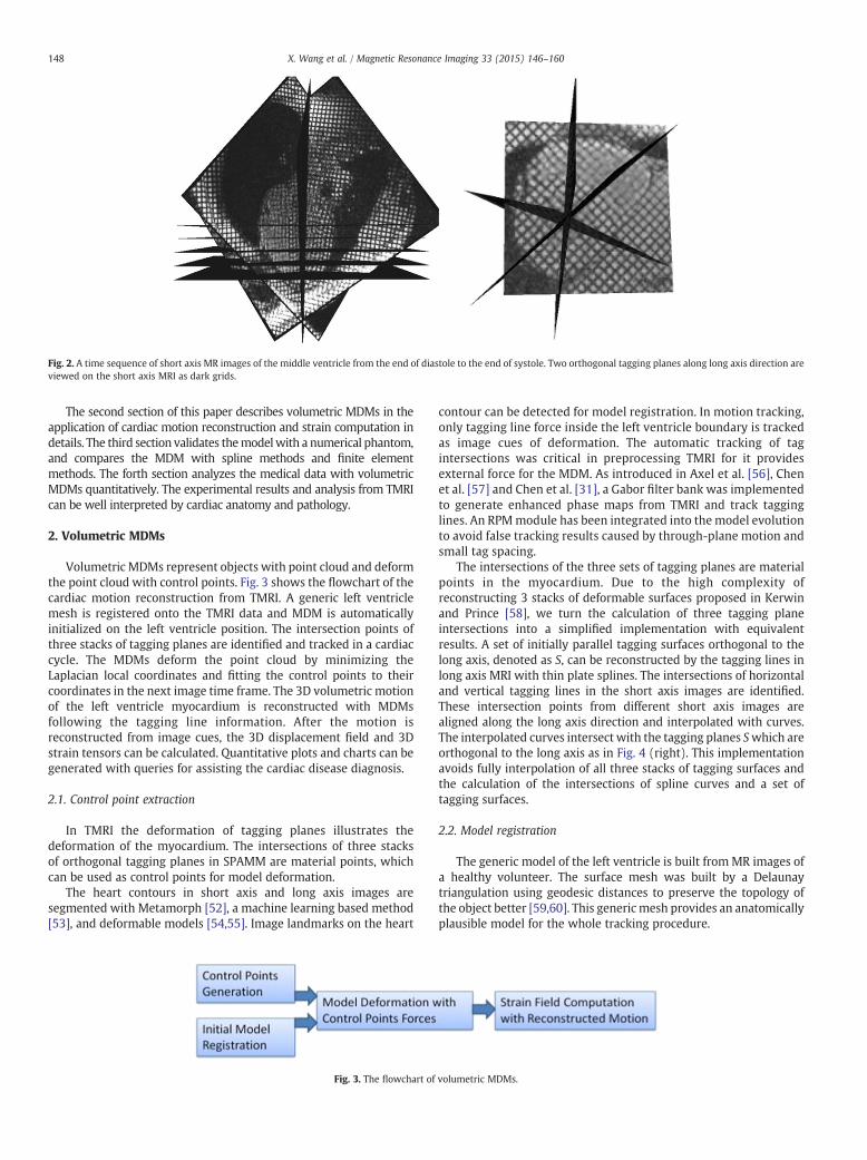
Fig. 2. A time sequence of short axis MR images of the middle ventricle from the end of diastole to the end of systole. Two orthogonal tagging planes along long axis direction areviewed on the short axis MRI as dark grids.

148 X. Wang et al. / Magnetic Resonance Imaging 33 (2015) 146–160

The second section of this paper describes volumetric MDMs in theapplication of cardiac motion reconstruction and strain computation indetails. The third section validates themodelwith a numerical phantom,and compares the MDM with spline methods and finite elementmethods. The forth section analyzes the medical data with volumetricMDMs quantitatively. The experimental results and analysis from TMRIcan be well interpreted by cardiac anatomy and pathology.

2. Volumetric MDMs

Volumetric MDMs represent objects with point cloud and deformthe point cloud with control points. Fig. 3 shows the flowchart of thecardiac motion reconstruction from TMRI. A generic left ventriclemesh is registered onto the TMRI data and MDM is automaticallyinitialized on the left ventricle position. The intersection points ofthree stacks of tagging planes are identified and tracked in a cardiaccycle. The MDMs deform the point cloud by minimizing theLaplacian local coordinates and fitting the control points to theircoordinates in the next image time frame. The 3D volumetric motionof the left ventricle myocardium is reconstructed with MDMsfollowing the tagging line information. After the motion isreconstructed from image cues, the 3D displacement field and 3Dstrain tensors can be calculated. Quantitative plots and charts can begenerated with queries for assisting the cardiac disease diagnosis.

2.1. Control point extraction

In TMRI the deformation of tagging planes illustrates thedeformation of the myocardium. The intersections of three stacksof orthogonal tagging planes in SPAMM are material points, whichcan be used as control points for model deformation.

The heart contours in short axis and long axis images aresegmented with Metamorph [52], a machine learning based method[53], and deformable models [54,55]. Image landmarks on the heart

Fig. 3. The flowchart of volumetric MDMs.

contour can be detected for model registration. In motion tracking,only tagging line force inside the left ventricle boundary is trackedas image cues of deformation. The automatic tracking of tagintersections was critical in preprocessing TMRI for it providesexternal force for the MDM. As introduced in Axel et al. [56], Chenet al. [57] and Chen et al. [31], a Gabor filter bank was implementedto generate enhanced phase maps from TMRI and track tagginglines. An RPMmodule has been integrated into the model evolutionto avoid false tracking results caused by through-plane motion andsmall tag spacing.

The intersections of the three sets of tagging planes are materialpoints in the myocardium. Due to the high complexity ofreconstructing 3 stacks of deformable surfaces proposed in Kerwinand Prince [58], we turn the calculation of three tagging planeintersections into a simplified implementation with equivalentresults. A set of initially parallel tagging surfaces orthogonal to thelong axis, denoted as S, can be reconstructed by the tagging lines inlong axis MRI with thin plate splines. The intersections of horizontaland vertical tagging lines in the short axis images are identified.These intersection points from different short axis images arealigned along the long axis direction and interpolated with curves.The interpolated curves intersect with the tagging planes Swhich areorthogonal to the long axis as in Fig. 4 (right). This implementationavoids fully interpolation of all three stacks of tagging surfaces andthe calculation of the intersections of spline curves and a set oftagging surfaces.

2.2. Model registration

The generic model of the left ventricle is built fromMR images ofa healthy volunteer. The surface mesh was built by a Delaunaytriangulation using geodesic distances to preserve the topology ofthe object better [59,60]. This generic mesh provides an anatomicallyplausible model for the whole tracking procedure.

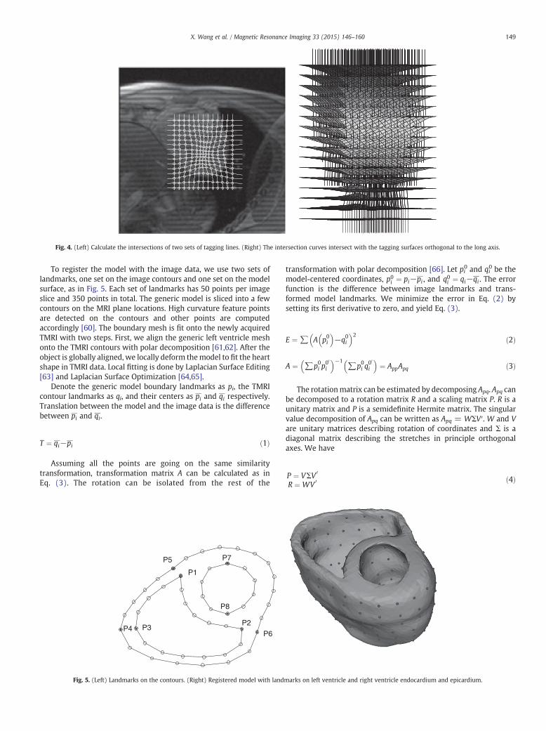
Fig. 4. (Left) Calculate the intersections of two sets of tagging lines. (Right) The intersection curves intersect with the tagging surfaces orthogonal to the long axis.

149X. Wang et al. / Magnetic Resonance Imaging 33 (2015) 146–160

To register the model with the image data, we use two sets oflandmarks, one set on the image contours and one set on the modelsurface, as in Fig. 5. Each set of landmarks has 50 points per imageslice and 350 points in total. The generic model is sliced into a fewcontours on the MRI plane locations. High curvature feature pointsare detected on the contours and other points are computedaccordingly [60]. The boundary mesh is fit onto the newly acquiredTMRI with two steps. First, we align the generic left ventricle meshonto the TMRI contours with polar decomposition [61,62]. After theobject is globally aligned, we locally deform themodel to fit the heartshape in TMRI data. Local fitting is done by Laplacian Surface Editing[63] and Laplacian Surface Optimization [64,65].

Denote the generic model boundary landmarks as pi, the TMRIcontour landmarks as qi, and their centers as pi and qi respectively.Translation between the model and the image data is the differencebetween pi and qi.

T ¼ qi−pi ð1Þ

Assuming all the points are going on the same similaritytransformation, transformation matrix A can be calculated as inEq. (3). The rotation can be isolated from the rest of the

P1

P2

P7P5

P6P4 P3

P8

Fig. 5. (Left) Landmarks on the contours. (Right) Registered model with landmarks on left ventricle and right ventricle endocardium and epicardium.

transformation with polar decomposition [66]. Let pi0 and qi0 be the

model-centered coordinates, p0i ¼ pi−pi , and q0i ¼ qi−qi . The errorfunction is the difference between image landmarks and trans-formed model landmarks. We minimize the error in Eq. (2) bysetting its first derivative to zero, and yield Eq. (3).

E ¼ ∑ A p0i� �

−q0i� �2 ð2Þ

A ¼ ∑p0i p00

i

� �−1∑p0i q

00

i

� �¼ AppApq ð3Þ

The rotationmatrix can be estimated by decomposing Apq. Apq canbe decomposed to a rotation matrix R and a scaling matrix P. R is aunitary matrix and P is a semidefinite Hermite matrix. The singularvalue decomposition of Apq can be written as Apq = WΣV′. W and Vare unitary matrices describing rotation of coordinates and Σ is adiagonal matrix describing the stretches in principle orthogonalaxes. We have

P ¼ VΣV 0

R ¼ WV 0 ð4Þ

150 X. Wang et al. / Magnetic Resonance Imaging 33 (2015) 146–160

Thematrix P is always unique. V and Σ can be computed by the Eigendecomposition of Apq′Apq directly based on Eq. (5).

P ¼ffiffiffiffiffiffiffiffiffiffiffiffiffiffiffiffiApq′Apq

q¼

ffiffiffiffiffiffiffiffiffiffiffiffiffiffiffiffiffiffiffiffiffiffiffiffiffiffiffiffiffiffiffiffiffiffiVΣW 0ð Þ WΣV 0ð Þ

q¼

ffiffiffiffiffiffiffiffiffiffiffiffiffiffiffiffiffiffiV Σð Þ2V 0

qð5Þ

P−1 ¼ V 1=Σð ÞV 0 ð6Þ

If A is invertible, the inverse of P can be calculated by substituting Vand Σ into Eq. (6). The rotationmatrix of registration can be calculatedby substituting Eq. (6) into R = ApqP

−1. After obtaining translationand rotation, uniform scaling can be computed by comparing theaverage magnitude of vectors in the object-centered coordinates.

3. Model initialization

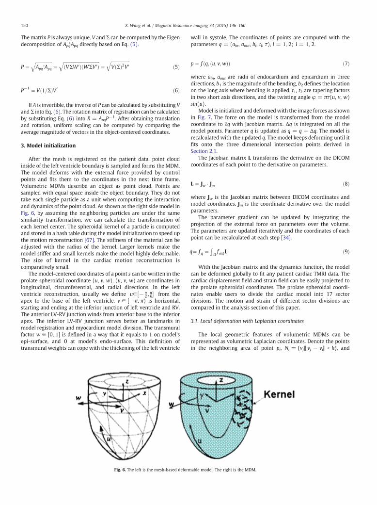
After the mesh is registered on the patient data, point cloudinside of the left ventricle boundary is sampled and forms the MDM.The model deforms with the external force provided by controlpoints and fits them to the coordinates in the next time frame.Volumetric MDMs describe an object as point cloud. Points aresampled with equal space inside the object boundary. They do nottake each single particle as a unit when computing the interactionand dynamics of the point cloud. As shown as the right side model inFig. 6, by assuming the neighboring particles are under the samesimilarity transformation, we can calculate the transformation ofeach kernel center. The spheroidal kernel of a particle is computedand stored in a hash table during the model initialization to speed upthe motion reconstruction [67]. The stiffness of the material can beadjusted with the radius of the kernel. Larger kernels make themodel stiffer and small kernels make the model highly deformable.The size of kernel in the cardiac motion reconstruction iscomparatively small.

The model-centered coordinates of a point s can be written in theprolate spheroidal coordinate (u, v, w). (u, v, w) are coordinates inlongitudinal, circumferential, and radial directions. In the leftventricle reconstruction, usually we define u∈ − π

2 ;π6

� �from the

apex to the base of the left ventricle. v ∈ [−π, π) is horizontal,starting and ending at the inferior junction of left ventricle and RV.The anterior LV-RV junction winds from anterior base to the inferiorapex. The inferior LV-RV junction serves better as landmarks inmodel registration and myocardium model division. The transmuralfactor w ∈ [0, 1] is defined in a way that it equals to 1 on model'sepi-surface, and 0 at model's endo-surface. This definition oftransmural weights can cope with the thickening of the left ventricle

Fig. 6. The left is the mesh-based deformable model. The right is the MDM.

wall in systole. The coordinates of points are computed with theparameters q = (ain, aout, bi, tl, τ), i = 1, 2; l = 1, 2.

p ¼ f q; u; v;wð Þð Þ ð7Þ

where ain, aout are radii of endocardium and epicardium in threedirections, b1 is themagnitude of the bending, b2 defines the locationon the long axis where bending is applied, t1, t2 are tapering factorsin two short axis directions, and the twisting angle φ = πτ(u, v, w)sin(u).

Model is initialized and deformedwith the image forces as shownin Fig. 7. The force on the model is transformed from the modelcoordinate to δq with Jacobian matrix. Δq is integrated on all themodel points. Parameter q is updated as q = q + Δq. The model isrecalculated with the updated q. The model keeps deforming until itfits onto the three dimensional intersection points derived inSection 2.1.

The Jacobian matrix L transforms the derivative on the DICOMcoordinates of each point to the derivative on parameters.

L ¼ Jw � Jm ð8Þ

where Jw is the Jacobian matrix between DICOM coordinates andmodel coordinates. Jm is the coordinate derivative over the modelparameters.

The parameter gradient can be updated by integrating theprojection of the external force on parameters over the volume.The parameters are updated iteratively and the coordinates of eachpoint can be recalculated at each step [34].

q̇¼ f q ¼ ∫Ωf extL ð9Þ

With the Jacobian matrix and the dynamics function, the modelcan be deformed globally to fit any patient cardiac TMRI data. Thecardiac displacement field and strain field can be easily projected tothe prolate spheroidal coordinates. The prolate spheroidal coordi-nates enable users to divide the cardiac model into 17 sectordivisions. The motion and strain of different sector divisions arecompared in the analysis section of this paper.

3.1. Local deformation with Laplacian coordinates

The local geometric features of volumetric MDMs can berepresented as volumetric Laplacian coordinates. Denote the pointsin the neighboring area of point pi, Ni = {vj|‖vj − vi‖ b h}, and

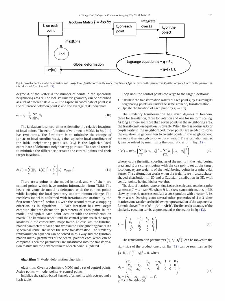
Fig. 7. Flowchart of themodel deformation with image force. fx is the force on themodel coordinates. fq is the force on the parameters. Fq is the integrated force on the parameters.L is calculated from J as in Eq. (8).

151X. Wang et al. / Magnetic Resonance Imaging 33 (2015) 146–160

degree di of the vertex is the number of points in the spheroidalneighboring area Ni. The local volumetric geometry can be describedas a set of differentials Δ = δi. The Laplacian coordinate of point vi isthe difference between point vi and the average of its neighbors

δi ¼ vi−1di

Xj∈N við Þ

vj ð10Þ

The Laplacian local coordinates describe the relative locationsof local points. The error function of volumetric MDMs in Eq. (11)has two terms. The first term is to minimize the change ofLaplacian local coordinates. δi is the Laplacian local coordinate ofthe initial neighboring point set. L(vi′) is the Laplacian localcoordinate of deformed neighboring point set. The second term isto minimize the difference between the control points and theirtarget locations.

E V 0� � ¼Xni¼1

jjδi−L v0i� �jj2 þXm

j¼1

jv0j−vtarget jj2 ð11Þ

There are n points in the model in total, and m of them arecontrol points which have motion information from TMRI. Theheart left ventricle model is deformed with the control pointswhile keeping the local geometry underminimum change. Themeshless model is deformed with iterations constrained by thefirst term of error function 11, with the second term as a stoppingcriterion, as in algorithm 11. Each iteration has two steps:compute the transformation parameters of each point in themodel; and update each point location with the transformationmatrix. The iterations repeat until the control points reach the targetlocations in the consecutive image frame. To calculate the transfor-mationparameters of eachpoint,we assume itsneighboringpoints in aspheroidal kernel are under the same transformation. The similaritytransformation equation can be solved in this way and the transfor-mation matrix parameters of the central point of each kernel can becomputed. Then the parameters are substituted into the transforma-tion matrix and the new coordinate of each point is updated.

Algorithm 1. Model deformation algorithm

Algorithm: Given a volumetric MDM and a set of control points.Active points = model points + control points.

Initialize the radius-based kernels of all points with octrees and ahash table.

Loop until the control points converge to the target locations:

1. Calculate the transformation matrix of each point Ti by assuming itsneighboring points are under the same similarity transformation;

2. Update the location of each point by xi = Tix i′.

The similarity transformation has seven degrees of freedom,three for translation, three for rotation and one for uniform scaling.As long as there are more than seven points in the neighboring area,the transformation equation is solvable.When there is co-linearity orco-planarity in the neighborhood, more points are needed to solvethe equation. In general, ten to twenty points in the neighborhoodare more than enough to solve the equation. Transformation matrixTi can be solved by minimizing the quadratic error in Eq. (12).

E V 0� � ¼ minTi

X1

Tivi−v0i 2 þX

j∈Ni

wj Tiv j−v0j 2

0@ 1A ð12Þ

where vis are the initial coordinates of the points in the neighboringarea, and vi′ are current points with the cue points set at the targetlocations. wj are weights of the neighboring points in a spheroidalkernel. The deformation works when the weights are in a parachute-shaped distribution in 2D and a Gaussian distribution in 3D, withcentral points having higher weights.

The class ofmatrices representing isotropic scales and rotation canbewritten as T = s ⋅ exp(H), where H is a skew-symmetric matrix. In 3D,skew-symmetric matrices emulate a cross product with a vector h, i.e.Hx = h × x. Drawing upon several other properties of 3 × 3 skewmatrices, one can derive the following representation of the exponentialformula above: Ti = s(αI + βH + γhTh). Thefirst order accuracy of thesimilarity equation can be approximated as the matrix in Eq. (13).

Ti ¼s −h3 h2 txh3 s h1 ty−h2 h1 s tz0 0 0 1

0BB@1CCA ð13Þ

The transformation parameters si;hiT; tiT

� �Tcan be moved to the

right side of the product operator. Eq. (12) can be rewritten as jjAi

si;hiT; tiT

� �T−bijj2 ¼ 0, where

Ai ¼xk1 0 xk3 −xk2 1 0 0xk2 −xk3 0 xk1 0 1 0xk3 xk2 −xk1 0 0 0 1⋮

0BB@1CCA;

bi ¼ xk1 ′ xk2 ′ xk3 ′ …� �0

;

k ∈ i ∪ Neighbor ið Þ

ð14Þ

152 X. Wang et al. / Magnetic Resonance Imaging 33 (2015) 146–160

The matrix Ai has the initial locations V of all points in theneighboring area of vi, and can be computed before the iteration. Thevector bi has the current points and the expected coordinates of thecontrol points, denote as V′. Once the similarity transformationparameters of each point are calculated by solving the linear system(Eq. (14)), we can update each point coordinate with the transforma-tion matrix. The volumetric point cloud deforms with the externalforce on the control points iteratively. A model with seven thousandpoints can deform to its target shape in a few minutes.

3.2. Strain computation

After the motion is reconstructed with volumetric MDMs, a 3Ddisplacement field can be computed by comparing the model in twoMRI frames. The strain field of the myocardium during the systoleshows the myocardium contraction and blood pumping ability.Strain describes the relative deformation, such as local stretch andcompression of the myocardium. The myocardial strain pattern of apatient's heart is different from that of a healthy heart. The strainfield of the myocardium could help in detecting scars resulted fromcardiac ischemia and infarction.

Given the initial position of a point x0 = (x, y, z) in a worldcoordinate and the displacement u(t) = (ux, uy, uz) at time t, thecurrent position of the point in the deformedmodel is x(t) = x0 + u(t).The Jacobian of this mapping is

J ¼ I þ∇uT ¼1þ ux;x ux;y ux;zuy;x 1þ uy;y uy;zuz;x uz;y 1þ uz;z

24 35 ð15Þ

For instance, ux,y is the gradient of the displacement u's xcomponent on y direction, ∂ux/∂y. Given the Jacobian J, theLagrangian strain tensor ε of the point can be approximated withGreen's strain tensor

ε ¼ 12

JT J−I� �

¼ 12

∇uþ∇uT þ∇u∇uT� �

ð16Þ

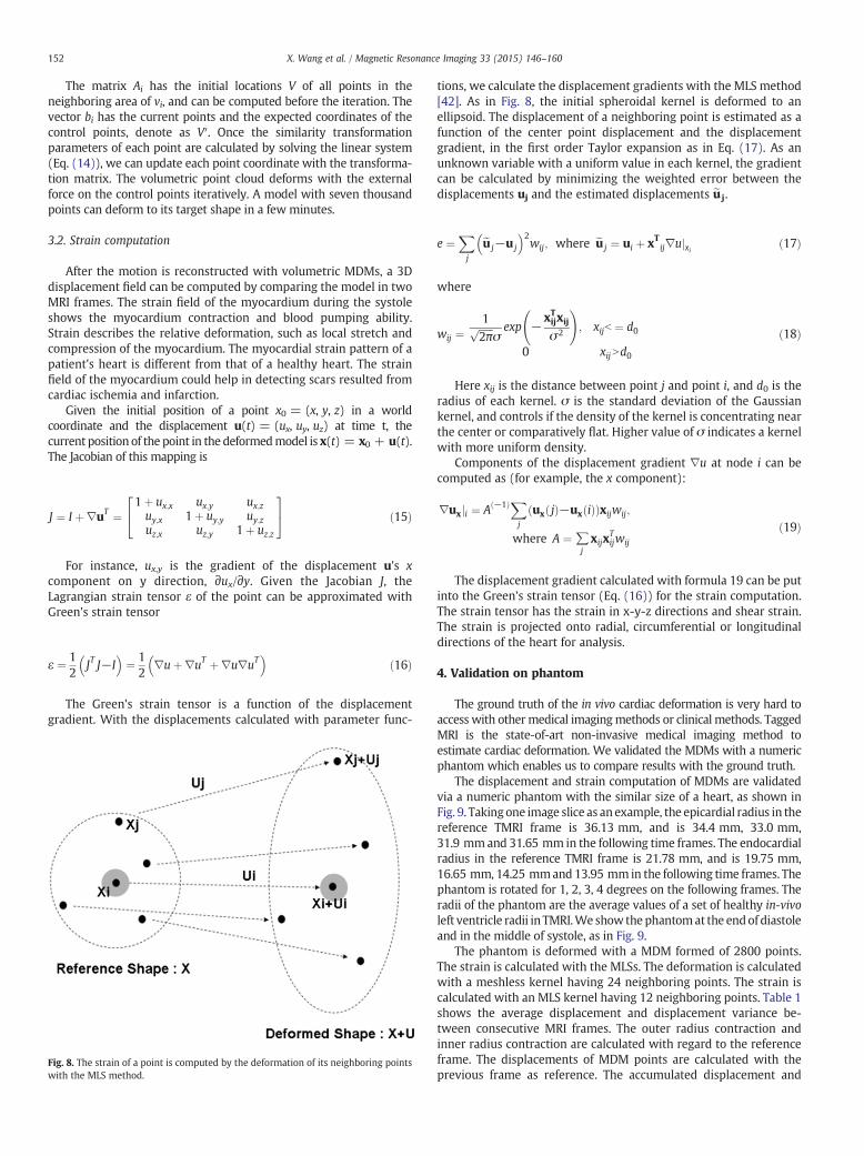
The Green's strain tensor is a function of the displacementgradient. With the displacements calculated with parameter func-

ig. 8. The strain of a point is computed by the deformation of its neighboring pointsith the MLS method.

Fw

tions, we calculate the displacement gradients with the MLS method[42]. As in Fig. 8, the initial spheroidal kernel is deformed to anellipsoid. The displacement of a neighboring point is estimated as afunction of the center point displacement and the displacementgradient, in the first order Taylor expansion as in Eq. (17). As anunknown variable with a uniform value in each kernel, the gradientcan be calculated by minimizing the weighted error between thedisplacements uj and the estimated displacements euj.

e ¼Xj

eu j−u j

� �2wij; where eu j ¼ ui þ xT

ij∇ujxi ð17Þ

where

wij ¼1ffiffiffiffiffiffi2π

pσexp −

xTijxij

σ2

!; xijb ¼ d0

0 xijNd0

ð18Þ

Here xij is the distance between point j and point i, and d0 is theradius of each kernel. σ is the standard deviation of the Gaussiankernel, and controls if the density of the kernel is concentrating nearthe center or comparatively flat. Higher value of σ indicates a kernelwith more uniform density.

Components of the displacement gradient ∇u at node i can becomputed as (for example, the x component):

∇uxji ¼ A −1ð ÞXj

ux jð Þ−ux ið Þð Þxijwij;

where A ¼ ∑jxijx

Tijwij

ð19Þ

The displacement gradient calculated with formula 19 can be putinto the Green's strain tensor (Eq. (16)) for the strain computation.The strain tensor has the strain in x-y-z directions and shear strain.The strain is projected onto radial, circumferential or longitudinaldirections of the heart for analysis.

4. Validation on phantom

The ground truth of the in vivo cardiac deformation is very hard toaccess with othermedical imagingmethods or clinical methods. TaggedMRI is the state-of-art non-invasive medical imaging method toestimate cardiac deformation. We validated the MDMs with a numericphantom which enables us to compare results with the ground truth.

The displacement and strain computation of MDMs are validatedvia a numeric phantom with the similar size of a heart, as shown inFig. 9. Taking one image slice as anexample, the epicardial radius in thereference TMRI frame is 36.13 mm, and is 34.4 mm, 33.0 mm,31.9 mmand 31.65 mm in the following time frames. The endocardialradius in the reference TMRI frame is 21.78 mm, and is 19.75 mm,16.65 mm, 14.25 mmand 13.95 mm in the following time frames. Thephantom is rotated for 1, 2, 3, 4 degrees on the following frames. Theradii of the phantom are the average values of a set of healthy in-vivoleft ventricle radii in TMRI.We show thephantomat the endof diastoleand in the middle of systole, as in Fig. 9.

The phantom is deformed with a MDM formed of 2800 points.The strain is calculated with the MLSs. The deformation is calculatedwith a meshless kernel having 24 neighboring points. The strain iscalculated with an MLS kernel having 12 neighboring points. Table 1shows the average displacement and displacement variance be-tween consecutive MRI frames. The outer radius contraction andinner radius contraction are calculated with regard to the referenceframe. The displacements of MDM points are calculated with theprevious frame as reference. The accumulated displacement and

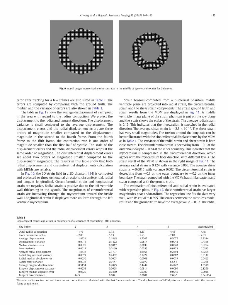
Fig. 9. A grid tagged numeric phantom contracts in the middle of systole and rotates for 2 degrees.

153X. Wang et al. / Magnetic Resonance Imaging 33 (2015) 146–160

error after tracking for a few frames are also listed in Table 1. Theerrors are computed by comparing with the ground truth. Themedian and the variance of errors are also shown in Table 1.

The table in Fig. 1 shows the average displacement of each pointin the area with regard to the radius contraction. We project thedisplacement to the radial and tangent directions. The displacementvariance is small compared to the average displacement. Thedisplacement errors and the radial displacement errors are threeorders of magnitude smaller compared to the displacementmagnitude in the second to the fourth frame. From the fourthframe to the fifth frame, the contraction rate is one order ofmagnitude smaller than the first half of systole. The scale of thedisplacement errors and the radial displacement errors keeps at thesame order of magnitude. The circumferential displacement errorsare about two orders of magnitude smaller compared to thedisplacement magnitude. The results in this table show that bothradial displacements and circumferential displacements calculationwith MDMs are reliable.

In Fig. 10, the 3D strain field in a 3D phantom [34] is computedand projected to three orthogonal directions, circumferential, radialand tangent longitudinal. Circumferential strain and longitudinalstrain are negative. Radial strain is positive due to the left ventriclewall thickening in the systole. The magnitudes of circumferentialstrain are increasing through the myocardium toward the insidewall. Longitudinal strain is displayed more uniform through the leftventricle myocardium.

Table 1Displacement results and errors in millimeters of a sequence of contracting TMRI phantom.

Key frame 2 3 4 5 Accumulated

Outer radius contraction −1.73 −3.13 −4.23 −4.48 −4.48Inner radius contraction −2.03 −5.13 −7.53 −7.83 −7.83Average displacement 1.9324 2.1845 1.7203 0.5077 6.2314Displacement variance 0.0018 0.1472 0.0814 0.0043 0.4326Median absolute error 0.0028 0.0017 0.0038 0.0040 0.0294Error variance 0.0017 0.0160 0.0355 0.0373 0.0523Average radial displacement −1.8638 −2.1797 −1.6956 −0.2694 −6.0299Radial displacement variance 0.0077 0.2432 0.1424 0.0002 0.8142Radial median absolute error 0.0050 0.0003 0.0009 0.0075 0.0463Radial error variance 0.0034 0.0147 0.0077 6.5e-5 0.0228Average tangent displacement 0.5151 0.4825 0.4444 0.4147 1.6579Tangent displacement variance 0.0053 0.0068 0.0814 0.0080 0.1250Tangent median absolute error 0.0326 0.0380 0.0300 0.0045 0.0046Tangent error variance 4e-5 0.002 0.0001 2.6e-5 3.0e-004

The outer radius contraction and inner radius contraction are calculated with the first frame as reference. The displacements of MDM points are calculated with the previousframe as reference.

Strain tensors computed from a numerical phantom middleventricle plane are projected into radial strain, the circumferentialstrain and the shear strain components. The strain ground truth andstrain results from the MDM are displayed in Fig. 11. A middleventricle image plane of the strain phantom is put on the x-y planeand the z axis shows the scalar of the strain. The average radial strainis 0.13. This indicates that the myocardium is stretched in the radialdirection. The average shear strain is −2.5 × 10−4. The shear strainhas very small magnitudes. The torsion around the long axis can bebetter illustrated with the circumferential displacements by the MDMas in Table 1. The variance of the radial strain and shear strain is bothclose to zero. The circumferential strain is decreasing from−0.1 at theouter boundary to−0.24 at the inner boundary. This indicates that themyocardium is compressed in the circumferential direction, whichagrees with the myocardium fiber direction, with different levels. Thestrain result of the MDM is shown in the right image of Fig. 11. Theaverage radial strain is 0.124 with variance 0.005. The average shearstrain is −0.0015 with variance 0.002. The circumferential strain isdecreasing from −0.1 on the outer boundary to −0.2 on the innerboundary. The strain computedwith theMDMshas similar pattern andscalar compared with the ground truth.

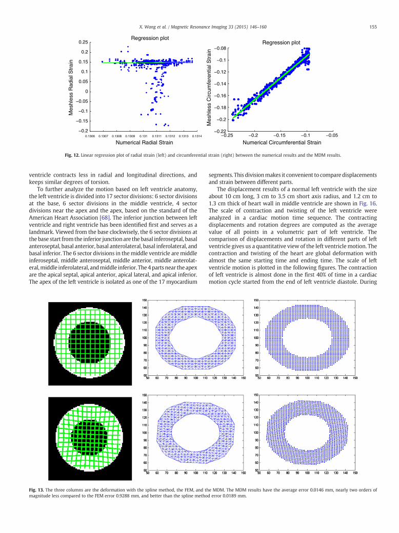
The estimation of circumferential and radial strain is evaluatedwith regression plots. In Fig. 12, the circumferential strain has largermagnitudes near endocardium. The regression line fits the data verywell, with R2 equal to 0.695. The errors between the meshless modelresult and the ground truth have the average value−0.02. The radial

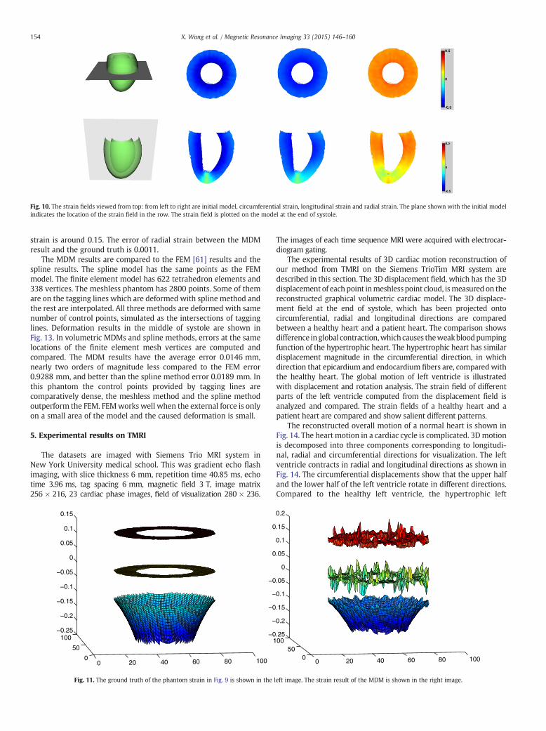
Fig. 10. The strain fields viewed from top: from left to right are initial model, circumferential strain, longitudinal strain and radial strain. The plane shown with the initial modeindicates the location of the strain field in the row. The strain field is plotted on the model at the end of systole.

154 X. Wang et al. / Magnetic Resonance Imaging 33 (2015) 146–160

strain is around 0.15. The error of radial strain between the MDMresult and the ground truth is 0.0011.

The MDM results are compared to the FEM [61] results and thespline results. The spline model has the same points as the FEMmodel. The finite element model has 622 tetrahedron elements and338 vertices. The meshless phantom has 2800 points. Some of themare on the tagging lines which are deformed with spline method andthe rest are interpolated. All three methods are deformed with samenumber of control points, simulated as the intersections of tagginglines. Deformation results in the middle of systole are shown inFig. 13. In volumetric MDMs and spline methods, errors at the samelocations of the finite element mesh vertices are computed andcompared. The MDM results have the average error 0.0146 mm,nearly two orders of magnitude less compared to the FEM error0.9288 mm, and better than the spline method error 0.0189 mm. Inthis phantom the control points provided by tagging lines arecomparatively dense, the meshless method and the spline methodoutperform the FEM. FEMworks well when the external force is onlyon a small area of the model and the caused deformation is small.

5. Experimental results on TMRI

The datasets are imaged with Siemens Trio MRI system inNew York University medical school. This was gradient echo flashimaging, with slice thickness 6 mm, repetition time 40.85 ms, echotime 3.96 ms, tag spacing 6 mm, magnetic field 3 T, image matrix256 × 216, 23 cardiac phase images, field of visualization 280 × 236.

0 20 40 60 80 1000

50

100−0.25

−0.2

−0.15

−0.1

−0.05

0

0.05

0.1

0.15

0 20 40 60 80 100050

100−0.25

−0.2

−0.15

−0.1

−0.05

0

0.05

0.1

0.15

0.2

Fig. 11. The ground truth of the phantom strain in Fig. 9 is shown in the left image. The strain result of the MDM is shown in the right image.

l

The images of each time sequence MRI were acquired with electrocar-diogram gating.

The experimental results of 3D cardiac motion reconstruction ofour method from TMRI on the Siemens TrioTim MRI system aredescribed in this section. The 3D displacement field, which has the 3Ddisplacement of each point inmeshless point cloud, ismeasured on thereconstructed graphical volumetric cardiac model. The 3D displace-ment field at the end of systole, which has been projected ontocircumferential, radial and longitudinal directions are comparedbetween a healthy heart and a patient heart. The comparison showsdifference in global contraction,which causes theweakbloodpumpingfunction of the hypertrophic heart. The hypertrophic heart has similardisplacement magnitude in the circumferential direction, in whichdirection that epicardium and endocardium fibers are, comparedwiththe healthy heart. The global motion of left ventricle is illustratedwith displacement and rotation analysis. The strain field of differentparts of the left ventricle computed from the displacement field isanalyzed and compared. The strain fields of a healthy heart and apatient heart are compared and show salient different patterns.

The reconstructed overall motion of a normal heart is shown inFig. 14. The heart motion in a cardiac cycle is complicated. 3Dmotionis decomposed into three components corresponding to longitudi-nal, radial and circumferential directions for visualization. The leftventricle contracts in radial and longitudinal directions as shown inFig. 14. The circumferential displacements show that the upper halfand the lower half of the left ventricle rotate in different directions.Compared to the healthy left ventricle, the hypertrophic left

0.1306 0.1307 0.1308 0.1309 0.131 0.1311 0.1312 0.1313 0.1314

−0.2

−0.15

−0.1

−0.05

0

0.05

0.1

0.15

0.2

0.25

Numerical Radial Strain

Mes

hles

s R

adia

l Str

ain

Regression plot

−0.25 −0.2 −0.15 −0.1 −0.05−0.22

−0.2

−0.18

−0.16

−0.14

−0.12

−0.1

−0.08

Numerical Circumferential Strain

Mes

hles

s C

ircum

fere

ntia

l Str

ain

Regression plot

Fig. 12. Linear regression plot of radial strain (left) and circumferential strain (right) between the numerical results and the MDM results.

155X. Wang et al. / Magnetic Resonance Imaging 33 (2015) 146–160

ventricle contracts less in radial and longitudinal directions, andkeeps similar degrees of torsion.

To further analyze the motion based on left ventricle anatomy,the left ventricle is divided into 17 sector divisions: 6 sector divisionsat the base, 6 sector divisions in the middle ventricle, 4 sectordivisions near the apex and the apex, based on the standard of theAmerican Heart Association [68]. The inferior junction between leftventricle and right ventricle has been identified first and serves as alandmark. Viewed from the base clockwisely, the 6 sector divisions atthe base start fromthe inferior junction are the basal inferoseptal, basalanteroseptal, basal anterior, basal anterolateral, basal inferolateral, andbasal inferior. The 6 sector divisions in themiddle ventricle aremiddleinferoseptal, middle anteroseptal, middle anterior, middle anterolat-eral,middle inferolateral, andmiddle inferior. The4parts near theapexare the apical septal, apical anterior, apical lateral, and apical inferior.The apex of the left ventricle is isolated as one of the 17 myocardium

Fig. 13. The three columns are the deformation with the spline method, the FEM, and the MDM. The MDM results have the average error 0.0146 mm, nearly two orders omagnitude less compared to the FEM error 0.9288 mm, and better than the spline method error 0.0189 mm.

segments. This divisionmakes it convenient to compare displacementsand strain between different parts.

The displacement results of a normal left ventricle with the sizeabout 10 cm long, 3 cm to 3.5 cm short axis radius, and 1.2 cm to1.3 cm thick of heart wall in middle ventricle are shown in Fig. 16.The scale of contraction and twisting of the left ventricle wereanalyzed in a cardiac motion time sequence. The contractingdisplacements and rotation degrees are computed as the averagevalue of all points in a volumetric part of left ventricle. Thecomparison of displacements and rotation in different parts of leftventricle gives us a quantitative view of the left ventricle motion. Thecontraction and twisting of the heart are global deformation withalmost the same starting time and ending time. The scale of leftventricle motion is plotted in the following figures. The contractionof left ventricle is almost done in the first 40% of time in a cardiacmotion cycle started from the end of left ventricle diastole. During

f

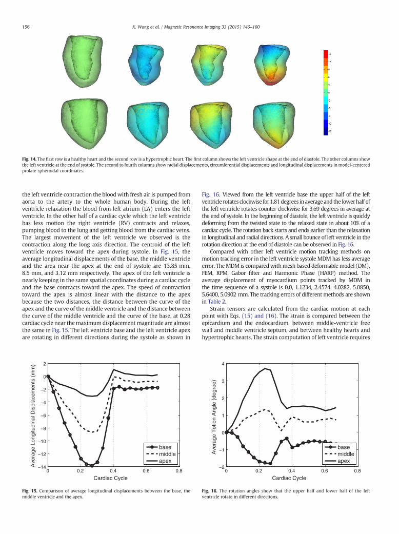
Fig. 14. The first row is a healthy heart and the second row is a hypertrophic heart. The first column shows the left ventricle shape at the end of diastole. The other columns showthe left ventricle at the end of systole. The second to fourth columns show radial displacements, circumferential displacements and longitudinal displacements in model-centeredprolate spheroidal coordinates.

156 X. Wang et al. / Magnetic Resonance Imaging 33 (2015) 146–160

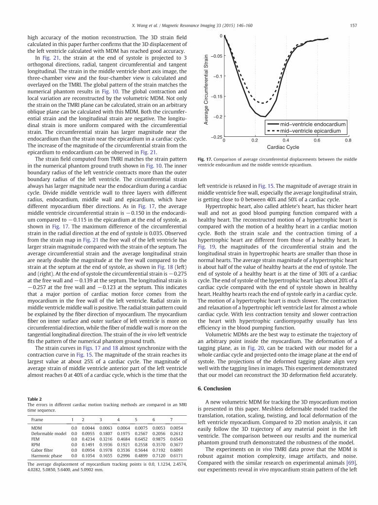
the left ventricle contraction the bloodwith fresh air is pumped fromaorta to the artery to the whole human body. During the leftventricle relaxation the blood from left atrium (LA) enters the leftventricle. In the other half of a cardiac cycle which the left ventriclehas less motion the right ventricle (RV) contracts and relaxes,pumping blood to the lung and getting blood from the cardiac veins.The largest movement of the left ventricle we observed is thecontraction along the long axis direction. The centroid of the leftventricle moves toward the apex during systole. In Fig. 15, theaverage longitudinal displacements of the base, the middle ventricleand the area near the apex at the end of systole are 13.85 mm,8.5 mm, and 3.12 mm respectively. The apex of the left ventricle isnearly keeping in the same spatial coordinates during a cardiac cycleand the base contracts toward the apex. The speed of contractiontoward the apex is almost linear with the distance to the apexbecause the two distances, the distance between the curve of theapex and the curve of the middle ventricle and the distance betweenthe curve of the middle ventricle and the curve of the base, at 0.28cardiac cycle near themaximumdisplacement magnitude are almostthe same in Fig. 15. The left ventricle base and the left ventricle apexare rotating in different directions during the systole as shown in

0 0.2 0.4 0.6 0.8−14

−12

−10

−8

−6

−4

−2

0

2

Cardiac Cycle

Ave

rage

Lon

gitu

dina

l Dis

plac

emen

ts (

mm

)

basemiddleapex

ig. 15. Comparison of average longitudinal displacements between the base, the

0 0.2 0.4 0.6 0.8−2

−1

0

1

2

3

4

Cardiac Cycle

Ave

rage

Tot

ion

Ang

le (

degr

ee)

basemiddleapex

Fig. 16. The rotation angles show that the upper half and lower half of the lef

F middle ventricle and the apex. ventricle rotate in different directions.

Fig. 16. Viewed from the left ventricle base the upper half of the leftventricle rotates clockwise for1.81degrees inaverageandthe lowerhalf ofthe left ventricle rotates counter clockwise for 3.69 degrees in average atthe end of systole. In the beginning of diastole, the left ventricle is quicklydeforming from the twisted state to the relaxed state in about 10% of acardiac cycle. The rotation back starts and ends earlier than the relaxationin longitudinal and radial directions. A small bounce of left ventricle in therotation direction at the end of diastole can be observed in Fig. 16.

Compared with other left ventricle motion tracking methods onmotion tracking error in the left ventricle systole MDM has less averageerror. TheMDM is comparedwithmesh based deformablemodel (DM),FEM, RPM, Gabor filter and Harmonic Phase (HARP) method. Theaverage displacement of myocardium points tracked by MDM inthe time sequence of a systole is 0.0, 1.1234, 2.4574, 4.0282, 5.0850,5.6400, 5.0902 mm. The tracking errors of different methods are shownin Table 2.

Strain tensors are calculated from the cardiac motion at eachpoint with Eqs. (15) and (16). The strain is compared between theepicardium and the endocardium, between middle-ventricle freewall and middle ventricle septum, and between healthy hearts andhypertrophic hearts. The strain computation of left ventricle requires

t

0 0.2 0.4 0.6 0.8−0.25

−0.2

−0.15

−0.1

−0.05

0

Cardiac Cycle

Ave

rage

Circ

umfe

rent

ial S

trai

n

mid−ventricle endocardiummid−ventricle epicardium

Fig. 17. Comparison of average circumferential displacements between the middleventricle endocardium and the middle ventricle epicardium.

157X. Wang et al. / Magnetic Resonance Imaging 33 (2015) 146–160

high accuracy of the motion reconstruction. The 3D strain fieldcalculated in this paper further confirms that the 3D displacement ofthe left ventricle calculated with MDM has reached good accuracy.

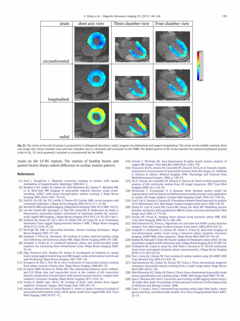
In Fig. 21, the strain at the end of systole is projected to 3orthogonal directions, radial, tangent circumferential and tangentlongitudinal. The strain in the middle ventricle short axis image, thethree-chamber view and the four-chamber view is calculated andoverlayed on the TMRI. The global pattern of the strain matches thenumerical phantom results in Fig. 10. The global contraction andlocal variation are reconstructed by the volumetric MDM. Not onlythe strain on the TMRI plane can be calculated, strain on an arbitraryoblique plane can be calculated with this MDM. Both the circumfer-ential strain and the longitudinal strain are negative. The longitu-dinal strain is more uniform compared with the circumferentialstrain. The circumferential strain has larger magnitude near theendocardium than the strain near the epicardium in a cardiac cycle.The increase of the magnitude of the circumferential strain from theepicardium to endocardium can be observed in Fig. 21.

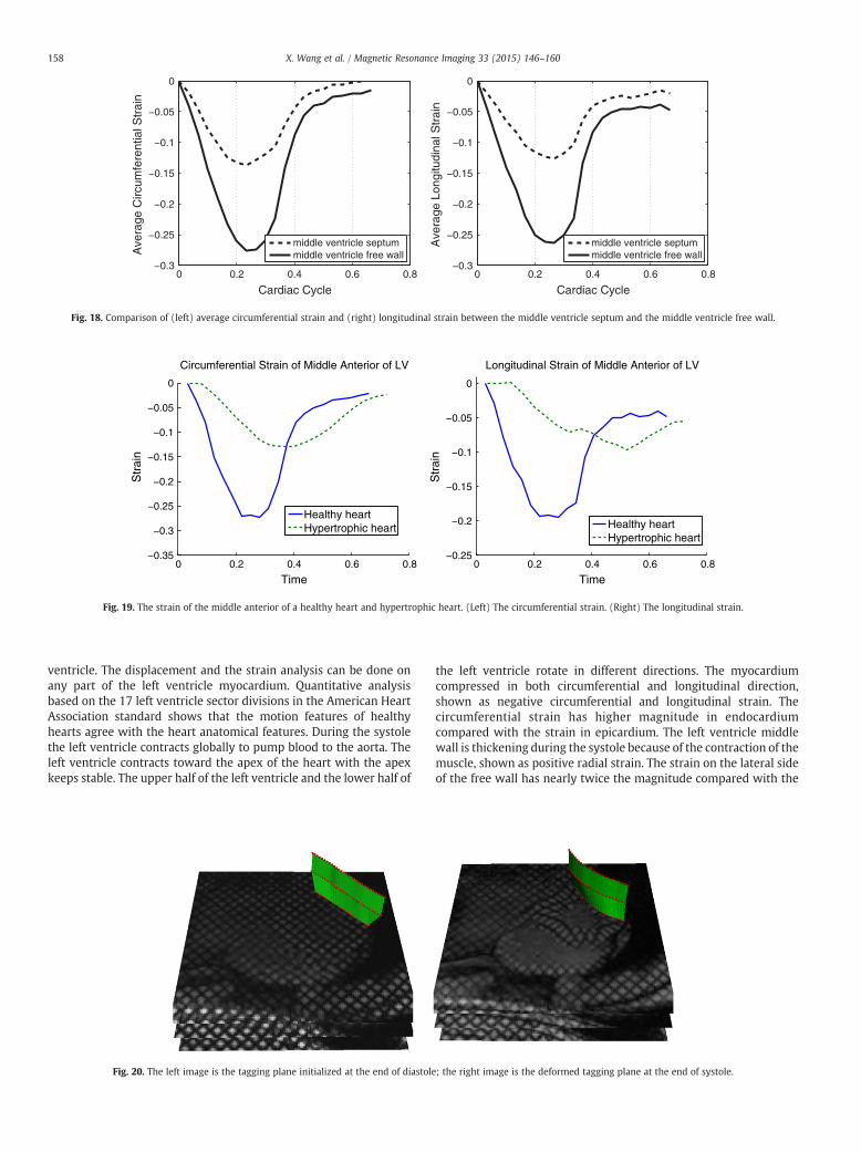
The strain field computed from TMRI matches the strain patternin the numerical phantom ground truth shown in Fig. 10. The innerboundary radius of the left ventricle contracts more than the outerboundary radius of the left ventricle. The circumferential strainalways has larger magnitude near the endocardium during a cardiaccycle. Divide middle ventricle wall to three layers with differentradius, endocardium, middle wall and epicardium, which havedifferent myocardium fiber directions. As in Fig. 17, the averagemiddle ventricle circumferential strain is −0.150 in the endocardi-um compared to −0.115 in the epicardium at the end of systole, asshown in Fig. 17. The maximum difference of the circumferentialstrain in the radial direction at the end of systole is 0.035. Observedfrom the strain map in Fig. 21 the free wall of the left ventricle haslarger strain magnitude compared with the strain of the septum. Theaverage circumferential strain and the average longitudinal strainare nearly double the magnitude at the free wall compared to thestrain at the septum at the end of systole, as shown in Fig. 18 (left)and (right). At the end of systole the circumferential strain is−0.275at the free wall and−0.139 at the septum. The longitudinal strain is−0.257 at the free wall and −0.123 at the septum. This indicatesthat a major portion of cardiac motion force comes from themyocardium in the free wall of the left ventricle. Radial strain inmiddle ventriclemiddlewall is positive. The radial strain pattern couldbe explained by the fiber direction of myocardium. The myocardiumfiber on inner surface and outer surface of left ventricle is more oncircumferential direction, while the fiber ofmiddle wall is more on thetangential longitudinal direction. The strain of the in vivo left ventriclefits the pattern of the numerical phantom ground truth.

The strain curves in Figs. 17 and 18 almost synchronize with thecontraction curve in Fig. 15. The magnitude of the strain reaches itslargest value at about 25% of a cardiac cycle. The magnitude ofaverage strain of middle ventricle anterior part of the left ventriclealmost reaches 0 at 40% of a cardiac cycle, which is the time that the

Table 2The errors in different cardiac motion tracking methods are compared in an MRtime sequence.

Frame 1 2 3 4 5 6 7

MDM 0.0 0.0044 0.0063 0.0064 0.0075 0.0053 0.0054Deformable model 0.0 0.0955 0.1807 0.1975 0.2567 0.2056 0.2612FEM 0.0 0.4234 0.3216 0.4684 0.6452 0.9875 0.6543RPM 0.0 0.1491 0.1936 0.1921 0.2558 0.3570 0.3677Gabor filter 0.0 0.0954 0.1978 0.3536 0.5644 0.7192 0.6091Harmonic phase 0.0 0.1054 0.1655 0.2996 0.4899 0.7120 0.6171

The average displacement of myocardium tracking points is 0.0, 1.1234, 2.45744.0282, 5.0850, 5.6400, and 5.0902 mm.

I

,

left ventricle is relaxed in Fig. 15. The magnitude of average strain inmiddle ventricle free wall, especially the average longitudinal strain,is getting close to 0 between 40% and 50% of a cardiac cycle.

Hypertrophic heart, also called athlete's heart, has thicker heartwall and not as good blood pumping function compared with ahealthy heart. The reconstructed motion of a hypertrophic heart iscompared with the motion of a healthy heart in a cardiac motioncycle. Both the strain scale and the contraction timing of ahypertrophic heart are different from those of a healthy heart. InFig. 19, the magnitudes of the circumferential strain and thelongitudinal strain in hypertrophic hearts are smaller than those innormal hearts. The average strain magnitude of a hypertrophic heartis about half of the value of healthy hearts at the end of systole. Theend of systole of a healthy heart is at the time of 30% of a cardiaccycle. The end of systole of the hypertrophic heart lags about 20% of acardiac cycle compared with the end of systole shown in healthyheart. Healthy hearts reach the end of systole early in a cardiac cycle.The motion of a hypertrophic heart is much slower. The contractionand relaxation of a hypertrophic left ventricle last for almost a wholecardiac cycle. With less contraction tensity and slower contractionthe heart with hypertrophic cardiomyopathy usually has lessefficiency in the blood pumping function.

Volumetric MDMs are the best way to estimate the trajectory ofan arbitrary point inside the myocardium. The deformation of atagging plane, as in Fig. 20, can be tracked with our model for awhole cardiac cycle and projected onto the image plane at the end ofsystole. The projections of the deformed tagging plane align verywell with the tagging lines in images. This experiment demonstratedthat our model can reconstruct the 3D deformation field accurately.

6. Conclusion

A new volumetric MDM for tracking the 3D myocardium motionis presented in this paper. Meshless deformable model tracked thetranslation, rotation, scaling, twisting, and local deformation of theleft ventricle myocardium. Compared to 2D motion analysis, it caneasily follow the 3D trajectory of any material point in the leftventricle. The comparison between our results and the numericalphantom ground truth demonstrated the robustness of the model.

The experiments on in vivo TMRI data prove that the MDM isrobust against motion complexity, image artifacts, and noise.Compared with the similar research on experimental animals [69],our experiments reveal in vivo myocardium strain pattern of the left

0 0.2 0.4 0.6 0.8−0.3

−0.25

−0.2

−0.15

−0.1

−0.05

0

Cardiac Cycle

Ave

rage

Circ

umfe

rent

ial S

trai

n

middle ventricle septummiddle ventricle free wall

0 0.2 0.4 0.6 0.8−0.3

−0.25

−0.2

−0.15

−0.1

−0.05

0

Cardiac Cycle

Ave

rage

Lon

gitu

dina

l Str

ain

middle ventricle septummiddle ventricle free wall

Fig. 18. Comparison of (left) average circumferential strain and (right) longitudinal strain between the middle ventricle septum and the middle ventricle free wall.

0 0.2 0.4 0.6 0.8−0.35

−0.3

−0.25

−0.2

−0.15

−0.1

−0.05

0

Time

Str

ain

Circumferential Strain of Middle Anterior of LV

Healthy heartHypertrophic heart

0 0.2 0.4 0.6 0.8−0.25

−0.2

−0.15

−0.1

−0.05

0

Time

Str

ain

Longitudinal Strain of Middle Anterior of LV

Healthy heartHypertrophic heart

Fig. 19. The strain of the middle anterior of a healthy heart and hypertrophic heart. (Left) The circumferential strain. (Right) The longitudinal strain.

158 X. Wang et al. / Magnetic Resonance Imaging 33 (2015) 146–160

ventricle. The displacement and the strain analysis can be done onany part of the left ventricle myocardium. Quantitative analysisbased on the 17 left ventricle sector divisions in the American HeartAssociation standard shows that the motion features of healthyhearts agree with the heart anatomical features. During the systolethe left ventricle contracts globally to pump blood to the aorta. Theleft ventricle contracts toward the apex of the heart with the apexkeeps stable. The upper half of the left ventricle and the lower half of

Fig. 20. The left image is the tagging plane initialized at the end of diastole; the right image is the deformed tagging plane at the end of systole.

the left ventricle rotate in different directions. The myocardiumcompressed in both circumferential and longitudinal direction,shown as negative circumferential and longitudinal strain. Thecircumferential strain has higher magnitude in endocardiumcompared with the strain in epicardium. The left ventricle middlewall is thickening during the systole because of the contraction of themuscle, shown as positive radial strain. The strain on the lateral sideof the free wall has nearly twice the magnitude compared with the

strain short axis view Three-chamber view Four-chamber view

circumferential

longitudinal

radial

Fig. 21. The strain at the end of systole is projected to 3 orthogonal directions: radial, tangent circumferential and tangent longitudinal. The strain on the middle ventricle shoraxis image slice, three-chamber view and four-chamber view is calculated and overlayed on the TMRI. The global pattern of the strain matches the numerical phantom groundtruth in Fig. 10. Local geometric variation is reconstructed by the MDM.

159X. Wang et al. / Magnetic Resonance Imaging 33 (2015) 146–160

strain on the LV-RV septum. The motion of healthy hearts andpatient hearts shows salient difference in cardiac motion pattern.

References

[1] Axel L, Dougherty L. Magnetic resonance imaging of motion with spatialmodulation of magnetization. Radiology 1989:841–5.

[2] Ibrahim E-SH, Stuber M, Fahmy AS, Abd-Elmoniem KZ, Sasano T, Abraham MR,et al. Real-time MR imaging of myocardial regional function using strain-encoding (SENC) with tissue through-plane motion tracking. J Magn ResonImaging 2007;26(6):1461–70 [12].

[3] Earls JP, Ho VB, Foo TK, Castillo E, Flamm SD. Cardiac MRI: recent progress andcontinued challenges. J Magn Reson Imaging 2002;16(2):111–27 [8].

[4] ReichekN.MRImyocardial tagging. JMagnReson Imaging1999;10(5):609–16 [11].[5] van der Paardt MP, Sprengers A, Zijta FM, Lamerichs R, Nederveen AJ, Stoker J.

Noninvasive automated motion assessment of intestinal motility by continu-ously tagged MR imaging. J Magn Reson Imaging 2014;39(1):9–16 2013 Apr 1.

[6] Tustison NJ, Awate SP, Cai J, Altes TA, Miller GW, de Lange EE, et al. Pulmonarykinematics from tagged hyperpolarized helium-3 MRI. J Magn Reson Imaging2010;31(5):1236–41 [5].

[7] McVeigh ER. MRI of myocardial function: motion tracking techniques. MagnReson Imaging 1995:137–50.

[8] Sampath S, Prince JL. Automatic 3D tracking of cardiac material markers usingslice-following and harmonic-phase MRI. Magn Reson Imaging 2006:197–208.

[9] Sampath S, Prince JL. A combined harmonic phase and strain-encoded pulsesequence for measuring three-dimensional strain. Magn Reson Imaging 2009:55–61.

[10] Olga Denisova JLW, Shapiro EP, Azhari H. Localization of ischemia in caninehearts using tagged rotated long axis MR images, endocardial surface stretch andwall thickening. Magn Reson Imaging 1997:1037–43.

[11] Drangova M, Zhu Y, Pelc NJ. In vitro verification of myocardial motion trackingfrom phase contrast velocity data. Magn Reson Imaging 1998:863–70.

[12] El-Sayed ABM, Ibrahim H, White RD. The relationship between aortic stiffnessand E/A filling ratio and myocardial strain in the context of left ventriculardiastolic dysfunction in heart failure with normal ejection fraction: insights frommagnetic resonance imaging. Magn Reson Imaging 2011:1222–34.

[13] Young A. Model tags: direct 3D tracking of heart wall motion from taggedmagnetic resonance images. Med Image Anal 1999:361–72.

[14] Huang J, Abendschein D, Davila-Roman V, Amini A. Spatio-temporal tracking ofmyocardial deformations with a 4D B-spline model from tagged MRI. IEEE TransMed Imaging 1999;18:957–72.

t

[15] Ozturk C, McVeigh ER. Four-dimensional B-spline based motion analysis oftagged MR images. Phys Med Biol 2000;46(6):1683–702.

[16] Duncan JS, Shi PC, Amimi AA, Constable RT, Dione D, Shi Q, et al. Towards reliable,noninvasive measurement of myocardial function from 4D images. In: HoffmanE, Acharya R, editors. Medical Imaging 1994: Physiology and Function fromMultidimensional Images; 1994. p. 149–61.

[17] Shi P, Sinusas AJ, Constable RT, Ritman E, Duncan JS. Point-tracked quantitativeanalysis of left ventricular motion from 3D image sequences. IEEE Trans MedImaging 2000;19(1):36–50.

[18] McInerney T, Terzopoulos D. A dynamic finite element surface model forsegmentation and tracking inmultidimensional medical imageswith applicationto cardiac 4D image analysis. Comput Med Imaging Graph 1995;19(1):69–83.

[19] Yan P, Lin N, Sinusas A, Duncan JS. A boundary element-based approach to analysisof LV deformation. Proc Med Image Comput Comput Assist Interv 2005:778–85.

[20] Wang VY, Lam H, Ennis DB, Cowan BR, Young AA, Nash MP. Modelling passivediastolic mechanics with quantitative MRI of cardiac structure and function. MedImage Anal 2009;13:773–84.

[21] Osman NF, Prince JL. Imaging heart motion using harmonic phase MRI. IEEETrans Med Imaging 2000;19(3):186–200.

[22] Abd-Elmoniem KZ, Prince J. Algorithms for real-time fast HARP cardiac functionanalysis. Proc Med Image Comput Comput Assist Interv 2003;2878:516–23.

[23] Sampath S, Derbyshire A, Osman NF, Atalar E, Prince JL. Real-time imaging oftwo-dimensional cardiac strain using a harmonic phase magnetic resonanceimaging (HARP-MRI) pulse sequence. Magn Reson Med 2003;50:154–63.

[24] ReyhanM, Natsuaki Y, Ennis DB. Fourier analysis of STimulated echoes (FAST) for thequantitative analysis of left ventricular twist. J Magn Reson Imaging 2012;35:587–93.

[25] Venkatesh BA, Gupta H, Lloyd SG, Dell ‘Italia L, Denney Jr TS. 3D left ventricularstrain from unwrapped harmonic phase measurements. J Magn Reson Imaging2010;31(4):854–62 [4].

[26] Pan L, Lima JAC, Osman NF. Fast tracking of cardiac motion using 3D-HARP. IEEETrans Biomed Eng 2005;52:1425–35.

[27] Abd-Elmoniem KZ, Stuber M, Osman NF, Prince J. Three-dimensional magneticresonance myocardial motion tracking from a single image plane. Magn ResonMed 2007;58:92–102.

[28] Abd-Elmoniem KZ, Stuber M, Prince J. Direct three-dimensional myocardial straintensor quantification and tracking using z HARP. Med Image Anal 2008:778–86.

[29] Qian Z, Metaxas DN, Axel L. Extraction and tracking of MRI tagging sheets using a3D Gabor filter bank. Proceedings of International Conference of the Engineeringin Medicine and Biology Society; 2006.

[30] Chen T, Chung S, Axel L. Automated tag tracking using Gabor filter banks, robustpoint matching, and deformable models. Proc Funct Imaging Model Heart 2007:22–31.

160 X. Wang et al. / Magnetic Resonance Imaging 33 (2015) 146–160

[31] Chen T, Wang X, Chung S, Metaxas D, Axel L. Automated 3D motion trackingusing Gabor filter bank, robust point matching, and deformable models. IEEETrans Med Imaging 2010;29:1–11.

[32] Park J, Metaxas D, Axel L. Deformable models with parameter functions forcardiac motion analysis. IEEE Transactions on Medical Imaging, 15 (3); 1996.p. 278–89.

[33] Park J, Metaxas D, Axel L. A finite element model for functional analysis of 4Dcardiac tagged MR images. Proceedings of Medical Image Computing andComputer-Assisted Intervention; 2003. p. 491–8.

[34] Metaxas DN, Terzopoulos D. Dynamic 3D models with local and globaldeformations: deformable superquadrics. IEEE Trans Pattern Anal Mach Intell1991;13(7):703–14.

[35] Haber E, Metaxas DN, Axel L. Motion analysis of the right ventricle from the MRIimages. Proc Med Image Comput Comput Assist Interv 1998:177–88.

[36] Haber I, Metaxas DN, Axel L. Three-dimensional motion reconstruction andanalysis of the right ventricle using taggedMRI. Med Image Anal 2000;4:335–55.

[37] Park K, Metaxas DN, Axel L. LV-RV shape modeling based on a blendedparameterized model. Proceedings of Medical Image Computing and Computer-Assisted Intervention. Springer-Verlag; 2002. p. 753–61.

[38] Park K, Metaxas DN, Axel L. A finite element model for functional analysis of 4Dcardiac-tagged MR images. Proceedings of Medical Image Computing andComputer-Assisted Intervention; 2003. p. 491–8.

[39] Belytschko T, Krongauz Y, Organ D, Fleming M, Krysl P. Meshless methods: anoverview and recent developments. Comput Methods Appl Mech Eng 1996:3–47.

[40] Muller M, Charypar D, Gross M. Particle-based fluid simulation for interactiveapplications. Proceedings of 2003 ACM SIGGRAPH; 2003. p. 154–9.

[41] Muller M, Keiser R, Nealen A, Pauly M, Gross M, Alexa M. Point based animationof elastic, plastic and melting objects. Proceedings of the 2004 ACM SIGGRAPH/Eurographics symposium on Computer animation; 2004. p. 141–51.

[42] Lancaster P, Salkauskas K. Surfaces generated by moving least squares methods.Math Comput 1981:141–58.

[43] Wang X, Chen T, Metaxas D, Axel L. Meshless deformable models for LV motionanalysis. Proceedings of Computer Vision and Pattern Recognition; 2008.

[44] Wang X, Chen T, Zhang S, Metaxas D, Axel L. LV motion and strain computationfrom TMRI based on meshless deformable models. Proc Med Image ComputComput Assist Interv 2008;1:636–44.

[45] Schneiders R, Oberschelp W, Kopp R, Becker M. New and effective remeshingscheme for the simulation of metal forming processes. Eng Comput 1992;8:163–76.

[46] Dannelongue H, Tanguy PA. Efficient data structures for adaptive remeshingwith the FEM. J Comput Phys 1990;91:94–109.

[47] Liu H, Shi P. Meshfree representation and computation: applications to cardiacmotion analysis. International Conference on Information Processing in MedicalImaging; 2003. p. 560–72.

[48] Liu H, Shi P. Meshfree particle method. Int Conf Comput Vis 2003:289–96.[49] Shi P, Liu H, Wong ALN, Wong KCL, Sinusas AJ. Meshfree cardiac motion analysis

using composite material model and total Lagrangian formulation. IEEE Int SympBiomed Imaging 2004:464–7.

[50] Wang L, Zhang H, Wong KCL, Liu H, Shi P. Electrocardiographic simulation onpersonalised heart-torso structures using coupled meshfree-BEM platform. Int JFunct Inform Pers Med 2009;2(2):175–200.

[51] Wong KCL, Wang L, Zhang L, Liu H, Shi P. Meshfree implementation of individualizedactive cardiac dynamics. Comput Med Imaging Graph 2010;34(1):91–103.

[52] Huang X, Metaxas D. Metamorphs: deformable shape and appearance models.IEEE Trans Pattern Anal Mach Intell 2008;30:1444–59.

[53] Qian Z,Metaxas DN, Axel L. Boosting and nonparametric based tracking of taggedMRI cardiac boundaries. Proc Med Image Comput Comput Assist Interv 2006:636–44.

[54] Montillo A, Metaxas DN, Axel L. Automated segmentation of the left and rightventricles in 4D cardiac SPAMM images. Med Image Comput Comput AssistInterv 2002:620–33.

[55] Montillo A, Metaxas DN, Axel L. Automated model-based segmentation of theleft and right ventricles in tagged cardiac mri. Med Image Comput Comput AssistInterv 2003:507–15.

[56] Axel L, Chen T, Mangli T. Dense myocardium deformation estimation for 2Dtagged MRI. Funct Imaging Model Heart 2005;3504:446–56.

[57] Chen T, Chung S, Axel L. 2D motion analysis of long axis cardiac tagged MRI. ProcMed Image Comput Comput Assist Interv 2007:469–76.

[58] Kerwin W, Prince J. Cardiac material markers from tagged MR images. MedImage Anal 1998;2:339–53.

[59] Lötjönen J, Reissman P-J, Magnin IE, Nenonen J, Katila T. A triangulation methodof an arbitrary point set for biomagnetic problems. IEEE Trans Magn 1998;34(4):2228–33.

[60] Schaerer J, Qian Z, Clarysse P, Metaxas D, Axel L, Magnin IE. Fast and automatedcreation of patient-specific 3D heart model from tagged MRI. MICCAI 2006workshop; 2006.

[61] Conway JB. A course in functional analysis. Graduate texts in mathematics. NewYork: Springer; 1990.

[62] Douglas RG. Onmajorization, factorization, and range inclusion and operators onHilbert space. Proc Am J Methmetical Soc 1966;17:413–5.

[63] Sorkine O, Lipman Y, Cohen-Or D, Alexa M, Rössl C, Seidel HP. Laplacian surfaceediting. Proceedings of the Eurographics/ACM SIGGRAPH Symposium onGeometry Processing. Eurographics Association; 2004. p. 179–88.

[64] Nealen A, Igarashi T, Sorkine O, Alexa M. Laplacian mesh opitimization.Proceedings of the 2006 ACM International Conference on Computer Graphicsand Interactive Techniques; 2006. p. 381–9.

[65] Zhang S, Wang X, Metaxas D, Chen T, Axel L. LV surface reconstruction fromsparse TMRI using Laplacian surface deformation and optimization. IEEE Int’lSymposium on Biomedical Imaging; 2009.

[66] Muller M, Heidelberger B, Teschner M, Gross M. Meshless deformation based onshape matching. Proceedings of the 32nd International Conference on ComputerGraphics and Interactive Techniques; 2005. p. 471–8.

[67] Teschner M, Heidelberger B, Müller M, Pomeranerts D, Gross M. Smoothedparticles: a new paradigm for animating highly deformable bodies. Proc VisModel Vis 2003:47–54.

[68] Cerqueira M, Weissman N, Dilsizian V, Jacobs A, Kaul S, Laskey W, et al.Standardized myocardial segmentation and nomenclature for tomographicimaging of the heart: a statement for healthcare professionals from the CardiacImaging Committee of the Council on Clinical Cardiology of the American HeartAssociation. J Am Heart Assoc 2002;105:539–42.

[69] Zhong J, Liu W, Yu X. Characterization of three-dimensional myocardialdeformation in the mouse heart: an MR tagging study. J Magn Reson Imaging2008;27(6):1263–70 [6].