Mesh Editing with Affine-Invariant Laplacian Coordinates

Technical Report HKUST-CS05-01

Hongbo Fu and Chiew-Lan Tai

Department of Computer ScienceHong Kong University of Science and Technology

Clear Water Bay, Kowloon, Hong KongE-mail: fuhb, taicl@cs.ust.hk

Abstract

Differential coordinates as an intrinsic surface representation capture geometric details of sur-face. However, differential coordinates alone cannot achieve desirable editing results, because theyare not affine invariant. In this paper, we present a novel method that makes the Laplacian coor-dinates completely affine-invariant during editing. For each vertex of a surface to be edited, wecompute the Laplacian coordinate and implicitly define a local affine transformation that is depen-dent on the unknown edited vertices. During editing, both the resulting surface and the implicitlocal affine transformations are solved simultaneously through a constrained optimization. The un-derlying mathematics of our method is a set of linear Partial Differential Equations (PDEs) with ageneralized boundary condition. The main computation involved comes from factorizing the result-ing sparse system of linear equations, which is performed only once. After that, back substitutionsare executed to interactively respond to user manipulations. We propose a new editing technique,called pose-independent merging, to demonstrate the advantages of the affine-invariant Laplaciancoordinates. In the the same framework, large-scale mesh deformation and pose-dependent meshmerging are also presented.

Keywords: Laplacian Coordinate, Affine-Invariant Transformation, Mesh Deformation, Pose-Independent Mesh Merging, Pose-Dependent Mesh Merging

1

=

(a) (b) (c)

=

Figure 1: An example of our pose-independent merging. The pose of a model means its position, orien-tation and scale. The task of this example is to merge the Mannequin head model to the Venus model.Before merging, the user only needs to specify the correspondence between the merging boundariesof these two models and does not need to adjust the poses of the models. In (a) and (b), the posesof the Venus model are the same, but the poses of the Mannequin head model are different. Ourpose-independent merging method creates the same result (c) for (a) and (b), given the same boundarycorrespondence. The two lines connecting the Mannequin head model and the Venus model indicatethe boundary correspondence.

1 Introduction

Modeling a complex surface from scratch is difficult and tedious. Mesh editing techniques aim tocreate new meshes from existing meshes, which are often obtained from a 3D scanner. Some desirableproperties of a mesh editing technique are detail-preservation, intuitiveness and interactivity. Designingan editing tool that satisfies all three properties is challenging.

This year, several important mesh editing techniques using differential representations have beenproposed [17, 23, 27]. The basic idea of these methods is to minimize the sum of squared differencesbetween the differential representations before and after editing, as the differential representations cap-ture geometric details of surface. The underlying mathematics of these methods is a system of linearPartial Differential Equations (PDEs) subject to a boundary condition. By editing the boundary condi-tion, the resulting surface is reconstructed through solving the linear system with the modified boundarycondition. All of these methods present intuitive and efficient ways to edit the boundary condition.

However, the differential representations in the above work are built in the global coordinate system.Thus they are only translation-invariant, but not scale-invariant or rotation-invariant [17]. To remedythis problem, the researchers proposed to either explicitly [17, 27] or implicitly [23] transform the dif-ferential representations prior to the reconstruction step. However, the proposed methods only partiallysolve the problem. None of the transformed differential representations is completely affine-invariant.In other words, if the user applies a global affine transformation, other than translation, to the boundarycondition, the details encoded by the differential coordinates are not transformed correspondingly.

In this paper, we propose a method that makes differential representations completely affine-invariant.The differential representation we shall use is the Laplacian coordinates [1, 23, 17], but our method iseasily extendable to other differential representations. To make the Laplacian coordinates invariant to

2

global affine transformations, we apply a local affine transformation to the Laplacian coordinate of eachvertex. The local affine transformation is determined by the original positions (known) of this vertexand its neighbors as well as the edited positions (unknown) of this vertex and its neighbors. Since thelocal affine transformations are dependent on the unknown positions of the edited vertices, our methodis classified as an implicit method. The major contributions of our work are as follows.

Affine-invariant Laplacian coordinates: We implicitly define a local affine transformation for theLaplacian coordinate of each vertex. During editing, the edited vertex positions and the local affinetransformations are simultaneously computed by solving a quadratic optimization problem subject toa generalized boundary condition and neighborhood coherence constraints. As both the Laplaciancoordinate and the local affine transformation associated with a vertex have local support dependenton this vertex and its neighbors, we only need to solve one sparse linear system. Similar to [27, 17,23, 24, 4], using the pre-computed LU factorization result of the sparse matrix, our method satisfies aninteractive rate even for editing regions with tens of thousands of vertices.

Large-scale mesh deformation: Based on the affine-invariant Laplacian coordinates, we present amesh deformation technique. During editing, the details encoded by the Laplacian coordinates are ap-propriately transformed by the implicit local affine transformations. Therefore, our approach is capableof performing large-scale deformation, which is difficult with existing Laplacian-based deformationtechniques [17, 23].

Pose-independent merging and pose-dependent merging: In most existing merging techniques,the first step the user needs to do is to adjust the poses of two meshes to be merged, including theirrelative positions, orientations and scales [23, 2, 19]. However, this is difficult for most novices, sincethey have to place an object in 3D space using 2D display and input devices [9]. We propose a newediting technique, called pose-independent merging, to successfully avoid this step. In our method, wefix the pose of one mesh, called the target mesh, and let the other mesh, called the source mesh, have afree pose. The task of the pose-independent merging is to simultaneously modify the pose of the sourcemesh and seamlessly merge the source mesh to the target mesh along two given merging boundaries.The only job for the user is to build the boundary correspondence. Figure 1 shows an example usingour pose-independent merging.

We unify pose-dependent merging into the same framework. In pose-dependent merging, besidesspecifying the boundary correspondence, the user needs to adjust the pose of the source mesh and tomark the regions in the source mesh to be fixed. This method is similar to the merging technique (calledtransplanting) in [23], but ours creates more satisfactory results due to the use of the affine-invariantLaplacian coordinates.

2 Related Work

Laplace operator: The most common form of encoding differential representations of surface meshesis the Laplace operator. It has been applied to many areas in geometric modeling and computer graph-ics, including mesh fairing [25, 8], surface parameterization [7], geometry compression [12, 22], meshmorphing [1], mesh editing [17, 23, 27, 4]. For mesh editing, the underlying theory can be formulatedusing the following linear system with the Dirichlet boundary condition:

∇2u = δF(u), u|∂Ω = u0|∂Ω, (1)

3

where ∇2 is the vector Laplacian, u is an unknown vector function, δ is a known vector, F is anunknown vector of linear functions applied to u, and u0 gives the values of u on the boundary ∂Ω.

Geometric details of the original meshes are encoded in δ . In [23, 17], it is obtained by applying theLaplace operator to each mesh vertex before editing (called the Laplacian coordinates). Yu et al. [27]define δ in another way: a gradient vector for each triangular face before editing is first computed andthen the divergence operator is applied. Essentially, these two detail-encoding methods are the same,as ∇2 = ∇ ·∇, where ∇ is the gradient operator and ∇· is the divergence operator.

Both the Laplacian coordinates and the gradient field are defined in the global coordinate system.Thus, they are neither rotation invariant nor scaling invariant. To address this problem, Sorkine etal. [23] apply an approximate rigid transformation represented by F(u) in Equation 1 to the Laplaciancoordinate of each vertex. Because the transformations are dependent on the unknown function u,theirs is an implicit method. In [17, 27], they explicitly modify δ (i.e. F(u) = 1). The resultingsystem is a set of Poisson equations. Our system is similar to the one in [23]. The main difference isthat in our method F(u) represents a set of local affine transformations instead of approximate rigidtransformations. Therefore, our method can handle large-angle rotations.

Botsch and Kobbelt [4] set δ to 0. Correspondingly, the system reduces to a set of Laplace equa-tions. Now the system carries no details. In other words, Equation 1 can only be applied to a surfacewithout any details. For the sake of detail-preserving editing, the authors integrate Equation 1 into amultiresolution modeling framework, i.e. Equation 1 is applied to a smooth surface at a low level ofdetail and the details are later added back to the modified smooth surface.

Mesh deformation: Free-form deformation (FFD) [20, 6, 18] is a powerful deformation tool incomputer animation and geometric modeling. FFD changes the shape of an object through a controllerby deforming the space dominated by the controller. According to the types of controllers, FFD can beclassified as lattice-based, surface-based, curve-based and point-based. One significant advantage ofthe FFD techniques is that they are independent of underlying model representations. However, FFDis mostly suitable for global deformations. Another type of global deformation is based on skeletons,which are regarded as a good shape description [16, 5].

To achieve both global deformations and local deformations, multiresolution-based schemes [28, 14,13, 10] have been proposed. A mesh is first decomposed into a sequence of levels of detail. Detailsas the difference between different levels are encoded with respect to local frames. Editing operationsare performed on coarse levels. After editing, details are added back to the modified coarse levels. Theuser can choose to apply editing operations on either coarse levels to obtain global deformations or finelevels to get local deformations. However, the number of vertices at coarse levels is usually still large.Hence, to deform surfaces at coarse levels, the user may have to resort to other deformation techniques(e.g. FFD).

This year, intrinsic differential representations have been adopted into the mesh deformation frame-works [17, 23, 27], because editing operations based on them are intuitive and detail-preserving. Theuser deforms a region of interest through manipulating a small number of handles, which may be com-posed of regions, curves or vertices. Due to the pre-computed factorization of linear systems, onlyexecuting a back substitution guarantees the efficiency of these methods. There have also been othertechniques related to intuitive mesh deformation [21, 24], in which deformations are defined by a smallnumber of user-marked control vertices. However, it is doubtful whether these methods can achieve asatisfactory interactive rate for large-scale meshes.

4

Mesh merging and surface pasting: Mesh merging and surface pasting are often used to createcompositions of existing models. Biermann et al. [3] proposed a cut-and-paste editing technique formultiresolution surfaces. It allows the user to decide the degree of details of the source mesh to bepasted onto the target mesh. A mesh fusion method presented in [11] forms smooth, connected surfacesfrom multiple parts. Levy [15] proposed a merging method by extrapolating parameterizations. All theabove methods involve parameterizing regions to be merged or pasted and thus they work only forregions homeomorphic to a disk.

Both Yu et al.[27] and Sorkine et al. [23] proposed merging techniques without 2D parameteriza-tion by connecting objects at their open boundaries. Both of them only require the topologies of themerging boundaries to be the same. In [23], the merging operation is performed by first filling the gapbetween the two merging boundaries and then mixing the details by surface reconstruction. The disad-vantage is that the two merging boundaries must have similar shapes. In [27], the two boundaries arefirst deformed to an intermediate boundary and then the deformation is propagated from the deformedboundaries to the interior of the two meshes. Therefore their method can handle merging of mesheswith different boundary shapes. Like these two merging methods, our merging methods do not requireany parameterization.

3 Affine-Invariant Laplacian Coordinates

In this section, we introduce our affine-invariant Laplacian coordinates. The Laplacian coordinates areobtained by applying the Laplace operator to each mesh vertex. In this paper, we use the same discreteLaplace operator D as that in [17, 23]:

δi = D(vi) = vi −1

|N(i)| ∑j∈N(i)

v j, (2)

where δi is the Laplacian coordinate for vertex vi and N(i) is the index set of the 1-ring neighboringvertices of vi. D is also known as an umbrella operator [25]. For highly irregular meshes, cotangentweights are often adopted instead of uniform weights [8].

3.1 Review of Laplacian-Based Editing

Nondegenerate Laplacian coordinates represent local details of surface: the direction and length ap-proximate the normal and curvature at each vertex, respectively. Therefore, the rationale of Laplacian-based mesh editing techniques is to minimize the sum of squared differences between the Laplaciancoordinates before and after editing [17, 23]. Here, it involves reconstructing the edited positions fromthe Laplacian coordinates. However, as the Laplace operator is applied to the absolute position ofeach vertex in the global coordinate system, the resulting Laplacian coordinates are only translation-invariant. Directly reconstructing the edited surface from the original Laplacian coordinates wouldcause undesirable artifacts. To solve this problem, Lipman et al. [17] proposed a two-step method.First, they reconstruct a rough surface using the original Laplacian coordinates and use the recon-structed surface to estimate a local rotation for each vertex. Second, the final surface is reconstructedfrom the Laplacian coordinates rectified by the local rotations. The method of [27] suffers from a sim-ilar problem (called Naıve Poisson editing) and also resorts to a two-step method: they propagate the

5

changes of orientations and scaling from the boundary condition to the entire gradient field, and thenperform a surface reconstruction with the modified gradient field.

Explicitly applying transformations to the Laplacian coordinates or gradient field works well formost editing cases. However, reconstructing the edited surface from the transformed differential rep-resentations is essentially a chicken-and-egg problem: on one hand, the resulting surface should bereconstructed from the modified Laplacian coordinates or gradient field; on the other hand, the trans-formations causing the modifications to the Laplacian coordinates or gradient field is dependent onthe resulting surface. Therefore, we believe that it is more appropriate to define local transformationsimplicitly rather than explicitly. Sorkine et al. [23] present an implicit method, which defines a localtransformation for the Laplacian coordinate at each vertex. However, the local transformation is onlyan approximate to a rigid transformation and isotropic scaling, which works well only for small anglesof rotations and cannot handle anisotropic scaling.

3.2 Local Affine Transformation

We propose an implicit method to address the problem. Our main task is to fit the resulting Laplaciancoordinates to the coordinates obtained by applying the implicit local affine transformations to theoriginal Laplacian coordinates.

We augment each Laplacian coordinate with a local affine transformation. It is applied to vi and its1-ring neighbors as follows:

Mivk +di = vk, k ∈ i∪N(i), (3)

where Mi is a 3× 3 matrix, di is the translation vector and vk is the unknown vertex. Together, Mi

and di define an affine transformation. We call the Laplacian coordinate augmented with the affinetransformation the affine-invariant Laplacian coordinate.

By eliminating di, we rewrite Equation 3 in matrix form as

MiVi = Vi (4)

whereVi = [vi −vi0 v j1 −vi0 v j2 −vi0 · · · v j|N(i)| −vi0 ]

Vi = [vi − vi0 v j1 − vi0 v j2 − vi0 · · · v j|N(i)| − vi0 ], j∗ ∈ N(i)

withvi0 =

1|N(i)| ∑

j∈N(i)v j and vi0 =

1|N(i)| ∑

j∈N(i)v j.

To get a least-squares solution for Mi in Equation 4, we consider the following equations

MiViVTi = ViVT

i . (5)

If ViVTi is invertible, we can directly derive Mi as

Mi = ViVTi (ViVT

i )−1. (6)

However, ViVTi is not always invertible. We check whether ViVT

i is invertible by testing whether itscorresponding condition number is greater than a given threshold (e.g, 5×10−5).

6

(a) (d)(b) (c) (e)

Figure 2: An example of handling the degenerate case of computing the local affine transformations.(a) A planar triangular mesh. The color of each mesh vertex is determined by the size of the Lapla-cian coordinate associated with this vertex. The different colors show that the mesh vertices are notuniformly distributed. (b) Selecting a region of interest to be deformed (blue) and a handle (green),through which the user controls the deformation effect. (c) As an initialization step, we add noise tothe degenerate vertices. In this example, all the vertices in the region of interest are degenerate. (d)Editing without removing the noise. (e) Editing with the noise removed.

The remaining task is to handle the case when ViVTi degenerates to a singular matrix. For simplicity,

we call the corresponding vertex vi a degenerate vertex. Now the rank of ViVTi is equal to 2, which

means that vi and its neighbors are coplanar. The idea is to move vi out of the plane. We let v′i denotethe modified vertex of vi. Since the directions of the nondegenerate Laplacian coordinates approximatethe normals, we place v′i in the normal direction at vi. The length of viv′i is set to a small randomnumber. Typically, we set

v′i = vi + scale ·ni, (7)

where ni is the unit normal vector at vi and scale = 0.2+0.1∗ random, random ∈ [0,1] (see an examplein Figure 2 (c)). With the modified vertex v′

i instead of vi, we compute Mi directly using Equation 6.Note that the Laplacian coordinate for vi must be recomputed using v′i. In addition, we compute theedited position v′i of v′i through the optimization instead of vi. Since the position of v′i is influencedby our deliberate noise (Figure 2 (d)), to get back the correct position of vi, we employ the followingequation

vi = Mi(vi −v′i)+ v′i. (8)

As any affine transformation preserves collinearity and ratios of distances, the final result with the noiseremoved is satisfactory (Figure 2 (e)).

Since we define a local affine transformation for each vertex and individual transformations obtainedfrom Equation 6 do not conform, we find an approximate solution. Specifically, we will minimize thefollowing error functional

EL =n

∑i=1

‖D(vi)−Miδi‖2, (9)

where n is the number of vertices in the region of interest. Since Mi is linearly dependent on theunknown vertices, EL is simply a quadratic function of the unknown vertices.

3.3 Boundary Condition and Neighborhood Coherence Constraints

Essentially, minimizing Equation 9 is equivalent to finding a least-squares solution of Equation 1. Ourmethod also needs the Dirichlet boundary condition. In our case, this type of boundary condition iscomposed of the positions of the vertices on the boundary curves, which define the region to be edited

7

and the handles to be manipulated (see the detailed user interaction in Section 4). Additionally, sincethe local affine transformations are linearly dependent on the unknown vertices, we need a generalizedboundary condition to constrain the minimization problem.

Similar to [27], we define a generalized boundary condition BC = (V,R,S), where V is the set ofmesh vertices on the Dirichlet boundary condition, R is a set of 3× 3 rotation matrices, and S is a setof scaling factors. There is a one-to-one correspondence among V , R and S. With R and S, we definean affine transformation for each vertex in V as a rotation transformation followed by a scaling trans-formation, denoted by SR. Before editing, the scaling factors and the rotation matrices are initializedto one and the identity matrix, respectively. We define a local Cartesian coordinate system at eachvertex in V , which is composed of its associated unit tangent vector along the boundary curve, unitnormal vector and the cross product of the previous two vectors. Then the rotation matrix is definedas the transformation from the original local Cartesian coordinate system to the edited local Cartesiancoordinate system. Each scaling factor is represented as the ratio of the distances between the vertexand the centroid of the boundary curve associated with the vertex after and before editing.

The definition of the generalized boundary condition in [27] contains a strength field, which is usedas a parameter to control how the transformations are propagated from the boundary condition to theregion to be edited. We do not need this field, since we implicitly define a local affine transformationfor each vertex of the boundary condition as well as the region to be edited.

Clearly, the local affine transformations are not independent of each other. Hence, to guarantee thesmoothness of the mesh after editing, the local affine transformations need to satisfy a set of neighbor-hood coherence constraints. A local affine transformation defined in Section 3.2 has a local support of1-ring neighbors. Therefore, our basic idea of neighborhood coherence constraints here is to partiallyoverlap the support domains of the affine transformations of neighboring vertices. With this idea, wefirst tried the following neighborhood coherence constraints:

(M(vi)−M(v j))(vi −v j) = 0, ∀i, ∀ j ∈ N(i). (10)

With the above constraints and the generalized boundary condition, minimizing the objective functionin Equation 9 indeed creates smooth results. However, since the support domain of a local affinetransformation (the 1-ring neighbors) also defines the Laplacian coordinate of a vertex, anisotropicscaling or shearing of the affine transformations will make the Laplacian coordinates deviate from thedirections of the respective normals. This causes undesirable editing artifacts. To solve this problem,we extend the support domain of each local affine transformation. Specifically, we define

ER =n

∑i=1

∑(i, j)∈SF

‖(M(vi)−M(v j))(vi −v j)‖2, (11)

where SF is a set of pairs of vertex indices: (i, j) ∈ SF if and only if two different faces containing vi

and v j respectively share one common edge. Now the support domain of each affine transformationis the 2-ring neighbors. We found that this definition has a stronger effect of preventing the deviationfrom the normal directions.

Now we define the following optimization problem for mesh editing:

arg min E(v1, . . . , vn) = EL +ER (12)

subject to vb j = u j, j ∈ 1 . . .s

M(vck) = Wk, k ∈ 1 . . .t

8

(a) (b) (c) (d) (e)

Figure 3: Basic operations for mesh deformation. (a) A horse: the original model with a region ofinterest (blue) and a handle (green) specified. To deform the region of interest, the user manipulates thehandle with 9 degrees of freedom, including translating (b), rotating (c), and scaling (d). (e) The regionof interest is deformed using a combination of the basic operations.

where u j is the position of a vertex with index b j on the boundary condition, Wk is the local affinetransformation at a vertex with index ck on the boundary condition, and s and t is the number of po-sition constraints and the number of transformation constraints, respectively. Usually we specify thepositions and the local affine transformations for the same set of boundary vertices (i.e. vb j= vck).Nevertheless, it is possible to allow some affine transformations to be specified, but their correspondingpositions to be free, and vice versa. This optimization problem is a standard constrained quadratic opti-mization problem. Therefore solving this problem is equivalent to solving a system of linear equations(see Section 6 for the implementation details).

4 Mesh Deformation

Since the objective function in our optimization problem is subject to the boundary condition, we caninfluence the solutions to this optimization problem by changing the boundary condition as in [17, 23,27, 4]. Specifically, we can change the generalized boundary condition (V,R,S) by adjusting the vertexpositions and local affine transformations of vertices in V . We develop a mesh deformation tool byproviding the user an intuitive interface to modify the generalized boundary condition.

Similar to [23, 4], our interface uses a set of handles to control the deformation results. The userspecifies a region of interest (ROI) bounded by a boundary curve, and defines at least one handle withinthe ROI (Figure 3 (a)). A handle may be a single vertex, a curve (open or closed), or a surface region.Then, the user deforms the ROI through the handles with 9 degrees of freedom, composed of the basicoperations including translating, rotating and scaling. For simplicity, we refer to the vertices of theboundary curve of the ROI and the vertices in the handles as constrained vertices. The constrainedvertices constitute the generalized boundary condition. The vertices within the ROI but not constrainedare called free vertices. The remaining vertices of the mesh is called fixed vertices. Each manipulationof a handle implies a global affine transformation. Correspondingly, the positions of the handle verticesand the associated local affine transformations are transformed by the global affine transformation.With the modified generalized boundary condition, the positions of the free vertices are reconstructedthrough the optimization.

Figure 3 shows the results of applying the basic deformation operations onto a horse model. Figure 4demonstrates that our deformation approach can easily handle the case with a large angle of rotation.This would be difficult with the deformation technique in [23].

9

Figure 4: Performing a large deformation on the Octopus model. Left: the original Octopus model.Right: the deformed model. Note that the circle stamps rotate with the attached neighboring surfaceafter deformation.

5 Mesh Merging

In mesh deformation, the boundary curve of the ROI is fixed and the handles are manipulated to modifythe boundary condition. Now we consider manipulating the boundary curve of the ROI and, if appli-cable, letting the handles be fixed. This leads to another application of our affine-invariant Laplaciancoordinates: mesh merging.

We present two merging techniques: pose-independent merging and pose-dependent merging. Here,the pose of an object means its stage, including its position, orientation and scale. Both these methodsmerge a source mesh to a target mesh along two designated boundaries. Our methods only require thetopologies of the source merging boundary and the target merging boundary to be the same and haveno restriction on the topologies of the source mesh and the target mesh. The pose of the target meshis always fixed. The pose of the source mesh is free in pose-independent merging and is user-specifiedin pose-dependent merging. The target mesh is never deformed. During the merging stage, only thetarget merging boundary is used as guidance to deform the source merging boundary. Consequently,the deformed source merging boundary provides the modified boundary condition to the optimizationproblem.

5.1 Pose-Independent Merging

Figure 5 demonstrates the advantage of using our affine-invariant Laplacian coordinates. In this exam-ple, we first compute the Laplacian coordinates for the region of interest (the entire model) shown inFigure 5 (a). Note that there is no handle specified within the ROI in this example. After applying aglobal affine transformation (rotation in Figure 5 (b) or scaling in Figure 5 (c)) to the boundary curve,the free vertices are reconstructed with the modified boundary condition by solving the optimizationproblem. The details are implicitly transformed by the local affine transformations. Our method guar-antees that all the local affine transformations are the same as the global affine transformation as ifthe global affine transformation is directly applied to the Laplacian coordinates. In Figure 6 of [27],a rotation or translation transformation is applied to the boundary condition, which gradually changes

10

(a) (b) (c)

Figure 5: If the boundary condition is transformed by a global affine transformation, the reconstructeddetails are transformed accordingly. (a) The original model with the entire mesh as the region of inter-est. (b) The reconstructed result after globally rotating the boundary condition. (c) The reconstructedresult after globally scaling the boundary condition.

the deformation from the boundary to the remaining part. The deformation results are dependent on theuser-specified strength field in the generalized boundary condition and the weighting scheme interpo-lating the boundary deformations. Since our optimization formulation in Equation 12 does not involvea strength field or weighting scheme, our pose-independent merging method provides a more automaticway.

To perform pose-independent merging, the user only needs to specify the correspondence betweenthe source merging boundary and the target merging boundary. We provide two ways to build thecorrespondence between two boundaries. The first one needs little user interaction. The user onlyspecifies the orientations (clockwise or counterclockwise) for the two boundaries and selects a startingvertex on each boundary. By parameterizing these two boundaries with the selected vertices as thestarting points, we can find the corresponding position on the target merging boundary for each vertexof the source merging boundary. The second one, similar to [27], needs the user to specify a set ofvertex correspondences. For the remaining vertices on the source merging boundary, the correspondingpositions on the target merging boundary are found through a curve parameterization. Since the poseof the source mesh is free, using the first method of only one vertex correspondence is sensitive toundulations in the boundaries. In this case, the user may adopt the second method to build a moreconfident boundary correspondence. In addition, the user should employ the second method if specificfeatures on the source and target meshes need to be matched.

After the boundary correspondence is determined, the Laplacian coordinates for the source mesh arecomputed and the local frames along the source merging boundary are built as described in Section 3.3.Then we modify the generalized boundary condition. The position of each vertex v of the sourcemerging boundary is set to its corresponding position v′ on the target merging boundary. The localframe at v′ is computed: the three axes are the unit tangent along the target merging boundary, the unitvertex normal and the cross product of the previous two vectors. The user may simultaneously rotateall the vertex normals along their corresponding tangents by the same angle to change the local framesdefined on the target merging boundary. The rotation matrix for v in the generalized boundary conditionis the rotation transformation from the local frame at v′ to the local frame at v. We define the scalingfactor for v as the ratio of the distance between v′ and the centroid of the target merging boundary tothe distance between v and the centroid of the source merging boundary. With the modified boundarycondition, the entire source mesh is reconstructed through the optimization.

To get a watertight seam, we remove the target merging boundary and its associated neighbors to

11

(a)

(b) (c)

Figure 6: The Headus skull model (b) is merged to the ears of the Stanford Bunny (a). The mergingboundaries of these two models have different shapes and have undulations. Note that the pose of theears is fixed and the pose of the skull is free.

obtain a new target merging boundary, and then fill the gap between it and the deformed source mergingboundary as follows. First, we find the closest vertex pair (u, v) between these two boundaries andconnect u and v. Next, we find a candidate from the neighboring vertices of these two vertices andconnect it to u or v. This process terminates once all the vertices on these two boundaries are visited.To improve the smoothness along the gap, an umbrella operator [25] is applied onto a band of facesencompassing the gap with several iterations.

Figure 1 shows the result of merging a source mesh in two different poses to a target mesh. Thisillustrates that, for the same boundary correspondence, our pose-independent merging produces thesame result. Figure 6 shows that our method also works well for merging boundaries with undulationsand different shapes. Figure 8 shows an example with multiple pairs of merging boundaries. In this ex-ample, the aim is to merge the centered CAD model to four cylinders. The CAD model is symmetrical,but the four cylinders have different positions and scales. Therefore, using the merging method in [23],the user would have great difficulty in adjusting the pose of the CAD model. Our pose-independentmerging method creates the same result, no matter what pose the CAD model is in before merging.This example also demonstrates that our merging method is applicable to meshes with non-zero genus.

5.2 Pose-Dependent Merging

In pose-independent merging, the entire source mesh is deformed and merged to the target mesh. Ifthe size of the source mesh is very large, its computation is expensive. Allowing only the region nearthe source merging boundary to be deformed can accelerate the merging progress. In addition, the usermay want to specify handles to fix specific features of the source mesh after merging. Such tasks canbe achieved using our pose-dependent merging.

12

(a) (b) (c) (d)

Figure 7: A comparison between pose-independent merging and pose-dependent merging when merg-ing the hind part of the Feline model (the source mesh) to the fore part of the Dinosaur model (the targetmesh). We use the same boundary correspondence for these two merging methods. The two handles(green) remain unchanged after merging.

Figure 8: A pose-independent merging example for multiple pairs of merging boundaries.

For pose-dependent merging, there are two things that need user interaction: the pose of the sourcemesh with respect to the pose of the target mesh and a set of handles on the source mesh. The remainingalgorithm is the same as the pose-independent merging one except for the following difference. In pose-dependent merging, we only modify the positions of the vertices of the source merging boundary andtheir scaling factors and keep their local frames unchanged. The deformed source merging boundaryand the fixed handles together provide the boundary condition to the optimization problem. This issimilar to the transplanting method in [23].

Figure 7 illustrates the difference between pose-independent merging and pose-dependent merging.Using pose-independent merging, the legs of the Feline model are not in harmony with the legs of theDinosaur model. When we fix the two feet of the Feline model, using pose-dependent merging, themerging result is more than acceptable. However, it is at the cost of adjusting the pose of the Felinemodel before merging.

13

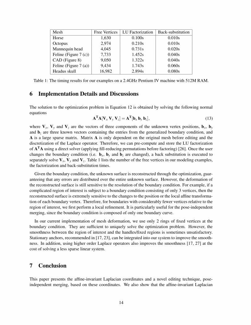
Mesh Free Vertices LU Factorization Back-substitutionHorse 1,630 0.100s 0.010sOctopus 2,974 0.210s 0.010sMannequin head 4,045 0.731s 0.020sFeline (Figure 7 (c)) 7,733 1.452s 0.040sCAD (Figure 8) 9,050 1.322s 0.040sFeline (Figure 7 (a)) 9,434 1.743s 0.060sHeadus skull 16,982 2.894s 0.080s

Table 1: The timing results for our examples on a 2.4GHz Pentium IV machine with 512M RAM.

6 Implementation Details and Discussions

The solution to the optimization problem in Equation 12 is obtained by solving the following normalequations

ATA[Vx Vy Vz] = AT[bx by bz], (13)

where Vx, Vy and Vz are the vectors of three components of the unknown vertex positions, bx, by

and bz are three known vectors containing the entries from the generalized boundary condition, andA is a large sparse matrix. Matrix A is only dependent on the original mesh before editing and thediscretization of the Laplace operator. Therefore, we can pre-compute and store the LU factorizationof ATA using a direct solver (applying fill-reducing permutations before factoring) [26]. Once the userchanges the boundary condition (i.e. bx, by and bz are changed), a back substitution is executed toseparately solve Vx, Vy and Vz. Table 1 lists the number of the free vertices in our modeling examples,the factorization and back-substitution times.

Given the boundary condition, the unknown surface is reconstructed through the optimization, guar-anteeing that any errors are distributed over the entire unknown surface. However, the deformation ofthe reconstructed surface is still sensitive to the resolution of the boundary condition. For example, if acomplicated region of interest is subject to a boundary condition consisting of only 3 vertices, then thereconstructed surface is extremely sensitive to the changes to the position or the local affine transforma-tion of each boundary vertex. Therefore, for boundaries with considerably fewer vertices relative to theregion of interest, we first perform a local refinement. It is particularly useful for the pose-independentmerging, since the boundary condition is composed of only one boundary curve.

In our current implementation of mesh deformation, we use only 2 rings of fixed vertices at theboundary condition. They are sufficient to uniquely solve the optimization problem. However, thesmoothness between the region of interest and the handles/fixed regions is sometimes unsatisfactory.Stationary anchors, recommended in [17, 23], can be integrated into our system to improve the smooth-ness. In addition, using higher order Laplace operators also improves the smoothness [17, 27] at thecost of solving a less sparse linear system.

7 Conclusion

This paper presents the affine-invariant Laplacian coordinates and a novel editing technique, pose-independent merging, based on these coordinates. We also show that the affine-invariant Laplacian

14

coordinates can be applied to pose-dependent merging and mesh deformation. All these editing tech-niques are automatically detail-preserving, due to the implicitly defined local affine transformation ateach vertex. The deformed or merged results are obtained by solving a constrained quadratic optimiza-tion problem at interactive rate.

For pose-dependent merging, we show that the user can choose to fix specific features during merg-ing. This capability can be extended to pose-independent merging. For each user-specified feature,we implicitly define an affine transformation that is applied to all the Laplacian coordinates associ-ated with this feature. In other words, in pose-independent merging, the feature is subject to an affinetransformation rather than completely fixed.

Acknowledgments The Octopus model and the horse model are courtesy of Mark Pauly and RobertW. Sumner, respectively. Other models are courtesy of Stanford University and 3D CAFE.

References

[1] Marc Alexa. Differential coordinates for local mesh morphing and deformation. The Visual Computer,19(2):105–114, 2003.

[2] Henning Biermann, Daniel Kristjansson, and Denis Zorin. Approximate boolean operations on free-formsolids. In Proceedings of ACM SIGGRAPH 2001, pages 185–194. ACM Press/ACM SIGGRAPH, 2001.

[3] Henning Biermann, Ioana Martin, Fausto Bernardini, and Denis Zorin. Cut-and-paste editing of multireso-lution surfaces. ACM Trans. Graph., 21(3):312–321, 2002.

[4] Mario Botsch and Leif Kobbelt. An intuitive framework for real-time freeform modeling. ACM Trans.Graph., 23(3):630–634, 2004.

[5] Steve Capell, Seth Green, Brian Curless, Tom Duchamp, and Zoran Popovic. Interactive skeleton-drivendynamic deformations. ACM Trans. Graph., 21(3):586–593, 2002.

[6] Sabine Coquillart. Extended free-form deformation: a sculpturing tool for 3d geometric modeling. InComputer Graphics (Proceedings of ACM SIGGRAPH 90), pages 187–196. ACM Press, 1990.

[7] Mathieu Desbrun, Mark Meyer, and Pierre Alliez. Intrinsic parameterizations of surface meshes. ComputerGraphics Forum, 21:209–218, 2002.

[8] Mathieu Desbrun, Mark Meyer, Peter Schroder, and Alan H. Barr. Implicit fairing of irregular meshes usingdiffusion and curvature flow. In Proceedings of ACM SIGGRAPH 99, pages 317–324. ACM Press/ACMSIGGRAPH, 1999.

[9] Thomas Funkhouser, Michael Kazhdan, Philip Shilane, Patrick Min, William Kiefer, Ayellet Tal, SzymonRusinkiewicz, and David Dobkin. Modeling by example. ACM Trans. Graph., 23(3):652–663, 2004.

[10] Igor Guskov, Wim Sweldens, and Peter Schroder. Multiresolution signal processing for meshes. In Pro-ceedings of ACM SIGGRAPH 99, pages 325–334. ACM Press/ACM SIGGRAPH, 1999.

[11] Takashi Kanai, Hiromasa Suzuki, Jun Mitani, and Fumihiko Kimura. Interactive mesh fusion based onlocal 3d metamorphosis. In Proceedings of the 1999 conference on Graphics interface ’99, pages 148–156.Morgan Kaufmann Publishers Inc., 1999.

[12] Zachi Karni and Craig Gotsman. Spectral compression of mesh geometry. In Proceedings of ACM SIG-GRAPH 2000, pages 279–286. ACM Press/ACM SIGGRAPH, 2000.

[13] Leif Kobbelt, Swen Campagna, Jens Vorsatz, and Hans-Peter Seidel. Interactive multi-resolution mod-eling on arbitrary meshes. In Proceedings of ACM SIGGRAPH 98, pages 105–114. ACM Press/ACMSIGGRAPH, 1998.

15

[14] Leif Kobbelt, Jens Vorsatz, and Hans-Peter Seidel. Multiresolution hierarchies on unstructured trianglemeshes. Comput. Geom. Theory Appl., 14(1-3):5–24, 1999.

[15] Bruno Levy. Dual domain extrapolation. ACM Trans. Graph., 22(3):364–369, 2003.

[16] J. P. Lewis, Matt Cordner, and Nickson Fong. Pose space deformation: a unified approach to shape interpo-lation and skeleton-driven deformation. In Proceedings of ACM SIGGRAPH 2000, pages 165–172. ACMPress/ACM SIGGRAPH, 2000.

[17] Yaron Lipman, Olga Sorkine, Daniel Cohen-Or, David Levin, Christian Rossl, and Hans-Peter Seidel.Differential coordinates for interactive mesh editing. In Proceedings of Shape Modeling International,pages 181–190. IEEE Computer Society Press, 2004.

[18] Ron MacCracken and Kenneth I. Joy. Free-form deformations with lattices of arbitrary topology. InProceedings of ACM SIGGRAPH 96, pages 181–188. ACM Press/ACM SIGGRAPH, 1996.

[19] Ken Museth, David E. Breen, Ross T. Whitaker, and Alan H. Barr. Level set surface editing operators.ACM Trans. Graph., 21(3):330–338, 2002.

[20] Thomas W. Sederberg and Scott R. Parry. Free-form deformation of solid geometric models. In ComputerGraphics (Proceedings of ACM SIGGRAPH 86), pages 151–160. ACM Press, 1986.

[21] Alla Sheffer and Vladislav Krayevoy. Shape preserving mesh deformation. SIGGRAPH 2004, sketches,2004. to appear.

[22] Olga Sorkine, Daniel Cohen-Or, and Sivan Toledo. High-pass quantization for mesh encoding. In Proceed-ings of the Eurographics/ACM SIGGRAPH symposium on Geometry processing, pages 42–51. Eurograph-ics Association, 2003.

[23] Olga Sorkine, Yaron Lipman, Daniel Cohen-Or, Marc Alexa, Christian Rossl, and Hans-Peter Seidel.Laplacian surface editing. In Proceedings of the Eurographics/ACM SIGGRAPH symposium on Geom-etry processing, pages 179–188. Eurographics Association, 2004.

[24] Robert W. Sumner and Jovan Popovic. Deformation transfer for triangle meshes. ACM Trans. Graph.,23(3):399–405, 2004.

[25] Gabriel Taubin. A signal processing approach to fair surface design. In Proceedings of ACM SIGGRAPH95, pages 351–358. ACM Press/ACM SIGGRAPH, 1995.

[26] Sivan Toledo. Taucs: A library of sparse linear solvers, version 2.2, 2003. Tel-Aviv University, Availableonline at http://www.tau.ac.il/ stoledo/taucs/.

[27] Yizhou Yu, Kun Zhou, Dong Xu, Xiaohan Shi, Hujun Bao, Baining Guo, and Heung-Yeung Shum. Meshediting with poisson-based gradient field manipulation. ACM Trans. Graph., 23(3):644–651, 2004.

[28] Denis Zorin, Peter Schroder, and Wim Sweldens. Interactive multiresolution mesh editing. In Proceedingsof ACM SIGGRAPH 97, pages 259–268. ACM Press/ACM SIGGRAPH, 1997.

16