HAL Id: tel-00338771https://tel.archives-ouvertes.fr/tel-00338771

Submitted on 14 Nov 2008

HAL is a multi-disciplinary open accessarchive for the deposit and dissemination of sci-entific research documents, whether they are pub-lished or not. The documents may come fromteaching and research institutions in France orabroad, or from public or private research centers.

L’archive ouverte pluridisciplinaire HAL, estdestinée au dépôt et à la diffusion de documentsscientifiques de niveau recherche, publiés ou non,émanant des établissements d’enseignement et derecherche français ou étrangers, des laboratoirespublics ou privés.

Mesh Compression from GeometryThomas Lewiner

To cite this version:Thomas Lewiner. Mesh Compression from Geometry. Computer Science [cs]. Université Pierre etMarie Curie - Paris VI, 2005. English. <tel-00338771>

Ecole Doctorale : E.D.I.T.E.

THESE

pour obtenir le titre de

Docteur en Sciencesde l’Universite Pierre et Marie Curie (Paris VI)

Mention: Informatique

presentee par

Thomas LEWINER

Compression de Maillages a partir de la Geometrie

(Mesh Compression from Geometry)

These dirigee par Jean–Daniel BOISSONNAT

preparee a l’INRIA Sophia Antipolis au sein du Projet Geometrica

et soutenue le 16, Decembre 2005

devant le jury compose de :

J.–D. Boissonnat INRIA — Sophia Antipolis DirecteurJ. Rossignac Georgia Tech — Atlanta RapporteurD. Cohen–Or Tel Aviv University RapporteurP. Frey UPMC — Paris PresidentH. Lopes PUC — Rio de Janeiro ExaminateurF. Schmitt ENST — Paris ExaminateurO. Devillers INRIA — Sophia Antipolis ExaminateurF. Lazarus INPG — Grenoble Examinateur

All rights reserved.

Thomas Lewiner

graduated from the Ecole Polytechnique (Paris, France) inAlgebra and Computer Science, and in Theoretical Phy-sics. He then specialized at the Ecole Superieure desTelecommunications (Paris, France) in Signal and Image Pro-cessing, and in Project Management, while working for Inven-tel in wireless telecommunication systems based on BlueToothtechnology. He then obtained a Master degree at the PontifıciaUniversidade Catolica do Rio de Janeiro in computational to-pology, and actively participated to the Mathematical depart-ment’s work for Petrobras.

Bibliographic descriptionLewiner, Thomas

Mesh Compression from Geometry / Thomas Lewiner;adviser: Jean–Daniel Boissonnat.— Paris : UniversitePierre et Marie Curie (Paris VI), 2005 [Projet Geometrica,INRIA Sophia Antipolis].—

1 vol. (159 p.) : ill. ; 29,7 cm.—

PhD Thesis.— Universite Pierre et Marie Curie (Pa-ris VI) : prepared at the Projet Geometrica, INRIA SophiaAntipolis.—

Bibliography included.—

1. Computer Science – Thesis. 2. Mesh Compression.3. Geometry–Driven Compression. 4. Level sets. 5. Isosur-faces. 6. Isosurface compression. 7. Computational Geo-metry. 8. Solid Modelling. 9. Data Compaction. I. Le-winer, Thomas. II. Boissonnat, Jean–Daniel. III. ProjetGeometrica, INRIA Sophia Antipolis. IV. E.D.I.T.E., Uni-versite Pierre et Marie Curie (Paris VI). V. Mesh Com-pression from Geometry.

Thomas Lewiner

Mesh Compression from Geometry

Thesis prepared at the Projet Geometrica, INRIA SophiaAntipolis as partial fulfilment of the requirements for thedegree of Doctor in Philosophy in Computer Science of theUniversite Pierre et Marie Curie (Paris VI), and submitted tothe following commission:

J.–D. Boissonnat (Adviser)INRIA — Sophia Antipolis

J. Rossignac (Referee)Georgia Tech — Atlanta

D. Cohen–Or (Referee)Tel Aviv University

P. Frey (President)UPMC — Paris

H. Lopes (Examinator)PUC — Rio de Janeiro

F. Schmitt (Examinator)ENST — Paris

O. Devillers (Examinator)INRIA — Sophia Antipolis

F. Lazarus (Examinator)INPG — Grenoble

Paris — 16, Decembre 2005

Acknowledgments

This is my second PhD redaction, and my tribute to the many people who

helped me remains. First of all, my father who motivated me for science and

always supported me, especially in difficult moments, my mother and my grand

mother who made me feel this wonderful familiar environment wherever I was.

I am also particularly grateful to my advisor Jean–Daniel for his support and

encouragements along these three years. He maintained a very open–minded

vision that allowed me to convey many ideas between France and Brazil, and

this has been very fruitful for my professional and personal formation. His

support has been relayed by the everyday work of Agnes and Creuza, the help

of Francis Schmitt in the defence organisation, of Pierre Deransart and Rachid

Deriche from the International Relations of the INRIA, the funding of the

Fondation de l’Ecole Polytechnique, and the access conceded by the Pontifıcia

Universidade Catolica do Rio de Janeiro. Moreover, I would like to thank

particularly Agnes, Marie–Pierre and Dominique for the help in preparing the

defence, the referees and the jury members for the exceptional attention they

manifested for this work.

This big team that welcomed my projects allowed a wide exchange of

point of views, with the practise of Helio, Pierre and Sinesio, the experience

of Jean–Daniel, Olivier, Luiz and Geovan, the lights of Marcos, Carlos and

David and the cooperation of my colleagues of both sides: Vinıcius, Wilson,

Marcos, Rener, Alex, Cynthia, Afonso, Jessica, Christina, Francisco, Fabiano,

Marcos and Marie, Luca, David, Marc, Steve, Philippe, Camille, Christophe,

Abdelkrim and Laurent. In particular, I would like to thank Vinıcius for his

great help in the use of his data structure, and Luiz and Helio for the starting

ideas of at least half of this work.

But the scientific help is not sufficient to achieve this work, and the

emotive support has been crucial for leading it. This constant energy along

these three years came from the presence of my grandmother during the

preparation of this work, the souvenir of Fanny and Simone, the eternal

support of my parents, the complicity of my sisters, brothers–in–law and of

Debora together with the tight friendship of my uncles, ants and cousins. I

also felt this warmness with my friends, and I am happy that this includes

my professors and colleagues, with Albane, JA, Anne–Laure, Juliana(s), Ana

Cristina, Silvana, Tania, Benjamin, Nicolas, David(s), Aurelien, Eric, Mathieu,

Sergio(s), Bernardo, . . .

Resume

Lewiner, Thomas ; Boissonnat, Jean–Daniel. Compres-sion de Maillages a partir de la Geometrie. Paris,2005. 159p. These de Doctorat — Universite Pierre etMarie Curie (Paris VI) : preparee au Projet Geometrica,INRIA Sophia Antipolis.

Les images ont envahi la plupart des publications et des communications

contemporaines. Cette expansion s’est acceleres avec le developpement de

methodes efficaces de compression specifiques d’images. Aujourd’hui, la

generation d’images s’appuie sur des objets multidimensionnels produits

a partir de dessins assistes par ordinateurs, de simulations physiques, de

representations de donnees ou de solutions de problemes d’optimisation.

Cette variete de sources motive la conception de schemas dedies de com-

pression adaptes a des classes specifiques de modeles. Ce travail presente

deux methodes de compression pour des modeles geometriques. La premiere

code des ensembles de niveau en dimension quelconque, de maniere directe

ou progressive, avec des taux de compression au niveau de l’etat de l’art

pour les petites dimensions. La seconde methode code des maillages de

n’importe quelle dimension ou topologie, meme sans etre purs ou variete,

plonges dans des espaces arbitraires. Les taux de compression pour les sur-

faces sont comparables aux methodes usuelles de compression de maillages

comme Edgebreaker.

Mots–ClefsCompression de Maillages. Compression orientee par la Geometrie.

Ensembles de Niveau. Isosurfaces. Compression d’Isosurfaces. Geometrie

Algorithmique. Modelage Geometrique. Compression de Donnees.

Abstract

Lewiner, Thomas ; Boissonnat, Jean–Daniel. MeshCompression from Geometry. Paris, 2005. 159p.PhD Thesis — Universite Pierre et Marie Curie(Paris VI) : prepared at the Projet Geometrica, INRIASophia Antipolis.

Images invaded most of contemporary publications and communications.

This expansion has accelerated with the development of efficient schemes

dedicated to image compression. Nowadays, the image creation process relies

on multidimensional objects generated from computer aided design, physical

simulations, data representation or optimisation problem solutions. This

variety of sources motivates the design of compression schemes adapted to

specific class of models. This work introduces two compression schemes for

geometrical models. The first one encodes level sets in any dimension, in a

direct or progressive manner, with both state of the art compression ratios

for low dimensions. The second one encodes meshes of any dimension and

topology, even non–pure or non–manifold models, embedded in arbitrary

space. The compression ratios for surfaces are comparable with famous mesh

compression methods such as the Edgebreaker.

KeywordsMesh Compression. Geometry–Driven Compression. Level sets. Iso-

surfaces. Isosurface compression. Computational Geometry. Solid Mod-

elling. Data Compaction.

Contents

I Introduction 11

II Encoding and Compression 19

II.1 Information Representation 19Coding 19Information Theory 20Levels of Information 21

II.2 Arithmetic Coding 22Arithmetic Coder 22Algorithms 23Statistical Modelling 25

II.3 Compression 27Compaction 28Direct Compression 28Progressive Compression 28

III Meshes and Geometry 29

III.1 Simplicial Complexes and Polytopes 29Simplicial Complexes 30Local Structure 31Pure Simplicial Complexes 32Simplicial Manifolds 32Polytopes 33

III.2 Combinatorial Operators 34Euler Operators 34Handle Operators 36Stellar Operators 38

III.3 Geometry and Discretisation 39Subdivision and Smoothing 40Delaunay Triangulation 41Multi–Triangulations 42

IV Connectivity–Driven Compression 47

IV.1 Principles 47Origins 52Primal or dual remainders 52Topological Singularities 54

IV.2 The Edgebreaker example 55CLERS encoding 56Fast decompression 57Topology encoding 58Compression algorithms 61

7 Contents

Decompression algorithms 61

IV.3 Performances 66Compression Rates 66Good and bad cases 67Extensions 69

V Level Set Compression 73

V.1 Level Set Extraction 75Simplicial Interpolation 76Geometry and Distortion Control 77Topology Control 79

V.2 Direct Encoding 81Localisation 82Uniform Encoding 83Adapted Encoding 84

V.3 Progressive Encoding 85Combinatorial Refinement 85Extrinsic Geometry Refinement 87Level Sets Extensions 88

V.4 Tuning and Results 88Prediction and Statistical Models 88Direct 90Progressive 90Extended applications 93

VI GEncode 97

VI.1 Purposes 97Focus on Geometrical Meshes 97Zero Cost for Reconstructible Meshes 98Independent Geometry Encoding 99

VI.2 GEncode schemes 102Advancing front compression 102Optimisations and Extensions 102Candidates selection 105

VI.3 Geometric Criteria 107Generic Formulation 107Ball–Pivoting and Delaunay–Based Reconstruction 108Parametric Criterion 110

VI.4 Results 112

VII Conclusions and Future Works 115

Resume en francais 117

Bibliography 145

Index 157

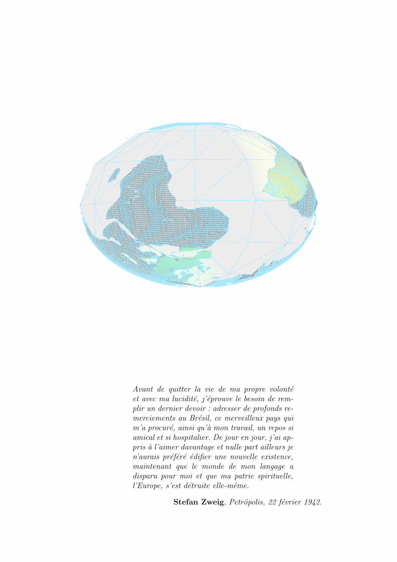
Avant de quitter la vie de ma propre volonteet avec ma lucidite, j’eprouve le besoin de rem-plir un dernier devoir : adresser de profonds re-merciements au Bresil, ce merveilleux pays quim’a procure, ainsi qu’a mon travail, un repos siamical et si hospitalier. De jour en jour, j’ai ap-pris a l’aimer davantage et nulle part ailleurs jen’aurais prefere edifier une nouvelle existence,maintenant que le monde de mon langage adisparu pour moi et que ma patrie spirituelle,l’Europe, s’est detruite elle-meme.

Stefan Zweig, Petropolis, 22 fevrier 1942.

IIntroduction

Images surpassed the simple function of illustrations. In particular, artificialand digital images invaded most of published works, from commercial identi-fication to scientific explanation, together with the specific graphics industry.Technical advances created supports, formats and transmission protocols forthese images, and these contributed to this expansion. Among these, high qual-ity formats requiring low resources appeared with the development of generic,and then specific, compression schemes for images. More recently drew on thesustained trend to incorporate the third dimension into images, and this mo-tivates orienting the developments of compression towards higher dimensionalimages.

There exists a wide variety of images, from photographic material todrawings and artificial pictures. Similarly, higher dimensional models areproduced from many sources: The graphics industry designers draw three–dimensional objects by their contouring surface, using geometric primitives.The recent developments of radiology make intense use of three–dimensionalimages of the human body, and extract isosurfaces to represent organs andtissues. Geographic and geologic models of terrain and underground consistin surfaces in the multi–dimensional of physical measures. Engineering usuallygenerate finite elements solid meshes in similar multi–dimensional spaces tosupport physical simulations, while reverse engineering, archæological heritagepreservation and commercial marketing reconstruct real objects from scannedsamplings. In addition, other fields are adding new multi–dimensional mod-elling, such as data representation and optimisation, particularly for solvingfinancial problems.

Compression methods for three–dimensional models appeared mainly inthe mid 1990’s with [Deering 1995] and developed quickly since then. Thisevolution turned out to be a technical necessity, since the size and complex-ity of the typical models used in practical applications increases rapidly. Themost performing practical strategies for surfaces are based on the Edgebreakerof [Rossignac 1999] and the valence coding of [Touma and Gotsman 1998].These are classified as connectivity–driven mesh compression, since the prox-imity of triangles guides the sequence of the surface vertices to be encoded.More recently, dual approaches proposed to guide the encoding of the triangleproximity by the geometry, such as done in [Gandoin and Devillers 2002].

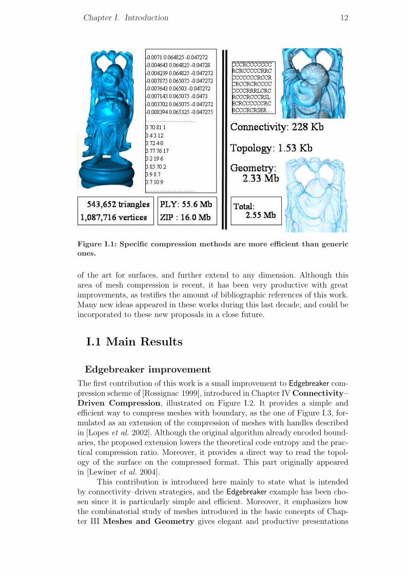
Actually, the diversity of images requires this multiplicity of compressionprograms, since specific algorithms usually perform better than generic one, ifthey are well adapted, as illustrated on Figure I.1. This work focuses on twonew geometry–driven compression methods that compare nicely to the state

Chapter I. Introduction 12

Figure I.1: Specific compression methods are more efficient than genericones.

of the art for surfaces, and further extend to any dimension. Although thisarea of mesh compression is recent, it has been very productive with greatimprovements, as testifies the amount of bibliographic references of this work.Many new ideas appeared in these works during this last decade, and could beincorporated to these new proposals in a close future.

I.1 Main Results

Edgebreaker improvement

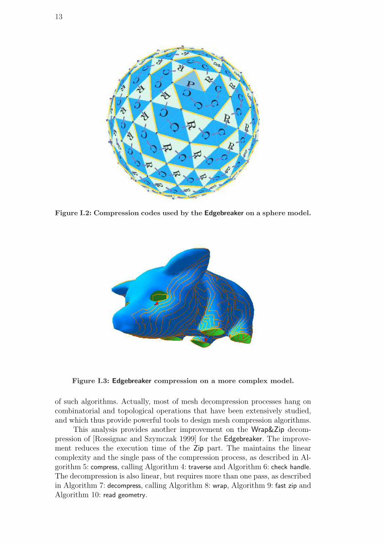
The first contribution of this work is a small improvement to Edgebreaker com-pression scheme of [Rossignac 1999], introduced in Chapter IV Connectivity–Driven Compression, illustrated on Figure I.2. It provides a simple andefficient way to compress meshes with boundary, as the one of Figure I.3, for-mulated as an extension of the compression of meshes with handles describedin [Lopes et al. 2002]. Although the original algorithm already encoded bound-aries, the proposed extension lowers the theoretical code entropy and the prac-tical compression ratio. Moreover, it provides a direct way to read the topol-ogy of the surface on the compressed format. This part originally appearedin [Lewiner et al. 2004].

This contribution is introduced here mainly to state what is intendedby connectivity–driven strategies, and the Edgebreaker example has been cho-sen since it is particularly simple and efficient. Moreover, it emphasizes howthe combinatorial study of meshes introduced in the basic concepts of Chap-ter III Meshes and Geometry gives elegant and productive presentations

13

Figure I.2: Compression codes used by the Edgebreaker on a sphere model.

Figure I.3: Edgebreaker compression on a more complex model.

of such algorithms. Actually, most of mesh decompression processes hang oncombinatorial and topological operations that have been extensively studied,and which thus provide powerful tools to design mesh compression algorithms.

This analysis provides another improvement on the Wrap&Zip decom-pression of [Rossignac and Szymczak 1999] for the Edgebreaker. The improve-ment reduces the execution time of the Zip part. The maintains the linearcomplexity and the single pass of the compression process, as described in Al-gorithm 5: compress, calling Algorithm 4: traverse and Algorithm 6: check handle.The decompression is also linear, but requires more than one pass, as describedin Algorithm 7: decompress, calling Algorithm 8: wrap, Algorithm 9: fast zip andAlgorithm 10: read geometry.

Chapter I. Introduction 14

Level sets direct and progressive compression

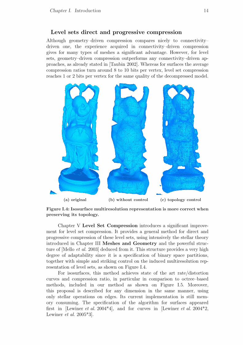
Although geometry–driven compression compares nicely to connectivity–driven one, the experience acquired in connectivity–driven compressiongives for many types of meshes a significant advantage. However, for levelsets, geometry–driven compression outperforms any connectivity–driven ap-proaches, as already stated in [Taubin 2002]. Whereas for surfaces the averagecompression ratios turn around 8 to 10 bits per vertex, level set compressionreaches 1 or 2 bits per vertex for the same quality of the decompressed model.

(a) original (b) without control (c) topology control

Figure I.4: Isosurface multiresolution representation is more correct whenpreserving its topology.

Chapter V Level Set Compression introduces a significant improve-ment for level set compression. It provides a general method for direct andprogressive compression of these level sets, using intensively the stellar theoryintroduced in Chapter III Meshes and Geometry and the powerful struc-ture of [Mello et al. 2003] deduced from it. This structure provides a very highdegree of adaptability since it is a specification of binary space partitions,together with simple and striking control on the induced multiresolution rep-resentation of level sets, as shown on Figure I.4.

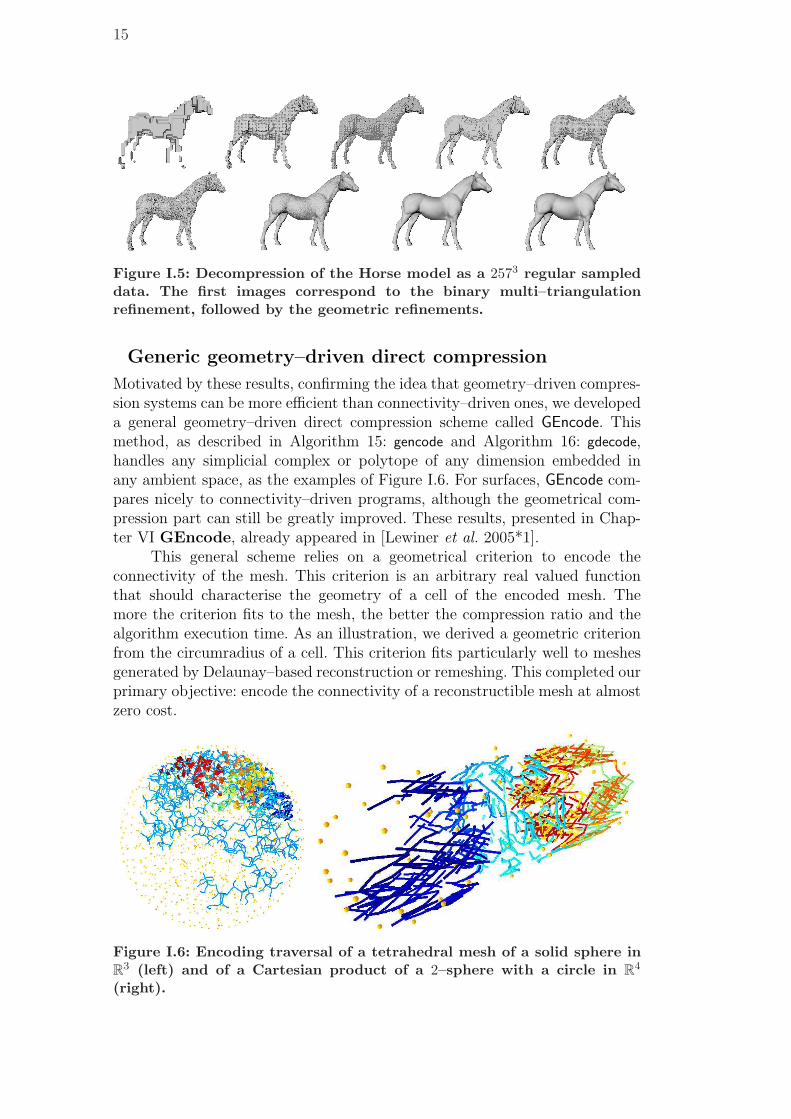
For isosurfaces, this method achieves state of the art rate/distortioncurves and compression ratio, in particular in comparison to octree–basedmethods, included in our method as shown on Figure I.5. Moreover,this proposal is described for any dimension in the same manner, usingonly stellar operations on edges. Its current implementation is still mem-ory consuming. The specification of the algorithm for surfaces appearedfirst in [Lewiner et al. 2004*4], and for curves in [Lewiner et al. 2004*2,Lewiner et al. 2005*3].

15

Figure I.5: Decompression of the Horse model as a 2573 regular sampleddata. The first images correspond to the binary multi–triangulationrefinement, followed by the geometric refinements.

Generic geometry–driven direct compression

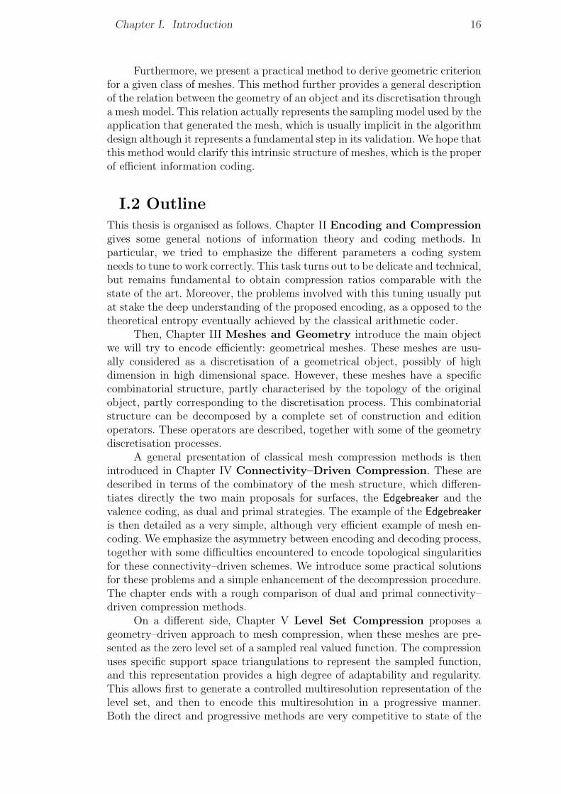
Motivated by these results, confirming the idea that geometry–driven compres-sion systems can be more efficient than connectivity–driven ones, we developeda general geometry–driven direct compression scheme called GEncode. Thismethod, as described in Algorithm 15: gencode and Algorithm 16: gdecode,handles any simplicial complex or polytope of any dimension embedded inany ambient space, as the examples of Figure I.6. For surfaces, GEncode com-pares nicely to connectivity–driven programs, although the geometrical com-pression part can still be greatly improved. These results, presented in Chap-ter VI GEncode, already appeared in [Lewiner et al. 2005*1].

This general scheme relies on a geometrical criterion to encode theconnectivity of the mesh. This criterion is an arbitrary real valued functionthat should characterise the geometry of a cell of the encoded mesh. Themore the criterion fits to the mesh, the better the compression ratio and thealgorithm execution time. As an illustration, we derived a geometric criterionfrom the circumradius of a cell. This criterion fits particularly well to meshesgenerated by Delaunay–based reconstruction or remeshing. This completed ourprimary objective: encode the connectivity of a reconstructible mesh at almostzero cost.

Figure I.6: Encoding traversal of a tetrahedral mesh of a solid sphere inR3 (left) and of a Cartesian product of a 2–sphere with a circle in R4

(right).

Chapter I. Introduction 16

Furthermore, we present a practical method to derive geometric criterionfor a given class of meshes. This method further provides a general descriptionof the relation between the geometry of an object and its discretisation througha mesh model. This relation actually represents the sampling model used by theapplication that generated the mesh, which is usually implicit in the algorithmdesign although it represents a fundamental step in its validation. We hope thatthis method would clarify this intrinsic structure of meshes, which is the properof efficient information coding.

I.2 OutlineThis thesis is organised as follows. Chapter II Encoding and Compressiongives some general notions of information theory and coding methods. Inparticular, we tried to emphasize the different parameters a coding systemneeds to tune to work correctly. This task turns out to be delicate and technical,but remains fundamental to obtain compression ratios comparable with thestate of the art. Moreover, the problems involved with this tuning usually putat stake the deep understanding of the proposed encoding, as a opposed to thetheoretical entropy eventually achieved by the classical arithmetic coder.

Then, Chapter III Meshes and Geometry introduce the main objectwe will try to encode efficiently: geometrical meshes. These meshes are usu-ally considered as a discretisation of a geometrical object, possibly of highdimension in high dimensional space. However, these meshes have a specificcombinatorial structure, partly characterised by the topology of the originalobject, partly corresponding to the discretisation process. This combinatorialstructure can be decomposed by a complete set of construction and editionoperators. These operators are described, together with some of the geometrydiscretisation processes.

A general presentation of classical mesh compression methods is thenintroduced in Chapter IV Connectivity–Driven Compression. These aredescribed in terms of the combinatory of the mesh structure, which differen-tiates directly the two main proposals for surfaces, the Edgebreaker and thevalence coding, as dual and primal strategies. The example of the Edgebreakeris then detailed as a very simple, although very efficient example of mesh en-coding. We emphasize the asymmetry between encoding and decoding process,together with some difficulties encountered to encode topological singularitiesfor these connectivity–driven schemes. We introduce some practical solutionsfor these problems and a simple enhancement of the decompression procedure.The chapter ends with a rough comparison of dual and primal connectivity–driven compression methods.

On a different side, Chapter V Level Set Compression proposes ageometry–driven approach to mesh compression, when these meshes are pre-sented as the zero level set of a sampled real valued function. The compressionuses specific support space triangulations to represent the sampled function,and this representation provides a high degree of adaptability and regularity.This allows first to generate a controlled multiresolution representation of thelevel set, and then to encode this multiresolution in a progressive manner.Both the direct and progressive methods are very competitive to state of the

17

art method for contour curve and isosurface compression. Moreover, the com-pression ratios are much lower than for connectivity–driven approaches, mainlybecause of the real control of the sampling model such level sets provides.

This control can be extended for generic meshes through a geometriccharacterisation of the discretisation process. This is the base of the GEncode,introduced in Chapter VI GEncode. The proposed scheme is extensivelydescribed, and a simple implementation for very general meshes is presented.The required properties of the geometric characterisation are introduced,with the practical example of the Delaunay–based meshes. A general methodfor producing such criterion is then described. The final results are verymotivating, since they compare nicely with the Edgebreaker for usual meshes.

IIEncoding and Compression

This work aims at defining new methods for compressing geometricalobjects. We would like first to briefly introduce what we mean bycompression, in particular the relation of the abstract tool of infor-mation theory [Nyquist 1928, Hartley 1928, Shannon 1948], the asymp-totic entropy of codes [Shannon 1948, Huffman 1952, Tutte 1998] and thepractical performance of coding algorithms [Huffman 1952, Rissanen 1976,Lempel and Ziv 1977, Moffat et al. 1995]. We will then focus on the arith-metic coder [Rissanen 1976, Moffat et al. 1995] since we will mainly use itin practise. This coder can be enhanced by taking in account deterministicor statistic information of the object to encode, which translates technicallyby a shift from Shannon’s entropy [Shannon 1948] to Kolmogorov complex-ity [Li and Vitanyi 1997]. Finally, we will describe how this coding takes partin a compression scheme. General references on data compression can be foundin [Salomon 2000].

II.1 Information Representation

(a) Coding

Source and codes. Coding refers to a simple translation process thatconverts symbols from one set, called the source to another, this last one beingcalled the set of codes . The conversion can then be applied in a reverse way, inorder to recover the original sequence of symbols, called message. The purposeis to represent any message of the source into a more convenient way, typicallya way adapted to a specific transmission channel. This coding can intend toreduce the size of the message [Salomon 2000], for example for compressionapplications, or on the contrary increase its redundancy to be able to detecttransmission errors [Hamming 1950].

Enumeration. A simple example coder would rely on enumerating allthe possible messages, indexing them from 1 to n during the enumeration.The coder would then simply assign one code for each message. In prac-tise, the number of possibilities is huge and difficult to enumerate, andit is hard to recover the original message from its index without enumer-ating again all the possible messages. However, this can work for specificcases [Castelli and Devillers 2004]. These enumerative coders give a reference

Chapter II. Encoding and Compression 20

for comparing performance of coders. However, in practical cases, we wouldlike the coding to be more efficient for the most frequent messages, even if theperformance is altered for less frequent ones. This reference will thus not beour main target.

Coder performance. Two different encodings of the same source will ingeneral generate two coded messages of different sizes. If we intend to reducethe size of the message, we will prefer the coder that generated the smallestmessage. On a specific example, this can be directly measured. Moreover, forthe enumerative coder, the performance is simply the logarithm of the numberof elements, since a number n can be represented by log pnq digits. However,this performance is hard to measure it for all the possible messages of a givenapplication. [Nyquist 1928], [Hartley 1928] and [Shannon 1948] introduced ageneral tool to measure the asymptotic, theoretic performance of a code, calledthe entropy.

(b) Information Theory

Entropy. The entropy is defined in general for a random message, whichentails message generators as symbol sources or encoders, or in particularto a specific message (an observation) when the probabilities of its symbolsare defined. If a random message m of the code is composed of n symbolss1 . . . sn, with probability p1 . . . pn respectively, then its entropy h pmq is definedby h pmq � °

i

�pi log ppiq. As referred in [Shannon 1948], this definition is

natural for telecommunication systems, but it is only one possible measurethat respects the following criteria:

1. h pq should be continuous in the pi.

2. If all pi are equal, pi � 1n, then h pq should increase with n, since there

are more possible messages.

3. If the random message m be broken down into two successive messagesm1 and m2, then h pmq should be the weighted sum of h pm1q and h pm2q.

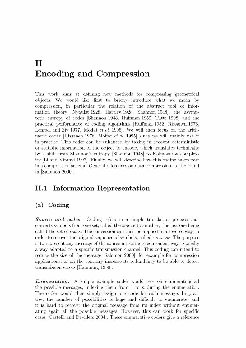
Huffman coder. [Huffman 1952] introduced a simple and efficient coderthat writes each symbol of the source with a code of variable size. Forexample, consider that a digital image is represented by a sequence of colourssblack, sred, sdarkblue, slightblue, swhite. A simple coder will assign a symbol to eachcolour, and encode the image as the sequence of colours. This kind of coderwill be called next an order 0 coder .If the image is a photo of a seascape, as the one of Figure II.1, the probabilityto have blue colours in the message will be higher than for red colours. Huffmanproposed a simple way to encode with less bits the more frequent colours, hereblue ones, and with more bits the less frequent symbols. Consider that eachof the colour probabilities is a power of 2: pblack � 2�3, pred � 2�4, pdarkblue �2�1, plightblue � 2�2, pwhite � 2�4.

21 II.1. Information Representation

Figure II.1: Huffman coding relies on the frequency of symbols of amessage, here the colours inside an image.

These probabilities can be represented by a binary tree, such as each symbolof probability 2�b is a leaf of depth b in the binary tree. Then each symbol isencoded by the left (0) and right (1) choices to get from the root of the tree tothat symbol. The decoding is then performed by following the left and rightcodes until reaching a leaf, and the symbol of that leaf is a new element ofthe decoded message. In that context, the probability of each left and rightoperation is 1

2, which maximises the entropy (h pmq � 1), i.e., the theoretical

performance.

Entropy coder. The original Huffman code also worked out for generalprobabilities, but without maximising the entropy. It uses a greedy algorithm tochoose how to round off the probabilities towards powers of 2 [Huffman 1952].However, Shannon proved that it is asymptotically possible to find a coder ofmaximum entropy [Shannon 1948], and that no other coder can asymptoticallywork better in general. This is the main theoretical justification for thedefinition of h pq. [Huffman 1952] introduced a simpler proof of that theorem,by grouping sequence of symbols until their probability become small enoughto be well approximated by a power of 2.

(c) Levels of Information

In practise, although the entropy of a given coder can be computed, thetheoretical entropy of a source is very hard to seize. The symbols of the sourceare generally not independent, since they represent global information. In thecase of dependent symbols, the entropy would be better computed through theKolmogorov complexity [Li and Vitanyi 1997]. For example, by increasing thecontrast of an image, as human we believe that we loose some of its details,but from the information theory point of view, we added a (mostly) randomvalue to the colours, therefore increasing the information of the image.

An explanation for that phenomenon is that the representation of animage as a sequence of colours is not significant to us. This sequence could beshuffled in a deterministic way, it would not change the coding, but we would

Chapter II. Encoding and Compression 22

not recognise anymore the information of the image. In order to design andevaluate an efficient coding system, we need to represent the exact amountof information that is needed for our application, through an independentset of codes. If we achieve such a coding, then its entropy can be maximisedthrough a universal coder, such as the Huffman coder or the arithmetic coder.

II.2 Arithmetic Coding

The arithmetic coding [Rissanen 1976, Moffat et al. 1995] encodes the symbolssource with code sizes very close to their probabilities. In particular, it achievesan average size of codes that can be a fraction of bits. Moreover, it canencode simultaneously different sources, and provide a flexible way of adaptingprobabilities of the source symbols. This adaptation can be monitored throughrules depending on a context, or automatically looking at the previous encodedsymbols by varying the order of the coder. This section details these points,and provides some sample code inspired from [Arithmetic coding source]. Inparticular, we would like to detail why the arithmetic coder is usually presentedas a universal solution, and how much parameters are hidden behind thisuniversal behaviour. This coder will be used all along this work, and we willdetail for each algorithm the hidden parameters which have a significant impacton the final compression ratio.

(a) Arithmetic Coder

Instead of assigning a code for each of the source symbol, an arithmetic coderrepresent the whole message by a single binary number m P r0, 1r, with a largenumber of digits. Where Huffman decoder read a sequence of left/right codesto rebuild the source message, the arithmetic coder will read a sequence ofinterval shrinking, until finding a small enough interval containing m. At eachstep, the interval is not shrunk by splitting it in two as in Huffman coding, buteach possible symbol of the source is assigned a part of the interval proportionalto its probability, and the interval is shrunk to the part of the source symbol.Therefore, a splitting in two corresponds in general to several shrinking, andthus a single bit can encode many symbols, as the next table details on thebeginning of the example of Figure II.1, using the above probabilities.

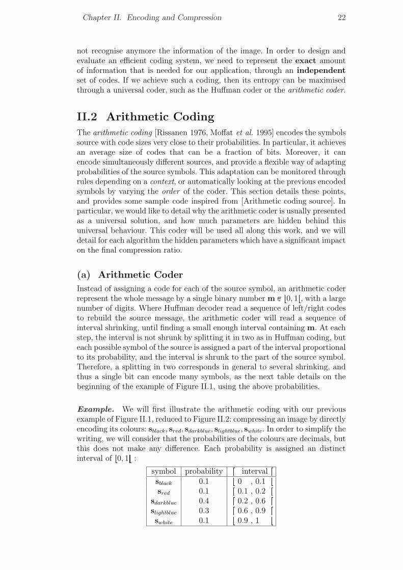
Example. We will first illustrate the arithmetic coding with our previousexample of Figure II.1, reduced to Figure II.2: compressing an image by directlyencoding its colours: sblack, sred, sdarkblue, slightblue, swhite. In order to simplify thewriting, we will consider that the probabilities of the colours are decimals, butthis does not make any difference. Each probability is assigned an distinctinterval of r0, 1r :

symbol probability r interval rsblack 0.1 r 0 , 0.1 rsred 0.1 r 0.1 , 0.2 r

sdarkblue 0.4 r 0.2 , 0.6 rslightblue 0.3 r 0.6 , 0.9 rswhite 0.1 r 0.9 , 1 r

23 II.2. Arithmetic Coding

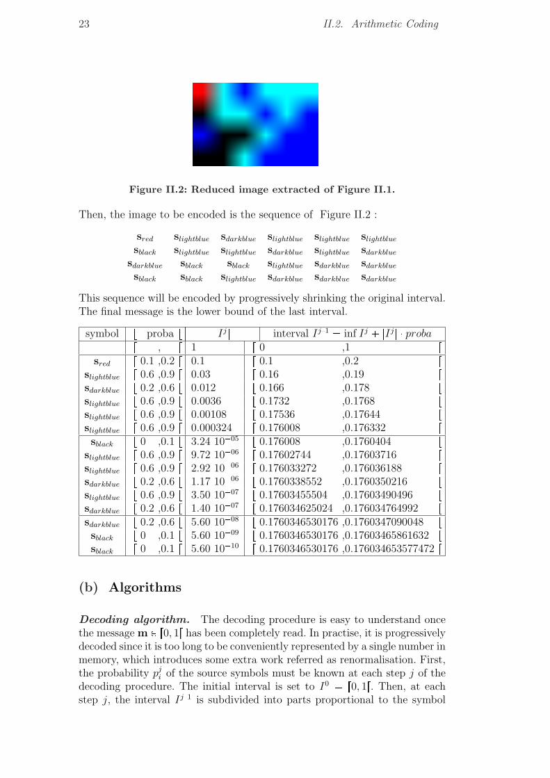
Figure II.2: Reduced image extracted of Figure II.1.

Then, the image to be encoded is the sequence of Figure II.2 :

sred slightblue sdarkblue slightblue slightblue slightblue

sblack slightblue slightblue sdarkblue slightblue sdarkblue

sdarkblue sblack sblack slightblue sdarkblue sdarkblue

sblack sblack slightblue sdarkblue sdarkblue sdarkblue

This sequence will be encoded by progressively shrinking the original interval.The final message is the lower bound of the last interval.

symbol r proba r |Ij| interval Ij�1 � inf Ij � |Ij| � probar , r 1 r 0 ,1 r

sred r 0.1 ,0.2 r 0.1 r 0.1 ,0.2 rslightblue r 0.6 ,0.9 r 0.03 r 0.16 ,0.19 rsdarkblue r 0.2 ,0.6 r 0.012 r 0.166 ,0.178 rslightblue r 0.6 ,0.9 r 0.0036 r 0.1732 ,0.1768 rslightblue r 0.6 ,0.9 r 0.00108 r 0.17536 ,0.17644 rslightblue r 0.6 ,0.9 r 0.000324 r 0.176008 ,0.176332 rsblack r 0 ,0.1 r 3.24 10�05 r 0.176008 ,0.1760404 r

slightblue r 0.6 ,0.9 r 9.72 10�06 r 0.17602744 ,0.17603716 rslightblue r 0.6 ,0.9 r 2.92 10�06 r 0.176033272 ,0.176036188 rsdarkblue r 0.2 ,0.6 r 1.17 10�06 r 0.1760338552 ,0.1760350216 rslightblue r 0.6 ,0.9 r 3.50 10�07 r 0.17603455504 ,0.17603490496 rsdarkblue r 0.2 ,0.6 r 1.40 10�07 r 0.176034625024 ,0.176034764992 rsdarkblue r 0.2 ,0.6 r 5.60 10�08 r 0.1760346530176 ,0.1760347090048 rsblack r 0 ,0.1 r 5.60 10�09 r 0.1760346530176 ,0.17603465861632 rsblack r 0 ,0.1 r 5.60 10�10 r 0.1760346530176 ,0.176034653577472 r

(b) Algorithms

Decoding algorithm. The decoding procedure is easy to understand oncethe message m P r0, 1r has been completely read. In practise, it is progressivelydecoded since it is too long to be conveniently represented by a single number inmemory, which introduces some extra work referred as renormalisation. First,the probability pj

i of the source symbols must be known at each step j of thedecoding procedure. The initial interval is set to I0 � r0, 1r. Then, at eachstep j, the interval Ij�1 is subdivided into parts proportional to the symbol

Chapter II. Encoding and Compression 24

probabilities pji into subintervals sIj

i as follows :

sIj1 � [ 0 , pj

1 [

sIj2 � [ pj

1 , pj1 � pj

2 [

sIj3 � [ pj

1 � pj2 , pj

1 � pj2 � pj

3 [� � �sIj

n�1 � [ 1� pjn � pj

n�1 , 1� pjn [

sIjn � [ 1� pj

n , 1 [

Then, the message m belongs to one of the subintervals sIji , corresponding

to symbol si. This symbol si is added to the decoded message, and the nextinterval is set to sIj

i : Ij � sIji .

Algorithm 1 aritdecode(in,out) : decodes stream in to out

1: I Ð r0, 1r // initial interval

2: in�32ÝÝÑm // reads the first bits of the input

3: repeat4:5: ppiqiPv1,nw Ð get model pq // retrieves the probabilities

6: count Ð p1 // upper bound of sIji

7: for i P v2, nw do // look the interval containing m8: if m   count then // found the subinterval9: break // exits the for loop

10: end if11: count Ð count� pi // next i12: end for13:14: sÐ si ; out

�sÐÝ si // decoded symbol si

15: I Ð rcount� pi�1, countr // updates the current interval16:17: while 1

2R I or |I|   1

2do // renormalisation

18: if I � �12, 1�then // higher half

19: I Ð I � 12

; mÐm� 12

// shifts higher half to lower half20: else if I � �

14, 3

4

�then // central half

21: I Ð I � 14

; mÐm� 14

// shifts central half to lower half22: end if23: I Ð 2 � I // lower half is directly renormalised

24: mÐ 2 �m ; in�1ÝÑm // message is shifted by reading in

25: end while26:27: until s � stop // read a stop symbol

Renormalisation. Observe that unless the decoder does not stop on itsown, as for Huffman coding. The source must have a stop symbol or thedecompression must know how to stop the decoder. For large messages, theintervals Ij require more memory to be represented than the usual 2� 64 bits

25 II.2. Arithmetic Coding

offered by computers. Therefore, when an interval Ij is contained in�0, 1

2

�or�

12, 1�, one bit of the message is transmitted, the interval is shifted (scaled by

two), and the algorithm goes on. Moreover, the intervals Ij can get arbitrarilysmall around 1

2. In order to prevent this, when Ij � �

14, 3

4

�, two bits of the

message are transmitted, the interval is shifted twice (scaled by four). Theseprocesses are called renormalisation. In parallel, the message does not need tobe read entirely, since the only precision needed to decode one symbol is givenby the intervals Ij. At each renormalisation, a complement of the message isread to ensure that the precision of the interval matches the precision of themessage. This whole process is implemented by Algorithm 1: aritdecode.

Algorithm 2 aritencode(in,out) : encodes stream in to out

1: I Ð r0, 1r // initial interval2: repeat3: ppiqiPv1,nw Ð get model pq // retrieves the probabilities

4: in�sÝÑ si // retrieves symbol to encode

5: I Ð �°kPv1,i�1w pk,

°kPv1,iw pk

�// deduce the current interval

6: while 12R I or |I|   1

2do // renormalisation

7: if I � �0, 1

2

�then // lower half

8: out�1ÐÝ 0 // appends a 0 to the coded message

9: else if I � �12, 1�then // higher half

10: out�1ÐÝ 1 // appends a 1 to the coded message

11: I Ð I � 12

// shifts higher half to lower half12: else if I � �

14, 3

4

�then // central half

13: out.repeat next bit // set out to repeat the next bit to be output14: I Ð I � 1

4// shifts central half to lower half

15: end if16: I Ð 2 � I // scaling17: end while18:19: until s � stop // read a stop symbol

Encoding algorithm. The encoding procedure is very similar to the decod-ing one, as details on Algorithm 2: aritencode. Note that in both cases, the finiteprecision of computer representations forces to use only half of the availablebits to represent the probabilities and the intervals, since both have to be mul-tiplied with exact precision. Also, the open intervals are actually representedby closed ones: rni, nsr � rni, ns�1r.

(c) Statistical Modelling

This arithmetic coder provides a powerful engine to encode a universal source.However, it is very sensible to the tuning, which is a very hard task. First, theprobability model is very important. Consider a zero–entropy message, i.e. amessage with a constant symbol s0. If the probability model states that s0 hasprobability p0 ! 1, then the encoded stream will have a huge length. Therefore,

Chapter II. Encoding and Compression 26

the arithmetic coder is not close to an entropy coder, unless very well tuned.We will see some generic techniques to improve these aspects.

Adaptive models. A simple solution to the adaptability of the probabilitiesconsists in updating the probability model along the encoding, in a determin-istic way. For example, the probability of a symbol can increase each time it isencoded, or the probability of a stop symbol can increase at each new symbolencoded, as on the table below. This can be easily implemented through thefunction get modelpq of Algorithm 1: aritdecode and Algorithm 2: aritencode. Forthe case of the zero–entropy stream, there would be a reasonable amount ofencoded stream where p0 goes closer to 1, and then the stream will be encodedat a better rate. Observe that p0 cannot reach one, since the probability of eachsymbol must not vanish, prohibiting an asymptotic zero–length, but respectingthe second item of the requirements for the entropy of Section II.1(b) Informa-tion Theory.

symbol updated probabilites r ps r |Ij| Ij�1010

110

210

610

910

1010

r , r 1 r 0 ,1 rsred

011

111

311

711

1011

1111

r 110

, 210r 0.1 r 0.1 ,0.2 r

slightblue012

112

312

712

1112

1212

r 711

,1011r 0.027272 r 0.16363636 ,0.19090909 r

sdarkblue013

113

313

813

1213

1313

r 312

, 712r 0.009090 r 0.17045454 ,0.17954546 r

slightblue014

114

314

814

1314

1414

r 813

,1213r 0.002797 r 0.17604895 ,0.17884615 r

slightblue015

115

315

815

1415

1515

r 814

,1314r 0.000999 r 0.17764735 ,0.17864635 r

slightblue016

116

316

816

1516

1616

r 815

,1415r 0.000400 r 0.17818015 ,0.17857975 r

sblack017

217

417

917

1617

1717

r 016

, 116r 2.49 10�5 r 0.17818015 ,0.17820513 r

slightblue018

218

418

918

1718

1818

r 917

,1617r 1.02 10�5 r 0.17819337 ,0.17820366 r

slightblue019

219

419

919

1819

1919

r 918

,1718r 4.57 10�6 r 0.17819851 ,0.17820309 r

sdarkblue020

220

420

1020

1920

2020

r 419

, 919r 1.20 10�6 r 0.17819948 ,0.17820068 r

slightblue021

221

421

1021

2021

2121

r 1020

,1920r 5.41 10�7 r 0.17820008 ,0.17820062 r

sdarkblue022

222

422

1122

2122

2222

r 421

,1021r 1.54 10�7 r 0.17820018 ,0.17820034 r

sdarkblue023

223

423

1223

2223

2323

r 422

,1122r 4.92 10�8 r 0.17820021 ,0.17820026 r

sblack024

324

524

1324

2324

2424

r 023

, 223r 4.27 10�9 r 0.17820021 ,0.17820022 r

sblack025

425

625

1425

2425

2525

r 024

, 324r 0.53 10�9 r 0.17820021 ,0.17820021 r

Order. This probability model can be enhanced by considering groups ofsymbols instead of only one. The number of symbols considered jointly iscalled the order of the coder. This is particularly useful for text, where syllablesplay an important role. An order 0 coder means that the probability model isupdated continuously, whereas an order k model will use a different probabilitymodel for each combination of the k symbols preceding the encoded one.

Contexts. With this point of view, the arithmetic coder begins with oneprobability model, and updates it continuously along the encoding process.However, we can actually consider various probability models simultaneously,

27 II.3. Compression

depending on the context of the symbol to encode. For example when codinga text, it is more probable to find a vowel after a consonant. Therefore, theprobability of a vowel after another vowel could be reduced to improve theprobability model.

Limits. Context modelling and order–based coding allows reducing theinterdependence of the symbols (putting the entropy closer to the Kolmogorovcomplexity [Li and Vitanyi 1997]). This process is the main part of describingthe object to encode, but since it is a difficult one, these features can lead tosignificant improvements of the results. However, the number of contexts andthe order must be limited, since for each context the coder builds a probabilitymodel through the regular updates, and an exponential number for each orderadded. This probability needs a reasonable amount of encoded stream to getcloser to the real probability model. The encoded stream must be longer thanthis amount of time for each context.

Prediction. Another way to reduce the covariance relies on predictionmechanisms, i.e. deductions that can be equally obtained from the encoderand the decoder. Since we encode the lower part of the interval containingthe message, a message ended by a sequence of 0 is cheaper to encode than amessage ended with a 1, as on the example of Section II.2(a) Arithmetic Coder .Therefore, if the prediction always asserts the results, the message will be asequence of 0s, with some isolated 1s. This is actually encoded by an arithmeticcoder as a run–length encoded stream, since the stop characters induce a verytiny last interval. If the stop can be predicted too, then the arithmetic codingspares the last sequence of 0s. In this rough point of view, the better case ofarithmetic coding is, for a generic problem, the logarithm of the number ofsymbols.

II.3 CompressionCoding is only a part of a compression scheme. Actually, a compression schemeis composed of various steps of conversions, from the original data to a symbolicrepresentation, from this representation to specifications of sources, from thesesources to the encoded message, from this encoded message to a transmissionprotocol, which entails a re–coding for error detection, and the symmetric partsfrom the receiver.

This whole process can be designed part by part, or all together. Forexample, some nice compression scheme already contains error detection usingthe redundancy of the original data that is left after the encoding. Some lossyor progressive compression schemes perform the encoding directly from therepresentation and incorporate the specification of sources.

These features optimise compression for specific applications. However,a generic application usually requires a separate design of the parts of acompression scheme. In this context, arithmetic coding turns out to be avery flexible tool to work on the final compression ratio, i.e. the ratio of thefinal size and the original size of the data. Depending on the application, this

Chapter II. Encoding and Compression 28

compression ratio must be reduced to optimize specific characteristics of theseapplications, leading to different trade–offs. We will now detail three suchgeneric trade–offs.

(a) Compaction

Compaction refers to compact data structures, also called succinct. Thesestructures aim at reducing the size of the memory used during the execution ofan application, while maintaining a small execution overhead. This trade–offbetween memory used and execution time must also allow a random access tothe compact data structure. For example for mesh data structures, this trade–off can be simply a elegant data representation with no specific encoding suchas [Rossignac et al. 2001, Lage et al. 2005*1, Lage et al. 2005]. It can also in-volve simple encoding scheme that are fast to interpret as [Houston et al. 2005],or involve a precise mixture of very efficient encoding with a higher–level datastructure, such as [Castelli et al. 2005*1, Castelli et al. 2005*2].

(b) Direct Compression

The most used meaning of compression refers to file compression or tocompression of exchanged information. Most of the common generic algo-rithms are based on the LZH (ZIP) algorithm of [Lempel and Ziv 1977],aside from specific image and video compression algorithms such asJPEG [Wallace 1991, Christopoulos et al. 2000] and MPEG [le Gall 1991,Pereira and Ebrahimi 2002]. In this case, the goal is to optimise the trade–off between compression rate and compression time: the enumeration methodis usually too slow, while a simple coding of the data representation can be ingeneral improved with a minor time overhead. The trade–off can also takeinto account the amount of memory necessary to compress or decompressthe stream. In that case, the process is usually performed out–of–core, suchas [Isenburg and Gumhold 2003].

(c) Progressive Compression

The compression can also lead to a loss of information when decompressing.This can be useful either when the lost part is not significant, or when itcan be recovered by a further step of the compression. In that second sense,lossy compression will generate objects at various levels of detail, i.e. in multi-resolution. Each resolution can be compressed separately by the differencefrom the previous one. A variant of that scheme does not distinguish betweenlevels of details, sending a coarse level by direct compression, and refining itby a sequence of local changes. In these contexts, the goal is to optimise thetrade–off between compression ratio and the distortion of the decompressedmodel. For the geometrical models, the distortion is usually measured by thegeometric distance between the decoded model and the original one.

IIIMeshes and Geometry

Geometrical objects are usually represented through meshes. Especially forsurfaces in the space, triangulations had the advantage for rendering ofrepresenting with a single element (a triangle) many pixels on screen, whichreduced the number of elements to store. Although the increasing size of usualmeshes reduced this advantage, graphic hardware and algorithms are optimisedfor these representations and meshes are still predominant over point setsmodels. Moreover, several parts of the alternative to meshes require local meshgeneration, which becomes very costly in higher dimensions. Finally, meshesdescribe in a unique and explicit manner the support of the geometrical object,either by piecewise interpolation or by local parameterisation such as splinesor NURBS.

To a real object correspond several meshes. These meshes represent thesame geometry and topology, and thus differ by their connectivity . The waythese objects are discretised usually depends on the application, varying fromvisualisation to animation and finite element methods. These variations makeit harder to define the geometric quality of a mesh independently of theapplication, even with a common definition for the connectivity.

This chapter details the combinatorial part, introducing the definitionand properties of meshes in Section III.1 Simplicial Complexes and Polytopes, anda complete set of operations on the connectivity in Section III.2 CombinatorialOperators. Finally, Section III.3 Geometry and Discretisation gives some classicalexamples of interactions of geometry and meshes.

In this work, we do not use a specific data structure for meshes. We willconsider the operations described in this chapter as the basic elements of ageneric data structure. For further readings, the classical data structures forsurfaces are the winged–edge [Baumgart 1972], the split–edge [Eastman 1982],the quad–edge [Guibas and Stolfi 1985], the half–edge [Mantyla 1988]and the corner–table [Rossignac et al. 2001, Lage et al. 2005]. For non–manifold 2–meshes, we would mention the radial–edge [Weiler 1985]and [de Floriani and Hui 2003]. Further references on the following definitionscan be found in [Munkres 1984, Boissonnat and Yvinec 1998, Hatcher 2002].

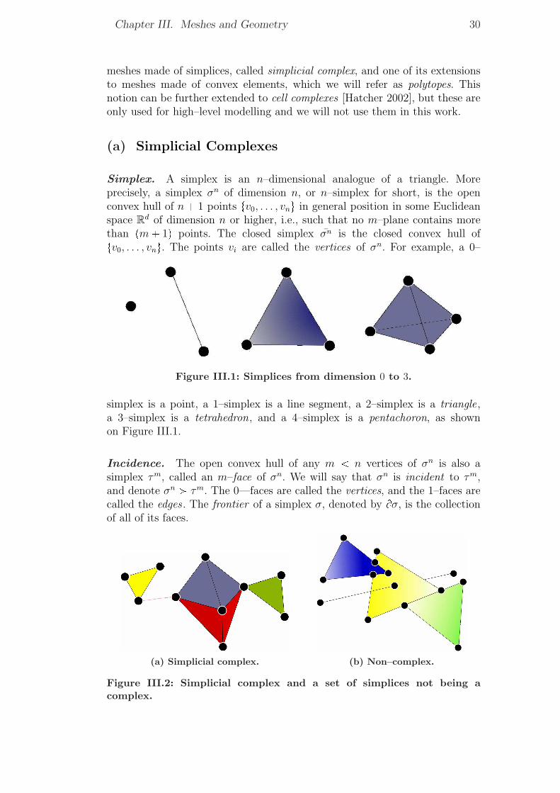
III.1 Simplicial Complexes and PolytopesThere are various kind of meshes used in Computer Graphics, ScientificVisualisation, Geometric Modelling and Geometry Processing. However, thegraphic hardware is optimised for processing triangles, line segments andpoints, which are all special cases of simplices. We will therefore focus mainly on

Chapter III. Meshes and Geometry 30

meshes made of simplices, called simplicial complex, and one of its extensionsto meshes made of convex elements, which we will refer as polytopes. Thisnotion can be further extended to cell complexes [Hatcher 2002], but these areonly used for high–level modelling and we will not use them in this work.

(a) Simplicial Complexes

Simplex. A simplex is an n–dimensional analogue of a triangle. Moreprecisely, a simplex σn of dimension n, or n–simplex for short, is the openconvex hull of n � 1 points tv0, . . . , vnu in general position in some Euclideanspace Rd of dimension n or higher, i.e., such that no m–plane contains morethan pm� 1q points. The closed simplex σn is the closed convex hull oftv0, . . . , vnu. The points vi are called the vertices of σn. For example, a 0–

Figure III.1: Simplices from dimension 0 to 3.

simplex is a point, a 1–simplex is a line segment, a 2–simplex is a triangle,a 3–simplex is a tetrahedron, and a 4–simplex is a pentachoron, as shownon Figure III.1.

Incidence. The open convex hull of any m   n vertices of σn is also asimplex τm, called an m–face of σn. We will say that σn is incident to τm,and denote σn ¡ τm. The 0—faces are called the vertices, and the 1–faces arecalled the edges . The frontier of a simplex σ, denoted by Bσ, is the collectionof all of its faces.

(a) Simplicial complex. (b) Non–complex.

Figure III.2: Simplicial complex and a set of simplices not being acomplex.

31 III.1. Simplicial Complexes and Polytopes

Complex. A simplicial complex K of Rd is a coherent collection of simplicesof Rd, where coherent means that K contains all the faces of each simplex(@σ P K, Bσ � K), and contains also the geometrical intersection of theclosure of any two simplices (@ pσ1, σ2q P K2, σ1 X σ2 � K), as illustratedon Figure III.2. Two simplices incident to a common simplex are said to beadjacent . The geometry of a complex usually refers to the coordinates of itsvertices, while its connectivity refers to the incidence of higher–dimensionalsimplices on these vertices.

Skeleton. If a collection K 1 of simplices of K is a simplicial complex, thenit is called a subcomplex of K. The subcomplex Kpmq of all the p–simplices,p ¤ m, is called the m–skeleton of K.

Connected components. A complex is connected if it cannot be repre-sented as a union of two non–empty disjoint subcomplexes. A component of acomplex K is a maximal connected subcomplex of K.

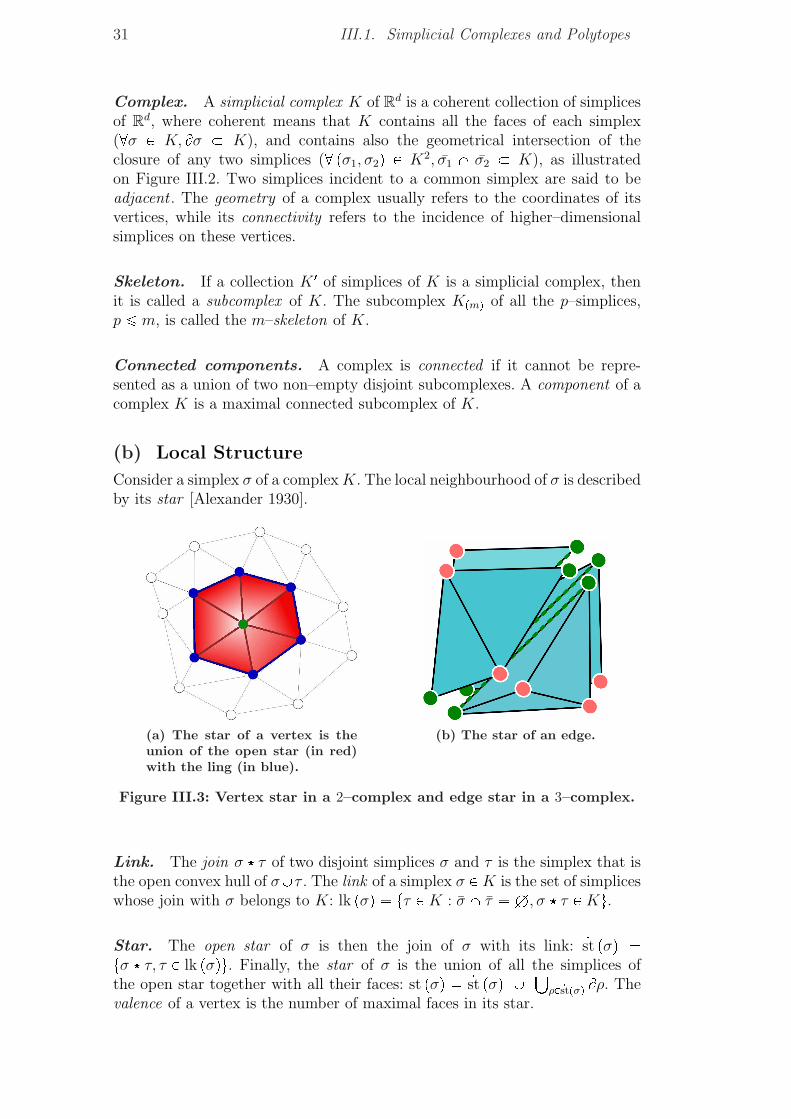
(b) Local Structure

Consider a simplex σ of a complex K. The local neighbourhood of σ is describedby its star [Alexander 1930].

(a) The star of a vertex is theunion of the open star (in red)with the ling (in blue).

(b) The star of an edge.

Figure III.3: Vertex star in a 2–complex and edge star in a 3–complex.

Link. The join σ � τ of two disjoint simplices σ and τ is the simplex that isthe open convex hull of σYτ . The link of a simplex σ P K is the set of simpliceswhose join with σ belongs to K: lk pσq � tτ P K : σ X τ � H, σ � τ P Ku.Star. The open star of σ is then the join of σ with its link: 9st pσq �tσ � τ, τ P lk pσqu. Finally, the star of σ is the union of all the simplices ofthe open star together with all their faces: st pσq � 9st pσq Y �

ρP 9stpσq Bρ. Thevalence of a vertex is the number of maximal faces in its star.

Chapter III. Meshes and Geometry 32

(c) Pure Simplicial Complexes

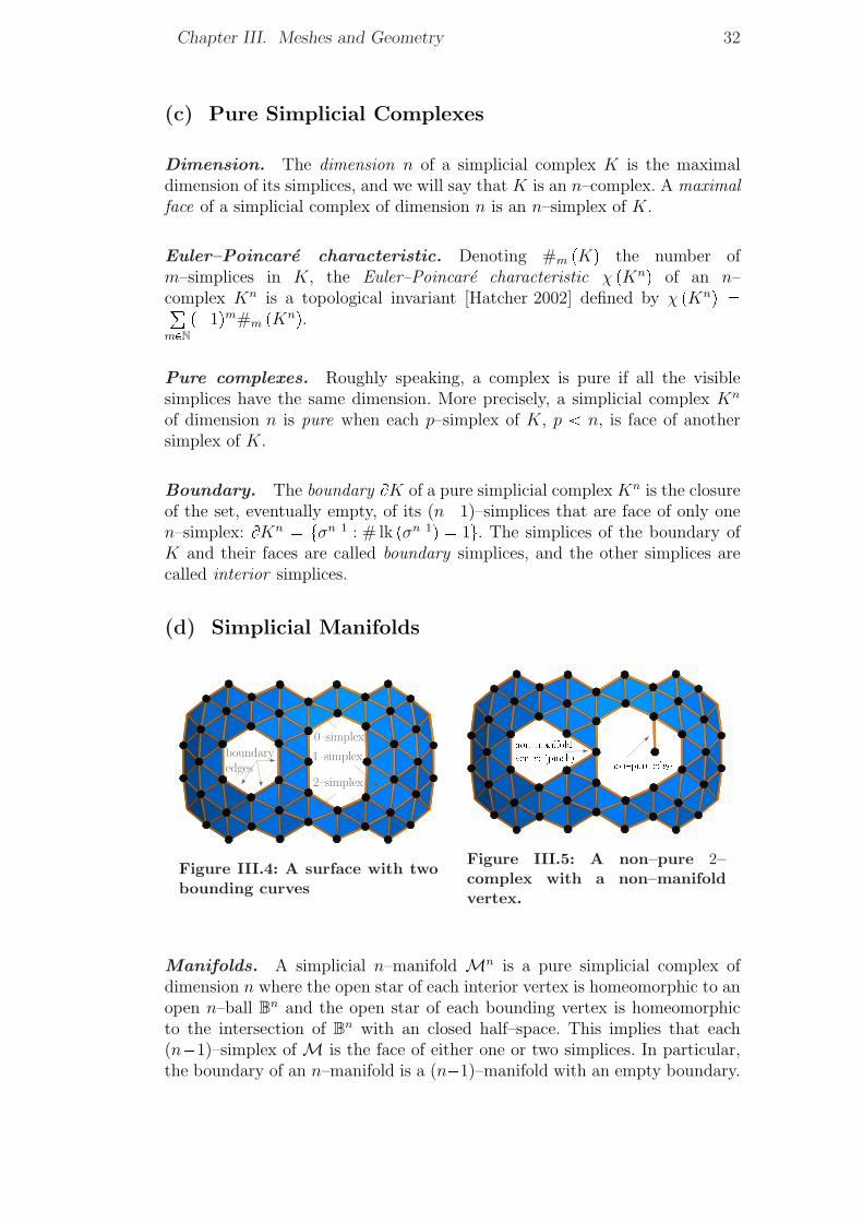
Dimension. The dimension n of a simplicial complex K is the maximaldimension of its simplices, and we will say that K is an n–complex. A maximalface of a simplicial complex of dimension n is an n–simplex of K.

Euler–Poincare characteristic. Denoting #m pKq the number ofm–simplices in K, the Euler–Poincare characteristic χ pKnq of an n–complex Kn is a topological invariant [Hatcher 2002] defined by χ pKnq �°mPNp�1qm#m pKnq.

Pure complexes. Roughly speaking, a complex is pure if all the visiblesimplices have the same dimension. More precisely, a simplicial complex Kn

of dimension n is pure when each p–simplex of K, p   n, is face of anothersimplex of K.

Boundary. The boundary BK of a pure simplicial complex Kn is the closureof the set, eventually empty, of its (n�1)–simplices that are face of only onen–simplex: BKn � tσn�1 : # lk pσn�1q � 1u. The simplices of the boundary ofK and their faces are called boundary simplices, and the other simplices arecalled interior simplices.

(d) Simplicial Manifolds

Figure III.4: A surface with twobounding curves

Figure III.5: A non–pure 2–complex with a non–manifoldvertex.

Manifolds. A simplicial n–manifold Mn is a pure simplicial complex ofdimension n where the open star of each interior vertex is homeomorphic to anopen n–ball Bn and the open star of each bounding vertex is homeomorphicto the intersection of Bn with an closed half–space. This implies that each(n�1)–simplex of M is the face of either one or two simplices. In particular,the boundary of an n–manifold is a (n�1)–manifold with an empty boundary.

33 III.1. Simplicial Complexes and Polytopes

Orientability. An orientation on a simplex is an ordering pv0, . . . , vnq on itsvertices. Two orientations are equivalent if they differ by an even permutation.There are therefore two opposite orientations on a simplex. A simplicialmanifold Mn is orientable when it is possible to choose a coherent orientationon all its simplices. More precisely, if σn�1 � pv1, . . . , vnq is an oriented interior(n�1)–simplex ofMn, face of ρ � σn�1�v and ρ1 � σn�1�v1, then the orientationof ρ and ρ1 is coherent the orientation of ρ is equivalent to pv, v1, . . . , vnq andthe orientation of ρ1 is opposed to pv1, v1, . . . , vnq. This orientation thus definesthe notion of next and previous vertex inside a triangle of a simplex.

Surfaces. For example, a 2–manifold is a surface, i.e. a simplicial complexmade of only vertices, edges and triangles where each edge is in the frontierof either one or two triangles and where the boundary does not pinch.For example, Figure III.4 shows an example of 2–manifold and Figure III.5illustrates a 2–complex that is neither pure nor a manifold. The topology ofsurfaces can be easily defined from its orientability and its Euler–Poincarecharacteristic, using the Surface classification theorem [Armstrong 1979]: Anyoriented connected surface S is homeomorphic to either the sphere S2 (g pSq �0) or a connected sum of g pSq ¡ 0 tori, in both cases with some finite numberb pSq of open disks removed. The number g pSq is called the genus of S, andb pSq its number of boundaries. The Euler–Poincare characteristic χ pSq of Sis equal to χ pSq � #2 pSq �#1 pSq �#0 pSq � 2� 2 � g pSq � b pSq.

(e) Polytopes

Surfaces in finite element methods are usually represented by a mixture oftriangular and quadrangular elements. Although this do not directly fits to thesimplicial complexes we just introduced, this structure can be easily extendedto that case. For example, one could divide each quadrangle into two coplanartriangles and get a simplicial complex. We define a polytope in a similar way.

Along this work, a polytope in Rd will be a coherent collection of convexopen set of Rd, called cells , where coherent means again that the collectioncontains the frontiers and the intersections of its cells. Observe that this impliesthat each cell is made up with piecewise linear elements, from edges to itsmaximal faces.

The definition and properties described above are still valid, in particularthe notion of boundary, manifold, orientability, and the classification for 2–dimensional manifold polytopes. Moreover, polytopes are useful to define thedual of a manifold: The dual of an n–manifold Md is the manifold polytopeobtained by reversing the incidence relations of its cells, i.e. creating a vertexfor each n–cell of Md, and an m–cell for each (n�m)–cell of Md, spanningthe vertices created for each n–cell of its star in Md.

Chapter III. Meshes and Geometry 34

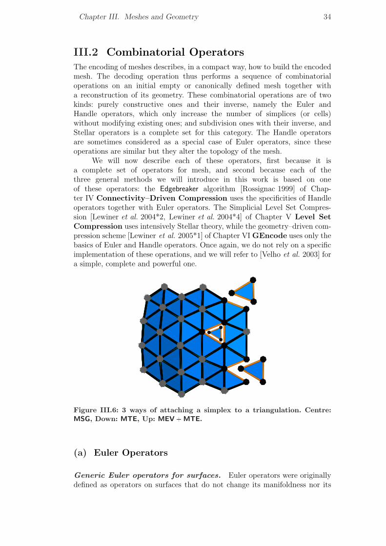
III.2 Combinatorial OperatorsThe encoding of meshes describes, in a compact way, how to build the encodedmesh. The decoding operation thus performs a sequence of combinatorialoperations on an initial empty or canonically defined mesh together witha reconstruction of its geometry. These combinatorial operations are of twokinds: purely constructive ones and their inverse, namely the Euler andHandle operators, which only increase the number of simplices (or cells)without modifying existing ones; and subdivision ones with their inverse, andStellar operators is a complete set for this category. The Handle operatorsare sometimes considered as a special case of Euler operators, since theseoperations are similar but they alter the topology of the mesh.

We will now describe each of these operators, first because it isa complete set of operators for mesh, and second because each of thethree general methods we will introduce in this work is based on oneof these operators: the Edgebreaker algorithm [Rossignac 1999] of Chap-ter IV Connectivity–Driven Compression uses the specificities of Handleoperators together with Euler operators. The Simplicial Level Set Compres-sion [Lewiner et al. 2004*2, Lewiner et al. 2004*4] of Chapter V Level SetCompression uses intensively Stellar theory, while the geometry–driven com-pression scheme [Lewiner et al. 2005*1] of Chapter VI GEncode uses only thebasics of Euler and Handle operators. Once again, we do not rely on a specificimplementation of these operations, and we will refer to [Velho et al. 2003] fora simple, complete and powerful one.

Figure III.6: 3 ways of attaching a simplex to a triangulation. Centre:MSG, Down: MTE, Up: MEV �MTE.

(a) Euler Operators

Generic Euler operators for surfaces. Euler operators were originallydefined as operators on surfaces that do not change its manifoldness nor its

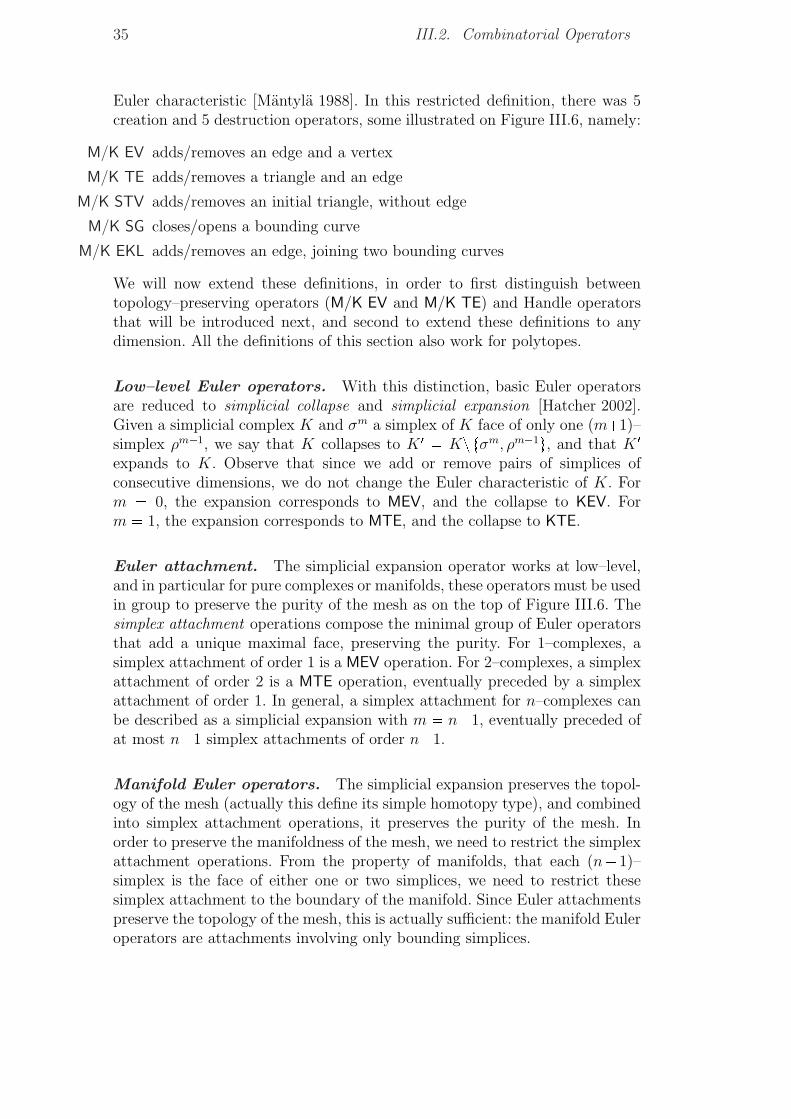
35 III.2. Combinatorial Operators

Euler characteristic [Mantyla 1988]. In this restricted definition, there was 5creation and 5 destruction operators, some illustrated on Figure III.6, namely:

M/K EV adds/removes an edge and a vertex

M/K TE adds/removes a triangle and an edge

M/K STV adds/removes an initial triangle, without edge

M/K SG closes/opens a bounding curve

M/K EKL adds/removes an edge, joining two bounding curves

We will now extend these definitions, in order to first distinguish betweentopology–preserving operators (M/K EV and M/K TE) and Handle operatorsthat will be introduced next, and second to extend these definitions to anydimension. All the definitions of this section also work for polytopes.

Low–level Euler operators. With this distinction, basic Euler operatorsare reduced to simplicial collapse and simplicial expansion [Hatcher 2002].Given a simplicial complex K and σm a simplex of K face of only one (m�1)–simplex ρm�1, we say that K collapses to K 1 � Kz tσm, ρm�1u, and that K 1expands to K. Observe that since we add or remove pairs of simplices ofconsecutive dimensions, we do not change the Euler characteristic of K. Form � 0, the expansion corresponds to MEV, and the collapse to KEV. Form � 1, the expansion corresponds to MTE, and the collapse to KTE.

Euler attachment. The simplicial expansion operator works at low–level,and in particular for pure complexes or manifolds, these operators must be usedin group to preserve the purity of the mesh as on the top of Figure III.6. Thesimplex attachment operations compose the minimal group of Euler operatorsthat add a unique maximal face, preserving the purity. For 1–complexes, asimplex attachment of order 1 is a MEV operation. For 2–complexes, a simplexattachment of order 2 is a MTE operation, eventually preceded by a simplexattachment of order 1. In general, a simplex attachment for n–complexes canbe described as a simplicial expansion with m � n�1, eventually preceded ofat most n�1 simplex attachments of order n�1.

Manifold Euler operators. The simplicial expansion preserves the topol-ogy of the mesh (actually this define its simple homotopy type), and combinedinto simplex attachment operations, it preserves the purity of the mesh. Inorder to preserve the manifoldness of the mesh, we need to restrict the simplexattachment operations. From the property of manifolds, that each (n�1)–simplex is the face of either one or two simplices, we need to restrict thesesimplex attachment to the boundary of the manifold. Since Euler attachmentspreserve the topology of the mesh, this is actually sufficient: the manifold Euleroperators are attachments involving only bounding simplices.

Chapter III. Meshes and Geometry 36

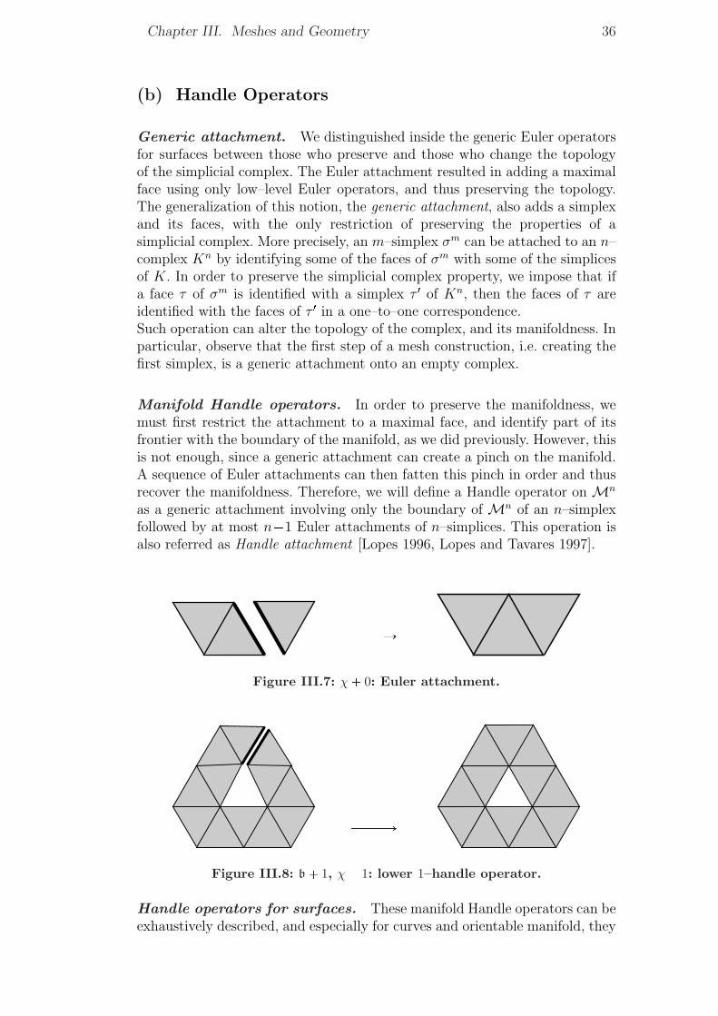
(b) Handle Operators

Generic attachment. We distinguished inside the generic Euler operatorsfor surfaces between those who preserve and those who change the topologyof the simplicial complex. The Euler attachment resulted in adding a maximalface using only low–level Euler operators, and thus preserving the topology.The generalization of this notion, the generic attachment, also adds a simplexand its faces, with the only restriction of preserving the properties of asimplicial complex. More precisely, an m–simplex σm can be attached to an n–complex Kn by identifying some of the faces of σm with some of the simplicesof K. In order to preserve the simplicial complex property, we impose that ifa face τ of σm is identified with a simplex τ 1 of Kn, then the faces of τ areidentified with the faces of τ 1 in a one–to–one correspondence.Such operation can alter the topology of the complex, and its manifoldness. Inparticular, observe that the first step of a mesh construction, i.e. creating thefirst simplex, is a generic attachment onto an empty complex.

Manifold Handle operators. In order to preserve the manifoldness, wemust first restrict the attachment to a maximal face, and identify part of itsfrontier with the boundary of the manifold, as we did previously. However, thisis not enough, since a generic attachment can create a pinch on the manifold.A sequence of Euler attachments can then fatten this pinch in order and thusrecover the manifoldness. Therefore, we will define a Handle operator on Mn

as a generic attachment involving only the boundary of Mn of an n–simplexfollowed by at most n�1 Euler attachments of n–simplices. This operation isalso referred as Handle attachment [Lopes 1996, Lopes and Tavares 1997].

ÝÝÝÝÝÑ

Figure III.7: χ� 0: Euler attachment.

ÝÝÝÝÝÑ

Figure III.8: b� 1, χ� 1: lower 1–handle operator.

Handle operators for surfaces. These manifold Handle operators can beexhaustively described, and especially for curves and orientable manifold, they

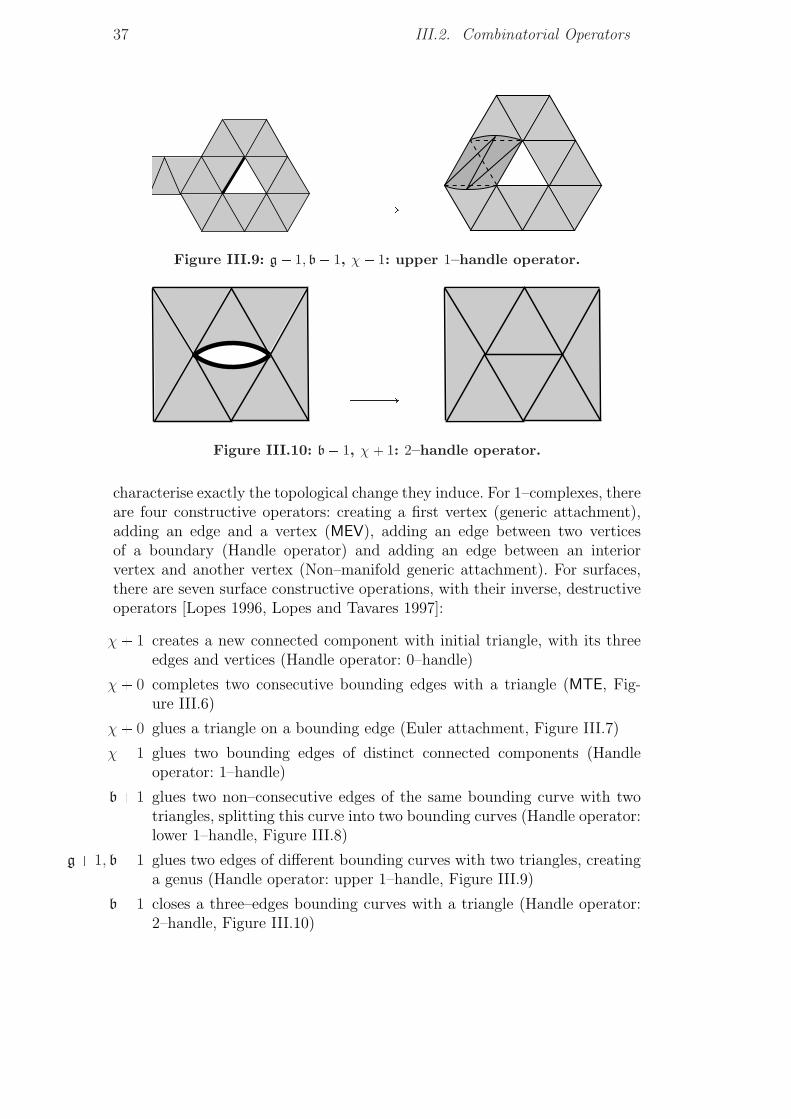
37 III.2. Combinatorial Operators

ÝÝÝÝÝÑ

Figure III.9: g� 1, b� 1, χ� 1: upper 1–handle operator.

ÝÝÝÝÝÑ

Figure III.10: b� 1, χ� 1: 2–handle operator.

characterise exactly the topological change they induce. For 1–complexes, thereare four constructive operators: creating a first vertex (generic attachment),adding an edge and a vertex (MEV), adding an edge between two verticesof a boundary (Handle operator) and adding an edge between an interiorvertex and another vertex (Non–manifold generic attachment). For surfaces,there are seven surface constructive operations, with their inverse, destructiveoperators [Lopes 1996, Lopes and Tavares 1997]:

χ� 1 creates a new connected component with initial triangle, with its threeedges and vertices (Handle operator: 0–handle)

χ� 0 completes two consecutive bounding edges with a triangle (MTE, Fig-ure III.6)

χ� 0 glues a triangle on a bounding edge (Euler attachment, Figure III.7)

χ� 1 glues two bounding edges of distinct connected components (Handleoperator: 1–handle)

b� 1 glues two non–consecutive edges of the same bounding curve with twotriangles, splitting this curve into two bounding curves (Handle operator:lower 1–handle, Figure III.8)

g� 1, b� 1 glues two edges of different bounding curves with two triangles, creatinga genus (Handle operator: upper 1–handle, Figure III.9)

b� 1 closes a three–edges bounding curves with a triangle (Handle operator:2–handle, Figure III.10)

Chapter III. Meshes and Geometry 38

(c) Stellar Operators

Stellar theory. Stellar theory studies the combinatorial equivalencesbetween simplicial complexes. It was developed by [Newman 1926]and [Alexander 1930], and more recently consolidated by [Pachner 1991]and [Lickorish 1999]. This theory states another class of operators for editingthe combinatorial structure of a manifold with a minimal set of operatorswhile preserving its topology. As opposed to Euler and Handle operators,stellar operators intend to modify, as opposed to constructing meshes. Thestellar operators were first stated in [Alexander 1930] as stellar moves, andthen reformulated in [Pachner 1991] as bistellar moves. Both cases can bedecomposed on edges with the vertex weld and edge split operations.

Stellar moves. A stellar move of order m on a simplicial complex K consistsof replacing the star of an m–simplex σm by the join of a vertex with the linkof σm: K Ñ Kz st pσq Y v � lk pσq. These moves are a powerful operation, asstated in Alexander’s theorem [Newman 1926, Glaser 1970, Theorem II.17]:Any two simplicial complexes are piecewise–linear homeomorphic if and onlyif they are related by a finite sequence of stellar moves.

Bistellar moves. Bistellar moves are somehow more concise than stellarmoves, and can be defined as follows. Consider an m–simplex σm of ansimplicial complex Kn of dimension n, and an pn � mq–simplex τn�m notincluded in Kn, such that lk pσmq � Bτn�m. Then the complex Kn z σm �Bτn�m Y Bσm � τn�m is said to be obtained from Kn by a bistellar moveof order m. Note that the inverse of a bistellar move of order m is a bi-stellar move of order (n �m), and that, for manifolds, a bistellar move doesnot change the connectivity of the boundary. [Pachner 1991] proved a similartheorem as Alexander’s one: two simplicial manifolds with an empty boundaryare equivalent if and only if they are related by a finite sequence of bistellarmoves.

Weld and split. Actually, Stellar theory states that stellar moveson edges are sufficient to map any two equivalent combinatorial mani-folds [Alexander 1930]. This can be proved by decomposing the bistellar movesby stellar moves on edges. The stellar move on edge is called an edge split, andthe inverse operation, which removes the inserted vertex, is called a vertex weld.Therefore, stellar operations can be used as primitives for multiresolution op-erators. In particular, an edge flip [Hoppe et al. 1993] can be decomposed as anedge split followed by a vertex weld. Moreover, the classical edge collapse op-erator [Hoppe 1996] can be decomposed into a sequence of edge flips, followedby one vertex weld, as shown in [Velho 2001].

39 III.3. Geometry and Discretisation

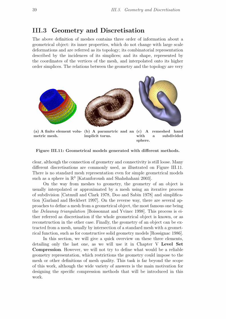
III.3 Geometry and DiscretisationThe above definition of meshes contains three order of information about ageometrical object: its inner properties, which do not change with large scaledeformations and are referred as its topology; its combinatorial representationdescribed by the incidences of its simplices; and its shape, represented bythe coordinates of the vertices of the mesh, and interpolated onto its higherorder simplices. The relations between the geometry and the topology are very

(a) A finite element volu-metric mesh.

(b) A paramrtric and animplicit torus.

(c) A remeshed handwith a subdividedsphere.

Figure III.11: Geometrical models generated with different methods.

clear, although the connection of geometry and connectivity is still loose. Manydifferent discretisations are commonly used, as illustrated on Figure III.11.There is no standard mesh representation even for simple geometrical modelssuch as a sphere in R3 [Katanforoush and Shahshahani 2003].

On the way from meshes to geometry, the geometry of an object isusually interpolated or approximated by a mesh using an iterative processof subdivision [Catmull and Clark 1978, Doo and Sabin 1978] and simplifica-tion [Garland and Heckbert 1997]. On the reverse way, there are several ap-proaches to define a mesh from a geometrical object, the most famous one beingthe Delaunay triangulation [Boissonnat and Yvinec 1998]. This process is ei-ther referred as discretisation if the whole geometrical object is known, or asreconstruction in the other case. Finally, the geometry of an object can be ex-tracted from a mesh, usually by intersection of a standard mesh with a geomet-rical function, such as for constructive solid geometry models [Rossignac 1986].

In this section, we will give a quick overview on these three elements,detailing only the last one, as we will use it in Chapter V Level SetCompression. However, we will not try to define what would be a reliablegeometry representation, which restrictions the geometry could impose to themesh or other definitions of mesh quality. This task is far beyond the scopeof this work, although the wide variety of answers is the main motivation fordesigning the specific compression methods that will be introduced in thiswork.

Chapter III. Meshes and Geometry 40

(a) Subdivision and Smoothing

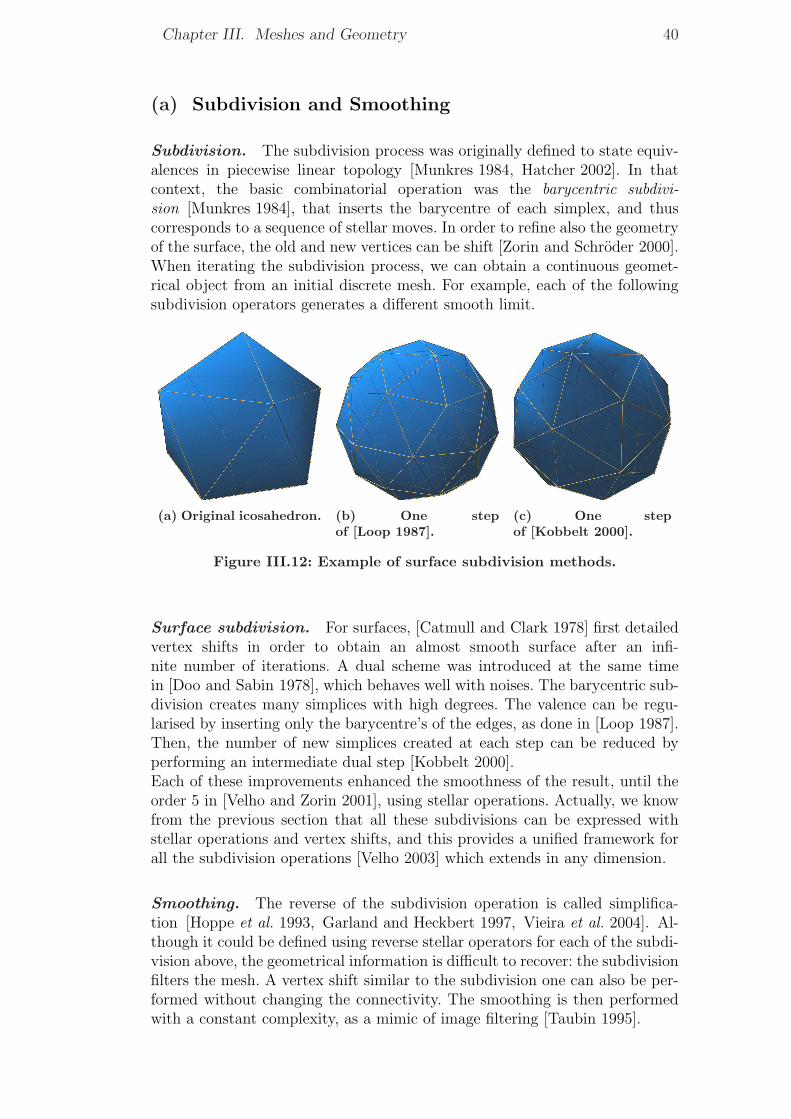
Subdivision. The subdivision process was originally defined to state equiv-alences in piecewise linear topology [Munkres 1984, Hatcher 2002]. In thatcontext, the basic combinatorial operation was the barycentric subdivi-sion [Munkres 1984], that inserts the barycentre of each simplex, and thuscorresponds to a sequence of stellar moves. In order to refine also the geometryof the surface, the old and new vertices can be shift [Zorin and Schroder 2000].When iterating the subdivision process, we can obtain a continuous geomet-rical object from an initial discrete mesh. For example, each of the followingsubdivision operators generates a different smooth limit.

(a) Original icosahedron. (b) One stepof [Loop 1987].

(c) One stepof [Kobbelt 2000].

Figure III.12: Example of surface subdivision methods.

Surface subdivision. For surfaces, [Catmull and Clark 1978] first detailedvertex shifts in order to obtain an almost smooth surface after an infi-nite number of iterations. A dual scheme was introduced at the same timein [Doo and Sabin 1978], which behaves well with noises. The barycentric sub-division creates many simplices with high degrees. The valence can be regu-larised by inserting only the barycentre’s of the edges, as done in [Loop 1987].Then, the number of new simplices created at each step can be reduced byperforming an intermediate dual step [Kobbelt 2000].Each of these improvements enhanced the smoothness of the result, until theorder 5 in [Velho and Zorin 2001], using stellar operations. Actually, we knowfrom the previous section that all these subdivisions can be expressed withstellar operations and vertex shifts, and this provides a unified framework forall the subdivision operations [Velho 2003] which extends in any dimension.

Smoothing. The reverse of the subdivision operation is called simplifica-tion [Hoppe et al. 1993, Garland and Heckbert 1997, Vieira et al. 2004]. Al-though it could be defined using reverse stellar operators for each of the subdi-vision above, the geometrical information is difficult to recover: the subdivisionfilters the mesh. A vertex shift similar to the subdivision one can also be per-formed without changing the connectivity. The smoothing is then performedwith a constant complexity, as a mimic of image filtering [Taubin 1995].

41 III.3. Geometry and Discretisation

These filters are very useful for practical cases, especially to enhance meshesresulting from noisy acquisition [Fleishman et al. 2003] or lossy transmis-sion [Desbrun et al. 1999, Taubin 1999], as in Chapter V Level Set Com-pression.

(b) Delaunay Triangulation

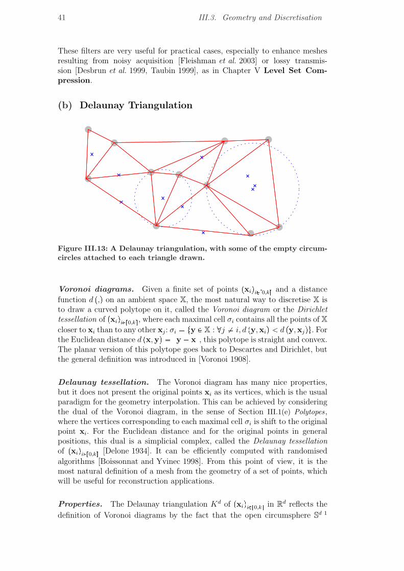
Figure III.13: A Delaunay triangulation, with some of the empty circum-circles attached to each triangle drawn.

Voronoi diagrams. Given a finite set of points pxiqiPv0,kw and a distance

function d p,q on an ambient space X, the most natural way to discretise X isto draw a curved polytope on it, called the Voronoi diagram or the Dirichlettessellation of pxiqiPv0,kw, where each maximal cell σi contains all the points of Xcloser to xi than to any other xj: σi � ty P X : @j � i, d py,xiq   d py,xjqu. Forthe Euclidean distance d px,yq � }y � x}, this polytope is straight and convex.The planar version of this polytope goes back to Descartes and Dirichlet, butthe general definition was introduced in [Voronoi 1908].

Delaunay tessellation. The Voronoi diagram has many nice properties,but it does not present the original points xi as its vertices, which is the usualparadigm for the geometry interpolation. This can be achieved by consideringthe dual of the Voronoi diagram, in the sense of Section III.1(e) Polytopes,where the vertices corresponding to each maximal cell σi is shift to the originalpoint xi. For the Euclidean distance and for the original points in generalpositions, this dual is a simplicial complex, called the Delaunay tessellationof pxiqiPv0,kw [Delone 1934]. It can be efficiently computed with randomised

algorithms [Boissonnat and Yvinec 1998]. From this point of view, it is themost natural definition of a mesh from the geometry of a set of points, whichwill be useful for reconstruction applications.

Properties. The Delaunay triangulation Kd of pxiqiPv0,kw in Rd reflects the

definition of Voronoi diagrams by the fact that the open circumsphere Sd�1

Chapter III. Meshes and Geometry 42

of any maximal simplex is always empty. Moreover, the union of all compactsimplices in the triangulation is the convex hull of the original points. For theEuclidean distance, Delaunay triangulations maximise the minimum internalangle of its simplices [Boissonnat and Yvinec 1998]. These properties are usefulfor packing problems and for differential approximations, since the asymptoticaccuracy of derivative estimators is usually related to the angle of the elementsof the mesh. Moreover, it relates directly to sampling conditions on thegeometry of smooth and non–smooth objects [Boissonnat and Oudot 2005].

Delaunay–based reconstruction. The above properties make Delau-nay triangulations a very significant choice for reconstruction algorithms,from slice interpolation [Boissonnat and Geiger 1993, Lopes et al. 2000,Nonato et al. 2005] to spatial restriction [Chaine and Bouakaz 2000,Boissonnat and Cazals 2002] and greedy traversal [Bernardini et al. 1999,Cohen–Steiner and Da 2002] inside the Delaunay triangulation and furthermore complex methods [Amenta and Kullori 2002]. These methods deduce amesh from a set of points in a deterministic manner, which can be used as abasis for decompressing a mesh knowing its vertices.

Ball pivoting algorithm. In Chapter VI GEncode, we will prefer greedyapproaches in order to control the decompression on the fly. Particularly,the Ball Pivoting algorithm of [Bernardini et al. 1999] will serve as the basicexample. This algorithm creates an initial triangle, a priori the triangle withthe smallest possible circumradius for the given point set, and then recursivelyattach the triangle with the smallest possible circumradius to the boundaryof the mesh being reconstructed. The original algorithm put a threshold onthe circumradius of the inserted triangle, in order to allow reconstructingopen surfaces. It can be directly implemented with the Handle operatorsof Section III.2(b) Handle Operators, as described in [Medeiros et al. 2003,Medeiros et al. 2004]. The reconstructed surface is then a subcomplex of thevolumetric Delaunay triangulation.

(c) Multi–Triangulations

Order of triangulations. In theory, a geometrical model can be approxi-mated by a sequence of subdivisions on an original, coarse mesh. In practise,the size of the mesh must remain reasonable to be handled by a computer,but this sequence of subdivisions still generates a refinement of the resolutionof the geometry. We will formalise the fact that a complex K 1 is obtained bysubdivision from K by a hierarchical relation: K ¶ K 1.Actually, these subdivisions can be adapted to refine only a part of a mesh,for example by stellar operations in a specified neighbourhood [Velho 2004]or by inserting points in the Delaunay triangulation [Devillers 2002]. Depend-ing on the neighbourhood chosen, these subdivisions will generate differentmeshes, and the order ¶ is thus only a partial order. The hierarchy generatedby ¶ is called a multi–triangulation [de Floriani et al. 1997, Puppo 1998].

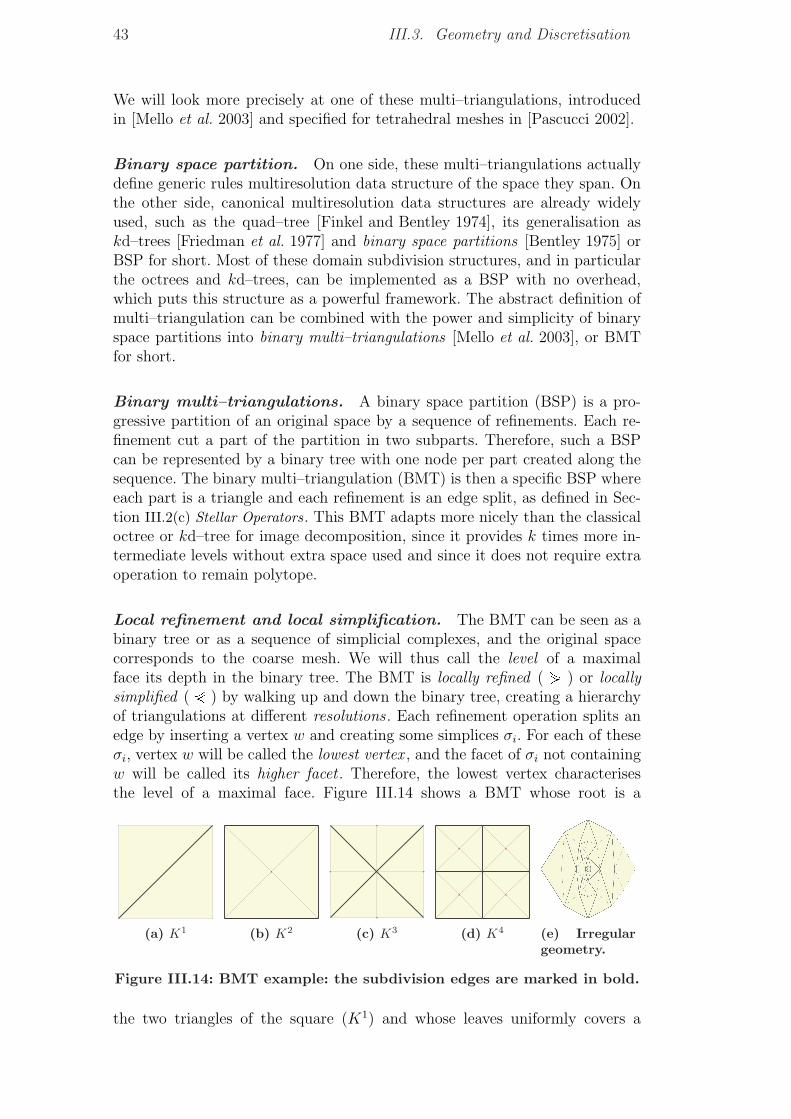
43 III.3. Geometry and Discretisation

We will look more precisely at one of these multi–triangulations, introducedin [Mello et al. 2003] and specified for tetrahedral meshes in [Pascucci 2002].

Binary space partition. On one side, these multi–triangulations actuallydefine generic rules multiresolution data structure of the space they span. Onthe other side, canonical multiresolution data structures are already widelyused, such as the quad–tree [Finkel and Bentley 1974], its generalisation askd–trees [Friedman et al. 1977] and binary space partitions [Bentley 1975] orBSP for short. Most of these domain subdivision structures, and in particularthe octrees and kd–trees, can be implemented as a BSP with no overhead,which puts this structure as a powerful framework. The abstract definition ofmulti–triangulation can be combined with the power and simplicity of binaryspace partitions into binary multi–triangulations [Mello et al. 2003], or BMTfor short.

Binary multi–triangulations. A binary space partition (BSP) is a pro-gressive partition of an original space by a sequence of refinements. Each re-finement cut a part of the partition in two subparts. Therefore, such a BSPcan be represented by a binary tree with one node per part created along thesequence. The binary multi–triangulation (BMT) is then a specific BSP whereeach part is a triangle and each refinement is an edge split, as defined in Sec-tion III.2(c) Stellar Operators. This BMT adapts more nicely than the classicaloctree or kd–tree for image decomposition, since it provides k times more in-termediate levels without extra space used and since it does not require extraoperation to remain polytope.

Local refinement and local simplification. The BMT can be seen as abinary tree or as a sequence of simplicial complexes, and the original spacecorresponds to the coarse mesh. We will thus call the level of a maximalface its depth in the binary tree. The BMT is locally refined ( · ) or locallysimplified ( ¶ ) by walking up and down the binary tree, creating a hierarchyof triangulations at different resolutions . Each refinement operation splits anedge by inserting a vertex w and creating some simplices σi. For each of theseσi, vertex w will be called the lowest vertex , and the facet of σi not containingw will be called its higher facet . Therefore, the lowest vertex characterisesthe level of a maximal face. Figure III.14 shows a BMT whose root is a

(a) K1 (b) K2 (c) K3 (d) K4 (e) Irregulargeometry.

Figure III.14: BMT example: the subdivision edges are marked in bold.

the two triangles of the square (K1) and whose leaves uniformly covers a

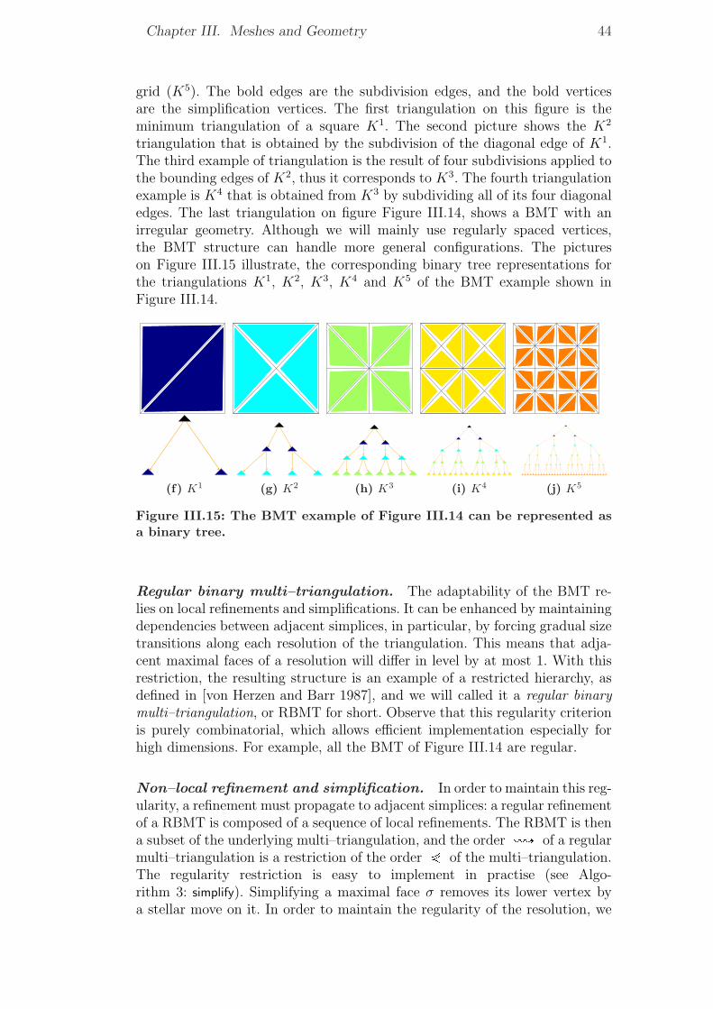
Chapter III. Meshes and Geometry 44

grid (K5). The bold edges are the subdivision edges, and the bold verticesare the simplification vertices. The first triangulation on this figure is theminimum triangulation of a square K1. The second picture shows the K2

triangulation that is obtained by the subdivision of the diagonal edge of K1.The third example of triangulation is the result of four subdivisions applied tothe bounding edges of K2, thus it corresponds to K3. The fourth triangulationexample is K4 that is obtained from K3 by subdividing all of its four diagonaledges. The last triangulation on figure Figure III.14, shows a BMT with anirregular geometry. Although we will mainly use regularly spaced vertices,the BMT structure can handle more general configurations. The pictureson Figure III.15 illustrate, the corresponding binary tree representations forthe triangulations K1, K2, K3, K4 and K5 of the BMT example shown inFigure III.14.

(f) K1 (g) K2 (h) K3 (i) K4 (j) K5

Figure III.15: The BMT example of Figure III.14 can be represented asa binary tree.

Regular binary multi–triangulation. The adaptability of the BMT re-lies on local refinements and simplifications. It can be enhanced by maintainingdependencies between adjacent simplices, in particular, by forcing gradual sizetransitions along each resolution of the triangulation. This means that adja-cent maximal faces of a resolution will differ in level by at most 1. With thisrestriction, the resulting structure is an example of a restricted hierarchy, asdefined in [von Herzen and Barr 1987], and we will called it a regular binarymulti–triangulation, or RBMT for short. Observe that this regularity criterionis purely combinatorial, which allows efficient implementation especially forhigh dimensions. For example, all the BMT of Figure III.14 are regular.

Non–local refinement and simplification. In order to maintain this reg-ularity, a refinement must propagate to adjacent simplices: a regular refinementof a RBMT is composed of a sequence of local refinements. The RBMT is thena subset of the underlying multi–triangulation, and the order ù of a regularmulti–triangulation is a restriction of the order ¶ of the multi–triangulation.The regularity restriction is easy to implement in practise (see Algo-rithm 3: simplify). Simplifying a maximal face σ removes its lower vertex bya stellar move on it. In order to maintain the regularity of the resolution, we

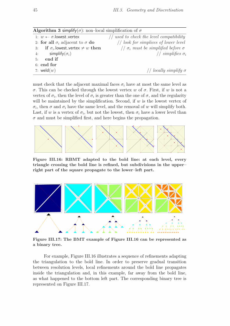
45 III.3. Geometry and Discretisation

Algorithm 3 simplify(σ): non–local simplification of σ

1: w Ð σ.lowest vertex // used to check the level compatibility2: for all σi adjacent to σ do // look for simplices of lower level3: if σi.lowest vertex � w then // σi must be simplified before σ4: simplify(σi) // simplifies σi

5: end if6: end for7: weld(w) // locally simplify σ

must check that the adjacent maximal faces σi have at most the same level asσ. This can be checked through the lowest vertex w of σ. First, if w is not avertex of σi, then the level of σi is greater than the one of σ, and the regularitywill be maintained by the simplification. Second, if w is the lowest vertex ofσi, then σ and σi have the same level, and the removal of w will simplify both.Last, if w is a vertex of σi, but not the lowest, then σi have a lower level thanσ and must be simplified first, and here begins the propagation.

Figure III.16: RBMT adapted to the bold line: at each level, everytriangle crossing the bold line is refined, but subdivisions in the upper–right part of the square propagate to the lower–left part.

Figure III.17: The BMT example of Figure III.16 can be represented asa binary tree.

For example, Figure III.16 illustrates a sequence of refinements adaptingthe triangulation to the bold line. In order to preserve gradual transitionbetween resolution levels, local refinements around the bold line propagatesinside the triangulation and, in this example, far away from the bold line,as what happened to the bottom left part. The corresponding binary tree isrepresented on Figure III.17.

IVConnectivity–Driven Compression

This work aims at compressing geometrical objects represented by meshes.Since there is still no strong relation between the geometry and the connectivityof these meshes for the usual objects considered by graphics applications,dedicated compression schemes consider either that the common informationcan be deduced from either the connectivity or the geometry. The first optionassumes that the star of a simplex has a simple geometry, which can bewell approximated by simple methods such as linear interpolation. Then,the geometry can be efficiently encoded by a connectivity traversal of themesh, leading to connectivity–driven compression schemes. The second optionpredicts the connectivity from the geometry, and will be referred as geometry–driven compression schemes. In that case, the connectivity is usually bettercompressed, but it needs efficient coding of the geometry.

In this chapter, we will focus on the connectivity part of the compres-sion, in order to clarify the position of geometry–driven compression of thenext chapters. These connectivity–driven methods improved so much in thelast decade that the compression ratio for usual surface connectivity turnsaround 2/3 bits per vertex. We will give a general framework for handlingthe critical elements of the connectivity: the topological singularities. Thesesingularities are well understood for surfaces through the Handle operatorsof Section III.2(b) Handle Operators. We will then focus on the Edgebreakerscheme, and introduce two new improvements: the handling of boundary, asa consequence of this framework for singularities, and a small improvement ofthe decompression algorithm. We will conclude this chapter with compressionratios of the Edgebreaker on usual models with our improvements, and we willdetail the specificities of connectivity–driven compression scheme. The goalof this chapter is to state what connectivity–driven compression means, withthe detailed example of the Edgebreaker (Figure IV.1 and Figure IV.2), and toshow where these algorithms are well suited.

IV.1 PrinciplesConnectivity–driven compression schemes rely on a traversal of the mesh inorder to visit each vertex, and to identify it on further visits. This way, thegeometry of the vertex needs to be transmitted only once, and the traver-sal encodes the connectivity of the mesh. This general framework suits par-ticularly well for manifold polytopes. Most of the existing compression tech-niques are dedicated to surfaces, and we will focus on these algorithms. Fur-ther extensions to non–manifold cases are described in [Gueziec et al. 1998],

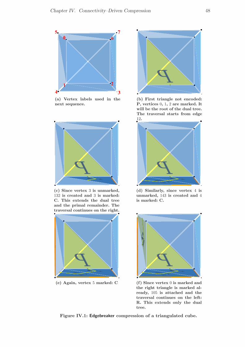
Chapter IV. Connectivity–Driven Compression 48

(a) Vertex labels used in thenext sequence.

(b) First triangle not encoded:P, vertices 0, 1, 2 are marked. Itwill be the root of the dual tree.The traversal starts from edge12.

(c) Since vertex 3 is unmarked,132 is created and 3 is marked:C. This extends the dual treeand the primal remainder. Thetraversal continues on the right.

(d) Similarly, since vertex 4 isunmarked, 143 is created and 4is marked: C.

(e) Again, vertex 5 marked: C (f) Since vertex 0 is marked andthe right triangle is marked al-ready, 105 is attached and thetraversal continues on the left:R. This extends only the dualtree.

Figure IV.1: Edgebreaker compression of a triangulated cube.

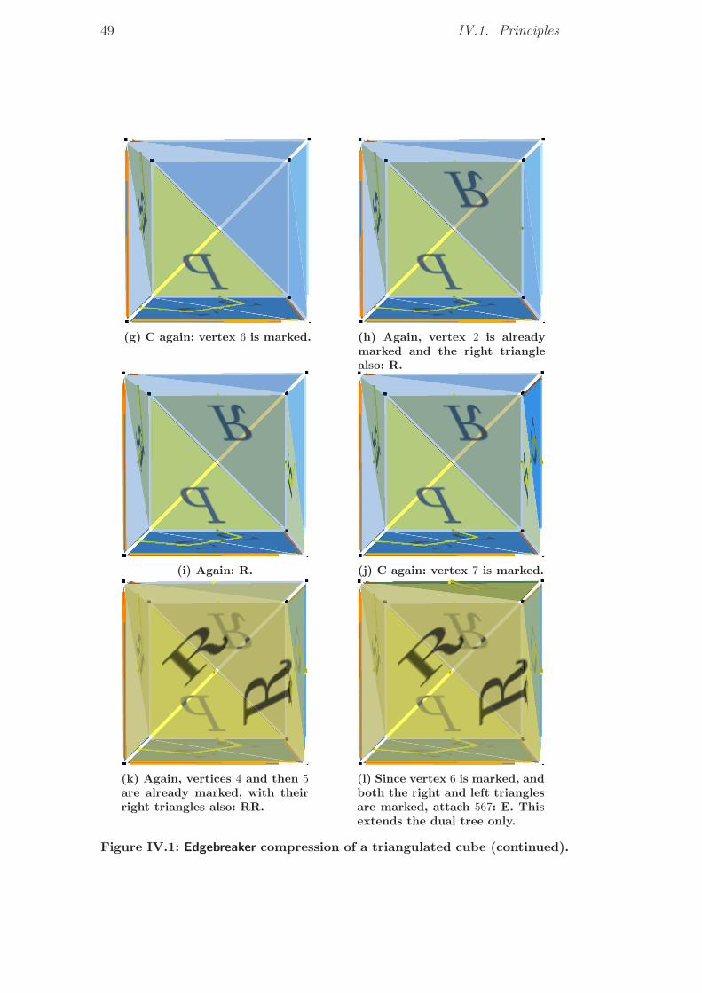
49 IV.1. Principles

(g) C again: vertex 6 is marked. (h) Again, vertex 2 is alreadymarked and the right trianglealso: R.

(i) Again: R. (j) C again: vertex 7 is marked.

(k) Again, vertices 4 and then 5are already marked, with theirright triangles also: RR.

(l) Since vertex 6 is marked, andboth the right and left trianglesare marked, attach 567: E. Thisextends the dual tree only.

Figure IV.1: Edgebreaker compression of a triangulated cube (continued).

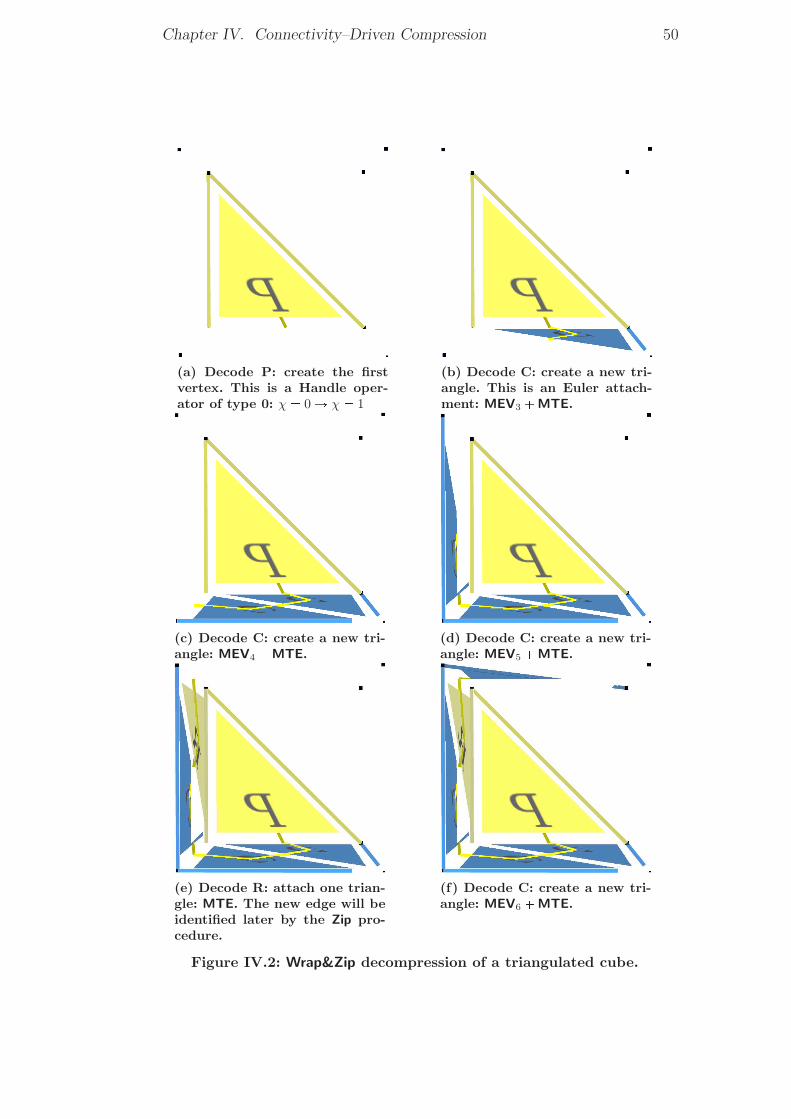
Chapter IV. Connectivity–Driven Compression 50

(a) Decode P: create the firstvertex. This is a Handle oper-ator of type 0: χ � 0Ñ χ � 1

(b) Decode C: create a new tri-angle. This is an Euler attach-ment: MEV3 �MTE.

(c) Decode C: create a new tri-angle: MEV4 �MTE.

(d) Decode C: create a new tri-angle: MEV5 �MTE.

(e) Decode R: attach one trian-gle: MTE. The new edge will beidentified later by the Zip pro-cedure.

(f) Decode C: create a new tri-angle: MEV6 �MTE.

Figure IV.2: Wrap&Zip decompression of a triangulated cube.

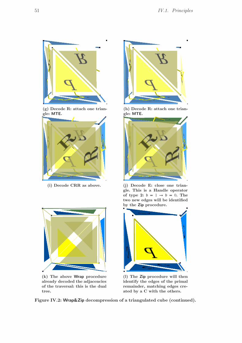
51 IV.1. Principles

(g) Decode R: attach one trian-gle: MTE.

(h) Decode R: attach one trian-gle: MTE.

(i) Decode CRR as above. (j) Decode E: close one trian-gle. This is a Handle operatorof type 2: b � 1 Ñ b � 0. Thetwo new edges will be identifiedby the Zip procedure.

(k) The above Wrap procedurealready decoded the adjacenciesof the traversal: this is the dualtree.

(l) The Zip procedure will thenidentify the edges of the primalremainder, matching edges cre-ated by a C with the others.

Figure IV.2: Wrap&Zip decompression of a triangulated cube (continued).

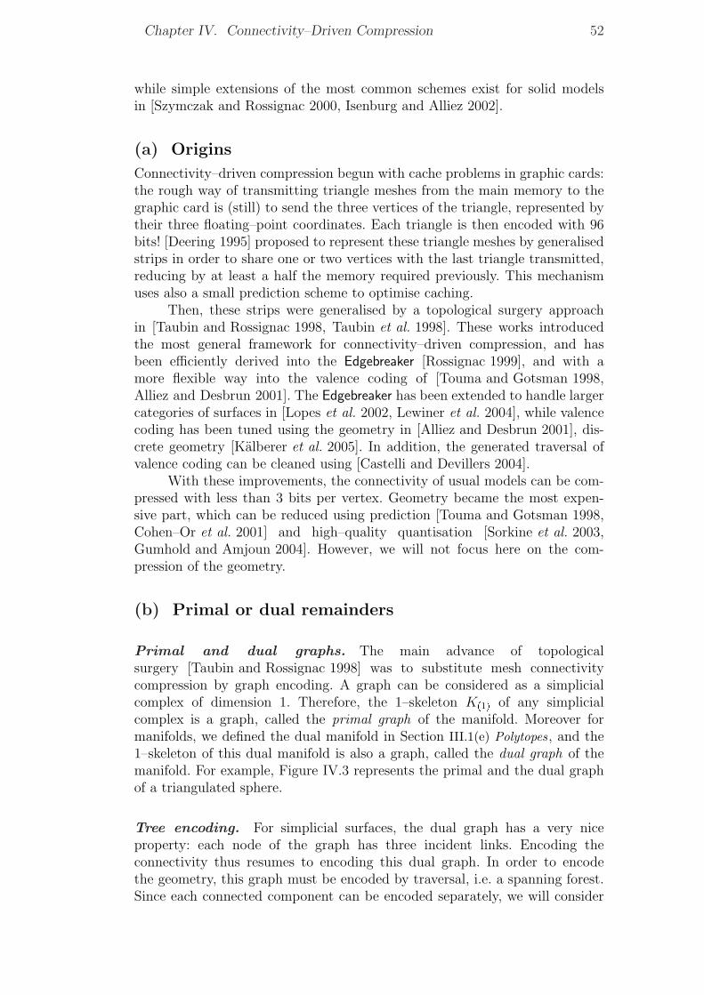
Chapter IV. Connectivity–Driven Compression 52

while simple extensions of the most common schemes exist for solid modelsin [Szymczak and Rossignac 2000, Isenburg and Alliez 2002].

(a) Origins

Connectivity–driven compression begun with cache problems in graphic cards:the rough way of transmitting triangle meshes from the main memory to thegraphic card is (still) to send the three vertices of the triangle, represented bytheir three floating–point coordinates. Each triangle is then encoded with 96bits! [Deering 1995] proposed to represent these triangle meshes by generalisedstrips in order to share one or two vertices with the last triangle transmitted,reducing by at least a half the memory required previously. This mechanismuses also a small prediction scheme to optimise caching.

Then, these strips were generalised by a topological surgery approachin [Taubin and Rossignac 1998, Taubin et al. 1998]. These works introducedthe most general framework for connectivity–driven compression, and hasbeen efficiently derived into the Edgebreaker [Rossignac 1999], and with amore flexible way into the valence coding of [Touma and Gotsman 1998,Alliez and Desbrun 2001]. The Edgebreaker has been extended to handle largercategories of surfaces in [Lopes et al. 2002, Lewiner et al. 2004], while valencecoding has been tuned using the geometry in [Alliez and Desbrun 2001], dis-crete geometry [Kalberer et al. 2005]. In addition, the generated traversal ofvalence coding can be cleaned using [Castelli and Devillers 2004].

With these improvements, the connectivity of usual models can be com-pressed with less than 3 bits per vertex. Geometry became the most expen-sive part, which can be reduced using prediction [Touma and Gotsman 1998,Cohen–Or et al. 2001] and high–quality quantisation [Sorkine et al. 2003,Gumhold and Amjoun 2004]. However, we will not focus here on the com-pression of the geometry.

(b) Primal or dual remainders

Primal and dual graphs. The main advance of topologicalsurgery [Taubin and Rossignac 1998] was to substitute mesh connectivitycompression by graph encoding. A graph can be considered as a simplicialcomplex of dimension 1. Therefore, the 1–skeleton Kp1q of any simplicialcomplex is a graph, called the primal graph of the manifold. Moreover formanifolds, we defined the dual manifold in Section III.1(e) Polytopes, and the1–skeleton of this dual manifold is also a graph, called the dual graph of themanifold. For example, Figure IV.3 represents the primal and the dual graphof a triangulated sphere.

Tree encoding. For simplicial surfaces, the dual graph has a very niceproperty: each node of the graph has three incident links. Encoding theconnectivity thus resumes to encoding this dual graph. In order to encodethe geometry, this graph must be encoded by traversal, i.e. a spanning forest.Since each connected component can be encoded separately, we will consider

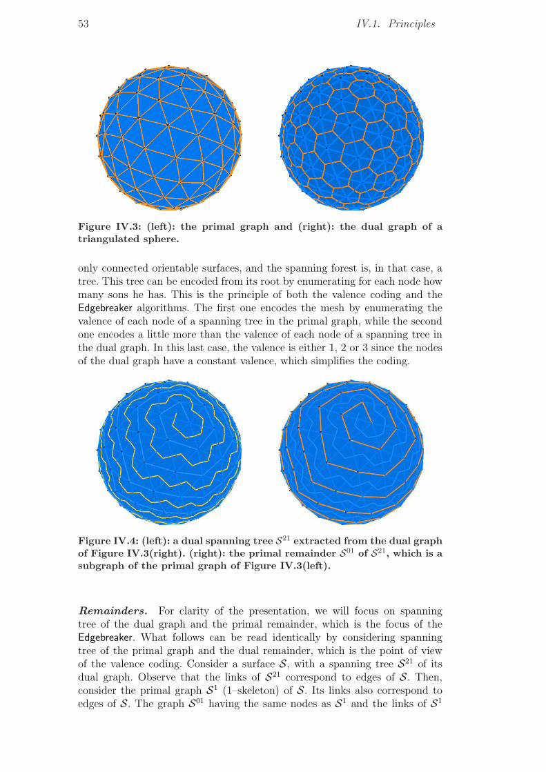
53 IV.1. Principles

Figure IV.3: (left): the primal graph and (right): the dual graph of atriangulated sphere.

only connected orientable surfaces, and the spanning forest is, in that case, atree. This tree can be encoded from its root by enumerating for each node howmany sons he has. This is the principle of both the valence coding and theEdgebreaker algorithms. The first one encodes the mesh by enumerating thevalence of each node of a spanning tree in the primal graph, while the secondone encodes a little more than the valence of each node of a spanning tree inthe dual graph. In this last case, the valence is either 1, 2 or 3 since the nodesof the dual graph have a constant valence, which simplifies the coding.

Figure IV.4: (left): a dual spanning tree S21 extracted from the dual graphof Figure IV.3(right). (right): the primal remainder S01 of S21, which is asubgraph of the primal graph of Figure IV.3(left).

Remainders. For clarity of the presentation, we will focus on spanningtree of the dual graph and the primal remainder, which is the focus of theEdgebreaker. What follows can be read identically by considering spanningtree of the primal graph and the dual remainder, which is the point of viewof the valence coding. Consider a surface S, with a spanning tree S21 of itsdual graph. Observe that the links of S21 correspond to edges of S. Then,consider the primal graph S1 (1–skeleton) of S. Its links also correspond toedges of S. The graph S01 having the same nodes as S1 and the links of S1

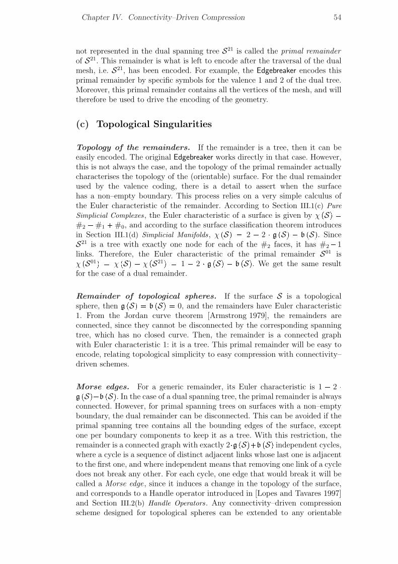
Chapter IV. Connectivity–Driven Compression 54

not represented in the dual spanning tree S21 is called the primal remainderof S21. This remainder is what is left to encode after the traversal of the dualmesh, i.e. S21, has been encoded. For example, the Edgebreaker encodes thisprimal remainder by specific symbols for the valence 1 and 2 of the dual tree.Moreover, this primal remainder contains all the vertices of the mesh, and willtherefore be used to drive the encoding of the geometry.

(c) Topological Singularities

Topology of the remainders. If the remainder is a tree, then it can beeasily encoded. The original Edgebreaker works directly in that case. However,this is not always the case, and the topology of the primal remainder actuallycharacterises the topology of the (orientable) surface. For the dual remainderused by the valence coding, there is a detail to assert when the surfacehas a non–empty boundary. This process relies on a very simple calculus ofthe Euler characteristic of the remainder. According to Section III.1(c) PureSimplicial Complexes, the Euler characteristic of a surface is given by χ pSq �#2 �#1 �#0, and according to the surface classification theorem introducesin Section III.1(d) Simplicial Manifolds, χ pSq � 2 � 2 � g pSq � b pSq. SinceS21 is a tree with exactly one node for each of the #2 faces, it has #2�1links. Therefore, the Euler characteristic of the primal remainder S01 isχ pS01q � χ pSq � χ pS21q � 1 � 2 � g pSq � b pSq. We get the same resultfor the case of a dual remainder.

Remainder of topological spheres. If the surface S is a topologicalsphere, then g pSq � b pSq � 0, and the remainders have Euler characteristic1. From the Jordan curve theorem [Armstrong 1979], the remainders areconnected, since they cannot be disconnected by the corresponding spanningtree, which has no closed curve. Then, the remainder is a connected graphwith Euler characteristic 1: it is a tree. This primal remainder will be easy toencode, relating topological simplicity to easy compression with connectivity–driven schemes.

Morse edges. For a generic remainder, its Euler characteristic is 1 � 2 �g pSq�b pSq. In the case of a dual spanning tree, the primal remainder is alwaysconnected. However, for primal spanning trees on surfaces with a non–emptyboundary, the dual remainder can be disconnected. This can be avoided if theprimal spanning tree contains all the bounding edges of the surface, exceptone per boundary components to keep it as a tree. With this restriction, theremainder is a connected graph with exactly 2�g pSq�b pSq independent cycles,where a cycle is a sequence of distinct adjacent links whose last one is adjacentto the first one, and where independent means that removing one link of a cycledoes not break any other. For each cycle, one edge that would break it will becalled a Morse edge, since it induces a change in the topology of the surface,and corresponds to a Handle operator introduced in [Lopes and Tavares 1997]and Section III.2(b) Handle Operators. Any connectivity–driven compressionscheme designed for topological spheres can be extended to any orientable

55 IV.2. The Edgebreaker example

surface by encoding separately these Morse edges. For example, in the case of

Figure IV.5: (left): a primal remainder on a torus (genus 1): the topmostand bottommost horizontal edges are identified, and so do the leftmostand rightmost ones. (right) a primal remainder on an annulus (twobounding curves).

a sphere, the primal remainder is a tree, as shown on Figure IV.4. For a meshwith genus one or with two boundary curves, the primal remainder is a graphwith two cycles, as shown on Figure IV.5.

IV.2 The Edgebreaker exampleThe Edgebreaker scheme has been enhanced and adapted from the Topologi-cal Surgery [Taubin and Rossignac 1998] to yield an efficient but initially re-stricted algorithm [Rossignac 1999], which encodes the connectivity of anysimplicial surface homeomorphic to a sphere with a guaranteed worst casecode of 1.83 bits per triangle [King and Rossignac 1999]. The Wrap&Zip al-gorithm introduced in [Rossignac and Szymczak 1999] enhanced the originalEdgebreaker decompression worst–case complexity from O pn2q to O pnq, wheren is the number of triangles of the mesh. It decompresses the mesh in twopasses, a direct and a recursive one. It is possible to decompress it in onlyone pass using the Spirale Reversi algorithm of [Isenburg and Snoeyink 2000],but it requires to read the encoded backwards, which is not appropriate forthe Huffman encoding of [King and Rossignac 1999] or the arithmetic en-coding. But the true value of Edgebreaker lies in the efficiency and in thesimplicity of its implementations [Rossignac et al. 2001], which is very con-cise. This simple algorithm has been extended to deal with non–simplicialsurfaces [Kronrod and Gotsman 2001] and the compression of simplicial sur-faces with handles has been enhanced in [Lopes et al. 2003] using handle data.Because of its simplicity, Edgebreaker is viewed as the emerging standardfor 3D compression [Salomon 2000] and may provide an alternative for thecurrent MPEG–4 standard, which is based on the Topological Surgery ap-proach [Taubin and Rossignac 1998].

In this section, we will enhance the Edgebreaker compression for surfaceswith a non–empty boundary. [King and Rossignac 1999] encoded these sur-

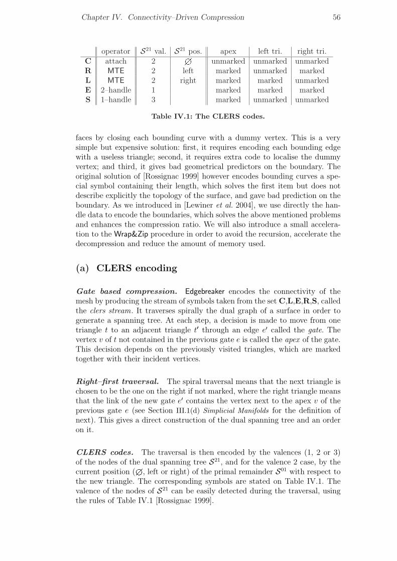
Chapter IV. Connectivity–Driven Compression 56

operator S21 val. S21 pos. apex left tri. right tri.C attach 2 H unmarked unmarked unmarkedR MTE 2 left marked unmarked markedL MTE 2 right marked marked unmarkedE 2–handle 1 marked marked markedS 1–handle 3 marked unmarked unmarked

Table IV.1: The CLERS codes.

faces by closing each bounding curve with a dummy vertex. This is a verysimple but expensive solution: first, it requires encoding each bounding edgewith a useless triangle; second, it requires extra code to localise the dummyvertex; and third, it gives bad geometrical predictors on the boundary. Theoriginal solution of [Rossignac 1999] however encodes bounding curves a spe-cial symbol containing their length, which solves the first item but does notdescribe explicitly the topology of the surface, and gave bad prediction on theboundary. As we introduced in [Lewiner et al. 2004], we use directly the han-dle data to encode the boundaries, which solves the above mentioned problemsand enhances the compression ratio. We will also introduce a small accelera-tion to the Wrap&Zip procedure in order to avoid the recursion, accelerate thedecompression and reduce the amount of memory used.

(a) CLERS encoding

Gate based compression. Edgebreaker encodes the connectivity of themesh by producing the stream of symbols taken from the set C,L,E,R,S, calledthe clers stream. It traverses spirally the dual graph of a surface in order togenerate a spanning tree. At each step, a decision is made to move from onetriangle t to an adjacent triangle t1 through an edge e1 called the gate. Thevertex v of t not contained in the previous gate e is called the apex of the gate.This decision depends on the previously visited triangles, which are markedtogether with their incident vertices.

Right–first traversal. The spiral traversal means that the next triangle ischosen to be the one on the right if not marked, where the right triangle meansthat the link of the new gate e1 contains the vertex next to the apex v of theprevious gate e (see Section III.1(d) Simplicial Manifolds for the definition ofnext). This gives a direct construction of the dual spanning tree and an orderon it.

CLERS codes. The traversal is then encoded by the valences (1, 2 or 3)of the nodes of the dual spanning tree S21, and for the valence 2 case, by thecurrent position (H, left or right) of the primal remainder S01 with respect tothe new triangle. The corresponding symbols are stated on Table IV.1. Thevalence of the nodes of S21 can be easily detected during the traversal, usingthe rules of Table IV.1 [Rossignac 1999].

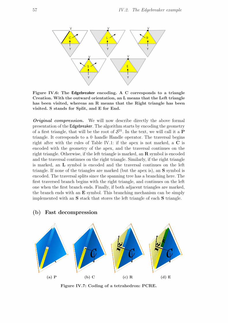
57 IV.2. The Edgebreaker example

Figure IV.6: The Edgebreaker encoding. A C corresponds to a triangleCreation. With the outward orientation, an L means that the Left trianglehas been visited, whereas an R means that the Right triangle has beenvisited. S stands for Split, and E for End.

Original compression. We will now describe directly the above formalpresentation of the Edgebreaker. The algorithm starts by encoding the geometryof a first triangle, that will be the root of S21. In the text, we will call it a Ptriangle. It corresponds to a 0–handle Handle operator. The traversal beginsright after with the rules of Table IV.1: if the apex is not marked, a C isencoded with the geometry of the apex, and the traversal continues on theright triangle. Otherwise, if the left triangle is marked, an R symbol is encodedand the traversal continues on the right triangle. Similarly, if the right triangleis marked, an L symbol is encoded and the traversal continues on the lefttriangle. If none of the triangles are marked (but the apex is), an S symbol isencoded. The traversal splits since the spanning tree has a branching here. Thefirst traversed branch begins with the right triangle, and continues on the leftone when the first branch ends. Finally, if both adjacent triangles are marked,the branch ends with an E symbol. This branching mechanism can be simplyimplemented with an S stack that stores the left triangle of each S triangle.

(b) Fast decompression

(a) P (b) C (c) R (d) E

Figure IV.7: Coding of a tetrahedron: PCRE.

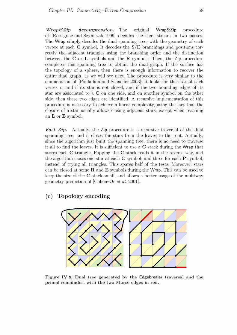
Chapter IV. Connectivity–Driven Compression 58

Wrap&Zip decompression. The original Wrap&Zip procedureof [Rossignac and Szymczak 1999] decodes the clers stream in two passes.The Wrap simply decodes the dual spanning tree, with the geometry of eachvertex at each C symbol. It decodes the S/E branchings and positions cor-rectly the adjacent triangles using the branching order and the distinctionbetween the C or L symbols and the R symbols. Then, the Zip procedurecompletes this spanning tree to obtain the dual graph. If the surface hasthe topology of a sphere, then there is enough information to recover theentire dual graph, as we will see next. The procedure is very similar to theenumeration of [Poulalhon and Schaeffer 2003]: it looks for the star of eachvertex v, and if its star is not closed, and if the two bounding edges of itsstar are associated to a C on one side, and on another symbol on the otherside, then these two edges are identified. A recursive implementation of thisprocedure is necessary to achieve a linear complexity, using the fact that theclosure of a star usually allows closing adjacent stars, except when reachingan L or E symbol.

Fast Zip. Actually, the Zip procedure is a recursive traversal of the dualspanning tree, and it closes the stars from the leaves to the root. Actually,since the algorithm just built the spanning tree, there is no need to traverseit all to find the leaves. It is sufficient to use a C stack during the Wrap thatstores each C triangle. Popping the C stack reads it in the reverse way, andthe algorithm closes one star at each C symbol, and three for each P symbol,instead of trying all triangles. This spares half of the tests. Moreover, starscan be closed at some R and E symbols during the Wrap. This can be used tokeep the size of the C stack small, and allows a better usage of the multiwaygeometry prediction of [Cohen–Or et al. 2001].

(c) Topology encoding

Figure IV.8: Dual tree generated by the Edgebrealer traversal and theprimal remainder, with the two Morse edges in red.

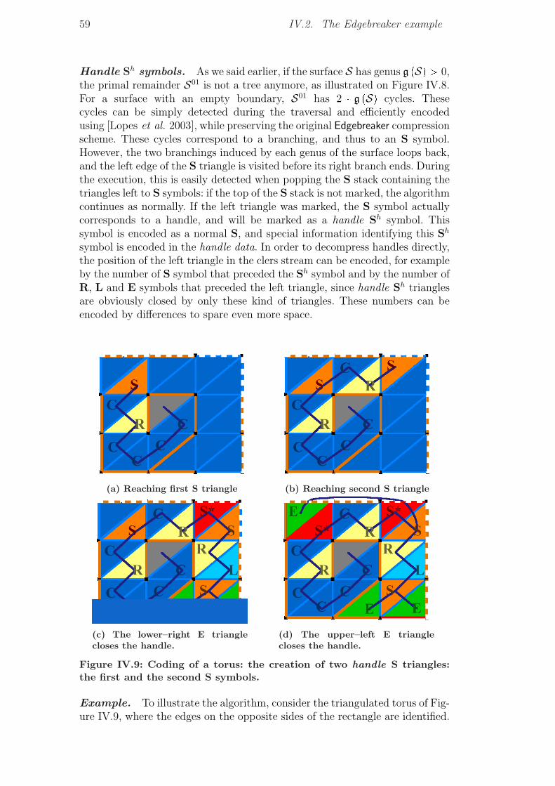
59 IV.2. The Edgebreaker example

Handle Sh symbols. As we said earlier, if the surface S has genus g pSq ¡ 0,the primal remainder S01 is not a tree anymore, as illustrated on Figure IV.8.For a surface with an empty boundary, S01 has 2 � g pSq cycles. Thesecycles can be simply detected during the traversal and efficiently encodedusing [Lopes et al. 2003], while preserving the original Edgebreaker compressionscheme. These cycles correspond to a branching, and thus to an S symbol.However, the two branchings induced by each genus of the surface loops back,and the left edge of the S triangle is visited before its right branch ends. Duringthe execution, this is easily detected when popping the S stack containing thetriangles left to S symbols: if the top of the S stack is not marked, the algorithmcontinues as normally. If the left triangle was marked, the S symbol actuallycorresponds to a handle, and will be marked as a handle Sh symbol. Thissymbol is encoded as a normal S, and special information identifying this Sh

symbol is encoded in the handle data. In order to decompress handles directly,the position of the left triangle in the clers stream can be encoded, for exampleby the number of S symbol that preceded the Sh symbol and by the number ofR, L and E symbols that preceded the left triangle, since handle Sh trianglesare obviously closed by only these kind of triangles. These numbers can beencoded by differences to spare even more space.

(a) Reaching first S triangle (b) Reaching second S triangle

(c) The lower–right E trianglecloses the handle.

(d) The upper–left E trianglecloses the handle.

Figure IV.9: Coding of a torus: the creation of two handle S triangles:the first and the second S symbols.

Example. To illustrate the algorithm, consider the triangulated torus of Fig-ure IV.9, where the edges on the opposite sides of the rectangle are identified.

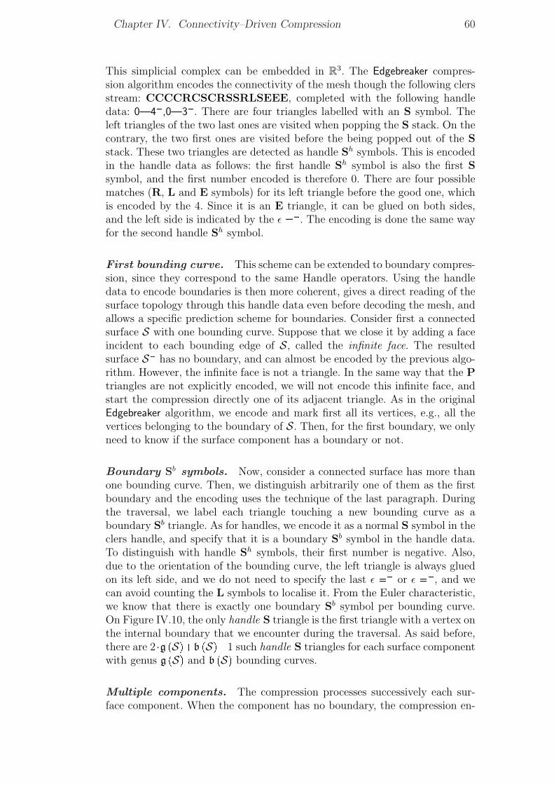
Chapter IV. Connectivity–Driven Compression 60

This simplicial complex can be embedded in R3. The Edgebreaker compres-sion algorithm encodes the connectivity of the mesh though the following clersstream: CCCCRCSCRSSRLSEEE, completed with the following handledata: 0—4�,0—3�. There are four triangles labelled with an S symbol. Theleft triangles of the two last ones are visited when popping the S stack. On thecontrary, the two first ones are visited before the being popped out of the Sstack. These two triangles are detected as handle Sh symbols. This is encodedin the handle data as follows: the first handle Sh symbol is also the first Ssymbol, and the first number encoded is therefore 0. There are four possiblematches (R, L and E symbols) for its left triangle before the good one, whichis encoded by the 4. Since it is an E triangle, it can be glued on both sides,and the left side is indicated by the ε ��. The encoding is done the same wayfor the second handle Sh symbol.

First bounding curve. This scheme can be extended to boundary compres-sion, since they correspond to the same Handle operators. Using the handledata to encode boundaries is then more coherent, gives a direct reading of thesurface topology through this handle data even before decoding the mesh, andallows a specific prediction scheme for boundaries. Consider first a connectedsurface S with one bounding curve. Suppose that we close it by adding a faceincident to each bounding edge of S, called the infinite face. The resultedsurface S� has no boundary, and can almost be encoded by the previous algo-rithm. However, the infinite face is not a triangle. In the same way that the Ptriangles are not explicitly encoded, we will not encode this infinite face, andstart the compression directly one of its adjacent triangle. As in the originalEdgebreaker algorithm, we encode and mark first all its vertices, e.g., all thevertices belonging to the boundary of S. Then, for the first boundary, we onlyneed to know if the surface component has a boundary or not.

Boundary Sb symbols. Now, consider a connected surface has more thanone bounding curve. Then, we distinguish arbitrarily one of them as the firstboundary and the encoding uses the technique of the last paragraph. Duringthe traversal, we label each triangle touching a new bounding curve as aboundary Sb triangle. As for handles, we encode it as a normal S symbol in theclers handle, and specify that it is a boundary Sb symbol in the handle data.To distinguish with handle Sh symbols, their first number is negative. Also,due to the orientation of the bounding curve, the left triangle is always gluedon its left side, and we do not need to specify the last ε �� or ε ��, and wecan avoid counting the L symbols to localise it. From the Euler characteristic,we know that there is exactly one boundary Sb symbol per bounding curve.On Figure IV.10, the only handle S triangle is the first triangle with a vertex onthe internal boundary that we encounter during the traversal. As said before,there are 2�g pSq�b pSq�1 such handle S triangles for each surface componentwith genus g pSq and b pSq bounding curves.

Multiple components. The compression processes successively each sur-face component. When the component has no boundary, the compression en-

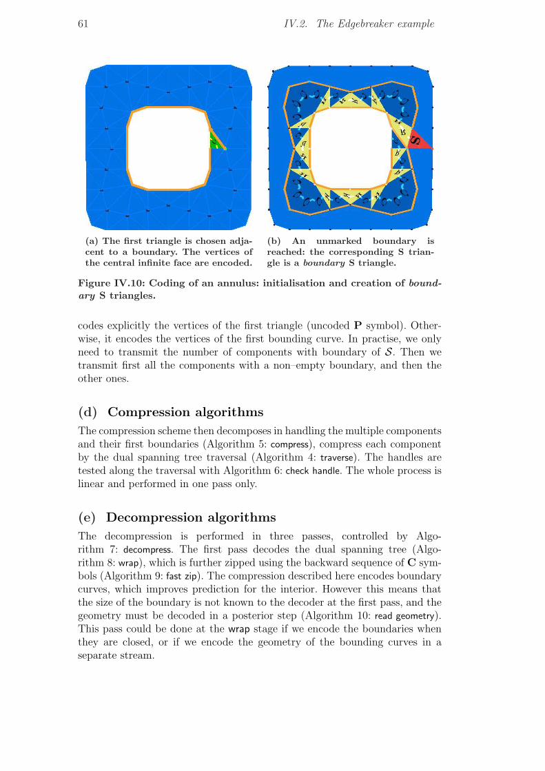
61 IV.2. The Edgebreaker example

(a) The first triangle is chosen adja-cent to a boundary. The vertices ofthe central infinite face are encoded.

(b) An unmarked boundary isreached: the corresponding S trian-gle is a boundary S triangle.

Figure IV.10: Coding of an annulus: initialisation and creation of bound-ary S triangles.

codes explicitly the vertices of the first triangle (uncoded P symbol). Other-wise, it encodes the vertices of the first bounding curve. In practise, we onlyneed to transmit the number of components with boundary of S. Then wetransmit first all the components with a non–empty boundary, and then theother ones.

(d) Compression algorithms

The compression scheme then decomposes in handling the multiple componentsand their first boundaries (Algorithm 5: compress), compress each componentby the dual spanning tree traversal (Algorithm 4: traverse). The handles aretested along the traversal with Algorithm 6: check handle. The whole process islinear and performed in one pass only.

(e) Decompression algorithms

The decompression is performed in three passes, controlled by Algo-rithm 7: decompress. The first pass decodes the dual spanning tree (Algo-rithm 8: wrap), which is further zipped using the backward sequence of C sym-bols (Algorithm 9: fast zip). The compression described here encodes boundarycurves, which improves prediction for the interior. However this means thatthe size of the boundary is not known to the decoder at the first pass, and thegeometry must be decoded in a posterior step (Algorithm 10: read geometry).This pass could be done at the wrap stage if we encode the boundaries whenthey are closed, or if we encode the geometry of the bounding curves in aseparate stream.

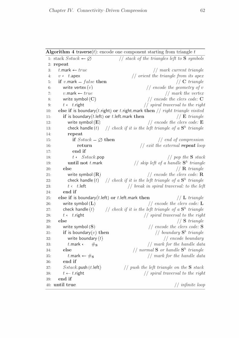
Chapter IV. Connectivity–Driven Compression 62

Algorithm 4 traverse(t): encode one component starting from triangle t

1: stack Sstack ÐH // stack of the triangles left to S symbols2: repeat3: t.mark Ð true // mark current triangle4: v Ð t.apex // orient the triangle from its apex5: if v.mark � false then // C triangle6: write vertex pvq // encode the geometry of v7: v.mark Ð true // mark the vertex8: write symbol pCq // encode the clers code: C9: t Ð t.right // spiral traversal to the right

10: else if is boundarypt.rightq or t.right.mark then // right triangle visited11: if is boundarypt.leftq or t.left.mark then // E triangle12: write symbol pEq // encode the clers code: E13: check handle ptq // check if it is the left triangle of a Sh triangle14: repeat15: if Sstack � H then // end of compression16: return // exit the external repeat loop17: end if18: t Ð Sstack.pop // pop the S stack19: until not t.mark // skip left of a handle Sh triangle20: else // R triangle21: write symbol pRq // encode the clers code: R22: check handle ptq // check if it is the left triangle of a Sh triangle23: t Ð t.left // break in spiral traversal: to the left24: end if25: else if is boundarypt.leftq or t.left.mark then // L triangle26: write symbol pLq // encode the clers code: L27: check handle ptq // check if it is the left triangle of a Sh triangle28: t Ð t.right // spiral traversal to the right29: else // S triangle30: write symbol pSq // encode the clers code: S31: if is boundarypvq then // boundary Sb triangle32: write boundary ptq // encode boundary33: t.mark Ð �#S // mark for the handle data34: else // normal S or handle Sh triangle35: t.mark Ð #S // mark for the handle data36: end if37: Sstack.push pt.leftq // push the left triangle on the S stack38: t Ð t.right // spiral traversal to the right39: end if40: until true // infinite loop

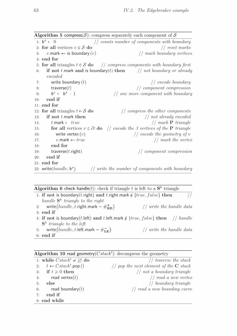
63 IV.2. The Edgebreaker example

Algorithm 5 compress(S): compress separately each component of S1: b� Ð 0 // counts number of components with boundary2: for all vertices v P S do // reset marks3: v.mark Ð is boundary pvq // mark boundary vertices4: end for5: for all triangles t P S do // compress components with boundary first6: if not t.mark and is boundaryptq then // not boundary or already

encoded7: write boundary ptq // encode boundary8: traverseptq // component compression9: b� Ð b� � 1 // one more component with boundary

10: end if11: end for12: for all triangles t P S do // compress the other components13: if not t.mark then // not already encoded14: t.mark Ð true // mark P triangle15: for all vertices v P Bt do // encode the 3 vertices of the P triangle16: write vertex pvq // encode the geometry of v17: v.mark Ð true // mark the vertex18: end for19: traversept.rightq // component compression20: end if21: end for22: writephandle, b�q // write the number of components with boundary

Algorithm 6 check handle(t): check if triangle t is left to a Sh triangle

1: if not is boundarypt.rightq and t.right.mark R ttrue, falseu then //handle Sh triangle to the right

2: write�handle, t.right.mark�#�

RE

�// write the handle data

3: end if4: if not is boundarypt.leftq and t.left.mark R ttrue, falseu then // handle

Sh triangle to the left5: write

�handle, t.left.mark�#�

LE

�// write the handle data

6: end if

Algorithm 10 read geometry(Cstack1): decompress the geometry

1: while Cstack1 � H do // traverse the stack2: t Ð Cstack1.pop pq // pop the next element of the C stack3: if t ¥ 0 then // not a boundary triangle4: read vertexptq // read a new vertex5: else // boundary triangle6: read boundaryptq // read a new bounding curve7: end if8: end while

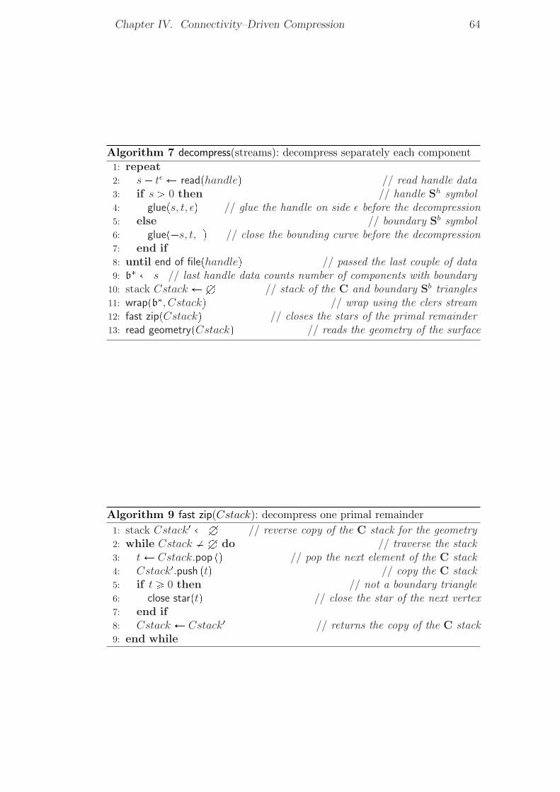
Chapter IV. Connectivity–Driven Compression 64

Algorithm 7 decompress(streams): decompress separately each component

1: repeat2: s� tε Ð readphandleq // read handle data3: if s ¡ 0 then // handle Sh symbol4: glueps, t, εq // glue the handle on side ε before the decompression5: else // boundary Sb symbol6: gluep�s, t,�q // close the bounding curve before the decompression7: end if8: until end of filephandleq // passed the last couple of data9: b� Ð s // last handle data counts number of components with boundary

10: stack Cstack ÐH // stack of the C and boundary Sb triangles11: wrappb�, Cstackq // wrap using the clers stream12: fast zippCstackq // closes the stars of the primal remainder13: read geometrypCstackq // reads the geometry of the surface

Algorithm 9 fast zip(Cstack): decompress one primal remainder

1: stack Cstack1 ÐH // reverse copy of the C stack for the geometry2: while Cstack � H do // traverse the stack3: t Ð Cstack.pop pq // pop the next element of the C stack4: Cstack1.push ptq // copy the C stack5: if t ¥ 0 then // not a boundary triangle6: close starptq // close the star of the next vertex7: end if8: Cstack Ð Cstack1 // returns the copy of the C stack9: end while

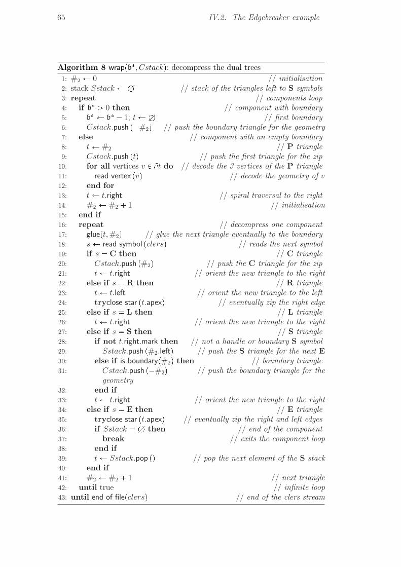
65 IV.2. The Edgebreaker example

Algorithm 8 wrappb�, Cstackq: decompress the dual trees

1: #2 Ð 0 // initialisation2: stack Sstack ÐH // stack of the triangles left to S symbols3: repeat // components loop4: if b� ¡ 0 then // component with boundary5: b� Ð b� � 1; t ÐH // first boundary6: Cstack.push p�#2q // push the boundary triangle for the geometry7: else // component with an empty boundary8: t Ð #2 // P triangle9: Cstack.push ptq // push the first triangle for the zip

10: for all vertices v P Bt do // decode the 3 vertices of the P triangle11: read vertex pvq // decode the geometry of v12: end for13: t Ð t.right // spiral traversal to the right14: #2 Ð #2 � 1 // initialisation15: end if16: repeat // decompress one component17: gluept, #2q // glue the next triangle eventually to the boundary18: s Ð read symbol pclersq // reads the next symbol19: if s � C then // C triangle20: Cstack.push p#2q // push the C triangle for the zip21: t Ð t.right // orient the new triangle to the right22: else if s � R then // R triangle23: t Ð t.left // orient the new triangle to the left24: tryclose star pt.apexq // eventually zip the right edge25: else if s � L then // L triangle26: t Ð t.right // orient the new triangle to the right27: else if s � S then // S triangle28: if not t.right.mark then // not a handle or boundary S symbol29: Sstack.push p#2.leftq // push the S triangle for the next E30: else if is boundaryp#2q then // boundary triangle31: Cstack.push p�#2q // push the boundary triangle for the

geometry32: end if33: t Ð t.right // orient the new triangle to the right34: else if s � E then // E triangle35: tryclose star pt.apexq // eventually zip the right and left edges36: if Sstack � H then // end of the component37: break // exits the component loop38: end if39: t Ð Sstack.pop pq // pop the next element of the S stack40: end if41: #2 Ð #2 � 1 // next triangle42: until true // infinite loop43: until end of filepclersq // end of the clers stream

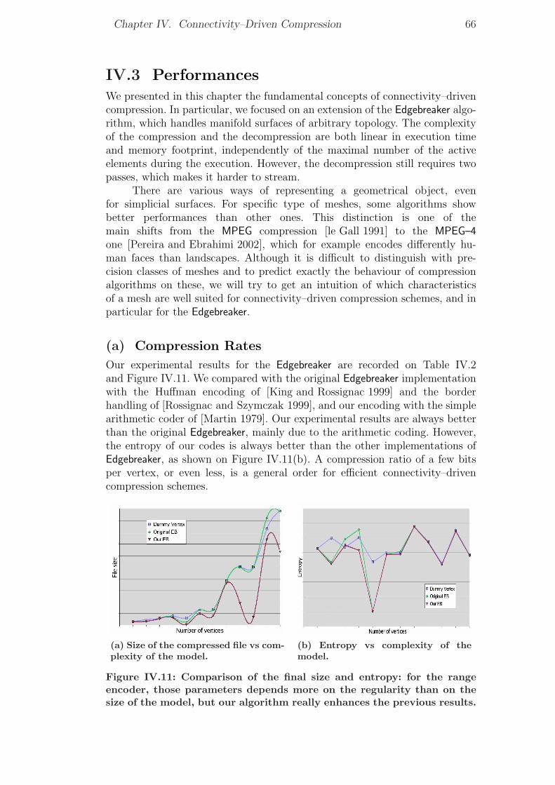
Chapter IV. Connectivity–Driven Compression 66

IV.3 PerformancesWe presented in this chapter the fundamental concepts of connectivity–drivencompression. In particular, we focused on an extension of the Edgebreaker algo-rithm, which handles manifold surfaces of arbitrary topology. The complexityof the compression and the decompression are both linear in execution timeand memory footprint, independently of the maximal number of the activeelements during the execution. However, the decompression still requires twopasses, which makes it harder to stream.

There are various ways of representing a geometrical object, evenfor simplicial surfaces. For specific type of meshes, some algorithms showbetter performances than other ones. This distinction is one of themain shifts from the MPEG compression [le Gall 1991] to the MPEG–4one [Pereira and Ebrahimi 2002], which for example encodes differently hu-man faces than landscapes. Although it is difficult to distinguish with pre-cision classes of meshes and to predict exactly the behaviour of compressionalgorithms on these, we will try to get an intuition of which characteristicsof a mesh are well suited for connectivity–driven compression schemes, and inparticular for the Edgebreaker.

(a) Compression Rates

Our experimental results for the Edgebreaker are recorded on Table IV.2and Figure IV.11. We compared with the original Edgebreaker implementationwith the Huffman encoding of [King and Rossignac 1999] and the borderhandling of [Rossignac and Szymczak 1999], and our encoding with the simplearithmetic coder of [Martin 1979]. Our experimental results are always betterthan the original Edgebreaker, mainly due to the arithmetic coding. However,the entropy of our codes is always better than the other implementations ofEdgebreaker, as shown on Figure IV.11(b). A compression ratio of a few bitsper vertex, or even less, is a general order for efficient connectivity–drivencompression schemes.

(a) Size of the compressed file vs com-plexity of the model.

(b) Entropy vs complexity of themodel.

Figure IV.11: Comparison of the final size and entropy: for the rangeencoder, those parameters depends more on the regularity than on thesize of the model, but our algorithm really enhances the previous results.

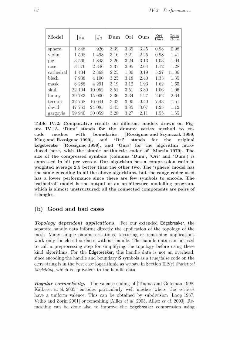
67 IV.3. Performances

Model |#0| |#2| Dum Ori Ours OriOurs

DumOurs

sphere 1 848 926 3.39 3.39 3.45 0.98 0.98violin 1 508 1 498 3.16 2.21 2.25 0.98 1.41pig 3 560 1 843 3.26 3.24 3.13 1.03 1.04rose 3 576 2 346 3.37 2.95 2.64 1.12 1.28cathedral 1 434 2 868 2.25 1.00 0.19 5.27 11.86blech 7 938 4 100 3.25 3.18 2.40 1.33 1.35mask 8 288 4 291 3.19 3.12 1.93 1.62 1.65skull 22 104 10 952 3.51 3.51 3.30 1.06 1.06bunny 29 783 15 000 3.36 3.34 1.27 2.62 2.64terrain 32 768 16 641 3.03 3.00 0.40 7.43 7.51david 47 753 24 085 3.45 3.85 3.07 1.25 1.12gargoyle 59 940 30 059 3.28 3.27 2.11 1.55 1.55

Table IV.2: Comparative results on different models drawn on Fig-ure IV.13. ‘Dum’ stands for the dummy vertex method to en-code meshes with boundaries [Rossignac and Szymczak 1999,King and Rossignac 1999], and ‘Ori’ stands for the originalEdgebreaker [Rossignac 1999], and ‘Ours’ for the algorithm intro-duced here, with the simple arithmetic coder of [Martin 1979]. Thesize of the compressed symbols (columns ‘Dum’, ‘Ori’ and ‘Ours’) isexpressed in bit per vertex. Our algorithm has a compression ratio inweighted average 2.5 better than the other two. The ‘sphere’ model hasthe same encoding in all the above algorithms, but the range coder usedhas a lower performance since there are few symbols to encode. The‘cathedral’ model is the output of an architecture modelling program,which is almost unstructured: all the connected components are pairs oftriangles.

(b) Good and bad cases

Topology–dependent applications. For our extended Edgebreaker, theseparate handle data informs directly the application of the topology of themesh. Many simple parameterisations, texturing or remeshing applicationswork only for closed surfaces without handle. The handle data can be usedto call a preprocessing step for simplifying the topology before using thesekind algorithms. For the Edgebreaker, this handle data is not an overhead,since encoding the handle and boundary S symbols as a true/false code on theclers string is in the best case logarithmic as we saw in Section II.2(c) StatisticalModelling, which is equivalent to the handle data.

Regular connectivity. The valence coding of [Touma and Gotsman 1998,Kalberer et al. 2005] encodes particularly well meshes where the verticeshave a uniform valence. This can be obtained by subdivision [Loop 1987,Velho and Zorin 2001] or remeshing [Alliez et al. 2003, Alliez et al. 2003]. Re-meshing can be done also to improve the Edgebreaker compression using

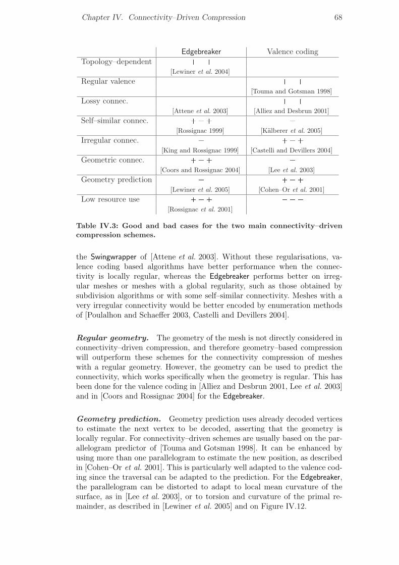
Chapter IV. Connectivity–Driven Compression 68

Edgebreaker Valence codingTopology–dependent ��� ���

[Lewiner et al. 2004]Regular valence ��� ���

[Touma and Gotsman 1998]Lossy connec. � ���

[Attene et al. 2003] [Alliez and Desbrun 2001]Self–similar connec. ��� �

[Rossignac 1999] [Kalberer et al. 2005]Irregular connec. � ���

[King and Rossignac 1999] [Castelli and Devillers 2004]Geometric connec. ��� �

[Coors and Rossignac 2004] [Lee et al. 2003]Geometry prediction � ���

[Lewiner et al. 2005] [Cohen–Or et al. 2001]Low resource use ��� ���

[Rossignac et al. 2001]

Table IV.3: Good and bad cases for the two main connectivity–drivencompression schemes.

the Swingwrapper of [Attene et al. 2003]. Without these regularisations, va-lence coding based algorithms have better performance when the connec-tivity is locally regular, whereas the Edgebreaker performs better on irreg-ular meshes or meshes with a global regularity, such as those obtained bysubdivision algorithms or with some self–similar connectivity. Meshes with avery irregular connectivity would be better encoded by enumeration methodsof [Poulalhon and Schaeffer 2003, Castelli and Devillers 2004].

Regular geometry. The geometry of the mesh is not directly considered inconnectivity–driven compression, and therefore geometry–based compressionwill outperform these schemes for the connectivity compression of mesheswith a regular geometry. However, the geometry can be used to predict theconnectivity, which works specifically when the geometry is regular. This hasbeen done for the valence coding in [Alliez and Desbrun 2001, Lee et al. 2003]and in [Coors and Rossignac 2004] for the Edgebreaker.

Geometry prediction. Geometry prediction uses already decoded verticesto estimate the next vertex to be decoded, asserting that the geometry islocally regular. For connectivity–driven schemes are usually based on the par-allelogram predictor of [Touma and Gotsman 1998]. It can be enhanced byusing more than one parallelogram to estimate the new position, as describedin [Cohen–Or et al. 2001]. This is particularly well adapted to the valence cod-ing since the traversal can be adapted to the prediction. For the Edgebreaker,the parallelogram can be distorted to adapt to local mean curvature of thesurface, as in [Lee et al. 2003], or to torsion and curvature of the primal re-mainder, as described in [Lewiner et al. 2005] and on Figure IV.12.

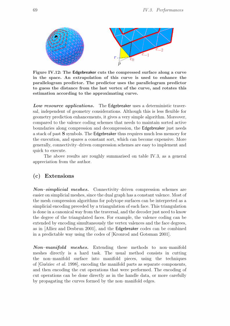
69 IV.3. Performances

Figure IV.12: The Edgebreaker cuts the compressed surface along a curvein the space. An extrapolation of this curve is used to enhance theparallelogram predictor. The predictor uses the parallelogram predictorto guess the distance from the last vertex of the curve, and rotates thisestimation according to the approximating curve.

Low resource applications. The Edgebreaker uses a deterministic traver-sal, independent of geometry considerations. Although this is less flexible forgeometry prediction enhancements, it gives a very simple algorithm. Moreover,compared to the valence coding schemes that needs to maintain sorted activeboundaries along compression and decompression, the Edgebreaker just needsa stack of past S symbols. The Edgebreaker thus requires much less memory forthe execution, and spares a constant sort, which can become expensive. Moregenerally, connectivity–driven compression schemes are easy to implement andquick to execute.

The above results are roughly summarised on table IV.3, as a generalappreciation from the author.

(c) Extensions

Non–simplicial meshes. Connectivity–driven compression schemes areeasier on simplicial meshes, since the dual graph has a constant valence. Most ofthe mesh compression algorithms for polytope surfaces can be interpreted as asimplicial encoding preceded by a triangulation of each face. This triangulationis done in a canonical way from the traversal, and the decoder just need to knowthe degree of the triangulated faces. For example, the valence coding can beextended by encoding simultaneously the vertex valences and the face degrees,as in [Alliez and Desbrun 2001], and the Edgebreaker codes can be combinedin a predictable way using the codes of [Kronrod and Gotsman 2001].

Non–manifold meshes. Extending these methods to non–manifoldmeshes directly is a hard task. The usual method consists in cuttingthe non–manifold surface into manifold pieces, using the techniquesof [Gueziec et al. 1998], encoding the manifold parts as separate components,and then encoding the cut operations that were performed. The encoding ofcut operations can be done directly as in the handle data, or more carefullyby propagating the curves formed by the non–manifold edges.

Chapter IV. Connectivity–Driven Compression 70

Higher dimensions. For solid meshes, the Edgebreaker compressionhas been directly extended to tetrahedral meshes in [Gumhold et al. 1999,Szymczak and Rossignac 2000], and the valence coding has been extendedin [Isenburg and Alliez 2002]. The principles are the same, but the encodingneeds some extra information to complete the intermediate dimension betweenthe spanning tree and the remainders. This extra information has necessarilysome expensive parts to encode, similar to the handle S symbols that are nec-essary to glue distant parts of the traversal. Minimising this extra informationis an NP–hard problem, as proved in [Lewiner et al. 2004]. For higher dimen-sions, the combinatory of mesh connectivity makes it difficult to find a conciseset of symbols for coding, or a good statistical model for them as was donefor surfaces in [King and Rossignac 1999]. However, for high codimensions, theconnectivity remains simple while the geometry can be efficiently predicted.Seen from the other side, this means that for low codimension, geometry–basedcoding can be very efficient, which is where isosurface compression outperformsany connectivity–based compression, as we will see in the next chapter.

Robustness. The Edgebreaker is robust in the sense that it handles generalmanifold surfaces. However, it is not particularly robust with a noisy transmis-sion, where the clers codes can be altered. In that case, the grammar inherentto these codes can be used to detect transmission errors, but not directly tocorrect them.

Deformable meshes. For animation purposes, the Edgebreaker can be useddirectly to compute the deformed mesh when its connectivity is constant,and using for example [Sorkine et al. 2003] to interpolate the geometry. Localchanges in the connectivity can be further encoded using the explicit identifi-cation of vertices and triangles provided by the Edgebreaker, similarly to thedescription of [Vieira et al. 2004].

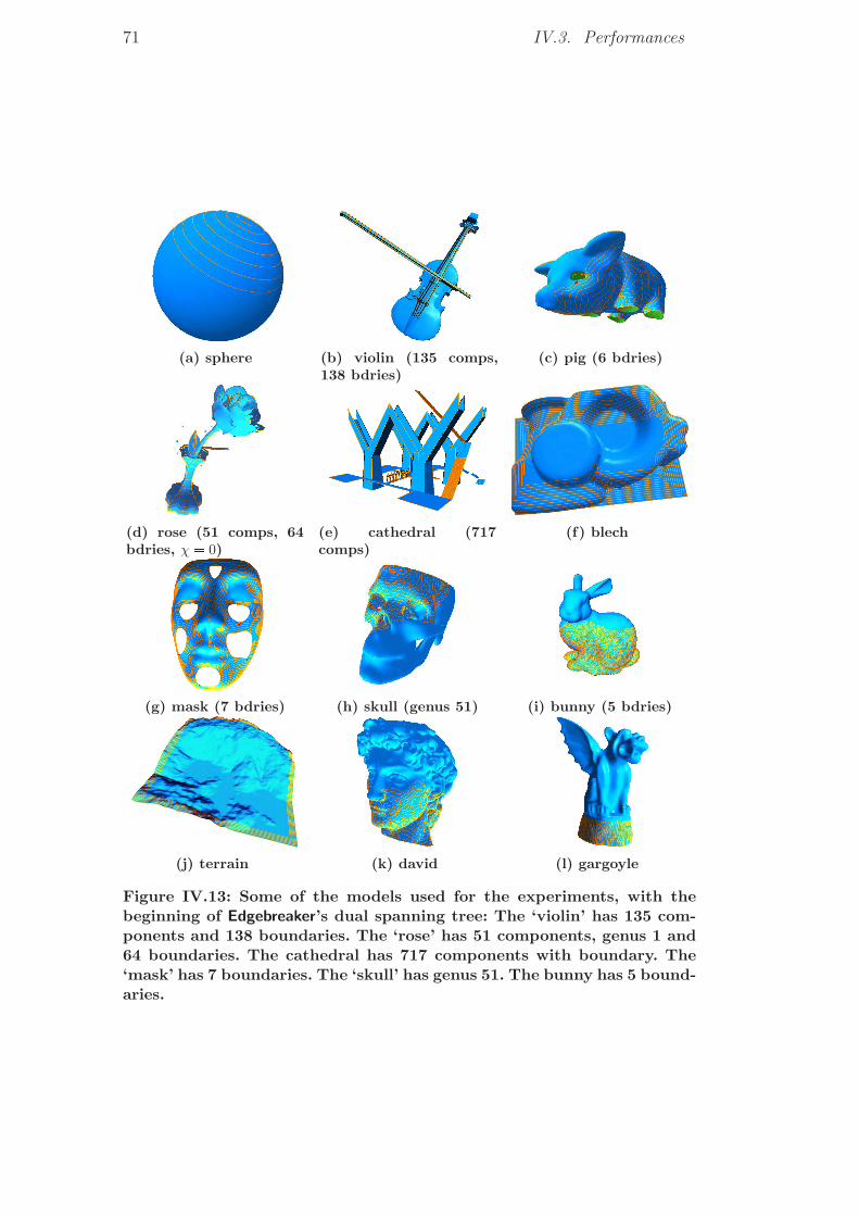
71 IV.3. Performances

(a) sphere (b) violin (135 comps,138 bdries)

(c) pig (6 bdries)

(d) rose (51 comps, 64bdries, χ � 0)

(e) cathedral (717comps)

(f) blech

(g) mask (7 bdries) (h) skull (genus 51) (i) bunny (5 bdries)

(j) terrain (k) david (l) gargoyle

Figure IV.13: Some of the models used for the experiments, with thebeginning of Edgebreaker’s dual spanning tree: The ‘violin’ has 135 com-ponents and 138 boundaries. The ‘rose’ has 51 components, genus 1 and64 boundaries. The cathedral has 717 components with boundary. The‘mask’ has 7 boundaries. The ‘skull’ has genus 51. The bunny has 5 bound-aries.

VLevel Set Compression

Connectivity–driven compression schemes provide general methods with goodperformances in average. However, for specific cases, their compression ratiosare far away from those of dedicated techniques. This chapter describesthe specific case of isosurface compression, and more generally level setscompression, where compression ratio can achieve fractions of connectivity–driven ones for the connectivity and the geometry (from 8–10 bits per vertex toonly 1 or 2). This mixture with geometry is the key to reach these performances.

Level sets. A level set is the preimage f�1 p0q of the singleton t0u bya continuous function f : X Ñ R. The domain X of f is generally anEuclidean space Rd. If f is continuously differentiable, this implies from Sard’stheorem [Arnold 1981] that the level set is generically a manifold of dimensiond� 1 with an empty boundary. In the discrete setting, the sampling f off will be called the scalar data, and the points x of X where f is definedwill be called the sample points . The discrete level set then depends on thesampling and on the interpolation. We chose one particular interpolation,detailed in Section V.1 Level Set Extraction.

(a) 764 bytes (b) 853 bytes (c) 1089 bytes (d) 2011 bytes (e) 5369 bytes

Figure V.1: Topology controlled extraction of a Computerized Tomogra-phy image of the cortex, and progressive compression.

Level curve compression. The first level sets to be encoded were con-tour curves (d � 2), especially for cartographic data and shape classifica-tion. When the scalar data is an image, and the sample points are limitedto the pixels of that image, the contour can be compressed using deriva-tives of the chain code of [Freeman 1974], or as a standard bidimensionalsignal as in [Langdon and Rissanen 1981, Bossen and Ebrahimi 1997]. Whenthe contour is more precise than pixel quantisation, the vector displace-ment inside that pixel can be compressed using [Craizer et al. 2002*1,

Chapter V. Level Set Compression 74

Safonova and Rossignac 2003]. These methods can be extended to hierarchi-cal representations, as in [Lopes et al. 2002*1], and then to progressive com-pression schemes, as done in [le Buhan and Ebrahimi 1997] by a hierarchicalrepresentation induced by a multiresolution of the image.

Isosurface applications. Isosurfaces (d � 3) are widely used inmany fields, from medical imaging [Lorensen and Cline 1987] to computergraphics [Parker et al. 1998] and surface reconstruction [Davis et al. 2002],through geophysical modelling [Tavares et al. 2003] and scientific visuali-sation [Bajaj et al. 1998]. For example, medical scan techniques such ascomputerised axial tomography and magnetic resonance imaging measurephysical quantities sampled on a semiregular tridimensional grid. Also forscientific simulations, partial differential equations are usually resolvedusing level set methods, as those of [Sethian 1999], which also result insampled functions over a tridimensional grid. This variety of applica-tions resulted also from a large panel of techniques to manipulate iso-surfaces [Bloomenthal et al. 1997]. These isosurfaces can be structured intomeshes by the usual Marching Cubes method of [Lorensen and Cline 1987]and its extensions [Nielson and Hamann 1991, Montani et al. 1994,Lewiner et al. 2003*3], the dual contouring of [Ju et al. 2002] and simpli-cial methods [Velho 1996, Treece et al. 1999].

Isosurface compression. In most of isosurface applications, the visualresult is only a surface extracted from the scalar data as an interpolationof f. For example, the cortex corresponds to only a specific X–ray scintillationinside the scan of the whole head. In that case, looking only at this cortex allowsdiscarding most of the scalar data, as the reconstructed cortex is contained onlyin a limited part of the head. This motivates specific techniques to compressisosurfaces by encoding only the essential portion of the scalar data. Moreover,these techniques show better performances than generic mesh compressionmethods. Although [Saupe and Kuska 2002] and [Yang and Wu 2002] alreadydeveloped specific compression schemes for isosurface, their extensive encodingbased on Marching Cubes’ configurations have been quickly bested by the JBIGcompression of the scalar data, and then by [Taubin 2002] who extended thisarithmetic encoding with a context in all three dimensions of scalar data.Then, [Boada and Navazo 2001] proposed to encode only the specific part ofthe scalar data containing the isosurface, in a progressive manner based onan octree decomposition of the scalar data. A small improvement of this workproposed in [Lee et al. 2003] to complete the compression with a final encodingof the geometry at the finest level of detail.

Simplicial level set compression. We will introduce now a generalmethod to compress level sets in any dimension, which is competitivewith the state–of–the–art for contour curves [le Buhan and Ebrahimi 1997]and isosurfaces [Lee et al. 2003]. This method was first introducedin [Lewiner et al. 2004*2, Lewiner et al. 2004*4, Lewiner et al. 2005*3], andcan be used for direct or progressive compression, as on Figure I.5. It is based

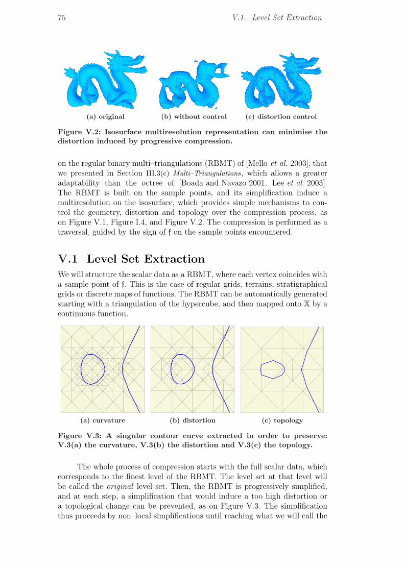
75 V.1. Level Set Extraction

(a) original (b) without control (c) distortion control

Figure V.2: Isosurface multiresolution representation can minimise thedistortion induced by progressive compression.

on the regular binary multi–triangulations (RBMT) of [Mello et al. 2003], thatwe presented in Section III.3(c) Multi–Triangulations, which allows a greateradaptability than the octree of [Boada and Navazo 2001, Lee et al. 2003].The RBMT is built on the sample points, and its simplification induce amultiresolution on the isosurface, which provides simple mechanisms to con-trol the geometry, distortion and topology over the compression process, ason Figure V.1, Figure I.4, and Figure V.2. The compression is performed as atraversal, guided by the sign of f on the sample points encountered.

V.1 Level Set ExtractionWe will structure the scalar data as a RBMT, where each vertex coincides witha sample point of f. This is the case of regular grids, terrains, stratigraphicalgrids or discrete maps of functions. The RBMT can be automatically generatedstarting with a triangulation of the hypercube, and then mapped onto X by acontinuous function.

(a) curvature (b) distortion (c) topology

Figure V.3: A singular contour curve extracted in order to preserve:V.3(a) the curvature, V.3(b) the distortion and V.3(c) the topology.

The whole process of compression starts with the full scalar data, whichcorresponds to the finest level of the RBMT. The level set at that level willbe called the original level set. Then, the RBMT is progressively simplified,and at each step, a simplification that would induce a too high distortion ora topological change can be prevented, as on Figure V.3. The simplificationthus proceeds by non–local simplifications until reaching what we will call the

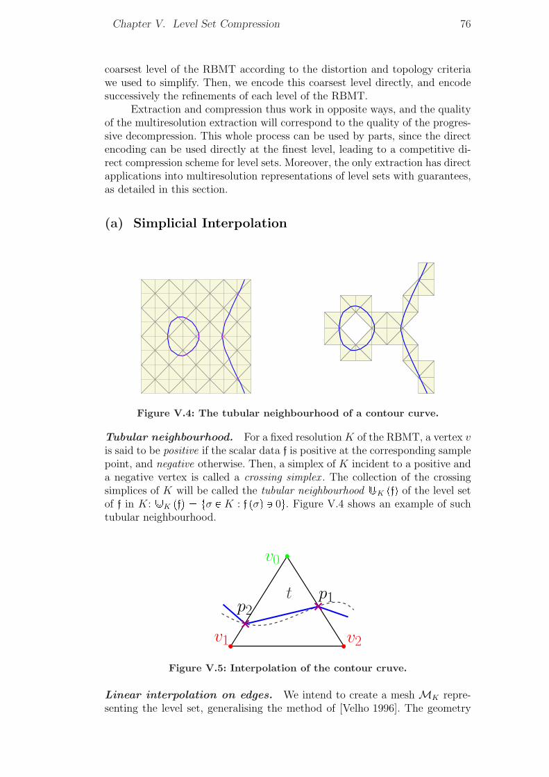
Chapter V. Level Set Compression 76

coarsest level of the RBMT according to the distortion and topology criteriawe used to simplify. Then, we encode this coarsest level directly, and encodesuccessively the refinements of each level of the RBMT.

Extraction and compression thus work in opposite ways, and the qualityof the multiresolution extraction will correspond to the quality of the progres-sive decompression. This whole process can be used by parts, since the directencoding can be used directly at the finest level, leading to a competitive di-rect compression scheme for level sets. Moreover, the only extraction has directapplications into multiresolution representations of level sets with guarantees,as detailed in this section.

(a) Simplicial Interpolation

Figure V.4: The tubular neighbourhood of a contour curve.

Tubular neighbourhood. For a fixed resolution K of the RBMT, a vertex vis said to be positive if the scalar data f is positive at the corresponding samplepoint, and negative otherwise. Then, a simplex of K incident to a positive anda negative vertex is called a crossing simplex . The collection of the crossingsimplices of K will be called the tubular neighbourhood ]K pfq of the level setof f in K: ]K pfq � tσ P K : f pσq Q 0u. Figure V.4 shows an example of suchtubular neighbourhood.

Figure V.5: Interpolation of the contour cruve.

Linear interpolation on edges. We intend to create a mesh MK repre-senting the level set, generalising the method of [Velho 1996]. The geometry

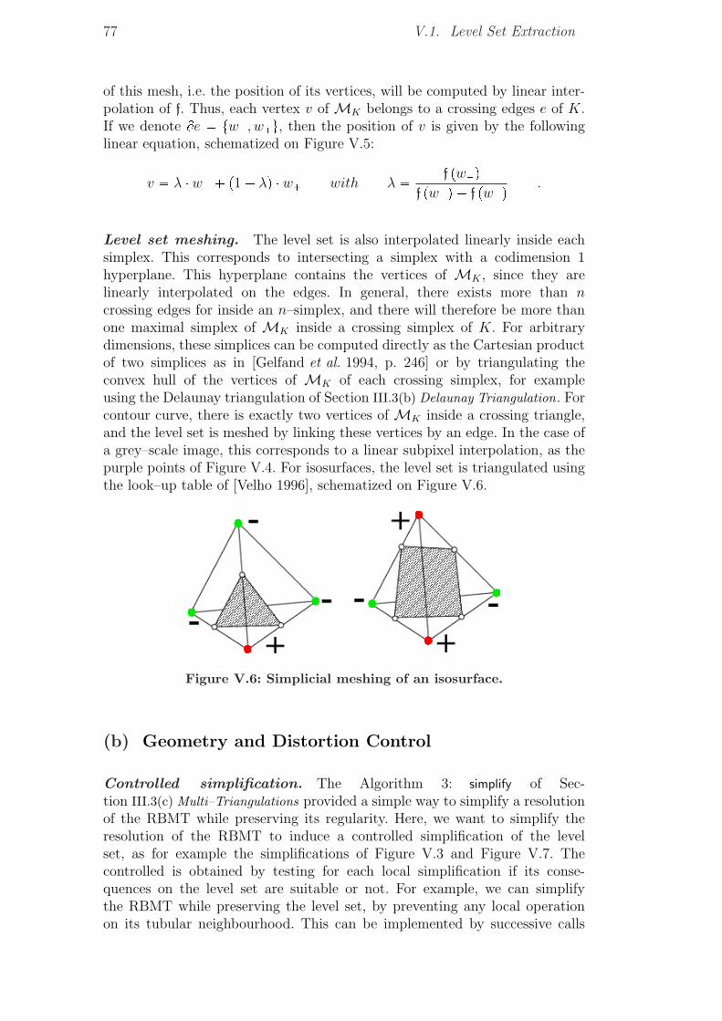
77 V.1. Level Set Extraction

of this mesh, i.e. the position of its vertices, will be computed by linear inter-polation of f. Thus, each vertex v of MK belongs to a crossing edges e of K.If we denote Be � tw�, w�u, then the position of v is given by the followinglinear equation, schematized on Figure V.5:

v � λ � w� � p1� λq � w� with λ � f pw�qf pw�q � f pw�q .

Level set meshing. The level set is also interpolated linearly inside eachsimplex. This corresponds to intersecting a simplex with a codimension 1hyperplane. This hyperplane contains the vertices of MK , since they arelinearly interpolated on the edges. In general, there exists more than ncrossing edges for inside an n–simplex, and there will therefore be more thanone maximal simplex of MK inside a crossing simplex of K. For arbitrarydimensions, these simplices can be computed directly as the Cartesian productof two simplices as in [Gelfand et al. 1994, p. 246] or by triangulating theconvex hull of the vertices of MK of each crossing simplex, for exampleusing the Delaunay triangulation of Section III.3(b) Delaunay Triangulation. Forcontour curve, there is exactly two vertices of MK inside a crossing triangle,and the level set is meshed by linking these vertices by an edge. In the case ofa grey–scale image, this corresponds to a linear subpixel interpolation, as thepurple points of Figure V.4. For isosurfaces, the level set is triangulated usingthe look–up table of [Velho 1996], schematized on Figure V.6.

Figure V.6: Simplicial meshing of an isosurface.

(b) Geometry and Distortion Control

Controlled simplification. The Algorithm 3: simplify of Sec-tion III.3(c) Multi–Triangulations provided a simple way to simplify a resolutionof the RBMT while preserving its regularity. Here, we want to simplify theresolution of the RBMT to induce a controlled simplification of the levelset, as for example the simplifications of Figure V.3 and Figure V.7. Thecontrolled is obtained by testing for each local simplification if its conse-quences on the level set are suitable or not. For example, we can simplifythe RBMT while preserving the level set, by preventing any local operationon its tubular neighbourhood. This can be implemented by successive calls

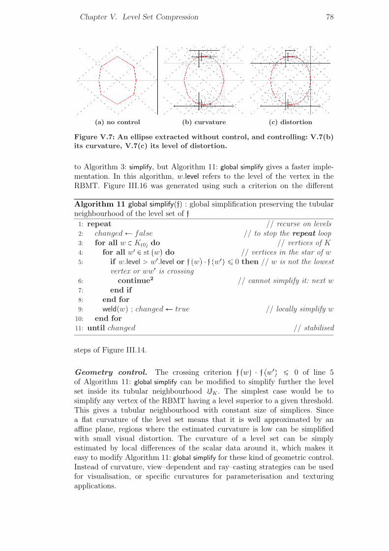
Chapter V. Level Set Compression 78

(a) no control (b) curvature (c) distortion

Figure V.7: An ellipse extracted without control, and controlling: V.7(b)its curvature, V.7(c) its level of distortion.

to Algorithm 3: simplify, but Algorithm 11: global simplify gives a faster imple-mentation. In this algorithm, w.level refers to the level of the vertex in theRBMT. Figure III.16 was generated using such a criterion on the different

Algorithm 11 global simplify(f) : global simplification preserving the tubularneighbourhood of the level set of f

1: repeat // recurse on levels2: changed Ð false // to stop the repeat loop3: for all w P Kp0q do // vertices of K4: for all w1 P st pwq do // vertices in the star of w5: if w.level ¡ w1.level or f pwq � f pw1q ¤ 0 then // w is not the lowest

vertex or ww1 is crossing6: continue2 // cannot simplify it: next w7: end if8: end for9: weld(w) ; changed Ð true // locally simplify w

10: end for11: until changed // stabilised

steps of Figure III.14.

Geometry control. The crossing criterion f pwq � f pw1q ¤ 0 of line 5of Algorithm 11: global simplify can be modified to simplify further the levelset inside its tubular neighbourhood ]K . The simplest case would be tosimplify any vertex of the RBMT having a level superior to a given threshold.This gives a tubular neighbourhood with constant size of simplices. Sincea flat curvature of the level set means that it is well approximated by anaffine plane, regions where the estimated curvature is low can be simplifiedwith small visual distortion. The curvature of a level set can be simplyestimated by local differences of the scalar data around it, which makes iteasy to modify Algorithm 11: global simplify for these kind of geometric control.Instead of curvature, view–dependent and ray–casting strategies can be usedfor visualisation, or specific curvatures for parameterisation and texturingapplications.

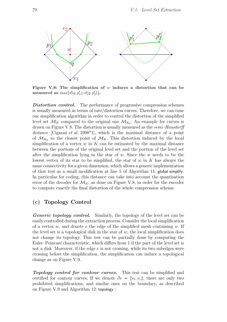
79 V.1. Level Set Extraction

Figure V.8: The simplification of w induces a distortion that can bemeasured as maxtdpq, p11q; dpq, p12qu.Distortion control. The performance of progressive compression schemesis usually measured in terms of rate/distortion curves. Therefore, we can tuneour simplification algorithm in order to control the distortion of the simplifiedlevel set MK compared to the original one MK0 . An example for curves isdrawn on Figure V.8. The distortion is usually measured as the semi–Hausdorffdistance [Cignoni et al. 1998*1], which is the maximal distance of a pointof MK0 to the closest point of MK . This distortion induced by the localsimplification of a vertex w in K can be estimated by the maximal distancebetween the portions of the original level set and the portion of the level setafter the simplification lying in the star of w. Since the w needs to be thelowest vertex of its star to be simplified, the star of w in K has always thesame connectivity for a given dimension, which allows a generic implementationof that test as a small modification at line 5 of Algorithm 11: global simplify.In particular for coding, this distance can take into account the quantisationerror of the decoder for MK , as done on Figure V.8, in order for the encoderto compute exactly the final distortion of the whole compression scheme.

(c) Topology Control

Generic topology control. Similarly, the topology of the level set can beeasily controlled during the extraction process. Consider the local simplificationof a vertex w, and denote e the edge of the simplified mesh containing w. Ifthe level set is a topological disk in the star of w, the local simplification doesnot change its topology. This test can be partially done by computing theEuler–Poincare characteristic, which differs from 1 if the part of the level set isnot a disk. Moreover, if the edge e is not crossing, while its two subedges werecrossing before the simplification, the simplification can induce a topologicalchange as on Figure V.9.

Topology control for contour curves. This test can be simplified andcertified for contour curves. If we denote Be � tvl, vru, there are only twoprohibited simplifications, and similar ones on the boundary, as describedon Figure V.9 and Algorithm 12: topology :

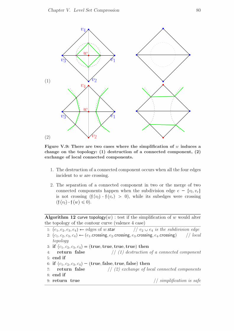
Chapter V. Level Set Compression 80

(1)

(2)

Figure V.9: There are two cases where the simplification of w induces achange on the topology: (1) destruction of a connected component, (2)exchange of local connected components.

1. The destruction of a connected component occurs when all the four edgesincident to w are crossing.

2. The separation of a connected component in two or the merge of twoconnected components happen when the subdivision edge e � tvl, vruis not crossing (f pvlq � f pvrq ¡ 0), while its subedges were crossing(f pvlq � f pwq ¤ 0).

Algorithm 12 curve topology(w) : test if the simplification of w would alterthe topology of the contour curve (valence 4 case)

1: pe1, e2, e3, e4q Ð edges of w.star // e2 Y e4 is the subdivision edge2: pc1, c2, c3, c4q Ð pe1.crossing, e2.crossing, e3.crossing, e4.crossingq // local

topology3: if pc1, c2, c3, c4q � ptrue, true, true, trueq then4: return false // (1) destruction of a connected component5: end if6: if pc1, c2, c3, c4q � ptrue, false, true, falseq then7: return false // (2) exchange of local connected components8: end if9: return true // simplification is safe

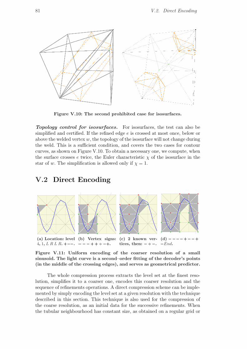
81 V.2. Direct Encoding

Figure V.10: The second prohibited case for isosurfaces.

Topology control for isosurfaces. For isosurfaces, the test can also besimplified and certified. If the refined edge e is crossed at most once, below orabove the welded vertex w, the topology of the isosurface will not change duringthe weld. This is a sufficient condition, and covers the two cases for contourcurves, as shown on Figure V.10. To obtain a necessary one, we compute, whenthe surface crosses e twice, the Euler characteristic χ of the isosurface in thestar of w. The simplification is allowed only if χ � 1.

V.2 Direct Encoding

(a) Location: level4, 1, L R L R. ���.

(b) Vertex signs:��������.(c) 2 known ver-tices, then: ���.

(d) ���������End.

Figure V.11: Uniform encoding of the coarser resolution of a smallsinusoid. The light curve is a second–order fitting of the decoder’s points(in the middle of the crossing edges), and serves as geometrical predictor.

The whole compression process extracts the level set at the finest reso-lution, simplifies it to a coarser one, encodes this coarser resolution and thesequence of refinements operations. A direct compression scheme can be imple-mented by simply encoding the level set at a given resolution with the techniquedescribed in this section. This technique is also used for the compression ofthe coarse resolution, as an initial data for the successive refinements. Whenthe tubular neighbourhood has constant size, as obtained on a regular grid or

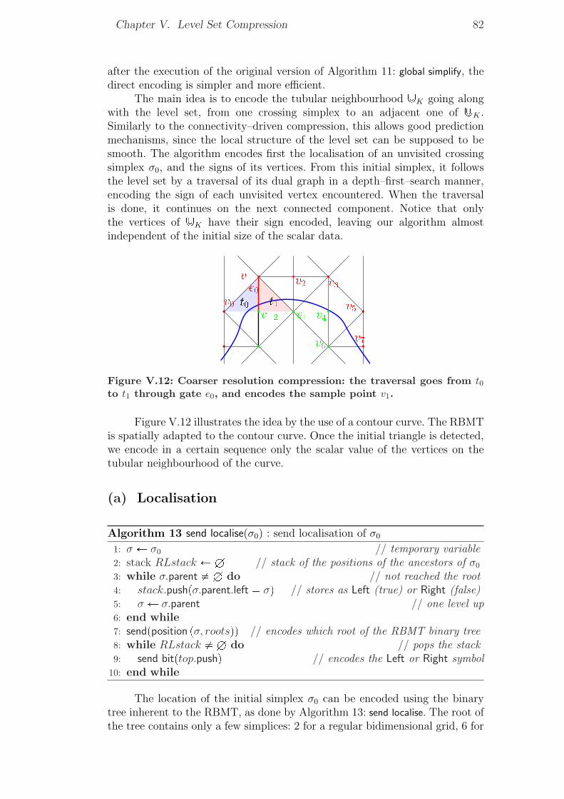
Chapter V. Level Set Compression 82

after the execution of the original version of Algorithm 11: global simplify, thedirect encoding is simpler and more efficient.

The main idea is to encode the tubular neighbourhood ]K going alongwith the level set, from one crossing simplex to an adjacent one of ]K .Similarly to the connectivity–driven compression, this allows good predictionmechanisms, since the local structure of the level set can be supposed to besmooth. The algorithm encodes first the localisation of an unvisited crossingsimplex σ0, and the signs of its vertices. From this initial simplex, it followsthe level set by a traversal of its dual graph in a depth–first–search manner,encoding the sign of each unvisited vertex encountered. When the traversalis done, it continues on the next connected component. Notice that onlythe vertices of ]K have their sign encoded, leaving our algorithm almostindependent of the initial size of the scalar data.

Figure V.12: Coarser resolution compression: the traversal goes from t0to t1 through gate e0, and encodes the sample point v1.

Figure V.12 illustrates the idea by the use of a contour curve. The RBMTis spatially adapted to the contour curve. Once the initial triangle is detected,we encode in a certain sequence only the scalar value of the vertices on thetubular neighbourhood of the curve.

(a) Localisation

Algorithm 13 send localise(σ0) : send localisation of σ0

1: σ Ð σ0 // temporary variable2: stack RLstack ÐH // stack of the positions of the ancestors of σ0

3: while σ.parent � H do // not reached the root4: stack.pushpσ.parent.left � σq // stores as Left (true) or Right (false)5: σ Ð σ.parent // one level up6: end while7: sendpposition pσ, rootsqq // encodes which root of the RBMT binary tree8: while RLstack � H do // pops the stack9: send bitptop.pushq // encodes the Left or Right symbol

10: end while

The location of the initial simplex σ0 can be encoded using the binarytree inherent to the RBMT, as done by Algorithm 13: send localise. The root ofthe tree contains only a few simplices: 2 for a regular bidimensional grid, 6 for

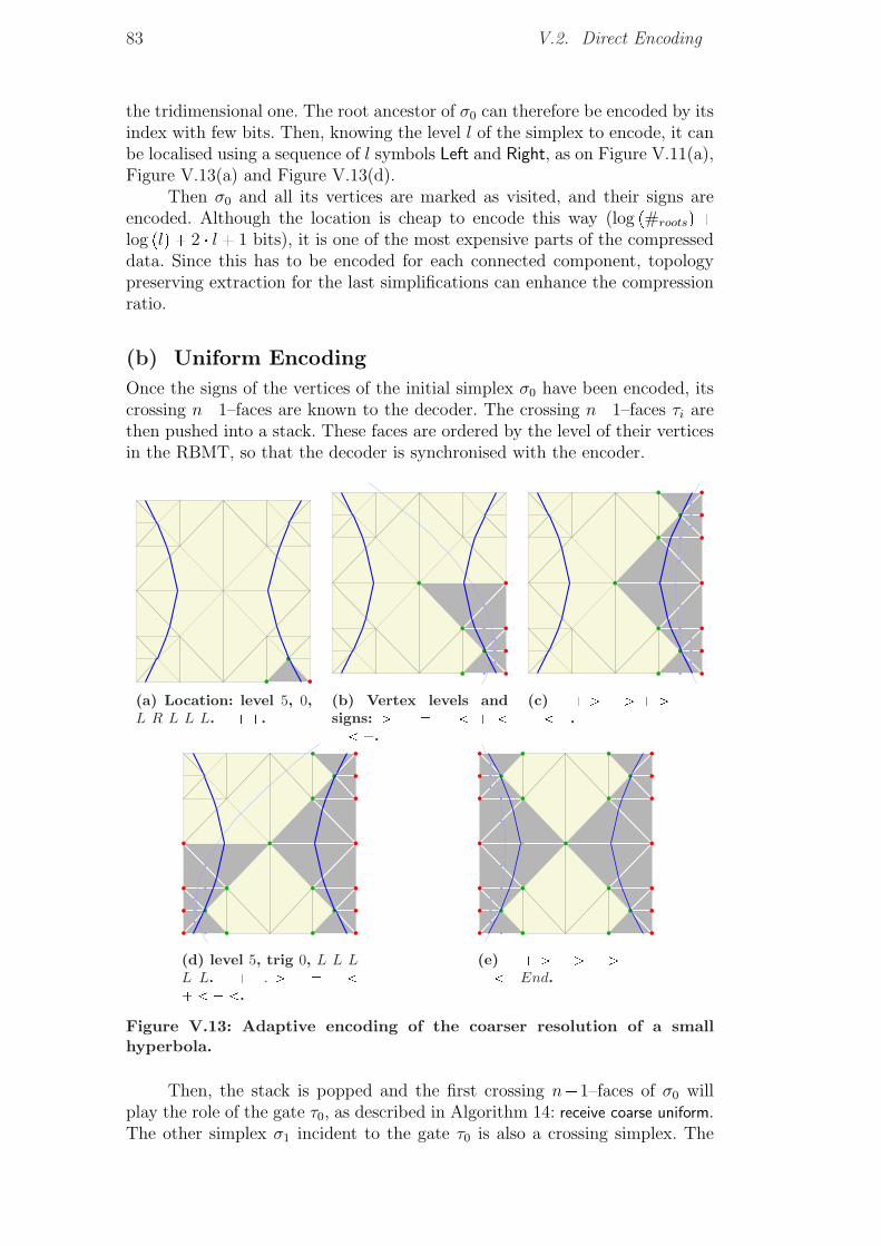
83 V.2. Direct Encoding

the tridimensional one. The root ancestor of σ0 can therefore be encoded by itsindex with few bits. Then, knowing the level l of the simplex to encode, it canbe localised using a sequence of l symbols Left and Right, as on Figure V.11(a),Figure V.13(a) and Figure V.13(d).

Then σ0 and all its vertices are marked as visited, and their signs areencoded. Although the location is cheap to encode this way (log p#rootsq �log plq � 2 � l � 1 bits), it is one of the most expensive parts of the compresseddata. Since this has to be encoded for each connected component, topologypreserving extraction for the last simplifications can enhance the compressionratio.

(b) Uniform Encoding

Once the signs of the vertices of the initial simplex σ0 have been encoded, itscrossing n�1–faces are known to the decoder. The crossing n�1–faces τi arethen pushed into a stack. These faces are ordered by the level of their verticesin the RBMT, so that the decoder is synchronised with the encoder.

(a) Location: level 5, 0,L R L L L. ���.

(b) Vertex levels andsigns: ¡ � � �   �  �   �.

(c) � � ¡ � ¡ � ¡ � ��   �.

(d) level 5, trig 0, L L LL L. � � �. ¡ � � �  �   �  .

(e) � � ¡ � ¡ � ¡ � ��   �End.

Figure V.13: Adaptive encoding of the coarser resolution of a smallhyperbola.

Then, the stack is popped and the first crossing n�1–faces of σ0 willplay the role of the gate τ0, as described in Algorithm 14: receive coarse uniform.The other simplex σ1 incident to the gate τ0 is also a crossing simplex. The

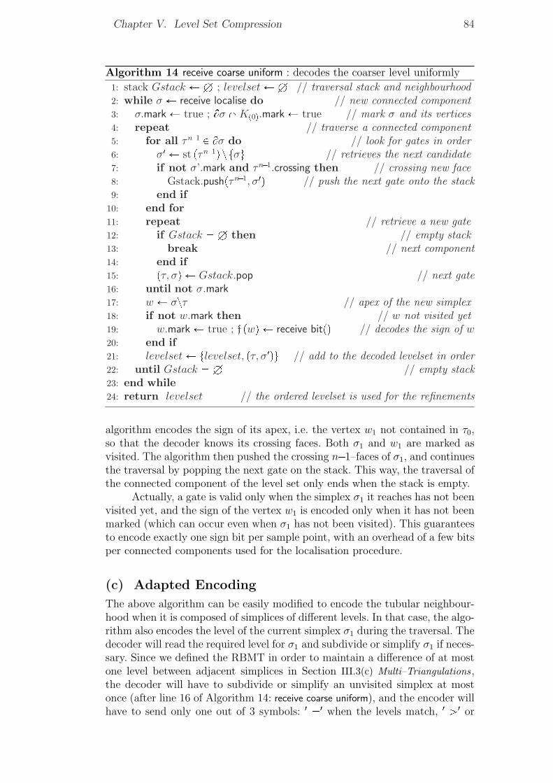
Chapter V. Level Set Compression 84

Algorithm 14 receive coarse uniform : decodes the coarser level uniformly

1: stack Gstack ÐH ; levelset ÐH // traversal stack and neighbourhood2: while σ Ð receive localise do // new connected component3: σ.mark Ð true ; Bσ XKp0q.mark Ð true // mark σ and its vertices4: repeat // traverse a connected component5: for all τn�1 P Bσ do // look for gates in order6: σ1 Ð st pτn�1q z tσu // retrieves the next candidate7: if not σ’.mark and τn�1.crossing then // crossing new face8: Gstack.pushpτn�1, σ1q // push the next gate onto the stack9: end if

10: end for11: repeat // retrieve a new gate12: if Gstack � H then // empty stack13: break // next component14: end if15: pτ, σq Ð Gstack.pop // next gate16: until not σ.mark17: w Ð σzτ // apex of the new simplex18: if not w.mark then // w not visited yet19: w.mark Ð true ; f pwq Ð receive bitpq // decodes the sign of w20: end if21: levelset Ð tlevelset, pτ, σ1qu // add to the decoded levelset in order22: until Gstack � H // empty stack23: end while24: return levelset // the ordered levelset is used for the refinements

algorithm encodes the sign of its apex, i.e. the vertex w1 not contained in τ0,so that the decoder knows its crossing faces. Both σ1 and w1 are marked asvisited. The algorithm then pushed the crossing n�1–faces of σ1, and continuesthe traversal by popping the next gate on the stack. This way, the traversal ofthe connected component of the level set only ends when the stack is empty.

Actually, a gate is valid only when the simplex σ1 it reaches has not beenvisited yet, and the sign of the vertex w1 is encoded only when it has not beenmarked (which can occur even when σ1 has not been visited). This guaranteesto encode exactly one sign bit per sample point, with an overhead of a few bitsper connected components used for the localisation procedure.

(c) Adapted Encoding

The above algorithm can be easily modified to encode the tubular neighbour-hood when it is composed of simplices of different levels. In that case, the algo-rithm also encodes the level of the current simplex σ1 during the traversal. Thedecoder will read the required level for σ1 and subdivide or simplify σ1 if neces-sary. Since we defined the RBMT in order to maintain a difference of at mostone level between adjacent simplices in Section III.3(c) Multi–Triangulations,the decoder will have to subdivide or simplify an unvisited simplex at mostonce (after line 16 of Algorithm 14: receive coarse uniform), and the encoder willhave to send only one out of 3 symbols: 1 �1 when the levels match, 1 ¡1 or

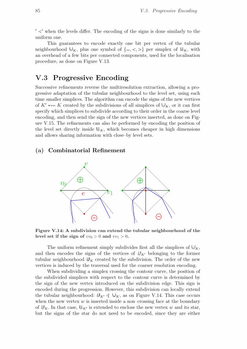
85 V.3. Progressive Encoding

1  1 when the levels differ. The encoding of the signs is done similarly to theuniform one.

This guarantees to encode exactly one bit per vertex of the tubularneighbourhood ]K , plus one symbol of t�, ,¡u per simplex of ]K , withan overhead of a few bits per connected components, used for the localisationprocedure, as done on Figure V.13.

V.3 Progressive EncodingSuccessive refinements reverse the multiresolution extraction, allowing a pro-gressive adaptation of the tubular neighbourhood to the level set, using eachtime smaller simplices. The algorithm can encode the signs of the new verticesof K 1 ø K created by the subdivisions of all simplices of ]K , or it can firstspecify which simplices to subdivide according to their order in the coarse levelencoding, and then send the sign of the new vertices inserted, as done on Fig-ure V.15. The refinements can also be performed by encoding the position ofthe level set directly inside ]K , which becomes cheaper in high dimensionsand allows sharing information with close–by level sets.

(a) Combinatorial Refinement

Figure V.14: A subdivision can extend the tubular neighbourhood of thelevel set if the sign of vv0 ¡ 0 and vv1 ¡ 0.

The uniform refinement simply subdivides first all the simplices of ]K ,and then encodes the signs of the vertices of ]K1 belonging to the formertubular neighbourhood ]K created by the subdivision. The order of the newvertices is induced by the traversal used for the coarser resolution encoding.

When subdividing a simplex crossing the contour curve, the position ofthe subdivided simplices with respect to the contour curve is determined bythe sign of the new vertex introduced on the subdivision edge. This sign isencoded during the progression. However, this subdivision can locally extendthe tubular neighbourhood: ]K1 � ]K , as on Figure V.14. This case occurswhen the new vertex w is inserted inside a non–crossing face at the boundaryof ]K . In that case, ]K1 is extended to enclose the new vertex w and its star,but the signs of the star do not need to be encoded, since they are either

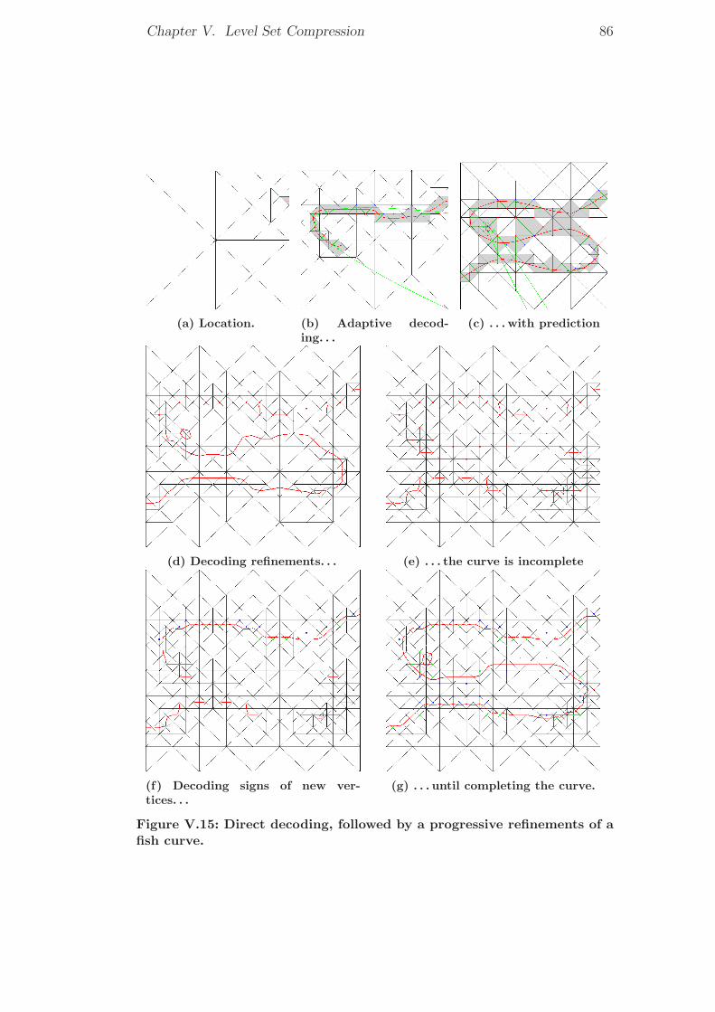
Chapter V. Level Set Compression 86

(a) Location. (b) Adaptive decod-ing. . .

(c) . . . with prediction

(d) Decoding refinements. . . (e) . . . the curve is incomplete

(f) Decoding signs of new ver-tices. . .

(g) . . . until completing the curve.

Figure V.15: Direct decoding, followed by a progressive refinements of afish curve.

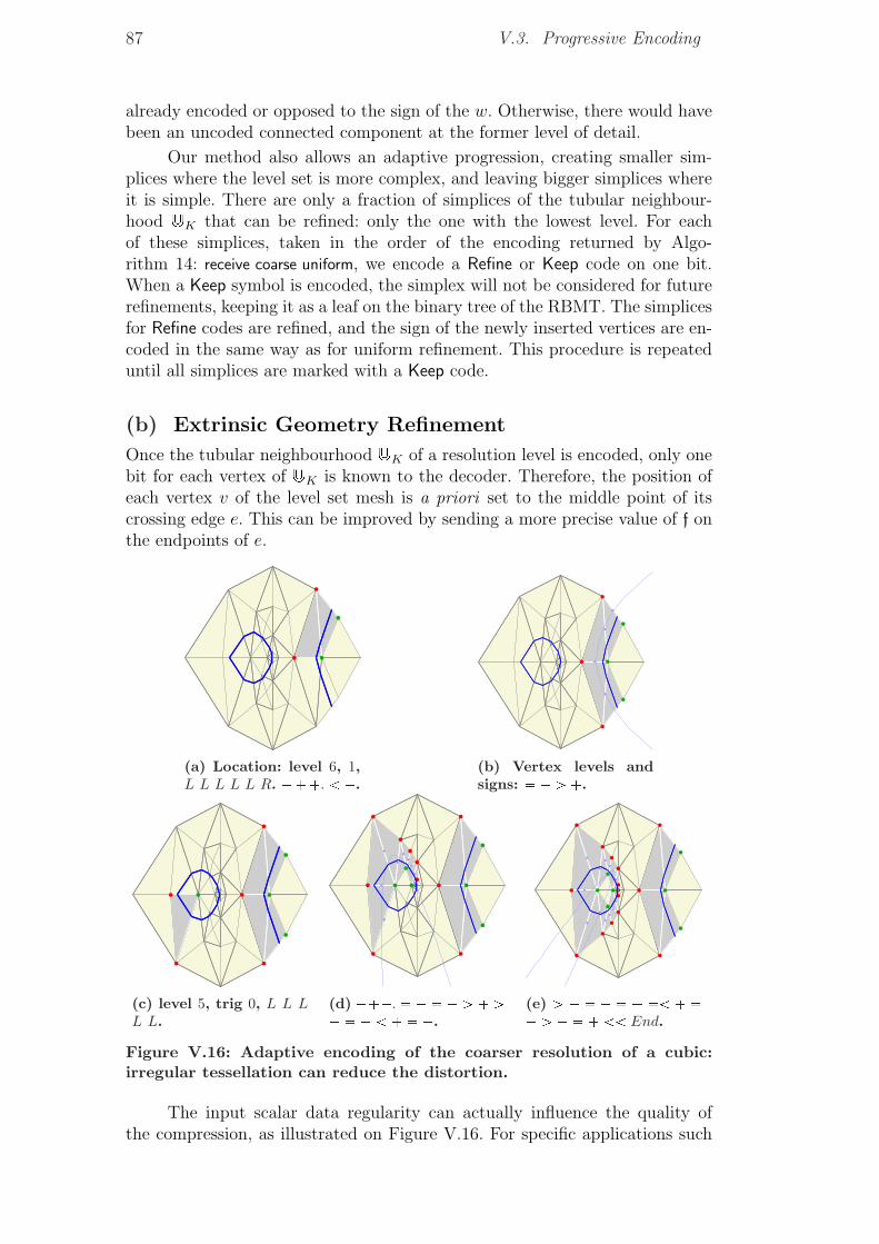
87 V.3. Progressive Encoding

already encoded or opposed to the sign of the w. Otherwise, there would havebeen an uncoded connected component at the former level of detail.

Our method also allows an adaptive progression, creating smaller sim-plices where the level set is more complex, and leaving bigger simplices whereit is simple. There are only a fraction of simplices of the tubular neighbour-hood ]K that can be refined: only the one with the lowest level. For eachof these simplices, taken in the order of the encoding returned by Algo-rithm 14: receive coarse uniform, we encode a Refine or Keep code on one bit.When a Keep symbol is encoded, the simplex will not be considered for futurerefinements, keeping it as a leaf on the binary tree of the RBMT. The simplicesfor Refine codes are refined, and the sign of the newly inserted vertices are en-coded in the same way as for uniform refinement. This procedure is repeateduntil all simplices are marked with a Keep code.

(b) Extrinsic Geometry Refinement

Once the tubular neighbourhood ]K of a resolution level is encoded, only onebit for each vertex of ]K is known to the decoder. Therefore, the position ofeach vertex v of the level set mesh is a priori set to the middle point of itscrossing edge e. This can be improved by sending a more precise value of f onthe endpoints of e.

(a) Location: level 6, 1,L L L L L R. ���.   �.

(b) Vertex levels andsigns: � � ¡ �.

(c) level 5, trig 0, L L LL L.

(d) ���. � � � � ¡ � ¡� � �   � � �.(e) ¡ � � � � � �  � �� ¡ � � �    End.

Figure V.16: Adaptive encoding of the coarser resolution of a cubic:irregular tessellation can reduce the distortion.

The input scalar data regularity can actually influence the quality ofthe compression, as illustrated on Figure V.16. For specific applications such

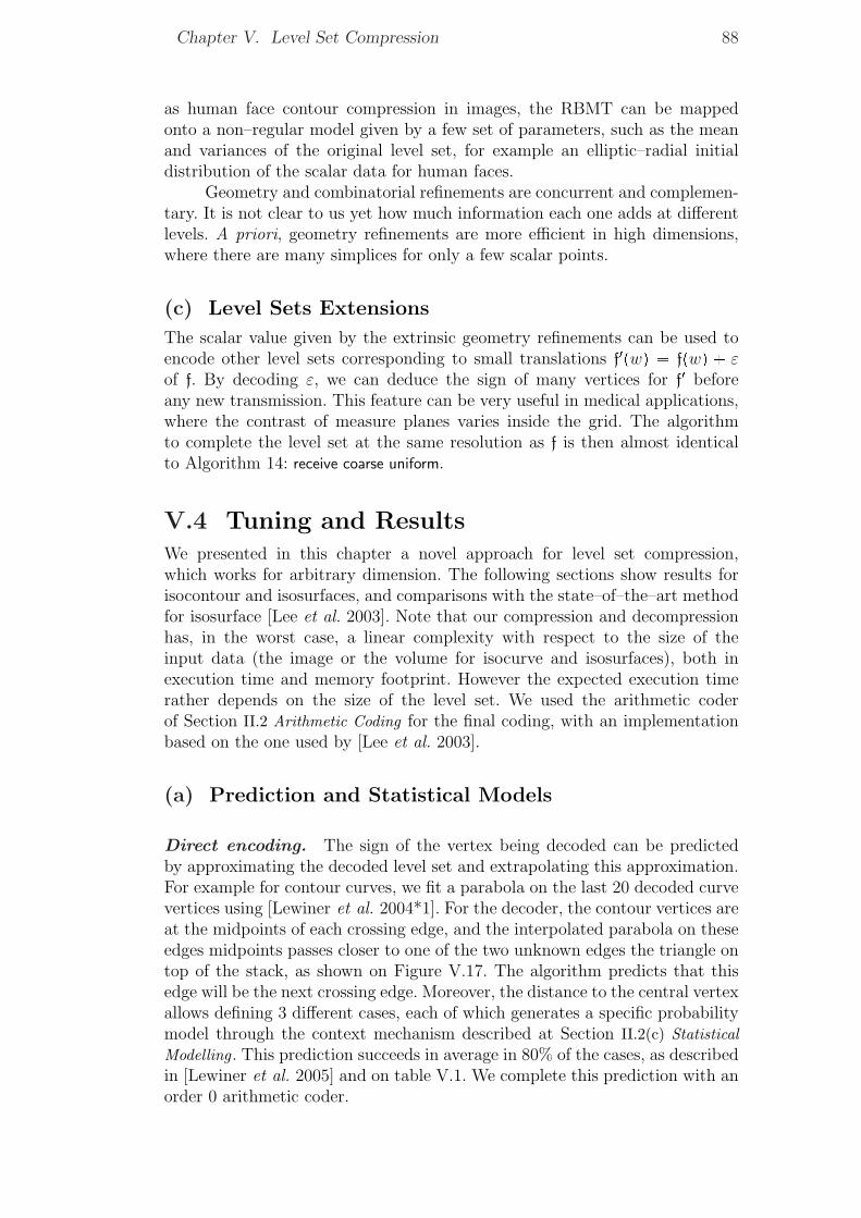
Chapter V. Level Set Compression 88

as human face contour compression in images, the RBMT can be mappedonto a non–regular model given by a few set of parameters, such as the meanand variances of the original level set, for example an elliptic–radial initialdistribution of the scalar data for human faces.

Geometry and combinatorial refinements are concurrent and complemen-tary. It is not clear to us yet how much information each one adds at differentlevels. A priori, geometry refinements are more efficient in high dimensions,where there are many simplices for only a few scalar points.

(c) Level Sets Extensions

The scalar value given by the extrinsic geometry refinements can be used toencode other level sets corresponding to small translations f1pwq � fpwq � εof f. By decoding ε, we can deduce the sign of many vertices for f1 beforeany new transmission. This feature can be very useful in medical applications,where the contrast of measure planes varies inside the grid. The algorithmto complete the level set at the same resolution as f is then almost identicalto Algorithm 14: receive coarse uniform.

V.4 Tuning and ResultsWe presented in this chapter a novel approach for level set compression,which works for arbitrary dimension. The following sections show results forisocontour and isosurfaces, and comparisons with the state–of–the–art methodfor isosurface [Lee et al. 2003]. Note that our compression and decompressionhas, in the worst case, a linear complexity with respect to the size of theinput data (the image or the volume for isocurve and isosurfaces), both inexecution time and memory footprint. However the expected execution timerather depends on the size of the level set. We used the arithmetic coderof Section II.2 Arithmetic Coding for the final coding, with an implementationbased on the one used by [Lee et al. 2003].

(a) Prediction and Statistical Models

Direct encoding. The sign of the vertex being decoded can be predictedby approximating the decoded level set and extrapolating this approximation.For example for contour curves, we fit a parabola on the last 20 decoded curvevertices using [Lewiner et al. 2004*1]. For the decoder, the contour vertices areat the midpoints of each crossing edge, and the interpolated parabola on theseedges midpoints passes closer to one of the two unknown edges the triangle ontop of the stack, as shown on Figure V.17. The algorithm predicts that thisedge will be the next crossing edge. Moreover, the distance to the central vertexallows defining 3 different cases, each of which generates a specific probabilitymodel through the context mechanism described at Section II.2(c) StatisticalModelling. This prediction succeeds in average in 80% of the cases, as describedin [Lewiner et al. 2005] and on table V.1. We complete this prediction with anorder 0 arithmetic coder.

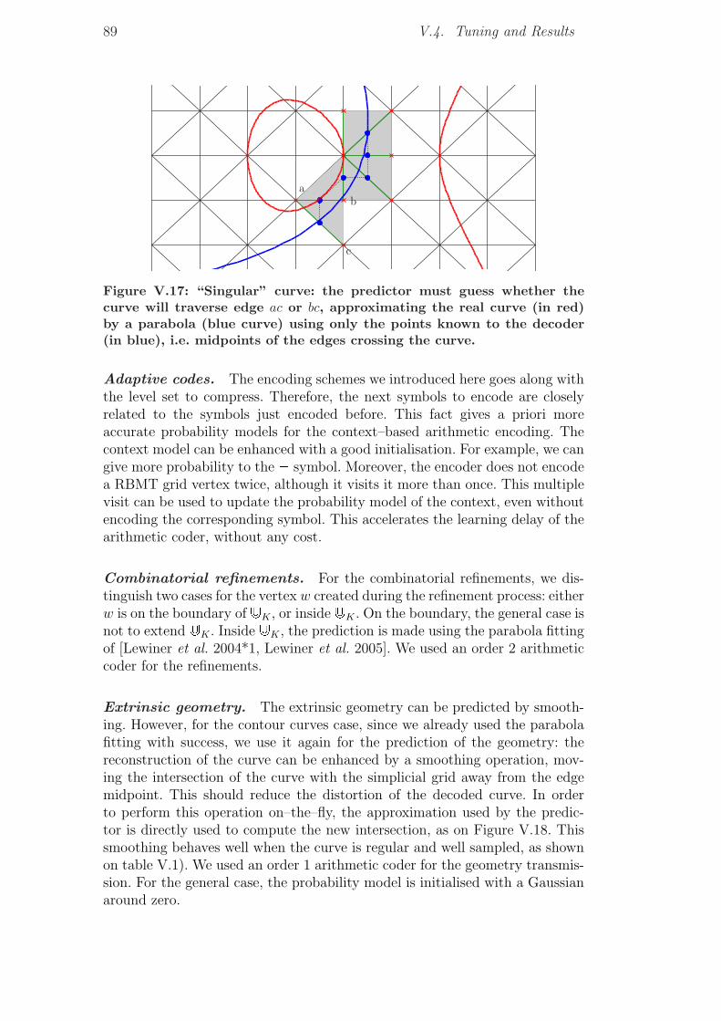
89 V.4. Tuning and Results

Figure V.17: “Singular” curve: the predictor must guess whether thecurve will traverse edge ac or bc, approximating the real curve (in red)by a parabola (blue curve) using only the points known to the decoder(in blue), i.e. midpoints of the edges crossing the curve.

Adaptive codes. The encoding schemes we introduced here goes along withthe level set to compress. Therefore, the next symbols to encode are closelyrelated to the symbols just encoded before. This fact gives a priori moreaccurate probability models for the context–based arithmetic encoding. Thecontext model can be enhanced with a good initialisation. For example, we cangive more probability to the � symbol. Moreover, the encoder does not encodea RBMT grid vertex twice, although it visits it more than once. This multiplevisit can be used to update the probability model of the context, even withoutencoding the corresponding symbol. This accelerates the learning delay of thearithmetic coder, without any cost.

Combinatorial refinements. For the combinatorial refinements, we dis-tinguish two cases for the vertex w created during the refinement process: eitherw is on the boundary of ]K , or inside ]K . On the boundary, the general case isnot to extend ]K . Inside ]K , the prediction is made using the parabola fittingof [Lewiner et al. 2004*1, Lewiner et al. 2005]. We used an order 2 arithmeticcoder for the refinements.

Extrinsic geometry. The extrinsic geometry can be predicted by smooth-ing. However, for the contour curves case, since we already used the parabolafitting with success, we use it again for the prediction of the geometry: thereconstruction of the curve can be enhanced by a smoothing operation, mov-ing the intersection of the curve with the simplicial grid away from the edgemidpoint. This should reduce the distortion of the decoded curve. In orderto perform this operation on–the–fly, the approximation used by the predic-tor is directly used to compute the new intersection, as on Figure V.18. Thissmoothing behaves well when the curve is regular and well sampled, as shownon table V.1). We used an order 1 arithmetic coder for the geometry transmis-sion. For the general case, the probability model is initialised with a Gaussianaround zero.

Chapter V. Level Set Compression 90

Figure V.18: A decompressed implicit sinoide without smoothing (left)and with the predictor on–the–fly smoothing (right).

Predict Size (bits) Distortion (10�3)Curve success w/out with gain w/out with gainbicorn 80.3 % 1479 1014 46 % 2.26 2.52 �10 %circle 80.6 % 1658 1106 50 % 2.38 2.20 8 %cubic 81.4 % 566 324 75 % 3.48 3.99 �13 %ellipse 82.5 % 1430 920 55 % 2.03 1.99 2 %singular 77.9 % 1501 1099 37 % 1.43 1.36 5 %hyperbola 80.2 % 1648 1164 42 % 1.53 1.39 10 %sinoide 84.5 % 2645 1612 64 % 0.91 0.76 20 %

Table V.1: Results of the predictor for the contour curves case: for eachone of the implicit curves, the number of successes over the erroneousguesses of the predictor is around 80%. The gain in the size of thecompressed curve is half of the compressed size. The smoothing inducedby the predictor reduces the distortion for most of the case. All the resultswere obtained as means of the same model over various resolution of thegrid, from 50 to 3000 vertices, with q � 84.

(b) Direct

The methods we introduced here are flexible and can be used in many ways,and resulted in nice rate/distortion curves, as on Figure V.22. For contourcurves in images, we started from the complete triangulation of the pixels. Forimplicit curves, we sent in–between two levels of detail a part of the geometry(2 bits). For any dimensions, single rate encoding is, as usual, a little moreefficient than progressive encoding.

(c) Progressive

The different controls on the adaptation of the multiresolution, such as thoseof Figure V.19, can have a significant cost, as shown on Figure V.22(a). Forexample, on regular models such as the elevation curve of the Sugar Loaf drawnon Figure V.20, the distortion and topology controls provide nicer results tothe eyes at the beginning of the compression than uniform refinements, while

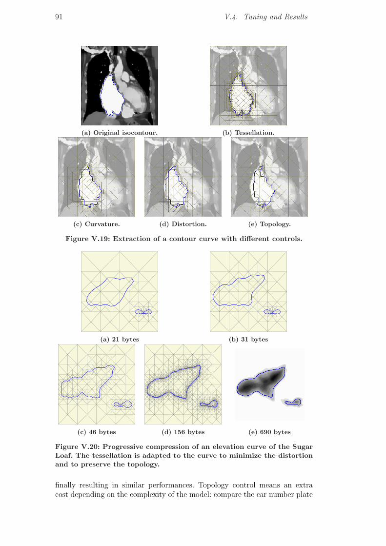
91 V.4. Tuning and Results

(a) Original isocontour. (b) Tessellation.

(c) Curvature. (d) Distortion. (e) Topology.

Figure V.19: Extraction of a contour curve with different controls.

(a) 21 bytes (b) 31 bytes

(c) 46 bytes (d) 156 bytes (e) 690 bytes

Figure V.20: Progressive compression of an elevation curve of the SugarLoaf. The tessellation is adapted to the curve to minimize the distortionand to preserve the topology.

finally resulting in similar performances. Topology control means an extracost depending on the complexity of the model: compare the car number plate

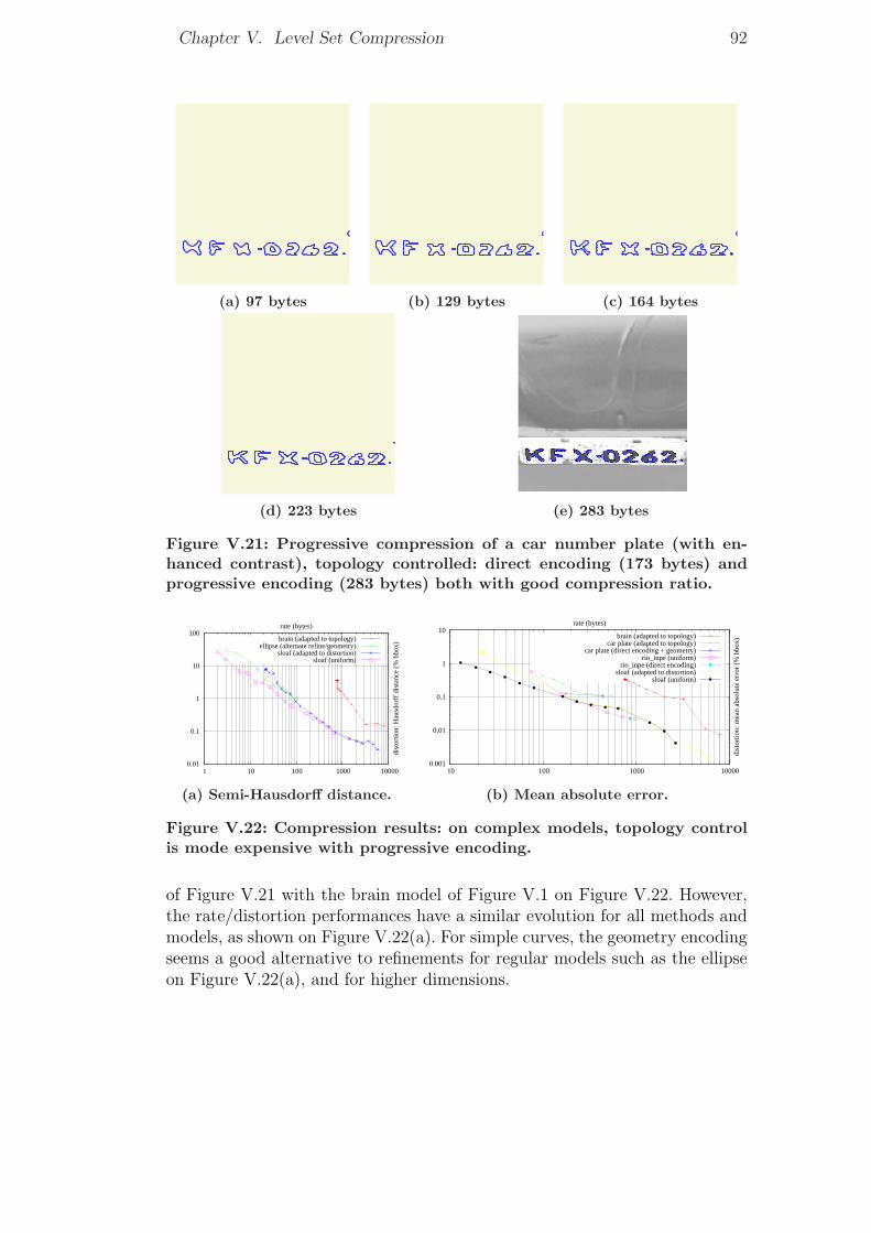
Chapter V. Level Set Compression 92

(a) 97 bytes (b) 129 bytes (c) 164 bytes

(d) 223 bytes (e) 283 bytes

Figure V.21: Progressive compression of a car number plate (with en-hanced contrast), topology controlled: direct encoding (173 bytes) andprogressive encoding (283 bytes) both with good compression ratio.

0.01

0.1

1

10

100

1 10 100 1000 10000

dist

ortio

n: H

ausd

orff

dis

tanc

e (%

bbo

x)

rate (bytes)

brain (adapted to topology)ellipse (alternate refine/geometry)

sloaf (adapted to distortion)sloaf (uniform)

(a) Semi-Hausdorff distance.

0.001

0.01

0.1

1

10

10 100 1000 10000

dist

ortio

n: m

ean

abso

lute

err

or (

% b

box)

rate (bytes)

brain (adapted to topology)car plate (adapted to topology)

car plate (direct encoding + geometry)rio_inpe (uniform)

rio_inpe (direct encoding)sloaf (adapted to distortion)

sloaf (uniform)

(b) Mean absolute error.

Figure V.22: Compression results: on complex models, topology controlis mode expensive with progressive encoding.

of Figure V.21 with the brain model of Figure V.1 on Figure V.22. However,the rate/distortion performances have a similar evolution for all methods andmodels, as shown on Figure V.22(a). For simple curves, the geometry encodingseems a good alternative to refinements for regular models such as the ellipseon Figure V.22(a), and for higher dimensions.

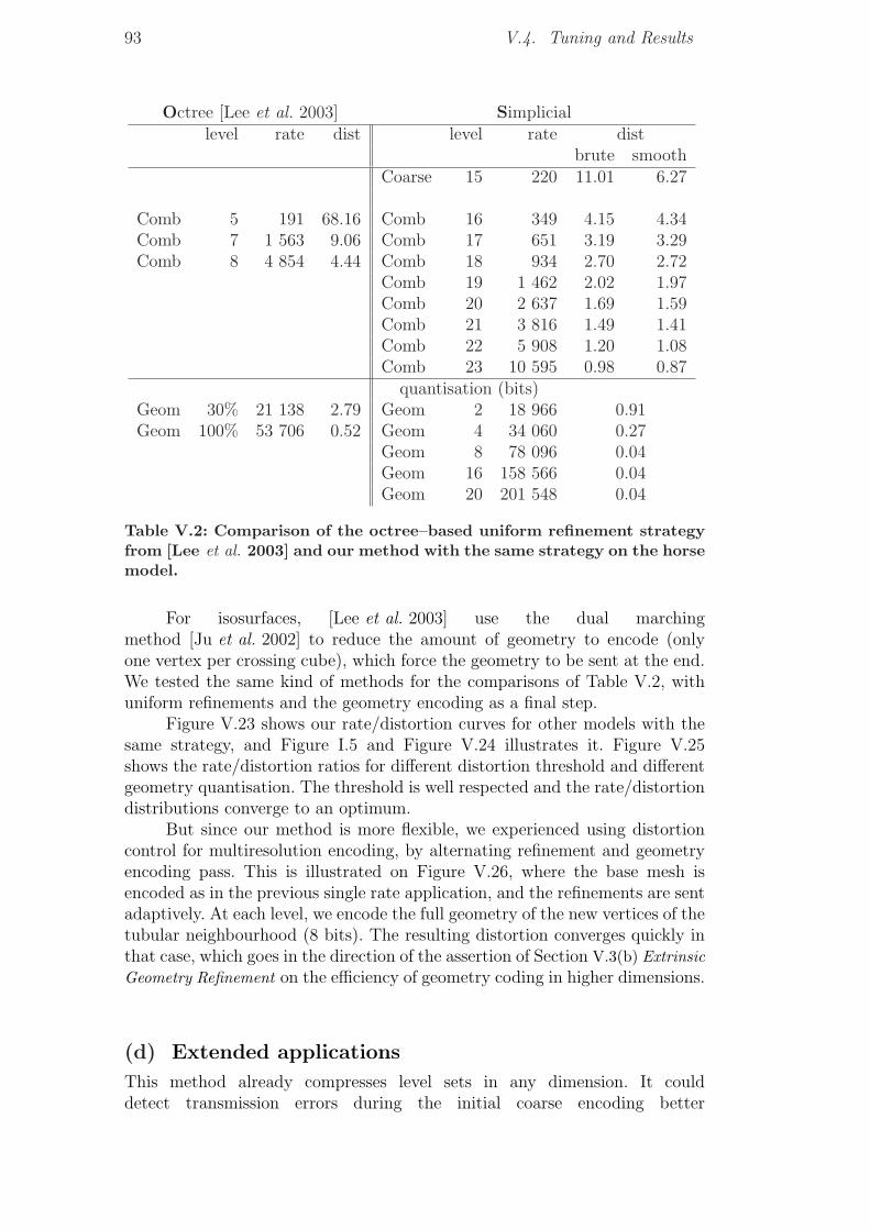
93 V.4. Tuning and Results

Octree [Lee et al. 2003] Simpliciallevel rate dist level rate dist

brute smoothCoarse 15 220 11.01 6.27

Comb 5 191 68.16 Comb 16 349 4.15 4.34Comb 7 1 563 9.06 Comb 17 651 3.19 3.29Comb 8 4 854 4.44 Comb 18 934 2.70 2.72

Comb 19 1 462 2.02 1.97Comb 20 2 637 1.69 1.59Comb 21 3 816 1.49 1.41Comb 22 5 908 1.20 1.08Comb 23 10 595 0.98 0.87

quantisation (bits)Geom 30% 21 138 2.79 Geom 2 18 966 0.91Geom 100% 53 706 0.52 Geom 4 34 060 0.27

Geom 8 78 096 0.04Geom 16 158 566 0.04Geom 20 201 548 0.04

Table V.2: Comparison of the octree–based uniform refinement strategyfrom [Lee et al. 2003] and our method with the same strategy on the horsemodel.

For isosurfaces, [Lee et al. 2003] use the dual marchingmethod [Ju et al. 2002] to reduce the amount of geometry to encode (onlyone vertex per crossing cube), which force the geometry to be sent at the end.We tested the same kind of methods for the comparisons of Table V.2, withuniform refinements and the geometry encoding as a final step.

Figure V.23 shows our rate/distortion curves for other models with thesame strategy, and Figure I.5 and Figure V.24 illustrates it. Figure V.25shows the rate/distortion ratios for different distortion threshold and differentgeometry quantisation. The threshold is well respected and the rate/distortiondistributions converge to an optimum.

But since our method is more flexible, we experienced using distortioncontrol for multiresolution encoding, by alternating refinement and geometryencoding pass. This is illustrated on Figure V.26, where the base mesh isencoded as in the previous single rate application, and the refinements are sentadaptively. At each level, we encode the full geometry of the new vertices of thetubular neighbourhood (8 bits). The resulting distortion converges quickly inthat case, which goes in the direction of the assertion of Section V.3(b) ExtrinsicGeometry Refinement on the efficiency of geometry coding in higher dimensions.

(d) Extended applications

This method already compresses level sets in any dimension. It coulddetect transmission errors during the initial coarse encoding better

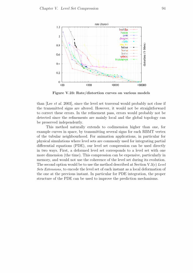
Chapter V. Level Set Compression 94

Figure V.23: Rate/distortion curves on various models

than [Lee et al. 2003], since the level set traversal would probably not close ifthe transmitted signs are altered. However, it would not be straightforwardto correct these errors. In the refinement pass, errors would probably not bedetected since the refinements are mainly local and the global topology canbe preserved independently.

This method naturally extends to codimension higher than one, forexample curves in space, by transmitting several signs for each RBMT vertexof the tubular neighbourhood. For animation applications, in particular forphysical simulations where level sets are commonly used for integrating partialdifferential equations (PDE), our level set compression can be used directlyin two ways. First, a deformed level set corresponds to a level set with onemore dimension (the time). This compression can be expensive, particularly inmemory, and would not use the coherence of the level set during its evolution.The second option would be to use the method described at Section V.3(c) LevelSets Extensions, to encode the level set of each instant as a local deformation ofthe one at the previous instant. In particular for PDE integration, the properstructure of the PDE can be used to improve the prediction mechanisms.

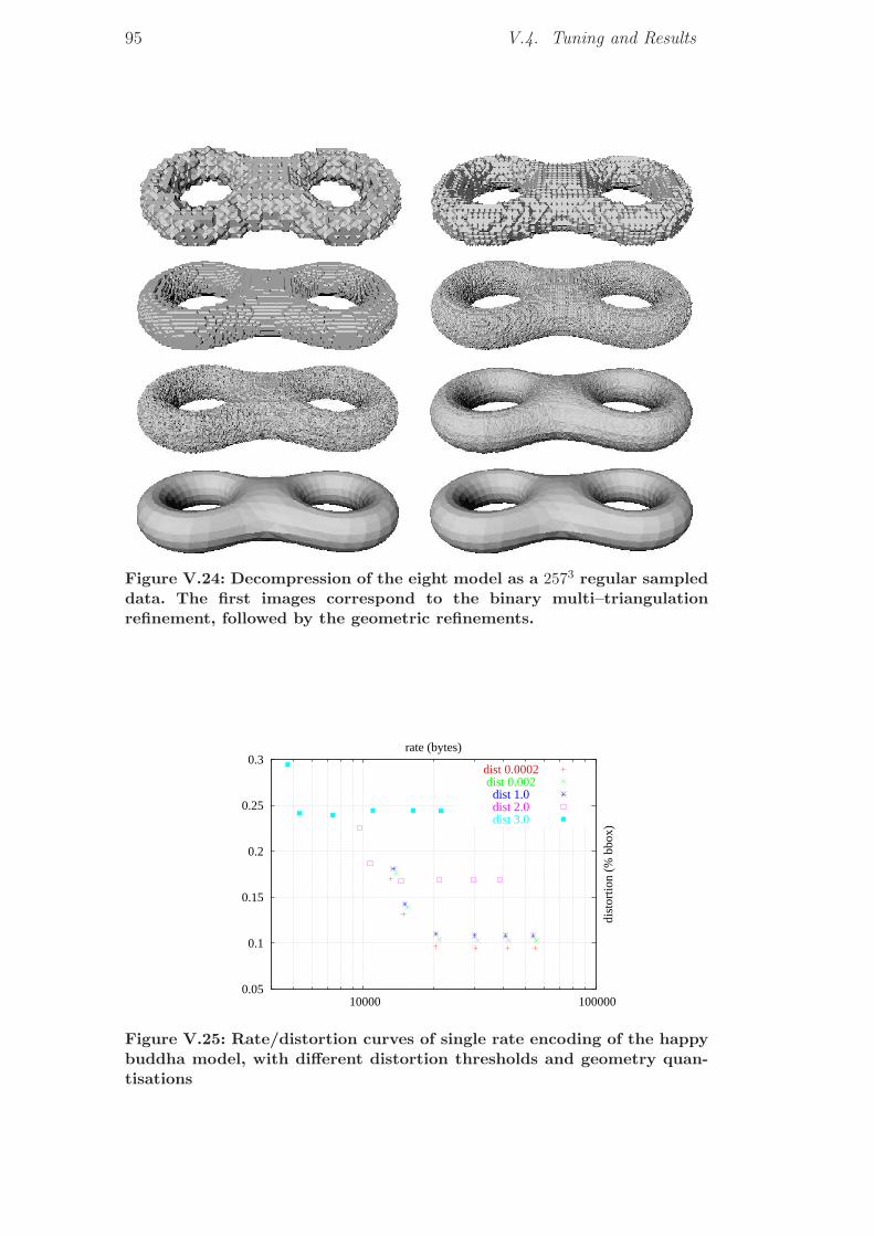
95 V.4. Tuning and Results

Figure V.24: Decompression of the eight model as a 2573 regular sampleddata. The first images correspond to the binary multi–triangulationrefinement, followed by the geometric refinements.

0.05

0.1

0.15

0.2

0.25

0.3

10000 100000

dist

ortio

n (%

bbo

x)

rate (bytes)

dist 0.0002dist 0.002

dist 1.0 dist 2.0 dist 3.0

Figure V.25: Rate/distortion curves of single rate encoding of the happybuddha model, with different distortion thresholds and geometry quan-tisations

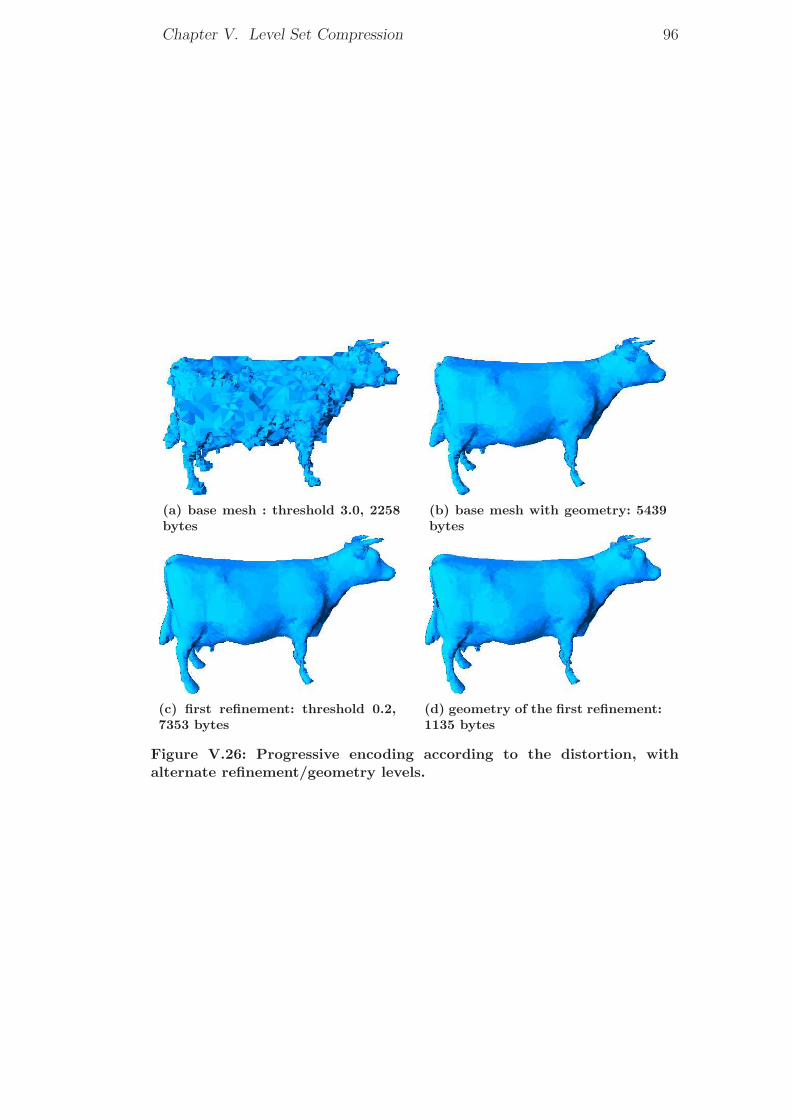
Chapter V. Level Set Compression 96

(a) base mesh : threshold 3.0, 2258bytes

(b) base mesh with geometry: 5439bytes

(c) first refinement: threshold 0.2,7353 bytes

(d) geometry of the first refinement:1135 bytes

Figure V.26: Progressive encoding according to the distortion, withalternate refinement/geometry levels.

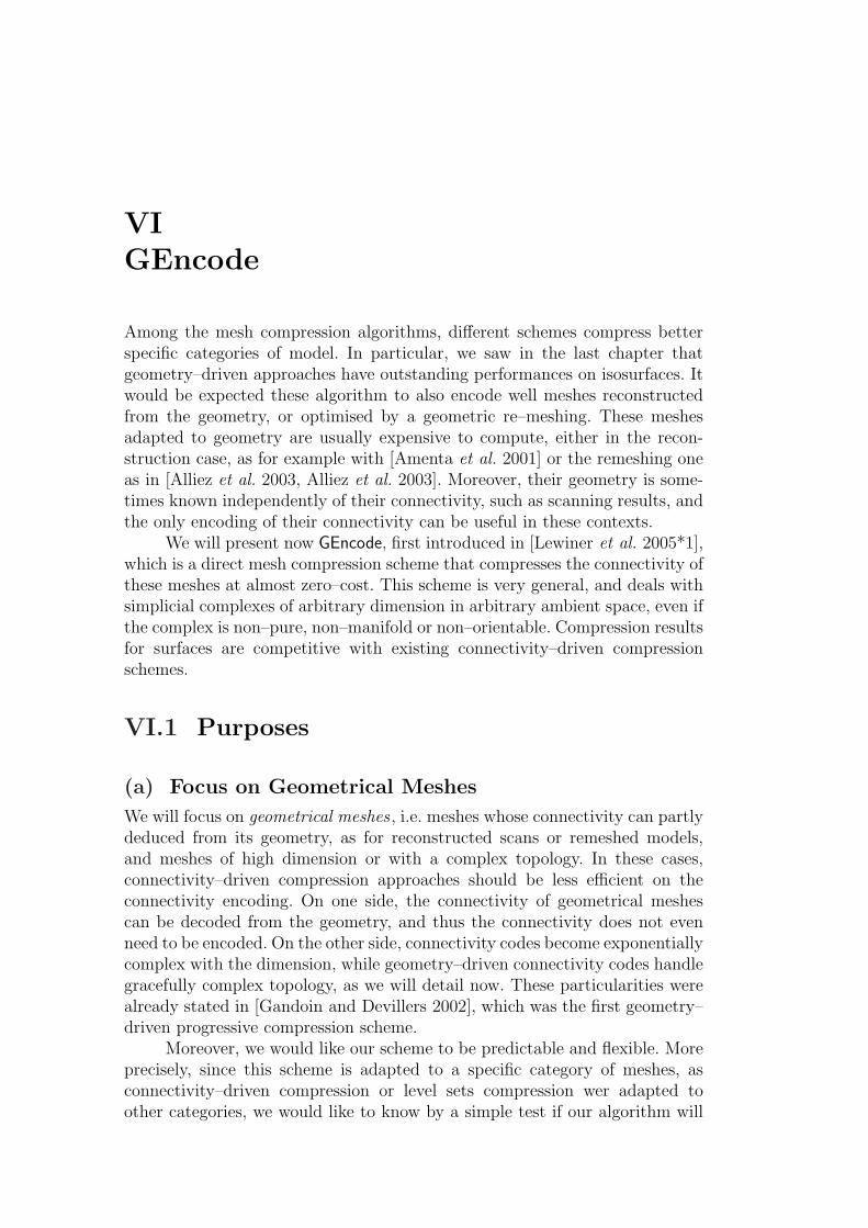
VIGEncode

Among the mesh compression algorithms, different schemes compress betterspecific categories of model. In particular, we saw in the last chapter thatgeometry–driven approaches have outstanding performances on isosurfaces. Itwould be expected these algorithm to also encode well meshes reconstructedfrom the geometry, or optimised by a geometric re–meshing. These meshesadapted to geometry are usually expensive to compute, either in the recon-struction case, as for example with [Amenta et al. 2001] or the remeshing oneas in [Alliez et al. 2003, Alliez et al. 2003]. Moreover, their geometry is some-times known independently of their connectivity, such as scanning results, andthe only encoding of their connectivity can be useful in these contexts.

We will present now GEncode, first introduced in [Lewiner et al. 2005*1],which is a direct mesh compression scheme that compresses the connectivity ofthese meshes at almost zero–cost. This scheme is very general, and deals withsimplicial complexes of arbitrary dimension in arbitrary ambient space, even ifthe complex is non–pure, non–manifold or non–orientable. Compression resultsfor surfaces are competitive with existing connectivity–driven compressionschemes.

VI.1 Purposes

(a) Focus on Geometrical Meshes

We will focus on geometrical meshes , i.e. meshes whose connectivity can partlydeduced from its geometry, as for reconstructed scans or remeshed models,and meshes of high dimension or with a complex topology. In these cases,connectivity–driven compression approaches should be less efficient on theconnectivity encoding. On one side, the connectivity of geometrical meshescan be decoded from the geometry, and thus the connectivity does not evenneed to be encoded. On the other side, connectivity codes become exponentiallycomplex with the dimension, while geometry–driven connectivity codes handlegracefully complex topology, as we will detail now. These particularities werealready stated in [Gandoin and Devillers 2002], which was the first geometry–driven progressive compression scheme.

Moreover, we would like our scheme to be predictable and flexible. Moreprecisely, since this scheme is adapted to a specific category of meshes, asconnectivity–driven compression or level sets compression wer adapted toother categories, we would like to know by a simple test if our algorithm will

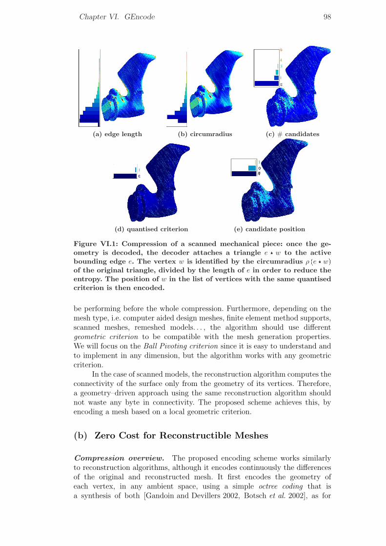
Chapter VI. GEncode 98

(a) edge length (b) circumradius (c) # candidates

(d) quantised criterion (e) candidate position

Figure VI.1: Compression of a scanned mechanical piece: once the ge-ometry is decoded, the decoder attaches a triangle e � w to the activebounding edge e. The vertex w is identified by the circumradius ρ pe � wqof the original triangle, divided by the length of e in order to reduce theentropy. The position of w in the list of vertices with the same quantisedcriterion is then encoded.

be performing before the whole compression. Furthermore, depending on themesh type, i.e. computer aided design meshes, finite element method supports,scanned meshes, remeshed models. . . , the algorithm should use differentgeometric criterion to be compatible with the mesh generation properties.We will focus on the Ball Pivoting criterion since it is easy to understand andto implement in any dimension, but the algorithm works with any geometriccriterion.

In the case of scanned models, the reconstruction algorithm computes theconnectivity of the surface only from the geometry of its vertices. Therefore,a geometry–driven approach using the same reconstruction algorithm shouldnot waste any byte in connectivity. The proposed scheme achieves this, byencoding a mesh based on a local geometric criterion.

(b) Zero Cost for Reconstructible Meshes

Compression overview. The proposed encoding scheme works similarlyto reconstruction algorithms, although it encodes continuously the differencesof the original and reconstructed mesh. It first encodes the geometry ofeach vertex, in any ambient space, using a simple octree coding that isa synthesis of both [Gandoin and Devillers 2002, Botsch et al. 2002], as for

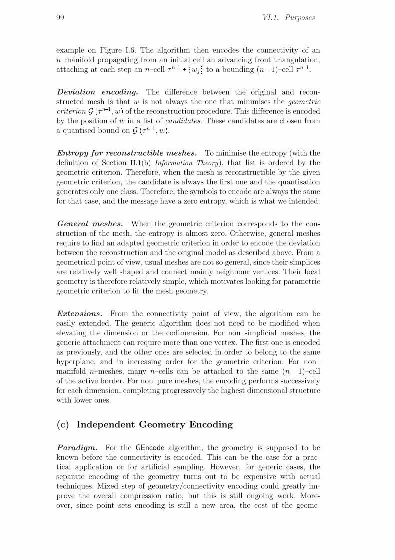
99 VI.1. Purposes

example on Figure I.6. The algorithm then encodes the connectivity of ann–manifold propagating from an initial cell an advancing front triangulation,attaching at each step an n–cell τn�1 � twju to a bounding (n�1)–cell τn�1.

Deviation encoding. The difference between the original and recon-structed mesh is that w is not always the one that minimises the geometriccriterion G pτn�1, wq of the reconstruction procedure. This difference is encodedby the position of w in a list of candidates . These candidates are chosen froma quantised bound on G pτn�1, wq.Entropy for reconstructible meshes. To minimise the entropy (with thedefinition of Section II.1(b) Information Theory), that list is ordered by thegeometric criterion. Therefore, when the mesh is reconstructible by the givengeometric criterion, the candidate is always the first one and the quantisationgenerates only one class. Therefore, the symbols to encode are always the samefor that case, and the message have a zero entropy, which is what we intended.

General meshes. When the geometric criterion corresponds to the con-struction of the mesh, the entropy is almost zero. Otherwise, general meshesrequire to find an adapted geometric criterion in order to encode the deviationbetween the reconstruction and the original model as described above. From ageometrical point of view, usual meshes are not so general, since their simplicesare relatively well shaped and connect mainly neighbour vertices. Their localgeometry is therefore relatively simple, which motivates looking for parametricgeometric criterion to fit the mesh geometry.

Extensions. From the connectivity point of view, the algorithm can beeasily extended. The generic algorithm does not need to be modified whenelevating the dimension or the codimension. For non–simplicial meshes, thegeneric attachment can require more than one vertex. The first one is encodedas previously, and the other ones are selected in order to belong to the samehyperplane, and in increasing order for the geometric criterion. For non–manifold n–meshes, many n–cells can be attached to the same (n� 1)–cellof the active border. For non–pure meshes, the encoding performs successivelyfor each dimension, completing progressively the highest dimensional structurewith lower ones.

(c) Independent Geometry Encoding

Paradigm. For the GEncode algorithm, the geometry is supposed to beknown before the connectivity is encoded. This can be the case for a prac-tical application or for artificial sampling. However, for generic cases, theseparate encoding of the geometry turns out to be expensive with actualtechniques. Mixed step of geometry/connectivity encoding could greatly im-prove the overall compression ratio, but this is still ongoing work. More-over, since point sets encoding is still a new area, the cost of the geome-

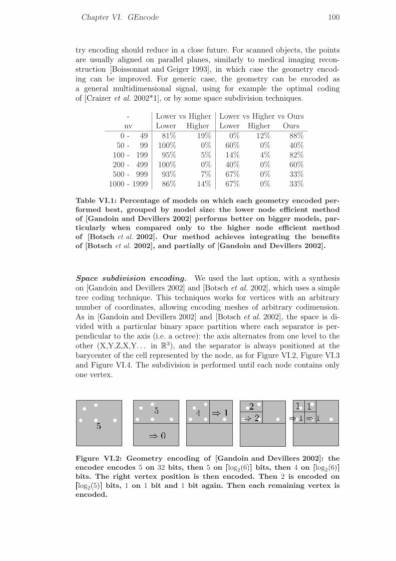
Chapter VI. GEncode 100

try encoding should reduce in a close future. For scanned objects, the pointsare usually aligned on parallel planes, similarly to medical imaging recon-struction [Boissonnat and Geiger 1993], in which case the geometry encod-ing can be improved. For generic case, the geometry can be encoded asa general multidimensional signal, using for example the optimal codingof [Craizer et al. 2002*1], or by some space subdivision techniques.

- Lower vs Higher Lower vs Higher vs Oursnv Lower Higher Lower Higher Ours

0 - 49 81% 19% 0% 12% 88%50 - 99 100% 0% 60% 0% 40%

100 - 199 95% 5% 14% 4% 82%200 - 499 100% 0% 40% 0% 60%500 - 999 93% 7% 67% 0% 33%

1000 - 1999 86% 14% 67% 0% 33%

Table VI.1: Percentage of models on which each geometry encoded per-formed best, grouped by model size: the lower node efficient methodof [Gandoin and Devillers 2002] performs better on bigger models, par-ticularly when compared only to the higher node efficient methodof [Botsch et al. 2002]. Our method achieves integrating the benefitsof [Botsch et al. 2002], and partially of [Gandoin and Devillers 2002].

Space subdivision encoding. We used the last option, with a synthesison [Gandoin and Devillers 2002] and [Botsch et al. 2002], which uses a simpletree coding technique. This techniques works for vertices with an arbitrarynumber of coordinates, allowing encoding meshes of arbitrary codimension.As in [Gandoin and Devillers 2002] and [Botsch et al. 2002], the space is di-vided with a particular binary space partition where each separator is per-pendicular to the axis (i.e. a octree): the axis alternates from one level to theother (X,Y,Z,X,Y. . . in R3), and the separator is always positioned at thebarycenter of the cell represented by the node, as for Figure VI.2, Figure VI.3and Figure VI.4. The subdivision is performed until each node contains onlyone vertex.

Figure VI.2: Geometry encoding of [Gandoin and Devillers 2002]: theencoder encodes 5 on 32 bits, then 5 on rlog2p6qs bits, then 4 on rlog2p6qsbits. The right vertex position is then encoded. Then 2 is encoded onrlog2p5qs bits, 1 on 1 bit and 1 bit again. Then each remaining vertex isencoded.

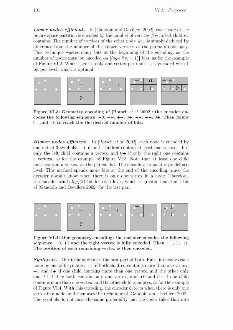
101 VI.1. Purposes

Lower nodes efficient. In [Gandoin and Devillers 2002], each node of thebinary space partition is encoded by the number of vertices #vl its left childrencontains. The number of vertices of the other node #vr is simply deduced bydifference from the number of the known vertices of the parent’s node #vf .This technique wastes many bits at the beginning of the encoding, as thenumber of nodes must be encoded on rlog2p#vf � 1qs bits, as for the exampleof Figure VI.2. When there is only one vertex per node, is is encoded with 1bit per level, which is optimal.

Figure VI.3: Geometry encoding of [Botsch et al. 2002]: the encoder en-codes the following sequence: �0, ��, ��, 0�, ��, ��, 0�. Then follow0� and �0 to reach the the desired number of bits.

Higher nodes efficient. In [Botsch et al. 2002], each node is encoded byone out of 3 symbols: �� if both children contain at least one vertex, �0 ifonly the left child contains a vertex, and 0� if only the right one containsa vertexs, as for the example of Figure VI.3. Note that at least one childmust contain a vertex, as the parent did. The encoding stops at a predefinedlevel. This method spends more bits at the end of the encoding, since thedecoder doesn’t know when there is only one vertex in a node. Therefore,the encoder sends log2p3q bit for each level, which is greater than the 1 bitof [Gandoin and Devillers 2002] for the last part.

Figure VI.4: Our geometry encoding: the encoder encodes the followingsequence: �0, �1 and the right vertex is fully encoded. Then ��, 11, 11.The position of each remaining vertex is then encoded.

Synthesis. Our technique takes the best part of both. First, it encodes eachnode by one of 6 symbols: �� if both children contains more than one vertex,�1 and 1� if one child contains more than one vertex, and the other onlyone, 11 if they both contain only one vertex, and �0 and 0� if one childcontains more than one vertex, and the other child is emptys, as for the exampleof Figure VI.4. With this encoding, the encoder detects when there is only onevertex in a node, and then uses the technique of [Gandoin and Devillers 2002].The symbols do not have the same probability and the coder takes that into

Chapter VI. GEncode 102

account. Moreover, these probabilities are used differently depending on thelevel of the node to encode: nodes closer to the root are more frequently oftype ��, whereas these are rare when going closer to the leaves. For example,the 1986 vertices of the solid sphere of Figure I.6, left, were compressedby [Gandoin and Devillers 2002] with 3433 bytes, by [Botsch et al. 2002] with3877 bytes and by our method with 3429 bytes. The 192 vertices of theCartesian product of a sphere and a circle of Figure I.6, right, were compressedby [Gandoin and Devillers 2002] with 649 bytes, by [Botsch et al. 2002] with980 bytes and by our method with 646 bytes. The coloured lines represent partof the traversal of the mesh by the connectivity encoder.

VI.2 GEncode schemes

(a) Advancing front compression

Any mesh can actually be constructed by a sequence of general attach-ments, as defined in Section III.2(a) Euler Operators. This property is inten-sively used in surface reconstruction with advancing front triangulation algo-rithms [Medeiros et al. 2003], and will be the base of our algorithm. The meshis built step by step, each step consisting in attaching a cell to the boundary ofthe last step, called the active boundary . The cell attached is the join of a cellτn�1 of the active boundary with some vertices wi. For example for triangulatedsurfaces, the triangle attached is the join of an edge of the active boundarywith one vertex. Since the geometry of all the vertices is known, the problem isto identify which vertices wi are used for the attachment, and we will identifyeach wi by its position j inside a list of candidates : wj P tv1, . . . , vku. Thisprocess is implemented by Algorithm 15: gencode and Algorithm 16: gdecode.For these algorithms, we suppose that there is at most one cell spanning agiven set of vertices.

(b) Optimisations and Extensions

Generality of GEncode. The above algorithms are actually very general,and can be simplified for specific cases. In its present forms, it handlessimplicial complexes and polytopes of arbitrary dimension, embedded in anycodimensional space. The complex can be orientable or not, and have any kindof topology. It can respect the manifold or pseudo–manifold criterion or not.We will see how each of these restrictions can simplify the algorithm, andimprove the final compression ration. Such improvements do not change thenature of the GEncode, but accelerates its execution. For example, we can pushonly the unmarked n�1–cells of the frontier of the attached cells at lines 33and 29 of Algorithm 15: gencode and Algorithm 16: gdecode respectively, inorder to maintain a smaller priority queue and to avoid the test of lines 7and 6 of Algorithm 15: gencode and Algorithm 16: gdecode respectively.

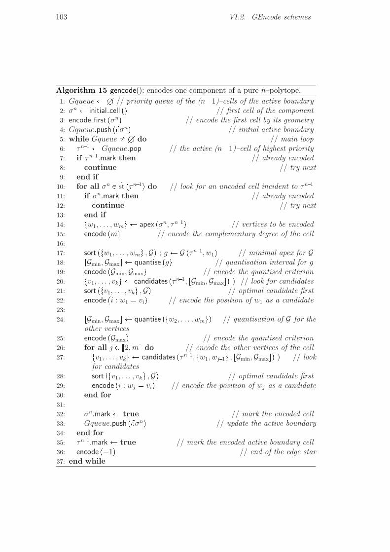
103 VI.2. GEncode schemes

Algorithm 15 gencode(): encodes one component of a pure n–polytope.

1: Gqueue ÐH // priority queue of the (n�1)–cells of the active boundary2: σn Ð initial cell pq // first cell of the component3: encode first pσnq // encode the first cell by its geometry4: Gqueue.push pBσnq // initial active boundary5: while Gqueue � H do // main loop6: τn�1 Ð Gqueue.pop // the active (n�1)–cell of highest priority7: if τn�1.mark then // already encoded8: continue // try next9: end if

10: for all σn P 9st pτn�1q do // look for an uncoded cell incident to τn�111: if σn.mark then // already encoded12: continue // try next13: end if14: tw1, . . . , wmu Ð apex pσn, τn�1q // vertices to be encoded15: encode pmq // encode the complementary degree of the cell16:17: sort ptw1, . . . , wmu ,Gq ; g Ð G pτn�1, w1q // minimal apex for G18: rGmin,Gmaxs Ð quantise pgq // quantisation interval for g19: encode pGmin,Gmaxq // encode the quantised criterion20: tv1, . . . , vku Ð candidates pτn�1, rGmin,Gmaxsq ) // look for candidates21: sort ptv1, . . . , vku ,Gq // optimal candidate first22: encode pi : w1 � viq // encode the position of w1 as a candidate23:24: rGmin,Gmaxs Ð quantise ptw2, . . . , wmuq // quantisation of G for the

other vertices25: encode pGmaxq // encode the quantised criterion26: for all j P v2,mw do // encode the other vertices of the cell27: tv1, . . . , vku Ð candidates pτn�1, tw1, wj�1u , rGmin,Gmaxsq ) // look

for candidates28: sort ptv1, . . . , vku ,Gq // optimal candidate first29: encode pi : wj � viq // encode the position of wj as a candidate30: end for31:32: σn.mark Ð true // mark the encoded cell33: Gqueue.push pBσnq // update the active boundary34: end for35: τn�1.mark Ð true // mark the encoded active boundary cell36: encode p�1q // end of the edge star37: end while

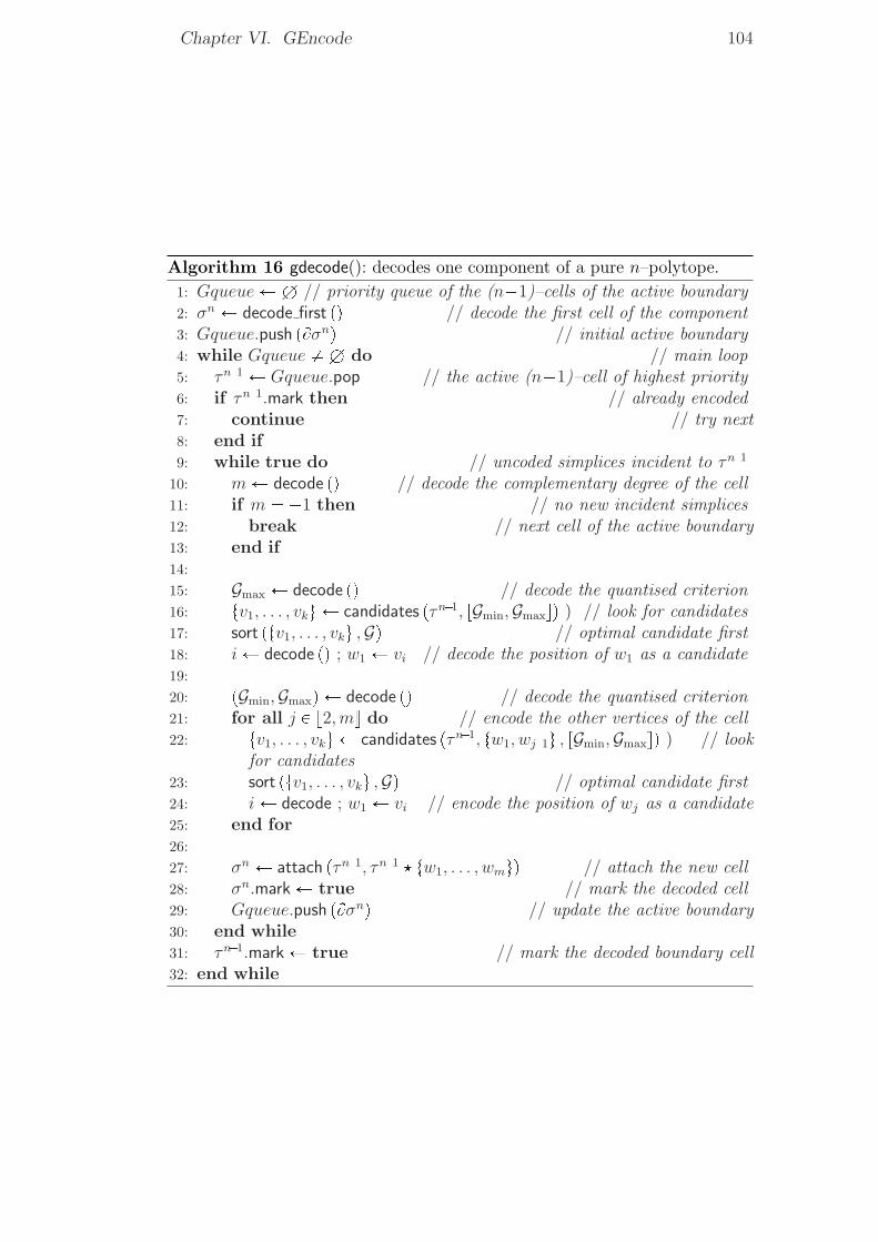
Chapter VI. GEncode 104

Algorithm 16 gdecode(): decodes one component of a pure n–polytope.

1: Gqueue ÐH // priority queue of the (n�1)–cells of the active boundary2: σn Ð decode first pq // decode the first cell of the component3: Gqueue.push pBσnq // initial active boundary4: while Gqueue � H do // main loop5: τn�1 Ð Gqueue.pop // the active (n�1)–cell of highest priority6: if τn�1.mark then // already encoded7: continue // try next8: end if9: while true do // uncoded simplices incident to τn�1

10: m Ð decode pq // decode the complementary degree of the cell11: if m � �1 then // no new incident simplices12: break // next cell of the active boundary13: end if14:15: Gmax Ð decode pq // decode the quantised criterion16: tv1, . . . , vku Ð candidates pτn�1, rGmin,Gmaxsq ) // look for candidates17: sort ptv1, . . . , vku ,Gq // optimal candidate first18: i Ð decode pq ; w1 Ð vi // decode the position of w1 as a candidate19:20: pGmin,Gmaxq Ð decode pq // decode the quantised criterion21: for all j P v2,mw do // encode the other vertices of the cell22: tv1, . . . , vku Ð candidates pτn�1, tw1, wj�1u , rGmin,Gmaxsq ) // look

for candidates23: sort ptv1, . . . , vku ,Gq // optimal candidate first24: i Ð decode ; w1 Ð vi // encode the position of wj as a candidate25: end for26:27: σn Ð attach pτn�1, τn�1 � tw1, . . . , wmuq // attach the new cell28: σn.mark Ð true // mark the decoded cell29: Gqueue.push pBσnq // update the active boundary30: end while31: τn�1.mark Ð true // mark the decoded boundary cell32: end while

105 VI.2. GEncode schemes

Simplicial meshes. For simplicial meshes, we know that each n–simplexhas n�1 vertices. Therefore the m symbol is always equal to 1 at lines 15and 10 of Algorithm 15: gencode and Algorithm 16: gdecode respectively. More-over, the coding of the extra vertices tw2, wm�1u can be avoided, which sup-presses lines 16 to 31 of Algorithm 15: gencode, and lines 19 to 26 of Algo-rithm 16: gdecode. For generic purposes, this can be implemented with thesame algorithms by incorporating this information in the probability modelof the m symbols, either at initialisation or progressively, as described in Sec-tion II.2(c) Statistical Modelling.

Manifolds. If the mesh is a pseudo–manifold with an empty border, weknow that each n�1–cell is incident to exactly two n–cells. Therefore, there isno need to encode the �1 symbol at lines 36 and 11 of Algorithm 15: gencode

and Algorithm 16: gdecode respectively, nor to include the loops starting atlines 10 and 9 of Algorithm 15: gencode and Algorithm 16: gdecode respectively,that wait for this symbol. Furthermore, if we know the original mesh ismanifold, we can remove from the list the candidates that would create anon–manifold mesh, i.e. the vertices that are not in the active boundary.

Non–pure complexes. The above algorithms can be easily extendedto handle multiple components and non–pure elements by calling Algo-rithm 15: gencode and Algorithm 16: gdecode many times. For the first case, thealgorithm is called once per component using the function initial cell at line 2of Algorithm 15: gencode, and a by encoding a bit signal Stop/Continue at theend of the procedure. Non–pure elements of dimension p   n, i.e. p–cells notface of any (p�1)–cell, can actually be considered as pure elements of the p–skeleton Kppq, as defined at Section III.1(a) Simplicial Complexes. The algorithmthen encodes the pure part Kpure of the polytope with Algorithm 15: gencode,and then successively encodes the pure parts Kpureppq of the lower skeletons Kppq,starting with the boundary of Kpurepp�1q as active boundary, and considering each

cell of Kpurepp�1q as already encoded. This involves at most n�1 calls to Algo-rithm 15: gencode or Algorithm 16: gdecode.

(c) Candidates selection

Quantisation. The decoder has to choose which vertices w of the encodedmesh was adjacent to τn�1. This information is encoded by the index of winside a list of candidates. This list could be the list of all vertices, but thatwould require O plog p#0qq bits for each vertex, which is too expensive. In orderto minimise the number of elements of the candidate list and the time usedto create that list, the geometric criterion G pτn�1, wq of w is quantised andencoded. This quantisation is a tradeoff: On one hand, if the quantisation isbrutal, there will be many candidates, which means a long time to generatethe list and an expensive encoding of the position of w in the list of thecandidates, as show the histograms of Figure VI.5. On the other hand, if thequantisation is too refined, the quantised geometric criterion will be expensive

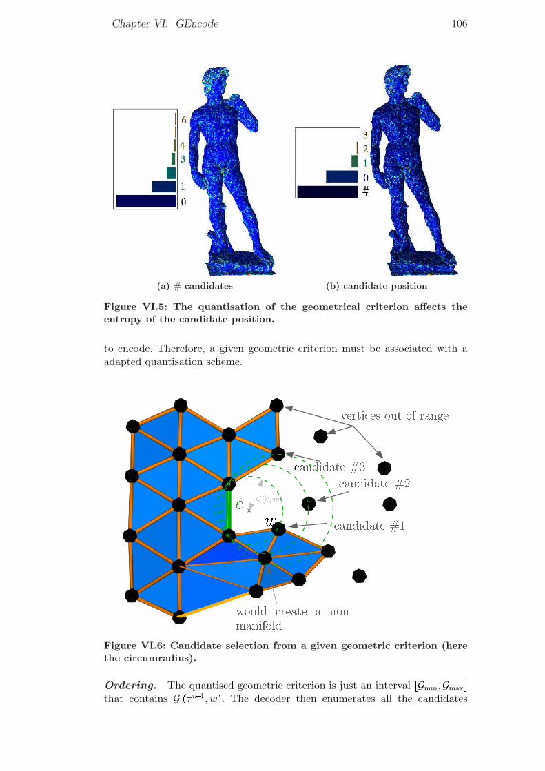
Chapter VI. GEncode 106

(a) # candidates (b) candidate position

Figure VI.5: The quantisation of the geometrical criterion affects theentropy of the candidate position.

to encode. Therefore, a given geometric criterion must be associated with aadapted quantisation scheme.

Figure VI.6: Candidate selection from a given geometric criterion (herethe circumradius).

Ordering. The quantised geometric criterion is just an interval rGmin,Gmaxsthat contains G pτn�1, wq. The decoder then enumerates all the candidates

107 VI.3. Geometric Criteria

vi R τn�1 that could fit in this interval : G pτn�1, viq P rGmin,Gmaxs, and order thislist of candidates by G: G pτn�1, viq   G pτn�1, vi�1q, as shown on Figure VI.6.For typical meshes, this ordering lowers drastically the entropy, since the vertexw is usually one of the first ones, and the entropy coder can reflect this usingpredefined probabilities, as described in Section II.2(c) Statistical Modelling.

Non–simplicial meshes. In the implementation, the binary space parti-tion created by the encoding of the geometry is used to accelerate the searchfor candidates, when the range of the geometric criterion can be bound inthe ambient space. However, the number of candidates for the other verticestw2, wm�1u can be further reduced : On one hand, these vertices belong to thehyperplane containing τn�1 � w, and not to the hyperplane supporting τn�1.This criterion translates directly on the binary space partition, and greatly ac-celerates the search. On the other hand, the vertices wj are taken in increasingorder of G, which means that the lower bound of the quantisation interval isreduced at each step.

VI.3 Geometric Criteria

For reconstruction purposes, the vertex w chosen to join the simplex τn�1

minimises a geometric criterion G pτn�1, wq � Gmin pτn�1q. For example, theBall Pivoting Algorithm of [Bernardini et al. 1999, Medeiros et al. 2004] usesthe circumradius of the simplex τn�1 � w as geometric criterion: G pτn�1, wq �ρ pτn�1 � wq.

This geometric criterion is a fundamental piece of the GEncode scheme,since it must predict the local rules to deduce the connectivity from thegeometry. In this section, we will describe which are the important elementsof a geometric criterion, and detail these by the specific example of a criterionderived from the Ball Pivoting Algorithm. We will conclude by some indicationsto a practical scheme for deducing a ad hoc criterion for a given mesh.

(a) Generic Formulation

Purpose. Consider a fixed mesh K. A geometric criterion is a real valuedfunction G pτn�1, wq depending on an active (n�1)–simplex τn�1, a candidatevertex w and eventually any vertex of the complete mesh and the alreadydecoded mesh. The geometry criterion is adapted to K if, for a fixed activesimplex τn�1, this function assigns the lowest possible values to the apex w ofan n–simplex τn�1�w of K. This would characterise the mesh local connectivityfrom its geometry, but for practical use in our GEncode scheme, the criterionmust satisfy other

Quantisation/enumeration tradeoff. In order to avoid generating hugelists of candidates, the geometric criterion is quantised into a few classes. Thisquantisation should optimise the tradeoff between the number of candidatesgenerated and the number of classes. A simple class repartition mechanism

Chapter VI. GEncode 108

would be an exponential increase of the class size, giving more precision for themore frequent elements. However, this should be specified for each geometriccriterion.

Spatial extension. The search for candidates can be accelerated using thebinary space partition created by the encoding of the geometry describedat Section VI.1(c) Independent Geometry Encoding. To do so, a range of thegeometric criterion should correspond to a spatial restriction, in order to lookfor candidates in only a specific part of the space. This generates a significantacceleration of the algorithm.

Traversal strategy. The geometric configuration of a simplex σn differs iflooking at it from an apex w (σn � τ � w) or another one w1 (σn � τ 1 � w1),as shown on Figure VI.8. The geometric criterion can perform better ifentering in a simplex σn by a specific face τn�1. That is why the activeboundary is implemented by a priority queue in Algorithm 15: gencode

and Algorithm 16: gdecode. The geometric criterion can thus be enhanced bya specific priority for the faces of the active boundary.

(b) Ball–Pivoting and Delaunay–Based Reconstruction

Delaunay–based meshes. In order to illustrate the GEncode schemewith a practical geometric criterion, we will present a criterion derived fromthe simple and efficient reconstruction algorithm of [Bernardini et al. 1999]:the Ball Pivoting described at Section III.3(b) Delaunay Triangulation. Formeshes that were reconstructed with this algorithm, or with similarDelaunay–based reconstruction algorithms as [Boissonnat and Geiger 1993,Lopes et al. 2000, Chaine and Bouakaz 2000, Boissonnat and Cazals 2002,Cohen–Steiner and Da 2002, Nonato et al. 2005], this criterion will be partic-ularly efficient.

Ball Pivoting criterion. For surfaces, the Ball Pivoting algorithm alwaysattaches to an active boundary edge τ 1 the vertex w that minimizes thecircumradius ρ ptq of the triangle t � τ 1 � w. This can be extended tohigher dimensions, as was done in [Medeiros et al. 2004]. The circumradiuscan be computed in high dimensions using derivations of the Cayley–Mengerdeterminant [Blumenthal 1970]. In practise, this computation is expensive, andcan be substituted by the volume |σ| of σ � τn�1�w, using directly the Cayley–Menger determinant.

Quantisation. The quantisation can actually be improved if we consider thecircumradius divided by the length of the active face as show the histogramsof Figure VI.7 :

G �τn�1, w� � ρpτn�1�wq|τn�1| .

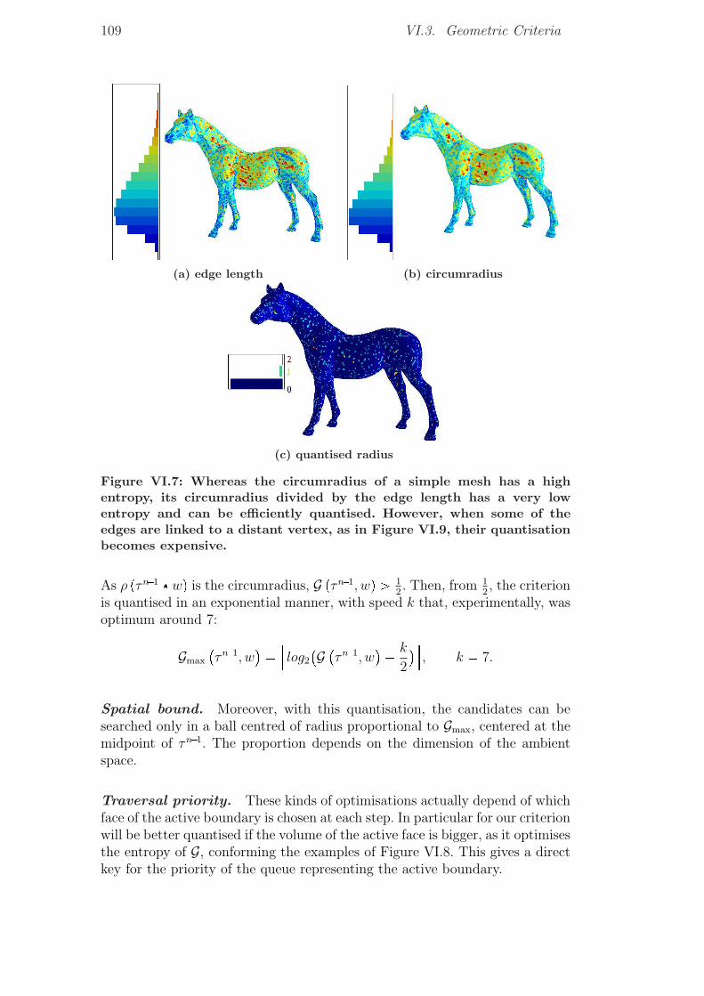
109 VI.3. Geometric Criteria

(a) edge length (b) circumradius

(c) quantised radius

Figure VI.7: Whereas the circumradius of a simple mesh has a highentropy, its circumradius divided by the edge length has a very lowentropy and can be efficiently quantised. However, when some of theedges are linked to a distant vertex, as in Figure VI.9, their quantisationbecomes expensive.

As ρ pτn�1 � wq is the circumradius, G pτn�1, wq ¡ 12. Then, from 1

2, the criterion

is quantised in an exponential manner, with speed k that, experimentally, wasoptimum around 7:

Gmax

�τn�1, w� � Q

log2

�G �τn�1, w�� k

2

�U, k � 7.

Spatial bound. Moreover, with this quantisation, the candidates can besearched only in a ball centred of radius proportional to Gmax, centered at themidpoint of τn�1. The proportion depends on the dimension of the ambientspace.

Traversal priority. These kinds of optimisations actually depend of whichface of the active boundary is chosen at each step. In particular for our criterionwill be better quantised if the volume of the active face is bigger, as it optimisesthe entropy of G, conforming the examples of Figure VI.8. This gives a directkey for the priority of the queue representing the active boundary.

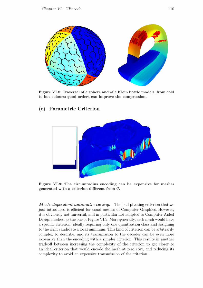
Chapter VI. GEncode 110

Figure VI.8: Traversal of a sphere and of a Klein bottle models, from coldto hot colours: good orders can improve the compression.

(c) Parametric Criterion

Figure VI.9: The circumradius encoding can be expensive for meshesgenerated with a criterion different from G.

Mesh–dependent automatic tuning. The ball pivoting criterion that wejust introduced is efficient for usual meshes of Computer Graphics. However,it is obviously not universal, and in particular not adapted to Computer AidedDesign meshes, as the one of Figure VI.9. More generally, each mesh would havea specific criterion, ideally requiring only one quantisation class and assigningto the right candidate a local minimum. This kind of criterion can be arbitrarilycomplex to describe, and its transmission to the decoder can be even moreexpensive than the encoding with a simpler criterion. This results in anothertradeoff between increasing the complexity of the criterion to get closer toan ideal criterion that would encode the mesh at zero cost, and reducing itscomplexity to avoid an expensive transmission of the criterion.

111 VI.3. Geometric Criteria

Parametric criterion. Actually, for a given mesh and eventually a giventraversal of the mesh, we can create a sampling of the criterion G : Rnd�Rd ÑR by assigning to each gate τn�1 one sample per valid vertex w of the mesh. Avertex is valid if it does not create a degenerated cell, and for the manifold case,if it belongs to the active boundary during the traversal. The gate is consideredas a simplex by eventually omitting some vertices, in order to simplify thesampling task. The domain of the criterion is actually projected in order toput the gate τn�1 at the origin and aligned with the axes. The real valueassociated with the sample pτn�1, wq is somehow arbitrary, and can be 0 if thevertex is the apex of a valid cell of the mesh, and 1 otherwise. This value canbe scaled by the distance of the vertex to the gate in order to get a better fit,and far–away vertices can be omitted to accelerate the process. The criterionis then a parametric fit of these samples, for example using [Pratt 1987]. Forexample, a low–degree polynomial or rational fraction can be used, which wouldencompass the Ball Pivoting criterion.

Quantised class creation. The quantisation can be directly deduced bysumming for each value of the criterion the position of the right apex foreach gate inside the list of candidates of higher criterion. The quantisationcan optimally allocate quantisation intervals to have the lowest average valueinside each class.

Spatial division. We can compute the maximal distance of a valid vertexto the centre of a gate directly for each quantisation bound. This informationcan be transmitted directly since there are only a few quantisation intervals.Eventually, these distances are affected by the volume of the gate, which canbe taken in account here, similarly to the Ball Pivoting criterion.

Traversal guiding. The traversal strategy is somehow harder to deduceautomatically, mainly because the whole criterion depends on the traversal.Since the traversal should be guided by only the gates, we should start withone priority for a gate, such as the volume or the orientation, and draw theerror of the criterion as a function of that priority function. Then, a simpletransformation, such as a multiplication by �1 or a recentring on an intervalra, bs (x ÞÑ px� aq pb� xq), can outline a lower error on higher value of thetransformed priority. If the difference between low and high values is notsignificant, another priority could be used.

Practical use. This method is time consuming in practise, which preventsits direct use for each mesh to encode. However, it can be used to generatecriteria for a specific class of meshes. For example, this process can be appliedto a sequence of meshes generated for a specific finite element method. Theresulting criterion would then be hard coded to form a specific compressionalgorithm for this kind of meshes. The only care to be taken concerns the spatialextension, which should either be guaranteed, or the algorithm should take inaccount escape codes to handle exceptions to the extension rules. Moreover,

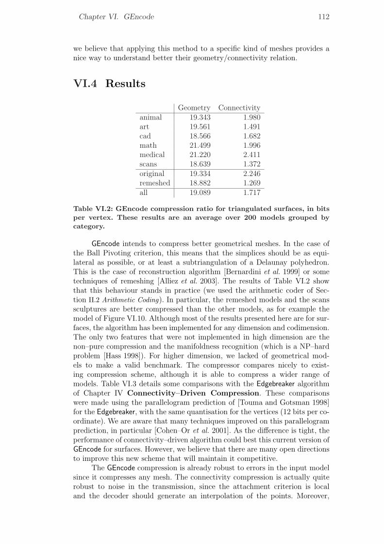
Chapter VI. GEncode 112

we believe that applying this method to a specific kind of meshes provides anice way to understand better their geometry/connectivity relation.

VI.4 Results

Geometry Connectivityanimal 19.343 1.980art 19.561 1.491cad 18.566 1.682math 21.499 1.996medical 21.220 2.411scans 18.639 1.372original 19.334 2.246remeshed 18.882 1.269all 19.089 1.717

Table VI.2: GEncode compression ratio for triangulated surfaces, in bitsper vertex. These results are an average over 200 models grouped bycategory.

GEncode intends to compress better geometrical meshes. In the case ofthe Ball Pivoting criterion, this means that the simplices should be as equi-lateral as possible, or at least a subtriangulation of a Delaunay polyhedron.This is the case of reconstruction algorithm [Bernardini et al. 1999] or sometechniques of remeshing [Alliez et al. 2003]. The results of Table VI.2 showthat this behaviour stands in practice (we used the arithmetic coder of Sec-tion II.2 Arithmetic Coding). In particular, the remeshed models and the scanssculptures are better compressed than the other models, as for example themodel of Figure VI.10. Although most of the results presented here are for sur-faces, the algorithm has been implemented for any dimension and codimension.The only two features that were not implemented in high dimension are thenon–pure compression and the manifoldness recognition (which is a NP–hardproblem [Hass 1998]). For higher dimension, we lacked of geometrical mod-els to make a valid benchmark. The compressor compares nicely to exist-ing compression scheme, although it is able to compress a wider range ofmodels. Table VI.3 details some comparisons with the Edgebreaker algorithmof Chapter IV Connectivity–Driven Compression. These comparisonswere made using the parallelogram prediction of [Touma and Gotsman 1998]for the Edgebreaker, with the same quantisation for the vertices (12 bits per co-ordinate). We are aware that many techniques improved on this parallelogramprediction, in particular [Cohen–Or et al. 2001]. As the difference is tight, theperformance of connectivity–driven algorithm could best this current version ofGEncode for surfaces. However, we believe that there are many open directionsto improve this new scheme that will maintain it competitive.

The GEncode compression is already robust to errors in the input modelsince it compresses any mesh. The connectivity compression is actually quiterobust to noise in the transmission, since the attachment criterion is localand the decoder should generate an interpolation of the points. Moreover,

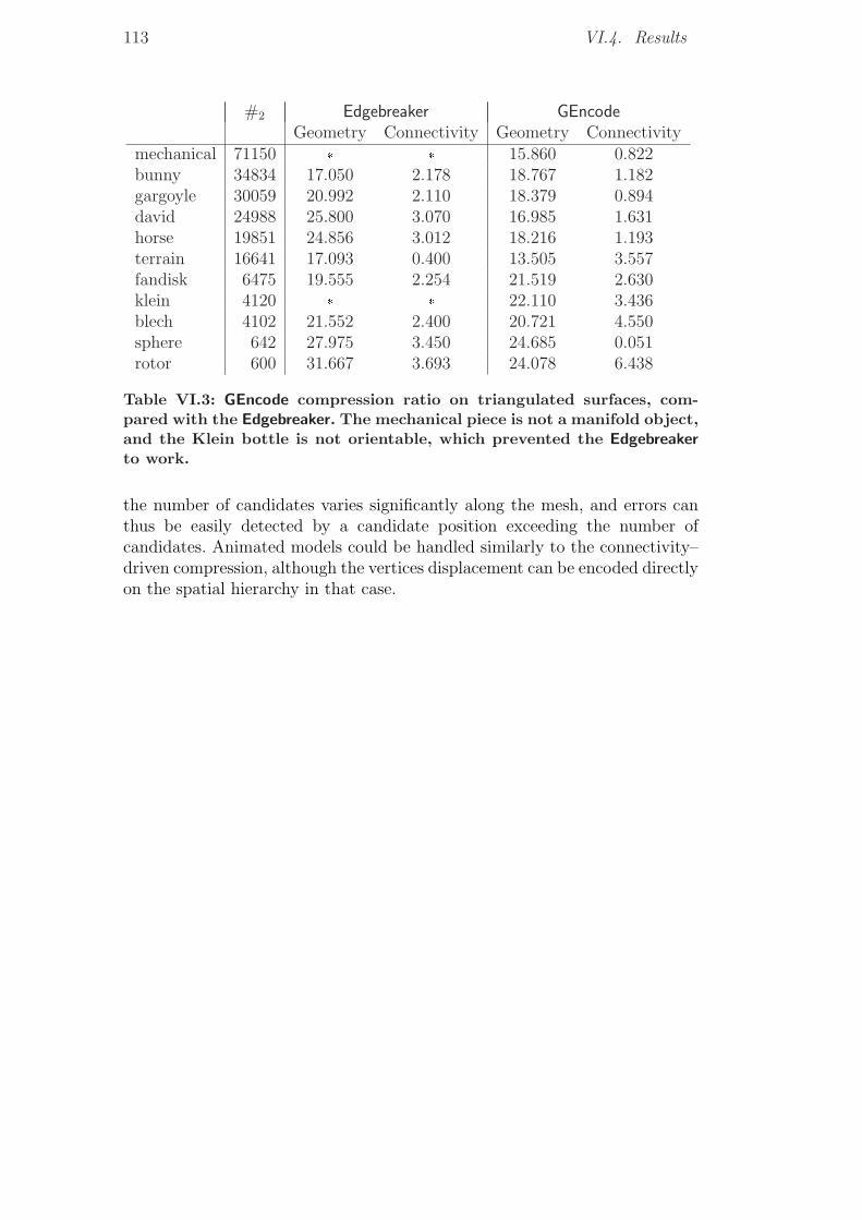
113 VI.4. Results

#2 Edgebreaker GEncodeGeometry Connectivity Geometry Connectivity

mechanical 71150 � � 15.860 0.822bunny 34834 17.050 2.178 18.767 1.182gargoyle 30059 20.992 2.110 18.379 0.894david 24988 25.800 3.070 16.985 1.631horse 19851 24.856 3.012 18.216 1.193terrain 16641 17.093 0.400 13.505 3.557fandisk 6475 19.555 2.254 21.519 2.630klein 4120 � � 22.110 3.436blech 4102 21.552 2.400 20.721 4.550sphere 642 27.975 3.450 24.685 0.051rotor 600 31.667 3.693 24.078 6.438

Table VI.3: GEncode compression ratio on triangulated surfaces, com-pared with the Edgebreaker. The mechanical piece is not a manifold object,and the Klein bottle is not orientable, which prevented the Edgebreakerto work.

the number of candidates varies significantly along the mesh, and errors canthus be easily detected by a candidate position exceeding the number ofcandidates. Animated models could be handled similarly to the connectivity–driven compression, although the vertices displacement can be encoded directlyon the spatial hierarchy in that case.

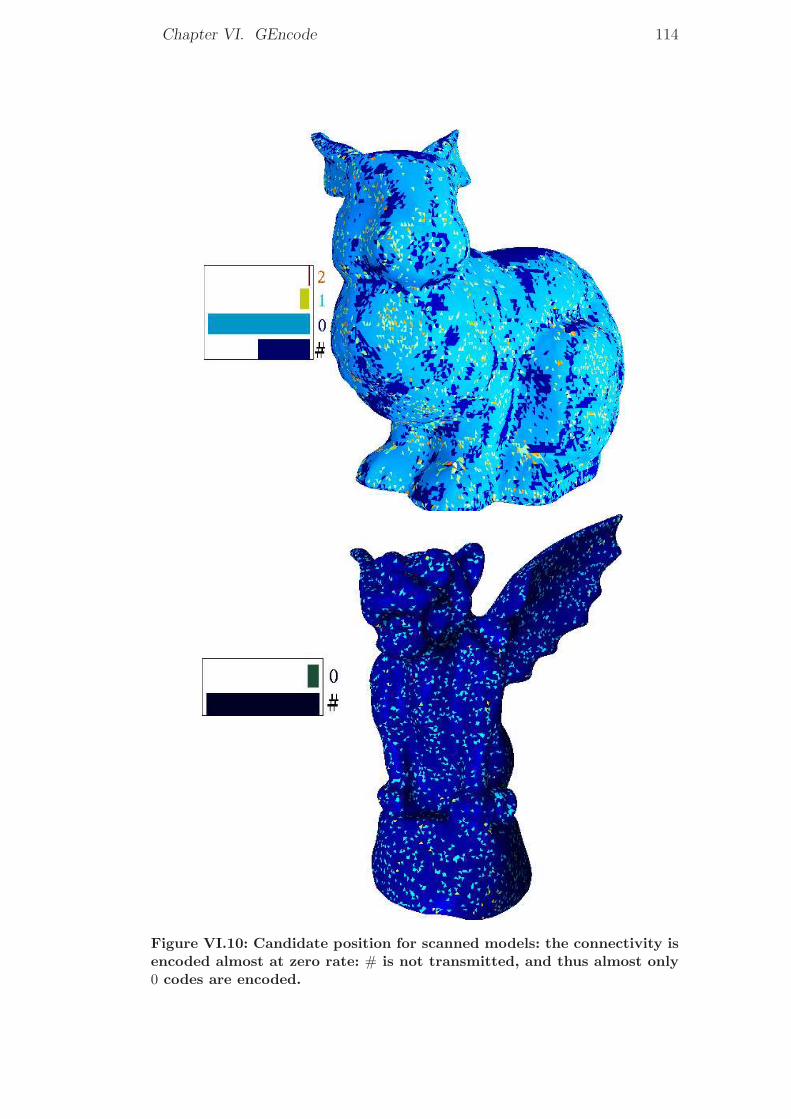
Chapter VI. GEncode 114

Figure VI.10: Candidate position for scanned models: the connectivity isencoded almost at zero rate: # is not transmitted, and thus almost only0 codes are encoded.

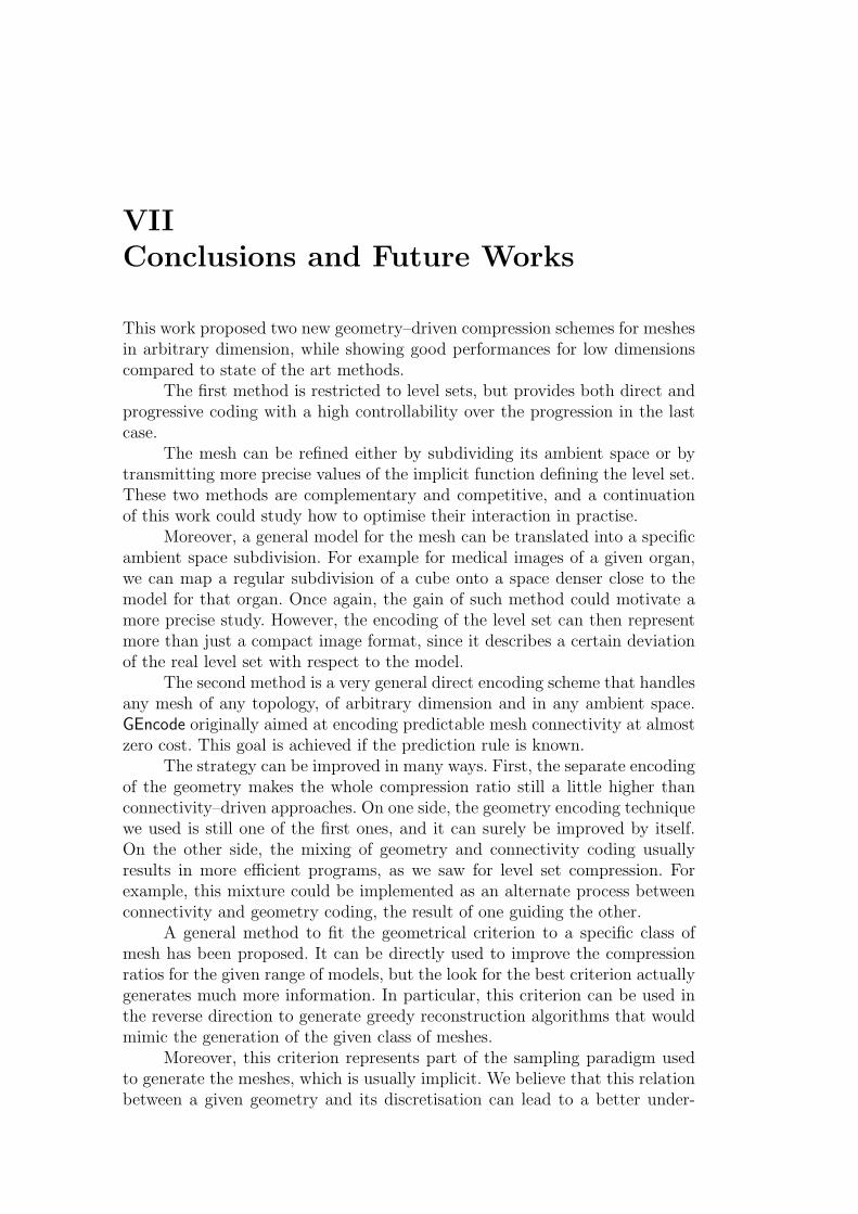
VIIConclusions and Future Works

This work proposed two new geometry–driven compression schemes for meshesin arbitrary dimension, while showing good performances for low dimensionscompared to state of the art methods.

The first method is restricted to level sets, but provides both direct andprogressive coding with a high controllability over the progression in the lastcase.

The mesh can be refined either by subdividing its ambient space or bytransmitting more precise values of the implicit function defining the level set.These two methods are complementary and competitive, and a continuationof this work could study how to optimise their interaction in practise.

Moreover, a general model for the mesh can be translated into a specificambient space subdivision. For example for medical images of a given organ,we can map a regular subdivision of a cube onto a space denser close to themodel for that organ. Once again, the gain of such method could motivate amore precise study. However, the encoding of the level set can then representmore than just a compact image format, since it describes a certain deviationof the real level set with respect to the model.

The second method is a very general direct encoding scheme that handlesany mesh of any topology, of arbitrary dimension and in any ambient space.GEncode originally aimed at encoding predictable mesh connectivity at almostzero cost. This goal is achieved if the prediction rule is known.

The strategy can be improved in many ways. First, the separate encodingof the geometry makes the whole compression ratio still a little higher thanconnectivity–driven approaches. On one side, the geometry encoding techniquewe used is still one of the first ones, and it can surely be improved by itself.On the other side, the mixing of geometry and connectivity coding usuallyresults in more efficient programs, as we saw for level set compression. Forexample, this mixture could be implemented as an alternate process betweenconnectivity and geometry coding, the result of one guiding the other.

A general method to fit the geometrical criterion to a specific class ofmesh has been proposed. It can be directly used to improve the compressionratios for the given range of models, but the look for the best criterion actuallygenerates much more information. In particular, this criterion can be used inthe reverse direction to generate greedy reconstruction algorithms that wouldmimic the generation of the given class of meshes.

Moreover, this criterion represents part of the sampling paradigm usedto generate the meshes, which is usually implicit. We believe that this relationbetween a given geometry and its discretisation can lead to a better under-

Chapter VII. Conclusions and Future Works 116

standing of discrete geometry. Designing coding schemes actually translatesinto isolating and representing clearly the most relevant information of the ob-jects to encode. In that sense, it provides a nice framework to approach theseessential questions.

These two geometry–driven methods are general, and compare nicely toexisting surface compression schemes. In particular for isosurfaces, our methodimproved on state–of–the–art methods, which already outperformed genericsurface compression schemes. For more general surfaces, GEncode comparesnicely to the Edgebreaker. However, these two approaches are delicate tocompare. On one side, the geometry coding of GEncode is more adapted toregular sampling in the space, and the one of the Edgebreaker relies on theregularity of the sampling on the surface. On the other side, the local coherenceof the sampling is directly used in the contexts of the arithmetic coder forthe octree coding, whereas this coherence is included in the parallelogramprediction scheme for the connectivity–driven schemes. The contribution thesetwo steps of the compression (the symbol generation and their coding), remainsdelicate to measure in theory. During the preparation of this thesis, it appearedexperimentally that on specific categories of models, the relative impact of eachstep gets more visible: On manual designs, the sparse and even distribution ofpoints makes it difficult to predict locally, while the statistical modelling of thearithmetic coder produces nice results. On the contrary for re-meshed models,the geometry is oversampled on the surface, leading to better local predictioncompared to global statistics. This justifies the point of view of this work,which intends to provide specific compressing techniques for each category ofmodels.

Resume en francais

I Introduction

Les images ont depasse le simple role d’illustrations. Plus precisement,les images artificielles et numeriques ont envahi la plupart de travaux publies,depuis les logos commerciaux jusqu’aux explications scientifiques, et ce sanscompter les applications des industries proprement graphiques. Les avanceestechniques ont propose supports, formats et protocoles de transmission pources images, et ont ainsi contribue a cette expansion. Parmi ceux–ci, lesformats de haute qualite peu gourmands en ressources sont apparus avecle developpement de methodes generiques, puis specifiques, de compressiond’images. Plus recemment est apparu une tendance forte d’incorporer latroisieme dimension aux images, et ceci oriente ces avancees en compressionvers celle des images de dimensions plus elevees.

Il existe une grande variete d’images, depuis les documents photogra-phiques aux dessins et aux images artificielles. De meme, les modeles de dimen-sions plus elevees sont issus de sources tres diverses. Par exemple, les designersde l’industrie graphique dessinent des objets tridimensionnels par leur sur-face exterieure, en utilisant des primitives geometriques. Les developpementsrecents de la radiologie utilisent des images tridimensionnelles du corps hu-main, et en extraient des surfaces de niveau pour en representer les organeset les tissus. Les modeles geographiques et geologiques des terrains et dessous–sols consistent en surfaces plongees dans un espace multidimensionnelde mesures physiques. Les ingenieries produisent egalement des maillagesd’elements finis dans des espaces multidimensionnels, domaine de simulationsphysiques. L’ingenierie inverse et les programmes de conservation du patri-moine archeologique, ainsi que le marketing reconstituent de vrais objets a par-tir de leurs scans. Enfin, de nouveaux champs d’application ajoutent d’autresformes de modelages multidimensionnel, tels que la representation de gros vo-lume de donnees et l’optimisation, en particulier pour approcher des problemesissus de la finance.

Les premieres methodes de compression pour les modeles tri-dimensionnels ont ete proposees au milieu des annees 90 avec [Deering 1995],et se sont depuis developpees tres rapidement. Cette evolution s’estaveree une necessite technique, puisque la taille et la complexite desmodeles utilisees dans des applications pratiques augmentent rapide-ment. Les algorithmes les plus performants pour les surfaces sont engeneral fondes sur Edgebreaker [Rossignac 1999] et le codage par valencesde [Touma and Gotsman 1998]. Ceux–ci sont classes comme des methodes decompression de maillages orientees connectivite, car la proximite des trianglesguide l’ordre des sommets de la surface a coder. Plus recemment, des ap-proches duales, telles que [Gandoin and Devillers 2002], ont propose de guiderle codage de la proximite de triangle par la geometrie.

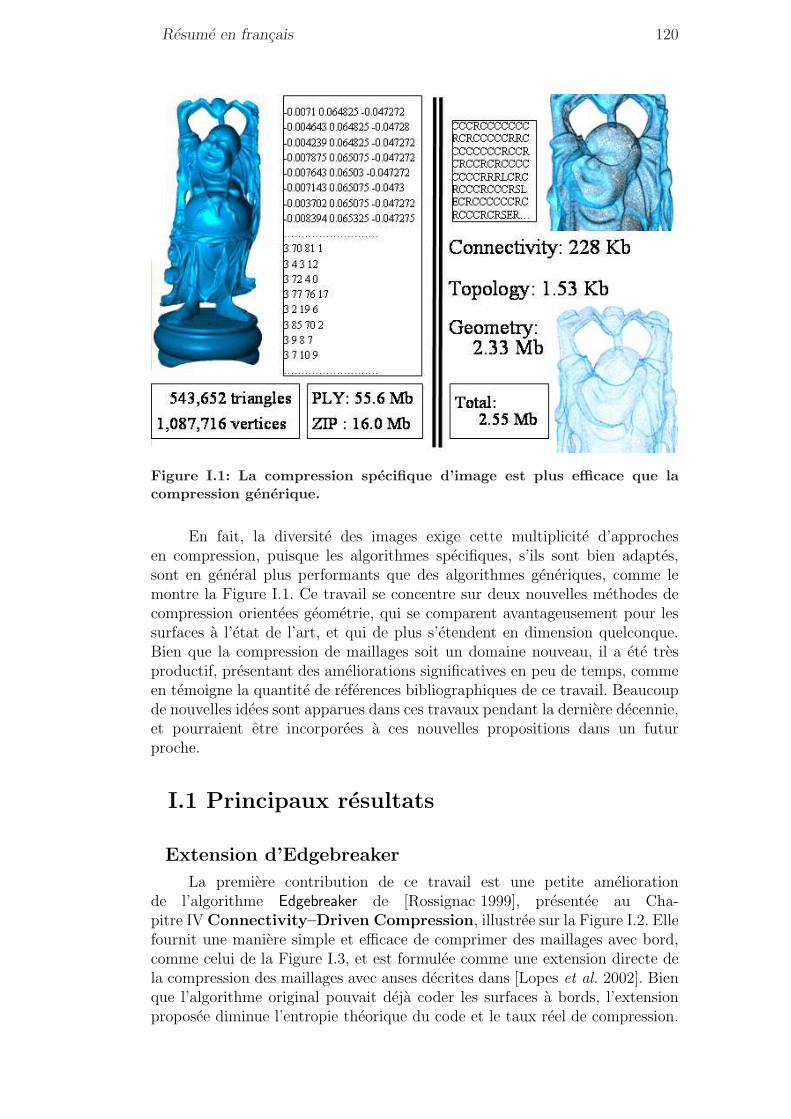
Resume en francais 120

Figure I.1: La compression specifique d’image est plus efficace que lacompression generique.

En fait, la diversite des images exige cette multiplicite d’approchesen compression, puisque les algorithmes specifiques, s’ils sont bien adaptes,sont en general plus performants que des algorithmes generiques, comme lemontre la Figure I.1. Ce travail se concentre sur deux nouvelles methodes decompression orientees geometrie, qui se comparent avantageusement pour lessurfaces a l’etat de l’art, et qui de plus s’etendent en dimension quelconque.Bien que la compression de maillages soit un domaine nouveau, il a ete tresproductif, presentant des ameliorations significatives en peu de temps, commeen temoigne la quantite de references bibliographiques de ce travail. Beaucoupde nouvelles idees sont apparues dans ces travaux pendant la derniere decennie,et pourraient etre incorporees a ces nouvelles propositions dans un futurproche.

I.1 Principaux resultats

Extension d’Edgebreaker

La premiere contribution de ce travail est une petite ameliorationde l’algorithme Edgebreaker de [Rossignac 1999], presentee au Cha-pitre IV Connectivity–Driven Compression, illustree sur la Figure I.2. Ellefournit une maniere simple et efficace de comprimer des maillages avec bord,comme celui de la Figure I.3, et est formulee comme une extension directe dela compression des maillages avec anses decrites dans [Lopes et al. 2002]. Bienque l’algorithme original pouvait deja coder les surfaces a bords, l’extensionproposee diminue l’entropie theorique du code et le taux reel de compression.

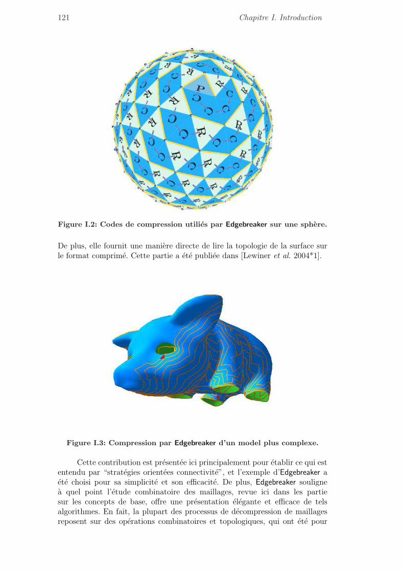
121 Chapitre I. Introduction

Figure I.2: Codes de compression utilies par Edgebreaker sur une sphere.

De plus, elle fournit une maniere directe de lire la topologie de la surface surle format comprime. Cette partie a ete publiee dans [Lewiner et al. 2004*1].

Figure I.3: Compression par Edgebreaker d’un model plus complexe.

Cette contribution est presentee ici principalement pour etablir ce qui estentendu par “strategies orientees connectivite”, et l’exemple d’Edgebreaker aete choisi pour sa simplicite et son efficacite. De plus, Edgebreaker soulignea quel point l’etude combinatoire des maillages, revue ici dans les partiesur les concepts de base, offre une presentation elegante et efficace de telsalgorithmes. En fait, la plupart des processus de decompression de maillagesreposent sur des operations combinatoires et topologiques, qui ont ete pour

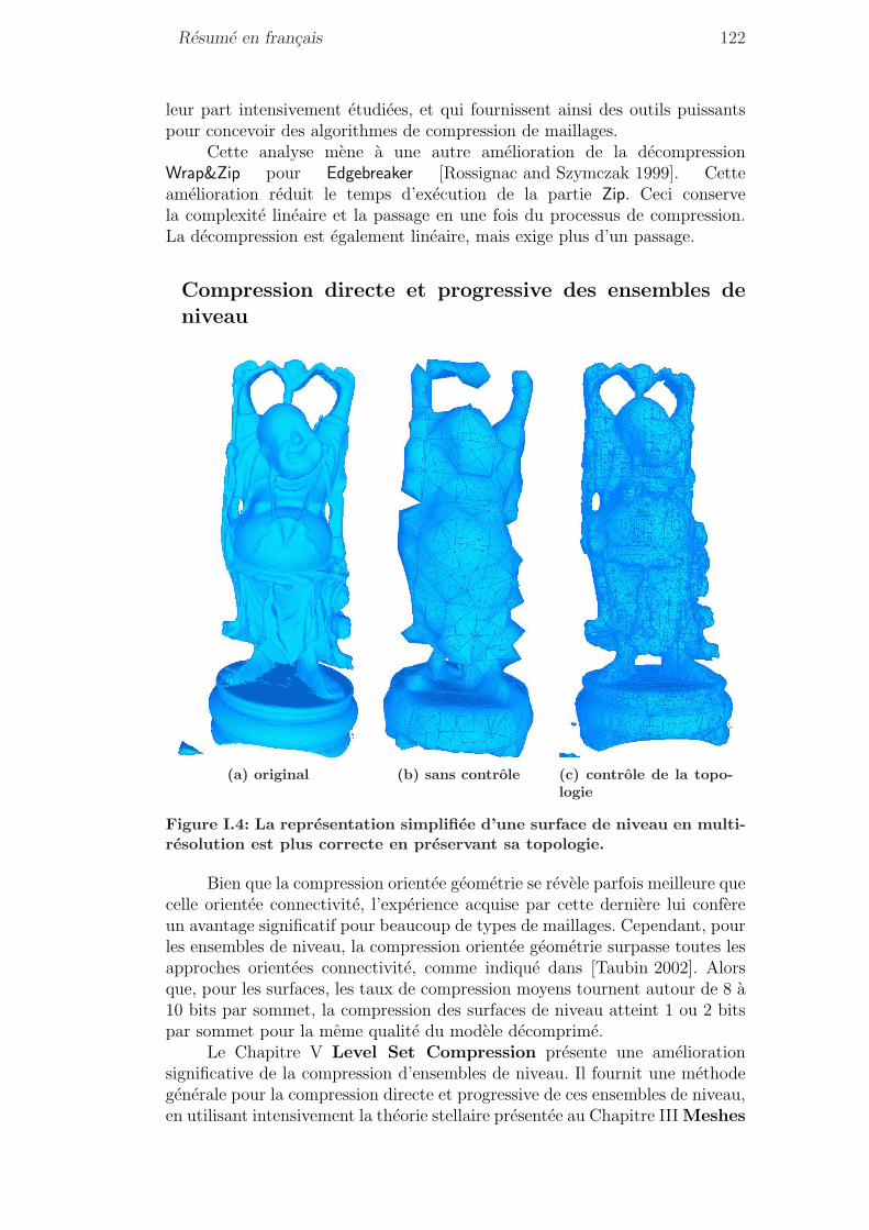
Resume en francais 122

leur part intensivement etudiees, et qui fournissent ainsi des outils puissantspour concevoir des algorithmes de compression de maillages.

Cette analyse mene a une autre amelioration de la decompressionWrap&Zip pour Edgebreaker [Rossignac and Szymczak 1999]. Cetteamelioration reduit le temps d’execution de la partie Zip. Ceci conservela complexite lineaire et la passage en une fois du processus de compression.La decompression est egalement lineaire, mais exige plus d’un passage.

Compression directe et progressive des ensembles deniveau

(a) original (b) sans controle (c) controle de la topo-logie

Figure I.4: La representation simplifiee d’une surface de niveau en multi-resolution est plus correcte en preservant sa topologie.

Bien que la compression orientee geometrie se revele parfois meilleure quecelle orientee connectivite, l’experience acquise par cette derniere lui confereun avantage significatif pour beaucoup de types de maillages. Cependant, pourles ensembles de niveau, la compression orientee geometrie surpasse toutes lesapproches orientees connectivite, comme indique dans [Taubin 2002]. Alorsque, pour les surfaces, les taux de compression moyens tournent autour de 8 a10 bits par sommet, la compression des surfaces de niveau atteint 1 ou 2 bitspar sommet pour la meme qualite du modele decomprime.

Le Chapitre V Level Set Compression presente une ameliorationsignificative de la compression d’ensembles de niveau. Il fournit une methodegenerale pour la compression directe et progressive de ces ensembles de niveau,en utilisant intensivement la theorie stellaire presentee au Chapitre III Meshes

123 Chapitre I. Introduction

Figure I.5: Decompression d’un modele de cheval echantillonne sur unegrille reguliere de taille 2573. Les premieres images correspondent aux raf-finements de la multitriangulation, suivi des raffinements de la geometrie.

and Geometry, ainsi que la structure de [Mello et al. 2003] qui en estdeduite. Cette structure fournit un degre d’adaptabilite tres eleve en sepresentant comme une specification de partition binaires, et permet egalementun controle simple et puissant sur la representation induite en multiresolutiondes ensembles de niveau, comme sur l’exemple de la Figure I.4.

Pour les surfaces de niveau, cette methode offre des rapports entre letaux de compression et la distorsion du modele decomprime au niveau del’etat de l’art, en particulier par comparaison aux methodes basees sur lesoctrees, qui sont des cas particuliers de notre methode comme le montrela Figure I.5. De plus, cette proposition est decrite de la meme maniere pourn’importe quelle dimension, en utilisant seulement les operations stellairessur les aretes du maillage. Son implementation actuelle consomme encorebeaucoup de memoire a l’execution. Les specifications de l’algorithme pourles surfaces ont ete precedemment publiees dans [Lewiner et al. 2004*4], etdans [Lewiner et al. 2004*2, Lewiner et al. 2005*3] pour les courbes.

Compression orientee geometrie generique

Motive par ces resultats, qui renforcent l’idee que les systemes de com-pression orientes geometrie peuvent etre plus efficaces que ceux orientes connec-tivite, nous avons developpe une methode generale de compression directeoriente geometrie, appelee GEncode. Cette methode, sous la forme de l’Al-gorithme 15 : gencode et l’Algorithme 16 : gdecode, supporte n’importe quelcomplexe simplicial ou polytope, de dimension arbitraire et plonge dans unespace ambiant quelconque, comme ceux de la Figure I.6. Pour les surfaces,GEncode offre des taux de compression comparables aux approches orientesconnectivite, bien que la partie de codage geometrique puisse encore etreconsiderablement amelioree. Ces resultats, presentes au Chapitre VI GEn-code, ont ete precedemment publies dans [Lewiner et al. 2005*1].

Le cœur de cette methode comporte un critere geometrique pour coder laconnectivite du maillage. Ce critere est une fonction a valeurs reelles arbitrairequi doit caracteriser la geometrie d’une cellule du maillage a coder. Plus lecritere correspond au maillage, meilleur est le taux de compression et le tempsd’execution. Pour illustrer ce concept, nous avons derive un critere geometriquedu a partir du rayon de la sphere circonscrite a une cellule. Ce critere s’adapte

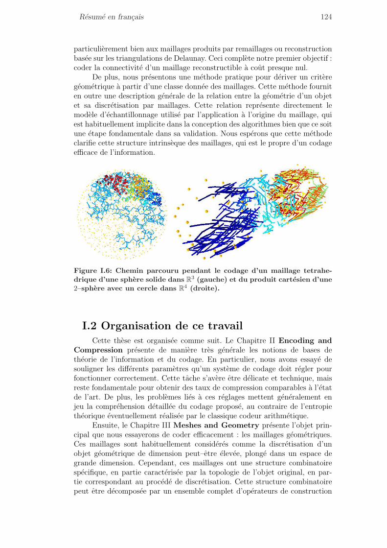
Resume en francais 124

particulierement bien aux maillages produits par remaillages ou reconstructionbasee sur les triangulations de Delaunay. Ceci complete notre premier objectif :coder la connectivite d’un maillage reconstructible a cout presque nul.

De plus, nous presentons une methode pratique pour deriver un criteregeometrique a partir d’une classe donnee des maillages. Cette methode fourniten outre une description generale de la relation entre la geometrie d’un objetet sa discretisation par maillages. Cette relation represente directement lemodele d’echantillonnage utilise par l’application a l’origine du maillage, quiest habituellement implicite dans la conception des algorithmes bien que ce soitune etape fondamentale dans sa validation. Nous esperons que cette methodeclarifie cette structure intrinseque des maillages, qui est le propre d’un codageefficace de l’information.

Figure I.6: Chemin parcouru pendant le codage d’un maillage tetrahe-drique d’une sphere solide dans R3 (gauche) et du produit cartesien d’une2–sphere avec un cercle dans R4 (droite).

I.2 Organisation de ce travailCette these est organisee comme suit. Le Chapitre II Encoding and

Compression presente de maniere tres generale les notions de bases detheorie de l’information et du codage. En particulier, nous avons essaye desouligner les differents parametres qu’un systeme de codage doit regler pourfonctionner correctement. Cette tache s’avere etre delicate et technique, maisreste fondamentale pour obtenir des taux de compression comparables a l’etatde l’art. De plus, les problemes lies a ces reglages mettent generalement enjeu la comprehension detaillee du codage propose, au contraire de l’entropietheorique eventuellement realisee par le classique codeur arithmetique.

Ensuite, le Chapitre III Meshes and Geometry presente l’objet prin-cipal que nous essayerons de coder efficacement : les maillages geometriques.Ces maillages sont habituellement consideres comme la discretisation d’unobjet geometrique de dimension peut–etre elevee, plonge dans un espace degrande dimension. Cependant, ces maillages ont une structure combinatoirespecifique, en partie caracterisee par la topologie de l’objet original, en par-tie correspondant au procede de discretisation. Cette structure combinatoirepeut etre decomposee par un ensemble complet d’operateurs de construction

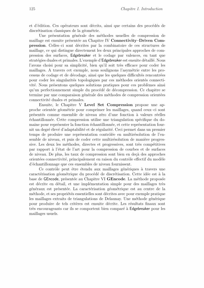
125 Chapitre I. Introduction

et d’edition. Ces operateurs sont decrits, ainsi que certains des procedes dediscretisation classiques de la geometrie.

Une presentation generale des methodes usuelles de compression demaillage est ensuite presentee au Chapitre IV Connectivity–Driven Com-pression. Celles–ci sont decrites par la combinatoire de ces structures demaillage, ce qui distingue directement les deux principales approches de com-pression des surfaces, Edgebreaker et le codage par valences, en tant questrategies duales et primales. L’exemple d’Edgebreaker est ensuite detaille. Nousl’avons choisi pour sa simplicite, bien qu’il soit tres efficace pour coder lesmaillages. A travers cet exemple, nous soulignons l’asymetrie entre les pro-cessus de codage et de decodage, ainsi que les quelques difficultes rencontreespour coder les singularites topologiques par ces methodes orientes connecti-vite. Nous presentons quelques solutions pratiques pour ces problemes ainsiqu’un perfectionnement simple du procede de decompression. Ce chapitre setermine par une comparaison generale des methodes de compression orienteesconnectivite duales et primales.

Ensuite, le Chapitre V Level Set Compression propose une ap-proche orientee geometrie pour comprimer les maillages, quand ceux–ci sontpresentes comme ensemble de niveau zero d’une fonction a valeurs reellesechantillonnee. Cette compression utilise une triangulation specifique du do-maine pour representer la fonction echantillonnee, et cette representation four-nit un degre eleve d’adaptabilite et de regularite. Ceci permet dans un premiertemps de produire une representation controlee en multiresolution de l’en-semble de niveau, et puis de coder cette multiresolution de maniere progres-sive. Les deux les methodes, directes et progressives, sont tres competitivespar rapport a l’etat de l’art pour la compression de courbes et de surfacesde niveau. De plus, les taux de compression sont bien en deca des approchesorientees connectivite, principalement en raison du controle effectif du modeled’echantillonnage que ces ensembles de niveau fournissent.

Ce controle peut etre etendu aux maillages generiques a travers unecaracterisation geometrique du procede de discretisation. Cette idee est a labase de GEncode, presentee au Chapitre VI GEncode. La methode proposeeest decrite en detail, et une implementation simple pour des maillages tresgeneraux est presentee. La caracterisation geometrique est au centre de lamethode, et ses proprietes essentielles sont decrites avec pour exemple pratiqueles maillages extraits de triangulations de Delaunay. Une methode generiquepour produire de tels criteres est ensuite decrite. Les resultats finaux sonttres encourageants car ils se comportent bien compare a Edgebreaker pour lesmaillages usuels.

II Codage et Compression

Ce travail vise a definir de nouvelles methodes pour comprimer les objetsgeometriques. Nous voudrions d’abord presenter brievement ce que entendonspar compression, en particulier la relation entre l’outil abstrait de la theorie del’information [Nyquist 1928, Hartley 1928, Shannon 1948], l’entropie asymp-totique des codes [Shannon 1948, Huffman 1952, Tutte 1998] et les perfor-mances pratiques des algorithmes de codage [Huffman 1952, Rissanen 1976,Lempel and Ziv 1977, Moffat et al. 1995]. Nous nous concentrerons ensuite surle codeur arithmetique [Rissanen 1976, Moffat et al. 1995], car c’est celui quenous emploierons dans la pratique. Ce codeur peut etre ameliore par la priseen compte des informations, deterministes ou statistiques, de l’objet a co-der, ce qui se traduit techniquement par un passage de l’entropie de Shan-non [Shannon 1948] a la complexite de Kolmogorov [Li and Vitanyi 1997]. En-fin, nous decrirons comment ce codage fait partie des schemas de compression.Des references generales sur la compression de donnees peuvent etre trouveesdans [Salomon 2000].

II.1 Representation de l’Information

Source et codes. Le codage est un procede simple de traduction quiconvertit des symboles d’un ensemble, appele la source, vers un autre, appelel’ensemble des codes. La conversion doit aussi pouvoir etre appliquee dansl’autre sens, afin de recuperer la sequence originale de symboles, appelee lemessage. Le but est de representer n’importe quel message de la source plusefficacement, typiquement pour s’adapter a un canal de transmission specifique.Ce codage peut chercher a reduire la taille du message [Salomon 2000],par exemple pour des applications de compression, ou au contraire pouraugmenter sa redondance, afin de pouvoir detecter d’eventuelles erreurs detransmission [Hamming 1950].

Enumeration. Un exemple simple de codeur enumererait tous les messagespossibles, en les numerotant de 1 a n pendant l’enumeration. Le codeurassignerait alors simplement un code pour chaque message. Dans la pratique,le nombre de possibilites est enorme et difficile a enumerer, et il est difficilede recuperer le message original a partir de son index sans avoir a enumerertous les messages possibles. Ceci peut quand meme fonctionner pour des casspecifiques [Castelli and Devillers 2004]. Ces codeurs enumeratifs donnent unereference pour comparer l’execution des codeurs. Cependant, dans les caspratiques, nous voudrions que le codage soit plus efficace pour les messages les

Resume en francais 128

plus frequents, meme si la performance se degrade pour les moins frequents.Cette reference ne sera alors pas notre objectif principal.

Performances des codeurs. Deux codages differents de la meme sourceproduisent en general deux messages codes de tailles differentes. Si nous avonsl’intention de reduire la taille du message, nous prefererons le codeur quiproduit du plus petit message. Sur un exemple specifique, ceci peut etredirectement mesure. D’ailleurs, pour le codeur enumeratif, l’execution estsimplement le logarithme du nombre d’elements, puisqu’un nombre n peutetre represente par des chiffres de log pnq. Cependant, cette performance estdifficile a mesurer pour tous les messages possibles d’une application donnee.[Nyquist 1928], [Hartley 1928] et [Shannon 1948] ont presente un outil generalpour mesurer la performance asymptotique et theoretique d’un code, appelel’entropie.

II.3 CompressionLe codage est seulement une partie d’un schema de compression. En

fait, un schema de compression se compose de diverses etapes de conversions,depuis les donnees originales vers une representation symbolique, puis de cetterepresentation a la specification des sources, de ces sources a un message code,de ce message code en protocole de transmission, qui necessite un re–codagepour la detection des erreurs, et enfin les parties symetriques du cote recepteur.

Ce processus entier peut etre concu partie par partie, ou comme untout. Par exemple, certains schemas de compression astucieux incorporentdeja la detection d’erreurs, en utilisant la redondance des donnees originalesqui restent apres le codage. Quelques schemas de compression avec pertes ouprogressifs effectuent le codage directement a partir de la representation etincorporent la specification des sources.

Ces aspects optimisent la compression pour des applications specifiques.Cependant, une application generique exige en general une conception separeedes parties d’un schema de compression. Dans ce contexte, le codagearithmetique s’avere etre un outil tres flexible pour ajuster le taux de com-pression final, i.e. le rapport entre la taille finale et originale des donnees.Selon l’application, ce rapport de compression doit etre reduit pour optimisercertaines caracteristiques de ces applications, donnant lieu a differents com-promis. Nous allons maintenant detailler trois compromis generiques.

(a) Compaction

La compaction se rapporte aux structures de donnees compactes,egalement appelees succinctes. Ces structures cherchent a reduire la taille dela memoire utilisee pendant l’execution d’une application, tout en necessitantpeu de temps d’execution supplementaire. Ce compromis entre la memoireutilisee et le temps d’execution doit en plus permettre un acces aleatoirea la structure de donnees compacte. Par exemple pour des structures dedonnees de maillage, ce compromis peut etre simplement une representationelegante des donnees sans codage specifique, comme [Rossignac et al. 2001,

129 Chapitre II. Codage et Compression

Lage et al. 2005*1, Lage et al. 2005]. Il peut egalement impliquer un schema decodage simple qui soit rapide a interpreter, comme [Houston et al. 2005], ou en-core un melange precis d’un codage tres efficace avec une structure de donneesde plus haut niveau, comme [Castelli et al. 2005*1, Castelli et al. 2005*2].

(b) Compression Directe

La signification la plus utilisee de la compression se rapporte ala compression de fichiers ou a la compression d’information echangee.La plupart des algorithmes generiques usuels sont basees sur l’algo-rithme LZH (ZIP) de [Lempel and Ziv 1977], hormis quelques algorithmesspecifiques de compression d’image et de video tels que JPEG [Wallace 1991,Christopoulos et al. 2000] et MPEG [le Gall 1991, Pereira and Ebrahimi 2002].Dans ce cas, le but est d’optimiser le compromis entre le taux de compression etle temps necessaire pour comprimer : la methode d’enumeration est habituel-lement trop lente, alors qu’un codage simple de la representation de donneespeut etre en general ameliore sans presque augmenter le temps d’execution. Lecompromis peut egalement tenir compte de la quantite de memoire necessairepour comprimer ou decomprimer le message. Dans ce cas, le processus esthabituellement execute hors noyau, comme [Isenburg and Gumhold 2003].

(c) Compression Progressive

La compression peut egalement mener a une perte d’information endecomprimant. Ceci peut etre utile soit quand la partie perdue n’est passignificative, soit quand elle peut etre recuperee par une autre etape decompression. Dans ce deuxieme sens, la compression avec pertes produira desobjets a de divers niveaux de detail, i.e. en multiresolution. Chaque resolutionpeut etre comprimee separement par difference avec la precedente. Une variantede ce schema ne distingue pas un niveau de detail du suivant, envoyant unniveau brut par compression directe, puis le raffinant par une sequence demodifications locales. Dans ce contexte, le but est d’optimiser le compromisentre le taux de compression et la distorsion du modele decomprime. Pourles modeles geometriques, la deformation est habituellement mesuree par ladistance geometrique entre le modele decode et l’original.

III Maillages et Geometrie

Les objets geometriques sont habituellement representes par desmaillages. Particulierement pour les surfaces dans l’espace, les triangulationsont eu l’avantage de representer beaucoup de pixels sur l’ecran par un seul tri-angle. Bien que la taille croissante des maillages usuels ait reduit cet avantage,le materiel graphique et les algorithmes sont optimises pour ces representationset les maillages sont encore predominants sur les modeles par ensemble depoint. D’ailleurs, plusieurs parties des traitements sans maillages necessitentencore la generation de maillages locaux, qui devient tres couteuse en dimen-sions elevees. Enfin, les maillages decrivent d’une facon unique et explicite lesupport de l’objet geometrique, par interpolation morceau a morceau ou parparametrisation locale telle que les splines ou les NURBS.

A un objet reel correspondent plusieurs maillages. Ces maillagesrepresentent la meme geometrie et la meme topologie, et different donc parleur connectivite. La maniere dont ces objets sont echantillonnes depend del’application, variant depuis la visualisation jusqu’aux methodes d’anima-tion et d’element fini. Ces variations rendent difficile une definition de qua-lite geometrique d’un maillage independante de l’application, meme avec unedefinition commune pour la connectivite.

Ce chapitre detaille la partie combinatoire, presentant la definition etles proprietes des maillages dans la Section III.1 Simplicial Complexes and Po-lytopes, et un ensemble complet d’operations sur la connectivite dans la Sec-tion III.2 Combinatorial Operators. Enfin, la Section III.3 Geometry and Discreti-sation donne quelques exemples classiques des interactions entre la geometrieet les maillages.

Dans ce travail, nous n’employons pas une structure de donneesspecifique pour les maillages. Nous considererons les operations decritesdans ce chapitre comme les elements de base d’une structure de donneesgenerique. Pour approfondir, les structures de donnees classiques pourdes surfaces sont winged–edge [Baumgart 1972], split–edge [Eastman 1982],quad–edge [Guibas and Stolfi 1985], half–edge [Mantyla 1988] etcorner–table [Rossignac et al. 2001, Lage et al. 2005]. Pour les maillages non–varietes, nous mentionnerions radial–edge [Weiler 1985] et [de Floriani and Hui 2003].D’autres references sur les definitions suivantes peuvent etre trouveesdans [Munkres 1984, Boissonnat and Yvinec 1998, Hatcher 2002].

IV Compression Orientee Connectivite

Ce travail vise a comprimer les objets geometriques representes par desmaillages. Puisqu’il n’y a pas encore de relation forte entre la geometrieet la connectivite pour les maillages usuels des applications graphiques, lesalgorithmes de compression dedies considerent que l’information communepeut etre deduite soit de la connectivite soit de la geometrie. La premiereoption suppose que l’etoile d’un simplexe a une geometrie simple, qui peut etrecorrectement approchee par des methodes simples telles que l’interpolationlineaire. Puis, la geometrie peut etre efficacement codee par un parcours dela connectivite du maillage, menant aux schemas de compression orienteeconnectivite. La deuxieme option predit la connectivite a partir de la geometrie,et sera designee comme schemas de compression orientes geometrie. Dans cecas, la connectivite est en general mieux comprimee, mais ces schemas ontbesoin d’un codage efficace de la geometrie.

Dans ce chapitre, nous nous concentrerons sur la partie connectivite de lacompression, afin de clarifier la position de la compression orientee geometriedes prochains chapitres. Ces methodes orientees connectivite se sont telle-ment ameliorees dans la derniere decennie que le taux de compression pourla connectivite des surfaces usuelles tourne autour de 2/3 bits par sommet.Nous donnerons un cadre general pour manipuler les elements critiques de laconnectivite : les singularites topologiques. Ces singularites des surfaces sontbien explicitees par les operateurs de poignee de la Section III.2(b) HandleOperators. Nous nous concentrerons ensuite sur l’algorithme Edgebreaker, etpresenterons deux nouvelles ameliorations : la manipulation des bords, commeconsequence de cette formalisation des singularites, et une petite ameliorationde l’algorithme de decompression. Nous conclurons ce chapitre avec les taux decompression d’Edgebreaker sur les modeles habituels avec nos ameliorations, etnous detaillerons les specificites des schemas de compression oriente connecti-vite. Le but de ce chapitre est d’enoncer ce que signifie la compression orienteeconnectivite, avec l’exemple detaille d’Edgebreaker, pour voir quand ces algo-rithmes sont bien adaptes.

PrincipesLes schemas de compression orientes connectivite se fondent sur un

parcours du maillage afin de visiter chaque sommet une fois, et l’identi-fier au cours des visites suivantes. De cette facon, la geometrie du som-met doit etre transmise seulement une fois, et le parcours code la connec-tivite du maillage. Ce cadre de general convient particulierement bienpour les polytopes qui sont des varietes. La plupart des techniques exis-

Resume en francais 134

tantes de compression sont consacrees aux surfaces, et nous nous concen-trerons sur ces algorithmes. D’autres prolongements aux cas des non–varietes sont decrits dans [Gueziec et al. 1998], alors que les prolongementssimples des schemas les plus communs existent pour les modeles solides,comme [Szymczak and Rossignac 2000, Isenburg and Alliez 2002].

La compression orientee connectivite a commence par des problemesd’optimisation de memoire cache dans les cartes graphiques : la maniere detransmettre des maillages triangulaires a partir de la memoire centrale versla carte graphique est (encore aujourd’hui) d’envoyer les trois sommets dutriangle, representes par leurs trois coordonnees en representation en virguleflottante. Chaque triangle est alors code avec 96 bits ! [Deering 1995] a proposede representer ces maillages triangulaires par les bandes generalisees, afin departager un ou deux sommets avec le dernier triangle transmis, reduisant aumoins de moitie la memoire requise precedemment. Ce mecanisme emploieegalement un petit schema de prevision pour optimiser le cache.

Puis, ces bandes ont ete generalisees par une approche de chi-rurgie topologique dans [Taubin and Rossignac 1998, Taubin et al. 1998].Ces travaux ont presente le cadre le plus general pour la com-pression orientee connectivite, et ont ete efficacement derives dansEdgebreaker [Rossignac 1999], et de maniere plus flexible dans le co-dage par valence de [Touma and Gotsman 1998, Alliez and Desbrun 2001].L’Edgebreaker a ete etendu pour manipuler une plus grande categorie desurfaces dans [Lopes et al. 2002, Lewiner et al. 2004], alors que le codage parvalence a ete regle en utilisant la geometrie dans [Alliez and Desbrun 2001],et la geometrie discrete dans [Kalberer et al. 2005]. En outre, le par-cours du codage par valence peut eviter les codes d’echappement en uti-lisant [Castelli and Devillers 2004].

Avec ces ameliorations, la connectivite des modeles habituelspeut etre comprimee avec quelques bits par sommet. La geometrieest devenue la partie la plus chere, qui peut etre reduite en utilisantprediction [Touma and Gotsman 1998, Cohen–Or et al. 2001] et quantifi-cation de haute qualite [Sorkine et al. 2003, Gumhold and Amjoun 2004].Cependant, nous ne nous concentrerons pas ici sur la compression de lageometrie.

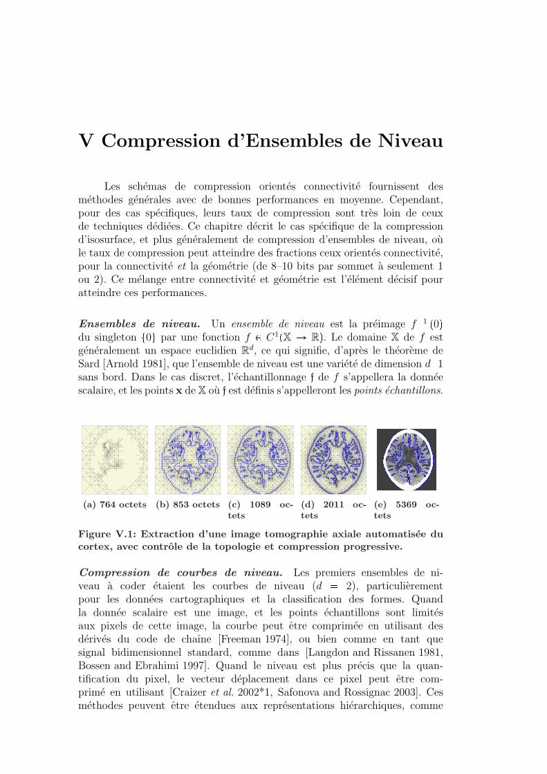
V Compression d’Ensembles de Niveau

Les schemas de compression orientes connectivite fournissent desmethodes generales avec de bonnes performances en moyenne. Cependant,pour des cas specifiques, leurs taux de compression sont tres loin de ceuxde techniques dediees. Ce chapitre decrit le cas specifique de la compressiond’isosurface, et plus generalement de compression d’ensembles de niveau, oule taux de compression peut atteindre des fractions ceux orientes connectivite,pour la connectivite et la geometrie (de 8–10 bits par sommet a seulement 1ou 2). Ce melange entre connectivite et geometrie est l’element decisif pouratteindre ces performances.

Ensembles de niveau. Un ensemble de niveau est la preimage f�1 p0qdu singleton t0u par une fonction f P C1pX Ñ Rq. Le domaine X de f estgeneralement un espace euclidien Rd, ce qui signifie, d’apres le theoreme deSard [Arnold 1981], que l’ensemble de niveau est une variete de dimension d�1sans bord. Dans le cas discret, l’echantillonnage f de f s’appellera la donneescalaire, et les points x de X ou f est definis s’appelleront les points echantillons.

(a) 764 octets (b) 853 octets (c) 1089 oc-tets

(d) 2011 oc-tets

(e) 5369 oc-tets

Figure V.1: Extraction d’une image tomographie axiale automatisee ducortex, avec controle de la topologie et compression progressive.

Compression de courbes de niveau. Les premiers ensembles de ni-veau a coder etaient les courbes de niveau (d � 2), particulierementpour les donnees cartographiques et la classification des formes. Quandla donnee scalaire est une image, et les points echantillons sont limitesaux pixels de cette image, la courbe peut etre comprimee en utilisant desderives du code de chaıne [Freeman 1974], ou bien comme en tant quesignal bidimensionnel standard, comme dans [Langdon and Rissanen 1981,Bossen and Ebrahimi 1997]. Quand le niveau est plus precis que la quan-tification du pixel, le vecteur deplacement dans ce pixel peut etre com-prime en utilisant [Craizer et al. 2002*1, Safonova and Rossignac 2003]. Cesmethodes peuvent etre etendues aux representations hierarchiques, comme

Resume en francais 136

dans [Lopes et al. 2002*1], et puis aux schemas progressifs de compres-sion, comme cela est effectue dans [le Buhan and Ebrahimi 1997] par larepresentation hierarchique induite par une multiresolution de l’image.

Applications des Isosurfaces. Les isosurfaces (d � 3) sont lar-gement repandues dans beaucoup de domaines, depuis les imagesmedicales [Lorensen and Cline 1987] jusqu’a l’infographie [Parker et al. 1998]et la reconstruction de surface [Davis et al. 2002], en passant par lemodelage geophysique [Tavares et al. 2003] et la visualisation scienti-fique [Bajaj et al. 1998]. Par exemple, les techniques d’imagerie medicaletelles que la tomographie axiale automatisee et la resonance magnetiquemesurent des quantites physiques echantillonnees sur une grille semi–reguliere tridimensionnelle. En outre pour les simulations scientifiques,des equations aux derivees partielles sont generalement resolues en utili-sant des methodes d’ensembles de niveau, comme ceux de [Sethian 1999],qui resultent egalement en une fonctionne echantillonnee sur une grille tri-dimensionnelle. Cette variete d’applications a egalement genere un largeattirail de technique pour manipuler les isosurfaces [Bloomenthal et al. 1997].Ces isosurfaces peuvent etre structurees en maillages par la methodeusuelle de Marching Cubes de [Lorensen and Cline 1987] et ses exten-sions [Nielson and Hamann 1991, Montani et al. 1994, Lewiner et al. 2003*3],par le contour dual de [Ju et al. 2002] et les methodes simplicialesde [Velho 1996, Treece et al. 1999].

Compression d’Isosurfaces. Dans la plupart des applications des iso-surfaces, le resultat visuel est seulement une surface extraite a partir desdonnees scalaires par interpolation de f. Par exemple, le cortex correspondseulement a une scintillation specifique de rayons X a l’interieur de l’imagede la tete entiere. Dans ce cas, regarder seulement ce cortex permet de je-ter la majeure partie des donnees scalaires, puisque le cortex reconstruit estcontenu seulement dans une partie limitee de la tete. Ceci motive des tech-niques specifiques pour comprimer les isosurfaces en codant seulement la partieessentielle des donnees scalaires. De plus, ces techniques montrent de meilleuresperformances que des methodes generiques de compression de maillage. Bienque [Saupe and Kuska 2002] et [Yang and Wu 2002] aient deja developpe desmethodes de compression specifiques pour les isosurfaces, leur codage exten-sif base sur les configurations de Marching Cube ont ete rapidement depassespar la compression JBIG des donnees scalaires, et puis par [Taubin 2002] quia etendu ce codage arithmetique avec un contexte dans chacune des trois di-mensions des donnees scalaires. Puis, [Boada and Navazo 2001] ont propose decoder seulement la partie specifique des donnees scalaires contenant l’isosur-face, d’une facon progressive basee sur une decomposition en octree des donneesscalaires. Une petite amelioration de ce travail, proposee dans [Lee et al. 2003],acheve la compression avec un codage final de la geometrie au niveau du detaille plus fin.

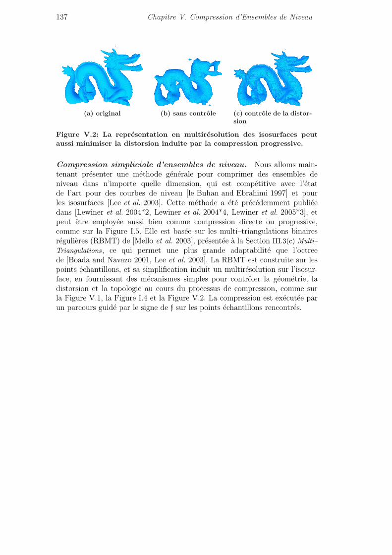
137 Chapitre V. Compression d’Ensembles de Niveau

(a) original (b) sans controle (c) controle de la distor-sion

Figure V.2: La representation en multiresolution des isosurfaces peutaussi minimiser la distorsion induite par la compression progressive.

Compression simpliciale d’ensembles de niveau. Nous alloms main-tenant presenter une methode generale pour comprimer des ensembles deniveau dans n’importe quelle dimension, qui est competitive avec l’etatde l’art pour des courbes de niveau [le Buhan and Ebrahimi 1997] et pourles isosurfaces [Lee et al. 2003]. Cette methode a ete precedemment publieedans [Lewiner et al. 2004*2, Lewiner et al. 2004*4, Lewiner et al. 2005*3], etpeut etre employee aussi bien comme compression directe ou progressive,comme sur la Figure I.5. Elle est basee sur les multi–triangulations binairesregulieres (RBMT) de [Mello et al. 2003], presentee a la Section III.3(c) Multi–Triangulations, ce qui permet une plus grande adaptabilite que l’octreede [Boada and Navazo 2001, Lee et al. 2003]. La RBMT est construite sur lespoints echantillons, et sa simplification induit un multiresolution sur l’isosur-face, en fournissant des mecanismes simples pour controler la geometrie, ladistorsion et la topologie au cours du processus de compression, comme surla Figure V.1, la Figure I.4 et la Figure V.2. La compression est executee parun parcours guide par le signe de f sur les points echantillons rencontres.

VI GEncode

Parmi les algorithmes de compression de maillages, differents schemascompriment mieux certaines categories de modele. En particulier, nous avonsvu dans le dernier chapitre que les approches orientees geometrie ont desperformances exceptionnelles pour les isosurfaces. Il serait attendu de cesalgorithmes qu’ils codent egalement bien les maillages reconstruits a partirde la geometrie, ou optimises par remaillage geometrique. Ces maillagesadaptes a la geometrie sont habituellement chers a calculer, soit dans le casde la reconstruction, comme par exemple avec [Amenta et al. 2001], soit parremaillage comme dans [Alliez et al. 2003, Alliez et al. 2003]. De plus, leurgeometrie est parfois connue independamment de leur connectivite, telle quepour les resultats de scans, et le seul codage de leur connectivite peut etre utiledans ce contexte.

Nous allons maintenant presenter GEncode, precedemment publiedans [Lewiner et al. 2005*1], qui est un schema de compression directe demaillages et qui comprime la connectivite de ces maillages geometriques a coutpresque zero. Cet algorithme est tres general, et traite de complexes simpliciauxde dimension arbitraire plonges dans un espace ambiant arbitraire, meme si lecomplexe n’est ni pur, ni variete et ni orientable. Les resultats de compressionpour des surfaces sont concurrentiels avec des schemas de compression orientesconnectivite existants.

VI.1 Objectifs

(a) Adaptation aux maillages geometriques

Nous nous concentrerons sur les maillages geometriques, c’est a dire lesmaillages dont la connectivite est deduite de leur geometrie, comme les re-constructions de scans ou les modeles remailles, ainsi que sur les maillages dedimension elevee ou avec une topologie complexe. Dans ces cas, les approchesde compression orientees connectivite devraient etre moins efficaces sur le co-dage de la connectivite. D’une part, la connectivite des maillages geometriquespeut etre partiellement deduite de la geometrie, et la connectivite n’a ainsi pasmeme besoin d’etre codee. D’autre part, les codes de connectivite deviennentexponentiellement complexes avec la dimension, alors que les codes de connecti-vite orientes geometrie manipulent tres simplement des topologies complexes,comme nous allons le detailler maintenant. Ces particularites ont ete dejaenoncees dans [Gandoin and Devillers 2002], qui etait le premier algorithmede compression progressif et oriente geometrie.

Resume en francais 140

De plus, nous voudrions que notre algorithme soit previsible et flexible.Plus precisement, puisque cette methode est adaptee a une categorie specifiquedes maillages, comme la compression orientee connectivite ou la compressiond’ensembles de niveau etait adaptees a d’autres categories, nous voudrionssavoir par un test simple si notre algorithme sera performant avant la com-pression par elle-meme. En outre, selon le type de maillage, i.e. les maillagesde conception assistee par ordinateur, les supports des methodes d’elementsfinis, les maillages se scans ou remailles. . . , l’algorithme devrait employer uncritere geometrique different pour etre adapte aux caracteristiques propres ala generation de ces maillages. Nous nous concentrerons sur le critere du BallPivoting puisqu’il est facile a comprendre et a implementer en n’importe quelledimension, bien que notre algorithme fonctionne avec n’importe quel criteregeometrique.

Dans le cas des scans, l’algorithme de reconstruction calcule la connec-tivite de la surface seulement a partir de la geometrie de ses sommets. Parconsequent, une approche orientee geometrie employant le meme algorithmede reconstruction ne devrait gaspiller aucun bit dans la connectivite. Le schemapropose atteint ce but, en codant un maillage base sur un critere geometriquelocal.

(b) Cout Nul pour des Maillages Reconstructibles

Vue d’ensemble de la compression. Le schema de codage proposefonctionne de facon similaire aux algorithmes de reconstruction, bien qu’ilcode en continu les differences entre le maillage original et reconstruit.Il code d’abord la geometrie de chaque sommet, dans n’importe quel es-pace ambiant, en utilisant un codage simple d’octree, qui est une synthesede [Gandoin and Devillers 2002] et [Botsch et al. 2002], comme par exemplesur la Figure I.6. L’algorithme code alors la connectivite d’une n–variete enconquerrant la triangulation a partir d’une cellule initiale, attachant a chaqueetape une n–cellule τn�1 � twju a une (n�1)–cellule du bord τn�1.

Codage par deviation. La difference entre le maillage original et lemaillage resultant d’un procede de reconstruction est que w n’est pas toujourscelui qui minimise le critere geometrique G pτn�1, wq du procede de reconstruc-tion. Cette difference est codee par la position de w dans une liste de candidats.Ces candidats sont choisis a partir d’une limite de quantisation sur G pτn�1, wq.Entropie pour les maillages reconstructibles. Pour reduire au mini-mum l’entropie (au sens de la Section II.1(b) Information Theory), cette listeest ordonnee par le critere geometrique. Par consequent, quand le maillage estreconstructible par le critere geometrique donne, le candidat est toujours lepremier et la quantification produit de seulement une classe. Par consequent,les symboles a coder sont tous identiques dans ce cas, et le message a uneentropie nulle, ce qui etait notre objectif.

141 Chapitre VI. GEncode

Maillages generaux. Quand le critere geometrique correspond a laconstruction du maillage, l’entropie est presque nulle. Autrement, les maillagesgeneraux exigent de trouver un critere geometrique adapte pour coder ladeviation entre la reconstruction et le modele original comme decrit ci–dessus. D’un point de vue geometrique, les maillages usuels ne sont pas aussigeneriques, puisque leurs simplexes sont relativement bien formes et relientprincipalement des sommets voisins. Leur geometrie locale est donc relative-ment simple, ce qui motive de chercher des criteres geometriques parametriquespour s’adapter a la geometrie de ces maillages.

Extensions. Du point de vue de la connectivite, l’algorithme peut etre fa-cilement etendu. L’algorithme generique n’a pas besoin d’etre modifie en pas-sant en dimension ou en codimension superieures. Pour les maillages non–simpliciaux, l’operation d’attachement peut exiger plus d’un sommet. Le pre-mier est code comme precedemment, et les autres sont choisis afin d’appartenirau meme hyperplan, et dans l’ordre croissant de leur critere geometrique. Pourdes n–maillages non–varietes, beaucoup de n–cellules peuvent etre attacheesa la meme (n�1)–cellule de la frontiere active. Pour les maillages non–purs,le codage est effectue successivement pour chaque dimension, completant pro-gressivement la structure de dimension la plus elevee avec celles de dimensionsinferieures.

VII Conclusions et Travaux Futurs

Ce travail a propose deux nouvelles methodes de compression orienteesgeometrie pour des maillages en dimension arbitraire, tout en montrant debonnes performances compare a l’etat de l’art pour les basses dimensions.

La premiere methode est limitee aux ensembles de niveau, mais fournitdeux codages direct et progressif avec un large controle sur la progression dansle dernier cas.

Le maillage peut etre raffine en subdivisant son espace ambiant oubien en transmettant des valeurs plus precises pour la fonction implicitedefinissant l’ensemble de niveau. Ces deux methodes sont complementaireset concurrentes, et une suite possible de ce travail pourrait etudier commentoptimiser leur interaction en pratique.

De plus, un modele general du maillage peut etre a priori traduit parune subdivision specifique de l’espace ambiant. Par exemple pour les imagesmedicales d’un certain organe, il est possible de travailler sur l’image d’unesubdivision reguliere d’un cube dans un espace plus dense pres du modelede cet organe. De nouveau, le gain d’une telle methode pourrait motiver uneetude plus detaillee. Cependant, le codage de l’ensemble de niveau peut alorsrepresenter plus qu’un format compact d’image, puisqu’il decrit une certainedeviation du vrai niveau par rapport au modele.

La deuxieme methode est une strategie de codage direct tres generale quipeut traiter n’importe quelle maillage de n’importe quelle topologie, dimensionet dans n’importe quel espace ambiant. GEncode visait a l’origine a coder laconnectivite de maillage des maillages previsible a cout presque nul. Ce butest atteint realise si la regle de prevision est connue.

Cette strategie peut etre amelioree de beaucoup de manieres. D’abord,le codage separe de la geometrie resulte encore en un taux de compressionplus eleve que les approches orientees connectivite. D’un cote, la techniquede codage de la geometrie que nous avons employee est l’une de premiere dugenre, et elle peut surement etre amelioree independamment du reste. D’unautre cote, le melange du codage de la geometrie et de connectivite menehabituellement a des programmes plus efficaces, comme nous l’avons vu pourla compression des ensembles de niveau. Par exemple, ce melange a pu etremis en application par une alternance entre le codage de la connectivite et dela geometrie, le resultat de l’un guidant l’autre.

Nous avons ensuite propose une methode tres generale pour adapterle critere geometrique a une classe specifique de maillages. Elle peut etredirectement employee pour ameliorer les taux de compression pour une laclasse de modeles etudies, mais la recherche du meilleur critere genere de faitbeaucoup plus d’informations. En particulier, ce critere peut etre employe a

Resume en francais 144

l’inverse pour produire des algorithmes de reconstruction gloutons qui imitentle processus de generation de cette classe de maillages.

De plus, ce critere represente une partie du modele d’echantillonnageemploye pour produire les maillages, qui est habituellement implicite. Nouscroyons que cette relation entre une certaine geometrie et sa discretisationpeut mener a une meilleure comprehension de la geometrie discrete. De fait, laconception d’algorithmes de codage demande d’isoler et representer clairementl’information la plus significative des objets a coder. Dans ce sens, elle fournitun cadre de travail interessant pour approcher ces questions essentielles.

Ces deux approches orientees geometrie sont generiques, et sont au ni-veau des schemas de compression existants. En particulier pour les surfacesde niveau, notre methode ameliore l’etat de l’art, qui presentait des perfor-mances deja au-dela des methodes generales de compression de surfaces. Pourdes surfaces quelconques, GEncode est comparable a Edgebreaker. Toutefois,ces deux approches sont delicates a comparer. D’une part, le codage de lageometrie de GEncode est mieux adapte a un echantillonnage regulier dansl’espace, et celui de Edgebreaker s’appuie sur la regularite de l’echantillonnagesur la surface. D’autre part, la coherence locale de l’echantillonnage est di-rectement utilisee par les contextes du codeur arithmetique pour les codagesd’arbre octaires, alors que cette coherence est incluse dans la prediction duparallelogramme dans les schemas orientes connectivite. La contribution dechacune de ces etapes de la compression (la generation de symboles et leurcodage) reste delicate a mesurer theoriquement. Pendant la preparation decette these, il est apparu experimentalement que sur certaine categories demodeles, l’impact relatif de chacune de ces etapes est plus clair : sur les modelesdessines, la faible densite et l’irregularite de la distribution des points ren-dait la prediction locale difficile, alors que les modeles statistiques du codeurarithmetique se montraient performants. Au contraire pour les modeles re-mailles, la geometrie est surechantillonnes sur la surface, conduisant a unemeilleure prediction locale comparee qu’une statistique globale. Ceci justifie lepoint de vue de ce travaille, qui vise a fournir des techniques de compressionspecifiques pour chaque categorie de modeles.

Bibliography

[Alexander 1930] J. W. Alexander. The combinatorial theory of com-plexes. Annals of Mathematics, 31:219–320, 1930. III.1(b), III.2(c)

[Alliez and Desbrun 2001] P. Alliez and M. Desbrun. Valence–driven con-nectivity encoding of 3D meshes. In Computer Graphics Forum, pages480–489, 2001. IV.1(a), IV.3(b), IV.3(b), IV.3(c), VII

[Alliez et al. 2003] P. Alliez, D. Cohen–Steiner, O. Devillers, B. Levy andM. Desbrun. Anisotropic polygonal remeshing. In Siggraph. ACM,2003. IV.3(b), VI, VII

[Alliez et al. 2003] P. Alliez, E. Colin de Verdiere, O. Devillers and M. Isen-burg. Isotropic surface remeshing. In Shape Modeling International.IEEE, 2003. IV.3(b), VI, VI.4, VII

[Amenta and Kullori 2002] N. Amenta and R. Kolluri. The medial axis ofunions of balls. Computational Geometry: Theory and Applications, 20(1–2):25–37, 2001. III.3(b)

[Amenta et al. 2001] N. Amenta, S. Choi and R. Kolluri. The Power Crust,unions of balls, and the medial axis transform. ComputationalGeometry: Theory and Applications, 19(2–3):127–153, 2001. VI, VII

[Arithmetic coding source] F. W. Wheeler. Adaptive arithmetic codingsource code. http://www.cipr.rpi.edu/~wheeler/ac/index.html. II.2

[Armstrong 1979] M. A. Armstrong. Basic topology. McGraw–Hill, London,1979. III.1(d), IV.1(c)

[Arnold 1981] V. I. Arnold. Catastrophe theory. Znanie, Moscow, 1981. V,VII

[Attene et al. 2003] M. Attene, B. Falcidieno, M. Spagnuolo and J. Rossignac.SwingWrapper: retiling triangle meshes for better Edgebreakercompression. Transactions on Graphics, 22(4):982–996, 2003. IV.3(b),IV.3(b)

[Bajaj et al. 1998] C. L. Bajaj, V. Pascucci and D. Schikore. Visualizationof scalar topology for structural enhancement. In D. Ebert, H. Hagenand H. Rushmeier, editors, Visualization, pages 51–58. IEEE, 1998. V, VII

[Baumgart 1972] B. G. Baumgart. Winged edge polyhedron representa-tion. Technical report, Stanford University, 1972. Technical Report AIM–179 (CS–TR–74–320). III, VII

Bibliography 146

[Bentley 1975] J. L. Bentley. Multidimensional binary search trees usedfor associative searching. Communications of the ACM, 18(9):509–517,1975. III.3(c)

[Bernardini et al. 1999] F. Bernardini, J. Mittleman, H. Rushmeier, C. Silvaand G. Taubin. The Ball–Pivoting Algorithm for surface reconstruc-tion. Transactions on Visualization and Computer Graphics, 5(4):349–359,1999. III.3(b), VI.3, VI.3(b), VI.4

[Bloomenthal et al. 1997] J. Bloomenthal, C. L. Bajaj, J. Blinn, M.-P. Cani,A. Rockwood, B. Wyvill and G. Wyvill. Introduction to implicitsurfaces. Morgan Kaufmann, San Francisco, 1997. V, VII

[Blumenthal 1970] L. M. Blumenthal. Theory and applications of dis-tance geometry. Chelsea, New York, 1970. VI.3(b)

[Boada and Navazo 2001] I. Boada and I. Navazo. An octree isosurfacecodification based on discrete planes. In T. L. Kunii, editor, SpringConference on Computer Graphics, pages 187–194, Comenius University,Bratislava, 2001. V, V, VII, VII

[Boissonnat and Geiger 1993] J.-D. Boissonnat and B. Geiger. Three dimen-sional reconstruction of complex shapes based on the Delaunaytriangulation. In R. Acharya and D. B. Goldgof, editors, Biomedical Im-age Processing and Biomedical Visualization, volume 1905, pages 964–975,SPIE, 1993. III.3(b), VI.1(c), VI.3(b)

[Boissonnat and Yvinec 1998] J.-D. Boissonnat and M. Yvinec. Algorithmicgeometry. Cambridge University Press, 1998. III, III.3, III.3(b), VII

[Boissonnat and Cazals 2002] J.-D. Boissonnat and F. Cazals. Smooth sur-face reconstruction via natural neighbour interpolation of dis-tance functions. Computational Geometry: Theory and Applications,22(1–3):185–203, 2002. III.3(b), VI.3(b)

[Boissonnat and Oudot 2005] J.-D. Boissonnat and S. Oudot. ProvablyGood Sampling and Meshing of Surfaces. Graphical Models, 2005.Solid Modeling ’04 special issue, to appear. III.3(b)

[Bossen and Ebrahimi 1997] F. Bossen and T. Ebrahimi. A simple and effi-cient binary shape coding technique based on bitmap representa-tion. In Acoustics, Speech, and Signal Processing, pages 3129–3132, 1997.V, VII

[Botsch et al. 2002] M. Botsch, A. Wiratanaya and L. Kobbelt. Efficienthigh quality rendering of point sampled geometry. In Eurographicsworkshop on Rendering, pages 53–64, 2002. VI.1(b), VI.1, VI.1(c), VI.3,VI.1(c), VI.1(c), VII

[Castelli and Devillers 2004] L. Castelli Aleardi and O. Devillers. Canonicaltriangulation of a graph, with a coding application. INRIA preprint,2004. II.1(a), IV.1(a), IV.3(b), IV.3(b), VII, VII

147 Bibliography

[Castelli et al. 2005*1] L. Castelli Aleardi, O. Devillers and G. Schaeffer.Succinct representation of triangulations with a boundary. InWorkshop on Algorithms and Data Structures, volume 5608, pages 134–145.Springer, 2005. II.3(a), VII

[Castelli et al. 2005*2] L. Castelli Aleardi, O. Devillers and G. Schaeffer.Dynamic updates of succinct triangulations. In Canadian Conferenceon Computational Geometry, pages 135–138, 2005. II.3(a), VII

[Catmull and Clark 1978] E. Catmull and J. Clark. Recursively generatedB–spline surfaces on arbitrary topological meshes. Computer–AidedDesign, 10(6):350–355, 1978. III.3, III.3(a)

[Chaine and Bouakaz 2000] R. Chaine and S. Bouakaz. Segmentation of 3–d surface trace points, using a hierarchical tree–based, diffusionscheme. In Asian Conference on Computer Vision, volume 2, pages 995–1002, 2000. III.3(b), VI.3(b)

[Christopoulos et al. 2000] C. Christopoulos, A. Skodras and T. Ebrahimi.The JPEG2000 still image coding system: An Overview. Trans-actions on Consumer Electronics, 46(4):1103–1127, 2000. II.3(b), VII

[Cignoni et al. 1998*1] P. Cignoni, C. Rocchini and R. Scopigno. Metro:measuring error on simplified surfaces. Computer Graphics Forum,17(2):167–174, 1998. V.1(b)

[Cohen–Or et al. 2001] D. Cohen–Or, R. Cohen and T. Ironi. Multi–waygeometry encoding. TAU Tech. Report, 2001. IV.1(a), IV.2(b), IV.3(b),IV.3(b), VI.4, VII

[Cohen–Steiner and Da 2002] D. Cohen–Steiner and T. K. F. Da. A greedyDelaunay–based surface reconstruction algorithm. The Visual Com-puter, 20(1):4–16, 2002. III.3(b), VI.3(b)

[Coors and Rossignac 2004] V. Coors and J. Rossignac. Delphi: geometry-based connectivity prediction in triangle mesh compression. TheVisual Computer, 20(8–9):507–520, 2004. IV.3(b), IV.3(b)

[Craizer et al. 2002*1] M. Craizer, D. A. Fonini Jr and E. A. B. da Silva.Alpha–expansions: a class of frame decompositions. Applied andComputational Harmonic Analysis, 13:103–115, 2002. V, VI.1(c), VII

[Davis et al. 2002] J. Davis, S. Marschner, M. Garr and M. Levoy. Fillingholes in complex surfaces using volumetric diffusion. In Symposiumon 3D Data Processing, Visualization, and Transmission, 2002. V, VII

[Deering 1995] M. F. Deering. Geometry compression. In Siggraph, pages13–20. ACM, 1995. I, IV.1(a), VII, VII

[Delone 1934] B. N. Delone. Sur la sphere vide. Otdelenie Matematicheskikhi Estestvennykh Nauk, 7:793–800, 1934. III.3(b)

Bibliography 148

[Desbrun et al. 1999] M. Desbrun, M. Meyer, P. Schroder and A. H. Barr.Implicit fairing of irregular meshes using diffusion and curvatureflow. In Siggraph, pages 317–324. ACM, 1999. III.3(a)

[Devillers 2002] O. Devillers. The Delaunay hierarchy. Foundations ofComputer Science, 13:163–180, 2002. Special issue on triangulations. III.3(c)

[Doo and Sabin 1978] D. Doo and M. Sabin. Behaviour of recursivedivision surfaces near extraordinary points. Computer–Aided Design,10(6):356–360, 1978. III.3, III.3(a)

[Eastman 1982] C. M. Eastman. Introduction to computer aided design,1982. Course Notes. Carnegie–Mellon University. III, VII

[Finkel and Bentley 1974] R. A. Finkel and J. L. Bentley. Quad trees: Adata structure for retrieval on composite keys. Acta Informatica,4:1–9, 1974. III.3(c)

[Fleishman et al. 2003] S. Fleishman, I. Drori and D. Cohen–Or. Bilateralmesh denoising. Transactions on Graphics, 22(3):950–953, 2003. III.3(a)

[de Floriani et al. 1997] L. de Floriani, E. Puppo and P. Magillo. A formalapproach to multiresolution modeling. In W. Straser, R. Klein andR. Rau, editors, Theory and Practice of Geometric Modeling, pages 302–323. Springer, 1997. III.3(c)

[de Floriani and Hui 2003] L. de Floriani and A. Hui. A scalable data struc-ture for three–dimensional non–manifold objects. In Symposium onGeometry processing, pages 72–82. Eurographics, 2003. III, VII

[Freeman 1974] H. Freeman. Computer processing of line drawingimages. Computing Surveys, 6(1):57–97, 1974. V, VII

[Friedman et al. 1977] J. H. Friedman, J. L. Bentley and R. A. Finkel. Analgorithm for finding best matches in logarithmic expected time.Transactions on Mathematical Software, 3(3):209–226, 1977. III.3(c)

[le Gall 1991] D. Le Gall. MPEG: a video compression standard formultimedia applications. Communications of the ACM, 34(4):46–58,1991. II.3(b), IV.3, VII

[Gandoin and Devillers 2002] P.-M. Gandoin and O. Devillers. Progressivelossless compression of arbitrary simplicial complexes. In Siggraph,volume 21, pages 372–379. ACM, 2002. I, VI.1(a), VI.1(b), VI.1, VI.1(c),VI.2, VI.1(c), VI.1(c), VI.1(c), VII, VII

[Garland and Heckbert 1997] M. Garland and P. S. Heckbert. Surface sim-plification using quadric error metrics. Computers & Graphics, 31:209–216, 1997. III.3, III.3(a)

[Gelfand et al. 1994] I. M. Gelfand, M. Kapranov and A. Zelevinsky.Discriminants, resultants and multidimensional determinants.Birkhauser, Boston, 1994. V.1(a)

149 Bibliography

[Glaser 1970] L. C. Glaser. Geometrical combinatorial topology. VanNostrand Reinhold, New York, 1970. III.2(c)

[Gueziec et al. 1998] A. Gueziec, G. Taubin, F. Lazarus and W. P. Horn.Converting sets of polygons to manifold surfaces by cutting andstitching. In D. Ebert, H. Hagen and H. Rushmeier, editors, Visualization.IEEE, 1998. IV.1, IV.3(c), VII

[Guibas and Stolfi 1985] L. J. Guibas and J. Stolfi. Primitives for themanipulation of general subdivisions and the computation ofVoronoi diagrams. Transactions on Graphics, 4:74–123, 1985. III, VII

[Gumhold et al. 1999] S. Gumhold, S. Guthe and W. Straser. Tetrahedralmesh compression with the Cut–Border machine. In Visualization,pages 51–58. IEEE, 1999. IV.3(c)

[Gumhold and Amjoun 2004] S. Gumhold and R. Amjoun. Higher OrderPrediction for Geometry Compression. In Shape Modeling Interna-tional, pages 59–68. IEEE, 2003. IV.1(a), VII

[Hamming 1950] R. W. Hamming. Error-detecting and error-correctingcodes. Bell System Technical Journal, 29(2):147–160, 1950. II.1(a), VII

[Hartley 1928] R. V. L. Hartley. Transmission of information. Bell SystemTechnical Journal, 7:535, 1928. II, II.1(a), VII

[Hass 1998] J. Hass. Algorithms for recognizing knots and 3–manifolds.Chaos, Solitons & Fractals, 9(4–5):569–581, 1998. VI.4

[Hatcher 2002] A. Hatcher. Algebraic topology. Cambridge UniversityPress, 2002. III, III.1, III.1(c), III.2(a), III.3(a), VII

[von Herzen and Barr 1987] B. von Herzen and A. H. Barr. Accurate tri-angulations of deformed, intersecting surfaces. In Siggraph, pages103–110. IEEE, 1987. III.3(c)

[Hoppe et al. 1993] H. Hoppe, T. DeRose, T. Duchamp, J. A. McDonald andW. Stuetzle. Mesh optimization. In Siggraph, volume 27, pages 19–26.ACM, 1993. III.2(c), III.3(a)

[Hoppe 1996] H. Hoppe. Progressive meshes. In Siggraph, pages 99–108,New Orleans, Aug. 1996. ACM. III.2(c)

[Houston et al. 2005] B. Houston, M. B. Nielsen, C. Batty, O. Nilsson andK. Museth. Gigantic Deformable Surfaces. In Siggraph Sketches &Applications. ACM, 2005. II.3(a), VII

[Huffman 1952] D. A. Huffman. A method for the construction ofminimum redundancy codes. In I.R.E, pages 1098–1102, 1952. II,II.1(b), II.1(b), VII

[Isenburg and Snoeyink 2000] M. Isenburg and J. Snoeyink. Spirale reversi:reverse decoding of the Edgebreaker encoding. In Canadian Confer-ence on Computational Geometry, pages 247–256, 2000. IV.2

Bibliography 150

[Isenburg and Alliez 2002] M. Isenburg and P. Alliez. Compressing hexa-hedral volume meshes. In Pacific Graphics, pages 284–293, 2002. IV.1,IV.3(c), VII

[Isenburg and Gumhold 2003] M. Isenburg and S. Gumhold. Out–of–corecompression for gigantic polygon meshes. Transactions on Graphics,22(3):935–942, 2003. II.3(b), VII

[Ju et al. 2002] T. Ju, F. Losasso, S. Schaefer and J. Warren. Dual contour-ing of hermite data. In Siggraph, pages 339–346. ACM, 2002. V, V.4(c),VII

[Kalberer et al. 2005] F. Kalberer, K. Polthier, U. Reitebuch and M. Wardet-zky. Freelence — coding with free valences. Computer Graphics Fo-rum, 24(3):469–478, 2005. IV.1(a), IV.3(b), IV.3(b), VII

[Katanforoush and Shahshahani 2003] A. Katanforoush and M. Shahshahani.Distributing Points on the Sphere. Experimental Mathematics,12(2):199–209, 2003. III.3

[King and Rossignac 1999] D. King and J. Rossignac. Guaranteed 3.67vbit encoding of planar triangle graphs. In Canadian Conference onComputational Geometry, pages 146–149, 1999. IV.2, IV.3(a), IV.2, IV.3(b),IV.3(c)

[Kobbelt 2000] L. Kobbelt.?

3 subdivision. In Siggraph, pages 103–112.ACM, 2000. III.12(c), III.3(a)

[Kronrod and Gotsman 2001] B. Kronrod and C. Gotsman. Efficient codingof nontriangular mesh connectivity. Graphical Models, 63:263–275,2001. IV.2, IV.3(c)

[le Buhan and Ebrahimi 1997] C. Le Buhan and T. Ebrahimi. Progressivepolygon encoding of shape contours. In Image Processing and itsApplications, pages 17–21, 1997. V, V, VII, VII

[Lage et al. 2005*1] M. Lage, T. Lewiner, H. Lopes and L. Velho. CHE: ascalable topological data structure for triangular meshes. Technicalreport, Pontifical Catholic University of Rio de Janeiro, 2005. II.3(a), VII

[Lage et al. 2005] M. Lage, T. Lewiner, H. Lopes and L. Velho. CHF: ascalable topological data structure for tetrahedral meshes. InSibgrapi, pages 349–356, Natal, Oct. 2005. IEEE. II.3(a), III, VII, VII

[Langdon and Rissanen 1981] G. Langdon Jr and J. Rissanen. Compressionof black–white images with arithmetic coding. Transactions onCommunications, 29(6):858–867, 1981. V, VII

[Lee et al. 2003] H. Lee, P. Alliez and M. Desbrun. Angle-Analyzer: ATriangle-Quad Mesh Codec. In Eurographics, volume 21(3), 2002.IV.3(b), IV.3(b), IV.3(b)

151 Bibliography

[Lee et al. 2003] H. Lee, M. Desbrun and P. Schroder. Progressive encodingof complex isosurfaces. Transactions on Graphics, 22(3):471–476, 2003.V, V, V.4, V.4(c), V.2, V.4(c), V.4(d), VII, VII

[Lempel and Ziv 1977] A. Lempel and J. Ziv. A universal algorithm forsequential data compression. Transactions on Information Theory,23(3):337–343, 1977. II, II.3(b), VII

[Lewiner et al. 2003*3] T. Lewiner, H. Lopes, A. W. Vieira and G. Tavares.Efficient implementation of Marching Cubes’ cases with topologi-cal guarantees. Journal of Graphics Tools, 8(2):1–15, 2003. V, VII

[Lewiner et al. 2004] T. Lewiner, H. Lopes, J. Rossignac and A. W. Vieira.Efficient Edgebreaker for surfaces of arbitrary topology. In Sibgrapi,pages 218–225, Curitiba, Oct. 2004. IEEE. I, IV.1(a), IV.2, IV.3(b), VII

[Lewiner et al. 2004*4] T. Lewiner, L. Velho, H. Lopes and V. Mello. Sim-plicial isosurface compression. In Vision, Modeling and Visualization,pages 299–306, Stanford, 2004. IOS Press. I, III.2, V, VII, VII

[Lewiner et al. 2004*2] T. Lewiner, L. Velho, H. Lopes and V. Mello. Hier-archical isocontours extraction and compression. In Sibgrapi, pages234–241, Curitiba, Oct. 2004. IEEE. I, III.2, V, VII, VII

[Lewiner et al. 2004] T. Lewiner, H. Lopes and G. Tavares. Applicationsof Forman’s discrete Morse theory to topology visualization andmesh compression. Transactions on Visualization and Computer Graph-ics, 10(5):499–508, 2004. IV.3(c)

[Lewiner et al. 2004*1] T. Lewiner, J. Gomes Jr, H. Lopes and M. Craizer.Arc–length based curvature estimator. In Sibgrapi, pages 250–257,Curitiba, Oct. 2004. IEEE. V.4(a), V.4(a), VII

[Lewiner et al. 2005*3] T. Lewiner, L. Velho, H. Lopes and V. Mello. Ex-traction and compression of hierarchical isocontours from imagedata. Computerized Medical Imaging and Graphics, 2005. accepted forpublication. I, V, VII, VII

[Lewiner et al. 2005*1] T. Lewiner, M. Craizer, H. Lopes, S. Pesco, L. Velhoand E. Medeiros. GEncode: geometry–driven compression in arbi-trary dimension and co–dimension. In Sibgrapi, pages 249–256, Natal,Oct. 2005. IEEE. I, III.2, VI, VII, VII

[Lewiner et al. 2005] T. Lewiner, J. Gomes Jr, H. Lopes and M. Craizer. Cur-vature and torsion estimators based on parametric curve fitting.Computers & Graphics, 2005. IV.3(b), IV.3(b), V.4(a), V.4(a)

[Li and Vitanyi 1997] M. Li and P. M. B. Vitanyi. An introduction toKolmogorov complexity and its applications. Springer, 1997. II,II.1(c), II.2(c), VII

Bibliography 152

[Lickorish 1999] W. B. R. Lickorish. Simplicial moves on complexes andmanifolds. In Kirbyfest, volume 2 of Geometry and Topology Monographs,pages 299–320, 1999. III.2(c)

[Loop 1987] C. T. Loop. Smooth subdivision surfaces based on trian-gles. Master’s thesis, Department of Mathematics, University of Utah, 1987.III.12(b), III.3(a), IV.3(b)

[Lopes 1996] H. Lopes. Algorithm to build and unbuild 2 and 3dimensional manifolds. PhD thesis, Department of Mathematics, PUC–Rio, 1996. Advised by Geovan Tavares. III.2(b), III.2(b)

[Lopes and Tavares 1997] H. Lopes and G. Tavares. Structural operatorsfor modeling 3–manifolds. In C. Hoffman and W. Bronsvort, editors,Solid Modeling and Applications, pages 10–18. ACM, 1997. III.2(b), III.2(b),IV.1(c)

[Lopes et al. 2000] H. Lopes, G. Nonato, S. Pesco and G. Tavares. Dealingwith topological singularities in volumetric reconstruction. In P.-J. Laurrent, P. Sabloniere and L. Schumaker, editors, Curve and SurfaceDesign, pages 229–238, Saint Malo, 2000. Vanderbilt University Press.III.3(b), VI.3(b)

[Lopes et al. 2002] H. Lopes, J. Rossignac, A. Safonova, A. Szymczak andG. Tavares. Edgebreaker: a simple compression for surfaces withhandles. In C. Hoffman and W. Bronsvort, editors, Solid Modeling andApplications, pages 289–296, Saarbrucken, Germany, 2002. ACM. I, IV.1(a),VII, VII

[Lopes et al. 2002*1] H. Lopes, J. B. Oliveira and L. H. de Figueiredo. Robustadaptive polygonal approximation of implicit curves. Computers &Graphics, 26(6):841–852, 2002. V, VII

[Lopes et al. 2003] H. Lopes, J. Rossignac, A. Safonova, A. Szymczak andG. Tavares. Edgebreaker: a simple implementation for surfaces withhandles. Computers & Graphics, 27(4):553–567, 2003. IV.2, IV.2(c)

[Lorensen and Cline 1987] W. E. Lorensen and H. E. Cline. MarchingCubes: a high resolution 3D surface construction algorithm. InSiggraph, volume 21, pages 163–169. ACM, 1987. V, VII

[Mantyla 1988] M. Mantyla. An introduction to solid modeling. Com-puter Science Press, Rockville, 1988. III, III.2(a), VII

[Martin 1979] G. Martin. Range encoding: an algorithm for removingredundancy from a digitised message. In Video & Data Recoding, 1979.IV.3(a), IV.2

[Medeiros et al. 2003] E. Medeiros, L. Velho and H. Lopes. Topologicalframework for advancing front triangulations. In Sibgrapi, pages 45–51, Sao Carlos, Oct. 2003. IEEE. III.3(b), VI.2(a)

153 Bibliography

[Medeiros et al. 2004] E. Medeiros, L. Velho and H. Lopes. Restricted bpa:applying ball–pivoting on the plane. In Sibgrapi, pages 372–379,Curitiba, Oct. 2004. IEEE. III.3(b), VI.3, VI.3(b)

[Mello et al. 2003] V. Mello, L. Velho, P. Roma Cavalcanti and C. Silva. Ageneric programming approach to multiresolution spatial decom-positions. In H.-C. Hege and K. Polthier, editors, Visualization and Math-ematics III, pages 337–360. Springer, Heidelberg, 2003. I, III.3(c), V, VII,VII

[Moffat et al. 1995] A. Moffat, R. Neal and I. H. Witten. Arithmetic codingrevisited. In Data Compression, pages 202–211, 1995. II, II.2, VII

[Montani et al. 1994] C. Montani, R. Scateni and R. Scopigno. A modifiedlookup table for implicit disambiguation of Marching Cubes. TheVisual Computer, 10(6):353–355, 1994. V, VII

[Munkres 1984] J. R. Munkres. Elements of algebraic topology. Addison-Wesley, Menlo Park, 1984. III, III.3(a), VII

[Newman 1926] M. H. A. Newman. On the foundations of combinatorialanalysis situs. Royal Academy, 29:610–641, 1926. III.2(c)

[Nielson and Hamann 1991] G. M. Nielson and B. Hamann. The asymptoticdecider: resolving the ambiguity in Marching Cubes. Visualization,pages 29–38, 1991. V, VII

[Nonato et al. 2005] G. Nonato, A. Castelo, R. Minghim and H. Hideraldo.Topological tetrahedron characterization with application in vol-ume reconstruction. Journal of Shape Modeling, 11(2), 2005. III.3(b),VI.3(b)

[Nyquist 1928] H. Nyquist. Certain topics in telegraph transmissiontheory. Transactions of the American Institute of Electrical Engineers,47:617–644, 1928. II, II.1(a), VII

[Pachner 1991] U. Pachner. PL homeomorphic manifolds are equivalentby elementary shellings. European Journal of Combinatorics, 12:129–145, 1991. III.2(c)

[Parker et al. 1998] S. Parker, P. Shirley, Y. Livnat, C. Hansen and P.-P.Sloan. Interactive ray tracing for isosurface rendering. In D. Ebert,H. Hagen and H. Rushmeier, editors, Visualization, pages 233–238. IEEE,1998. V, VII

[Pascucci 2002] V. Pascucci. Slow growing subdivision (SGS) in anydimension: towards removing the curse of dimensionality. ComputerGraphics Forum, 21(3):451–460, 2002. III.3(c)

[Pereira and Ebrahimi 2002] F. Pereira and T. Ebrahimi, editors. TheMPEG–4 Book. Prentice Hall, Upper Saddle River, 2002. II.3(b), IV.3,VII

Bibliography 154

[Poulalhon and Schaeffer 2003] D. Poulalhon and G. Schaeffer. Optimalcoding and sampling of triangulations. In ICALP, pages 1080–1094,2003. IV.2(b), IV.3(b)

[Pratt 1987] V. Pratt. Direct least–squares fitting of algebraic surfaces.Computers & Graphics, 21(4):145–152, 1987. VI.3(c)

[Puppo 1998] E. Puppo. Variable resolution triangulations. Computa-tional Geometry: Theory and Applications, 11(3–4):219–238, 1998. III.3(c)

[Rissanen 1976] J. Rissanen. Generalized Kraft inequality and arith-metic coding. IBM Journal of Research and Development, 20:198–203,1976. II, II.2, VII

[Rossignac 1986] J. Rossignac. Constraints in constructive solid geom-etry. In Workshop on interactive 3D graphics, pages 93–110. ACM, 1986.III.3

[Rossignac 1999] J. Rossignac. Edgebreaker: connectivity compressionfor triangle meshes. Transactions on Visualization and Computer Graph-ics, 5(1):47–61, 1999. I, I, III.2, IV.1(a), IV.2, IV.2(a), IV.2, IV.3(b), VII,VII, VII

[Rossignac and Szymczak 1999] J. Rossignac and A. Szymczak. Wrap & zipdecompression of the connectivity of triangle meshes compressedwith edgebreaker. Computational Geometry: Theory and Applications,14(1–3):119–135, 1999. I, IV.2, IV.2(b), IV.3(a), IV.2, VII

[Rossignac et al. 2001] J. Rossignac, A. Safonova and A. Szymczak. 3Dcompression made simple: Edgebreaker on a corner–table. InShape Modeling International, pages 278–283. IEEE, 2001. II.3(a), III, IV.2,IV.3(b), VII, VII

[Safonova and Rossignac 2003] A. Safonova and J. Rossignac. Compressedpiecewise–circular approximations of 3D curves. Computer–AidedDesign, 35(6):533–547, 2003. V, VII

[Salomon 2000] D. Salomon. Data compression: the complete reference.Springer, Berlin, 2000. II, II.1(a), IV.2, VII

[Saupe and Kuska 2002] D. Saupe and J.-P. Kuska. Compression of iso-surfaces for structured volumes with context modelling. In Sympo-sium on 3D Data Processing, Visualization, and Transmission, pages 384–390, 2002. V, VII

[Sethian 1999] J. A. Sethian. Fast marching methods and level set meth-ods. Cambridge Monograph on Applied and Computational Mathematics.Cambridge University Press, 1999. V, VII

[Shannon 1948] C. E. Shannon. A mathematical theory of communica-tion. Bell System Technical Journal, 27:379–423 and 623–656, 1948. II,II.1(a), II.1(b), II.1(b), VII

155 Bibliography

[Sorkine et al. 2003] O. Sorkine, D. Cohen–Or and S. Toledo. High-passquantization for mesh encoding. In Symposium on Geometry Processing,pages 42–51. Eurographics, 2003. IV.1(a), IV.3(c), VII

[Szymczak and Rossignac 2000] A. Szymczak and J. Rossignac. Grow& Fold: compressing the connectivity of tetrahedral meshes.Computer–Aided Design, 32(8/9):527–538, 2000. IV.1, IV.3(c), VII

[Taubin 1995] G. Taubin. A signal processing approach to fair surfacedesign. In Siggraph, pages 351–358. ACM, Aug. 1995. III.3(a)

[Taubin and Rossignac 1998] G. Taubin and J. Rossignac. Geometric com-pression through topological surgery. Transactions on Graphics,17(2):84–115, 1998. IV.1(a), IV.1(b), IV.2, VII

[Taubin et al. 1998] G. Taubin, W. P. Horn, F. Lazarus and J. Rossignac.Geometry coding and VRML. Proceedings of the IEEE, 86(6):1228–1243, 1998. IV.1(a), VII

[Taubin 1999] G. Taubin. Geometric signal processing on polygonalmeshes. In Eurographics State of the Art Report, 1999. III.3(a)

[Taubin 2002] G. Taubin. Blic: bi–level isosurface compression. InVisualization, pages 451–458, Boston, Massachusetts, 2002. IEEE. I, V,VII, VII

[Tavares et al. 2003] G. Tavares, R. Santos, H. Lopes, T. Lewiner and A. W.Vieira. Topological reconstruction of oil reservoirs from seismic sur-faces. In International Association for Mathematical Geology, Portsmouth,UK, 2003. Terra Nostra. V, VII

[Touma and Gotsman 1998] C. Touma and C. Gotsman. Triangle meshcompression. In Graphics Interface, pages 26–34, 1998. I, IV.1(a), IV.3(b),IV.3(b), IV.3(b), VI.4, VII, VII

[Treece et al. 1999] G. Treece, R. Prager and A. Gee. Regularised MarchingTetrahedra: improved iso–surface extraction. Computers & Graphics,23(4):583–598, 1999. V, VII

[Tutte 1998] W. T. Tutte. Graph theory as I have known it. OxfordUniversity Press, New York, 1998. II, VII

[Velho 1996] L. Velho. Simple and efficient polygonization of implicitsurfaces. Journal of Graphics Tools, 1(2):5–25, 1996. V, V.1(a), VII

[Velho 2001] L. Velho. Mesh simplification using four–face clusters. InShape Modeling International, pages 200–208. IEEE, 2001. III.2(c)

[Velho and Zorin 2001] L. Velho and D. Zorin. 4–8 subdivision. Computer–Aided Geometrical Design, Special Issue on Subdivision, 18(5):397–427,2001. III.3(a), IV.3(b)

Bibliography 156

[Velho et al. 2003] L. Velho, H. Lopes, G. Tavares, E. Medeiros andT. Lewiner. Mesh ops. Technical report, Department of Mathematics,PUC–Rio, 2003. III.2

[Velho 2003] L. Velho. Stellar subdivision grammars. In Symposium onGeometry Processing, pages 188–199. Eurographics, 2003. III.3(a)

[Velho 2004] L. Velho. A dynamic adaptive mesh library based onstellar operators. Journal of Graphics Tools, 9(2), 2004. III.3(c)

[Vieira et al. 2004] A. W. Vieira, T. Lewiner, L. Velho, H. Lopes andG. Tavares. Stellar mesh simplification using probabilistic optimiza-tion. Computer Graphics Forum, 23(4):825–838, 2004. III.3(a), IV.3(c)

[Voronoi 1908] G. F. Voronoi. Nouvelles applications des parametrescontinus a la theorie des formes quadratiques. Journal fur die Reineund Angewandte Mathematik, 133:97–178, 1908. III.3(b)

[Wallace 1991] G. K. Wallace. The JPEG still picture compressionstandard. Communications of the ACM, 34(4):30–44, 1991. II.3(b), VII

[Weiler 1985] K. J. Weiler. Edge–based data structures for solid mod-eling in curved–surface environments. Computer Graphics and Appli-cations, 5(1):21–40, 1985. III, VII

[Yang and Wu 2002] S.-N. Yang and T.-S. Wu. Compressing isosurfacesgenerated with Marching Cubes. The Visual Computer, 18(1):54–67,2002. V, VII

[Zorin and Schroder 2000] D. Zorin and P. Schroder. Subdivision for Mod-eling and Animation. In Siggraph course notes. ACM, 2000. III.3(a)

Index

Arithmetic coding, 22, 55, 67adaptive model, 25context, 26decoding, 23encoding, 25order, 26, 106prediction, 27, 88renormalisation, 24statistical modelling, 25, 68,

88, 104

Coding, 19code, 19complexity, 21entropy, 20entropy coder, 21enumeration, 19Huffman coder, 20, 55information theory, 20message, 19order, 20source, 19

Compression, 27coarse level, 28compaction, 28compression scheme, 27connectivity–driven, 47direct compression, 28, 61,

81, 90, 101distortion, 28geometry–driven, 47lossy compression, 28multiresolution, 28out–of–core compression, 28progressive compression, 28,

85, 90ratio, 27

Connectivity–driven codingboundary S symbol, 60clers stream, 56compression, 61

decompression, 61dual graph, 52fast zip, 58handle data, 55handle S symbol, 58Morse edge, 54original Edgebreaker, 56primal graph, 52remainder, 54Wrap&Zip, 57

Euler operator, 34, 56collapse, 35Euler attachment, 35expansion, 35MEV, 35MTE, 35

Geometry–driven codingactive boundary, 104Ball Pivoting criterion, 98candidate, 99, 104, 105circumradius, 107, 108geometric criterion, 98, 99,

107geometrical mesh, 97kd–tree coding, 106, 107manifold, 104non–manifold, 99, 101non–pure, 99, 104non–simplicial, 99, 101, 106octree coding, 98, 100pure, 101quantisation, 105, 107, 109,

110simplicial, 104spatial extension, 106, 107,

109, 111traversal strategy, 107, 109,

111

Index 158

Handle operator, 36, 47, 54, 56,58, 101

attachment, 36handle, 36

Level set compression, 73crossing simplex, 76level set, 73negative vertex, 76original level set, 75positive vertex, 76sample point, 73scalar data, 73semi–Hausdorff distance, 79tubular neighbourhood, 76

Mesh, 29adjacency, 31dimension, 32maximal face, 32polytope, 29pure complex, 32, 97, 104simplicial complex, 29, 31,

104subcomplex, 31surface, 33, 54

Mesh connectivity, 29, 31bounding simplex, 32interior simplex, 32join, 31link, 31next vertex, 33open star, 31previous vertex, 33skeleton, 31, 105star, 31valence, 31

Mesh geometry, 29, 31, 41ball pivoting, 42, 98, 107, 108Delaunay triangulation, 41reconstruction, 42, 97, 107,

108simplification, 40smoothing, 40subdivision, 40Voronoi diagram, 41

Mesh topology, 29boundary, 32, 60connected, 31

connected component, 31,60, 104

dual, 33Euler characteristic, 32, 54,

79genus, 33manifold, 32, 97, 104orientability, 33, 97surface classification, 33

Multi–triangulation, 42binary multi–triangulation,

43binary space partition, 43,

82, 100, 106, 107coarse mesh, 42fine mesh, 75higher facet, 43level, 43local refinement, 43, 77local simplification, 43lowest vertex, 43refinement, 44, 77regular binary multi–

triangulation, 44, 74, 75, 84resolution, 43simplification, 44

Polytope, 33, 106cell, 33

Simplex, 30edge, 30face, 30frontier, 30incidence, 30tetrahedron, 30triangle, 30vertex, 30

Stellar operator, 38bistellar move, 38split, 38stellar move, 38weld, 38, 77

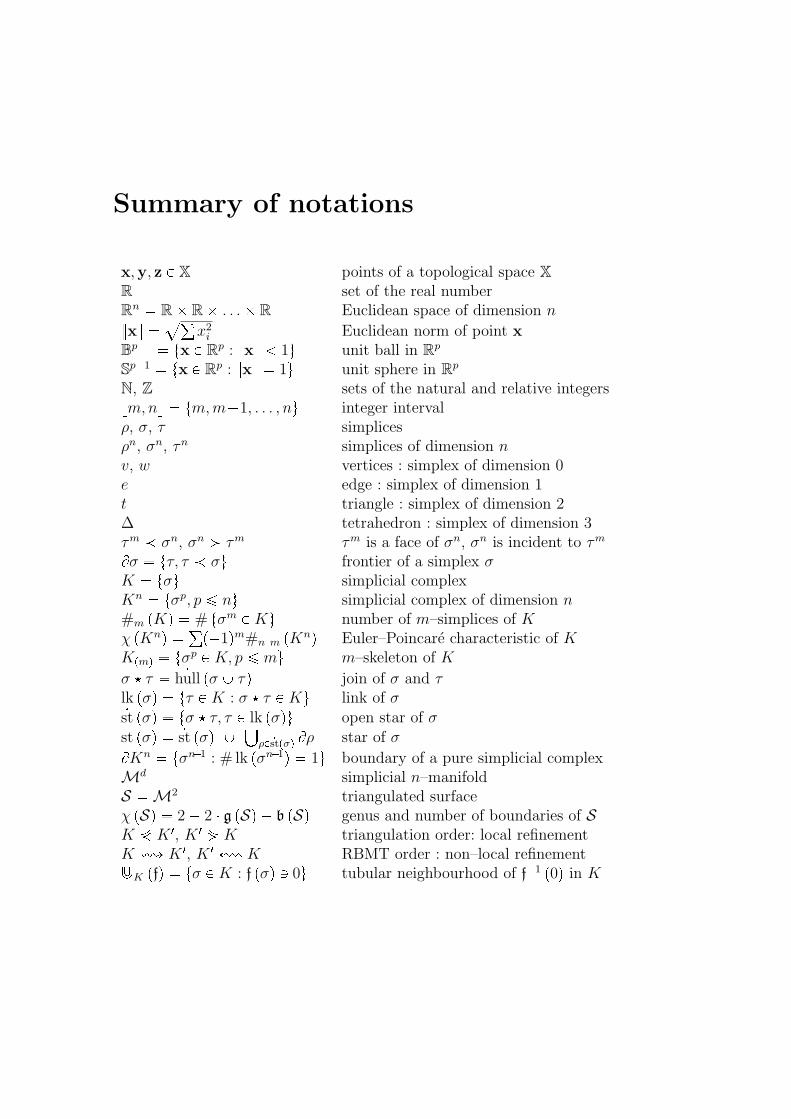
Summary of notations

x,y, z P X points of a topological space XR set of the real numberRn � R� R� . . .� R Euclidean space of dimension n

}x} �a°x2

i Euclidean norm of point xBp � tx P Rp : }x}   1u unit ball in Rp

Sp�1 � tx P Rp : }x} � 1u unit sphere in Rp

N, Z sets of the natural and relative integersvm,nw � tm,m�1, . . . , nu integer intervalρ, σ, τ simplicesρn, σn, τn simplices of dimension nv, w vertices : simplex of dimension 0e edge : simplex of dimension 1t triangle : simplex of dimension 2∆ tetrahedron : simplex of dimension 3τm   σn, σn ¡ τm τm is a face of σn, σn is incident to τm

Bσ � tτ, τ   σu frontier of a simplex σK � tσu simplicial complexKn � tσp, p ¤ nu simplicial complex of dimension n#m pKq � # tσm P Ku number of m–simplices of Kχ pKnq � °p�1qm#n�m pKnq Euler–Poincare characteristic of KKpmq � tσp P K, p ¤ mu m–skeleton of K

σ � τ � 9hull pσ Y τq join of σ and τlk pσq � tτ P K : σ � τ P Ku link of σ9st pσq � tσ � τ, τ P lk pσqu open star of σst pσq � 9st pσq Y �

ρP 9stpσq Bρ star of σ

BKn � tσn�1 : # lk pσn�1q � 1u boundary of a pure simplicial complexMd simplicial n–manifoldS �M2 triangulated surfaceχ pSq � 2� 2 � g pSq � b pSq genus and number of boundaries of SK ¶ K 1, K 1 · K triangulation order: local refinementK ù K 1, K 1 ø K RBMT order : non–local refinement]K pfq � tσ P K : f pσq Q 0u tubular neighbourhood of f�1 p0q in K