MERIT-Infonomics Research Memorandum series

Vintage Modelling for Dummies using the Putty-Practically-Clay Approach Adriaan van Zon

2005-005

MERIT – Maastricht Economic Research Institute on Innovation and Technology PO Box 616 6200 MD Maastricht The Netherlands T: +31 43 3883875 F: +31 43 3884905 http://www.merit.unimaas.nl e-mail:secr-merit@merit.unimaas.nl

International Institute of Infonomics c/o Maastricht University PO Box 616 6200 MD Maastricht The Netherlands T: +31 43 388 3875 F: +31 45 388 4905 http://www.infonomics.nl e-mail: secr@infonomics.nl

Vintage Modelling for Dummies

using the Putty-Practically-Clay Approach

by

Adriaan van Zon

(MERIT, Maastricht, February 2005)

2

1. Introduction

Vintage models have been around for a long time now. Since their conception in

the late Fifties and early Sixties (see, for example, (Jorgenson and W. 1966), (Salter

1960), (Solow 1960; Solow, Tobin et al. 1966)) they have been adopted by economists

interested in the connection between technical change and economic growth, because

they highlight a number of important insights regarding the complementarity between

productivity growth and investment. First of all, productivity growth is positively

influenced by gross investment. In the hitherto standard aggregate production function

approach towards explaining labour productivity growth, the latter was as much the

result of the growth in capital per head (and therefore linked to net investment per head

rather than gross investment), as of (labour saving) technical change itself. And even

though Abramowitz in his reaction to Solow’s paper (Solow 1957) on the contribution of

technical change to productivity growth already noted that the overriding importance of

technical change was also a clear measure of our ignorance, it was only with the advent

of new growth theory in the late Eighties and early Nineties, that economists took up the

challenge implicit in Abramowitz’s remark. In the mean time, i.e. in the late Sixties and

Seventies, economists all over the world had a look at how technical change got diffused

in the economy rather than having a closer look at the sources of technical change.

In the Netherlands in particular, vintage models of production became an integral

part of the policy making models that the Dutch Central Planning Bureau1 used for its

short and medium term policy design. In the Seventies the Netherlands suffered from

the oil-crises because of its very strong dependence on international trade.2 In this

context, the clay-clay vintage model by Den Hartog and Tjan was used to develop a

policy of wage-restraint that could mitigate the employment problems associated with

this period of stagnation. In the process den Hartog and Tjan received only minor

criticism on specific details of their model while criticism on the fundamental vintage

principles of their approach was totally lacking. But soon economists came to the

conclusion that Solow had been more or less right after all (Solow 2000), since much of at

least the flavour of vintage modelling results could be had from far less intricate

aggregate production function models. At the same time much of the burden of

empirically backing the structural parameters of the CPB’s policy models was removed

by switching to using fully forward looking general equilibrium models that were

1 Further called CPB for short. 2 The most important model at the time was the Vintaf-model based on the work by (Den Hartog and Tjan 1979).

3

calibrated rather than econometrically estimated. This general equilibrium focus

required a degree of intertemporal consistency and behavioural completeness that made

the integration of vintage models in such a framework difficult, or at least less of a

priority. Hence, in the Netherlands vintage modelling ran out of fashion, whereas in the

rest of the world it never had been very popular in the first place.

With the revival of growth theory in the Eighties and the Nineties, however,

technical change as such became a hot issue again. Consequently, the factors that could

promote technical change or impede it having its full productivity enhancing effects

became almost equally important. This holds for policy measures that would influence

the incentives underlying the generation of knowledge and hence ultimately technical

change itself, as much as for the vintage idea again, since vintages are the carriers of

technical change on the one hand, as well as the objects of technology specific learning on

the other. So, vintages are instrumental in the realisation of productivity growth. Of

course, economists had known that all along.

Meanwhile the stylised models by (Romer 1990) in which capital was completely

putty, and (Aghion 1992) and Howitt 1992), or (Grossman and Helpman 1991) in which

capital as a factor of production was completely lacking, solved the problem of the

endogeneity of technical change at the expense of providing somewhat of a caricature of

real world investment problems: there is either no problem that can not be completely

fixed ex post (Romer 1990), or there is no investment problem at all because there’s no

investment (Aghion and Howitt 1992) and (Grossman and Helpman 1991). In reality, of

course, investment has the important double role of being the carrier of technical change

and of fuelling the multiplier process.

The relatively recent revival of interest in vintages as carriers of technical change

underlines the new growth theorists’ conclusion that technical change has to be bought

and paid for in a double sense. First the R&D people coming up with the bright ideas

need to be compensated for their efforts (as covered in new growth theory), while

secondly the firms wanting to use these ideas need to be compensated for the costs and

risks involved in using them. Anything that reduces either of these two types of

compensation will have a negative impact on the rate of technical change, either by

slowing down its potential rate, or by slowing down the rate at which the potential is

realised through new investment.

So far, however, the revival of interest in vintage modelling has focussed on the

way in which the lumpiness of investment translates into correspondingly lumpy growth

responses, rather than on integrating endogenous, incentive driven, technical change in

4

a vintage framework. This paper also focuses on the lumpiness of investment, and

especially the practical problems that this entails in integrating a vintage model in a

larger (general equilibrium) ensemble.

There are many different ways in which this has been done so far . These ways

depend to a large extent on the degree of substitution between factors of production after

a vintage has been bought and paid for and the degree of foresight this implies for

making intertemporally consistent investment decisions. With limited substitution

possibilities ex post, profit maximising entrepreneurs also need to make the scrapping

decision an integral part of the investment programs they have to design. This is

discussed in section 2. In section 3 we will describe how such an investment program can

be formulated, and what such an investment program entails for the way in which

output should be produced by the vintages installed in the past and in the present. We

will further illustrate how the various standard scrapping rules used in the vintage

literature follow readily from such an intertemporally consistent investment program.

We also show that Jorgenson’s user cost of capital notion is an integral part of this

program, as well as Amoroso-Robinson pricing behaviour. Section 3 uses a formal putty-

semi-putty model, that has the putty-clay model as a special case. For reasons of

simplicity, we use continuous time vintages. In practice, however, model builders

generally use discrete time vintages. In combination with explicit scrapping behaviour,

this may lead to numerical difficulties, since the aggregate supply curve can become

locally infinitely elastic, sometimes precluding finding a simultaneous numerical

solution for the entire model rather than just for the vintage production model. In

section 4, we will suggest a way around this problem that hinges on the notion of

practically (but not totally) zero ex post substitution possibilities between the various

factors of production. This gives rise to our ‘putty-practically-clay’-model. In section 5 we

show how this model performs relative to a full putty-clay vintage model with

‘Malcomson-scrapping’.3 Section 6 summarises the results.

3 Malcomson, J. M. (1975) was the first to come up with a scrapping rule that maximises integral profits over all vintages taken together, regardless of the degree of competition on the output market.

5

2. Vintage modelling

General background

A vintage model is based on the notion of investment as a vehicle for the

transmission of technical change. Technical change comes in two varieties, i.e. as

improved or totally new products, or as improved organisation of a production process (or

a combination of both). A new product that incorporates technical change is said to

reflect embodied technical change. Efficiency improvements due to better organisation or

learning are said to be the result of disembodied technical change.

The significance of the notion of embodied technical change lies in the fact that in

order to experience productivity growth, one actually has to buy and use the new

products (in this case investment goods) that embody the latest production technologies.

Embodied technical change is therefore certainly and explicitly not a free good falling

like ‘manna from heaven’. In the case of investment in new production technologies, this

automatically implies that not ‘technological change ’ per se drives productivity growth,

but also the conditions under which investment will take place, among which the user

cost of capital, demand expectations, the degree of competition, and so on.

Vintage models come in a number of varieties depending on the degree to which

factors of production can be substituted. In the life of a vintage, there are three distinct

phases to take into account, i.e. the investment phase, the production phase and the

scrapping phase. During the investment phase, entrepreneurs can choose between

different implementations of the latest production technologies. These implementations

differ with respect to unit factor requirements, usually a fixed factor like capital and a

variable factor like labour. Depending on the degree of substitution between the

respective factors of production one categorises this phase as clay for no substitution

possibilities (fixed proportions) or putty (for ‘ample’ substitution possibilities as implied

by a neo-classical production function, for instance). The investment phase is often

described as the situation before the production phase when the (initial) characteristics

of a vintage of investment goods have to be decided upon. This is called the ex ante

situation.

In the production phase, factor proportions can either be fixed (clay again) or

flexible (putty), or reasonably flexible but less so than ex ante (semi-putty). The

combination of different degrees of flexibility of factor proportions for the situations ex

ante and ex post (after the decision which implementation of new technology to buy)

gives rise to different types of vintage models. The most important ones are clay-clay,

6

putty-clay, and putty-putty models. Clay-putty models do not exist. The first clay or

putty refers to the situation ex ante, and the second one to the situation ex post.

The decisive difference between a clay situation and a putty situation is that in

the former case one has to forecast price-developments of the factors of production. For,

fixed proportions ex post do not allow one to change factor proportions when something

happens to relative prices: if one chooses certain factor proportions ex ante, one has to

live with the cost-consequences ex post. In a putty ex post situation, one can simply

substitute away from the factors that have become relatively expensive. One usually

regards putty-clay production models to be the most realistic versions of a vintage model.

The clay ex post feature of a putty-clay model also points to the problem of

deciding when to stop using a certain vintage, since with fixed factor proportions ex post,

but with increasing (total-) factor productivity ex ante, the productivity difference

between ‘old’ and ‘new’ equipment grows over time. And one can easily imagine this

productivity difference to become so large that at some point in time it would be better to

transfer production from old equipment to new equipment. This decision belongs to the

third phase mentioned above, i.e. the scrapping phase. Scrapping refers to the laying off

of old equipment, even if it is not totally worn down, for economic reasons. Due to

embodied technical change it is even possible to improve the gross rate of return on

overall investment by re-allocating variable resources from older vintages to the newest

vintage. There are two ways in which this can be done:

1. By avoiding operating losses on old equipment (i.e. by avoiding negative quasi-rents4

by scrapping the vintages with a negative quasi-rent ex post (further called the non-

negative quasi-rent condition));

2. By shifting the production of output from old vintages with a gross operating surplus

that is below the net operating surplus of the newest vintage to the newest vintage

(thus maximising integral profits). The condition that states that vintages with a low

but positive quasi-rent should be scrapped in favour of the new vintage if the latter

generates a rent larger than the quasi-rent of the old vintage under consideration is

called the Malcomson condition.

Both ways imply the same kind of behaviour in a perfect competition setting, because

in that case the price of output reflects the marginal cost of producing output, i.e. the

4 The quasi-rent of a vintage is the gross operating surplus on that vintage, i.e. the value of sales less the hiring costs of the variable inputs.

7

total unit costs on the newest vintage. We will describe the connections between these

scrapping rules in more detail in the next section.

Vintage modelling problems

There are two practical problems associated with the use of putty-clay vintage

models, i.e. the type of vintage model that is considered to be the most relevant in

practice. The first is that the characteristics (factor proportions) of a vintage must be

determined on the basis of expectations about the future development of factor prices. Ex

post these expectations may prove to be correct or not. In any case, the actual

profitability of a vintage is only known ex post, and so in order to be able to tell how big

total profitable capacity is at some moment in time, a comprehensive bookkeeping

system is needed of all vintages that add to total production capacity.

The second problem is connected with scrapping as such and therefore with a clay

ex post situation.5 When a vintage generates a negative quasi-rent or a sub-optimal

quasi-rent, that vintage would be scrapped by rational, profit maximising entrepreneurs.

The problem is now that for a small drop in the price of final output, a relatively large

volume reaction can occur if the vintage to be scrapped is, for some historical reason,

relatively big. In that case, the supply curve of productive capacity may become ‘near

infinitely elastic’ at the final output price under consideration. This can lead to

numerical difficulties, if only because of the discontinuities in the supply response to

small price changes, and certainly so in a setting where the solution of a model is

obtained through Gauss-Seidel iterations or something similar. In that case alternating

behaviour can arise that is first of all unrealistic and secondly precludes the quick

convergence of the model solution.

The solution to the bookkeeping problem is to drop the assumption of the

scrapping of vintages, i.e. to have either a putty-(semi-)putty model as in (Zon 1994), for

example, or something like a (Bischoff 1971) model, which is nominally putty-clay but

that lacks the actual scrapping behaviour that is implied by a clay ex post situation and

the assumption of economic rationality in investment behaviour. The lack of explicit

scrapping behaviour enables one to use a set of recursive update rules for aggregate

factor productivity in function of the rates of embodied factor augmenting technical

change and the share of new investment in the total capital stock. In such a case it is not

necessary to keep track of all individual vintages; keeping track of only the newest

5 In a (semi-) putty ex post situation, ‘scrapping’ takes an entirely different form. We will come back to this later.

8

vintage and the set of all old ones taken together will suffice.6 Naturally, by adopting the

Bisschoff solution, one is also ‘throwing the baby out with the bath-water’, since one of

the most important reasons to use the vintage model in the first place is the

heterogeneity of vintages in terms of their productive characteristics and its implication

for the duration of their profitable use. In addition to this, technical change itself has a

direct impact on economic lifetime in the context of the Malcomson scrapping condition

(see, for example, (Zon 1991) for this connection). In the case of technological shocks, the

induced scrapping of old equipment (the equivalent of Schumpeterian creative

destruction) makes room for newer equipment, and so leads to a faster diffusion of the

new technology, and a faster realisation of the productive potentials locked up in the

newest vintages of investment equipment. Dropping the scrapping condition then

ignores one of the main channels through which technological change makes itself felt,

i.e. the restructuring of productive capacity in times of rapid technological change.

So, discarding the Bisschoff solution and opting for a putty-clay approach, the

only problem left is the discontinuity problem. We can fix that problem either by making

investment more continuous or by making scrapping less discontinuous. In the modern

vintage literature7 focussing on the impact of vintage investment on real business cycles,

one usually opts for making investment responses more continuous through assumptions

that allow for heterogeneity of productivity characteristics within vintages rather than

just between vintages. In this way only parts of a vintage will be scrapped, and the

response to changing scrapping incentives will become smoother than with homogeneous

vintages. A slightly different approach to making the volume response to supply price

changes somewhat more continuous has been suggested by (Muysken and Zon 1987).

They assume that the characteristics of a vintage are spread over a region in unit-factor-

requirement-space rather than being concentrated in just one point of that space,

because entrepreneurs are intrinsically heterogeneous resulting in different expectations

regarding relative factor prices or different intensities of their reactions to such

expectations. This implies that for small changes in final output prices, the

corresponding supply reaction will be much smoother than before, since just a subset of

all the entrepreneurs that have invested in a vintage may have to decide to discard the ir

share in the vintage under consideration.

6 See, for example, (Italianer 1984) and (van Zon 1994). 7 See, for example, (Greenwood, Hercowitz and Huffman 1988), (Cooper, Haltiwanger and Power 1999), (Gilchrist and Williams 2000) and (Campbell 1998) for such links between business-cycles and investment.

9

Finally, a solution to the discontinuity problem is to allow for non-zero but (very)

limited substitution possibilities ex post. By doing this, the gross rate of return on a

vintage can be made infinitely high by raising the marginal productivity of the variable

factor by ever increasing the capital intensity of production.8 Obviously, since capital is a

fixed factor of production and both factors of production are necessary to produce output,

the asymptotic vanishing of the variable factor also makes output on that vintage

vanish, thus effectively (but at least continuously) mimicking the scrapping of production

capacity.

In order to illustrate the principles involved, we will formulate a continuous time

putty-semi-putty model, based on CES production functions ex ante and ex post. This is

the subject of the next section.

3. A continuous time putty-semi-putty vintage model

3.1 Introduction

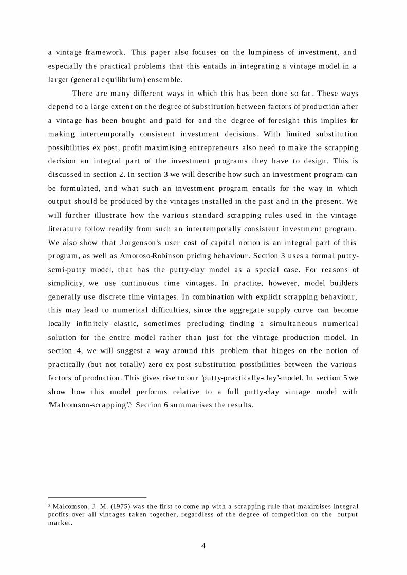
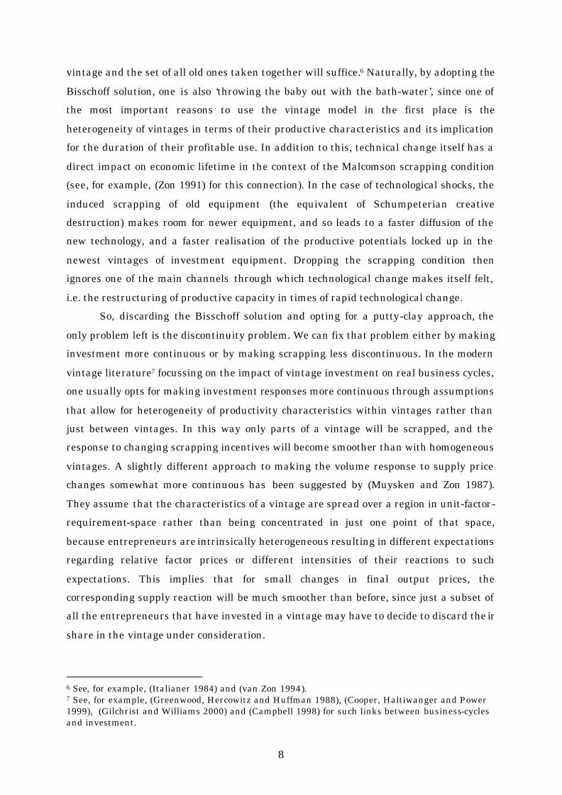
In Figure 1 below, we have depicted a putty-semi-putty production structure. The

solid convex curve through points A and B is the unit iso-quant describing how much of

the fixed factor (denoted by k) and of the variable factor (denoted by v) should be

combined to produce one unit of output. This curve is the convex hull of numerous

technologies that each have relatively limited substitution possibilities. Two of these

technologies have been depicted using dotted curved lines in the Figure. They have the

points A and B in common with their convex hull. They will further be called

technologies A and B. A putty-clay model is a special case of this set-up, since in that

case substitution possibilities ex post are zero by assumption. This is indicated, for

example, by the solid rectangular iso-quant touching the hull in point A.9 This means

that technology A effectively consists of just one technique, and so substitution between

techniques (or moving along an iso-quant) is not possible due to either the nature of the

technology itself or the incompleteness of human knowledge.

It should be noted that this convex hull is a kind of short-hand notation for all the

technologies that an entrepreneur can choose from. But once a particular technology

like A or B has been chosen, further selections of techniques belonging to technologies

A and B are limited to the ones represented by the dotted unit iso-quants through points 8 This assumes that the Inada conditions still apply in this case. 9 In a CES setting, the ex post iso-quant can be made to approach the rectangular iso-quant by choosing a value of the elasticity of substitution that is close to zero.

10

A and A’ or through points B and B’. The dotted unit iso-quants can therefore be thought

of as collections of (slightly) different implementations of a particular technology. It

should finally be noted that due to embodied factor augmenting technical change, the

convex hull shifts in the direction of the origin. If factor augmenting technical change

would be k-biased, then it shifts more in the direction of the k-axis than in the direction

of the v-axis, and the other way around, mutatis mutandis.

Figure 1. A putty-semi-putty production structure

Technology A is relatively v-intensive implying that for the same relative prices,

as is the case in points A’ and B’, for example, the v/k-ratio in point A’ is higher than the

v/k-ratio in point B’. Hence, an entrepreneur who would expect the relative price of k to

be generally low would be better off choosing technology B, and an entrepreneur who

would expect the relative price of v to be low, would do better choosing technology A.

This follows directly from the interpretation of the slope of the straight lines through

points A’, B’ and B’’ as the relative factor prices of the factors v and k. In that case, the

intercepts of the straight lines with the vertical are a direct measure of the total cost of v

and k taken together. In that case point A’ represents a higher cost level than point B’,

even though relative prices are the same in points A’ and point B’ (i.e. at relatively low

relative prices for factor k). So why would technology A then ever be chosen? The answer

is that entrepreneurs may expect factor prices to change ex post. And A would be the

C’

B’

B’’

A’

B

A

v

k

C

11

preferred technology if the factor price of v would be expected to be relatively low, even

though it may be at a relatively high level at the moment the vintage is installed, as

given by the slopes of the iso-cost lines through points B’ and A’, for example. So if the

relative price of v is initially high but is also expected to be permanently much lower in

the near future, them technology A is preferred to B by rational entrepreneurs.

If we would be using CES functions to describe both the ex ante unit-isoquant

through points A and B (that is the convex hull of all individual technologies that are

best practice at some point in time), and the unit iso-quants of all individual technologies

like A and B, then the position of the individual technologies A and B in the factor

coefficient space depends on the way in which the convex hull has been parameterised.

In the context of a CES function, the general shape of the unit-isoquant depends the

elasticity of substitution and the distribution coefficients. The values of these

parameters implicitly define the position of the individual technologies A and B (and all

other technologies supported by the hull). In addition to this, the shape of the individual

technologies is of course defined by the elasticity of substitution associated with each

individual technology. Take technology A, for example. Its distribution coefficients are

completely determined by the requirements that the ex ante function and the ex post

function must have a value equal to 1 in point A. Moreover, the slopes of the straight

lines that are tangent in A with both the ex ante and the ex post unit iso-quants should

be the same. These requirements are sufficient to define the ex post distribution

coefficients of A in terms of the distribution coefficients of the ex ante function and the

value of the v/k-ratio in point A. We will call this value of the v/k-ratio the ‘tangential

technique’. Obviously, for technology B, the distribution coefficients would be defined in

terms of the ex ante distribution coefficients and the v/k-ratio in point B.

The problem of choosing a technology to invest in then boils down to making two

‘sub-choices’: first the choice of an individual technology (like the unit ex post iso-quant

going through point B), and secondly a specific implementation of that technology (or

individual techniques like B’ or B’’). In order to show how this works, we will have to

specify the ex ante and ex post functions, after which we can specify the general

investment problem and its solution. This is the subject of the following sub-paragraphs.

12

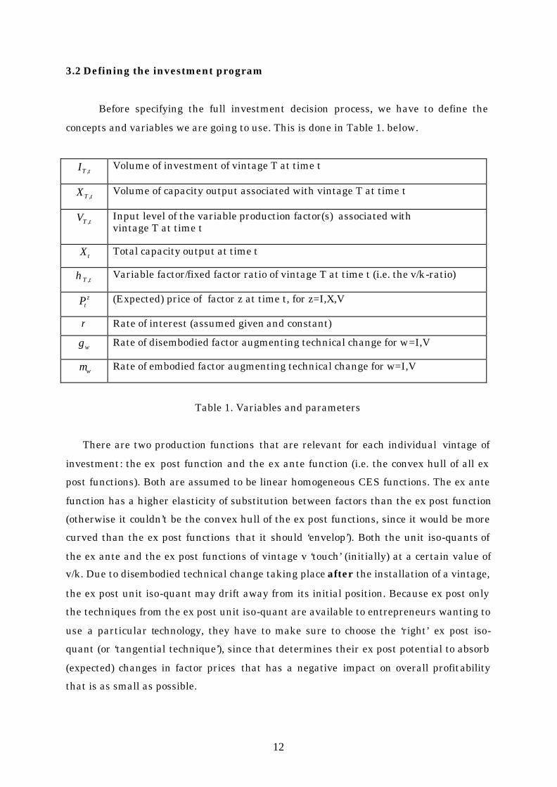
3.2 Defining the investment program

Before specifying the full investment decision process, we have to define the

concepts and variables we are going to use. This is done in Table 1. below.

tTI , Volume of investment of vintage T at time t

tTX , Volume of capacity output associated with vintage T at time t

tTV , Input level of the variable production factor(s) associated with vintage T at time t

tX Total capacity output at time t

tT ,η Variable factor/fixed factor ratio of vintage T at time t (i.e. the v/k-ratio)

ztP (Expected) price of factor z at time t, for z=I,X,V

r Rate of interest (assumed given and constant)

wγ Rate of disembodied factor augmenting technical change for w=I,V

wµ Rate of embodied factor augmenting technical change for w=I,V

Table 1. Variables and parameters

There are two production functions that are relevant for each individual vintage of

investment: the ex post function and the ex ante function (i.e. the convex hull of all ex

post functions). Both are assumed to be linear homogeneous CES functions. The ex ante

function has a higher elasticity of substitution between factors than the ex post function

(otherwise it couldn’t be the convex hull of the ex post functions, since it would be more

curved than the ex post functions that it should ‘envelop’). Both the unit iso-quants of

the ex ante and the ex post functions of vintage v ‘touch’ (initially) at a certain value of

v/k. Due to disembodied technical change taking place after the installation of a vintage,

the ex post unit iso-quant may drift away from its initial position. Because ex post only

the techniques from the ex post unit iso-quant are available to entrepreneurs wanting to

use a particular technology, they have to make sure to choose the ‘right’ ex post iso-

quant (or ‘tangential technique’), since that determines their ex post potential to absorb

(expected) changes in factor prices that has a negative impact on overall profitability

that is as small as possible.

13

As regards this profitability, we assume now that entrepreneurs want to maximise

the present value of the rents they can obtain by investing in a certain technology and

then using that technology as an integral part of their ‘vintage-portfolio’ to produce an

aggregate volume of output needed to service demand. The decision how much to invest

and in which ex post unit iso-quant to invest is made conditional on the requirement

that the specific vintage investment is part of a complete intertemporal investment

program10 with the aim of maximising the present value of the flow of rents that can be

obtained from the vintage portfolio. In order to derive this investment program, we

postulate the following ex ante and ex post production functions:

( ) ααα /1

,,,,, ),(−−−

⋅+⋅== TTTTTTTTTTTTT VBIAVIgX (1.A)

( ) TtVDICVIfX tTtTtTtTtTtTtTtT ≥∀⋅+⋅==−−− βββ /1

,,,,,,,, ),( (1.B)

In (1.A), )1/(1 ασ +=a is the elasticity of substitution of the ex ante function gT(), while

)1/(1 βσ +=p is the elasticity of substitution of the ex post function fT,t() (cf. (1.B)). In

equation (1.A), AT and BT are the ex ante distribution parameters that may change over

time (and so differ between technologies) due to embodied technical change, i.e.:

TT

IeAA⋅

⋅=µ

0 (1.C)

T

TVeBB

⋅⋅=

µ0 (1.D)

Due to technical wear and tear, the amount of capital associated with a particular

vintage gradually decays over time. We assume radioactive decay at a common rate δ

for all vintages. Thus we get:

TteII TtTTtT ≥∀⋅= −⋅− )(,,

δ (2)

Because of the linear homogeneity of (1.A) and (1.B) we must have:

10 An investment program is a sequence of investment decisions that optimises some objective function.

14

),(1 ,, TTTTT vkg= (3.A)

),(1 ,,, tTtTtT vkf= (3.B)

where kT,t and vT,t are capital per unit of capacity output and the variable factor per unit

of capacity output of vintage T at time t. Initially, the two unit iso-quants should be

tangent at the tangential technique given by TTTTTT vk ,,, /=η . In addition, the slopes of

both unit iso-quants should be the same for the tangential technique TT ,η . Hence we

obtain the following constraints on gT () and fT,t():

1),(),( ,,,,, == TTTTTTTTTTT vkfvkg (4.A)

TT

TT

TT

TT

TT

T

TT

T

vf

kf

vg

kg

,

,

,

,

,,

//∂∂

∂∂

=∂∂

∂∂

(4.B)

where (4.B) can be derived from the equal slopes requirement. (4.A) and (4.B) provide

two equations that can be used to link the ex post distribution parameters to the ex ante

distribution parameters for a given tangential technique TTTTTT vk ,,, /=η and for given

values of the substitution parameters α and β . We get:

( ) ββαβα /)(,

/,

−⋅= TTTTT kAC (5.A)

( ) ββαβα /)(,

/,

−⋅= TTTTT vBD (5.B)

(5.A) and (5.B) describe the initial values of the ex post distribution parameters. These

can change due to disembodied technical progress. It should be noted that the ex post

parameters are equal to their ex ante counterparts if the elasticities of substitution ex

ante and ex post are the same, as it should be in that case. Because of disembodied factor

augmenting technical change at given rates Iγ and Vγ , we have furthermore:

15

)(,,

TtTTtT

IeCC −⋅⋅= γ (6.A)

)(,,

TtTTtT

VeDD −⋅⋅= γ (6.B)

The instantaneous flow of quasi-rents associated with investment in a certain

vintage T at time t is now given by:

tTV

ttTX

ttT VPXPQR ,,, ⋅−⋅= (7)

It should be noted that from a vintage point of view there are two types of

instrumental variables: those that can be determined only once (like the initial level of

investment associated with a vintage, as well as the corresponding tangential techniques

of that vintage), and those that can be adjusted ex post, like the ex post factor coefficient

(and hence output too for an ex post given volume of investment). A third type of variable

is non vintage-specific. In this particular case that would be the price of output (this

assumes that output produced on all vintages is homogeneous). In equation (7), the

‘adjustable’ instrumental variables for time t are the price of output XtP , capacity output

of the existing vintages XT,t and the amount of the variable factor per vintage, VT,t. For

the time of installation of the vintage T, the ‘one shot’ instrumental variables are the

volume of investment at time T, i.e. TTI , , but also the tangential technique

TTTTTT vk ,,, /=η that defines both the shape and the location in factor-space of the ex post

production function fT,t().

The demand for output Dt is assumed to be given by a constant price-elasticity of

demand function:

( ) ε−⋅= X

ttt pZD (8)

where Zt is an autonomous scale factor that may change over time, and where ε is a

constant number greater than 1.

For reasons of simplicity and expositional purposes we now assume that

investment decisions are taken continuously, rather than at one-year intervals.

Furthermore, taking time t to refer to the present, we now want to find the investment

program that maximises the present value of all current and future rent streams

associated with all presently existing vintages and all the vintages still to be installed.

16

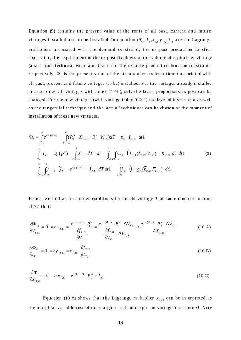
Equation (9) contains the present value of the rents of all past, current and future

vintages installed and to be installed. In equation (9), ttvtvt ϕψξλ ,,, ,, are the Lagrange

multipliers associated with the demand constraint, the ex post production function

constraint, the requirement of the ex post fixedness of the volume of capital per vintage

(apart from technical wear and tear) and the ex ante production function constraint,

respectively. tΦ is the present value of the stream of rents from time t associated with

all past, present and future vintages (to be) installed. For the vintages already installed

at time t (i.e. all vintages with index tT < ), only the factor proportions ex post can be

changed. For the new vintages (with vintage index tT ≥ ) the level of investment as well

as the tangential technique and the ‘actual’ techniques can be chosen at the moment of

installation of these new vintages.

( )

( ) ( )∫∫∫

∫∫∫ ∫

∫∫

∞

=−∞=

−⋅−∞

=

−∞=

∞

=

∞

= −∞=

−∞=

∞

=

−⋅−

−⋅+−⋅⋅

+−⋅+

−⋅

+

⋅−⋅−⋅⋅=Φ

tttttttt

t

TtT

TtTTtT

tt

t

TtTtTtTtTtT

tttt

t

TtT

xttt

t

Ttt

IttT

VttT

Xt

tt

ttrt

dtvkgdtdTIeI

dtdTXVIfdtdTXpD

dtIpdTVPXPe

11,11,111

1

1,)1(

,1,1

1

1,1,1,1,1,11

1

1,111

1

1,111,11,11

)1(

1),(11

1),()(

1)(

ϕψ

ξλ

δ

(9)

Hence, we find as first order conditions for an old vintage T at some moment in time

tt ≥1 that:

1,

1,1)1(

1,1,

1,

1,1)1(

1,

1,

1)1(

1,1,

1 0tT

tTV

tttr

tTtT

tT

tTV

tttr

tT

tT

Vt

ttr

tTtT

t

XVPe

VVf

VPe

Vf

PeV ∆

∆⋅⋅≈

∆⋅∂∂

∆⋅⋅=

∂∂

⋅==>=

∂Φ∂ −⋅−−⋅−−⋅−

ξ (10.A)

1,

1,1,1,

1,

1 0tT

tTtTtT

tT

t

If

I ∂∂

⋅==>=∂Φ∂

ξψ (10.B)

11)1(

1,1,

0 tX

tttr

tTtT

t PeX

λξ −⋅==>=∂

Φ∂ ⋅−− (10.C)

Equation (10.A) shows that the Lagrange multiplier 1,tTξ can be interpreted as

the marginal variable cost of the marginal unit of output on vintage T at time t1. Note

17

that (10.C) should hold for all 1tT ≤ . Moreover, the RHS of (10.C) is independent of T,

and so it must be the case that 11,11, tTtttT ≤∀= ξξ . Hence on old and new vintages the

variable factors should be employed up to the point where their marginal product is the

same on all vintages.

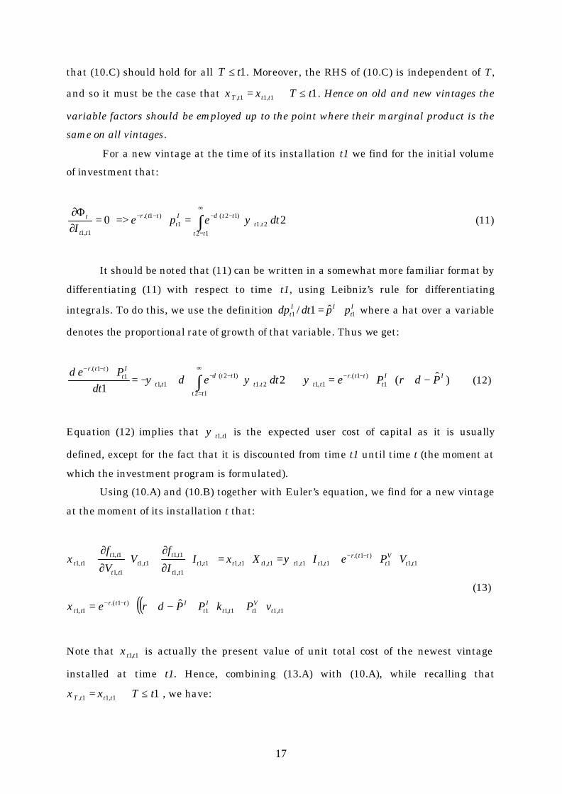
For a new vintage at the time of its installation t1 we find for the initial volume

of investment that:

2012

2.1)12(

1)1.(

1,1

dtepeI tt

ttttI

tttr

tt

t ∫∞

=

−⋅−−− ⋅=⋅=>=∂

Φ∂ψδ (11)

It should be noted that (11) can be written in a somewhat more familiar format by

differentiating (11) with respect to time t1, using Leibniz’s rule for differentiating

integrals. To do this, we use the definition It

IIt ppdtdp 11 ˆ1/ ⋅= where a hat over a variable

denotes the proportional rate of growth of that variable. Thus we get:

)ˆ(21 1

)1.(1,1

122.1

)12(1,1

1)1.(

IIt

ttrtt

tttt

tttt

It

ttr

PrPedtedt

Ped−+⋅⋅=⇔⋅⋅+−=

⋅ −−∞

=

−⋅−−−

∫ δψψδψ δ (12)

Equation (12) implies that 1,1 ttψ is the expected user cost of capital as it is usually

defined, except for the fact that it is discounted from time t1 until time t (the moment at

which the investment program is formulated).

Using (10.A) and (10.B) together with Euler’s equation, we find for a new vintage

at the moment of its installation t that:

( )( )1,111,11)1.(

1,1

1,11)1.(

1,11,11,11,11,11,1

1,11,1

1,1

1,11,1

ˆtt

Vttt

It

Ittrtt

ttV

tttr

tttttttttttt

tttt

tt

tttt

vPkPPre

VPeIXII

fV

V

f

⋅+⋅⋅−+⋅=

⇒⋅⋅+⋅=⋅=

⋅

∂

∂+⋅

∂

∂⋅

−−

−−

δξ

ψξξ

(13)

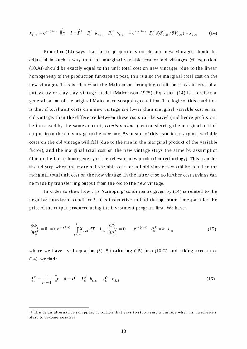
Note that 1,1 ttξ is actually the present value of unit total cost of the newest vintage

installed at time t1. Hence, combining (13.A) with (10.A), while recalling that

11,11, tTtttT ≤∀= ξξ , we have:

18

( )( ) 1,1,1,1)1.(

1,111,11)1.(

1,1 )//(ˆtTtTtT

Vt

ttrtt

Vttt

It

Ittrtt VfPevPkPPre ξδξ =∂∂⋅=⋅+⋅⋅−+⋅= −−−− (14)

Equation (14) says that factor proportions on old and new vintages should be

adjusted in such a way that the marginal variable cost on old vintages (cf. equation

(10.A)) should be exactly equal to the unit total cost on new vintages (due to the linear

homogeneity of the production function ex post, this is also the marginal total cost on the

new vintage). This is also what the Malcomson scrapping conditions says in case of a

putty-clay or clay-clay vintage model (Malcomson 1975). Equation (14) is therefore a

generalisation of the original Malcomson scrapping condition. The logic of this condition

is that if total unit costs on a new vintage are lower than marginal variable cost on an

old vintage, then the difference between these costs can be saved (and hence profits can

be increased by the same amount, ceteris paribus ) by transferring the marginal unit of

output from the old vintage to the new one. By means of this transfer, marginal variable

costs on the old vintage will fall (due to the rise in the marginal product of the variable

factor), and the marginal total cost on the new vintage stays the same by assumption

(due to the linear homogeneity of the relevant new production technology). This transfer

should stop when the marginal variable costs on all old vintages would be equal to the

marginal total unit cost on the new vintage. In the latter case no further cost savings can

be made by transferring output from the old to the new vintage.

In order to show how this ‘scrapping’ condition as given by (14) is related to the

negative quasi-rent condition11, it is instructive to find the optimum time-path for the

price of the output produced using the investment program first. We have:

11)1.(

1

11

1

1,)1.(

1

00 tX

tttr

Xt

tt

t

TtT

ttrX

t

t PePD

dTXeP

λελ ⋅=⋅⇒=∂∂

⋅−⋅=>=∂

Φ∂ −−

−∞=

−− ∫ (15)

where we have used equation (8). Substituting (15) into (10.C) and taking account of

(14), we find:

( )( )1,111,111ˆ

1 ttV

tttI

tIX

t vPkPPrP ⋅+⋅⋅−+⋅−

= δε

ε (16)

11 This is an alternative scrapping condition that says to stop using a vintage when its quasi-rents start to become negative.

19

Equation (16) reproduces the Amoroso-Robinson condition for the profit maximising

price of output under imperfect competition. If the price elasticity of demand is infinitely

high (as it would be the case in a perfectly competitive environment), then the optimum

price just covers marginal total cost, and hence equation (14) would in this case be

reduced to the non-negative quasi-rent condition. This follows readily from the fact that

in that case the price of output would equal total unit cost on the newest vintage, and so

equation (14) states that the variable factor should be adjusted up to the point where the

marginal variable costs just equal the price of output (and hence (marginal) quasi-rents

on the old vintages are zero). Note that in the case of a putty-clay model, this rule

implies that the allocation of the variable factor to machinery of an old vintage should be

reduced as long as its marginal variable cost exceeds the price of output. Since in a

standard putty-clay model the factor productivities ex post are independent of the level

of use of the factors under consideration, this means that the input of the variable factor

should be reduced to a zero level, hence effectively ‘scrapping’ the entire vintage.

We conclude then that equation (14) generates qualitatively the same results as the

scrapping rules one normally encounters in clay-ex-post vintage models. Equation (14) is

conceptually similar, but is more general since it covers putty-semi-putty models as well.

Moreover, equation (14) has the benefit of resulting from a general intertemporal

optimisation problem rather than being postulated a priori.

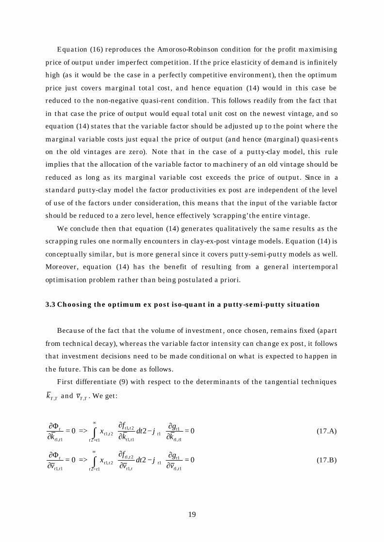
3.3 Choosing the optimum ex post iso-quant in a putty-semi-putty situation

Because of the fact that the volume of investment, once chosen, remains fixed (apart

from technical decay), whereas the variable factor intensity can change ex post, it follows

that investment decisions need to be made conditional on what is expected to happen in

the future. This can be done as follows.

First differentiate (9) with respect to the determinants of the tangential techniques

TTk , and TTv , . We get:

0201,1

11

12 1,1

2,12,1

1,1

=∂∂

⋅−∂∂

⋅=>=∂

Φ∂∫∞

= tt

tt

tt tt

tttt

tt

t

kg

dtkf

kϕξ (17.A)

0201,1

11

12 ,1

2,12,1

1,1

=∂∂

⋅−∂∂

⋅=>=∂

Φ∂∫∞

= tt

tt

tt tt

tttt

tt

t

vg

dtvf

vϕξ (17.B)

20

Because of the linear homogeneity of the ex ante function )(tg , we also find that:

212

1,11,1

2,11,1

1,1

2,12,11 dtk

kf

vvf

tttt

tt

tttt

tt

ttttt ∫

∞

=

∂∂

+∂∂

⋅= ξϕ (18)

Using equations (1.B), (1.C), (1.D), (5.A),(5.B),(6.A), (6.B) and the requirement

that 11,11, tTtttT ≤∀= ξξ , and taking account of (13), it follows that (18) can be written as:

212

2,12,11 dtXtt

ttttt ∫∞

=

⋅⋅−

= ξβ

βαϕ (19)

It follows from (19) that 1tϕ is proportional to the present value of the cost

associated with producing output on the vintage installed at time t during its entire

(infinite) lifetime. It should be noted that the bigger the difference is between the

elasticities of substitution ex ante and ex post, the larger 1tϕ will be. In the putty-putty

case we have 101 tt ∀=⇒= ϕβα . In this case substitution possibilities ex post are as

large as those ex ante, and so an optimum tangential technique does not exist. Equation

(19) by itself is of little real help in determining the optimum tangential technique ,

though. But equations (10.A) and (10.B) in combination with (17.A) and (17.B) provide

the information we need. Taking the ratio of equations (17.A) and (17.B), we find:

α

α

ψ

ξ

ξ

/1

122,12

)12.(

122,12,1

1

1

1,1

1,1

1,112

2,12,1

1,112

2,12,11

1,1

1,1

1

1

1,11

1,11

2

2

2/

2/

//

−

∞

=

−−

∞

=

∞

=

∞

=

−−

⋅⋅

⋅=

⇒∂∂⋅

∂∂⋅=

⋅=

∂∂∂∂

∫

∫

∫

∫

dtVpe

dtI

AB

vk

dtvf

dtkf

vk

BA

vgkg

tttt

Vt

ttr

tttttt

t

t

tt

tt

tttt

tttt

tttt

tttt

tt

tt

t

t

ttt

ttt

(20)

Equation (20) can be obtained by substituting (10.A) and (10.B) into (17.A) and

(17.B), while noting that the marginal products of the tangential techniques can be

21

related directly to the ex post marginal productivities of capital and the variable

factor(s). Equation (20) shows that the capital intensity of the optimum tangential

technique depends negatively on the ratio of the present value of the total capital costs

associated with a vintage (i.e. the numerator of the last part of equation (20)) and the

present value of total variable costs necessary to use the vintage (i.e. the denominator of

the last part of equation (20)).

In order to fully solve equation (20) for the tangential technique, we need to solve

two other ‘problems’ first. We need to find the value of 2,1 ttψ and also the value of

2,12,1 / tttt IV . This follows immediately from the fact that we can write the second part of

(20) as:

α

δ

δψ/1

122,12,1

)12).(ˆ(1

)12.(

12

)2(2,1

1

1

1,1

1,1

2)/(

2−

∞

=

−−+−−−

∞

=

−⋅−

⋅⋅

⋅=

∫

∫

dtIVePe

dte

AB

vk

tttttt

ttPrVt

ttr

tt

tttt

t

t

tt

tt

V

(21)

It should be noted that the integral in the numerator of the RHS of (21) is exactly

equal to the present value price of capital (see equation (11)), whereas 2,12,1 / tttt IV can be

obtained by evaluating the ratio of equations (10.A) and (10.B):

2,1

2)12.(

1

2,1

2,1

2,1

2,1

2,12,1

2,12,1

//

tt

Vt

ttr

tt

tt

tt

tt

tttt

tttt PeIV

CD

IfVf

ψ

β⋅

=

⋅=

∂∂∂∂ −−

−−

(22)

where it should be noted that the ex post distribution parameters Ct1,t2 and Dt1,t2 depend

on the tangential technique again. It follows from (22) that we need to know what 2,1 ttψ

looks like.

Let us assume now that )12(ˆ1,12,1

tttttt e −⋅⋅= ψψψ . Substituting this into equation (11),

we find that:

1,1)1.(

1,112

)12().ˆ(1,1

12

)12(2,1 )ˆ()ˆ/(22 tt

It

ttrtt

tt

tttt

tt

tttt Pedtedte ψψδψδψψψ ψδδ =−⋅⋅⇒−=⋅=⋅ −−

∞

=

−⋅−−∞

=

−⋅− ∫∫ (23)

22

Obviously, (23) and (12) taken together imply that rP I −= ˆψ . Substituting the latter

result into (22), we get:

2,1

)1/()(

1,1

1,1

)1/(1

12,1

)12).(ˆˆ(12,1

2,1

2,1

)ˆ( tttt

ttII

ttt

ttPPVttt

tt

tt

kv

PrPDePC

IV

IV

Ω⋅

=

−+⋅⋅⋅⋅

=

+−+−

−− ββαβ

δ (24)

where we have defined:

)1/(1

11

)12)).(.(ˆˆ(11

2,1)ˆ(

βγγβ

δ

+−−−−−

−+⋅⋅⋅⋅

=ΩII

tt

ttPPVtt

ttPrPA

ePB IVIV

(25)

Substituting (24) and (25) into (21), and solving for the tangential technique, we

finally obtain:

1

)1/(1

/1

/)1(

1

1

1

1

1,1

1,1 )ˆ(1

ˆ)ˆ()()1(t

IIV

IVV

t

It

t

t

tt

tt WPrPPr

PP

AB

vk

=

−+⋅

+−−−⋅++⋅+

⋅⋅

=

+−

−

+− α

β

ββα

δβ

γγβδβ

(26)

Equation (26) shows how the elasticity of substitution and the distribution

parameters of the ex ante function, together with the structural parameters of the ex

post function determine the optimum choice of the tangential technique. We see that

high rates of disembodied capital augmenting technical change will tend to increase the

capital intensity of the tangential technique. Something similar goes for the other

factor(s) of production too. Equation (26) also shows what happens if the elasticity ex

post goes to zero (i.e. if ∞→β ). In that case we find that:

)1/(1

1

1

1

1

1,1

1,1

)ˆ/(

αα

γγδ

+−−

−−++⋅

=

V

IVVt

It

t

t

tt

tt

PrPP

AB

vk

(27)

and we see that the tangential technique would be determined by the ratio of the present

value of the costs associated with buying (i.e. the numerator of the rightmost term

within the curly brackets of (27)) and operating (i.e. the denominator of the

23

aforementioned term) the tangential technique.12 Because of the ex post clay assumption

made here, the tangential technique is actually the point where a rectangular isoquant

touches the hull, as for example in point A in Figure 1.

Given the value of Wt1 (cf. equation (26)), we can now determine the individual

components of the tangential technique directly from equations (26) and (3.A), giving:

( ) αα /1

1111,1 ttttt BWAv +⋅= − (28.A)

( ) αα /1

11111,1 tttttt BWAWk +⋅⋅= − (28.B)

Equations (28.A) and (28.B) finally allow us to identify the ex post production

functions/technologies that will be chosen at any point in time. Hence we can now also

determine the allocation of the variable factor to the fixed factor capital on all existing

and new vintages, given our knowledge about the exact position in factor-space of the ex

post functions. Consequently, we are also able to calculate how much output would still

be produced on all existing vintages after ‘scrapping’ non profitable capacity on those

vintages thus obtaining the capacity gap to be filled by the new vintage. This follows

readily from the application of Leibniz’s rule to required aggregate capacity output Xt.

Differentiating capacity output with respect to time t, we get:

∫∫∫=== ∂

∂−=⇒

∂

∂+==

t

T

tTtt

Ttt

tTt

TtttT

t dTt

X

dtdX

XdTt

XXdTX

dtd

dtdX

0

,

0,

,

0,, (29)

In equation (29), T is the vintage index, and t is the current time for which we

have to determine the required volume of investment. It is furthermore assumed here

that capital has been accumulated from time zero. Equation (29) states that the capacity

of the newest vintage at time t should be large enough to service the gross increase in

the demand for capacity output (dX/dt), less the extra capacity output that can be

obtained from existing capacity due to technical change, amongst other things. Indeed, if

the extra output on old vintages is negative, because of technical wear and tear or an

increase in the capital intensity of production due to technology induced ‘scrapping‘, for 12 The price of investment goods is equal to the present value of the user cost of capital discounted

at the ruling interest rate, since 1)(0

=⋅+⋅∫∞

⋅−⋅− ttr ere δδ .

24

instance, then the required amount of new capacity output increases one for one, and so

does the volume of new investment, ceteris paribus. So the investment equation

associated with (29) is:

tttttt kXI ,,, ⋅= (30)

The logic of the model can now be summarised as follows. Expectations regarding

factor price developments and (biases in) technical change determine the tangential

technique at any moment in time. Current price ratios then determine factor ratios given

the choices of the ex post functions implied by the various tangential techniques. These

factor ratios together with the amount of capital tied up in old vintages determine the

level of capacity output on each old vintage. Consequently, aggregate capacity output can

be obtained by aggregation over all old vintages. The average total unit cost together

with the Amoroso-Robinson mark-up-rule determines output prices, hence demand. The

difference between total demand and the part of demand that is met using old vintages

then needs to be filled by new capacity.

4. The putty-practically-clay model

4.1 Introduction

The model outlined in the previous section, has the putty-clay model as a special case

for ∞→β , as shown by equation (27), for example. In that case the elasticity of

substitution between the fixed and the variable factors becomes zero, and the ex post iso-

quant becomes rectangular. Only due to disembodied technical change ex post, factor

ratios may change. As stated earlier, a full putty-clay model requires the explicit

scrapping of marginal units of investment on old vintages whenever and as long as their

marginal variable cost exceed the marginal total production cost of that same unit of

output on the newest vintage. The problem in this case is that both old and new vintages

are homogeneous by assumption. For a given scrapping rule in a clay ex post context,

this implies that an entire vintage is operated or not. This leads to discontinuities in the

aggregate supply function. The latter can lead to numerical difficulties when solving a

CGE model containing such a vintage model as its production block.

There is a fix to this problem that entails the assumption of heterogeneity within

vintages. The latter implies, again for a given scrapping rule, that the least productive

25

machinery belonging to a vintage may be scrapped before the more productive

machinery. This increases the smoothness of the response of the aggregate supply

function to price changes. The problem with this fix is that it creates infinitely many

sub-vintages, and it is hard to keep track of which sub-vintages are operated and which

aren’t in an efficient way.

An alternative fix is to assume a large value of β , rather than an infinitely high

value, so that we still have a putty-ex post situation but that generates results that are

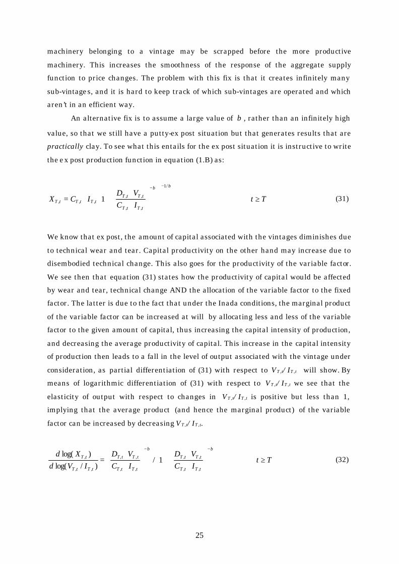
practically clay. To see what this entails for the ex post situation it is instructive to write

the ex post production function in equation (1.B) as:

TtICVD

ICXtTtT

tTtTtTtTtT ≥∀

⋅⋅

+⋅=

−− ββ /1

,,

,,,,, 1 (31)

We know that ex post, the amount of capital associated with the vintages diminishes due

to technical wear and tear. Capital productivity on the other hand may increase due to

disembodied technical change. This also goes for the productivity of the variable factor.

We see then that equation (31) states how the productivity of capital would be affected

by wear and tear, technical change AND the allocation of the variable factor to the fixed

factor. The latter is due to the fact that under the Inada conditions, the marginal product

of the variable factor can be increased at will by allocating less and less of the variable

factor to the given amount of capital, thus increasing the capital intensity of production,

and decreasing the average productivity of capital. This increase in the capital intensity

of production then leads to a fall in the level of output associated with the vintage under

consideration, as partial differentiation of (31) with respect to VT,t/IT,t will show. By

means of logarithmic differentiation of (31) with respect to VT,t/IT,t we see that the

elasticity of output with respect to changes in VT,t/IT,t is positive but less than 1,

implying that the average product (and hence the marginal product) of the variable

factor can be increased by decreasing VT,t/IT,t.

TtICVD

ICVD

IVdXd

tTtT

tTtT

tTtT

tTtT

tTtT

tT ≥∀

⋅⋅

+

⋅⋅

=−− ββ

,,

,,

,,

,,

,,

, 1/)/log(

)log( (32)

26

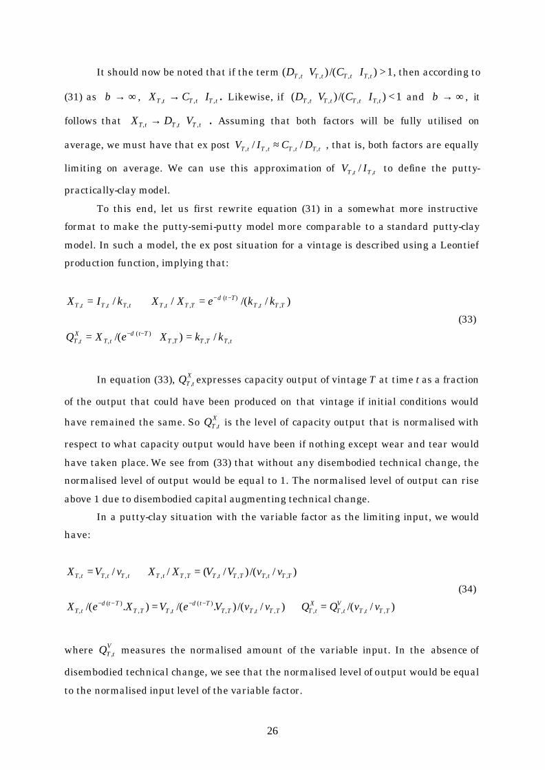
It should now be noted that if the term 1)/()( ,,,, >⋅⋅ tTtTtTtT ICVD , then according to

(31) as ∞→β , tTtTtT ICX ,,, ⋅→ . Likewise, if 1)/()( ,,,, <⋅⋅ tTtTtTtT ICVD and ∞→β , it

follows that tTtTtT VDX ,,, ⋅→ . Assuming that both factors will be fully utilised on

average, we must have that ex post tTtTtTtT DCIV ,,,, // ≈ , that is, both factors are equally

limiting on average. We can use this approximation of tTtT IV ,, / to define the putty-

practically-clay model.

To this end, let us first rewrite equation (31) in a somewhat more instructive

format to make the putty-semi-putty model more comparable to a standard putty-clay

model. In such a model, the ex post situation for a vintage is described using a Leontief

production function, implying that:

tTTTTTTt

tTX

tT

TTtTTt

TTtTtTtTtT

kkXeXQ

kkeXXkIX

,,,)(

,,

,,)(

,,,,,

/)/(

)//(//

=⋅=

⇒=⇒=

−⋅−

−⋅−

δ

δ

(33)

In equation (33), XtTQ , expresses capacity output of vintage T at time t as a fraction

of the output that could have been produced on that vintage if initial conditions would

have remained the same. So XtTQ , is the level of capacity output that is normalised with

respect to what capacity output would have been if nothing except wear and tear would

have taken place. We see from (33) that without any disembodied technical change, the

normalised level of output would be equal to 1. The normalised level of output can rise

above 1 due to disembodied capital augmenting technical change.

In a putty-clay situation with the variable factor as the limiting input, we would

have:

)//()//()./()./(

)//()/(//

,,,,,,,)(

,,)(

,

,,,,,,,,,

TTtTV

tTX

tTTTtTTTTt

tTTTTt

tT

TTtTTTtTTTtTtTtTtT

vvQQvvVeVXeX

vvVVXXvVX

=⇒=

⇒=⇒=

−−−− δδ

(34)

where VtTQ , measures the normalised amount of the variable input. In the absence of

disembodied technical change, we see that the normalised level of output would be equal

to the normalised input level of the variable factor.

27

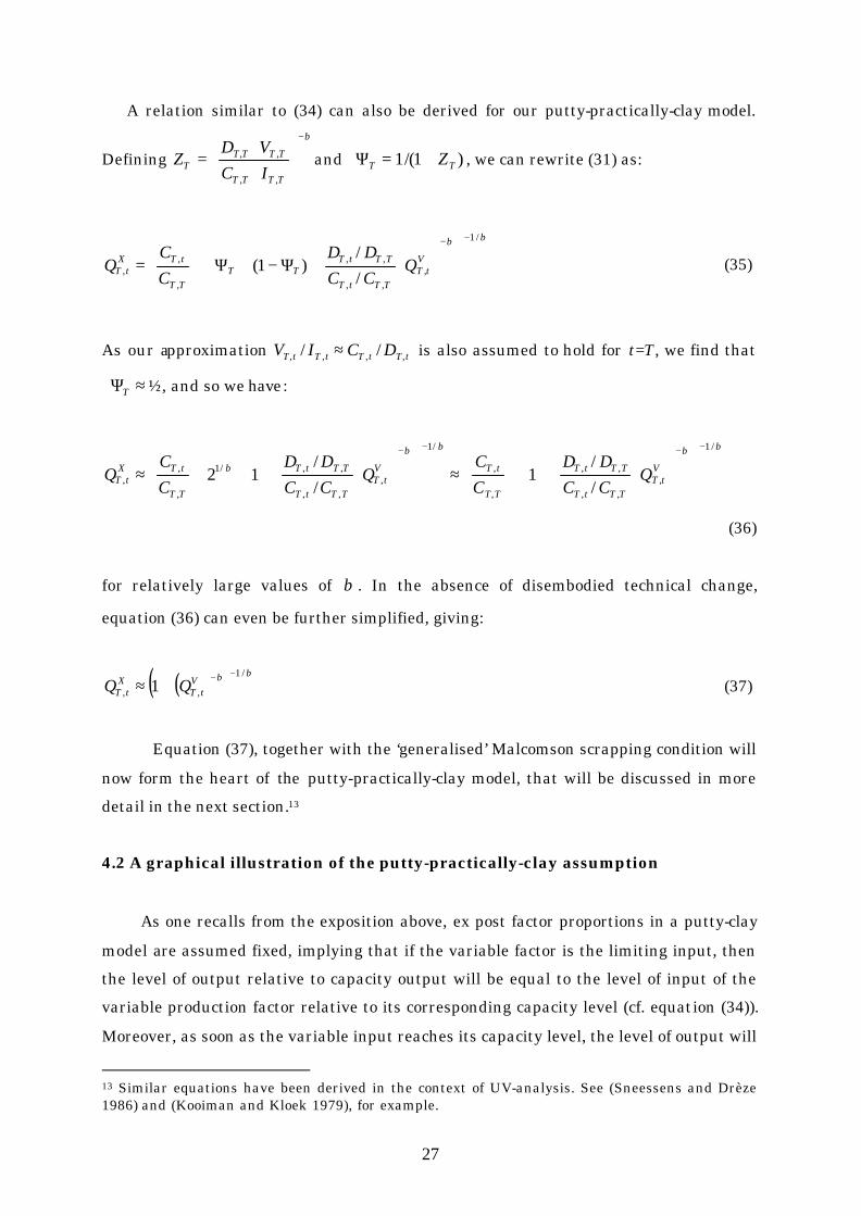
A relation similar to (34) can also be derived for our putty-practically-clay model.

Defining

β−

⋅⋅

=TTTT

TTTTT IC

VDZ

,,

,, and )1/(1 TT Z+=Ψ , we can rewrite (31) as:

ββ /1

,,,

,,

,

,, /

/)1(

−−

⋅⋅Ψ−+Ψ⋅

= V

tTTTtT

TTtTTT

TT

tTXtT Q

CCDD

CC

Q (35)

As our approximation tTtTtTtT DCIV ,,,, // ≈ is also assumed to hold for t=T, we find that

≈ΨT ½, and so we have:

ββββ

β

/1

,,,

,,

,

,

/1

,,,

,,/1

,

,, /

/1

//

12

−−−−

⋅+⋅

≈

⋅+⋅⋅

≈ V

tTTTtT

TTtT

TT

tTVtT

TTtT

TTtT

TT

tTXtT Q

CCDD

CC

QCCDD

CC

Q

(36)

for relatively large values of β . In the absence of disembodied technical change,

equation (36) can even be further simplified, giving:

( )( ) ββ /1

,, 1−−

+≈ VtT

XtT QQ (37)

Equation (37), together with the ‘generalised’ Malcomson scrapping condition will

now form the heart of the putty-practically-clay model, that will be discussed in more

detail in the next section.13

4.2 A graphical illustration of the putty-practically-clay assumption

As one recalls from the exposition above, ex post factor proportions in a putty-clay

model are assumed fixed, implying that if the variable factor is the limiting input, then

the level of output relative to capacity output will be equal to the level of input of the

variable production factor relative to its corresponding capacity level (cf. equation (34)).

Moreover, as soon as the variable input reaches its capacity level, the level of output will

13 Similar equations have been derived in the context of UV-analysis. See (Sneessens and Drèze 1986) and (Kooiman and Kloek 1979), for example.

28

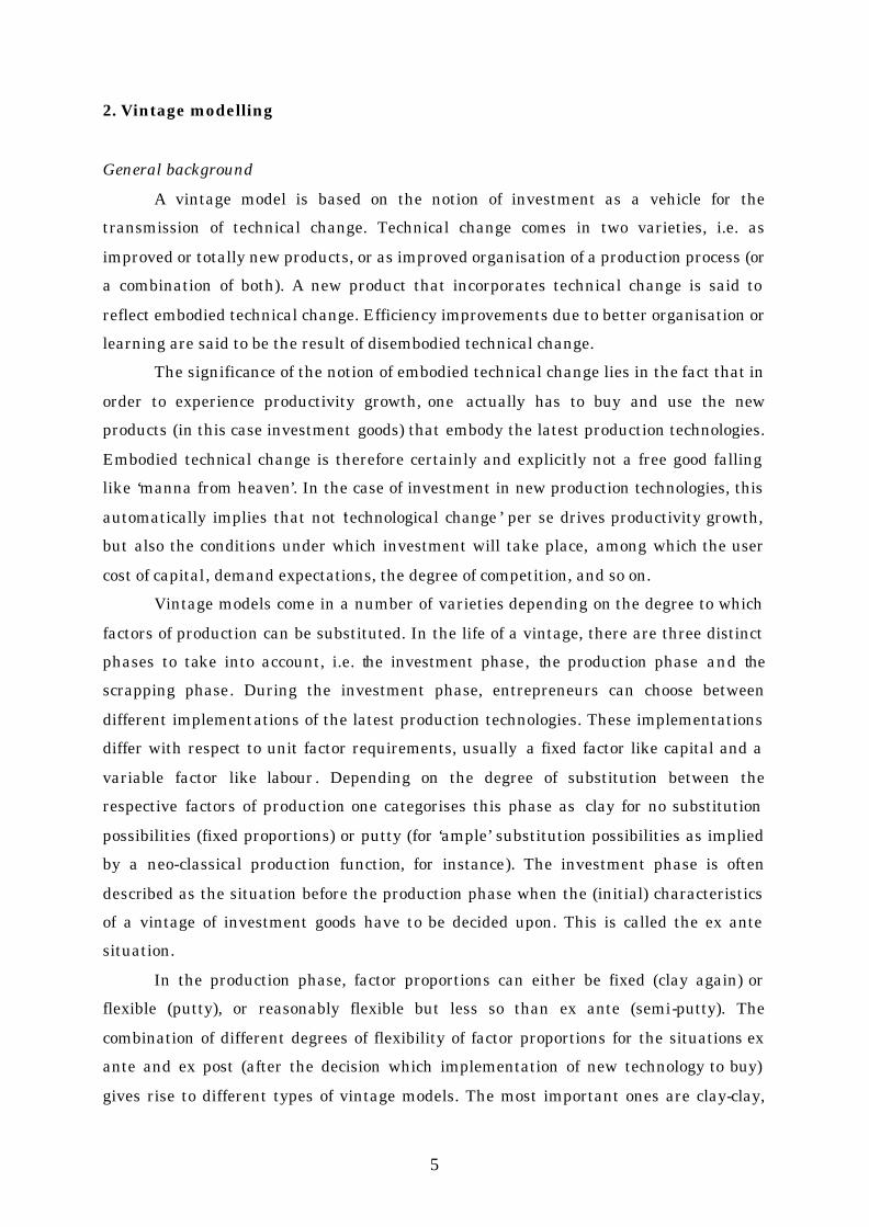
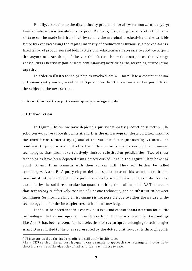
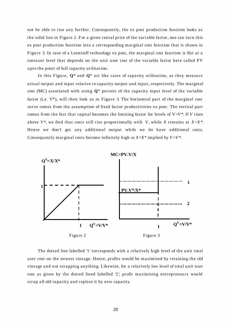
not be able to rise any further. Consequently, the ex post production function looks as

the solid line in Figure 2. For a given rental price of the variable factor, one can turn this

ex post production function into a corresponding marginal cost function that is shown in

Figure 3. In case of a Leontieff technology ex post, the marginal cost function is flat at a

constant level that depends on the unit user cost of the variable factor here called PV

upto the point of full capacity utilisation.

In this Figure, QX and QV act like rates of capacity utilisation, as they measure

actual output and input relative to capacity output and input, respectively. The marginal

cost (MC) associated with using QV percent of the capacity input level of the variable

factor (i.e. V*), will then look as in Figure 3. The horizontal part of the marginal cost

curve comes from the assumption of fixed factor productivities ex post. The vertical part

comes from the fact that capital becomes the limiting factor for levels of V>V*. If V rises

above V*, we find that costs still rise proportionally with V, while X remains at X=X*.

Hence we don’t get any additional output while we do have additional costs.

Consequently marginal costs become infinitely high at X=X* implied by V=V*.

Figure 2 Figure 3

The dotted line labelled ‘1’ corresponds with a relatively high level of the unit total

user cost on the newest vintage. Hence, profits would be maximised by retaining the old

vintage and not scrapping anything. Likewise, for a relatively low level of total unit user

cost as given by the dotted lined labelled ‘2’, profit maximising entrepreneurs would

scrap all old capacity and replace it by new capacity.

QV=V/V* 1

1

QX=X/X* MC=PV.V/X

PV.V*/X*

1

QV=V/V* 1

2

29

Obviously, for total unit costs close to PV.V*/X* a small change in PV may result in

the scrapping of an entire old vintage. Since in the putty-practically-clay case all old

capacity is contained in just one vintage, this may result in an infinitely high price

elasticity of total capacity. In order to avoid this, we may assume that there is some ‘fine -

structure’ within our old vintage, that would generate a concave ex post production

function that has the ex post production function from Figure 2 as a limiting case (i.e. as

an asymptote). Equation (37) will actually do the trick. For ever larger values of β , the

graph of equation (37) comes ever closer to the graph of the ex post production function

in Figure 2. This follows immediately from the fact that for a value of QV >= 1 and for

∞→β , we find 1→XQ , whereas for 0<QV<1 we find that the term 1 >>−βVQ , so

that VX QQ → in this case.

Using (37), the corresponding marginal cost function is given by:

βββ /)1(*

*** )1(

.)//(/)( ++⋅=

∂∂

⋅=∂∂

=∂∂

⋅= VV

XV Q

XVPV

VQQ

XPVVX

PVXV

PVQMC (38)

It should be noted that equation (38) only solves our problem for cases like those

represented by the horizontal dotted line labelled ‘1’ in Figure 3, i.e. for

MC>MC*=P*.V*/X*. For a case like the dotted line labelled ‘3’, we simply postulate that

the marginal cost function will be the mirror-image of (38), but then mirrored along the

vertical through QV=1/2 and the horizontal through MC*=P*.V*/X*. In that case we

would have for MC<MC*:

βββ /)1(*

*

)11(.

)( +−−⋅= VV QX

VPVQMC (39)

In equation (39), replacing QV in (38) by 1-QV takes care of the vertical symmetry

axis through QV=1/2. Changing the ‘+’ sign into a ‘-‘sign in (38) takes care of the

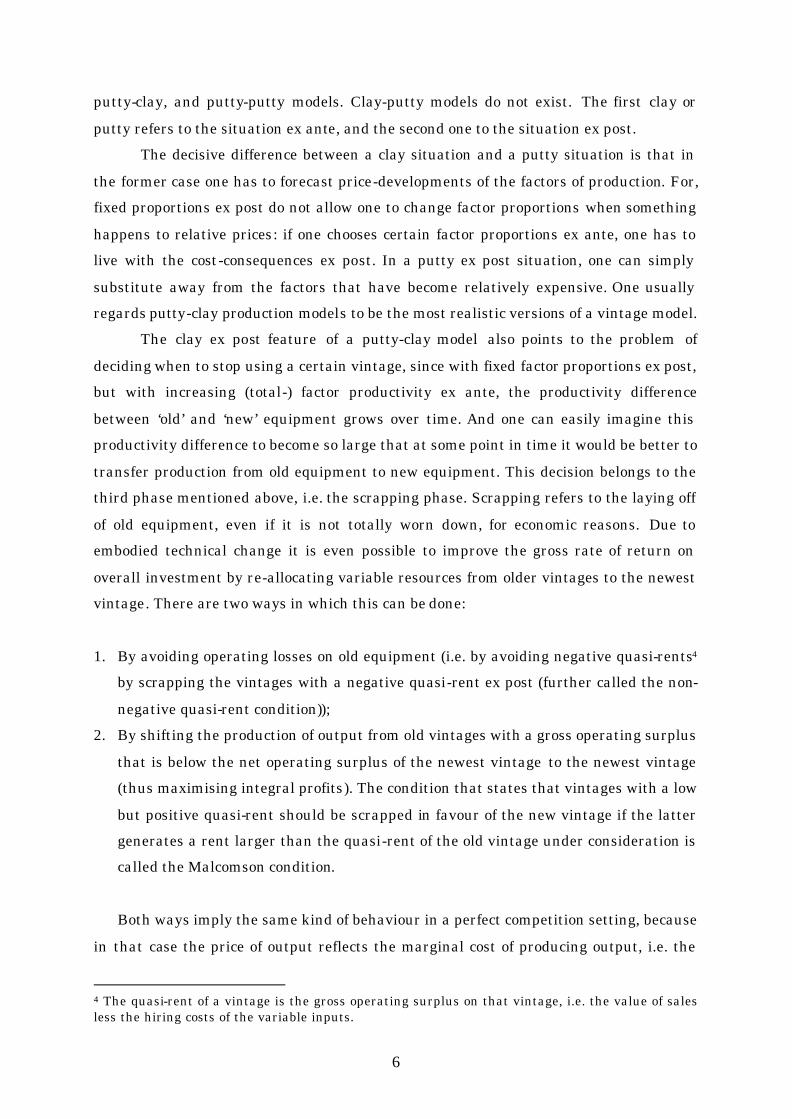
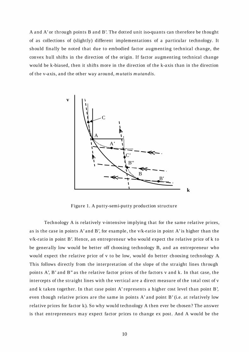
horizontal symmetry axis through MC=MC*.14 Thus, Figure 3 becomes Figure 4.

In Figure 3, the curved line (that looks like the graph of the tangent function) now

represents our ‘non-linearised’ ex post marginal cost function. The values of QV that we

can find for cases ‘1’ and ‘2’, for instance, will be taken to represent the survival fraction

of the old vintage, further denoted by sft, given the fairly bold assumption that we can

14 Note that the marginal cost function defined in this way is continuous in QV at QV=1/2.

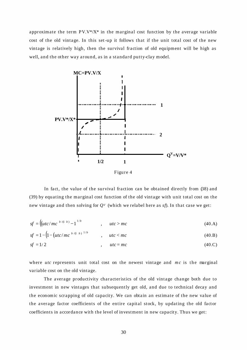
30

approximate the term PV.V*/X* in the marginal cost function by the average variable

cost of the old vintage. In this set-up it follows that if the unit total cost of the new

vintage is relatively high, then the survival fraction of old equipment will be high as

well, and the other way around, as in a standard putty-clay model.

Figure 4

In fact, the value of the survival fraction can be obtained directly from (38) and

(39) by equating the marginal cost function of the old vintage with unit total cost on the

new vintage and then solving for QV (which we relabel here as sf). In that case we get:

( )( ) mcutcmcutcsf >−= + ,1//1)1/( βββ (40.A)

( )( ) mcutcmcutcsf <−−= + ,/11/1)1/( βββ (40.B)

mcutcsf == ,2/1 (40.C)

where utc represents unit total cost on the newest vintage and mc is the marginal

variable cost on the old vintage.

The average productivity characteristics of the old vintage change both due to

investment in new vintages that subsequently get old, and due to technical decay and

the economic scrapping of old capacity. We can obtain an estimate of the new value of

the average factor coefficients of the entire capital stock, by updating the old factor

coefficients in accordance with the level of investment in new capacity. Thus we get:

MC=PV.V/X

PV.V*/X*

1

2

QV=V/V* 1 1/2

31

( )( ) tttittttt

itt

it XXfsfXXFXF /)1(// ,,111 ⋅+⋅−⋅⋅= −−− δ (41)

where itF represents the total consumption of the services of any factor used to produce

output. 15 Likewise, ittf , represents the marginal factor coefficient of factor i on the

newest vintage. Equation (41) shows how the average factor coefficients of total

production capacity are a weighted average of the coefficients of old capacity and of new

capacity. The bigger the volume share of new capacity in total capacity, i.e. the bigger

ttt XX /, , the faster the average factor coefficients will change through investment in

new capacity, ceteris paribus.16

With respect to total capacity output, we now have:

ttttt XXsfX ,1)1( +⋅⋅−= −δ (42)

Obviously, absolute factor use can be obtained directly by multiplying the average

factor coefficients (given by (41)) with the level of aggregate capacity output (given by

(42)). This also goes for the stock(s) of capital.

In the next section we will show how the putty-practically-clay model performs as

compared to a full putty-clay model.

5. Some illustrative simulations

In this section we will present some results based on simulations that we

performed with the putty-practically-clay model, further abbreviated to ‘ppc’-model, and

the full putty-clay model (abbreviated to ‘pcl’-model) with Malcomson-scrapping. We did

not estimate the parameters of these models, but rather calibrated the ex-post

substitution parameter of the ‘ppc’-model to generate roughly the same aggregate output

figures as the ‘pcl’-model, as well as the same trend in these figures. Note that only the

ex post parts of the models are different, and that the scrapping procedure present in the

full ‘pcl’-model is replaced by the survival fraction equation and the update-equations for

aggregate factor coefficients of the ‘ppc’-model. In the latter model, all scrapping is 15 Obviously, equation (41) can be used to obtain variable unit cost of the old vintage by lagging factor coefficients by one period and then multiplying the lagged factor coefficients by the current market price of the factor under consideration. 16 The inverse of this capacity share is a rough estimate of the economic lifetime of machinery and equipment.

32

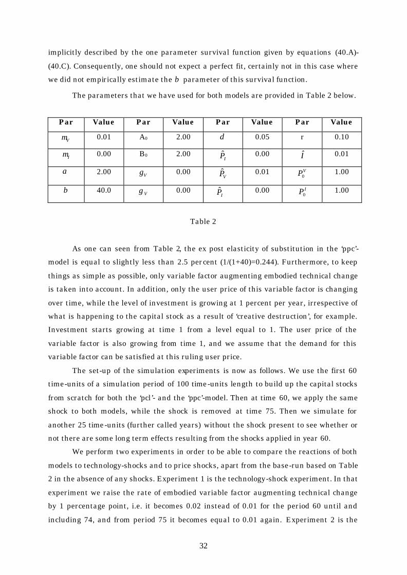
implicitly described by the one parameter survival function given by equations (40.A)-

(40.C). Consequently, one should not expect a perfect fit, certainly not in this case where

we did not empirically estimate the β parameter of this survival function.

The parameters that we have used for both models are provided in Table 2 below.

Par Value Par Value Par Value Par Value

Vµ 0.01 A0 2.00 δ 0.05 r 0.10

Iµ 0.00 B0 2.00 IP 0.00 I 0.01

α 2.00 Vγ 0.00 VP 0.01 VP0 1.00

β 40.0 Vγ 0.00 IP 0.00 IP0 1.00

Table 2

As one can seen from Table 2, the ex post elasticity of substitution in the ‘ppc’-

model is equal to slightly less than 2.5 percent (1/(1+40)=0.244). Furthermore, to keep

things as simple as possible, only variable factor augmenting embodied technical change

is taken into account. In addition, only the user price of this variable factor is changing

over time, while the level of investment is growing at 1 percent per year, irrespective of

what is happening to the capital stock as a result of ‘creative destruction’, for example.

Investment starts growing at time 1 from a level equal to 1. The user price of the

variable factor is also growing from time 1, and we assume that the demand for this

variable factor can be satisfied at this ruling user price.

The set-up of the simulation experiments is now as follows. We use the first 60

time-units of a simulation period of 100 time-units length to build up the capital stocks

from scratch for both the ‘pcl’- and the ‘ppc’-model. Then at time 60, we apply the same

shock to both models, while the shock is removed at time 75. Then we simulate for

another 25 time-units (further called years) without the shock present to see whether or

not there are some long term effects resulting from the shocks applied in year 60.

We perform two experiments in order to be able to compare the reactions of both

models to technology-shocks and to price shocks, apart from the base-run based on Table

2 in the absence of any shocks. Experiment 1 is the technology-shock experiment. In that

experiment we raise the rate of embodied variable factor augmenting technical change

by 1 percentage point, i.e. it becomes 0.02 instead of 0.01 for the period 60 until and

including 74, and from period 75 it becomes equal to 0.01 again. Experiment 2 is the

33

price-shock experiment. In that experiment we double the growth rate of the user-price

of the variable factor from a value of 0.01 to 0.02 and reduce the growth rate to 0.01

again from time 75.

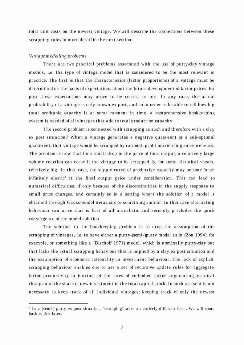
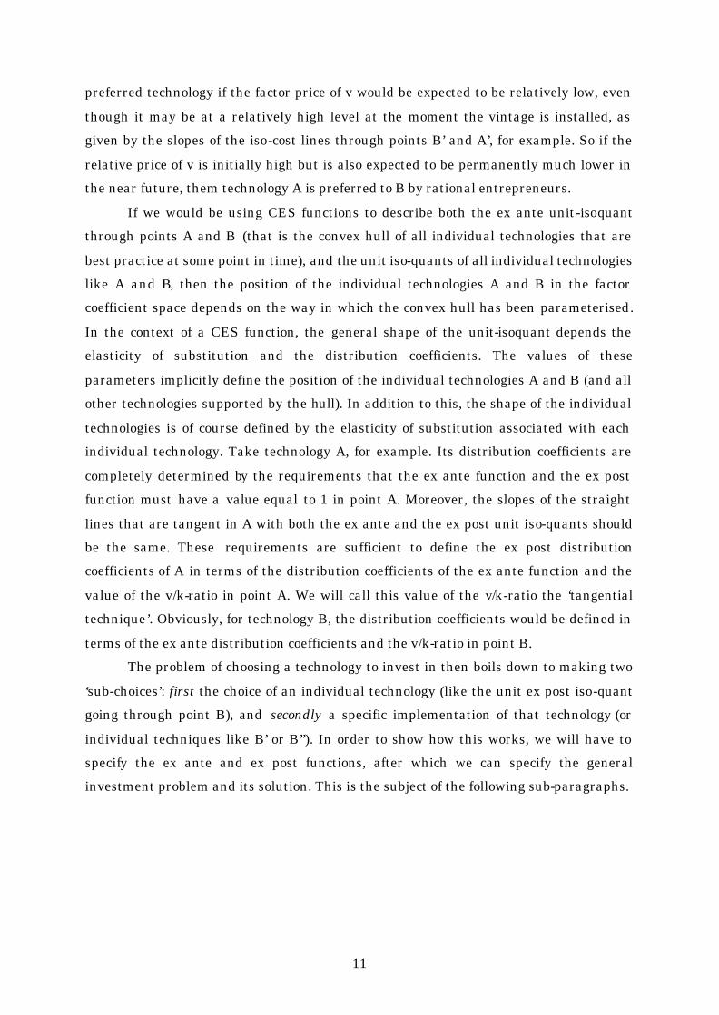
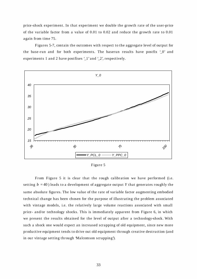
Figures 5-7, contain the outcomes with respect to the aggregate level of output for

the base-run and for both experiments. The baserun results have postfix ‘_0’ and

experiments 1 and 2 have postfixes ‘_1’ and ‘_2’, respectively.

Y_0

15

20

25

30

35

40

26 50 75 100

Y_PCL_0 Y_PPC_0

Figure 5

From Figure 5 it is clear that the rough calibration we have performed (i.e.

setting 40=β ) leads to a development of aggregate output Y that generates roughly the

same absolute figures. The low value of the rate of variable factor augmenting embodied

technical change has been chosen for the purpose of illustrating the problem associated

with vintage models, i.e. the relatively large volume reactions associated with small

price- and/or technology shocks. This is immediately apparent from Figure 6, in which

we present the results obtained for the level of output after a technology-shock. With

such a shock one would expect an increased scrapping of old equipment, since new more

productive equipment tends to drive out old equipment through creative destruction (and

in our vintage setting through ‘Malcomson scrapping’).

34

Y_1

0

5

10

15

20

25

30

35

40

45

50

26 50 75 100

Y_PCL_1 Y_PPC_1

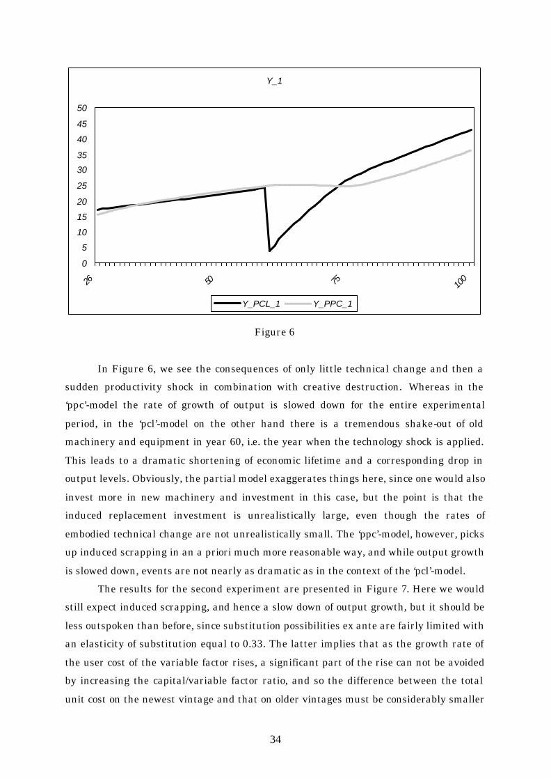
Figure 6

In Figure 6, we see the consequences of only little technical change and then a

sudden productivity shock in combination with creative destruction. Whereas in the

‘ppc’-model the rate of growth of output is slowed down for the entire experimental

period, in the ‘pcl’-model on the other hand there is a tremendous shake-out of old

machinery and equipment in year 60, i.e. the year when the technology shock is applied.

This leads to a dramatic shortening of economic lifetime and a corresponding drop in

output levels. Obviously, the partial model exaggerates things here, since one would also

invest more in new machinery and investment in this case, but the point is that the

induced replacement investment is unrealistically large, even though the rates of

embodied technical change are not unrealistically small. The ‘ppc’-model, however, picks

up induced scrapping in an a priori much more reasonable way, and while output growth

is slowed down, events are not nearly as dramatic as in the context of the ‘pcl’-model.

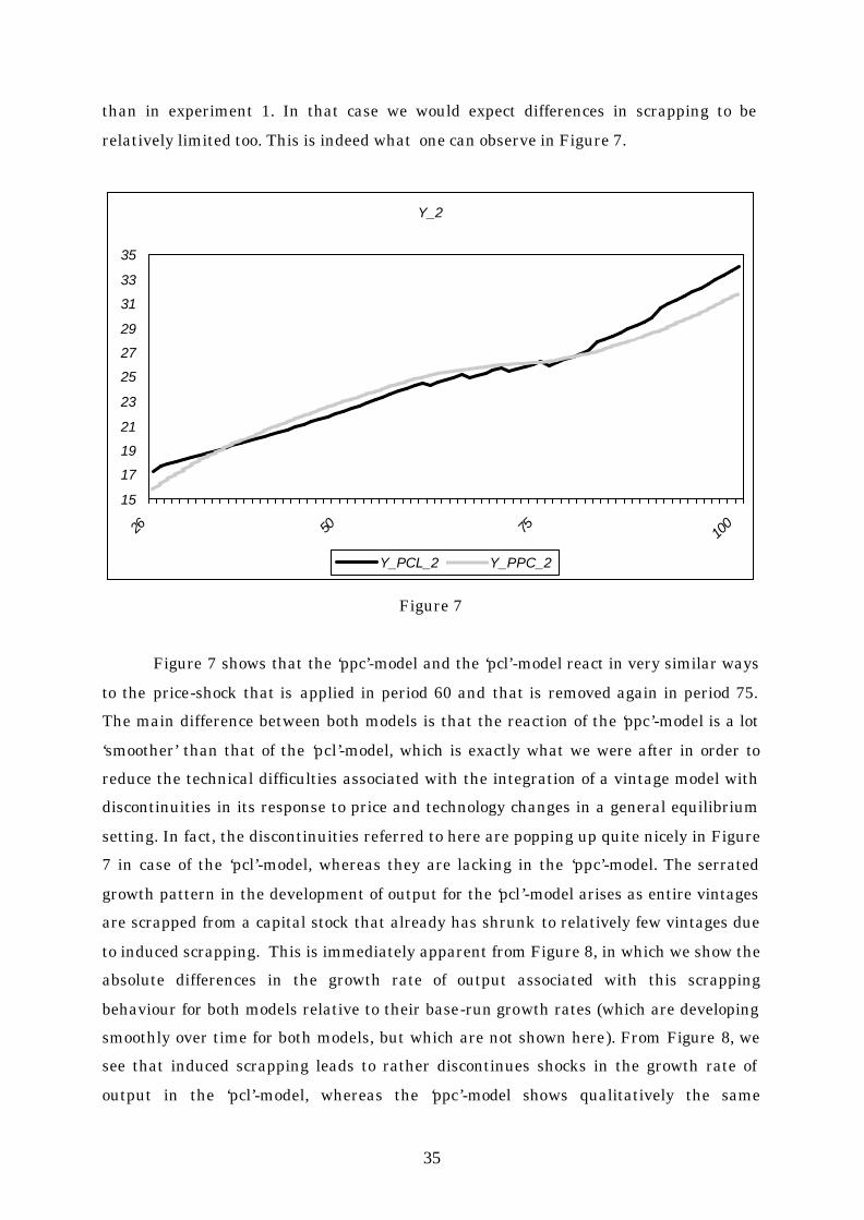
The results for the second experiment are presented in Figure 7. Here we would

still expect induced scrapping, and hence a slow down of output growth, but it should be

less outspoken than before, since substitution possibilities ex ante are fairly limited with

an elasticity of substitution equal to 0.33. The latter implies that as the growth rate of

the user cost of the variable factor rises, a significant part of the rise can not be avoided

by increasing the capital/variable factor ratio, and so the difference between the total

unit cost on the newest vintage and that on older vintages must be considerably smaller

35

than in experiment 1. In that case we would expect differences in scrapping to be

relatively limited too. This is indeed what one can observe in Figure 7.

Y_2

15

17

19

21

23

25

27

29

31

33

35

26 50 75 100

Y_PCL_2 Y_PPC_2

Figure 7

Figure 7 shows that the ‘ppc’-model and the ‘pcl’-model react in very similar ways

to the price-shock that is applied in period 60 and that is removed again in period 75.

The main difference between both models is that the reaction of the ‘ppc’-model is a lot

‘smoother’ than that of the ‘pcl’-model, which is exactly what we were after in order to

reduce the technical difficulties associated with the integration of a vintage model with

discontinuities in its response to price and technology changes in a general equilibrium

setting. In fact, the discontinuities referred to here are popping up quite nicely in Figure

7 in case of the ‘pcl’-model, whereas they are lacking in the ‘ppc’-model. The serrated

growth pattern in the development of output for the ‘pcl’-model arises as entire vintages

are scrapped from a capital stock that already has shrunk to relatively few vintages due

to induced scrapping. This is immediately apparent from Figure 8, in which we show the

absolute differences in the growth rate of output associated with this scrapping

behaviour for both models relative to their base-run growth rates (which are developing

smoothly over time for both models, but which are not shown here). From Figure 8, we

see that induced scrapping leads to rather discontinues shocks in the growth rate of

output in the ‘pcl’-model, whereas the ‘ppc’-model shows qualitatively the same

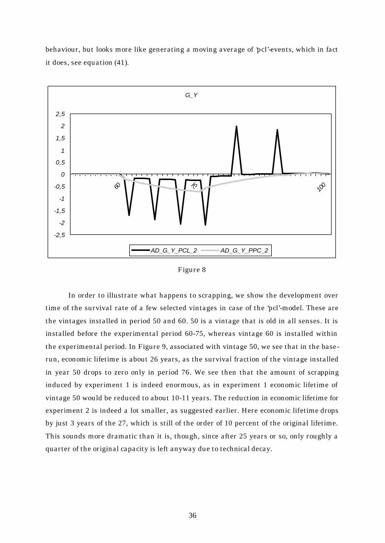
36

behaviour, but looks more like generating a moving average of ‘pcl’-events, which in fact

it does, see equation (41).

G_Y

-2,5

-2

-1,5

-1

-0,5

0

0,5

1

1,5

2

2,5

60 75 100

AD_G_Y_PCL_2 AD_G_Y_PPC_2

Figure 8

In order to illustrate what happens to scrapping, we show the development over

time of the survival rate of a few selected vintages in case of the ‘pcl’-model. These are

the vintages installed in period 50 and 60. 50 is a vintage that is old in all senses. It is

installed before the experimental period 60-75, whereas vintage 60 is installed within

the experimental period. In Figure 9, associated with vintage 50, we see that in the base-

run, economic lifetime is about 26 years, as the survival fraction of the vintage installed

in year 50 drops to zero only in period 76. We see then that the amount of scrapping

induced by experiment 1 is indeed enormous, as in experiment 1 economic lifetime of

vintage 50 would be reduced to about 10-11 years. The reduction in economic lifetime for

experiment 2 is indeed a lot smaller, as suggested earlier. Here economic lifetime drops

by just 3 years of the 27, which is still of the order of 10 percent of the original lifetime.

This sounds more dramatic than it is, though, since after 25 years or so, only roughly a

quarter of the original capacity is left anyway due to technical decay.

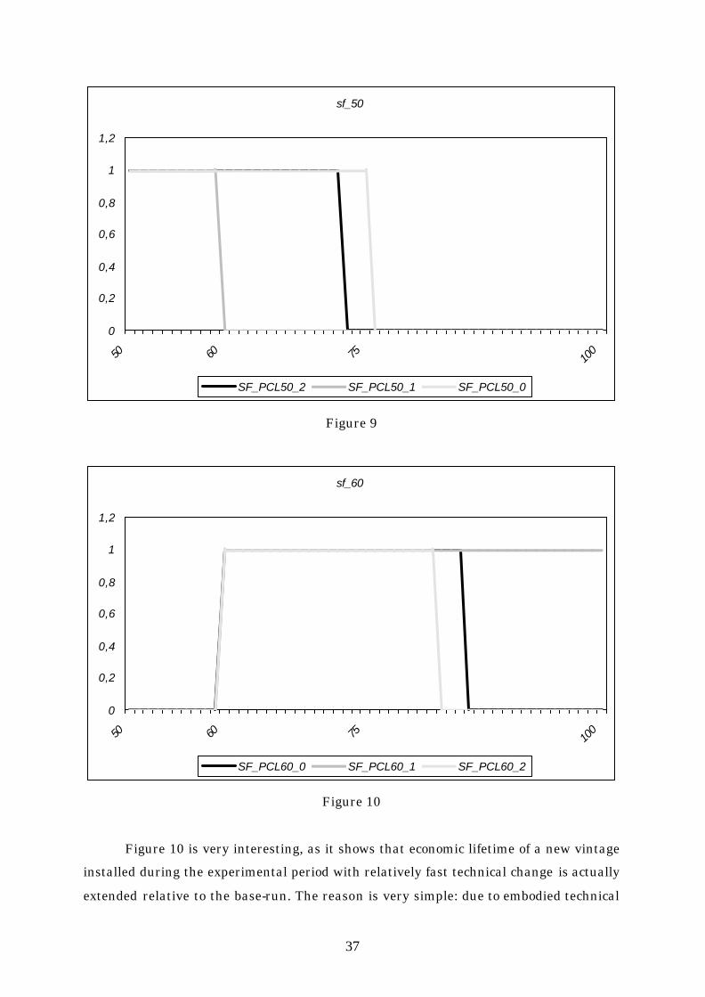
37

sf_50

0

0,2

0,4

0,6

0,8

1

1,2

50 60 75 100

SF_PCL50_2 SF_PCL50_1 SF_PCL50_0

Figure 9

sf_60

0

0,2

0,4

0,6

0,8

1

1,2

50 60 75 100

SF_PCL60_0 SF_PCL60_1 SF_PCL60_2

Figure 10

Figure 10 is very interesting, as it shows that economic lifetime of a new vintage

installed during the experimental period with relatively fast technical change is actually

extended relative to the base-run. The reason is very simple: due to embodied technical

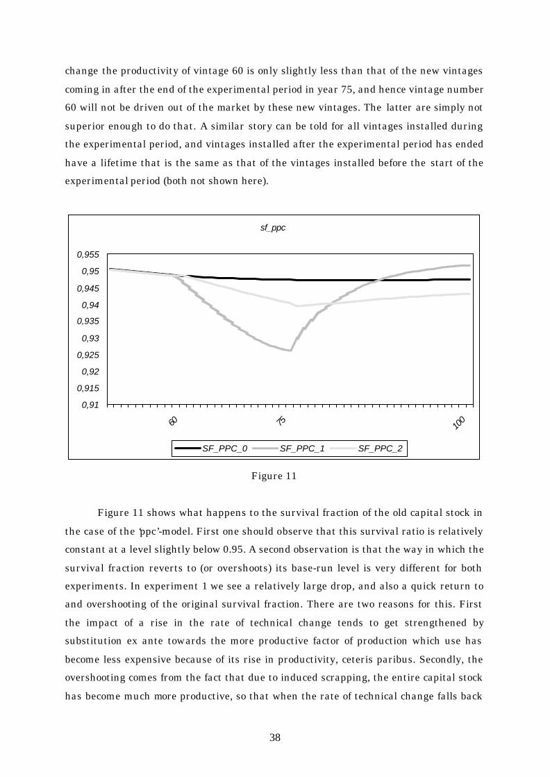
38

change the productivity of vintage 60 is only slightly less than that of the new vintages

coming in after the end of the experimental period in year 75, and hence vintage number

60 will not be driven out of the market by these new vintages. The latter are simply not

superior enough to do that. A similar story can be told for all vintages installed during

the experimental period, and vintages installed after the experimental period has ended

have a lifetime that is the same as that of the vintages installed before the start of the

experimental period (both not shown here).

sf_ppc

0,91

0,915

0,92

0,925

0,93

0,935

0,94

0,945

0,95

0,955

60 75 100

SF_PPC_0 SF_PPC_1 SF_PPC_2

Figure 11

Figure 11 shows what happens to the survival fraction of the old capital stock in

the case of the ‘ppc’-model. First one should observe that this survival ratio is relatively

constant at a level slightly below 0.95. A second observation is that the way in which the

survival fraction reverts to (or overshoots) its base-run level is very different for both

experiments. In experiment 1 we see a relatively large drop, and also a quick return to

and overshooting of the original survival fraction. There are two reasons for this. First

the impact of a rise in the rate of technical change tends to get strengthened by

substitution ex ante towards the more productive factor of production which use has

become less expensive because of its rise in productivity, ceteris paribus. Secondly, the

overshooting comes from the fact that due to induced scrapping, the entire capital stock

has become much more productive, so that when the rate of technical change falls back

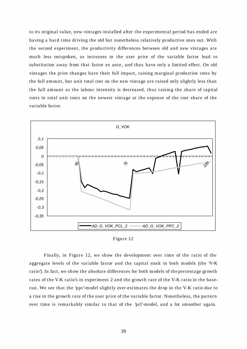
39

to its original value, new vintages installed after the experimental period has ended are

having a hard time driving the old but nonetheless relatively productive ones out. With

the second experiment, the productivity differences between old and new vintages are

much less outspoken, as increases in the user price of the variable factor lead to

substitution away from that factor ex ante, and thus have only a limited effect. On old

vintages the price changes have their full impact, raising marginal production costs by

the full amount, but unit total cost on the new vintage are raised only slightly less than

the full amount as the labour intensity is decreased, thus raising the share of capital

costs in total unit costs on the newest vintage at the expense of the cost share of the

variable factor.

G_VOK

-0,35

-0,3

-0,25

-0,2

-0,15

-0,1

-0,05

0

0,05

0,1

60 75 100

AD_G_VOK_PCL_2 AD_G_VOK_PPC_2

Figure 12

Finally, in Figure 12, we show the development over time of the ratio of the

aggregate levels of the variable factor and the capital stock in both models (the ‘V-K

ratio’). In fact, we show the absolute differences for both models of the percentage growth

rates of the V-K ratio’s in experiment 2 and the growth rate of the V-K ratio in the base-

run. We see that the ‘ppc’-model slightly over-estimates the drop in the V-K ratio due to

a rise in the growth rate of the user price of the variable factor. Nonetheless, the pattern

over time is remarkably similar to that of the ‘pcl’-model, and a lot smoother again.

40

Similar results are obtained for the other variables at the aggregate level (not shown

here).

6. Summary and concluding remarks

Technical change comes in two main varieties: organisation of the production

process, and improved machinery and equipment. Productivity improvements due to

improved quality of investment goods can obviously only be realised through new

investment. This has two main consequences for the rate of diffusion of technical change

at the aggregate level. First, the rate of diffusion is bounded by the share of new

investment in the total capital stock (only if that share equals 100%, then the rate of

technical change at the aggregate level is equal to that embodied in new investment).

Secondly, in general the existing capital stock represents a large amount of sunk costs,

but more importantly also ‘sunk productivity characteristics’. This implies that if these

productivity characteristics need to change, then the entire body of capital will need to

change as well through replacement investment at the margin of that same capital stock.

Hence, depending on the number of vintages contained by the capital stock, a noticeable

change of productivity characteristics at the aggregate level may take up both a lot of

time and a lot of resources (in the form of replacement investment). This is extremely

important in the face of the timing of policies geared at fundamentally changing the

productivity characteristics of the production process at the aggregate level, as is

foreseen to be necessary in order to avoid the consequences of global warming. So big

changes need a long time to be implemented in a clay-ex post setting, while the present

lack of consensus regarding the necessity of the Kyoto-protocol, in combination with the

surge in growth performance of countries like China and India, leaves less and less time

to accomplish these changes. This suggests that the actual timing of policy measures

becomes almost as crucial as the type of policy itself. It is for this reason, that putty-clay

models of production should be used to represent technology rather than aggregate

production functions, since the latter exaggerate substitution possibilities between

factors of production and consequently underestimate the volume of the resources and

the amount of time necessary to realise the changes in productivity characteristics

deemed necessary to achieve the Kyoto-targets. The adagio ‘better safe than sorry’, does

not only apply to the Kyoto-targets themselves, but also therefore to using a putty-clay

model of production rather than some neo-classical nested aggregate KLEM-production

function.

41

In this paper we have formulated a putty-semi-putty vintage model of production

based on CES ex ante and ex post production functions. The putty-semi-putty model

contains both the putty-clay model and the aggregate production function model as a

special case. We use the putty-semi-putty model to derive an equation for the ex post

utilisation level of capacity output on old vintages in function of the utilisation level of

the variable production factor(s) associated with those same old vintages. We interpret

this ex post level of the utilisation of capacity output as the survival fraction of old

equipment. Using this equation, it is possible to skip the usual administrative hassle

associated with a full putty-clay vintage model of production, by splitting the entire

vintage capital stock up into just two vintages: the first one consisting of new equipment

and the second one consisting of all old equipment. The productivity characteristics of

old equipment can then be obtained by updating them in function of the share of new

investment in the total capital stock, and the actual rate(s) of embodied technical

change.

Even though the putty-practically-clay model thus defined has been calibrated

only very roughly, we were able to show that it solves a number of difficulties associated

with the use of full putty-clay models in a wider general equilibrium modelling context.

First, the discontinuities of the scrapping induced by price and/or technology shocks in

the context of a full putty-clay model do not occur in the putty-practically-clay model.

Hence, the numerical difficulties associated with using a putty-clay model do not have to

arise when using the putty-practically-clay approach. Secondly, the putty-practically-

clay approach saves a lot of administrative hassle, since it distinguishes between just

two vintages consisting of new and old equipment. New equipment becoming old,

changes the productivity characteristics of old equipment in direct proportion with it’s

share in the capital stock.

Using some illustrative simulations, we were able to show that both the putty-

clay and the putty-practically-clay models generate qualitatively the same responses to

price and technology shocks, while the putty-practically-clay model also avoids the

occurrence of induced ‘daisy-cutter-scrapping’ that obliterates almost the entire capital

stock due to a shock in technology after a prolonged period of little progress. The latter

situation may be a relevant description of the current period where further efficiency

increases in traditional energy technologies are running out of gas, and the need to

develop alternative energy technologies becomes ever more pressing. If these needs are

translated into an equivalent increase in R&D resources devoted to finding such

alternatives, and if these R&D activities are successful, we will have the situation at

42

hand, where the actual diffusion of new technologies becomes a practical bottle-neck in

realising the productivity potential of new technology that may call for well timed policy-

action.

43

References

Aghion, P. a. P. H. (1992). "A Model of Growth through Creative Destruction." Econometrica 60: 323-51. Bischoff, C. W. (1971). The Effect of Alternative Lag Distributions. in: Tax Incentives and Capital Spending. G. F. (editor), The Brookings Institution, Washington D.C.: 61-130. Campbell, J.R. (1998), "Entry, Exit, Embodied Technology and Business Cycles", Review of Economic Dynamics, 1:371-408. Cooper, R., Haltiwanger J. and L. Power (1999), "Machine Replacement and the Business Cycle: Lumps and Bumps", American Economic Review, 89(4):921-946. Gilchrist, S. and J.C. Williams (2000), "Putty-Clay and Investment: A Business Cycle Analysis", Journal of Political Economy, 108(5):928-960. Greenwood, J., Hercowitz Z. and G.W. Huffman (1988), "Investment, Capacity Utilization and the Real Business Cycle", American Economic Review, 78(3):402-417. Grossman, G. M. and E. Helpman (1991). Innovation and Growth in the Global Economy, MIT Press, Cambridge Massachusetts. Hartog, H. den and H.S. Tjan (1974), Investeringen, lonen, prijzen en arbeidsplaatsen (Een jaargangenmodel met vaste coëfficiënten voor Nederland), Occasional Papers nr. 8, Centraal Planbureau. Italianer, A. (1984). The HERMES model: complete specification and first estimation results, report EUR 10669, Commission of the European Communities, DG XII. Jorgenson, D. and W. (1966). "The Embodiment Hypothesis." Journal of Political Economy 74(1): 1-17. Kooiman, P. a. T. K. (1979). " Aggragation of micro markets in disequilibrium: theory and application to the Dutch labour market, 1948-1975." Working Paper, Erasmus University Rotterdam. Malcomson, J. M. (1975). "Replacement and the Rental Value of Capital Equipment Subject to Obsolescense." Journal of Economic Theory Vol. 10: 24-41. Muysken, J. and A. H. v. Zon (1987). "Employment and Unemployment in the Netherlands, 1960-1984: A Putty-Clay Approach." Recgerches Economiques de Louvain 53(2): 101-133. Romer, P. (1990). "Endogenous Technological Change." Journal of Political Economy 98(5): S71-S102. Salter, W. (1960). Productivity and Technical Change, Cambridge University Press.

44

Solow, R. M. (1957). "Technical Change and the Aggregate Production Function." Review of Economics and Statistics Vol. 39: 312-330. Solow, R. M. (1960). Investment and Technical Progress. in: Mathematical Methods in the Social Sciences, 1959. S. K. K. Arrow and P. S. (eds.), Stanford University Press, Stanford CA: 89-104. Solow, R. M. (2000). Growth Theory: An Exposition, Oxford University Press, Oxford. Solow, R. M., Tobin, J., et al. (1966). "Neoclassical Growth with Fixed Factor Proportions." Review of Economic Studies Vol. 33: 79-115. Zon, A. H. v. (1991). "Vintage Capital and the Measurement of Technological Progress." in: Technology and Productivity; The Challenge for Economic Policy OECD, Paris: 171-185. Zon, A. H. v. (1994). RUM: a Simple Recursive Update Model Providing a condensed Representation of a Putty-Semi-Putty Vintage Model, MERIT, State university of Limburg, Maastricht.