Meridional variation in tropospheric methane on Titan

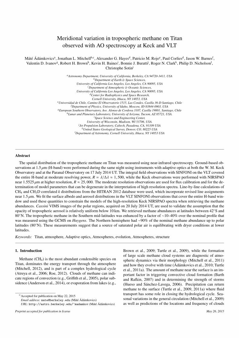
Meridional variation in tropospheric methane on Titanobserved with AO spectroscopy at Keck and VLT

Mate Adamkovicsa, Jonathan L. Mitchellb,c, Alexander G. Hayesd, Patricio M. Rojoe, Paul Corliesd, Jason W. Barnesf,Valentin D. Ivanovg, Robert H. Brownh, Kevin H. Bainesi, Bonnie J. Burattij, Roger N. Clarkk, Philip D. Nicholsonl,

Christophe Sotinj

aAstronomy Department, University of California, Berkeley, CA 94720-3411, USAbDepartment of Earth & Space Sciences,

University of California Los Angeles, Los Angeles, CA 90095, USAcDepartment of Atmospheric & Oceanic Sciences,

University of California Los Angeles, Los Angeles, CA 90095, USAdCenter for Radiophysics and Space Research,

Cornell University, Ithaca, NY 14853, USAeUniversidad de Chile, Camino El Observatorio 1515, Las Condes, Casilla 36-D Santiago, Chile

fDepartment of Physics, University of Idaho, Moscow, ID 83844-0903, USAgEuropean Southern Observatory, Ave. Alonso de Cordova 3107, Casilla 19001, Santiago, Chile

hLunar and Planetary Laboratory, University of Arizona, Tucson, AZ 85721, USA.iSpace Science and Engineering Center,

University of Wisconsin, Madison, WI 53706, USA.jJet Propulsion Laboratory, Caltech, Pasadena, CA, 91109 USA

kUnited States Geological Survey, Denver, CO, 80225 USAlDepartment of Astronomy, Cornell University, Ithaca, NY 14853 USA

Abstract

The spatial distribution of the tropospheric methane on Titan was measured using near-infrared spectroscopy. Ground-based ob-servations at 1.5 µm (H-band) were performed during the same night using instruments with adaptive optics at both the W. M. KeckObservatory and at the Paranal Observatory on 17 July 2014 UT. The integral field observations with SINFONI on the VLT coveredthe entire H-band at moderate resolving power, R = λ/∆λ ≈ 1, 500, while the Keck observations were performed with NIRSPAOnear 1.5525 µm at higher resolution, R ≈ 25, 000. The moderate resolution observations are used for flux calibration and for the de-termination of model parameters that can be degenerate in the interpretation of high resolution spectra. Line-by-line calculations ofCH4 and CH3D correlated k distributions from the HITRAN 2012 database were used, which incorporate revised line assignmentsnear 1.5 µm. We fit the surface albedo and aerosol distributions in the VLT SINFONI observations that cover the entire H-band win-dow and used these quantities to constrain the models of the high-resolution Keck NIRSPAO spectra when retrieving the methaneabundances. Cassini VIMS images of the polar regions, acquired on 20 July 2014 UT, are used to validate the assumption that theopacity of tropospheric aerosol is relatively uniform below 10 km. We retrieved methane abundances at latitudes between 42S and80N. The tropospheric methane in the Southern mid-latitudes was enhanced by a factor of ∼10–40% over the nominal profile thatwas measured using the GCMS on Huygens. The Northern hemisphere had ∼90% of the nominal methane abundance up to polarlatitudes (80N). These measurements suggest that a source of saturated polar air is equilibrating with dryer conditions at lowerlatitudes.

Keywords: Titan, atmosphere, Adaptive optics, Atmospheres, evolution, Atmospheres, structure

1. Introduction

Methane (CH4) is the most abundant condensible species onTitan, dominates the energy transport through the atmosphere(Mitchell, 2012), and is part of a complex hydrological cycle(Atreya et al., 2006; Roe, 2012). Clouds of methane can indi-cate regions of convection (e.g., Griffith et al., 2005), polar sub-sidence (Anderson et al., 2014), or evaporation from lakes (e.g.,

IAccepted for publication on May 22, 2015Email address: [email protected] (Mate Adamkovics)URL: http://astro.berkeley.edu/~madamkov (Mate Adamkovics)

Brown et al., 2009; Turtle et al., 2009), while the formationof large scale methane cloud systems are diagnostic of atmo-spheric dynamics via their morphology (Mitchell et al., 2011)and how they evolve with time (Adamkovics et al., 2010; Turtleet al., 2011a). The amount of methane near the surface is an im-portant factor in triggering convective cloud formation (Barthand Rafkin, 2007) and in determining the strength of storms(Hueso and Sanchez-Lavega, 2006). Precipitation can returnmethane to the surface (Turtle et al., 2009, 2011a) where fluidtransport has some role in closing the hydrological cycle. Sea-sonal variations in the general circulation (Mitchell et al., 2009)as well as predictions of the locations and frequency of clouds

Preprint accepted for publication in Icarus May 26, 2015

(Schneider et al., 2012) depend on the distribution of methanenear the surface, both in the regolith and the lower atmosphere.

Lakes and seas of liquid hydrocarbons (Stofan et al., 2007)provide both sinks and sources of methane on the surface. Thenorth pole contains by far the greatest extent of open liquidson Titan (Hayes et al., 2008; Lorenz et al., 2008; Sotin et al.,2012; Lorenz et al., 2014). The largest sea, Kraken Mare, ex-tends down to 55 N at its southernmost point. A few low-latitude lake candidates have been suggested, one near the equa-tor (Griffith et al., 2012b), and one at 40 S latitude (Vixie et al.,2014). The sole large lake in Titan’s south polar region isOntario Lacus (Turtle et al., 2009), although there are severalbasins that have been identified as potential ”paleo-seas” thatencompass a similar areal fraction to the northern seas (Hayeset al., 2011a).

Liquids presumably concentrate at the poles because theyare the coldest points on the surface and therefore cold-trapsfor volatiles. However, the polar clustering might also be re-lated to higher precipitation at the poles (Rodriguez et al., 2009;Brown et al., 2010; Rodriguez et al., 2011) relative to the dune-filled equatorial desert (Lorenz et al., 2006; Radebaugh et al.,2008; Le Gall et al., 2011; Rodriguez et al., 2014), which maybe caused by circulation (Rannou et al., 2006; Friedson et al.,2009). The lower elevations of the poles relative to equatorialregions may also play a role (Iess et al., 2010; Lorenz et al.,2013). The reason for the pronounced North-South asymme-try in lake coverage is unknown. Aharonson et al. (2009) citedMilankovic-like cycles in Titan’s orbital parameters as a pos-sible explanation, which is supported by simulations of Titan’spaleoclimate (Lora et al., 2014).

The physical properties of lakes are complicated by the factthat they are likely mixtures of hydrocarbons. Though methanecomposes Titan’s raindrops, the seas may build up significantfractions of less-volatile ethane. Spectroscopic observations ofOntario Lacus suggest the presence of ethane (Brown et al.,2008), although the abundance is not constrained by these mea-surements. Recent observations of Ligeia Mare, conducted bythe Cassini RADAR instrument, have demonstrated that it isprimarily composed of methane (Mastrogiuseppe et al., 2014).Evaporation rates from a lake that is mostly methane will bemuch greater than from a lake that is mostly ethane (Mitri et al.,2007; Tokano, 2009). Lorenz (2014) points out that the ratio ofmethane to ethane may vary across lakes due to the concentra-tion of solutes by heterogeneous evaporation and dilution byheterogeneous rainfall.

While shoreline recession at Ontario Lacus was reported overthe timescale of the Cassini mission (Turtle et al., 2011b; Hayeset al., 2011b,a), the shoreline detection algorithms have beendisputed (Cornet et al., 2012), leaving the contemporary evap-oration rate over lakes uncertain. Cassini has observed albedovariations with both the Imaging Science Subsystem (ISS) andRADAR that depict smaller southern lakes disappearing be-tween adjacent observations (Turtle et al., 2009; Hayes et al.,2011a), which was attributed to either infiltration or evapora-tion, although the rates could not be quantified. Changes in lakeand sea volumes over geologic timescales have also likely oc-curred, as evidenced by the geomorphology of empty lakebeds

in some polar terrains and the presence of drowned river val-leys in the northern seas, which indicate that the liquid levelis rising faster than fluvial sediment is being deposited (Hayeset al., 2008). Some of the lakebeds show a bright reflection near5 µm, which is interpreted as a compositional signature that isattributed to the formation of organic evaporite (Barnes et al.,2011). The largest outcrop of evaporites are in the tropics, im-plying that these areas may have been seas during the geologi-cal past, perhaps under a different climatic regime (Moore andHoward, 2010; MacKenzie et al., 2014).

The evaporation of methane from surface lakes may havean observational impact on the atmosphere. Tokano (2014)recently revisited the Cassini radio occultation data (recordedfrom 2005–2009) and points out that retrievals assuming a uni-form tropospheric methane distribution lead to surface pressuredistributions that are inconsistent with the predictions of cir-culation models. Instead, Tokano (2014) argues for a substan-tially higher methane abundance in the Summer hemisphere.Penteado and Griffith (2010) searched for spatial variation inthe methane abundance with high resolution Keck observations.The unsaturated lines of the resolved 3ν2 band of CH3D aresensitive to possible changes in the tropospheric methane abun-dance. Their measurements from December 2006 indicated thatmethane below 10 km altitude is constant to within 20% in thetropical atmosphere, sampled between the range of 32S–18N.High resolution analysis with new methane lines lists (de Berghet al., 2012) illustrates that significant improvements can bemade in spectral fitting with recent laboratory data.

Here we present ground-based observations of the methanedistribution on Titan using a methodology that improve uponthe observing protocol and integration times of Penteado andGriffith (2010), and which are supported by both integralfield observations from the same night, as well as a Cassiniflyby from four days later. Our radiative transfer models in-clude revised methane line lists from the most recent HITRANdatabase. The observations, data reduction, and calibrations aredescribed in Section 2, while the radiative transfer model is de-tailed in Section 3. Results are presented in Section 4 and dis-cussed in Section 5.

2. Observations

Observations were performed on 17 July 2014 UT at both theParanal Observatory and the W. M. Keck Observatory. Instru-mentation with complementary observing modes, resolutions,and bandpasses provided flux calibration and characterizationof the physical properties of the atmosphere and surface. Fig-ure 1 illustrates the viewing geometry of the observations thatare described below.

2.1. VLT Observations

The Spectrograph for INtegral Field Observations in the NearInfrared (SINFONI) on the Very Large Telescope (VLT) atParanal Observatory was used as part of a campaign to mon-itor clouds on Titan. The spectrometer is fed by an adaptiveoptics module and uses two sets of stacked mirrors to optically

2

Keck NIRSPAO: 1.413 - 1.808 (um) 2014-07-17 UT

lat⊕, lon⊕=21.1N, 307Wlat¯, lon¯=22.6N, 301W

40N

20N

E

20S

VLT SINFONI: 1.577 - 1.597 (um) Cassini VIMS: 1.552 (um)

0.000

0.015

0.030

0.045

0.060

0.075

0.090

0.105

0.120

0.135

surf

ace

reflect

ance

(I/F)

0.000

0.015

0.030

0.045

0.060

0.075

0.090

0.105

0.120

reflect

ance

(I/F)

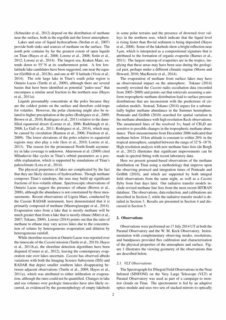
Figure 1: Viewing geometry and surface albedo of Titan during observations.An H-band image from the NIRSPAO slit viewing camera (top left) during thespectrometer exposures identifies the spatial location of the spectra. The widebandpass results in sensitivity to the atmospheric haze. An image from theSINFONI data cube (bottom left) that is sensitive to surface albedo variationsis shown with a white box that indicates the region of pixels that corresponds tothe NIRSPAO slit. This is the region considered when referring to pixels alongthe SINFONI “slit”. An orthographic reprojection of a 1.552 µm Cassini Visualand Infrared Mapping Spectrometer (VIMS) map, sampled at the SINFONIplate scale and artificially limb-darkened, illustrates the surface reflectance inthe absence of the atmospheric contribution and confirms the photometry andflux calibration of the SINFONI data (bottom right). The viewing geometry ofthe observations is show in the schematic (top right) with a grid spacing of 20degrees.

divide and rearrange the field of view (FOV) into a single syn-thetic long slit that is spectrally dispersed by a grating ontothe detector. We used the 0.8”×0.8” FOV, corresponding to aspatial pixel scale of 0.0125”×0.0250”, with the grating thatcovers 1.45 – 2.45 µm at a spectral resolution of ∆λ ≈ 1 nm,corresponding to a resolving power, R = λ/∆λ ≈ 1500 (Eisen-hauer et al., 2003). Four overlapping exposures with 2 × 15 seccoadds, offset by ±0.1” from the disk center in both the X andY directions of the FOV, are mosaicked to cover the entire disk.

Observations were reduced using version 2.5.2 of the SIN-FONI pipeline. The standard processing of the raw exposuresincludes correction of bad pixels, flat fielding, and correction ofgeometric distortions. The pipeline performs wavelength cali-bration and then reconstructs the 32 slices of spectra into a datacube. Sky frames are used to correct for sky emission.

The B3V type star Hip 74680 (HD 134485) was observedat an airmass of 1.019 and is used for both telluric correctionand flux calibration. A high resolution H-band telluric templatefrom ESO is convolved to the instrument resolution and scaledto fit telluric absorption features observed in the calibration starnear 1.47 and 1.58 µm; the normalized telluric template wasscaled by a factor of 0.7 (and offset by 0.3), and then used tocorrect the target spectra.

Photometric calibration was performed by integrating the

calibration star spectrum over the 2MASS filter curves in H-band and comparing with the known apparent magnitude. Therelative spectral response RH(λ), was used to determine the ob-served isoflux,

IH =

∫RH(λ)Iobs(λ)dλ∫

RH(λ)dλ, (1)

where Iobs(λ) is the observed spectrum. The 2MASS “zero-magnitude” reference flux in H-band from Cohen et al. (2003)is

Iref = 1.133 × 10−13 ± 2.212 × 10−15 W cm−2 µm−1.

The spectral bandpass of SINFONI covers all of H-band, in-cluding the entire 2MASS H-band filter range, which facilitatesthe calibration of the NIRSPAO observations that cover a nar-row band-pass at higher resolving power.

The apparent H-band magnitude of the calibrator is mH =

8.322 from 2MASS (Cutri et al., 2003), and the correction fac-tor for converting the observed photon count rate (DN/s) to fluxis given by

cH =Iref

IH10−mH/2.5. (2)

The photometrically calibrated spectra, I(λ) = Iobs(λ)cH, werethen converted to units of reflectivity,

IF

=r2

Ω

I(λ)F(λ)

, (3)

where r is the heliocentric distance to Titan, Ω is the solid an-gle (in steradians) of each spatial pixel, and πF(λ) is the solarspectrum at 1 AU, for which the 2000 ASTM Standard Extrater-restrial Spectrum Reference1 was used.

2.2. Keck ObservationsThe Near-InfraRed SPECctrometer (NIRSPEC) on the

Keck II telescope at W. M. Keck Observatory (McLean et al.,1998) was used with the adaptive optics (AO) system, NIR-SPEC+AO (NIRSPAO), for high resolution spectroscopy of Ti-tan with a pixel scale of 0.018”/pixel along the slit. The in-strument was setup in the cross-dispersed echelle mode in H-band with a 0.041”×2.26” slit, giving a resolving power ofR ≈ 25, 000. The echelle and cross-disperser angles were setto 62.8 and 36.5, respectively, nearly continuously covering therange 1.481 – 1.701 µm in 7 echelle orders. The edges of neigh-boring orders can overlap with the 2.26” slit in this setting.For this work we focused on Order 49, sampling the 1.541 –1.563 µm region, and where there was significant overlap at theedges of the order.

The standard ABBA dither (nod) pattern for the instrumentmoves the target 25% of the length of the slit (0.57”) from cen-ter, which would position the limb of the ∼0.8” disk of Titannear the overlapping region of echelle order. This was avoidedby using a smaller dither step along the slit. Sky exposures

1http://rredc.nrel.gov/solar/spectra/am0/

3

Table 1: Log of observations on 2014-07-17

Target Instrument Time (UTC) Exposure (s) Airmass Lon.a

Titan NIRSPAO 05:49:30 300 1.212 290.6Titan NIRSPAO 05:55:33 300 1.214 290.7Titan NIRSPAO 06:00:47 300 1.216 290.7Titan NIRSPAO 06:07:56 300 1.220 290.9Titan NIRSPAO 06:16:28 300 1.227 291.0Titan NIRSPAO 06:23:20 300 1.234 291.1Titan NIRSPAO 06:28:34 300 1.240 291.2Titan NIRSPAO 06:34:13 300 1.248 291.3Titan NIRSPAO 06:40:19 300 1.257 291.4Hip 77516 NIRSPAO 08:30:03 20 1.254 –Titan SINFONI 23:39:31 30 1.018 307.3Titan SINFONI 23:40:32 30 1.018 307.4Titan SINFONI 23:41:31 30 1.018 307.4Titan SINFONI 23:42:29 30 1.018 307.4Hip 74680 SINFONI 23:53:21 4 1.019 –

a Sub-observer longitude from JPL Horizons ephemerides.

taken completely off target were recorded for sky subtraction.The integration time for each spectrum was 300 s. Two ABBAsets were record with the slit aligned North-South near the cen-tral meridian, and one exposure was taken with Titan in thecenter of the slit, for a total of 2,700 s integration on target,followed by a 300 s sky exposure. The spectral type A0V cal-ibrator star was HD 141513 (Hip 77516). The logs for bothSINFONI and NIRSPAO observations are presented in Table 1.

The NIRSPAO data are reduced using standard proceduresfor bad pixel correction, flat fielding, and cosmic ray rejection.The spatial and spectral rectification routines from the RED-SPEC package are used before shifting and stacking exposures.A bare sky exposure is used for first order sky subtraction. Asecond order correction was performed by (1) offsetting eachexposure to the median of the stacked set near the edge of theorder, and then (2) scaling each exposure to the median valueat the center of the order. The stack of images for individualexposures was collapsed using the mean of each pixel.

Flux calibration of an extended object in a slit spectrome-ter can be challenging because the slit losses due to the pointspread function (PSF) extending over the edge of the slit needto be determined. For point sources, it can often be assumedthat the unknown slit losses for the calibrator and the targetare the same. However, this is not the case when comparinga point source calibrator and an extended target. After an ini-tial telluric and flux calibration was performed using Hip 77516(HD 141513), the NIRSPAO data were then scaled to match thecalibrated SINFONI observations. Two wavelengths were con-sidered that are sensitive to the surface and lower atmosphere,Figure 2.

Unlike the narrow NIRSPAO channels, which can probe re-gions of high methane opacities near 1.55 µm and therefore theatmosphere, the SINFONI channels near 1.55 µm are broad,cover regions of predominantly low methane opacity, and aretherefore more sensitive to the surface. Due to the difference inbandpass, the reflectance along the NIRSPAO slit at 1.5555 µm

20406080100120

pixel along slit

0.00

0.02

0.04

0.06

0.08

0.10

0.12

0.14

reflect

ance

(I/F)

South North

NIRSPAO

SINFONI

λ (µm)

1.5581

1.5585

1.5547

1.5550

1.5555

1.6145

Figure 2: Reflectance profiles along the NIRSPAO slit (black) and corre-sponding SINFONI pixels (red) at wavelengths that are sensitive to the surface(dashed), and atmosphere (dotted and solid). The profiles that are sensitive tothe surface are limb-darkened whereas the profiles sensitive to the atmosphereexhibit limb-brightening. The spatial region of pixels that is used from theSINFONI cube is illustrated by the white box in the bottom left panel of Fig-ure 1. The SINFONI pixel scale has been linearly mapped to the NIRSPAOpixel scale. The difference between reflectivity profiles of the surface (red andblack dashed curves) is consistent with the surface albedo changing due to therotation between the time of the two observations.

does not match the corresponding SINFONI channel and iscompared to the 1.6145 µm SINFONI channel in Figure 2. The1.55 µm spectral region is generally thought to be a surface-sensitive on Titan, however, when sampled at high spectral res-olution there are wavelengths in this region with large gas opac-ity that probe only the atmosphere.

2.3. Cassini VIMS ObservationsSpectral mapping cubes were obtained by Cassini VIMS

(Brown et al., 2004) during both the ingress and egress of the

4

T103 flyby on 2014 Jul 20 UT, and provide views of both po-lar regions. We reduce the VIMS IR channels from two cubes(datasets 1784502376 1 and 1784584782 1) using the standardpipeline for calibration and determination of the viewing ge-ometry. Images from the 1.573 µm and 1.625 µm channels areused to evaluate meridional variation in near-surface hazes to-ward both poles. Since the tropospheric haze opacity near thesurface can be degenerate with the methane abundance there(described below) we use the VIMS observations to differenti-ate between models.

3. Radiative Transfer

We implement a model of the atmosphere using the in situmeasurements made with instruments on the Huygens probe,which provide structure, chemical composition, and aerosolscattering in our reference model. Methane line assignmentsfrom the HITRAN 2012 database (Rothman et al., 2013) areused to determine gas opacities via line-by-line methods and wesolve the radiative transfer using the discrete ordinates method(Stamnes et al., 1988).

3.1. Structure and Composition

We use a model with 20 layers, which have boundaries(levels) that are evenly spaced in pressure above and below300 mbar (hPa), covering the 2.75 – 1466.45 mbar range sam-pled by the Huygens Atmospheric Structure Instrument (HASI)on Cassini (Fulchignoni et al., 2005). This corresponds to analtitude range from the surface up to 147 km. There are 10layers sampled at ∼30 mbar intervals through the tropopauseand stratosphere and 10 layers sampling the troposphere at∼115 mbar steps. Fewer layers can improve the computationalspeed, but yield inconsistent calculations, whereas increasingthe number of layers above 20 has no significant benefit. Alti-tude sensitivity for cloud retrievals may be improved with ad-ditional layers, but this topic is beyond the scope of this work.After the levels in the model are determined, the pressures, tem-peratures and densities for each layer are interpolated and thetotal column densities are determined using the mole fractionsreported by the Huygens Gas Chromatograph Mass Spectrome-ter (GCMS) (Niemann et al., 2010). The atmospheric structureand composition are tabulated in Table 2.

3.2. Aerosol Model

The aerosol scattering phase functions and opacities weremeasured in situ by the the Descent Imager-Spectral Radiome-ter (DISR) on the Huygens probe (Tomasko et al., 2008). Wefit 32nd order Legendre polynomials to the phase functions tab-ulated at 1.29 µm, 1.58 µm, and 2.00 µm, using a Levenberg-Marquardt (LM) optimization, and linearly interpolate coeffi-cients for intermediate wavelengths. The vertical opacity struc-ture from the model of (Tomasko et al., 2008) is used, with ahaze single scattering albedo, ωH = 0.96.

3.3. CH4 and CH3D opacitiesSpectra resolving the natural line shape of CH4 and CH3D

are calculated using line-by-line methods. These spectra areused to calculate correlated-k coefficients at the resolution anddispersion plate scale of both the NIRSPAO and SINFONI in-struments. Correlated-k values (Lacis and Oinas, 1991) for CH4and CH3D are calculated for 390 combinations of temperatureand pressure that have been used in the literature, e.g., by Sro-movsky et al. (2012) and Irwin et al. (2014). CH4 and CH3Dlines are from the HITRAN 2012 database (Rothman et al.,2013), which include the WKMC-80K methane line data ofCampargue et al. (2012) that are relevant to this spectral region.

We calculate the monochromatic opacity at frequency, ν,pressure P, and temperature, T , by summing over lines, `, asdescribed by Sromovsky et al. (2012),

k(ν; P,T ) =∑`

S `(T0) exp[

hcE`kB

(1

T0−

1T

)]Q(T0)Q(T )

f`(ν − ν`; P,T ), (4)

correcting the typo of the reversed T0 and T in the square brack-ets of their Equation 1. S `(T0) is the line strength at refer-ence temperature T0, E` is the lower state energy of the line,and the partition function ratio Q(T0)/Q(T ) is approximated by(T0/T )3/2. The speed of light, Planck and Boltzmann constantsare c, h, and kB, respectively.

The line shape function, f`, is given by the Voigt profile witha correction to the Lorentz far wing, χ(ν − ν0).

f`(ν − ν0; P,T ) = V(ν0;αD, αL) χ(ν − ν0) (5)

where∫ ∞

−∞

f`(ν) dν = 1 (6)

Various prescriptions for χ are in the literature and we use thesub-Lorenztian line shape of Campargue et al. (2012) that is de-termined from laboratory data. The following notation is usedto describe the Voigt profile when determining line shape:

V(x;σ, γ) =

∫ ∞

−∞

G(x′;σ)L(x − x′; γ)dx′ (7)

where

G(x;σ) ≡e−x2/(2σ2)

σ√

2πand L(x; γ) ≡

γ

π(x2 + γ2). (8)

The integral in Equation 7 can be evaluated with the real partof the complex error function. The Voigt line shape in terms ofphysical parameters is given by:

V(ν0;αD, αL) = V(σ, γ)

√ln(2)π

αD (9)

where the dimensionless parameters

σ =ν − ν0

αD

√ln(2) and γ =

αL

αD

√ln(2) (10)

are given in terms of the following physical parameters

αD =ν0

c

√2kTm

and αL = γairPP0

(T0

T

)n

(11)

5

Table 2: Atmospheric Structurea and Compositionb

Layer Pressure Altitude Temperature Density Total Column CH4 Column(mbar) (km) (K) (cm−3) (cm−2) (km amg) (km amg)

1 9.5 105.8 121.1 5.75e+17 5.14e+24 1.91 0.02862 44.9 59.1 79.1 4.13e+18 4.89e+24 1.82 0.02723 75.6 50.4 70.9 7.73e+18 4.87e+24 1.81 0.02724 105.7 45.0 70.5 1.09e+19 4.87e+24 1.81 0.02725 135.7 41.1 70.5 1.40e+19 4.86e+24 1.81 0.02756 165.6 37.9 70.7 1.71e+19 4.85e+24 1.81 0.02827 195.4 35.3 71.0 2.00e+19 4.85e+24 1.81 0.02938 225.2 33.0 71.5 2.29e+19 4.83e+24 1.80 0.03029 255.0 31.1 72.0 2.58e+19 4.85e+24 1.80 0.031310 284.7 29.3 72.6 2.86e+19 4.84e+24 1.80 0.032311 353.5 25.7 74.1 3.49e+19 1.90e+25 7.07 0.139812 471.4 20.9 76.6 4.51e+19 1.89e+25 7.05 0.166513 588.7 17.1 78.9 5.47e+19 1.88e+25 7.00 0.194214 705.9 13.9 81.1 6.38e+19 1.89e+25 7.02 0.235015 822.8 11.1 83.1 7.25e+19 1.88e+25 7.00 0.283116 939.7 8.7 84.9 8.10e+19 1.87e+25 6.96 0.336317 1056.6 6.5 86.8 8.92e+19 1.87e+25 6.98 0.375418 1173.4 4.5 88.7 9.72e+19 1.88e+25 7.01 0.400219 1290.2 2.6 90.6 1.05e+20 1.88e+25 7.01 0.402720 1406.9 0.8 92.5 1.12e+20 1.89e+25 7.04 0.3514

a Pressures, temperatures, and densities are interpolated from the HASI on Cassini (Fulchignoni et al., 2005).b CH4 mole fractions are from the Huygens GCMS (Niemann et al., 2005, 2010).

respectively, using the transition frequency, ν0, the molecularmass, m, temperature, T , together with the reference line broad-ening half-width, γair that is determined at a standard pressureP0 and temperature T0, and varies with some temperature de-pendent exponent, n.

3.4. Practical Implementation

The code described for setting up the atmospheric opacitystructure and solving the radiative transfer is original to thiswork and implemented as a Python package and that is publiclyavailable2, including a Python implementation of CDISORT3

(PyDISORT). The Python package management tools shouldfacilitate installing and compiling the code. Reference datafiles can be downloaded using methods within the atmospherepackage.

4. Results

The reference atmospheric model described in Section 3 isbased on the DISR, HASI, and GCMS measurements. It ismost applicable to the tropical regions of Titan during the epochof the Huygens probe descent in 2005. The distribution ofaerosol in the atmosphere, which is critical for the calculation ofnear-IR spectra, is known to vary on seasonal timescales (e.g.,Lorenz et al., 2004), however, there is no predictive model forthe global vertical structure of aerosol during the epoch of the

2https://github.com/adamkovics/atmosphere3http://www.libradtran.org

observations studied here, so we fit the SINFONI observationsto retrieve the aerosol structure (e.g., Adamkovics et al., 2006).

Synthetic spectra calculated using models of the aerosol scat-tering and structure made using DISR (Tomasko et al., 2008)can overestimate the observed intensities by a factor of up to∼2. Reducing the aerosol single scattering albedo, ωH , re-ducing the aerosol opacity, or changing the scattering phasefunction can each reduce intensities in synthetic spectra. deBergh et al. (2012) and Griffith et al. (2012a) fit VIMS obser-vations in the H-band window by decreasing ωH to 0.94 and re-moving the back-scattering portion of the phase function below80 km. That is, they use the high altitude DISR phase functionthroughout the atmosphere. The overestimated intensities canalso occur at longer wavelengths (e.g., 2 µm) where there is noback-scattering peak in the DISR aerosol model. The scatteringalbedo is unconstrained beyond the wavelength range of DISRobservations, so ωH can be decreased to reconcile syntheticspectra with observations (e.g., Griffith et al., 2012a; Hirtziget al., 2013). There is significant degeneracy among the aerosolproperties when interpreting spectra, and a critical evaluationof the aerosol scattering is beyond the scope of this work.

Here we assume that the aerosol single scattering albedo andphase functions, which are related to the composition and mor-phology of the particles, are the same as measured by DISRon the Huygens probe. We set ωH = 0.96 and do not vary thephase function, and instead consider changes in the aerosol op-tical depth.

We use the vertical profile measured by DISR (Tomaskoet al., 2008) as a guide and do not treat the aerosol opacity ineach model layer as a free parameter. That is, we do not con-

6

sider arbitrary aerosol vertical structures. Instead, we considertwo cases for variation in the aerosol vertical structure: (1) Weassume that the tropospheric aerosol is uniform below 10 kmand that the aerosol opacity above this altitude can be scaledlinearly from the DISR measurements by a factor, fH . This ap-proximation treats that spatial variation in haze with a singleparameter. (2) In order to explore the decoupling between tro-pospheric and stratospheric aerosol, we consider two indepen-dent scale factors for the hazes above and below 65 km. Neitherof these models is motivated by microphysics, nor do they takeinto account empirical evidence for the variations in the aerosolscattering. However, they are sufficient for interpreting the ob-servations.

Synthetic spectra are compared to observations using a stan-dard quality metric,

χ2 =1N

∑i

(ri

σobs

)2

, (12)

where the residual between the observation and model, ri, foreach data point, i, is normalized by the observational uncer-tainty, σobs, and summed over a total of N data points. Weconservatively estimate that σobs = 0.005 for the SINFONI ob-servations. A χ2 . 1 generally suggests an acceptable model.

Synthetic spectra are generated for the various aerosol mod-els discussed above and compared with SINFONI observationsby calculating χ2, listed in Table 3. Assuming that the DISRaerosol model for the aerosol scattering and vertical structureapplies at all latitudes is inconsistent with the SINFONI spec-tra, with χ2 ∼ 5. Removing the backscattering component inthe aerosol scattering phase function, P(θ), leads to a better fit,but with χ2 & 3. Changing both P(θ) and ωH according tode Bergh et al. (2012) is a further improvement, but still notstatistically consistent with the observations, since χ2 ∼ 3. Al-though synthetic spectra are within ∼10% of the observationsnear the center of the disk, the intensities are over-estimatednear to the limb. Using the DISR model for scattering and ver-tical structure, while scaling the entire column of aerosol by afactor fH = 0.5, and assuming this structure applies at all lati-tudes is a significant improvement with χ2 ≈ 1. The decreasein aerosol column is degenerate with the scattering properties ofthe aerosol, such that including a spurious back-scattering peakat low altitudes would cause an over-estimate of the reductionin aerosol opacity.

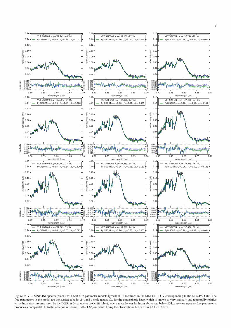
The hazes on Titan are known to not be uniform, so we fitthe SINFONI spectra with two variable haze models. We usea Levenberg-Marquardt (LM) optimization is to determine thesurface albedo, AS , and either one or two haze scale factors,fH , for each of the SINFONI spectra, which we refer to as “2-parameter” and “3-parameter” models, respectively. The freeparameters are well-constrained with reasonable initial esti-mates, justifying the LM optimization., SINFONI spectra alongthe region corresponding to the NIRSPAO slit are considered,and 12 of these spectra are plotted as examples in Figure 3, il-lustrating that these parameters are sufficient for interpreting theobservations. With χ2 ∼ 0.7 and 0.6 for the 2- and 3-parametermodels, respectively, the variable haze models are significantly

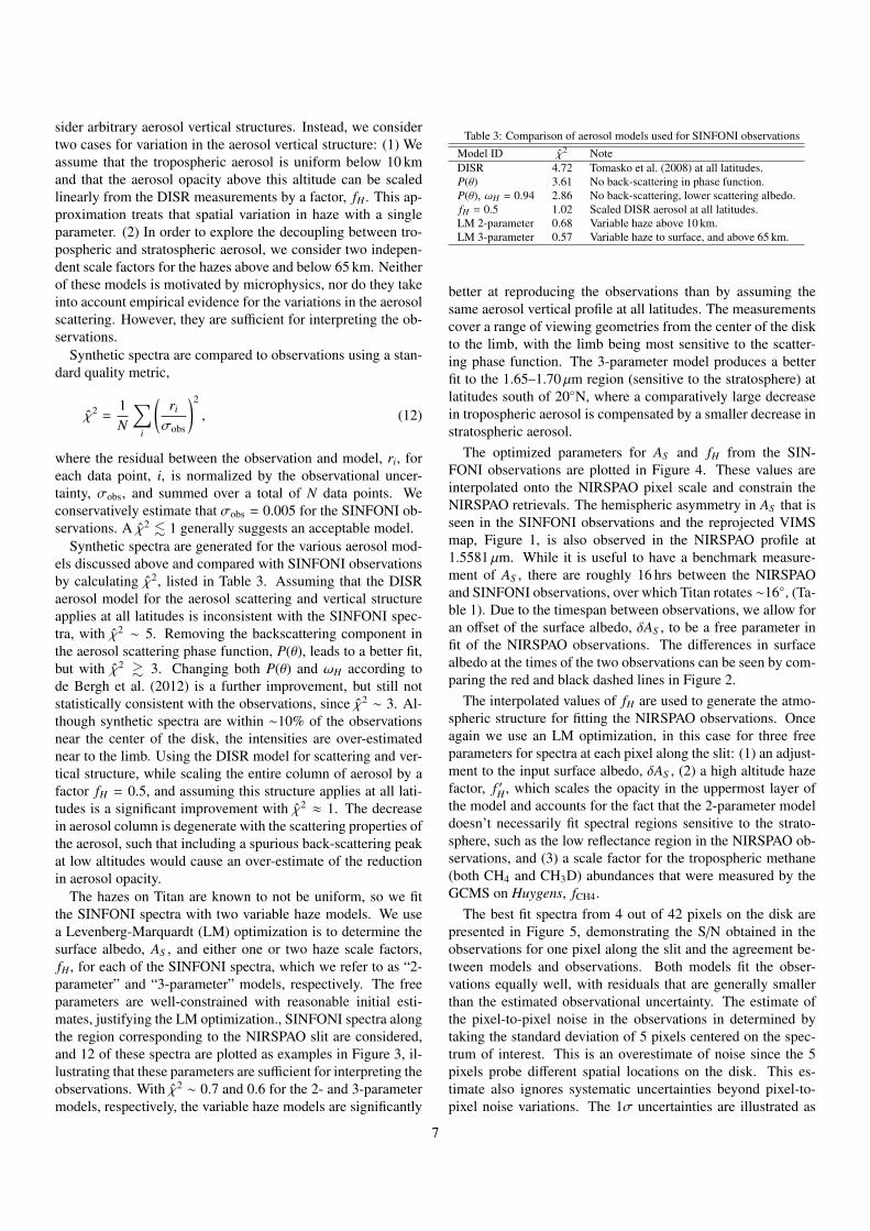
Table 3: Comparison of aerosol models used for SINFONI observations

Model ID χ2 NoteDISR 4.72 Tomasko et al. (2008) at all latitudes.P(θ) 3.61 No back-scattering in phase function.P(θ), ωH = 0.94 2.86 No back-scattering, lower scattering albedo.fH = 0.5 1.02 Scaled DISR aerosol at all latitudes.LM 2-parameter 0.68 Variable haze above 10 km.LM 3-parameter 0.57 Variable haze to surface, and above 65 km.

better at reproducing the observations than by assuming thesame aerosol vertical profile at all latitudes. The measurementscover a range of viewing geometries from the center of the diskto the limb, with the limb being most sensitive to the scatter-ing phase function. The 3-parameter model produces a betterfit to the 1.65–1.70 µm region (sensitive to the stratosphere) atlatitudes south of 20N, where a comparatively large decreasein tropospheric aerosol is compensated by a smaller decrease instratospheric aerosol.

The optimized parameters for AS and fH from the SIN-FONI observations are plotted in Figure 4. These values areinterpolated onto the NIRSPAO pixel scale and constrain theNIRSPAO retrievals. The hemispheric asymmetry in AS that isseen in the SINFONI observations and the reprojected VIMSmap, Figure 1, is also observed in the NIRSPAO profile at1.5581 µm. While it is useful to have a benchmark measure-ment of AS , there are roughly 16 hrs between the NIRSPAOand SINFONI observations, over which Titan rotates ∼16, (Ta-ble 1). Due to the timespan between observations, we allow foran offset of the surface albedo, δAS , to be a free parameter infit of the NIRSPAO observations. The differences in surfacealbedo at the times of the two observations can be seen by com-paring the red and black dashed lines in Figure 2.

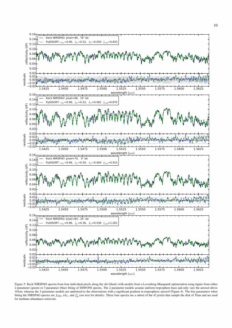
The interpolated values of fH are used to generate the atmo-spheric structure for fitting the NIRSPAO observations. Onceagain we use an LM optimization, in this case for three freeparameters for spectra at each pixel along the slit: (1) an adjust-ment to the input surface albedo, δAS , (2) a high altitude hazefactor, f ′H , which scales the opacity in the uppermost layer ofthe model and accounts for the fact that the 2-parameter modeldoesn’t necessarily fit spectral regions sensitive to the strato-sphere, such as the low reflectance region in the NIRSPAO ob-servations, and (3) a scale factor for the tropospheric methane(both CH4 and CH3D) abundances that were measured by theGCMS on Huygens, fCH4.

The best fit spectra from 4 out of 42 pixels on the disk arepresented in Figure 5, demonstrating the S/N obtained in theobservations for one pixel along the slit and the agreement be-tween models and observations. Both models fit the obser-vations equally well, with residuals that are generally smallerthan the estimated observational uncertainty. The estimate ofthe pixel-to-pixel noise in the observations in determined bytaking the standard deviation of 5 pixels centered on the spec-trum of interest. This is an overestimate of noise since the 5pixels probe different spatial locations on the disk. This es-timate also ignores systematic uncertainties beyond pixel-to-pixel noise variations. The 1σ uncertainties are illustrated as

7

8

0.02

0.04

0.06

0.08

0.10

0.12

0.14

0.16

reflect

ivit

y (

I/F)

VLT SINFONI: x,y=(37,14), -40 lat,

PyDISORT: ωH =0.96, fH =0.34, AS=0.027

1.50 1.55 1.60 1.65 1.70

wavelength (µm)

0.0100.0050.0000.0050.010

resi

duals

0.02

0.04

0.06

0.08

0.10

0.12

0.14

0.16

reflect

ivit

y (

I/F)


PyDISORT: ωH =0.96, fH =0.40, AS=0.050

1.50 1.55 1.60 1.65 1.70

wavelength (µm)

0.0100.0050.0000.0050.010

resi

duals

0.02

0.04

0.06

0.08

0.10

0.12

0.14

0.16

reflect

ivit

y (

I/F)


PyDISORT: ωH =0.96, fH =0.45, AS=0.046

1.50 1.55 1.60 1.65 1.70

wavelength (µm)

0.0100.0050.0000.0050.010

resi

duals

0.02

0.04

0.06

0.08

0.10

0.12

0.14

0.16

reflect

ivit

y (

I/F)

VLT SINFONI: x,y=(37,30), 0 lat,

PyDISORT: ωH =0.96, fH =0.47, AS=0.060

1.50 1.55 1.60 1.65 1.70

wavelength (µm)

0.0100.0050.0000.0050.010

resi

duals

0.02

0.04

0.06

0.08

0.10

0.12

0.14

0.16

reflect

ivit

y (

I/F)


PyDISORT: ωH =0.96, fH =0.51, AS=0.085

1.50 1.55 1.60 1.65 1.70

wavelength (µm)

0.0100.0050.0000.0050.010

resi

duals

0.02

0.04

0.06

0.08

0.10

0.12

0.14

0.16

reflect

ivit

y (

I/F)


PyDISORT: ωH =0.96, fH =0.52, AS=0.112

1.50 1.55 1.60 1.65 1.70

wavelength (µm)

0.0100.0050.0000.0050.010

resi

duals

0.02

0.04

0.06

0.08

0.10

0.12

0.14

0.16

reflect

ivit

y (

I/F)


PyDISORT: ωH =0.96, fH =0.54, AS=0.120

1.50 1.55 1.60 1.65 1.70

wavelength (µm)

0.0100.0050.0000.0050.010

resi

duals

0.02

0.04

0.06

0.08

0.10

0.12

0.14

0.16

reflect

ivit

y (

I/F)


PyDISORT: ωH =0.96, fH =0.55, AS=0.133

1.50 1.55 1.60 1.65 1.70

wavelength (µm)

0.0100.0050.0000.0050.010

resi

duals

0.02

0.04

0.06

0.08

0.10

0.12

0.14

0.16

reflect

ivit

y (

I/F)


PyDISORT: ωH =0.96, fH =0.59, AS=0.138

1.50 1.55 1.60 1.65 1.70

wavelength (µm)

0.0100.0050.0000.0050.010

resi

duals

0.02

0.04

0.06

0.08

0.10

0.12

0.14

0.16

reflect

ivit

y (

I/F)


PyDISORT: ωH =0.96, fH =0.63, AS=0.092

1.50 1.55 1.60 1.65 1.70

wavelength (µm)

0.0100.0050.0000.0050.010

resi

duals

0.02

0.04

0.06

0.08

0.10

0.12

0.14

0.16

reflect

ivit

y (

I/F)


PyDISORT: ωH =0.96, fH =0.60, AS=0.063

1.50 1.55 1.60 1.65 1.70

wavelength (µm)

0.0100.0050.0000.0050.010

resi

duals

0.02

0.04

0.06

0.08

0.10

0.12

0.14

0.16

reflect

ivit

y (

I/F)


PyDISORT: ωH =0.96, fH =0.49, AS=0.044

1.50 1.55 1.60 1.65 1.70

wavelength (µm)

0.0100.0050.0000.0050.010

resi

duals

Figure 3: VLT SINFONI spectra (black) with best fit 2-parameter models (green) at 12 locations in the SINFONI FOV corresponding to the NIRSPAO slit. Thefree parameters in the model are the surface albedo, AS , and a scale factor, fH , for the atmospheric haze, which is known to vary spatially and temporally relativeto the haze structure measured by the DISR. A 3-parameter model fit (blue), where scale factors for hazes above and below 65 km are two separate free parameters,produces a comparable fit to the observations from 1.50 – 1.62 µm, while fitting the observations better from 1.63 – 1.70 µm.

Figure 4: Parameters from LM optimization of model spectra fit to SINFONIobservations along the slit (a subset are shown in Figure 3), together with theNIRSPAO reflectivity at individual wavelengths (black) that are sensitive tothese parameters. The best fit surface albedos (top), where AS is always oneof the free parameters in the 2 and 3 parameters models (solid green and blue,respectively). And the haze scale factors, fH , (bottom panel) that are used foreither the entire vertical profile above 10 km (green dot-dash curve) or as twoseparate free parameters for the hazes above (blue dotted) and below 65 km(blue dashed). The 3-parameter model has a larger gradient in lower atmo-spheric haze than the 2-parameter model, and the stratospheric hazes decreasetoward both poles. The large haze gradient in the 3-parameter model is bal-anced by a small gradient in the surface albedo. The model parameters havebeen interpolated onto the NIRSPAO grid and are used as input parameters forfitting the NIRSPAO spectra.

the shaded gray regions in the residuals panel for each spec-trum in Figure 5. Parameters for each model are in the legend.

The LM optimization is performed for all spectra from 42Sto 80N using both haze models, assuming either spatially uni-form haze below 10 km or variable haze in this altitude region.Uncertainties are estimated using the roots of the diagonal ele-ments of the 3×3 covariance matrix of the LM optimization. Aplot of the latitudinal variation of fCH4 is presented in Figure 6for both model assumptions. In the case of uniform haze below10 km, there is a significant increase in tropospheric methanetoward the Southern Hemisphere and a slight depletion in theNorthern temperate regions, to ∼90% of the value measuredby the GCMS on Huygens. If the tropospheric aerosol is as-sumed to be variable, then the methane abundance is essentiallyuniform. The degeneracy between the tropospheric haze andmethane is due to the broadening and blending of methane linesat pressures above a bar. Increasing methane near the surfaceleads to smaller reflectivity at surface-probing wavelengths in

a manner similar to decreasing tropospheric aerosol. Indepen-dently constraining the spatial variation in tropospheric aerosolcan break the degeneracy between these two models.

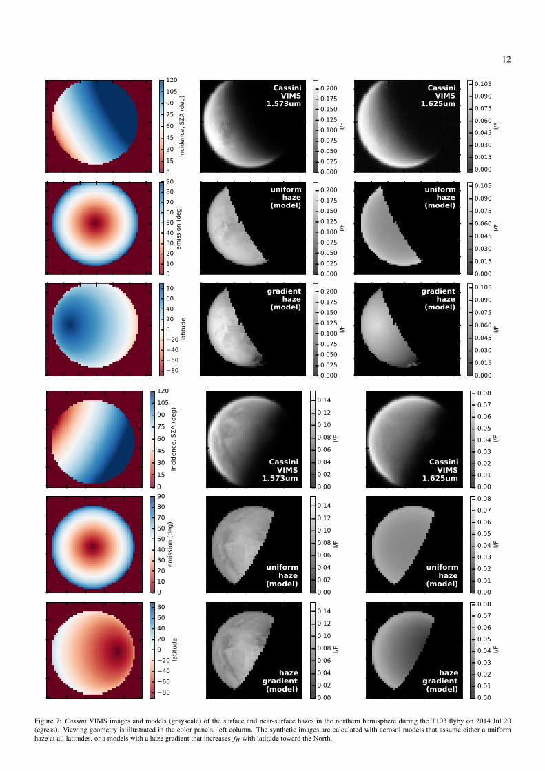
Three days after the ground-based observations there was aCassini flyby (T103) that passed over the Southern Hemisphereon ingress and over the Northern Hemisphere on egress, withVIMS recording global views of the polar regions of Titan. Fig-ures 7 show VIMS images from the 1.5 µm window in chan-nels that are sensitive to the surface (1.573 µm) and a neighbor-ing channel (1.625 µm) where the contribution from surface issmall. Differences in reflected intensity due to surface albedovariation can dominate those due to spatial variation in haze,so we calculate synthetic images for both channels, consider-ing either uniform haze, or a haze with a gradient of increasingopacity toward the North.

The synthetic 1.573 µm images in Figure 7 have decreasingsurface albedo contrast toward the limb and the terminator, dueto the increasing path length through the atmosphere associatedwith large incidence or emission angles. The greatest albedocontrast is near the dark, polar lakes in the Northern Hemi-sphere and near mid-latitudes in the Southern Hemisphere. As-suming a haze gradient leads to a brighter region near the pole,and slightly greater surface albedo contrast near the South Pole.In general, there are only minor differences in the synthetic im-ages of the surface when comparing the two haze models.

The synthetic 1.625 µm images, however, illustrate an in-creased sensitivity to the aerosol model. A uniform haze leadsto limb brightening that is consistent with observations both inthe North and the South polar regions, whereas the gradient inthe haze leads to brighter Northern, and a darker Southern, po-lar regions than are observed by VIMS. A uniform distributionof aerosol near the surface means that the NIRSPAO spectra andare more consistent with a meridional variation in methane, andnot a variation in aerosol.

5. Discussion

We have used complementary ground-based observationsfrom NIRSPAO at Keck and SINFONI at the VLT to measurethe tropospheric methane distribution on Titan. The spatially-resolved SINFONI observations at moderate resolution, acrossthe entire H-band, are used for the flux calibration and con-straining the aerosol haze distribution, while the high resolu-tion NIRSPAO observations are sensitive to the troposphericmethane. We used HITRAN 2012 line lists to generate kdistributions for CH4 and CH3D at the resolutions and platescales that correspond to each of the observations. Levenberg-Marquardt optimization was used to fit the observations, andretrieve the tropospheric methane abundance, assuming eithervariable or uniform tropospheric haze. Cassini VIMS imagessuggest that the haze is uniform toward both poles and that thereis meridional variation in methane.

The distribution of methane in Figure 6 reveals two interest-ing features. First, it is nearly uniform in the northern hemi-sphere from 15 N to the pole, and marginally lower (∼10%)than the Huygens GCMS measurement. Second, concentra-tions rise monotonically to the south of 15 N and reach a peak

9

10

0.02

0.04

0.06

0.08

0.10

0.12

0.14

0.16

reflect

ivit

y (

I/F)

Keck NIRSPAO: pixel=46, 78 lat

PyDISORT: ωH =0.96, fH =0.52, AS=0.050 fCH4=0.833

1.5425 1.5450 1.5475 1.5500 1.5525 1.5550 1.5575 1.5600 1.5625wavelength (µm)

0.020.010.000.010.02

resi

duals

0.02

0.04

0.06

0.08

0.10

0.12

0.14

0.16

reflect

ivit

y (

I/F)



1.5425 1.5450 1.5475 1.5500 1.5525 1.5550 1.5575 1.5600 1.5625wavelength (µm)

0.020.010.000.010.02

resi

duals

0.02

0.04

0.06

0.08

0.10

0.12

0.14

0.16

reflect

ivit

y (

I/F)



1.5425 1.5450 1.5475 1.5500 1.5525 1.5550 1.5575 1.5600 1.5625wavelength (µm)

0.020.010.000.010.02

resi

duals

0.02

0.04

0.06

0.08

0.10

0.12

0.14

0.16

reflect

ivit

y (

I/F)

Keck NIRSPAO: pixel=84, -35 lat


1.5425 1.5450 1.5475 1.5500 1.5525 1.5550 1.5575 1.5600 1.5625wavelength (µm)

0.020.010.000.010.02

resi

duals

Figure 5: Keck NIRSPAO spectra from four individual pixels along the slit (black) with models from a Levenberg-Marquardt optimization using inputs from either2-parameter (green) or 3-parameter (blue) fitting of SINFONI spectra. The 2-parameter models assume uniform troposphere haze and only vary the aerosol above10 km, whereas the 3-parameter models are optimized to the observations with a significant gradient in tropospheric aerosol (Figure 4). The free parameters whenfitting the NIRSPAO spectra are fCH4, δAS , and f ′H (see text for details). These four spectra are a subset of the 42 pixels that sample the disk of Titan and are usedfor methane abundance retrievals.

40 20 0 20 40 60 80

latitude

0.6

0.8

1.0

1.2

1.4

1.6

troposp

heri

c m

eth

ane s

cale

fact

or

uniform haze, z<10km

variable haze, z<10km

Figure 6: Meridional variation in the tropospheric methane abundance relativeto the mole fraction measured by the GCMS on the Huygens probe retrievedfrom fits to NIRSPAO spectra. Examples spectra and best-fit models are illus-trated in Figure 5.

value of 1.2-1.6 times the Huygens GCMS measurement at40 S. This suggests that there are at least two, distinct sourceregions of methane vapor, and that the atmosphere is mixingthe air masses from these source regions in latitudes south of15 N. If we assume the source regions produce saturated airmasses at the local temperature, we can estimate the differencein their temperatures. For a given temperature difference, ∆T ,the Clausius-Clapeyron relation predicts a fractional change insaturation vapor pressure, ∆es/es ≈ Lv∆T/(RvT 2), were Lv isthe latent heat of vaporization and Rv is the methane gas con-stant. Assuming the northern hemisphere source region has atemperature of ∼91 K, a 40% change in the saturation vaporpressure requires the source regions have a temperature differ-ence of ∼3 K, which is approximately the largest observed sur-face brightness temperature difference (Jennings et al., 2011).

Evaporation from Ontario Lacus (Turtle et al., 2011b; Hayeset al., 2011b) as the sole explanation for methane enhancement(during southern summer) was rejected by Tokano (2014) basedon the small spatial coverage of Ontario Lacus (0.04% of theSouthern hemisphere) and the assumption of ∼4 m change inlake depth. This suggests that lake evaporation at the poles overthe timescale of the Cassini mission is an unlikely explanationfor the increase in methane from the equator toward southernmid-latitudes at the onset of southern winter. However, evap-oration from moist ground or a number of small, methane-dominated lakes is still possible. Indeed, evaporation rates frommoist surfaces can exceed the rates from standing liquids dueto the larger surface area available and the possibility for in-creased turbulence above a rough surface. Our results suggestthat evaporation from the surface, in a region poleward of a par-ticular latitude, is increasing the relative humidity of the atmo-sphere. The observed gradient in methane abundance (towardthe winter pole) may then be an indication of a relatively moistair parcel from the pole equilibrating to the drier conditions atthe equator during meridional transport.

In November 2000, Anderson et al. (2008) used spectral im-ages from 0.6 – 1.0 µm, obtained with the Hubble Space Tele-scope (HST), to measure a latitudinal gradient from the southpole toward the northern (winter) mid-latitudes. They reportthat the tropospheric methane column roughly doubled from∼70S to ∼10N, and were presumably sensitive to to the nearsurface humidity. Since the HST observations were nearly ahalf Titan-year earlier, the seasons should be analogous to ourground-based observations, but mirrored North to South. Onedifference between the measurements is that Anderson et al.(2008) report a significant drop in the methane column in theirnorthern-most datapoint at ∼30N, whereas our measurementsincrease through ∼40S. Another consideration is that Ander-son et al. (2008) report a much weaker, or absent, latitudinalvariation in methane 7 days earlier at a different central merid-ian longitude (CML), which they speculate is an indication ofeither a surface or sub-surface source of methane that is spa-tially variable.

An increase in methane toward the winter polar is at oddswith the predictions of circulation models that have been usedto interpret Cassini radio occultation data. The measurementsobtained over the period from southern summer to southernequinox (2006-2009) indicate that tropospheric methane shouldincrease from the equator toward the Summer pole (Tokano,2014). The latitudinal gradient in sea-level pressures that areretrieved by Tokano (2014), assuming that methane increasestoward the Summer pole, are consistent with the location of theseasonal convergence zone and the observed regions of precip-itation as tracked by cloud formation (Mitchell, 2012). Furtherwork is required to determine conclusively if these observationstest particular assumptions of circulation models, e.g., the dis-tribution of methane at the surface, or if some other mecha-nism needs to be invoked to interpret the measurements. Forexample, episodic releases of methane, from some form of cry-ovolcanism, have been suggested as mechanism for supplyingthe moisture to southern mid-latitude clouds (Roe et al., 2005).However, the rate of cloud occurrence in the South has droppedwith the changing seasons and the locations of clouds are gen-erally thought to be controlled by circulation, rather than topog-raphy (Roe, 2012; Mitchell, 2012). Nonetheless, the propertiesof the surface regolith remain a mystery and the potential forthe episodic release of methane near polar latitudes is uncon-strained.

Repeated ground-based observations in different epochs, andat different CML can test for contemporary variability is near-surface sources of methane. If mixing of saturated polar air dur-ing transport controls the gradient in tropospheric methane, wecan predict that the gradient in methane should change season-ally with the changing circulation. Changes in the gradient onmore rapid time-scales, or at different CML can confirm eitherepisodic releases of methane or spatial variation in the sourceregion. Simultaneous observations with IFU and slit spectrom-eters, and quantitative constraints on the surface albedo fromVIMS maps could further constrain our models. Degenera-cies in the parameterized properties of the haze could also befurther constrained by aerosol microphysical models that pre-dict how the vertical structure of aerosol opacity and scattering

11

12

Cassini VIMS

1.573um

Cassini VIMS

1.625um

uniform haze

(model)

uniform haze

(model)

gradient haze

(model)

gradient haze

(model)

0.000

0.025

0.050

0.075

0.100

0.125

0.150

0.175

0.200

I/F

0.000

0.015

0.030

0.045

0.060

0.075

0.090

0.105

I/F

0.000

0.025

0.050

0.075

0.100

0.125

0.150

0.175

0.200

I/F

0.000

0.015

0.030

0.045

0.060

0.075

0.090

0.105

I/F

0.000

0.025

0.050

0.075

0.100

0.125

0.150

0.175

0.200

I/F

0.000

0.015

0.030

0.045

0.060

0.075

0.090

0.105

I/F

0

15

30

45

60

75

90

105

120

inci

dence

, SZ

A (

deg)

0

10

20

30

40

50

60

70

80

90em

issi

on (

deg)

80

60

40

20

0

20

40

60

80

lati

tude

Cassini VIMS

1.573um

Cassini VIMS

1.625um

uniform haze

(model)

uniform haze

(model)

haze gradient (model)

haze gradient (model)

0.00

0.02

0.04

0.06

0.08

0.10

0.12

0.14

I/F

0.00

0.01

0.02

0.03

0.04

0.05

0.06

0.07

0.08

I/F

0.00

0.02

0.04

0.06

0.08

0.10

0.12

0.14

I/F

0.00

0.01

0.02

0.03

0.04

0.05

0.06

0.07

0.08I/F

0.00

0.02

0.04

0.06

0.08

0.10

0.12

0.14

I/F

0.00

0.01

0.02

0.03

0.04

0.05

0.06

0.07

0.08

I/F

0

15

30

45

60

75

90

105

120

inci

dence

, SZ

A (

deg)

0

10

20

30

40

50

60

70

80

90

em

issi

on (

deg)

80

60

40

20

0

20

40

60

80

lati

tude

Figure 7: Cassini VIMS images and models (grayscale) of the surface and near-surface hazes in the northern hemisphere during the T103 flyby on 2014 Jul 20(egress). Viewing geometry is illustrated in the color panels, left column. The synthetic images are calculated with aerosol models that assume either a uniformhaze at all latitudes, or a models with a haze gradient that increases fH with latitude toward the North.

phase functions change with time. Continuing work on methaneline assignments, line shapes, and possible variations in upperstratospheric methane (e.g., Lellouch et al., 2014) can be usedto make quantitative improvements to both the relative and ab-solute uncertainties in the retrieval.

We have presented measurements of the meridional variationin tropospheric methane on Titan. These results suggest thatlocalized regions of evaporation occur at Southern polar lati-tudes in the winter, likely from a moist regolith. The simulta-neous analysis of Keck NIRSPAO, VLT SINFONI, and CassiniVIMS observations illustrate the challenges in performing anaccurate retrieval. We have mentioned a few improvements forconstraining assumptions in our radiative transfer models andhave suggested additional observations of this type at futureepochs. Accurately measuring the spatial variation in the tro-pospheric methane will constrain sources of methane at the sur-face and inform our understanding of the hydrological cycle onTitan.

Acknowledgements

This work was supported by NASA PAAST grantsNNX14AG82G and NNX12AM81G. MA was supported inpart by NSF AST-1008788. PMR was supported by Fondecytgrant #1120299. We wish to acknowledge Jonathan I. Lunineand Elizabeth P. Turtle, who are members of the VLT SINFONIcloud observing campaign that provided the SINFONI observa-tions presented here. Some of the data presented were obtainedat the W. M. Keck Observatory, which is operated as a scien-tific partnership among the California Institute of Technology,the University of California and the National Aeronautics andSpace Administration. The Observatory was made possible bythe generous financial support of the W. M. Keck Foundation.The authors wish to recognize the significant cultural role thatthe summit of Mauna Kea has always had within the indigenousHawaiian community. We are fortunate to have the opportunityto conduct observations from this mountain.

References

Adamkovics, M., Barnes, J. W., Hartung, M., de Pater, I., Aug. 2010. Ob-servations of a stationary mid-latitude cloud system on Titan. Icarus 208,868–877.

Adamkovics, M., de Pater, I., Hartung, M., Eisenhauer, F., Genzel, R., Griffith,C. A., Jun. 2006. Titan’s bright spots: Multiband spectroscopic measurementof surface diversity and hazes. Journal of Geophysical Research (Planets)111 (E7), E07S06.

Aharonson, O., Hayes, A. G., Lunine, J. I., Lorenz, R. D., Allison, M. D.,Elachi, C., Dec. 2009. An asymmetric distribution of lakes on Titan as apossible consequence of orbital forcing. Nature Geoscience 2, 851–854.

Anderson, C. M., Samuelson, R. E., Achterberg, R. K., Barnes, J. W., Flasar,F. M., Nov. 2014. Subsidence-induced methane clouds in Titan’s winter po-lar stratosphere and upper troposphere. Icarus 243, 129–138.

Anderson, C. M., Young, E. F., Chanover, N. J., McKay, C. P., Apr. 2008. HSTspectral imaging of Titan’s haze and methane profile between 0.6 and 1 µmduring the 2000 opposition. Icarus 194, 721–745.

Atreya, S. K., Adams, E. Y., Niemann, H. B., Demick-Montelara, J. E., Owen,T. C., Fulchignoni, M., Ferri, F., Wilson, E. H., Oct. 2006. Titan’s methanecycle. Planet. Space Sci. 54, 1177–1187.

Barnes, J. W., Bow, J., Schwartz, J., Brown, R. H., Soderblom, J. M., Hayes,A. G., Vixie, G., Le Mouelic, S., Rodriguez, S., Sotin, C., Jaumann, R.,Stephan, K., Soderblom, L. A., Clark, R. N., Buratti, B. J., Baines, K. H.,Nicholson, P. D., Nov. 2011. Organic sedimentary deposits in Titan’s drylakebeds: Probable evaporite. Icarus 216, 136–140.

Barth, E. L., Rafkin, S. C. R., Feb. 2007. TRAMS: A new dynamic cloud modelfor Titan’s methane clouds. Geophys. Res. Lett. 34 (3), L03203.

Brown, M. E., Roberts, J. E., Schaller, E. L., Feb. 2010. Clouds on Titan duringthe Cassini prime mission: A complete analysis of the VIMS data. Icarus205, 571–580.

Brown, M. E., Smith, A. L., Chen, C., Adamkovics, M., Nov. 2009. Discoveryof Fog at the South Pole of Titan. Astrophys. J. Lett. 706 (1), L110–L113.

Brown, R. H., Baines, K. H., Bellucci, G., Bibring, J.-P., Buratti, B. J., Capac-cioni, F., Cerroni, P., Clark, R. N., Coradini, A., Cruikshank, D. P., Drossart,P., Formisano, V., Jaumann, R., Langevin, Y., Matson, D. L., McCord,T. B., Mennella, V., Miller, E., Nelson, R. M., Nicholson, P. D., Sicardy,B., Sotin, C., Dec. 2004. The Cassini Visual And Infrared Mapping Spec-trometer (Vims) Investigation. Space Science Reviews 115, 111–168.

Brown, R. H., Soderblom, L. A., Soderblom, J. M., Clark, R. N., Jaumann, R.,Barnes, J. W., Sotin, C., Buratti, B., Baines, K. H., Nicholson, P. D., Jul.2008. The identification of liquid ethane in Titan’s Ontario Lacus. Nature454, 607–610.

Campargue, A., Wang, L., Mondelain, D., Kassi, S., Bezard, B., Lellouch, E.,Coustenis, A., Bergh, C. d., Hirtzig, M., Drossart, P., May 2012. An empir-ical line list for methane in the 1.26-1.71 µm region for planetary investiga-tions (T = 80-300 K). Application to Titan. Icarus 219, 110–128.

Cohen, M., Wheaton, W. A., Megeath, S. T., Aug. 2003. Spectral IrradianceCalibration in the Infrared. XIV. The Absolute Calibration of 2MASS. AJ126, 1090–1096.

Cornet, T., Bourgeois, O., Le Mouelic, S., Rodriguez, S., Sotin, C., Barnes,J. W., Brown, R. H., Baines, K. H., Buratti, B. J., Clark, R. N., Nicholson,P. D., Jul. 2012. Edge detection applied to Cassini images reveals no measur-able displacement of Ontario Lacus’ margin between 2005 and 2010. Journalof Geophysical Research (Planets) 117, 7005.

Cutri, R. M., Skrutskie, M. F., van Dyk, S., Beichman, C. A., Carpenter, J. M.,Chester, T., Cambresy, L., Evans, T., Fowler, J., Gizis, J., Howard, E.,Huchra, J., Jarrett, T., Kopan, E. L., Kirkpatrick, J. D., Light, R. M., Marsh,K. A., McCallon, H., Schneider, S., Stiening, R., Sykes, M., Weinberg, M.,Wheaton, W. A., Wheelock, S., Zacarias, N., Mar. 2003. 2MASS All-SkyCatalog of Point Sources (Cutri+ 2003). VizieR Online Data Catalog 2246,0.

de Bergh, C., Courtin, R., Bezard, B., Coustenis, A., Lellouch, E., Hirtzig, M.,Rannou, P., Drossart, P., Campargue, A., Kassi, S., Wang, L., Boudon, V.,Nikitin, A., Tyuterev, V., Feb. 2012. Applications of a new set of methaneline parameters to the modeling of Titan’s spectrum in the 1.58 µm window.Planet. Space Sci. 61, 85–98.

Eisenhauer, F., Abuter, R., Bickert, K., Biancat-Marchet, F., Bonnet, H., Bryn-nel, J., Conzelmann, R. D., Delabre, B., Donaldson, R., Farinato, J., Fedrigo,E., Genzel, R., Hubin, N. N., Iserlohe, C., Kasper, M. E., Kissler-Patig, M.,Monnet, G. J., Roehrle, C., Schreiber, J., Stroebele, S., Tecza, M., Thatte,N. A., Weisz, H., Mar. 2003. SINFONI - Integral field spectroscopy at 50milli-arcsecond resolution with the ESO VLT. In: Instrument Design andPerformance for Optical/Infrared Ground-based Telescopes. Edited by Iye,Masanori; Moorwood, Alan F. M. Proceedings of the SPIE, Volume 4841,pp. 1548-1561 (2003). pp. 1548–1561.

Friedson, A. J., West, R. A., Wilson, E. H., Oyafuso, F., Orton, G. S., Dec. 2009.A global climate model of Titan’s atmosphere and surface. Planet. Space Sci.57, 1931–1949.

Fulchignoni, M., Ferri, F., Angrilli, F., Ball, A. J., Bar-Nun, A., Barucci, M. A.,Bettanini, C., Bianchini, G., Borucki, W., Colombatti, G., Coradini, M.,Coustenis, A., Debei, S., Falkner, P., Fanti, G., Flamini, E., Gaborit, V.,Grard, R., Hamelin, M., Harri, A. M., Hathi, B., Jernej, I., Leese, M. R.,Lehto, A., Lion Stoppato, P. F., Lopez-Moreno, J. J., Makinen, T., McDon-nell, J. A. M., McKay, C. P., Molina-Cuberos, G., Neubauer, F. M., Pir-ronello, V., Rodrigo, R., Saggin, B., Schwingenschuh, K., Seiff, A., Simoes,F., Svedhem, H., Tokano, T., Towner, M. C., Trautner, R., Withers, P., Zar-necki, J. C., Dec. 2005. In situ measurements of the physical characteristicsof Titan’s environment. Nature 438, 785–791.

Griffith, C. A., Doose, L., Tomasko, M. G., Penteado, P. F., See, C., Apr. 2012a.Radiative transfer analyses of Titan’s tropical atmosphere. Icarus 218, 975–988.

13

Griffith, C. A., Lora, J. M., Turner, J., Penteado, P. F., Brown, R. H., Tomasko,M. G., Doose, L., See, C., Jun. 2012b. Possible tropical lakes on Titan fromobservations of dark terrain. Nature 486, 237–239.

Griffith, C. A., Penteado, P., Baines, K., Drossart, P., Barnes, J., Bellucci, G.,Bibring, J., Brown, R., Buratti, B., Capaccioni, F., Cerroni, P., Clark, R.,Combes, M., Coradini, A., Cruikshank, D., Formisano, V., Jaumann, R.,Langevin, Y., Matson, D., McCord, T., Mennella, V., Nelson, R., Nicholson,P., Sicardy, B., Sotin, C., Soderblom, L. A., Kursinski, R., Oct. 2005. TheEvolution of Titan’s Mid-Latitude Clouds. Science 310, 474–477.

Hayes, A., Aharonson, O., Callahan, P., Elachi, C., Gim, Y., Kirk, R., Lewis, K.,Lopes, R., Lorenz, R., Lunine, J., Mitchell, K., Mitri, G., Stofan, E., Wall,S., May 2008. Hydrocarbon lakes on Titan: Distribution and interaction witha porous regolith. Geophysical Research Letters 35, L9204.

Hayes, A. G., Aharonson, O., Lunine, J. I., Kirk, R. L., Zebker, H. A., Wye,L. C., Lorenz, R. D., Turtle, E. P., Paillou, P., Mitri, G., Wall, S. D., Stofan,E. R., Mitchell, K. L., Elachi, C., Cassini Radar Team, Jan. 2011a. Transientsurface liquid in Titan’s polar regions from Cassini. Icarus 211, 655–671.

Hayes, A. G., Aharonson, O., Lunine, J. I., Kirk, R. L., Zebker, H. A., Wye,L. C., Lorenz, R. D., Turtle, E. P., Paillou, P., Mitri, G., Wall, S. D., Stofan,E. R., Mitchell, K. L., Elachi, C., the Cassini RADAR Team, Jan. 2011b.Transient surface liquid in Titan’s polar regions from Cassini. Icarus 211,655–671.

Hirtzig, M., Bezard, B., Lellouch, E., Coustenis, A., de Bergh, C., Drossart,P., Campargue, A., Boudon, V., Tyuterev, V., Rannou, P., Cours, T., Kassi,S., Nikitin, A., Mondelain, D., Rodriguez, S., Le Mouelic, S., Sep. 2013.Corrigendum to ”Titan’s surface and atmosphere from Cassini/VIMS datawith updated methane opacity” [Icarus 226 (2013) 470-486]. Icarus 226,1182–1182.

Hueso, R., Sanchez-Lavega, A., Jul. 2006. Methane storms on Saturn’s moonTitan. Nature 442, 428–431.

Iess, L., Rappaport, N. J., Jacobson, R. A., Racioppa, P., Stevenson, D. J., Tor-tora, P., Armstrong, J. W., Asmar, S. W., Mar. 2010. Gravity Field, Shape,and Moment of Inertia of Titan. Science 327, 1367–.

Irwin, P. G. J., Lellouch, E., de Bergh, C., Courtin, R., Bezard, B., Fletcher,L. N., Orton, G. S., Teanby, N. A., Calcutt, S. B., Tice, D., Hurley, J., Davis,G. R., Jan. 2014. Line-by-line analysis of Neptune’s near-IR spectrum ob-served with Gemini/NIFS and VLT/CRIRES. Icarus 227, 37–48.

Jennings, D. E., Cottini, V., Nixon, C. A., Flasar, F. M., Kunde, V. G., Samuel-son, R. E., Romani, P. N., Hesman, B. E., Carlson, R. C., Gorius, N. J. P.,Coustenis, A., Tokano, T., 2011. Seasonal changes in titan’s surface temper-atures. The Astrophysical Journal Letters 737 (1), L15.URL http://stacks.iop.org/2041-8205/737/i=1/a=L15

Lacis, A. A., Oinas, V., May 1991. A description of the correlated-k distribu-tion method for modelling nongray gaseous absorption, thermal emission,and multiple scattering in vertically inhomogeneous atmospheres. J. Geo-phys. Res. 96, 9027–9064.

Le Gall, A., Janssen, M. A., Wye, L. C., Hayes, A. G., Radebaugh, J., Savage,C., Zebker, H., Lorenz, R. D., Lunine, J. I., Kirk, R. L., Lopes, R. M. C.,Wall, S., Callahan, P., Stofan, E. R., Farr, T., Jun. 2011. Cassini SAR, ra-diometry, scatterometry and altimetry observations of Titan’s dune fields.Icarus 213, 608–624.

Lellouch, E., Bezard, B., Flasar, F. M., Vinatier, S., Achterberg, R., Nixon,C. A., Bjoraker, G. L., Gorius, N., Mar. 2014. The distribution of methane inTitan’s stratosphere from Cassini/CIRS observations. Icarus 231, 323–337.

Lora, J. M., Lunine, J. I., Russell, J. L., Hayes, A. G., Nov. 2014. Simulationsof Titan’s paleoclimate. Icarus 243, 264–273.

Lorenz, R. D., Aug. 2014. The flushing of Ligeia: Composition variationsacross Titan’s seas in a simple hydrological model. Geophys. Res. Lett. 41,5764–5770.

Lorenz, R. D., Kirk, R. L., Hayes, A. G., Anderson, Y. Z., Lunine, J. I., Tokano,T., Turtle, E. P., Malaska, M. J., Soderblom, J. M., Lucas, A., Karatekin, O.,Wall, S. D., Jul. 2014. A radar map of Titan Seas: Tidal dissipation andocean mixing through the throat of Kraken. Icarus 237, 9–15.

Lorenz, R. D., Mitchell, K. L., Kirk, R. L., Hayes, A. G., Aharonson, O., Ze-bker, H. A., Paillou, P., Radebaugh, J., Lunine, J. I., Janssen, M. A., Wall,S. D., Lopes, R. M., Stiles, B., Ostro, S., Mitri, G., Stofan, E. R., Jan. 2008.Titan’s inventory of organic surface materials. Geophys. Res. Lett. 35, 2206.

Lorenz, R. D., Smith, P. H., Lemmon, M. T., May 2004. Seasonal change in Ti-tan’s haze 1992-2002 from Hubble Space Telescope observations. Geophys.Res. Lett. 31, 10702–+.

Lorenz, R. D., Stiles, B. W., Aharonson, O., Lucas, A., Hayes, A. G., Kirk,

R. L., Zebker, H. A., Turtle, E. P., Neish, C. D., Stofan, E. R., Barnes, J. W.,Jul. 2013. A global topographic map of Titan. Icarus 225, 367–377.

Lorenz, R. D., Wall, S., Radebaugh, J., Boubin, G., Reffet, E., Janssen, M.,Stofan, E., Lopes, R., Kirk, R., Elachi, C., Lunine, J., Mitchell, K., Pa-ganelli, F., Soderblom, L., Wood, C., Wye, L., Zebker, H., Anderson, Y.,Ostro, S., Allison, M., Boehmer, R., Callahan, P., Encrenaz, P., Ori, G. G.,Francescetti, G., Gim, Y., Hamilton, G., Hensley, S., Johnson, W., Kelle-her, K., Muhleman, D., Picardi, G., Posa, F., Roth, L., Seu, R., Shaffer, S.,Stiles, B., Vetrella, S., Flamini, E., West, R., May 2006. The Sand Seas ofTitan: Cassini RADAR Observations of Longitudinal Dunes. Science 312,724–727.

MacKenzie, S. M., Barnes, J. W., Sotin, C., Soderblom, J. M., Mouelic, S. L.,Rodriguez, S., Baines, K. H., Buratti, B. J., Clark, R. N., Nicholson, P. D.,McCord, T. B., 2014. Evidence of titan’s climate history from evaporite dis-tribution. Icarus 243, 191 – 207.

Mastrogiuseppe, M., Poggiali, V., Hayes, A., Lorenz, R., Lunine, J., Picardi,G., Seu, R., Flamini, E., Mitri, G., Notarnicola, C., Paillou, P., Zebker, H.,2014. The bathymetry of a titan sea. Geophysical Research Letters 41 (5),1432–1437.URL http://dx.doi.org/10.1002/2013GL058618

McLean, I. S., Becklin, E. E., Bendiksen, O., Brims, G., Canfield, J., Figer,D. F., Graham, J. R., Hare, J., Lacayanga, F., Larkin, J. E., Larson, S. B.,Levenson, N., Magnone, N., Teplitz, H., Wong, W., Aug. 1998. Designand development of NIRSPEC: a near-infrared echelle spectrograph for theKeck II telescope. In: Fowler, A. M. (Ed.), Infrared Astronomical Instru-mentation. Vol. 3354 of Society of Photo-Optical Instrumentation Engineers(SPIE) Conference Series. pp. 566–578.

Mitchell, J. L., Sep. 2012. Titan’s Transport-driven Methane Cycle. ApJ 756,L26.

Mitchell, J. L., Adamkovics, M., Caballero, R., Turtle, E. P., Sep. 2011. Locallyenhanced precipitation organized by planetary-scale waves on Titan. NatureGeoscience 4, 589–592.

Mitchell, J. L., Pierrehumbert, R. T., Frierson, D. M. W., Caballero, R., Sep.2009. The impact of methane thermodynamics on seasonal convection andcirculation in a model Titan atmosphere. Icarus 203, 250–264.

Mitri, G., Showman, A. P., Lunine, J. I., Lorenz, R. D., Feb. 2007. Hydrocarbonlakes on Titan. Icarus 186, 385–394.

Moore, J. M., Howard, A. D., Nov. 2010. Are the basins of Titan’s Hotei Regioand Tui Regio sites of former low latitude seas? Geophys. Res. Lett. 37,L22205.

Niemann, H. B., Atreya, S. K., Bauer, S. J., Carignan, G. R., Demick, J. E.,Frost, R. L., Gautier, D., Haberman, J. A., Harpold, D. N., Hunten, D. M., Is-rael, G., Lunine, J. I., Kasprzak, W. T., Owen, T. C., Paulkovich, M., Raulin,F., Raaen, E., Way, S. H., Dec. 2005. The abundances of constituents of Ti-tan’s atmosphere from the GCMS instrument on the Huygens probe. Nature438, 779–784.

Niemann, H. B., Atreya, S. K., Demick, J. E., Gautier, D., Haberman, J. A.,Harpold, D. N., Kasprzak, W. T., Lunine, J. I., Owen, T. C., Raulin, F., Dec.2010. Composition of Titan’s lower atmosphere and simple surface volatilesas measured by the Cassini-Huygens probe gas chromatograph mass spec-trometer experiment. Journal of Geophysical Research (Planets) 115 (E14),12006.

Penteado, P. F., Griffith, C. A., Mar. 2010. Ground-based measurements of themethane distribution on Titan. Icarus 206, 345–351.

Radebaugh, J., Lorenz, R. D., Lunine, J. I., Wall, S. D., Boubin, G., Reffet,E., Kirk, R. L., Lopes, R. M., Stofan, E. R., Soderblom, L., Allison, M.,Janssen, M., Paillou, P., Callahan, P., Spencer, C., The Cassini Radar Team,Apr. 2008. Dunes on Titan observed by Cassini Radar. Icarus 194, 690–703.

Rannou, P., Montmessin, F., Hourdin, F., Lebonnois, S., Jan. 2006. The Latitu-dinal Distribution of Clouds on Titan. Science 311, 201–205.

Rodriguez, S., Garcia, A., Lucas, A., Appere, T., Le Gall, A., Reffet, E., LeCorre, L., Le Mouelic, S., Cornet, T., Courrech du Pont, S., Narteau, C.,Bourgeois, O., Radebaugh, J., Arnold, K., Barnes, J. W., Stephan, K., Jau-mann, R., Sotin, C., Brown, R. H., Lorenz, R. D., Turtle, E. P., Feb. 2014.Global mapping and characterization of Titan’s dune fields with Cassini:Correlation between RADAR and VIMS observations. Icarus 230, 168–179.

Rodriguez, S., Le Mouelic, S., Rannou, P., Sotin, C., Brown, R. H., Barnes,J. W., Griffith, C. A., Burgalat, J., Baines, K. H., Buratti, B. J., Clark, R. N.,Nicholson, P. D., Nov. 2011. Titan’s cloud seasonal activity from winter tospring with Cassini/VIMS. Icarus 216, 89–110.

Rodriguez, S., Le Mouelic, S., Rannou, P., Tobie, G., Baines, K. H., Barnes,

14

J. W., Griffith, C. A., Hirtzig, M., Pitman, K. M., Sotin, C., Brown, R. H.,Buratti, B. J., Clark, R. N., Nicholson, P. D., Jun. 2009. Global circulationas the main source of cloud activity on Titan. Nature 459, 678–682.

Roe, H. G., May 2012. Titan’s Methane Weather. Annual Review of Earth andPlanetary Sciences 40, 355–382.

Roe, H. G., Brown, M. E., Schaller, E. L., Bouchez, A. H., Trujillo, C. A.,Oct. 2005. Geographic Control of Titan’s Mid-Latitude Clouds. Science 310,477–479.

Rothman, L. S., Gordon, I. E., Babikov, Y., Barbe, A., Chris Benner, D.,Bernath, P. F., Birk, M., Bizzocchi, L., Boudon, V., Brown, L. R., Cam-pargue, A., Chance, K., Cohen, E. A., Coudert, L. H., Devi, V. M., Drouin,B. J., Fayt, A., Flaud, J.-M., Gamache, R. R., Harrison, J. J., Hartmann,J.-M., Hill, C., Hodges, J. T., Jacquemart, D., Jolly, A., Lamouroux, J., LeRoy, R. J., Li, G., Long, D. A., Lyulin, O. M., Mackie, C. J., Massie, S. T.,Mikhailenko, S., Muller, H. S. P., Naumenko, O. V., Nikitin, A. V., Orphal,J., Perevalov, V., Perrin, A., Polovtseva, E. R., Richard, C., Smith, M. A. H.,Starikova, E., Sung, K., Tashkun, S., Tennyson, J., Toon, G. C., Tyuterev,V. G., Wagner, G., Nov. 2013. The HITRAN2012 molecular spectroscopicdatabase. J. Quant. Spec. Radiat. Transf. 130, 4–50.

Schneider, T., Graves, S. D. B., Schaller, E. L., Brown, M. E., Jan. 2012. Po-lar methane accumulation and rainstorms on Titan from simulations of themethane cycle. Nature 481, 58–61.

Sotin, C., Lawrence, K. J., Reinhardt, B., Barnes, J. W., Brown, R. H., Hayes,A. G., Le Mouelic, S., Rodriguez, S., Soderblom, J. M., Soderblom, L. A.,Baines, K. H., Buratti, B. J., Clark, R. N., Jaumann, R., Nicholson, P. D.,Stephan, K., Nov. 2012. Observations of Titan’s Northern lakes at 5 µm:Implications for the organic cycle and geology. Icarus 221, 768–786.

Sromovsky, L. A., Fry, P. M., Boudon, V., Campargue, A., Nikitin, A., Mar.2012. Comparison of line-by-line and band models of near-IR methane ab-sorption applied to outer planet atmospheres. Icarus 218, 1–23.

Stamnes, K., Tsay, S.-C., Jayaweera, K., Wiscombe, W., 1988. Numericallystable algorithm for discrete-ordinate-method radiative transfer in multiplescattering and emitting layered media. Applied Optics 27, 2502–2509.

Stofan, E. R., Elachi, C., Lunine, J. I., Lorenz, R. D., Stiles, B., Mitchell, K. L.,Ostro, S., Soderblom, L., Wood, C., Zebker, H., Wall, S., Janssen, M., Kirk,R., Lopes, R., Paganelli, F., Radebaugh, J., Wye, L., Anderson, Y., Allison,M., Boehmer, R., Callahan, P., Encrenaz, P., Flamini, E., Francescetti, G.,Gim, Y., Hamilton, G., Hensley, S., Johnson, W. T. K., Kelleher, K., Muh-leman, D., Paillou, P., Picardi, G., Posa, F., Roth, L., Seu, R., Shaffer, S.,Vetrella, S., West, R., Jan. 2007. The lakes of Titan. Nature 445, 61–64.

Tokano, T., Mar. 2009. Limnological Structure of Titan’s Hydrocarbon Lakesand Its Astrobiological Implication. Astrobiology 9, 147–164.

Tokano, T., Mar. 2014. Non-uniform global methane distribution in Titan’s tro-posphere evidenced by Cassini radio occultations. Icarus 231, 1–12.

Tomasko, M. G., Doose, L., Engel, S., Dafoe, L. E., West, R., Lemmon, M.,Karkoschka, E., See, C., Apr. 2008. A model of Titan’s aerosols based onmeasurements made inside the atmosphere. Planet. Space Sci. 56, 669–707.

Turtle, E. P., Perry, J. E., Hayes, A. G., Lorenz, R. D., Barnes, J. W., McEwen,A. S., West, R. A., Del Genio, A. D., Barbara, J. M., Lunine, J. I., Schaller,E. L., Ray, T. L., Lopes, R. M. C., Stofan, E. R., Mar. 2011a. Rapid and Ex-tensive Surface Changes Near Titan’s Equator: Evidence of April Showers.Science 331, 1414–.

Turtle, E. P., Perry, J. E., Hayes, A. G., McEwen, A. S., Apr. 2011b. Shorelineretreat at Titan’s Ontario Lacus and Arrakis Planitia from Cassini ImagingScience Subsystem observations. Icarus 212, 957–959.

Turtle, E. P., Perry, J. E., McEwen, A. S., Del Genio, A. D., Barbara, J., West,R. A., Dawson, D. D., Porco, C. C., Jan. 2009. Cassini imaging of Titan’shigh-latitude lakes, clouds, and south-polar surface changes. Geophys. Res.Lett. 36 (2), L02204.

Vixie, G., Barnes, J. W., Jackson, B., Rodriguez, S., Le Mouelic, S., Wilson, P.,2014. Two Temperate Lakes on Titan. J. Geophys. Res. , in revision.

15

Documents

Meridional variation in tropospheric methane on Titan