Embed Size (px)
Citation preview
Merge Strategies
for Merge-and-Shrink Heuristics
Master’s Thesis
Natural Science Faculty of the University of Basel
Department of Mathematics and Computer Science
Artificial Intelligence
http://ai.cs.unibas.ch/
Examiner: Prof. Dr. Malte Helmert
Supervisor: Silvan Sievers, Dr. Martin Wehrle
Daniel Federau
11-057-197
03.02.2017

Acknowledgments
At this point I would like to thank Silvan Sievers and Dr. Martin Wehrle for their help and
insight during the last six months. I would also like to thank Prof. Dr. Malte Helmert for
allowing me to write this master’s thesis in the area of Artificial Intelligence. Last but not
least, I would like to thank my parents and friends for their support.
Abstract
The merge-and-shrink heuristic is a state-of-the-art admissible heuristic that is often used
for optimal planning. Recent studies showed that the merge strategy is an important factor
for the performance of the merge-and-shrink algorithm. There are many different merge
strategies and improvements for merge strategies described in the literature. One out of these
merge strategies is MIASM by Fan et al. [4]. MIASM tries to merge transition systems that
produce unnecessary states in their product which can be pruned. Another merge strategy is
the symmetry-based merge-and-shrink framework by Sievers et al. [13]. This strategy tries to
merge transition systems that cause factored symmetries in their product. This strategy can
be combined with other merge strategies and it often improves the performance for many
merge strategy. However, the current combination of MIASM with factored symmetries
performs worse than MIASM. We implement a different combination of MIASM that uses
factored symmetries during the subset search of MIASM. Our experimental evaluation shows
that our new combination of MIASM with factored symmetries solves more tasks than the
existing MIASM and the previously implemented combination of MIASM with factored
symmetries. We also evaluate different combinations of existing merge strategies and find
combinations that perform better than their basic version that were not evaluated before.
Table of Contents
Acknowledgments i
Abstract ii
1 Introduction 1
2 Background 4
2.1 Classical Planning . . . . . . . . . . . . . . . . . . . . . . . . . . . . . . . . . 4
2.2 The Merge-and-Shrink Heuristic . . . . . . . . . . . . . . . . . . . . . . . . . 5
2.3 A Collection of Merge Strategies . . . . . . . . . . . . . . . . . . . . . . . . . 7
2.3.1 Linear Merge Strategies . . . . . . . . . . . . . . . . . . . . . . . . . . 7
2.3.2 DFP . . . . . . . . . . . . . . . . . . . . . . . . . . . . . . . . . . . . . 8
2.3.3 MIASM . . . . . . . . . . . . . . . . . . . . . . . . . . . . . . . . . . . 8
2.3.4 Dynamic MIASM . . . . . . . . . . . . . . . . . . . . . . . . . . . . . . 9
2.3.5 SCC-DFP . . . . . . . . . . . . . . . . . . . . . . . . . . . . . . . . . . 9
2.3.6 Tie-Breaking for Dynamic Merge Strategies . . . . . . . . . . . . . . . 10
2.4 Factored Symmetries for Merge Strategies . . . . . . . . . . . . . . . . . . . . 10
3 Experimental Evaluation of Merge Strategies 12
3.1 Experimental Setup and Evaluated Attributes . . . . . . . . . . . . . . . . . . 12
3.2 Overview . . . . . . . . . . . . . . . . . . . . . . . . . . . . . . . . . . . . . . 13
3.3 DFP with Symmetries and Tie-Breaking . . . . . . . . . . . . . . . . . . . . . 14
3.4 Dynamic MIASM with Symmetries . . . . . . . . . . . . . . . . . . . . . . . . 15
3.5 SCC with Dynamic MIASM . . . . . . . . . . . . . . . . . . . . . . . . . . . . 16
3.6 Conclusion . . . . . . . . . . . . . . . . . . . . . . . . . . . . . . . . . . . . . 17
4 MIASM with Factored Symmetries 18
4.1 Previous Implementation of SYMM-MIASM . . . . . . . . . . . . . . . . . . . 18
4.2 MIASM-Subset Search . . . . . . . . . . . . . . . . . . . . . . . . . . . . . . . 18
4.3 Subset-Initialisation with Symmetries . . . . . . . . . . . . . . . . . . . . . . 19
4.4 Hill Climbing Search for Factored Symmetries . . . . . . . . . . . . . . . . . . 20
5 Experimental Results 22
5.1 Overview . . . . . . . . . . . . . . . . . . . . . . . . . . . . . . . . . . . . . . 22
5.2 Domain-specific evaluation . . . . . . . . . . . . . . . . . . . . . . . . . . . . . 24
5.2.1 MIASM against HC-Combo . . . . . . . . . . . . . . . . . . . . . . . . 24
5.2.2 SYMM-MIASM against HC-Combo . . . . . . . . . . . . . . . . . . . 25
6 Conclusion 27

Table of Contents iv
Bibliography 28
1Introduction
Classical planning is a frequently researched topic in the field of Artificial Intelligence. The
goal of planning is to find a solution (i.e. a plan) for a given problem. A plan consists of a
sequence of actions that leads from an initial state to a goal state. One approach for finding
a plan is to use search algorithms. Search algorithms search for a plan in the state space of
a planning task. However, for big problems, the state space can become very large which
means it is no longer possible to find a plan within a reasonable amount of time or memory.
A way to improve the performance of search algorithms is to use heuristic functions. A
heuristic function estimates the remaining cost from the current state to a goal state. These
heuristic values lead the search algorithm towards a goal. A popular search algorithm that
uses heuristics is the A∗ algorithm [5]. A∗ that uses an admissible heuristic (i.e. a heuristic
that is always smaller or equal than the actual lowest cost to a goal) finds plans that are
optimal, i.e. the plan with the smallest cost out of all possible plans.
There are many different heuristics described in the literature. One group out of them
are the abstraction-based heuristics. An abstraction is a mapping of the state space of a
planning task that reduces the number of states by merging several states into one state.
The cost of an optimal plan from an abstract state s to an abstract goal state is then used
as a heuristic value for the corresponding state of s in the original state space.
One way to obtain heuristic values based on abstractions is by using the merge-and-
shrink algorithm. It was first introduced for model checking by Drager et al. [2, 3] and was
adapted for classical planning by Helmert et al. [7, 8]. The algorithm starts with a set of
atomic transition systems (one transition system for every variable of the planning task). It
then chooses two transition systems out of the set according to a merge strategy and replaces
them with the merged transition system (merge-step). Before merging, the algorithm checks
whether the size of the merged transition system surpasses a previously defined limit. If it
does, the algorithm will perform a shrink-step to reduce the number of states of one or both
of the transition systems to be merged according to a shrink-strategy. These steps will be
repeated until only one transition system is left. The cost of the optimal plan to a goal in
this last transition system will then be used as a heuristic value for the planning task.
There are different merge strategies proposed in the literature that we can use for the
merge-step. Experiments show that the choice of merge strategies influences the performance
Introduction 2
of the merge-and-shrink heuristic [12]. So it makes sense to further explore the effects of
merge strategies. Linear merge strategies are the first strategies that were used for planning.
A linear merge strategy always merges one atomic transition system with one non-atomic,
except in the beginning, when there are only atomic transition systems to choose from. The
first non-linear merge strategy for classical planning is DFP. It was first used for model check-
ing [2, 3] and was implemented by Sievers, Wehrle and Helmert [11] for classical planning.
DFP computes a weight for every pair of abstractions and chooses the pair with the lowest
weight as the next merge. Another non-linear merge strategy is MIASM by Fan, Muller and
Holte [4]. MIASM tries to merge transition systems that produce many unnecessary states
(i.e. states that cannot be reached from the initial state or that do not have a path to a goal
state) in the merged transition system. As a result we can prune these unnecessary states
because they are not relevant for finding a plan. In order to find these transition systems,
MIASM performs a search to find subsets of variables that produce unnecessary states when
they are merged. A simpler implementation of MIASM is dynamic MIASM [12]. Similar
to DFP, dynamic MIASM ranks merges according to a score. This score is the number of
unnecessary states that can be pruned in the merged transition system compared to the
total amount of states.
There are different ways of improving the performance of merge strategies. One approach
for improving merge strategies is to use information about factored symmetries [13]. The goal
is to find and merge abstractions that cause factored symmetries in the merged abstraction.
Since symmetrical states contain equivalent information, it is possible to shrink them without
losing information. If the algorithm does not find any merges according to symmetries, it
uses a basic merge strategy as fall-back strategy.
Another way to improve merge strategies is to use strongly connected components (SCCs)
of the causal graph [12]. This approach first merges all atomic transition systems that corre-
spond to the variables inside a SCC according to a basic merge strategy until one transition
system is left per SCC. It then merges these non-atomic transition systems according to the
same basic merge strategy.
One goal of this thesis is to combine and evaluate existing merge strategies and to find
combinations that perform better than their original implementation. We evaluate different
combinations of merge strategies with factored symmetries and combinations that use SCCs
to merge that were not evaluated before. Another goal of this work is to find better ways
of combining MIASM with factored symmetries. The previous combination of MIASM
and factored symmetries performs worse than the normal MIASM implementation [12].
One idea that we implemented is to use information about factored symmetries during the
initialisation of the subset search of MIASM. Our first implementation chooses one factored
symmetry and merges all the transition systems that are affected by this factored symmetry.
The resulting non-atomic transition system is then added to the initialisation of the subset
search instead of the atomic transition systems in the factored symmetry. Our next algorithm
improves this idea. It supports the use of several factored symmetries. It also has a limit for
the number of states of a merged transition system to filter transition systems that become
to large.
This thesis is divided in different chapters: Chapter 2 introduces definitions and terms
that are necessary for this topic. It also provides a list of the merge strategies that will be
discussed. Chapter 3 contains an experimental evaluation of different merge strategies from
the literature and combinations of existing merge strategies. Some of these combinations
Introduction 3
were not evaluated before. Chapter 4 describes ways of combining factored symmetries with
MIASM and their implementation. These combinations are evaluated experimentally in
Chapter 5. Chapter 6 gives a conclusion of this work and shows possible ways of continuing
it.
2Background
This chapter introduces relevant definitions and notations that will be used in this thesis.
It also describes the merge strategies that will be discussed in the next chapters.
2.1 Classical Planning
In order to find a solution for a problem in classical planning, we need a formal representation
of the problem. The formalism for planning tasks that we use in this thesis is the SAS+
formalism that was introduced by Backstrom and Nebel [1] extended with action costs.
Definition 1 (Planning Task). A SAS+ planning task is a 4-tuple Π = 〈V,O, s0, s∗〉 :
• V = {v1, ..., vn} is a finite set of state variables. Every variable v ∈ V has a finite
domain Dv. A function s that is defined for a subset V ⊆ V such that s(v) ∈ Dv for
all v ∈ V is called a partial variable assignment or partial state. V (s) are the variables
v ∈ V that are defined in s. If V = V, then s is called a state. The notation s[v]
defines the value for v in s. Two partial states s and s′ comply with each other if they
have the same value for all variables that are defined in s and s′.
• O = {o1, ..., on} is a finite set of operators. An operator is defined as a triple o =
〈pre(o), eff (o), cost(o)〉:
– pre(o) is called precondition and is a partial variable assignment.
– eff (o) is called effect of o and is also a partial variable assignment.
– cost(o) ∈ R+0 is the non-negative cost.
• s0 is the initial state.
• s∗ is a partial state that defines the goal.
An operator o is applicable in a state s, if it complies with pre(o). After applying
operator o in state s, the resulting state s′ complies with eff (o) and s[v] = s′[v] is true for
all remaining variables v /∈ V (eff (o)).
Definition 2 (Transition System). A transition system is defined as 5-tuple Θ = 〈S,L, T, s0, S∗〉:
Background 5
• S is a finite set of states.
• L is a finite set of transition labels. Every label l ∈ L has a corresponding cost
cost(l) ∈ R+0 .
• T ⊆ S × L× S is a set of labelled transitions.
• s0 is the initial state.
• S∗ ⊆ S is the set of goal states.
A transition system that is associated with a planning task is also called a state space.
Definition 3 (State Space). A state space for a planning task Π is defined as Θ(Π) =
〈S,L, T, s0, S∗〉 where:
• S corresponds to the set of states of Π.
• L is the set of operators of Π.
• T contains all the transitions 〈s, o, s′〉 ∈ T if operator o is applicable in s and results
in state s′ when applying o to s.
• s0 is the initial state of Π and S∗ contains all the states that comply with s∗ of Π.
A solution for a planning task is called a plan.
Definition 4 (Plan). A plan π = 〈l1, ..., ln〉 for a transition system Θ is a path from the
initial state to one of its goal states. The cost of a plan is the sum of costs of its labels. A
plan is called optimal if it has the smallest cost among all plans.
In this thesis, we focus on optimal planning, i.e. finding the optimal plan for Θ(Π) if a
plan exists. If no plan exists, the planning task will be unsolvable.
A way of finding a plan is to use search algorithms. One group of search algorithms are
the informed search algorithms. These use heuristic functions to focus the search by picking
promising states.
Definition 5 (Heuristic). A heuristic function is a function h that is defined as S →R+
0 ∪ {∞}. h assigns a value to every state s ∈ S that estimates the cost from s to a goal
state.
A heuristic is perfect if it is equal to the cost of the cheapest path from s to the nearest
goal state for all s ∈ S and is denoted as h∗. A heuristic is admissible if it does not
overestimate the cost to a goal for every state s ∈ S, i.e. h(s) is smaller or equal than h∗(s)
for all s ∈ S.
2.2 The Merge-and-Shrink Heuristic
The merge-and-shrink heuristic was originally used for model checking [2, 3] and was first
introduced for classical planning by Helmert, Haslum, and Hoffmann [7, 8]. It is an abstrac-
tion heuristic and uses abstractions to compute the heuristic values. We are using the same
notations as Sievers et al. [13] for the definitions of merge-and-shrink.
Background 6
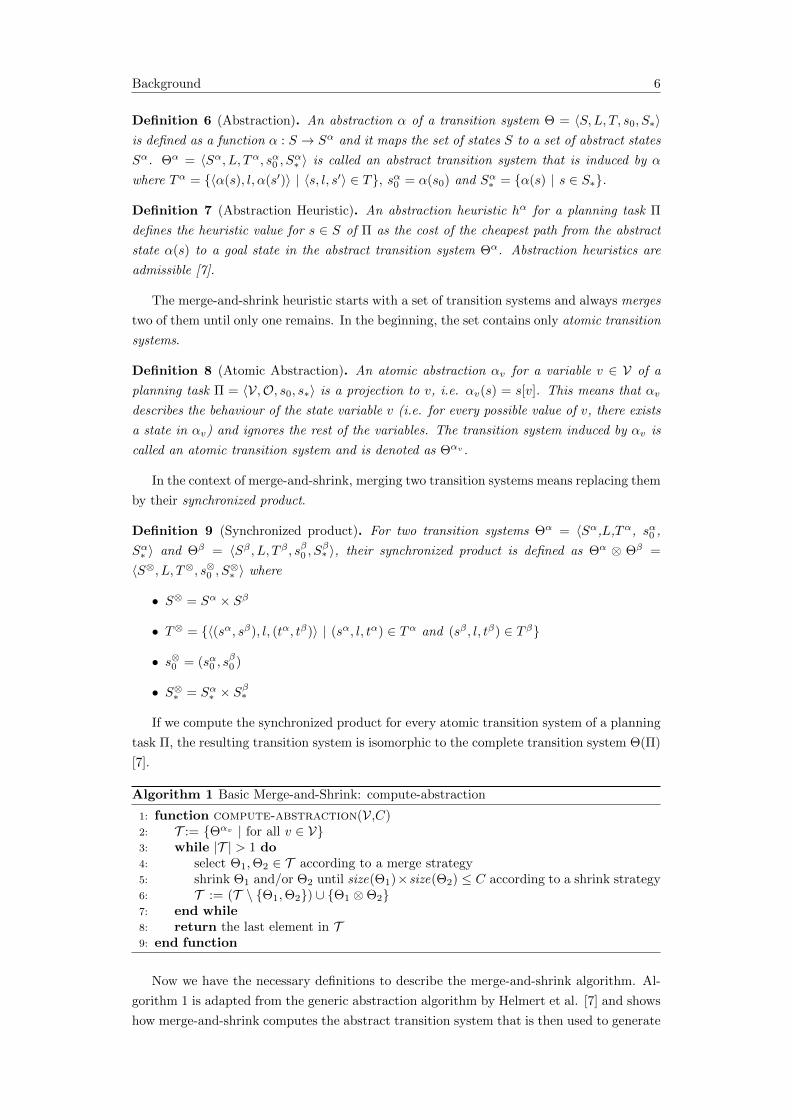
Definition 6 (Abstraction). An abstraction α of a transition system Θ = 〈S,L, T, s0, S∗〉is defined as a function α : S → Sα and it maps the set of states S to a set of abstract states
Sα. Θα = 〈Sα, L, Tα, sα0 , Sα∗ 〉 is called an abstract transition system that is induced by α
where Tα = {〈α(s), l, α(s′)〉 | 〈s, l, s′〉 ∈ T}, sα0 = α(s0) and Sα∗ = {α(s) | s ∈ S∗}.
Definition 7 (Abstraction Heuristic). An abstraction heuristic hα for a planning task Π
defines the heuristic value for s ∈ S of Π as the cost of the cheapest path from the abstract
state α(s) to a goal state in the abstract transition system Θα. Abstraction heuristics are
admissible [7].
The merge-and-shrink heuristic starts with a set of transition systems and always merges
two of them until only one remains. In the beginning, the set contains only atomic transition
systems.
Definition 8 (Atomic Abstraction). An atomic abstraction αv for a variable v ∈ V of a
planning task Π = 〈V,O, s0, s∗〉 is a projection to v, i.e. αv(s) = s[v]. This means that αv
describes the behaviour of the state variable v (i.e. for every possible value of v, there exists
a state in αv) and ignores the rest of the variables. The transition system induced by αv is
called an atomic transition system and is denoted as Θαv .
In the context of merge-and-shrink, merging two transition systems means replacing them
by their synchronized product.
Definition 9 (Synchronized product). For two transition systems Θα = 〈Sα,L,Tα, sα0 ,
Sα∗ 〉 and Θβ = 〈Sβ , L, T β , sβ0 , Sβ∗ 〉, their synchronized product is defined as Θα ⊗ Θβ =
〈S⊗, L, T⊗, s⊗0 , S⊗∗ 〉 where
• S⊗ = Sα × Sβ
• T⊗ = {〈(sα, sβ), l, (tα, tβ)〉 | (sα, l, tα) ∈ Tα and (sβ , l, tβ) ∈ T β}
• s⊗0 = (sα0 , sβ0 )
• S⊗∗ = Sα∗ × Sβ∗
If we compute the synchronized product for every atomic transition system of a planning
task Π, the resulting transition system is isomorphic to the complete transition system Θ(Π)
[7].
Algorithm 1 Basic Merge-and-Shrink: compute-abstraction
1: function compute-abstraction(V,C)2: T := {Θαv | for all v ∈ V}3: while |T | > 1 do4: select Θ1,Θ2 ∈ T according to a merge strategy5: shrink Θ1 and/or Θ2 until size(Θ1)×size(Θ2) ≤ C according to a shrink strategy6: T := (T \ {Θ1,Θ2}) ∪ {Θ1 ⊗Θ2}7: end while8: return the last element in T9: end function
Now we have the necessary definitions to describe the merge-and-shrink algorithm. Al-
gorithm 1 is adapted from the generic abstraction algorithm by Helmert et al. [7] and shows
how merge-and-shrink computes the abstract transition system that is then used to generate
Background 7
the heuristic values for the search. The algorithm starts with a set of transition systems
T . In the beginning, this set contains an atomic transition system for every variable of the
planning task Π. The algorithm then chooses two transition system Θ1, Θ2 from T that will
be merged (i.e. replaced by their synchronized product). The merge strategy decides which
one of the transition systems in T will be selected. If the size of the synchronized product of
Θ1 and Θ2 exceeds the fixed size limit C, a shrink step will be performed: one or both of the
transition system will be shrunk, i.e. replaced by an abstraction of itself with fewer abstract
states. The shrink strategy decides how to shrink them. Then Θ1 and Θ2 will be merged, by
removing them from T and replacing them with their synchronized product Θ1 ⊗Θ2. This
step is called the merge step. These two steps are repeated until only one transition system
is left in T and the algorithm returns the remaining transition system.
An important addition to the merge-and-shrink heuristic is generalized label reduction that
was introduced by Sievers et al. [11]. The idea of label reduction is to reduce the amount
of transition labels by combining labels that have equivalent information into a single label.
Label reduction can always be performed and the labels are replaced in every transition
system of the set T . Since this thesis does not deal with label reduction, no further details
are given here.
There are many different merge strategies described in the literature. The right choice
of merge strategy can greatly improve the performance of the heuristic. For example, some
merge strategies try to merge transition systems whose resulting product can be shrunk
without losing information in order to keep the accuracy of the heuristic.
A merge strategy can be represented by a merge tree. A merge tree is a binary tree
whose leaves correspond to atomic transition systems and inner nodes represent non-atomic
transition systems. A merge strategy is called linear, if it produces a linear merge tree,
i.e. a merge tree that is a list. So for the first merge, a linear merge strategy picks two
atomic transition systems. After that, it always merges one atomic transition system and
the previously merged non-atomic transition systems. On the other hand, a non-linear
merge strategy can also merge two non-atomic transition systems together.
2.3 A Collection of Merge Strategies
In this section we give a short overview over the merge strategies and possibilities to improve
merge strategies that will be discussed in this thesis.
2.3.1 Linear Merge Strategies
Linear merge strategies are the first strategies that were used for merge-and-shrink heuristics
in classical planning. The linear merge strategy that was used by Helmert, Haslum and
Hoffmann [7] is called CGGL (causal graph/goal level). It uses information from the causal
graph [9] of the planning task Π to decide which transition systems to merge.
Definition 10 (Causal Graph). The causal graph of a planning task Π = 〈V,O, s0, s∗〉 is a
directed graph 〈V,E〉 where vertices in V correspond to the variables in V. A directed edge
from variable u to v ∈ V exists if there is an operator o = 〈pre(o), eff (o), cost(o)〉 ∈ O where
either u ∈ V (pre(o)) and v ∈ V (eff (o)) or u ∈ V (eff (o)) and v ∈ V (eff (o)) are defined.
Background 8
For the first merge, this linear merge strategy prefers atomic transition systems corre-
sponding to goal variables, i.e. variables v where v ∈ V (S∗) applies. For the remaining
merges it first tries to find variables that are connected to variables from previous merges in
the causal graph. If there are no such variables, CGGL will again search for goal variables
for merging. These conditions do not guarantee that only one variable candidate remains.
If serveral variables remain, further tie-breaking is needed.
One possible tie-breaking criteria is the variable level that can be derived from the causal
graph. The variable level is a total order, i.e. there are no ties possible. The basic idea is
that variables that have a lot of ancestors in the causal graph have a greater influence and
therefore have a higher level. The variable order implemented in the Fast Downward [6]
framework is based on variable levels.
The next linear merge strategy is called reverse level merge strategy (RL) [10]. It also
uses the variable level of the causal graph. It always merges the atomic transition system
corresponding to the variable with the highest variable level with the non-atomic transition
system or the two variables with the highest levels in the first iteration of merge-and-shrink.
In the experiments we also use the level merge strategy (L) which is simply the inverse order
of the RL merge strategy.
2.3.2 DFP
DFP is the first non-linear merge strategy that was implemented for classical planning by
Sievers, Wehrle, and Helmert [11]. It was first used for model checking [2, 3]. The basic idea
of DFP is to compute a weight for every pair of available transition systems and to choose
the pair with the lowest weight as the next merge. For the computation of the weight we
need the rank of every label of a transition system:
Definition 11 (DFP rank and weight [3]). The rank of a given label l ∈ L of a transition
system Θ with a set of transitions T is defined as rank(Θ, l) = min {h∗(s′) | 〈s, l, s′〉 ∈ T}where h∗(s) is the cost of the cheapest path from s to the nearest goal in Θ. The weight of
a pair of transition systems Θ1,Θ2 with a set of labels L1, L2 is defined as
min{max{rank(Θ1, l), rank(Θ2, l)} | l ∈ L1 ∩ L2} (2.1)
The rank of a label l is the minimum goal distance over all states that can be reached
by executing l. If the rank is low, l can be applied near a goal state. To compute the weight
for a pair of transition systems Θ1 and Θ2 we first need to compute the maximum rank of
all joint labels l of Θ1 and Θ2. The weight is then the minimum value out of these maxima
of all joint labels of Θ1 and Θ2. So the goal of DFP is to merge transition systems that have
joint labels that induce transitions near goal states.
2.3.3 MIASM
MIASM is a non-linear merge strategy that was introduced by Fan, Muller, and Holte [4].
This strategy tries to merge transition systems whose product contains a lot of unnecessary
states. A state s of a transition system is unnecessary if it is not reachable from the initial
state (i.e. there is no path from s0 to s) or if s does not have a path from s to a goal
state. Unnecessary states can be pruned without losing information. In order to find merges
Background 9
that cause unnecessary states, MIASM first performs a search for subsets of variables that
produce unnecessary states. This subset search is a best-first search in the space induced by
variable subsets. Since the search for subsets can become very time consuming, the search
will be initialised with subsets that will likely produce unnecessary states (e.g. strongly
connected components of the causal graph). A more detailed explanation of the subset search
is provided in Chapter 4. The subset search returns a set of subsets. The actual merge-
and-shrink computation needs a partition of the variable set V, i.e. a set of disjoint variable
subsets where all variables are divided into subsets. The subset search does not guarantee
disjoint variable subsets. The search for a partition in MIASM is called maximum set packing.
The found partition is then used for the merge-and-shrink computation in MIASM. It first
merges variables inside these subsets according to a WC-strategy (i.e. within a cluster) until
only one transition system for every subset remains. It then uses a BC-strategy (i.e. between
clusters) to merge the remaining transition systems until only one remains.
MIASM is a static merge strategy, which means that the complete merge tree will be
precomputed before the actual search. On the contrary, dynamic merge strategies decide
the merge during each merge-and-shrink iteration. DFP and dynamic MIASM are examples
for dynamic merge strategies.
2.3.4 Dynamic MIASM
Dynamic MIASM [12] is a simple implementation that has the same goal as MIASM. The goal
is to find merges that produce many unnecessary states in the resulting merged transition
system. Similar to the weight of DFP, dynamic MIASM (or DYN-MIASM ) computes a
score for every possible pair of transition systems. The score in DYN-MIASM consists
of the percentage of unnecessary states in the product that can be pruned immediately. In
order to compute these scores, every product needs to be computed to count the unnecessary
states. The merge strategy chooses the pair of transition systems with the highest score.
2.3.5 SCC-DFP
The SCC-DFP merge strategy was introduced by Sievers et al. [12]. This strategy uses,
as its name implies, strongly connected components (SCCs) of the causal graph (defined in
Definition 10) of a planning task Π.
Definition 12 (SCC). A strongly connected component of a directed graph is a set of vertices
S ⊆ V where every vertex is reachable from every other vertex of S (i.e. for any two vertices
s1, s2 ∈ S there exists a path from s1 to s2).
In general, a merge strategy using SCCs works as follows: it uses the strongly connected
components to influence the sequence of merges. The first step is to compute all the SCCs of
the causal graph of the given planning task. Then the strategy uses a basic merge strategy
to merge every atomic transition system corresponding to the variables in one SCC until
only one transition system remains. This is done for every SCC. The strategy then uses the
same basic merge strategy to merge the remaining transition systems. Sievers et al. use
DFP as basic merge strategy. In this thesis we also evaluate different combinations that use
SCCs, for example linear merge strategies or dynamic MIASM.
Background 10
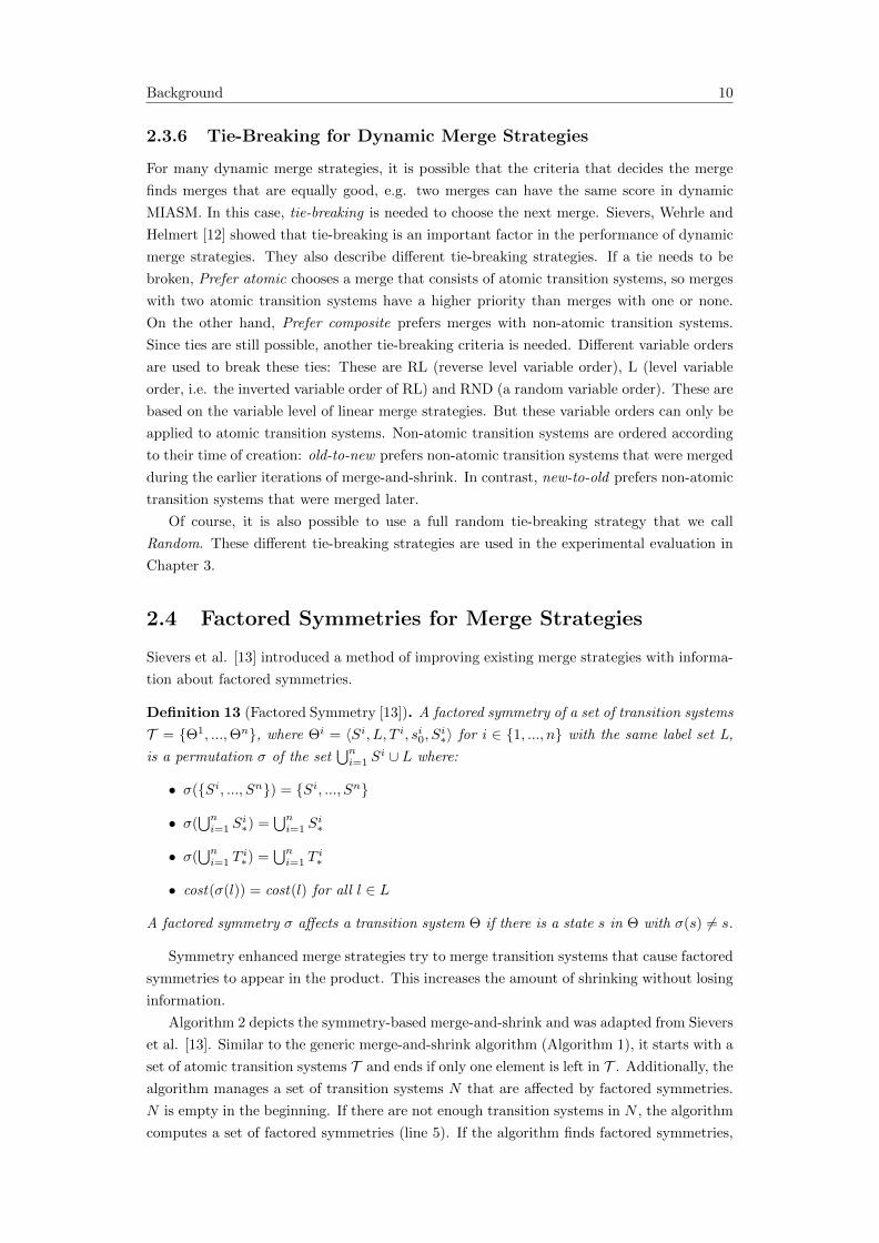
2.3.6 Tie-Breaking for Dynamic Merge Strategies
For many dynamic merge strategies, it is possible that the criteria that decides the merge
finds merges that are equally good, e.g. two merges can have the same score in dynamic
MIASM. In this case, tie-breaking is needed to choose the next merge. Sievers, Wehrle and
Helmert [12] showed that tie-breaking is an important factor in the performance of dynamic
merge strategies. They also describe different tie-breaking strategies. If a tie needs to be
broken, Prefer atomic chooses a merge that consists of atomic transition systems, so merges
with two atomic transition systems have a higher priority than merges with one or none.
On the other hand, Prefer composite prefers merges with non-atomic transition systems.
Since ties are still possible, another tie-breaking criteria is needed. Different variable orders
are used to break these ties: These are RL (reverse level variable order), L (level variable
order, i.e. the inverted variable order of RL) and RND (a random variable order). These are
based on the variable level of linear merge strategies. But these variable orders can only be
applied to atomic transition systems. Non-atomic transition systems are ordered according
to their time of creation: old-to-new prefers non-atomic transition systems that were merged
during the earlier iterations of merge-and-shrink. In contrast, new-to-old prefers non-atomic
transition systems that were merged later.
Of course, it is also possible to use a full random tie-breaking strategy that we call
Random. These different tie-breaking strategies are used in the experimental evaluation in
Chapter 3.
2.4 Factored Symmetries for Merge Strategies
Sievers et al. [13] introduced a method of improving existing merge strategies with informa-
tion about factored symmetries.
Definition 13 (Factored Symmetry [13]). A factored symmetry of a set of transition systems
T = {Θ1, ...,Θn}, where Θi = 〈Si, L, T i, si0, Si∗〉 for i ∈ {1, ..., n} with the same label set L,
is a permutation σ of the set⋃ni=1 S
i ∪ L where:
• σ({Si, ..., Sn}) = {Si, ..., Sn}
• σ(⋃ni=1 S
i∗) =
⋃ni=1 S
i∗
• σ(⋃ni=1 T
i∗) =
⋃ni=1 T
i∗
• cost(σ(l)) = cost(l) for all l ∈ L
A factored symmetry σ affects a transition system Θ if there is a state s in Θ with σ(s) 6= s.
Symmetry enhanced merge strategies try to merge transition systems that cause factored
symmetries to appear in the product. This increases the amount of shrinking without losing
information.
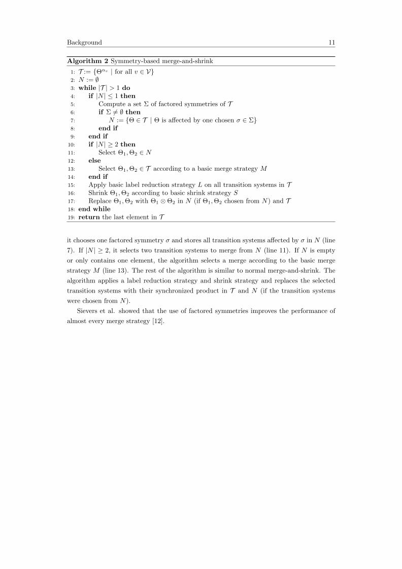
Algorithm 2 depicts the symmetry-based merge-and-shrink and was adapted from Sievers
et al. [13]. Similar to the generic merge-and-shrink algorithm (Algorithm 1), it starts with a
set of atomic transition systems T and ends if only one element is left in T . Additionally, the
algorithm manages a set of transition systems N that are affected by factored symmetries.
N is empty in the beginning. If there are not enough transition systems in N , the algorithm
computes a set of factored symmetries (line 5). If the algorithm finds factored symmetries,
Background 11
Algorithm 2 Symmetry-based merge-and-shrink
1: T := {Θαv | for all v ∈ V}2: N := ∅3: while |T | > 1 do4: if |N | ≤ 1 then5: Compute a set Σ of factored symmetries of T6: if Σ 6= ∅ then7: N := {Θ ∈ T | Θ is affected by one chosen σ ∈ Σ}8: end if9: end if
10: if |N | ≥ 2 then11: Select Θ1,Θ2 ∈ N12: else13: Select Θ1,Θ2 ∈ T according to a basic merge strategy M14: end if15: Apply basic label reduction strategy L on all transition systems in T16: Shrink Θ1,Θ2 according to basic shrink strategy S17: Replace Θ1,Θ2 with Θ1 ⊗Θ2 in N (if Θ1,Θ2 chosen from N) and T18: end while19: return the last element in T
it chooses one factored symmetry σ and stores all transition systems affected by σ in N (line
7). If |N | ≥ 2, it selects two transition systems to merge from N (line 11). If N is empty
or only contains one element, the algorithm selects a merge according to the basic merge
strategy M (line 13). The rest of the algorithm is similar to normal merge-and-shrink. The
algorithm applies a label reduction strategy and shrink strategy and replaces the selected
transition systems with their synchronized product in T and N (if the transition systems
were chosen from N).
Sievers et al. showed that the use of factored symmetries improves the performance of
almost every merge strategy [12].
3Experimental Evaluation of Merge Strategies
In this chapter we give an overview over the experimental results for various merge strategies
described in the literature. We also introduce experimental results for combinations of
existing merge strategies that have not been evaluated before. Section 3.2 gives an overview
of all evaluated merge strategies and different variations of them. Section 3.3 gives a more
detailed evaluation of DFP and DFP combined with information about factored symmetries
with different tie-breaking criteria. Section 3.4 gives an similar overview over dynamic
MIASM and also introduces a combination of dynamic MIASM with factored symmetries.
In the next section we compare the combination of dynamic MIASM with SCC to its base
strategy and to SCC with DFP.
3.1 Experimental Setup and Evaluated Attributes
All the experiments in this chapter were conducted with the existing implementation of A*
with merge-and-shrink in the Fast Downward planner [6]. The used benchmark set contains
57 different domains with a total amount of 1667 tasks to solve. Every run has a time limit
of 30 minutes and a memory limit of 2 GB. The used shrink strategy for all experiments is
the bisimulation based shrink strategy proposed by Nissim, Hoffmann and Helmert [10]. The
maximum number of states per abstraction is limited to 50000 states. In addition, exact
generalized label reduction [11] is used. We also use new-to-old ordering for non-atomic
transition systems in all experiments. The experiments were performed on a cluster of Intel
Xeon E5-2666 processors at 2.2 GHz.
We evaluate the merge strategies according to certain attributes. The coverage of a
configuration is the number of tasks that are solved within the time limit and memory limit.
The number of successful merge-and-shrink constructions is the sum of all tasks where the
construction of the merge-and-shrink heuristic is completed. If the computation exceeds
the time or memory limit it cannot construct the merge-and-shrink heuristic. The merge-
and-shrink construction time is the time that is needed to construct the heuristic. In the
experiments we use the average time out of all planning tasks. Linear order describes the
number of tasks for which the merge strategy is linear. As value we use the percentage of
tasks with linear order compared to the total number of tasks.
Experimental Evaluation of Merge Strategies 13
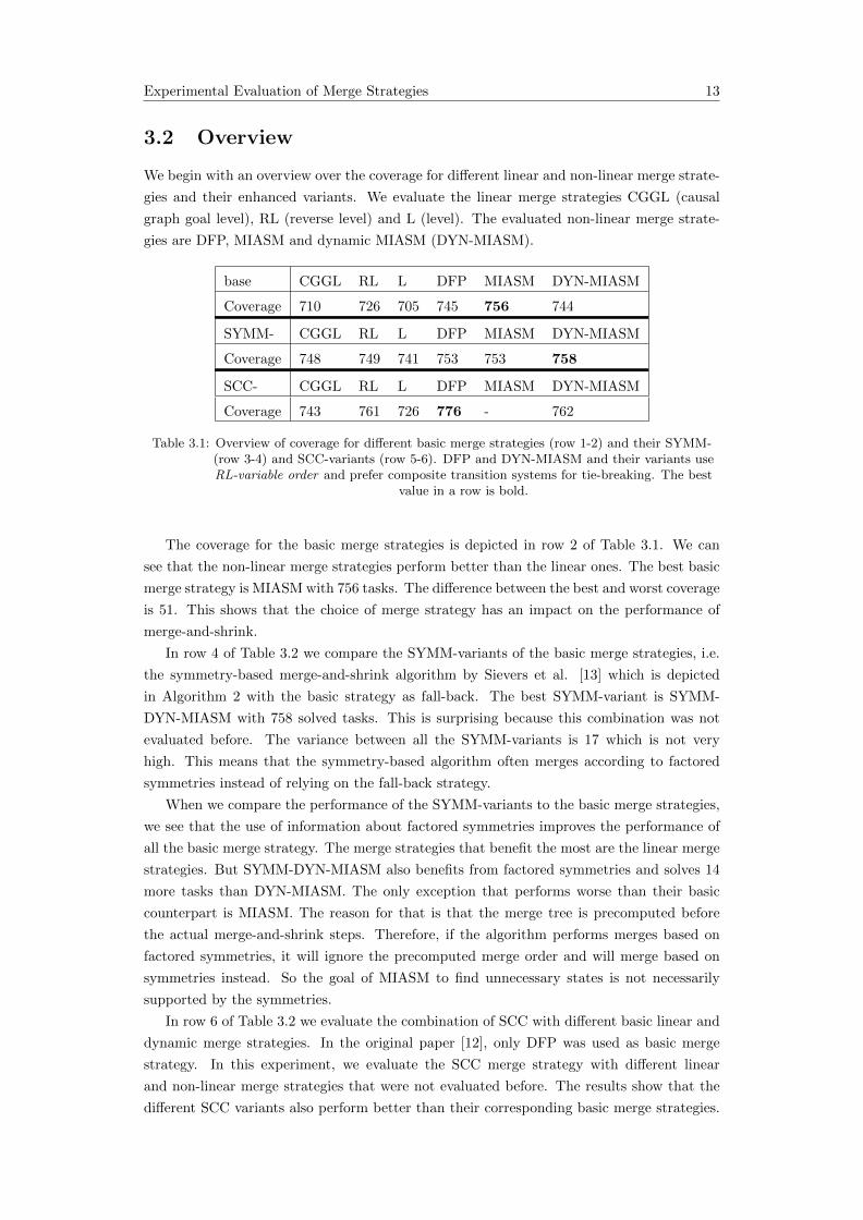
3.2 Overview
We begin with an overview over the coverage for different linear and non-linear merge strate-
gies and their enhanced variants. We evaluate the linear merge strategies CGGL (causal
graph goal level), RL (reverse level) and L (level). The evaluated non-linear merge strate-
gies are DFP, MIASM and dynamic MIASM (DYN-MIASM).
base CGGL RL L DFP MIASM DYN-MIASM
Coverage 710 726 705 745 756 744
SYMM- CGGL RL L DFP MIASM DYN-MIASM
Coverage 748 749 741 753 753 758
SCC- CGGL RL L DFP MIASM DYN-MIASM
Coverage 743 761 726 776 - 762
Table 3.1: Overview of coverage for different basic merge strategies (row 1-2) and their SYMM-(row 3-4) and SCC-variants (row 5-6). DFP and DYN-MIASM and their variants useRL-variable order and prefer composite transition systems for tie-breaking. The best
value in a row is bold.
The coverage for the basic merge strategies is depicted in row 2 of Table 3.1. We can
see that the non-linear merge strategies perform better than the linear ones. The best basic
merge strategy is MIASM with 756 tasks. The difference between the best and worst coverage
is 51. This shows that the choice of merge strategy has an impact on the performance of
merge-and-shrink.
In row 4 of Table 3.2 we compare the SYMM-variants of the basic merge strategies, i.e.
the symmetry-based merge-and-shrink algorithm by Sievers et al. [13] which is depicted
in Algorithm 2 with the basic strategy as fall-back. The best SYMM-variant is SYMM-
DYN-MIASM with 758 solved tasks. This is surprising because this combination was not
evaluated before. The variance between all the SYMM-variants is 17 which is not very
high. This means that the symmetry-based algorithm often merges according to factored
symmetries instead of relying on the fall-back strategy.
When we compare the performance of the SYMM-variants to the basic merge strategies,
we see that the use of information about factored symmetries improves the performance of
all the basic merge strategy. The merge strategies that benefit the most are the linear merge
strategies. But SYMM-DYN-MIASM also benefits from factored symmetries and solves 14
more tasks than DYN-MIASM. The only exception that performs worse than their basic
counterpart is MIASM. The reason for that is that the merge tree is precomputed before
the actual merge-and-shrink steps. Therefore, if the algorithm performs merges based on
factored symmetries, it will ignore the precomputed merge order and will merge based on
symmetries instead. So the goal of MIASM to find unnecessary states is not necessarily
supported by the symmetries.
In row 6 of Table 3.2 we evaluate the combination of SCC with different basic linear and
dynamic merge strategies. In the original paper [12], only DFP was used as basic merge
strategy. In this experiment, we evaluate the SCC merge strategy with different linear
and non-linear merge strategies that were not evaluated before. The results show that the
different SCC variants also perform better than their corresponding basic merge strategies.
Experimental Evaluation of Merge Strategies 14
The SCC variants of RL, DFP and DYN-MIASM even perform better than their symmetry
based variants. For example, the simple linear merge strategy RL with coverage of 761 and
DYN-MIASM with 762 solved tasks perform better than any basic or symmetry based merge
strategy. Still, the new evaluated SCC variants can not outperform SCC-DFP, which is the
combination that performed the best overall with 776 solved tasks.
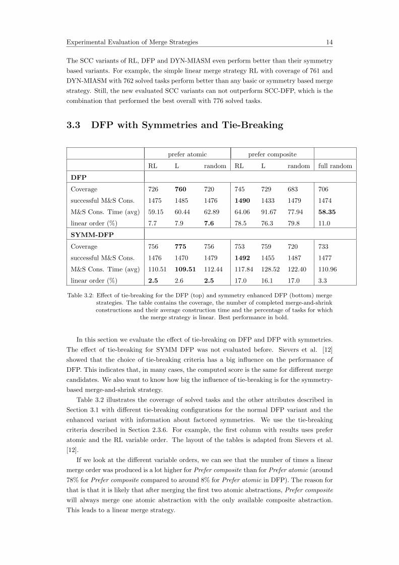
3.3 DFP with Symmetries and Tie-Breaking
prefer atomic prefer composite
RL L random RL L random full random
DFP
Coverage 726 760 720 745 729 683 706
successful M&S Cons. 1475 1485 1476 1490 1433 1479 1474
M&S Cons. Time (avg) 59.15 60.44 62.89 64.06 91.67 77.94 58.35
linear order (%) 7.7 7.9 7.6 78.5 76.3 79.8 11.0
SYMM-DFP
Coverage 756 775 756 753 759 720 733
successful M&S Cons. 1476 1470 1479 1492 1455 1487 1477
M&S Cons. Time (avg) 110.51 109.51 112.44 117.84 128.52 122.40 110.96
linear order (%) 2.5 2.6 2.5 17.0 16.1 17.0 3.3
Table 3.2: Effect of tie-breaking for the DFP (top) and symmetry enhanced DFP (bottom) mergestrategies. The table contains the coverage, the number of completed merge-and-shrinkconstructions and their average construction time and the percentage of tasks for which
the merge strategy is linear. Best performance in bold.
In this section we evaluate the effect of tie-breaking on DFP and DFP with symmetries.
The effect of tie-breaking for SYMM DFP was not evaluated before. Sievers et al. [12]
showed that the choice of tie-breaking criteria has a big influence on the performance of
DFP. This indicates that, in many cases, the computed score is the same for different merge
candidates. We also want to know how big the influence of tie-breaking is for the symmetry-
based merge-and-shrink strategy.
Table 3.2 illustrates the coverage of solved tasks and the other attributes described in
Section 3.1 with different tie-breaking configurations for the normal DFP variant and the
enhanced variant with information about factored symmetries. We use the tie-breaking
criteria described in Section 2.3.6. For example, the first column with results uses prefer
atomic and the RL variable order. The layout of the tables is adapted from Sievers et al.
[12].
If we look at the different variable orders, we can see that the number of times a linear
merge order was produced is a lot higher for Prefer composite than for Prefer atomic (around
78% for Prefer composite compared to around 8% for Prefer atomic in DFP). The reason for
that is that it is likely that after merging the first two atomic abstractions, Prefer composite
will always merge one atomic abstraction with the only available composite abstraction.
This leads to a linear merge strategy.
Experimental Evaluation of Merge Strategies 15
The results in Table 3.2 display that SYMM-DFP performs better than DFP for every
tie-breaking strategy (e.g. the coverage for prefer atomic with RL variable order is 726
for DFP and 756 for SYMM-DFP) although the number of successful merge-and-shrink
constructions is very similar between these two DFP variants (e.g. 1475 successful M&S
Constructions for DFP versus 1476 for SYMM-DFP). The average construction time for
the merge-and-shrink heuristic is also much higher for SYMM-DFP. However, SYMM-DFP
still performs better than DFP. Therefore the quality of the heuristic is better for SYMM-
DFP. In addition, the percentage of linear orders (i.e. the number of tasks where a linear
merge strategy was produced) is smaller for SYMM-DFP. For example, in 78.5 % of tasks a
linear merge strategy was computed for DFP with Prefer composite and RL variable order,
compared to 17% for SYMM-DFP.
The table also shows that the right choice of tie-breaking criteria can greatly improve
the performance of the merge-strategy for both DFP variants (difference of 77 solved tasks
between worst and best tie-breaking strategie for DFP and difference of 55 for SYMM-DFP).
It also shows that the variance of solved tasks is smaller for SYMM-DFP (i.e. 720-775 for
SYMM-DFP, 683-760 for DFP). This makes sense, because SYMM-DFP first tries to merge
according to symmetries and if no symmetries are found, it will use DFP as a fall-back
strategy. Therefore, the strategy relies less frequent on tie-breaking, because the fall-back
strategy is used less often.
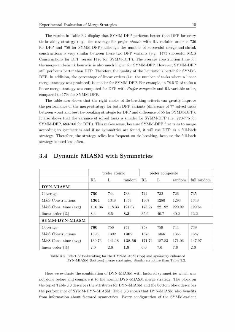
3.4 Dynamic MIASM with Symmetries
prefer atomic prefer composite
RL L random RL L random full random
DYN-MIASM
Coverage 750 744 733 744 732 726 735
M&S Constructions 1364 1348 1353 1307 1280 1293 1348
M&S Cons. time (avg) 116.35 118.33 124.67 178.27 221.92 220.92 129.64
linear order (%) 8.4 8.5 8.3 35.6 40.7 40.2 12.2
SYMM-DYN-MIASM
Coverage 760 756 747 758 759 744 739
M&S Constructions 1396 1392 1402 1373 1356 1365 1387
M&S Cons. time (avg) 139.76 141.18 138.56 171.74 187.83 171.06 147.97
linear order (%) 2.0 2.0 1.9 6.0 7.6 7.6 2.6
Table 3.3: Effect of tie-breaking for the DYN-MIASM (top) and symmetry enhancedDYN-MIASM (bottom) merge strategies. Similar structure than Table 3.2.
Here we evaluate the combination of DYN-MIASM with factored symmetries which was
not done before and compare it to the normal DYN-MIASM merge strategy. The block on
the top of Table 3.3 describes the attributes for DYN-MIASM and the bottom block describes
the performance of SYMM-DYN-MIASM. Table 3.3 shows that DYN-MIASM also benefits
from information about factored symmetries. Every configuration of the SYMM-variant
Experimental Evaluation of Merge Strategies 16
performs better than the corresponding standard configuration. Likewise, the number of
successful merge-and-shrink constructions is higher.
As seen previously in the case of DFP, the usage of information about factored symmetries
increases the average time for construction of the merge-and-shrink heuristic. For DYN-
MIASM this is also the case for Prefer atomic. On the other hand, the construction time
of the heuristic is smaller for SYMM-DYN-MIASM than DYN-MIASM with the Prefer
composite tie-breaking strategy.
The percentage of tasks where a linear merge strategy was constructed is very low for
SYMM-DYN-MIASM. In fact, SYMM-DYN-MIASM has the lowest linear order out of every
tested merge strategy, with around 2% for the Prefer atomic tie-breaking strategies and
around 6 to 7% for the Prefer composite cases.
Also, similar to Table 3.2, the variance of coverage is smaller for the SYMM-DYN-MIASM
version. In general, DYN-MIASM relies less on tie-breaking than DFP (i.e. coverage between
683 and 760 for DFP and between 726 and 750 for DYN-MIASM).
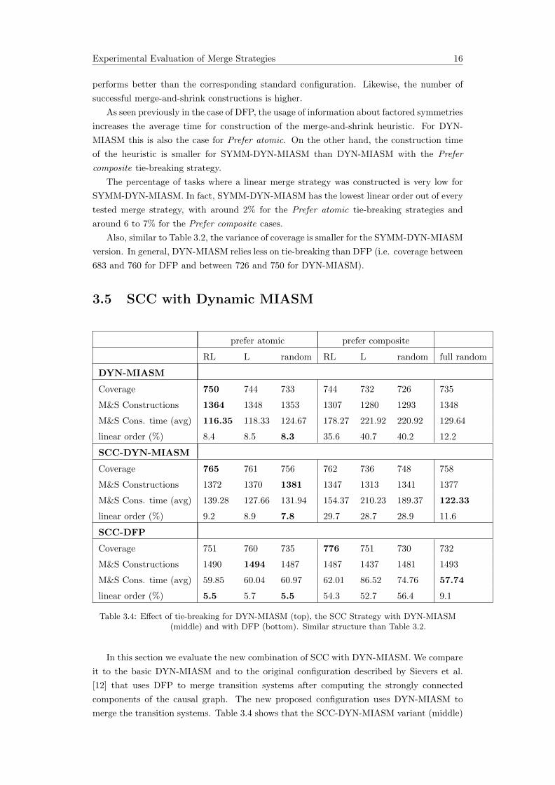
3.5 SCC with Dynamic MIASM
prefer atomic prefer composite
RL L random RL L random full random
DYN-MIASM
Coverage 750 744 733 744 732 726 735
M&S Constructions 1364 1348 1353 1307 1280 1293 1348
M&S Cons. time (avg) 116.35 118.33 124.67 178.27 221.92 220.92 129.64
linear order (%) 8.4 8.5 8.3 35.6 40.7 40.2 12.2
SCC-DYN-MIASM
Coverage 765 761 756 762 736 748 758
M&S Constructions 1372 1370 1381 1347 1313 1341 1377
M&S Cons. time (avg) 139.28 127.66 131.94 154.37 210.23 189.37 122.33
linear order (%) 9.2 8.9 7.8 29.7 28.7 28.9 11.6
SCC-DFP
Coverage 751 760 735 776 751 730 732
M&S Constructions 1490 1494 1487 1487 1437 1481 1493
M&S Cons. time (avg) 59.85 60.04 60.97 62.01 86.52 74.76 57.74
linear order (%) 5.5 5.7 5.5 54.3 52.7 56.4 9.1
Table 3.4: Effect of tie-breaking for DYN-MIASM (top), the SCC Strategy with DYN-MIASM(middle) and with DFP (bottom). Similar structure than Table 3.2.
In this section we evaluate the new combination of SCC with DYN-MIASM. We compare
it to the basic DYN-MIASM and to the original configuration described by Sievers et al.
[12] that uses DFP to merge transition systems after computing the strongly connected
components of the causal graph. The new proposed configuration uses DYN-MIASM to
merge the transition systems. Table 3.4 shows that the SCC-DYN-MIASM variant (middle)
Experimental Evaluation of Merge Strategies 17
performs better than the normal DYN-MIASM (top). Every configuration of SCC-DYN-
MIASM has a better coverage than the corresponding DYN-MIASM configuration. The
number of successful merge-and-shrink computations is also higher for SCC-DYN-MIASM
for all configuration. Merge strategies that use SCC first merge atomic transition system
that correspond to variables in a SCC. This also benefits DYN-MIASM since the merges in
this subset of variables have a higher chance of producing unnecessary states. This can lead
to more pruning.
Similar to the previous experiments, the combination relies less often on tie-breaking
than their base strategy.
The second part of Table 3.4 shows that the best DYN-MIASM variant of SCC does not
perform better than the best DFP variant (best result for SCC-DFP is 776, best result for
SCC-DYN-MIASM is 765). However, in some configurations (e.g. RL variable order and
prefer atomic), SCC-DYN-MIASM performs better than SCC-DFP. Furthermore, the vari-
ance of solved tasks is smaller for SCC-DYN-MIASM. The reason why SCC-DFP performs
better than SCC-DYN-MIASM is probably the construction time for the merge-and-shrink
heuristic: The amount of time for constructing the heuristic is in every case at least twice as
high for the variant of SCC with DYN-MIASM than the variant with DFP. This has a neg-
ative impact on the overall performance. Also, the number of successful merge-and-shrink
constructions is smaller in every case for SCC-DYN-MIASM than for SCC-DFP. This can
also be attributed to the high computation time of the heuristic for DYN-MIASM.
3.6 Conclusion
The different experiments in this section show that it is reasonable to use combinations of
merge strategies because the combinations with factored symmetries or strongly connected
components always improve the performance of the basic merge strategy for all dynamic
merge strategies. Our new evaluated combinations also perform better than their corre-
sponding merge strategies. DYN-MIASM performs better with factored symmetries and the
different strategies that use SCCs also improve their performance. However, SCC-DFP that
was described in the original paper [12] is still the best merge strategy.
We also showed that the symmetry-enhanced variants rely less on tie-breaking than their
base strategies.
4MIASM with Factored Symmetries
This chapter describes our combination of MIASM with factored symmetries. It first de-
scribes the previous implementation of MIASM with factored symmetries [13]. Then we
give a more detailed description of the subset search for MIASM. The next section describes
how this subset search was modified to use information about factored symmetries. The last
section then provides an improved implementation that finds more symmetries.
4.1 Previous Implementation of SYMM-MIASM
The previous combination of MIASM with factored symmetries uses the symmetry-based
merge-and-shrink algorithm described by Sievers et al. [13] and is depicted in Algorithm
2. This algorithm can be combined with any merge strategy and it works well for many
merge strategies: Table 3.1 in Chapter 3 shows that the merge strategies perform better if
they are enhanced with factored symmetries. Only the coverage of MIASM decreases when
using factored symmetries. The reason for this is that the merge strategy for MIASM is
static i.e. the merge tree for MIASM is built completely before the actual merge-and-shrink
computation. So if the symmetry-based merge-and-shrink finds merges according to factored
symmetries, it ignores the previously found merge order of MIASM and merges abstractions
according to factored symmetries. By destroying MIASM’s precomputed merge order, the
aim of MIASM to minimize the maximum intermediate abstraction size can also be broken.
Our approach tries to use information about factored symmetries during the precomputation
step of finding the merge order, namely in the subset search of MIASM. So we first give a
more detailed description of the subset search.
4.2 MIASM-Subset Search
The goal of MIASM is to find merges that produce unnecessary states. In order to do so,
MIASM first performs a search for subsets of variables whose merged transition systems
contain unnecessary states. This subset search is a best-first search in the space of subsets
of variables that manages a priority queue which stores the found subsets.
MIASM with Factored Symmetries 19
For the initialisation of the best-first search, the search first adds subsets that likely
produce unnecessary states to the priority queue. In the original work, this initialization
contains subsets of variables that form strongly connected components of the causal graph
and mutex groups that are provided by Fast Downward [6]. It also stores a singleton set for
every variable v ∈ V in the priority queue.
Whenever the search expands a variable subset V it adds its supersets extended with
one variable (i.e. V ∪ {v} for all v ∈ V \ V ) to the priority queue.
The subsets in the queue are ordered according to the value Rd(V ).
Definition 14 (Subset ranking [4]). The subset of variables V of the set of variables V of
a planning task Π produces unnecessary states if Rd(V ) > 0 where
Rd(V ) = minV ′⊆V
R(V ′) ∗R(V \ V ′)−R(V ) (4.1)
R(V ) is the ratio of the number of necessary states compared to the total number of states
in the combined transition system of all variables in V .
Therefore, only subsets where Rd(V ) is greater than zero are added to the priority queue.
If two subsets have the same value Rd(V ), then the smaller subset will be prioritized. It
can be very expensive to compute Rd(V ) because the search needs to perform the actual
merges for V and its subsets. This is done with a simple merge strategy called the WC-
strategy (within a cluster). This WC-strategy is also used later for the computation of
merge-and-shrink.
The search stops, if the priority queue is empty or if the total amount of states considered
in the subset search surpasses a defined limit. The subset search returns a set S that
contains subsets of variables whose product produces unnecessary states and S also contains
a singleton set for every variable v ∈ V.
4.3 Subset-Initialisation with Symmetries
The idea of our approach is to add subsets to the priority queue during the initialisation that
correspond to a set of transition systems affected by factored symmetries. So before adding
any transition system to the priority queue we first need to compute factored symmetries.
The computation for factored symmetries is done in the same way as in the symmetry-
based merge-and-shrink algorithm. We select one factored symmetry σ. There are different
possibilities for the choice of factored symmetry. For example, we can use the factored
symmetry that affects the most transition systems or the one that affects the least. After
selecting a factored symmetry σ we merge the affected atomic transition systems according
to a merge order m until only one transition system is left. These merges are done without
shrinking. The resulting non-atomic transition system is then added to the initialisation of
the subset search instead of the atomic transition systems affected by σ.
For example, we have a planning task with five atomic transition systems {Θ0, ...,Θ4}.The algorithm then finds a factored symmetry that affects Θ0,Θ1 and Θ4. It then merges
Θ0 and Θ4 resulting in Θ5 and then merges Θ1 and Θ5 to Θ6. We now only have one non-
atomic transition system left and this transition system Θ6 is added to the priority queue
alongside with Θ2 and Θ3. Now the subset search only needs to consider three transition
systems instead of five.
MIASM with Factored Symmetries 20
In order that the subset search still works we need to map the atomic transition systems
to their merged transition system. So we store a mapping for every atomic transition system
to the currently active transition system that it was merged into. So if the subset search
tries to access a transition system that was already merged, this mapping guarantees that
it accesses the merged one instead.
After the subset search and the computation of the maximum set packing, MIASM
computes the merge tree. In order to build the merge tree that can be used by merge-
and-shrink, we need to map the product of the merges according to the factored symmetry
back to its atomic transition systems. The merge order in the merge tree for the affected
transition systems in a factored symmetry σ is the same as the merge order m that was
previously used to merge the affected transition systems in σ.
4.4 Hill Climbing Search for Factored Symmetries
Our first naive approach always considers at most one factored symmetry and merges all
transition systems affected by this factored symmetry without shrinking. In some cases this
can be problematic. If we select a factored symmetry that affects many transition systems,
the product of all transition systems affected by the factored symmetry can become very
large and sometimes even exceeds the amount of available memory. The approach described
in this section tries to solve this problem by only using factored symmetries that are not too
big, so that the computation of the product of all affected transition systems is feasible. A
further improvement to our previous approach is that we now consider more than just one
factored symmetry. In order to find suitable factored symmetries that are used in the subset
search of MIASM, we perform a hill climbing search over the set of factored symmetries.
Here a factored symmetry is considered suitable if it fulfils the following criteria: the size
of the product of transition systems affected by the factored symmetry needs to be smaller
than a previously defined limit and the factored symmetry cannot affect transition systems
that are already affected by previously found factored symmetries.
Algorithm 3 Hill Climbing selection of factored symmetries
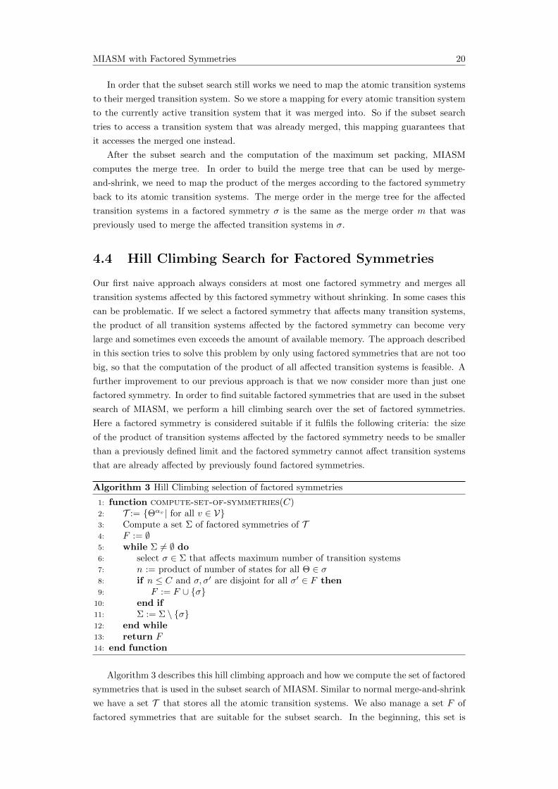
1: function compute-set-of-symmetries(C)2: T := {Θαv | for all v ∈ V}3: Compute a set Σ of factored symmetries of T4: F := ∅5: while Σ 6= ∅ do6: select σ ∈ Σ that affects maximum number of transition systems7: n := product of number of states for all Θ ∈ σ8: if n ≤ C and σ, σ′ are disjoint for all σ′ ∈ F then9: F := F ∪ {σ}
10: end if11: Σ := Σ \ {σ}12: end while13: return F14: end function
Algorithm 3 describes this hill climbing approach and how we compute the set of factored
symmetries that is used in the subset search of MIASM. Similar to normal merge-and-shrink
we have a set T that stores all the atomic transition systems. We also manage a set F of
factored symmetries that are suitable for the subset search. In the beginning, this set is
MIASM with Factored Symmetries 21
empty. We then compute the factored symmetries of T and store them in Σ. We select
the one factored symmetry σ out of Σ that affects the largest number of transition systems
(line 6). We then compute n which is the product of number of states of every transition
system in σ, i.e. the size of the synchronized product of all transition systems in σ. If n
exceeds a fixed limit C then σ is not added into F . The other criterion that must be fulfilled
in order to add a σ to F is that σ needs to be disjoint to all other factored symmetries
in F , i.e. σ cannot affect an atomic transition system that is already affected by another
factored symmetry in F . If σ meets these two criteria, it is added to F . After checking σ it
is removed from Σ. We select the next σ out of Σ and check if it is suitable until Σ is empty.
We then return the set of found factored symmetries F .
The rest of the subset search is similar to our first approach, but here we use all the
factored symmetries in F instead of only one chosen factored symmetry. So for every factored
symmetry σ in F we merge all transition systems affected by σ and initialise the subset search
as described in Section 4.3.
5Experimental Results
In this chapter, we discuss the performance of our implemented combinations of MIASM with
symmetries. We compare it to the original MIASM implementation and the old combination
of MIASM with symmetries [13].
5.1 Overview
We begin with an overview over the four versions of MIASM. We compare the original
MIASM implementation by Fan et al. [4], SYMM-MIASM based on the symmetry-based
merge-and-shrink algorithm [13], our first naive implementation with one factored symmetry
described in Chapter 4.3 (here called Naive-Combo) and our hill climbing approach (Chapter
4.4) that is called HC-Combo here. Our combinations are implemented in the Fast Downward
planner by Helmert [6]. We here use the same experimental setup as described in Chapter
3.1. In addition, for Naive-Combo, we always choose the factored symmetry that affects the
least amount of transition systems and we merge all the transition systems that are affected
by the chosen symmetry. For HC-Combo we use C = 50000 for the maximum number of
states for the product of all transition systems affected by a factored symmetry.
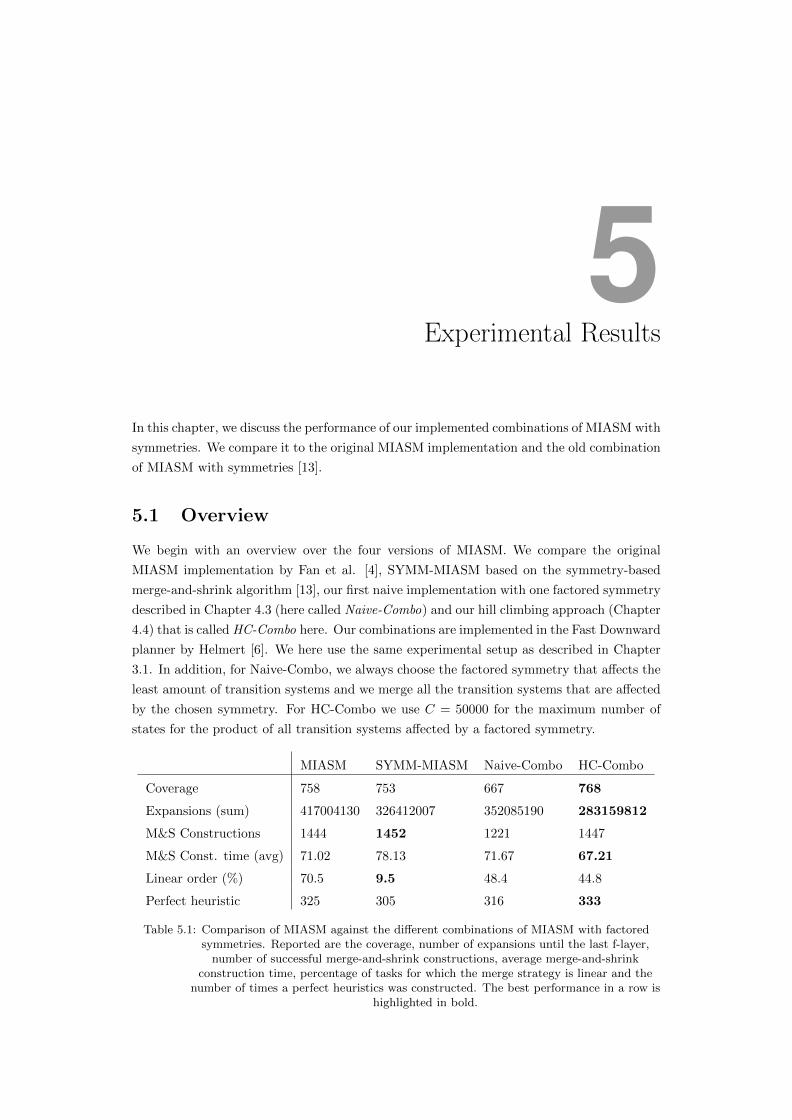
MIASM SYMM-MIASM Naive-Combo HC-Combo
Coverage 758 753 667 768
Expansions (sum) 417004130 326412007 352085190 283159812
M&S Constructions 1444 1452 1221 1447
M&S Const. time (avg) 71.02 78.13 71.67 67.21
Linear order (%) 70.5 9.5 48.4 44.8
Perfect heuristic 325 305 316 333
Table 5.1: Comparison of MIASM against the different combinations of MIASM with factoredsymmetries. Reported are the coverage, number of expansions until the last f-layer,
number of successful merge-and-shrink constructions, average merge-and-shrinkconstruction time, percentage of tasks for which the merge strategy is linear and the
number of times a perfect heuristics was constructed. The best performance in a row ishighlighted in bold.
Experimental Results 23
Table 5.1 describes the result of this experiment. First we look at the coverage: the
original MIASM solves 758 tasks. SYMM-MIASM solves less tasks (753 compared to 758
of MIASM). As described in chapter 4.1, the symmetry-based merge-and-shrink destroys
the order of the precomputed merge tree and therefore performs worse than MIASM. As
expected, Naive-Combo has the worst coverage. It only solves 667 tasks, around 100 tasks
less than HC-Combo. We can see the reason for that in the number of successfully con-
structed merge and shrink heuristics. Naive-Combo finishes around 200 merge-and-shrink
constructions less than the rest of the merge strategies. The reason why the construction
fails more often for Naive-Combo is given in Table 5.2. As expected, the merge-and-shrink
construction often runs out of memory namely around 270 times more than HC-Combo.
The problem with Naive-Combo is that it merges transition systems that are affected by
factored symmetries without shrinking. If we find a factored symmetry that affects a lot
of transition systems, the resulting merge can become very large and can exceed the mem-
ory limit. This also leads to the small amount of solved tasks. The last row in Table 5.2
shows, that Naive-Combo often hits the memory limit before reaching the time limit, since
the number of times when the merge-and-shrink construction runs out of time is smaller for
Naive-Combo than HC-Combo.
On the other hand, our HC-Combo approach solves the most tasks. With a coverage of
768 tasks, it solves 10 more tasks than the original MIASM and 15 more tasks than SYMM-
MIASM. So our HC-Combo approach outperforms the original MIASM and the previous
combination of factored symmetries with MIASM in the case of coverage. HC-Combo also
has the overall smallest number of expansions (e.g. around a third less expansions than
MIASM). We later give a more detailed overview of the domain-wise number of expansions.
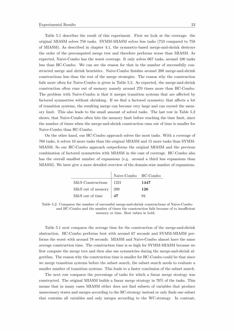
Naive-Combo HC-Combo
M&S Constructions 1221 1447
M&S out of memory 399 126
M&S out of time 47 94
Table 5.2: Compares the number of successful merge-and-shrink constructions of Naive-Comboand HC-Combo and the number of times the construction fails because of to insufficient
memory or time. Best values in bold.
Table 5.1 next compares the average time for the construction of the merge-and-shrink
abstraction. HC-Combo performs best with around 67 seconds and SYMM-MIASM per-
forms the worst with around 78 seconds. MIASM and Naive-Combo almost have the same
average construction time. The construction time is so high for SYMM-MIASM because we
first compute the merge tree and then also use symmetries during the merge-and-shrink al-
gorithm. The reason why the construction time is smaller for HC-Combo could be that since
we merge transition systems before the subset search, the subset search needs to evaluate a
smaller number of transition systems. This leads to a faster conclusion of the subset search.
The next row compares the percentage of tasks for which a linear merge strategy was
constructed. The original MIASM builds a linear merge strategy in 70% of the tasks. This
means that in many cases MIASM either does not find subsets of variables that produce
unnecessary states and merges according to the BC-strategy instead or only finds one subset
that contains all variables and only merges according to the WC-strategy. In contrast,
Experimental Results 24
SYMM-MIASM has by far the lowest amount of linear orders (around 10%). Similar to
the other SYMM-variants evaluated in Chapter 3 the amount of linear orders is very low.
So SYMM-MIASM probably often merges according to symmetries instead of using the
precomputed merge tree. The linear order of Naive-Combo and HC-Combo is almost the
same (around 45%). The number of tasks for which the merge strategy is linear is smaller
for our two approaches than for MIASM. This means that Naive-Combo and HC-Combo
often merge according to symmetries and the use of factored symmetries in the subset search
of MIASM affects the merge tree. On the other hand, the linear order of Naive-Combo and
HC-Combo is higher than for SYMM-MIASM. So due to the use of factored symmetries
in the precomputation instead of using them during the merge-and-shrink algorithm, the
merge tree gets less disrupted and focuses more on the goals of MIASM.
The number of times a perfect heuristic is constructed is highest for HC-Combo. A
perfect heuristic can be build in 333 cases.
All in all, we can see that our HC-Combo approach in general performs better than
the original MIASM and the previously implemented combination SYMM-MIASM. The
smaller amount of expansions and the smaller construction time of the abstraction leads
to a better coverage. Only Naive-Combo performs worse compared to the other variants.
That is because the construction of the abstraction often exceeds the memory limit if we
find factored symmetries that affect many transition systems.
5.2 Domain-specific evaluation
Since HC-Combo performs better than Naive-Combo, we take a closer look on the domain-
wise performance of HC-Combo.
5.2.1 MIASM against HC-Combo
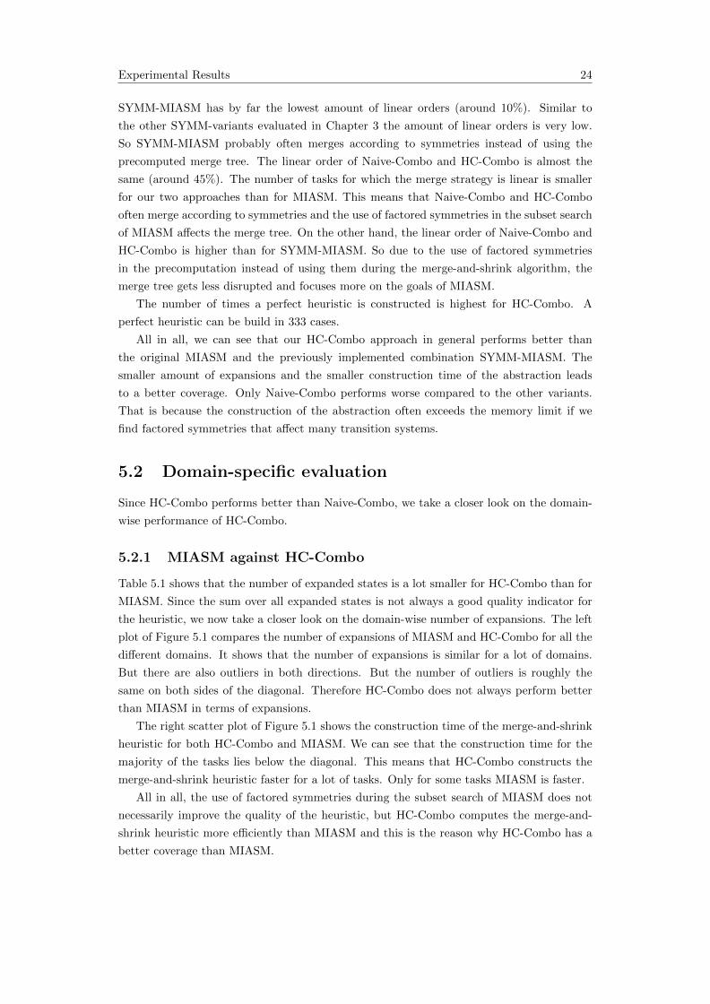
Table 5.1 shows that the number of expanded states is a lot smaller for HC-Combo than for
MIASM. Since the sum over all expanded states is not always a good quality indicator for
the heuristic, we now take a closer look on the domain-wise number of expansions. The left
plot of Figure 5.1 compares the number of expansions of MIASM and HC-Combo for all the
different domains. It shows that the number of expansions is similar for a lot of domains.
But there are also outliers in both directions. But the number of outliers is roughly the
same on both sides of the diagonal. Therefore HC-Combo does not always perform better
than MIASM in terms of expansions.
The right scatter plot of Figure 5.1 shows the construction time of the merge-and-shrink
heuristic for both HC-Combo and MIASM. We can see that the construction time for the
majority of the tasks lies below the diagonal. This means that HC-Combo constructs the
merge-and-shrink heuristic faster for a lot of tasks. Only for some tasks MIASM is faster.
All in all, the use of factored symmetries during the subset search of MIASM does not
necessarily improve the quality of the heuristic, but HC-Combo computes the merge-and-
shrink heuristic more efficiently than MIASM and this is the reason why HC-Combo has a
better coverage than MIASM.
Experimental Results 25
Figure 5.1: Shows the number of expansions until last f-layer (left) and construction time of themerge-and-shrink heuristic (right) for MIASM and HC-Combo
5.2.2 SYMM-MIASM against HC-Combo
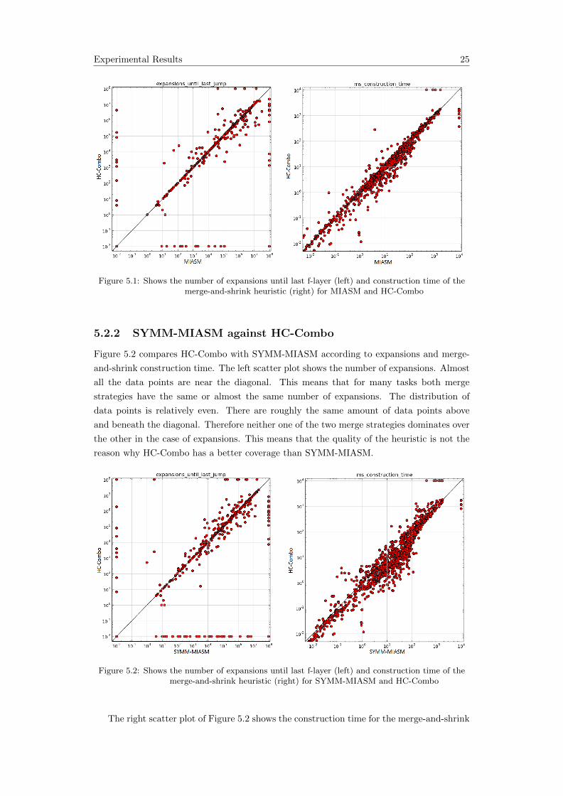
Figure 5.2 compares HC-Combo with SYMM-MIASM according to expansions and merge-
and-shrink construction time. The left scatter plot shows the number of expansions. Almost
all the data points are near the diagonal. This means that for many tasks both merge
strategies have the same or almost the same number of expansions. The distribution of
data points is relatively even. There are roughly the same amount of data points above
and beneath the diagonal. Therefore neither one of the two merge strategies dominates over
the other in the case of expansions. This means that the quality of the heuristic is not the
reason why HC-Combo has a better coverage than SYMM-MIASM.
Figure 5.2: Shows the number of expansions until last f-layer (left) and construction time of themerge-and-shrink heuristic (right) for SYMM-MIASM and HC-Combo
The right scatter plot of Figure 5.2 shows the construction time for the merge-and-shrink
Experimental Results 26
heuristic. In this plot we can see that HC-Combo is better in terms of merge-and-shrink
construction time. Considerably more data points are below the diagonal which means
HC-Combo constructs the heuristic faster than SYMM-MIASM for a lot of domains.
6Conclusion
In this thesis we showed that the combination of existing merge strategies can improve the
performance of the merge-and-shrink algorithm. We evaluated new combinations that were
not evaluated before and showed that they perform better than some original strategies, e.g.
SCC DYN-MIASM performs better than the original DYN-MIASM. We also showed that
tie-breaking is also important for the SYMM-variants of various merge strategies, although
their impact is not as high than for their original counterparts. These results show that the
merge strategy has a big impact on the performance of the merge-and-shrink heuristic. The
results also indicate that there is still a lot of room in the research of merge strategies and
it is likely that even better combinations with new improvements can be found.
Another part of this thesis was the implementation of a better combination of factored
symmetries with MIASM. We implemented two different approaches that use factored sym-
metries during the initialisation of the subset search used by MIASM. Our first approach
(Naive-Combo) does not perform very well because the size of the transition system that
is merged according to the factored symmetry exceeds the memory limit in some domains.
However, our hill climbing approach that finds factored symmetries (HC-Combo) performs
better than the original MIASM and the old combination based on the symmetry-based
merge-and-shrink [13]. It is possible that other combinations of MIASM with factored sym-
metries can still push the performance of MIASM.
Bibliography
[1] Christer Backstrom and Bernhard Nebel. Complexity results for SAS+ planning. Com-
putational Intelligence, 11(4):625–655, 1995.
[2] Klaus Drager, Bernd Finkbeiner, and Andreas Podelski. Directed model checking with
distance-preserving abstractions. In Proceedings of the the 13th International SPIN
Workshop (SPIN 2006), pages 19–34. 2006.
[3] Klaus Drager, Bernd Finkbeiner, and Andreas Podelski. Directed model checking with
distance-preserving abstractions. International Journal on Software Tools for Technol-
ogy Transfer, 11(1):27–37, 2009.
[4] Gaojian Fan, Martin Muller, and Robert Holte. Non-linear merging strategies for merge-
and-shrink based on variable interactions. In Proceedings of the Seventh Annual Sym-
posium on Combinatorial Search (SoCS 2014), pages 53–61, 2014.
[5] Peter E Hart, Nils J Nilsson, and Bertram Raphael. A formal basis for the heuristic
determination of minimum cost paths. IEEE Transactions on Systems Science and
Cybernetics, 4(2):100–107, 1968.
[6] Malte Helmert. The fast downward planning system. Journal of Artificial Intelligence
Research, 26:191–246, 2006.
[7] Malte Helmert, Patrik Haslum, and Jorg Hoffmann. Flexible abstraction heuristics for
optimal sequential planning. In Proceedings of the 17th International Conference on
Automated Planning and Scheduling (ICAPS 2007), pages 176–183, 2007.
[8] Malte Helmert, Patrik Haslum, Jorg Hoffmann, and Raz Nissim. Merge-and-shrink
abstraction: A method for generating lower bounds in factored state spaces. Journal
of the ACM, 61(3):16:1–63, 2014.
[9] Craig A Knoblock. Automatically generating abstractions for planning. Artificial In-
telligence, 68(2):243–302, 1994.
[10] Raz Nissim, Jorg Hoffmann, and Malte Helmert. Computing perfect heuristics in poly-
nomial time: On bisimulation and merge-and-shrink abstraction in optimal planning. In
Proceedings of the 22nd International Joint Conference on Artificial Intelligence (IJCAI
2011), pages 1983–1990, 2011.
[11] Silvan Sievers, Martin Wehrle, and Malte Helmert. Generalized label reduction for
merge-and-shrink heuristics. In Proceedings of the 28th AAAI Conference on Artificial
Intelligence (AAAI 2014), pages 2358–2366, 2014.
[12] Silvan Sievers, Martin Wehrle, and Malte Helmert. An analysis of merge strategies for
merge-and-shrink heuristics. In Proceedings of the 26th International Conference on
Automated Planning and Scheduling (ICAPS 2016), pages 294–298, 2016.
Bibliography 29
[13] Silvan Sievers, Martin Wehrle, Malte Helmert, Alexander Shleyfman, and Michael Katz.
Factored symmetries for merge-and-shrink abstractions. In Proceedings of the 29th
AAAI Conference on Artificial Intelligence (AAAI 2015), pages 3378–3385, 2015.