Embed Size (px)
Citation preview
MERCURY IN TURTLES FROM THE ASIAN FOOD TRADE
by
AALIYAH GREEN
(Under the Direction of J. Whitfield Gibbons and Christopher Romanek)
ABSTRACT
Mercury contamination threatens many ecosystems worldwide. Methyl mercury
bioaccumulates at each trophic level, and biomagnifies within individuals over time. Long-lived
turtles often occupy high trophic positions and are likely to accumulate mercury in contaminated
habitats. Millions of turtles worldwide are sold in Asia for human consumption. Consumers
may be at risk if turtles contain high levels of mercury. We dissected 71 turtles from 14 food
trade species and analyzed their tissues (liver, kidneys, muscle, claws, and scutes) for total
mercury content. Mercury was generally highest in carnivores, and lowest in herbivores. Liver
and scutes had the highest concentrations. We compared mercury concentrations with
consumption limits developed by the US EPA and FDA to evaluate mercury in fish tissue.
Several samples exceeded the recommended 1900 ppb consumption threshold, indicating that
consumers who eat certain turtle species frequently may be at risk for mercury-related health
problems.
INDEX WORDS: Human health, Mercury, Methylmercury, Turtles, Wildlife trade
MERCURY IN TURTLES FROM THE ASIAN FOOD TRADE
by
AALIYAH GREEN
B.S., Rutgers University, 2004
A Thesis Submitted to the Graduate Faculty of The University of Georgia in Partial Fulfillment
of the Requirements for the Degree
MASTER OF SCIENCE
ATHENS, GEORGIA
2007

© 2007
Aaliyah Green
All Rights Reserved
MERCURY IN TURTLES FROM THE ASIAN FOOD TRADE
by
AALIYAH GREEN
Major Professors: J. Whitfield Gibbons Christopher Romanek
Committee: Charles H. Jagoe
Kurt A. Buhlmann
Electronic Version Approved: Maureen Grasso Dean of the Graduate School The University of Georgia December 2007
iv
DEDICATION
To my parents, Kenneth Green and Karyn Karriem, who always encouraged me to aim high.
v
ACKNOWLEDGEMENTS
This project would not have been possible without the contributions of several colleagues at the
Savannah River Ecology Laboratory in Aiken, SC. Cris Hagen assisted in identifying and
choosing study specimens. Kurt Buhlmann created the species distribution maps. Eric Peters
and Judy Greene-McLeod advised in turtle dissection methods. The Turtle Survival Alliance and
the Tewksbury Institute of Herpetology provided the turtles. I thank Judy Greene-McLeod,
Jason Unrine, Paul Bertsch, Tracey Tuberville, Sean Poppy, and Noelle Garvin for providing
access to various lab supplies and equipment. I also thank Teresa Carroll, Lindy Steadman,
Patsy Pittman, Cherie Summer, and Melissa Mottley for administrative support. I give special
thanks to Cris Hagen and Kurt Buhlmann for contributing valuable first-hand knowledge and
expertise of exotic turtles. I am especially grateful to Heather Brant for her assistance in
mercury and stable isotope analysis and her sage advice. My committee members-- J. Whitfield
Gibbons, Christopher Romanek, Chuck Jagoe, and Kurt Buhlmann—provided priceless guidance
and support throughout my graduate studies. Lastly, I thank my family for their unconditional
love and moral support, and my boyfriend, Marcus J. Ross, for the hugs, late night pots of coffee,
and words of encouragement that helped me through this process.
vi
TABLE OF CONTENTS
Page
ACKNOWLEDGEMENTS.............................................................................................................v
LIST OF TABLES....................................................................................................................... viii
LIST OF FIGURES ....................................................................................................................... ix
INTRODUCTION ...........................................................................................................................1
Environmental Mercury Contamination in Southeast Asia.......................................1
Dietary Mercury Exposure ........................................................................................3
Physiological Effects of Mercury on Wildlife ..........................................................4
Effects of Environmental Mercury Contamination on Turtles..................................6
Asian Turtle Trade...................................................................................................12
Possible Risks to Human Consumers......................................................................13
Risk-Based Consumption Limits.............................................................................15
Purpose of Study .....................................................................................................16
METHODS ....................................................................................................................................22
Study Species ..........................................................................................................22
Turtle Acquisition....................................................................................................28
Dissection ................................................................................................................28
Sample Preparation..................................................................................................28
Analyses—Total Mercury .......................................................................................29
Analyses—Stable Isotopes ......................................................................................29
Calculation of Risk-Based Consumption Limits.....................................................30
Statistical Analyses..................................................................................................31
RESULTS .....................................................................................................................................41
vii
Mercury ...................................................................................................................41
Stable Isotopes.........................................................................................................44
Comparison of Mercury Levels to Risk-Based Consumption Limits .....................45
DISCUSSION................................................................................................................................72
Mercury ...................................................................................................................72
Stable Isotopes.........................................................................................................73
Evaluation of Risk to Human Consumers ...............................................................75
Conclusions .............................................................................................................77
REFERENCES ..............................................................................................................................80
APPENDICES ...............................................................................................................................92
A MERCURY VALUES ............................................................................................92
B STABLE ISOTOPE VALUES..............................................................................101
C TURTLE MEASUREMENTS..............................................................................109
viii
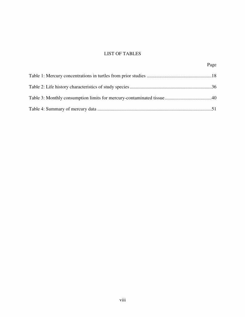
LIST OF TABLES
Page
Table 1: Mercury concentrations in turtles from prior studies ......................................................18
Table 2: Life history characteristics of study species ....................................................................36
Table 3: Monthly consumption limits for mercury-contaminated tissue.......................................40
Table 4: Summary of mercury data ...............................................................................................51
ix
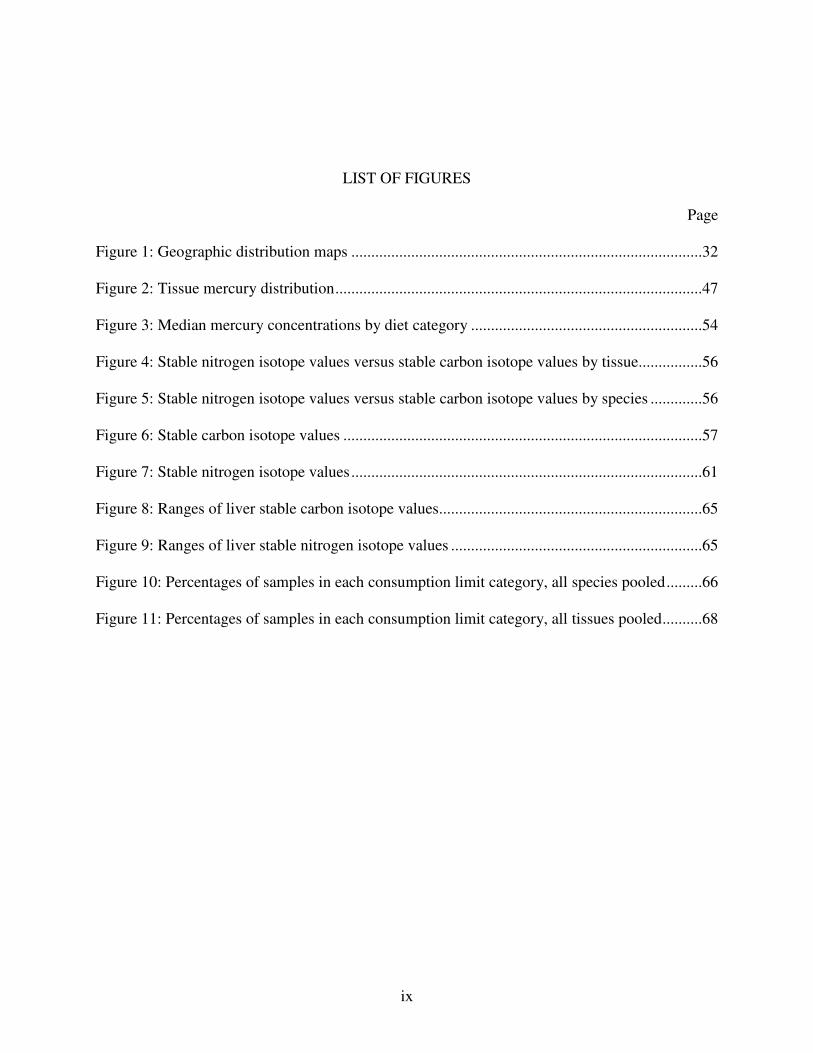
LIST OF FIGURES
Page
Figure 1: Geographic distribution maps ........................................................................................32
Figure 2: Tissue mercury distribution............................................................................................47
Figure 3: Median mercury concentrations by diet category ..........................................................54
Figure 4: Stable nitrogen isotope values versus stable carbon isotope values by tissue................56
Figure 5: Stable nitrogen isotope values versus stable carbon isotope values by species .............56
Figure 6: Stable carbon isotope values ..........................................................................................57
Figure 7: Stable nitrogen isotope values........................................................................................61
Figure 8: Ranges of liver stable carbon isotope values..................................................................65
Figure 9: Ranges of liver stable nitrogen isotope values ...............................................................65
Figure 10: Percentages of samples in each consumption limit category, all species pooled.........66
Figure 11: Percentages of samples in each consumption limit category, all tissues pooled..........68
1
INTRODUCTION
Mercury (Hg) contamination is a widespread environmental problem threatening aquatic
and terrestrial ecosystems worldwide. Coal-fired utility plants, gold and mercury mining
operations, municipal and medical waste incineration, and discharges from chlor-alkali and
cement production facilities are responsible for most of the anthropogenic load of several
hundred tons of Hg emitted globally each year (Wang et al., 2004). Almost all Hg emitted into
the atmosphere is in inorganic forms, and these are eventually deposited into lakes, rivers,
estuaries, and other bodies of water. Inorganic Hg is converted to methylmercury (MeHg) by
bacterial methylation, which adheres to sediment particles and partitions into bacteria and
plankton. From there it enters the food chain, where it biomagnifies at each successive trophic
level and bioaccumulates within organisms over time (Wang et al., 2004).
Environmental Mercury Contamination in Southeast Asia
Southeast Asia is rich in natural resources, including coal, oil, silver, gold, and other
minerals. Mining, coal production and other industrial activities, and rapid urban development
has resulted in contamination of many water systems with Hg and other pollutants.
The Guizhou Province in southern China is a major Hg and coal production center,
producing 12% of total global Hg emissions. A 2002 study found elevated Hg levels in soil, rice,
and fish in areas of the province near Hg or coal mines and industrial wastewater outputs
(Finkelman et al., 1999; Horvat et al., 2002). Xiao et al. (1998) measured Hg levels in soil and
moss on the Fanjing Mountain Nature Preserve (FMNP), a 419 km2 protected area in eastern
Guizhou Province. The area is surrounded by six large-scale Hg production centers at distances
2
of 25-200 km. Researchers found soil and moss samples at FMNP contained Hg several hundred
times higher than background levels.
Many major river systems in Southeast Asia, particularly those near crowded cities,
receive pollutant inputs from rapid urban development in addition to industrial inputs. Poor
sanitation and sewage systems in densely-populated urban centers of developing countries result
in untreated waste deposited directly into surrounding bodies of water. Zingde and Desai (1981)
estimated that India’s Thana Creek receives 56 million L/day of industrial wastewater, as well as
large quantities of domestic wastewater from nearby Mumbai. Mercury measured in water,
sediment, and zooplankton was substantially elevated compared to values measured in non-
contaminated creeks.
In the 1960s and 1970s, Thailand experienced a dramatic increase in industrial activity
and consequently, the amount of pollutants in water, soil, and seafood increased substantiallly.
Suckcharoen and Nuorteva (1978) measured Hg in fish, aquatic birds, and human hair samples
near several rivers and canals in pristine and polluted areas of Thailand. They found that Hg
concentrations in most sampled areas were among the lowest reported anywhere in the world,
with an average of 0.07 ppm (70 ppb). However, fish from the Chao Phraya estuary had highly
elevated Hg concentrations, ranging from 320 to 3,600 ppb and averaging 1,480 ppb. The
authors attribute this finding to the nearby Thai Asashi Caustic Soda Co Ltd (TACSCO) plant.
Mercury levels in wastewater from the plant averaged 900 ppb. Menasveta et al. (1985) also
documented high Hg concentrations in bivalves collected from the same area.
Gold mining is another major industry in Southeast Asia that is well known to cause
extensive regional Hg pollution. A study of the population of the Diwalwal region of Mindanao
Island, Philippines, concluded that residents had substantially elevated Hg levels in urine, blood,
and hair samples (Drasch et al., 2001). Diwalwal is home to a small-scale gold mining
3
operation, which is responsible for high amounts of Hg emitted into the local atmosphere.
Residents were exposed to atmospheric Hg and ingested Hg from contaminated fish and locally-
grown grains. Gold mines are also abundant throughout Malaysia, Papua New Guinea, and
Indonesia. These high levels of Hg in the environment are likely to negatively impact human and
wildlife populations.
Dietary Mercury Exposure
After consumption of Hg-contaminated food, Hg enters the bloodstream from the
digestive tract and is distributed to the organs within hours (Blanvillain et al., 2007). Thus, Hg
in blood represents a transient pool originating from recently-ingested food items. Total Hg
levels are usually highest in the liver, and second highest in the kidneys (Gordon et al., 1998;
Linder and Grillitsch, 2000; Sakai, 2000; Burger, 2001; Golet and Haines, 2001; Storelli and
Marcotrigiano, 2003). However, different forms of Hg accumulate to different extents in various
tissues. Inorganic Hg tends to accumulate in the kidneys (National Research Council, 2000), and
MeHg in the liver and muscles (Linder and Grillitsch, 2000; Day et al., 2005). Some studies
suggest that Hg is converted from MeHg to an inorganic form in the livers of higher vertebrates
(Albers et al., 1986; Day et al., 2005; Blanvillain et al., 2007). Therefore, proportions of
inorganic Hg and MeHg in the liver may depend to some extent on time since last meal,
individual metabolic rate, and body condition, among other factors. MeHg has a high affinity for
sulfhydryl (–SH) groups such as those present on some amino acids, and so accumulates in
protein-rich tissues like liver and muscle. Golet and Haines (2001) found that Hg levels in
muscle from the front shoulder, hind leg, and tail of snapping turtles from Connecticut were
highly correlated, indicating that Hg is evenly distributed among muscle tissues.
Keratin proteins, such as those present in scutes, are also rich in –SH functional groups,
and so tend to accumulate Hg. Various studies have used keratinous tissue, such as fur, hair,
4
claws, scutes, and feathers, to monitor Hg exposure and accumulation (Meyers-Schone and
Walton, 1994; Linder and Grillitsch, 2000). Since scutes consist of multiple layers of non-living
tissue deposited over time, they can accumulate high levels of Hg over the life of a turtle.
Several studies have reported that Hg concentrations in scutes are much higher than those in liver
and kidneys of the same animal (Sakai, 1995, 2000; Day, 2005; Blanvillain et al., 2007).
However, since most scutes are eventually shed, allocating contaminants to scutes may be an
effective mode of depuration.
Physiological Effects of Mercury on Wildlife
As awareness of the destructive impact of environmental Hg contamination has grown,
the detrimental effects of Hg have been reported in a number of studies that examined
reproduction, behavior, and physiology of birds, fish, reptiles, amphibians, and mammals.
Methylmercury’s chemical properties allow it to persist in biological tissues as well as in the
environment. Its tendency to bioaccumulate over time and biomagnify with trophic position
places long-lived predatory species at highest risk for Hg exposure (Wolfe et al., 1998; Linder
and Grillitsch, 2000). The methyl groups of the organometallic species bind readily to --SH
groups, such as those present in the amino acid cystiene. This causes MeHg to accumulate in
protein-rich tissue, such as liver, skeletal muscle, hair, feathers, and scutes.
Mercury damages the nervous system (National Research Council, 2000; Linder and
Grillitsch, 2000). Experiments with chronically-high dietary Hg levels in birds yielded
neurologic lesions, loss of muscle coordination, spinal cord degeneration, and general nervous
system dysfunction (Woebeser et al., 1976; Scheuhammer, 1988). Studies with lower to
moderate exposure levels comparable to those encountered in the field found detrimental
behavioral changes as well. Heinz (1979) observed behavioral changes in three generations of
mallards (Anas platyrhynchos) exposed to dietary Hg. Specimens were fed 500 ppb Hg in feed,
5
offered ad libitum, from nine days of age until they were euthanized as adults one year later.
Heinz reported that hens fed Hg laid a significantly greater percent (5.4% - 8.2%) of eggs outside
of the nestbox. Ducklings also had muted responses to maternal calls and were hypersensitive to
fright stimuli compared to controls. Spalding et al. (2000) reported a marked decrease in
grooming behavior in great egret nestlings (Ardea alba) that consumed 500 ppb Hg in fish ad
libitum for 14 weeks. Webber and Haines (2002) conducted a study in which golden shiners
(Notemigonus crysoleucas) were fed 500 ppb and 1,000 ppb Hg daily for 90 days. The fish
displayed drastic differences in schooling behavior and decreased predator avoidance behaviors.
These behavioral effects may make individuals more susceptible to predation, causing mercury
to pass through each trophic level at a faster rate.
Numerous studies have demonstrated reproductive effects of dietary Hg, many of which
focused on effects on birds. Common loons (Gavia immer) are large, long-lived birds that feed
almost exclusively on fish, and so can accumulate substantial tissue Hg concentrations. As a
result, they have been identified as the most important high-trophic level indicator species for Hg
pollution in North American lakes (Biodiversity Research Institute, 2005). Numerous studies
have shown that MeHg exposure has a negative impact on reproduction in loons. In a study by
Barr (1986), exposed loons laid significantly fewer eggs than loons fed non-contaminated prey.
Evers et al. (2003) conducted a field study in which 577 common loon eggs were collected from
eight states and analyzed for Hg. They found a strong inverse relationship between egg Hg
content and egg volume, suggesting that maternally-transferred Hg interferes with egg
development. Meyer et al. (1998) found similar results when they collected and tracked adult
loons and chicks from 45 lakes in Wisconsin. Reproductive success was markedly lower at lakes
where chick blood mercury levels were elevated.
6
Heinz (1979) found that mallards produced fewer viable eggs when fed 500 ppb Hg ad
libitum for one year. Shells of viable eggs were also significantly thinner than those from
unexposed hens. Chicks of exposed hens also gained significantly less weight during the first
week of life than control chicks, suggesting a developmental effect of maternally-transferred Hg.
Negative reproductive consequences of dietary Hg have also been documented in fish.
For example, Friedman et al. (1996) found that juvenile male walleye (Sander vitreus) fed
catfish containing 137 - 987 ppb of Hg three times per week for six months had significantly
impaired growth and testicular atrophy. Female juvenile fathead minnows (Pimephales
promelas) fed 80 - 850 ppb Hg from hatching to sexual maturity also displayed reduced gonadal
development, which led to a decrease in reproductive effort and spawning success
(Hammerschmidt et al., 2002).
Effects of Environmental Mercury Contamination on Turtles
Turtles have been used extensively as bioindicators of environmental contamination
(Meyers-Schone et al., 1993; Ashpole et al., 1994; Meyers-Schone and Walton, 1994; Golet and
Haines, 2001; Day et al., 2005; Bergeron et al., 2006; Blanvillain et al., 2007). Turtles have
relatively long life spans, making them well-suited for monitoring bioaccumulative pollutants
like Hg, polychlorinated biphenyls (PCBs), and organochlorine pesticides. Most freshwater and
terrestrial turtle species display site fidelity and remain within a specific home range for most of
their lives, which means contaminant levels in their tissues should closely reflect those of their
environment. Also, blood, scutes, and eggs can be sampled for contaminant analysis without
harming individual specimens or populations.
Commonly studied species:
Much research on contaminants in turtles has focused on sea turtles, common snapping
turtles (Chelydra serpentina), diamondback terrapins (Malaclemys terrapin) and sliders
7
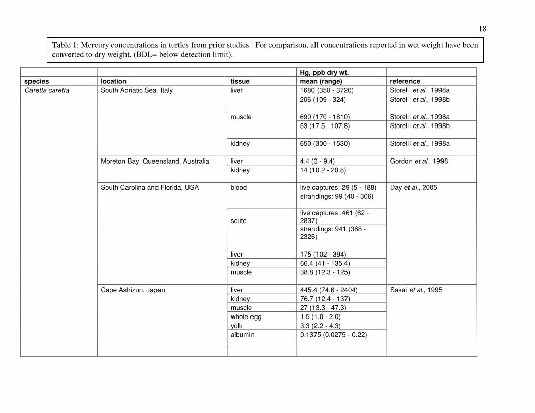
(Trachemys scripta); (Meyers-Schone and Walton, 1994). Table 1 summarizes results of prior
studies on Hg in these and other turtle species.
Common snapping turtles (C. serpentina) are large, carnivorous turtles that inhabit
freshwater and brackish environments from southern Canada to Ecuador. Their wide geographic
distribution, presence in a variety of habitats, large size, and ease of capture make them an ideal
species for monitoring contaminants in wetlands. Because of their large size, high trophic
position, and relatively long life span, they are generally expected to accumulate large amounts
of tissue Hg. Meyers-Schone et al. (1993) measured radionuclides and mercury in C. serpentina
and T. scripta from Tennessee. C. serpentina specimens had significantly higher Hg in kidneys
and muscle tissue than T. scripta specimens. Albers et al. (1986) compared Hg levels in
snapping turtles from contaminated wetlands in NJ with those from uncontaminated sites in MD.
They found that, although sediment Hg at the NJ sites was highly elevated, Hg in livers and
kidneys of snappers from these sites was relatively low. A previous study [Galuzzi (1981), as
cited by Albers et al., 1986] found a similar pattern in birds and mammals from the same areas,
suggesting that although sediment Hg concentrations were higher at the NJ sites, bioavailability
of this material was relatively low. Nonetheless, snapping turtles seem to accumulate
substantially less Hg than fish despite their size, high trophic position, and longevity, snapping
turtles seem to have substantially less Hg than fish. This may reflect an ability to allocate and
sequester contaminants in their scutes.
Diamondback terrapins (Malaclemys terrapin) are the only native US turtle that
exclusively inhabits estuarine environments. They are abundant in salt marshes and tidal creeks
along the Atlantic Coast from Massachusetts to Florida and along the Gulf Coast to Texas. This
has generated interest in using this species to monitor contamination in coastal wetlands. Burger
(2001) investigated heavy metals in tissues of terrapins from New Jersey. She found that liver
8
Hg concentrations were over 6 times higher than those in muscle tissue, averaging 1139 ppb Hg
wet wt. She concluded that consumers of terrapin livers with Hg levels similar to those
measured may be at risk due to Hg toxicity. Blanvillain et al. (2007) found that Hg
concentrations in terrapins from South Carolina differed with season. Blood Hg was
significantly lower in August than in April, June, or October.
Trophic level effects:
Diet is a major factor affecting Hg accumulation. Because Hg biomagnifies, or increases
in concentration with trophic level, turtles with more carnivorous diets tend to have higher tissue
Hg concentrations (Linder and Grillitsch, 2000; Hopkins, 2006). Anan et al. (2001) found that
adult hawksbill sea turtles (Eretmochelys imbricata), which are omnivores, had higher Hg in
livers and kidneys than herbivorous adult green turtles (Chelonia mydas) occupying the same
habitat off the coast of the Yaeyama Islands in Okinawa, Japan. Godley et al. (1999) measured
heavy metals in stranded loggerhead sea turtles (Caretta caretta) and green sea turtles from the
Mediterranean Sea. As might be expected, the carnivorous loggerhead specimens had
significantly higher Hg than the green turtles in all tissues sampled.
Ontogenetic effects:
A few studies have reported changes in tissue Hg concentrations with age. Day et al.
(2005) measured Hg in blood and scutes from 40 loggerheads captured along the coasts of South
Carolina, Georgia, and Florida. Using body mass as a proxy for age, they found a significant
increase in blood and scute Hg with mass, and suggested that there is a stable component to
blood Hg that reflects accumulated Hg from long-term exposure and which is in equilibrium with
organ Hg levels. Anan et al. (2001) measured heavy metals in 26 specimens of C. mydas and 22
specimens of E. imbricata from Okinawa, Japan. They used standard carapace length (SCL) as a
proxy for age, and found a significant positive correlation between SCL and Hg in liver and
9
kidneys. However, they also found a significant negative correlation between SCL and Hg in
muscle tissue. Similarly, Sakai et al. (2000) discovered that younger C. mydas from the same
region had higher muscle Hg than older turtles. This may be due to the dietary shift from
omnivory to herbivory that green turtles make as they age.
Sex effects:
Some studies have also reported differences in Hg distribution and accumulation between
sexes. The physiological demands of egg production might explain some variation in tissue Hg
between reproductive males and females. However, turtle eggs contain relatively small amounts
of Hg, so allocating Hg to eggs does not seem to be a major route of elimination in turtles (Sakai
et al., 1995). In contrast, Godley et al. (1999) argue that although Hg levels in individual sea
turtle eggs are very low, clutch sizes are very large and multiple clutches are laid within a
season, so the overall amount of Hg eliminated through egg laying in a single season may be
significant. Mercury concentrations in eggs may also increase with contaminant exposure.
Ashpole et al. (2004) measured contaminants in C. serpentina eggs from the St. Lawrence River
basin. Although egg Hg was relatively low at most sites (50 - 250 ppb dry wt.), eggs from the
more contaminated sites (Raquette and Turtle Rivers) averaged 720 ppb. Blanvillan (2005)
investigated the use of diamondback terrapins (Malaclemys terrapin) as biomonitors for Hg in
southeastern US estuaries. In this species, sexual dimorphism results in different dietary
preferences for males and females. Tucker et al. (1995) investigated foraging ecology of
terrapins on Kiawah Island, South Carolina, and found that the diets of terrapins with relatively
small heads (males and small- and medium-sized females) consisted of a higher proportion of
small snails than did those of terrapins with larger heads (i.e., larger females). Terrapins with
relatively large heads consumed nearly equal amounts of snails of all sizes. Larger prey items
would be expected to have correspondingly higher levels of contaminants than smaller
10
conspecifics in the same habitat. Since larger snails (with presumably higher Hg) are consumed
almost exclusively by large females, it is possible that this group of terrapins is exposed to higher
dietary mercury concentrations than males and smaller females.
Physiological effects:
It is difficult to isolate one specific contaminant (e.g., Hg) as the cause of any
physiological response seen in the field, because contaminated environments usually contain
more than one pollutant. Environmental toxicants can interact with one another, and individuals
can experience a combination of contaminant stresses. Nevertheless, a few studies have
attempted to examine physiological effects of mercury contamination on turtles. Blanvillain et
al. (2007) found a significant negative correlation between blood Hg and plasma lysozyme
activity (a common measurement of immunity) in terrapins, suggesting elevated Hg levels in
blood can result in decreased immune function. Meyers-Schone et al. (1993) documented a
higher incidence of DNA strand breakage in liver tissue of snapping turtles and sliders from a
highly contaminated site that contained Hg compared to turtles from a reference site. However,
the contaminated location they studied also had elevated levels of radionuclides, so it is unclear
what proportion of the strand breakage can be attributed to Hg. Albers et al. (1986) reported that
male snapping turtles at contaminated sites were significantly smaller than males of the same age
from uncontaminated sites. Blanvillain et al. (2007) also reported that female terrapins from a
contaminated site weighed significantly less than females collected from other sites, suggesting
that contaminant stress may contribute to decreased growth rates.
Population effects:
Effects of habitat contamination on entire populations have been observed in several
species, but have rarely been quantified. It seems that certain species may be more tolerant of
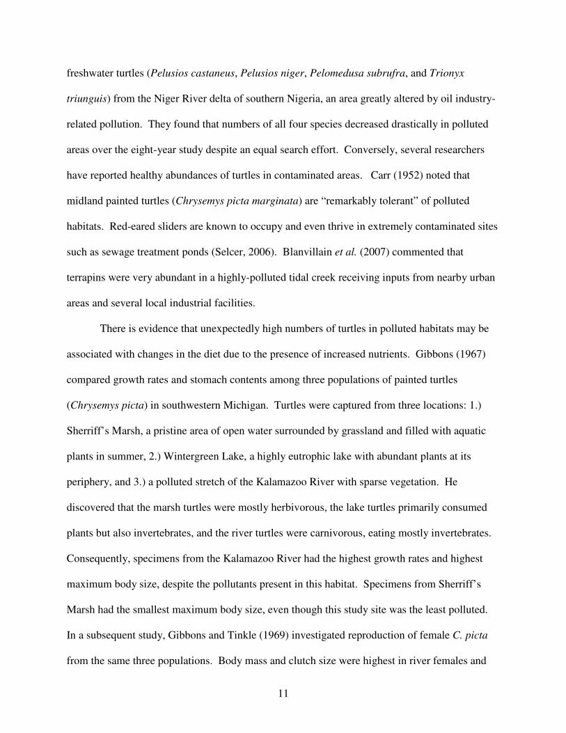
contamination than others. Luiselli et al. (2006) examined habitat use in four species of native
11
freshwater turtles (Pelusios castaneus, Pelusios niger, Pelomedusa subrufra, and Trionyx
triunguis) from the Niger River delta of southern Nigeria, an area greatly altered by oil industry-
related pollution. They found that numbers of all four species decreased drastically in polluted
areas over the eight-year study despite an equal search effort. Conversely, several researchers
have reported healthy abundances of turtles in contaminated areas. Carr (1952) noted that
midland painted turtles (Chrysemys picta marginata) are “remarkably tolerant” of polluted
habitats. Red-eared sliders are known to occupy and even thrive in extremely contaminated sites
such as sewage treatment ponds (Selcer, 2006). Blanvillain et al. (2007) commented that
terrapins were very abundant in a highly-polluted tidal creek receiving inputs from nearby urban
areas and several local industrial facilities.
There is evidence that unexpectedly high numbers of turtles in polluted habitats may be
associated with changes in the diet due to the presence of increased nutrients. Gibbons (1967)
compared growth rates and stomach contents among three populations of painted turtles
(Chrysemys picta) in southwestern Michigan. Turtles were captured from three locations: 1.)
Sherriff’s Marsh, a pristine area of open water surrounded by grassland and filled with aquatic
plants in summer, 2.) Wintergreen Lake, a highly eutrophic lake with abundant plants at its
periphery, and 3.) a polluted stretch of the Kalamazoo River with sparse vegetation. He
discovered that the marsh turtles were mostly herbivorous, the lake turtles primarily consumed
plants but also invertebrates, and the river turtles were carnivorous, eating mostly invertebrates.
Consequently, specimens from the Kalamazoo River had the highest growth rates and highest
maximum body size, despite the pollutants present in this habitat. Specimens from Sherriff’s
Marsh had the smallest maximum body size, even though this study site was the least polluted.
In a subsequent study, Gibbons and Tinkle (1969) investigated reproduction of female C. picta
from the same three populations. Body mass and clutch size were highest in river females and
12
lowest in marsh females. They concluded that differences in food quality between the three
locations was likely responsible for the observed differences in growth rate, and possibly for the
corresponding disparity in clutch size among the three populations. Although it was not
discussed in either study, it is probable that the differences in C. picta’s prey base between the
three locations resulted from high levels of nutrient pollution in the Kalamazoo River, and to a
lesser extent in Wintergreen Lake.
Asian Turtle Trade
The largest and most urgent threat to turtle populations worldwide is the unregulated food
trade based in China and Southeast Asia (Altherr and Freyer, 2000; Turtle Conservation Fund,
2002). Annually, more than 10 million turtles from around the world are sold in markets for
consumption as food or medicine. This unsustainable trade has resulted in the dramatic decline
of turtle populations worldwide, and particularly in Asia. Turtles have been used for food and
medicine in China for centuries as it has been long believed that consuming them contributes to
longevity and wisdom (Williams, 1999). Historically, the turtle trade was relatively small and
led by locals who hunted for subsistence or trade to local restaurants. In 1989, Chinese currency
became convertible, allowing direct access to foreign markets. This led to dramatically
increased exportation of turtles from Southeast Asian countries to China (Behler, 1997; Lovich et
al., 2000).
Before this change in economic policy, the majority of turtles traded in Chinese markets
were native species. Today, as many of China’s turtles have been hunted to extinction, the
markets are dominated by species from Southeast Asia, India, Africa, and North and South
America. In 2000, experts estimated that 80% of turtles sold in Chinese markets were from other
countries (McCord, 2000). This proportion is likely larger today. Several native U.S. species are
also exported to Asian markets, including common snapping turtles (Chelydra serpentina),
13
alligator snapping turtles (Macrochelys temminckii), softshell turtles (Apalone spp.), desert and
gopher tortoises (Gopherus spp.), map turtles (Graptemys spp.), sliders (Trachemys spp.), and
diamondback terrapins (Malaclemys terrapin) (Behler, 1997; Williams, 1999; Altherr and
Freyer, 2000). Several endangered species are also traded, but are usually hidden from view to
avoid conflict with authorities. These are commonly smuggled across international borders in
packages labeled as seafood (Williams, 1999; Haitao, 2000).
As turtle populations in Southeast Asia dwindle and individuals become more difficult to
find in the wild, certain species become rarer in markets, fueling demand and raising prices. The
Chinese three-striped box turtle (Cuora trifasciata), one of the most prized species on the market
for its perceived cancer-curing properties, was reported to sell for up to $3000US each in 2000
(Behler, 1997; Altherr and Freyer, 2000). Several other Cuora spp. sold for $2000US each in
2000 (McCord, 2000). Softshell turtles are a very popular luxury food, sometimes selling for
prices six times that of lamb or chicken (TRAFFIC, 2001). Meat from rare turtles has become a
delicacy in many East Asian countries and is now consumed primarily by the elite. In a way, this
economic situation drives the trade. Many collectors in Southeast Asian “source” countries, such
as Indonesia, Malaysia, Myanmar, Vietnam, Bangladesh, Laos, and Cambodia, sell turtles they
capture to traders because they are poor and turtles are profitable. These are then exported to
more developed “consumer” countries, such as China and Japan, where they are sold to
expensive restaurants and wealthy customers at high prices (Asian Turtle Working Group, 1999;
Behler, 1997; Haitao, 2004).
Possible Risks to Human Consumers
The trade in wild turtles for food and medicine is not regulated by any government
agency. These turtles are not subject to rules restricting sale of food items that contain
contaminant levels above a threshold considered safe for human consumption. It is reasonable to
14
assume that turtles from Hg-contaminated habitats are sold on the market. As a result, people
who consume turtles may be at risk of health consequences associated with elevated Hg
exposure. Frequent consumers and pregnant women would be expected to be at greatest risk.
Acute and chronic Hg exposure can cause a myriad of health problems in humans. In the
US, consumption of contaminated fish is the major source of human exposure to Hg (National
Research Council, 2000). In 2000, the National Research Council concluded that although the
risk of adverse effects from consuming tainted fish is low for the majority of the US population,
sensitive subgroups, like frequent seafood consumers, may be at greater risk. The population at
highest risk is children of women who ate large amounts of fish during pregnancy. The
developing fetus is most sensitive to mercury’s adverse effects at much lower doses than in
adults (Linder and Grillitsch, 2000; National Research Council, 2000; Schober et al., 2003).
The developing human nervous system is sensitive to Hg, which interferes with growth
and migration of neurons, creating the potential for irreversible central nervous system damage.
Chronic, low-level prenatal exposure to Hg in the maternal diet has been associated with subtle
endpoints of neurotoxicity, such as poor performance on tests of attention, fine motor function,
language, visual-spatial abilities, and verbal memory. Kjellstrom et al. (1986) studied a coastal
New Zealand population with a high rate of fish consumption. They administered tests of mental
development, motor development, and cognitive skills to children four to six years of age whose
mothers reported eating fish during pregnancy. Children exposed to moderate to high Hg levels
in utero (defined as maternal hair concentrations >6 ppm) performed significantly poorer on tests
than did children exposed to lower levels. Grandjean et al. (1997) found similar results in
children from the Faroe Islands of Denmark, where fish and whales are an important part of the
diet. Researchers followed a cohort of children born in 1986 and 1987. They characterized
exposure by measuring Hg in umbilical cord blood, maternal hair samples at partuition, and in
15
child hair samples at 12 months and seven years of age. Neuropsychological tests of seven year-
olds revealed numerous dose-related dysfunctions, most notably in language, attention, and
memory.
Risk-Based Consumption Limits
As environmental mercury contamination has become a larger and more widespread
problem in the United States in recent years, the US Environmental Protection Agency (EPA)
and Food and Drug Administration (FDA) have collaborated to develop fish consumption
advisories for the general public. Since children and pregnant and nursing women are most
susceptible to the harmful effects of dietary mercury, the EPA and FDA have recommended that
these sensitive subgroups completely avoid fish with tissue concentrations above 1 ppm (1000
ppb). This is also the FDA threshold above which fish are ineligible for interstate commerce.
The EPA has determined a reference dose for mercury of 1x10⁻⁴ mg/kg/day (ppm/day).
A reference dose is defined as “an estimate (with uncertainty spanning perhaps an order of
magnitude) of a daily exposure to a human population (including sensitive subgroups) that is
likely to be without an appreciable risk of deleterious health effects during a lifetime” (EPA,
2001). To avoid exceeding this reference dose, the EPA has recommended that humans (other
than the sensitive subgroups discussed above) do not consume fish with tissue Hg concentrations
above 1900 ppb.
Monthly consumption limits have been set for tissues with concentrations below the 1900
ppb threshold. These limits are based on tissue Hg concentration and standard estimates of meal
size and consumer body weight. Daily consumption limits are calculated using equation 1:
(1) CRlim = (RfD x BW)/Cm
Where CRlim = Maximum allowable consumption rate (kg/day)
RfD = Reference dose (1x10⁻⁴ mg/kg/day for Hg)
16
BW = Consumer body weight (kg)
Cm = Hg tissue concentration (mg/kg)
From this, the monthly consumption limit can be calculated using equation 2:
(2) CRmm = (CRlim x Tap)/MS
Where CRmm = Maximum allowable consumption rate (meals/month)
Tap = Time averaging period (365.25 days/12 months = 30.44 days/month)
MS = Meal size (kg)
Although these terms were developed for evaluating fish tissue, they will be used here to
understand potential human health risks from the consumption of Hg-contaminated turtle meat.
Purpose of Study
The primary goals of this study are to measure concentrations of Hg found in several
turtle species sold for human consumption in Asian food markets, compare Hg distribution and
accumulation patterns observed with those of more frequently studied turtle species, and
examine the relationship between tissue stable carbon and nitrogen isotope values and tissue Hg
levels to better understand the potential sources of Hg that are acquired from the diet. From this
information, species at risk may be identified, and patterns of Hg exposure may be related to
various aspects of life history characteristics and ecology, such as habitat, body size, and trophic
position. Specimens were acquired from seized shipments of turtles destined for food or pet
markets. Seventy-one deceased individuals, representing 14 species and six families from four
continents, were dissected and their tissues analyzed for mercury content and stable carbon and
nitrogen isotope content. It is hypothesized that the highest mercury levels will be measured in
turtles that are larger, older, and more carnivorous than smaller herbivorous species.
Tissue Hg levels will also be compared with Hg thresholds and guidelines established by
the EPA and the FDA to determine if Hg concentrations measured in some turtles are high
17
enough to put consumers at risk for health problems related to dietary Hg exposure. If turtles
traded in food markets contain Hg concentrations high enough to cause risk to consumers,
education and awareness of the issue may devalue certain species, relaxing pressure on
populations at risk.
18
Hg, ppb dry wt.
species location tissue mean (range) reference
Caretta caretta South Adriatic Sea, Italy liver 1680 (350 - 3720) Storelli et al., 1998a
206 (109 - 324) Storelli et al., 1998b
muscle 690 (170 - 1810) Storelli et al., 1998a
53 (17.5 - 107.8) Storelli et al., 1998b
kidney 650 (300 - 1530) Storelli et al., 1998a
Moreton Bay, Queensland, Australia liver 4.4 (0 - 9.4) Gordon et al., 1998
kidney 14 (10.2 - 20.8)
South Carolina and Florida, USA blood live captures: 29 (5 - 188) Day et al., 2005
strandings: 99 (40 - 306)
scute live captures: 461 (62 - 2837)
strandings: 941 (368 - 2326)
liver 175 (102 - 394)
kidney 66.4 (41 - 135.4)
muscle 38.8 (12.3 - 125)
Cape Ashizuri, Japan liver 445.4 (74.6 - 2404) Sakai et al., 1995
kidney 76.7 (12.4 - 137)
muscle 27 (13.3 - 47.3)
whole egg 1.5 (1.0 - 2.0)
yolk 3.3 (2.2 - 4.3)
albumin 0.1375 (0.0275 - 0.22)
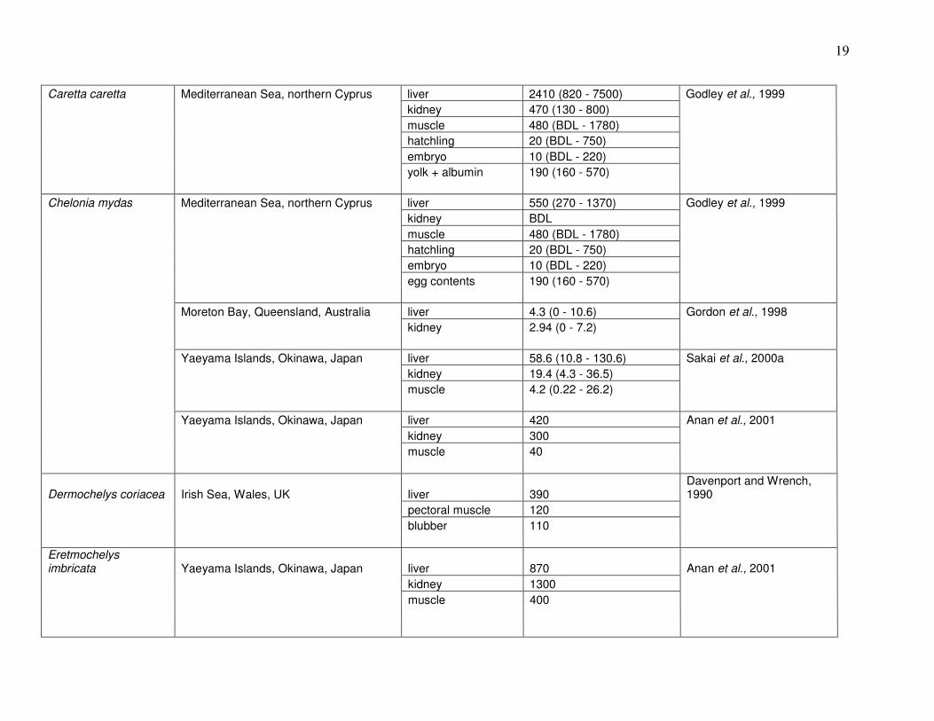
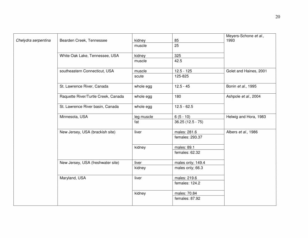
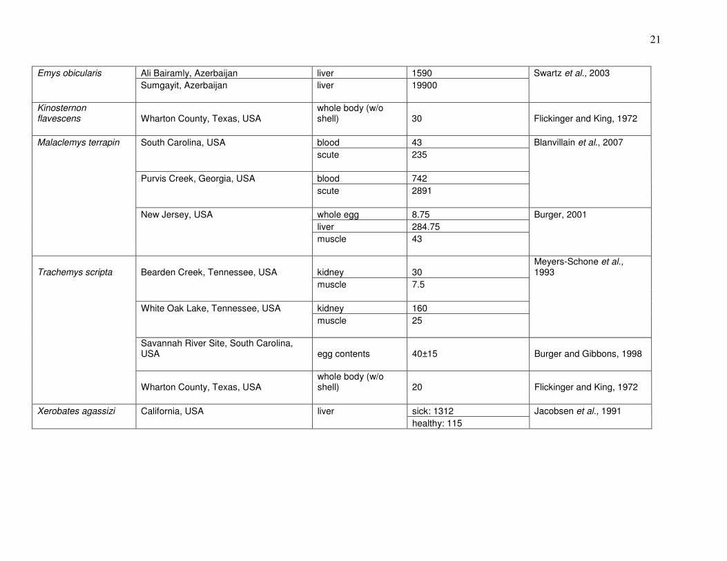
Table 1: Mercury concentrations in turtles from prior studies. For comparison, all concentrations reported in wet weight have been converted to dry weight. (BDL= below detection limit).
19
Caretta caretta Mediterranean Sea, northern Cyprus liver 2410 (820 - 7500) Godley et al., 1999
kidney 470 (130 - 800)
muscle 480 (BDL - 1780)
hatchling 20 (BDL - 750)
embryo 10 (BDL - 220)
yolk + albumin 190 (160 - 570)
Chelonia mydas Mediterranean Sea, northern Cyprus liver 550 (270 - 1370) Godley et al., 1999
kidney BDL
muscle 480 (BDL - 1780)
hatchling 20 (BDL - 750)
embryo 10 (BDL - 220)
egg contents 190 (160 - 570)
Moreton Bay, Queensland, Australia liver 4.3 (0 - 10.6) Gordon et al., 1998
kidney 2.94 (0 - 7.2)
Yaeyama Islands, Okinawa, Japan liver 58.6 (10.8 - 130.6) Sakai et al., 2000a
kidney 19.4 (4.3 - 36.5)
muscle 4.2 (0.22 - 26.2)
Yaeyama Islands, Okinawa, Japan liver 420 Anan et al., 2001
kidney 300
muscle 40
Dermochelys coriacea Irish Sea, Wales, UK liver 390 Davenport and Wrench, 1990
pectoral muscle 120
blubber 110
Eretmochelys imbricata Yaeyama Islands, Okinawa, Japan liver 870 Anan et al., 2001
kidney 1300
muscle 400
20
Chelydra serpentina Bearden Creek, Tennessee kidney 85 Meyers-Schone et al., 1993
muscle 25
White Oak Lake, Tennessee, USA kidney 325
muscle 42.5
southeastern Connecticut, USA muscle 12.5 - 125 Golet and Haines, 2001
scute 125-825
St. Lawrence River, Canada whole egg 12.5 - 45 Bonin et al., 1995
Raquette River/Turtle Creek, Canada whole egg 180 Ashpole et al., 2004
St. Lawrence River basin, Canada whole egg 12.5 - 62.5
Minnesota, USA leg muscle 6 (5 - 10) Helwig and Hora, 1983
fat 36.25 (12.5 - 75)
New Jersey, USA (brackish site) liver males: 281.6 Albers et al., 1986
females: 293.37
kidney males: 89.1
females: 62.32
New Jersey, USA (freshwater site) liver males only; 149.4
kidney males only; 66.3
Maryland, USA liver males: 219.6
females: 124.2
kidney males: 70.84
females: 87.92
21
Emys obicularis Ali Bairamly, Azerbaijan liver 1590 Swartz et al., 2003
Sumgayit, Azerbaijan liver 19900
Kinosternon flavescens Wharton County, Texas, USA
whole body (w/o shell) 30 Flickinger and King, 1972
Malaclemys terrapin South Carolina, USA blood 43 Blanvillain et al., 2007
scute 235
Purvis Creek, Georgia, USA blood 742
scute 2891
New Jersey, USA whole egg 8.75 Burger, 2001
liver 284.75
muscle 43
Trachemys scripta Bearden Creek, Tennessee, USA kidney 30 Meyers-Schone et al., 1993
muscle 7.5
White Oak Lake, Tennessee, USA kidney 160
muscle 25
Savannah River Site, South Carolina, USA egg contents 40±15 Burger and Gibbons, 1998
Wharton County, Texas, USA whole body (w/o shell) 20 Flickinger and King, 1972
Xerobates agassizi California, USA liver sick: 1312 Jacobsen et al., 1991
healthy: 115
22
METHODS
Study species
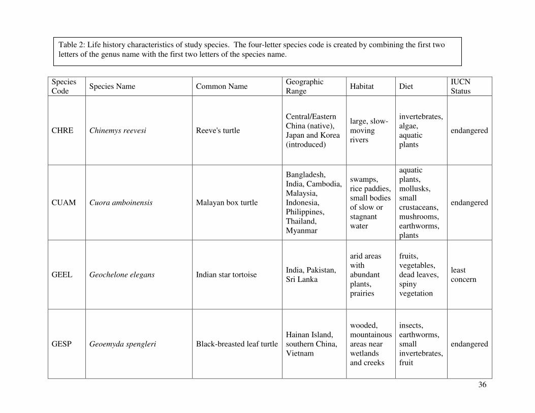
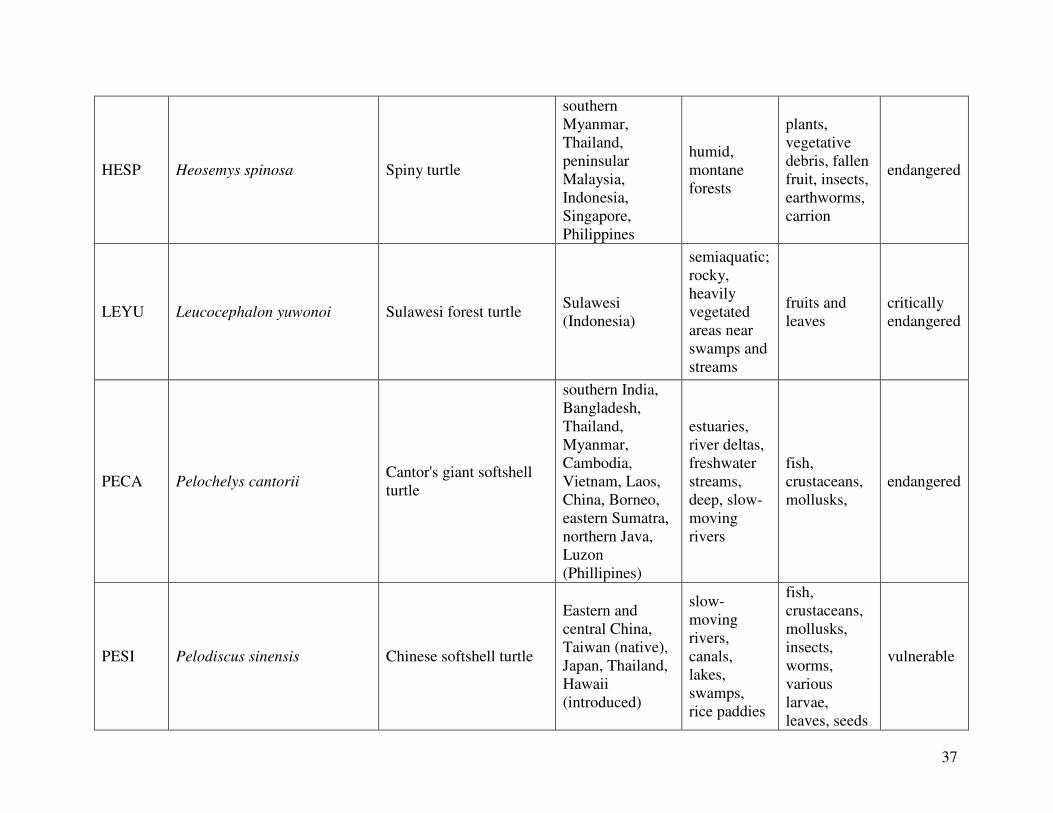
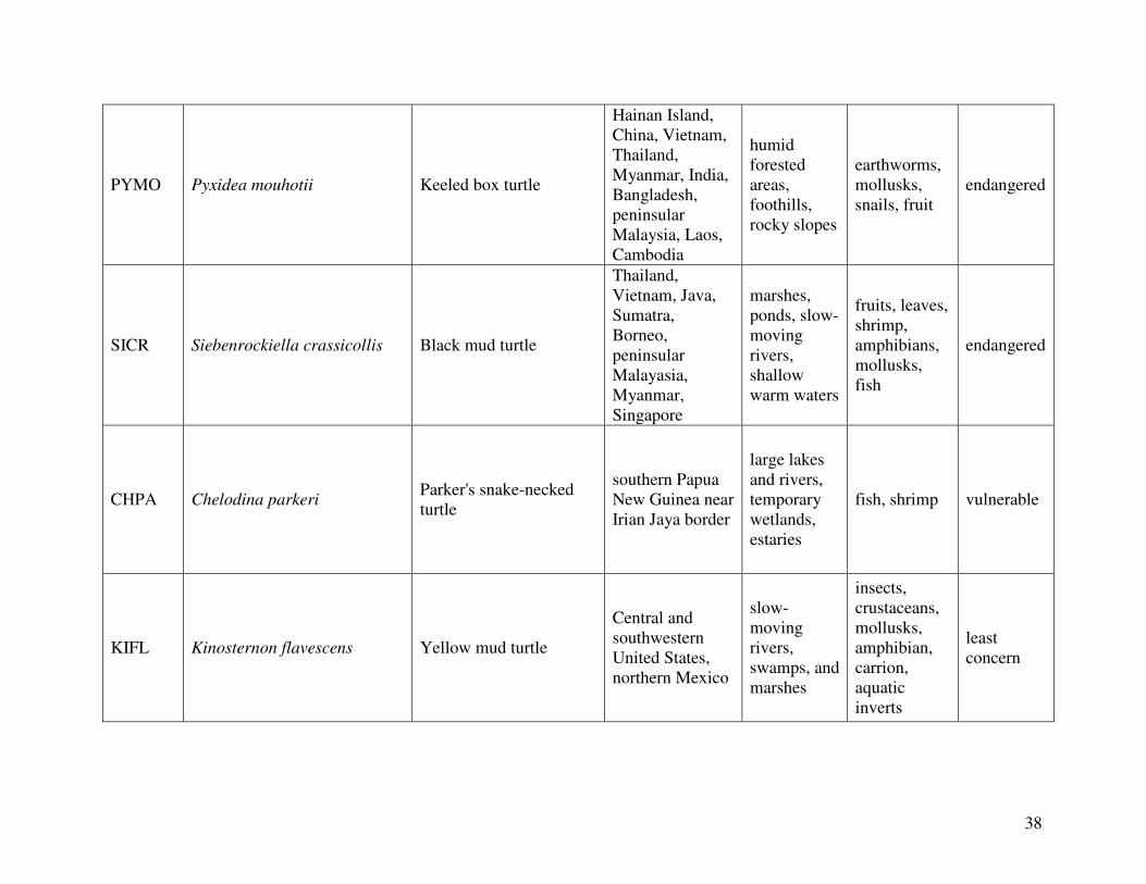
The fourteen species used in this study are described below. All status evaluations are
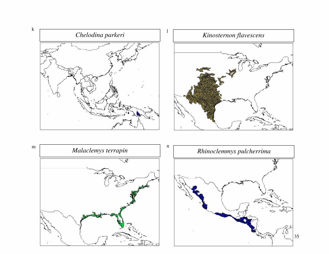
reported from the 2000 IUCN Red List. Figure 1 shows the geographical distribution of each
species. A summary the following information can be found in Table 2, which lists the diet,
habitat, geographical range, and conservation status of each species.
Reeve’s turtle (Chinemys reevesi) (n=4):
The Reeve’s turtle occurs in eastern China, Japan, Korea, Taiwan, and Hong Kong. This
small pond turtle’s carapace length (CL) does not exceed 120 mm in males and 235 mm in
females. It occupies small, shallow ponds and marshes, and can sometimes be found in large,
slow-moving rivers, basking for most of the day (Bonin et al., 2006). It has also been observed
to forage nocturnally during rains (SREL, unpubl. data). It is an omnivore, feeding on various
invertebrates, algae, and aquatic plants. This turtle was once quite popular in the food trade, but
it has become more rare as wild populations have declined in recent years. The majority of
Reeve’s turtles sold in markets today are raised on farms. This species is listed as endangered on
the IUCN’s Red List.
Malayan box turtle (Cuora amboinensis) (n=8):
The Malayan box turtle has a wide but discontinuous distribution throughout Southeast
Asia, occurring in Bangladesh, India’s Nicobar Islands, the Kaziranga National Park in Assam,
southern Myanmar, Cambodia, Malaysia, the Philippines, Sumatra, Java, and east to the
Mollucas in Indonesia. Its carapace length does not exceed 250 mm (Bonin et al., 2000). This
aquatic turtle can be found in swamps, rice paddies, and small bodies of slow or stagnant water.
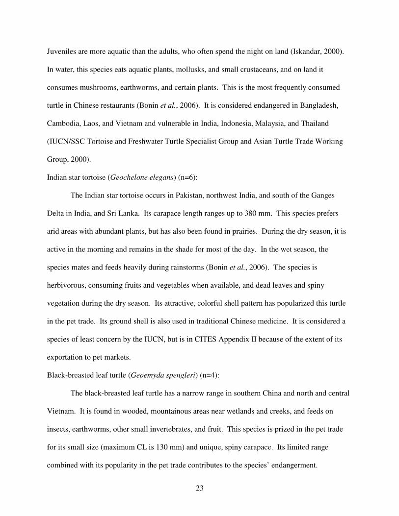
23
Juveniles are more aquatic than the adults, who often spend the night on land (Iskandar, 2000).
In water, this species eats aquatic plants, mollusks, and small crustaceans, and on land it
consumes mushrooms, earthworms, and certain plants. This is the most frequently consumed
turtle in Chinese restaurants (Bonin et al., 2006). It is considered endangered in Bangladesh,
Cambodia, Laos, and Vietnam and vulnerable in India, Indonesia, Malaysia, and Thailand
(IUCN/SSC Tortoise and Freshwater Turtle Specialist Group and Asian Turtle Trade Working
Group, 2000).
Indian star tortoise (Geochelone elegans) (n=6):
The Indian star tortoise occurs in Pakistan, northwest India, and south of the Ganges
Delta in India, and Sri Lanka. Its carapace length ranges up to 380 mm. This species prefers
arid areas with abundant plants, but has also been found in prairies. During the dry season, it is
active in the morning and remains in the shade for most of the day. In the wet season, the
species mates and feeds heavily during rainstorms (Bonin et al., 2006). The species is
herbivorous, consuming fruits and vegetables when available, and dead leaves and spiny
vegetation during the dry season. Its attractive, colorful shell pattern has popularized this turtle
in the pet trade. Its ground shell is also used in traditional Chinese medicine. It is considered a
species of least concern by the IUCN, but is in CITES Appendix II because of the extent of its
exportation to pet markets.
Black-breasted leaf turtle (Geoemyda spengleri) (n=4):
The black-breasted leaf turtle has a narrow range in southern China and north and central
Vietnam. It is found in wooded, mountainous areas near wetlands and creeks, and feeds on
insects, earthworms, other small invertebrates, and fruit. This species is prized in the pet trade
for its small size (maximum CL is 130 mm) and unique, spiny carapace. Its limited range
combined with its popularity in the pet trade contributes to the species’ endangerment.
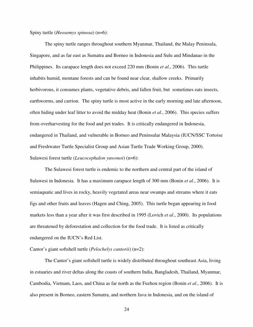
24
Spiny turtle (Heosemys spinosa) (n=6):
The spiny turtle ranges throughout southern Myanmar, Thailand, the Malay Peninsula,
Singapore, and as far east as Sumatra and Borneo in Indonesia and Sulu and Mindanao in the
Philippines. Its carapace length does not exceed 220 mm (Bonin et al., 2006). This turtle
inhabits humid, montane forests and can be found near clear, shallow creeks. Primarily
herbivorous, it consumes plants, vegetative debris, and fallen fruit, but sometimes eats insects,
earthworms, and carrion. The spiny turtle is most active in the early morning and late afternoon,
often hiding under leaf litter to avoid the midday heat (Bonin et al., 2006). This species suffers
from overharvesting for the food and pet trades. It is critically endangered in Indonesia,
endangered in Thailand, and vulnerable in Borneo and Peninsular Malaysia (IUCN/SSC Tortoise
and Freshwater Turtle Specialist Group and Asian Turtle Trade Working Group, 2000).
Sulawesi forest turtle (Leucocephalon yuwonoi) (n=6):
The Sulawesi forest turtle is endemic to the northern and central part of the island of
Sulawesi in Indonesia. It has a maximum carapace length of 300 mm (Bonin et al., 2006). It is
semiaquatic and lives in rocky, heavily vegetated areas near swamps and streams where it eats
figs and other fruits and leaves (Hagen and Ching, 2005). This turtle began appearing in food
markets less than a year after it was first described in 1995 (Lovich et al., 2000). Its populations
are threatened by deforestation and collection for the food trade. It is listed as critically
endangered on the IUCN’s Red List.
Cantor’s giant softshell turtle (Pelochelys cantorii) (n=2):
The Cantor’s giant softshell turtle is widely distributed throughout southeast Asia, living
in estuaries and river deltas along the coasts of southern India, Bangladesh, Thailand, Myanmar,
Cambodia, Vietnam, Laos, and China as far north as the Fuzhou region (Bonin et al., 2006). It is
also present in Borneo, eastern Sumatra, and northern Java in Indonesia, and on the island of
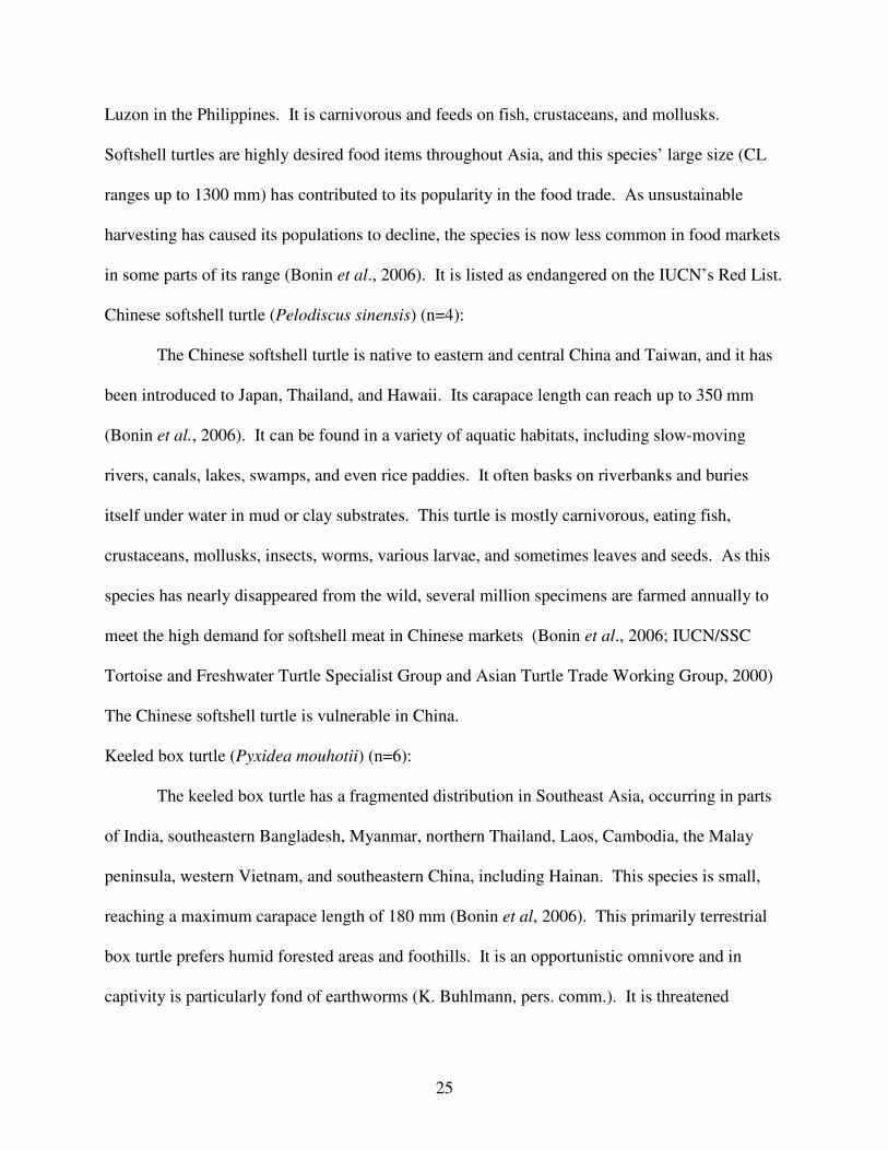
25
Luzon in the Philippines. It is carnivorous and feeds on fish, crustaceans, and mollusks.
Softshell turtles are highly desired food items throughout Asia, and this species’ large size (CL
ranges up to 1300 mm) has contributed to its popularity in the food trade. As unsustainable
harvesting has caused its populations to decline, the species is now less common in food markets
in some parts of its range (Bonin et al., 2006). It is listed as endangered on the IUCN’s Red List.
Chinese softshell turtle (Pelodiscus sinensis) (n=4):
The Chinese softshell turtle is native to eastern and central China and Taiwan, and it has
been introduced to Japan, Thailand, and Hawaii. Its carapace length can reach up to 350 mm
(Bonin et al., 2006). It can be found in a variety of aquatic habitats, including slow-moving
rivers, canals, lakes, swamps, and even rice paddies. It often basks on riverbanks and buries
itself under water in mud or clay substrates. This turtle is mostly carnivorous, eating fish,
crustaceans, mollusks, insects, worms, various larvae, and sometimes leaves and seeds. As this
species has nearly disappeared from the wild, several million specimens are farmed annually to
meet the high demand for softshell meat in Chinese markets (Bonin et al., 2006; IUCN/SSC
Tortoise and Freshwater Turtle Specialist Group and Asian Turtle Trade Working Group, 2000)
The Chinese softshell turtle is vulnerable in China.
Keeled box turtle (Pyxidea mouhotii) (n=6):
The keeled box turtle has a fragmented distribution in Southeast Asia, occurring in parts
of India, southeastern Bangladesh, Myanmar, northern Thailand, Laos, Cambodia, the Malay
peninsula, western Vietnam, and southeastern China, including Hainan. This species is small,
reaching a maximum carapace length of 180 mm (Bonin et al, 2006). This primarily terrestrial
box turtle prefers humid forested areas and foothills. It is an opportunistic omnivore and in
captivity is particularly fond of earthworms (K. Buhlmann, pers. comm.). It is threatened
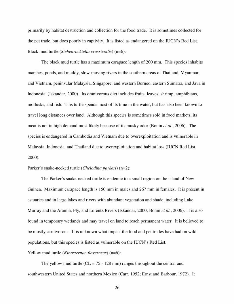
26
primarily by habitat destruction and collection for the food trade. It is sometimes collected for
the pet trade, but does poorly in captivity. It is listed as endangered on the IUCN’s Red List.
Black mud turtle (Siebenrockiella crassicollis) (n=6):
The black mud turtle has a maximum carapace length of 200 mm. This species inhabits
marshes, ponds, and muddy, slow-moving rivers in the southern areas of Thailand, Myanmar,
and Vietnam, peninsular Malaysia, Singapore, and western Borneo, eastern Sumatra, and Java in
Indonesia. (Iskandar, 2000). Its omnivorous diet includes fruits, leaves, shrimp, amphibians,
mollusks, and fish. This turtle spends most of its time in the water, but has also been known to
travel long distances over land. Although this species is sometimes sold in food markets, its
meat is not in high demand most likely because of its musky odor (Bonin et al., 2006). The
species is endangered in Cambodia and Vietnam due to overexploitation and is vulnerable in
Malaysia, Indonesia, and Thailand due to overexploitation and habitat loss (IUCN Red List,
2000).
Parker’s snake-necked turtle (Chelodina parkeri) (n=2):
The Parker’s snake-necked turtle is endemic to a small region on the island of New
Guinea. Maximum carapace length is 150 mm in males and 267 mm in females. It is present in
estuaries and in large lakes and rivers with abundant vegetation and shade, including Lake
Murray and the Aramia, Fly, and Lorentz Rivers (Iskandar, 2000; Bonin et al., 2006). It is also
found in temporary wetlands and may travel on land to reach permanent water. It is believed to
be mostly carnivorous. It is unknown what impact the food and pet trades have had on wild
populations, but this species is listed as vulnerable on the IUCN’s Red List.
Yellow mud turtle (Kinosternon flavescens) (n=6):
The yellow mud turtle (CL = 75 - 128 mm) ranges throughout the central and
southwestern United States and northern Mexico (Carr, 1952; Ernst and Barbour, 1972). It
27
occurs in slow-moving rivers, swamps, and marshes with abundant aquatic plants and muddy or
sandy bottoms. Like most mud turtles, it is an omnivore and feeds on insects, crustaceans,
mollusks, amphibians, carrion, and aquatic plants. It is not sought in the food trade, but is
occasionally found in pet markets. It is threatened by urban development, habitat alteration, and
vehicles on roads, and is considered endangered in Illinois, Iowa, and Missouri (Bonin et al.,
2006).
Diamondback terrapin (Malaclemys terrapin) (n=6):
The diamondback terrapin (CL = 100 - 140 mm in males and 150 - 230 mm in females) is
exclusive to estuarine wetlands and brackish tidal creeks along the Atlantic coast of the US from
Massachusetts to Florida and along the Gulf coast from Florida to Texas (Ernst and Barbour,
1972). Largely carnivorous, this turtle eats snails, crabs, shrimp, mollusks, other invertebrates,
small fish, carrion, and aquatic plants (Tucker et al., 1995). Its populations declined
dramatically due to overharvesting during the early 20th century when it was a popular delicacy
in the United States. Terrapin numbers have since rebounded, but the species is still threatened
by habitat destruction and alteration, road mortality of nesting females, and drowning in crab
traps (Gibbons et al., 2001) This species is still harvested in the United States and shipped to
food markets in Asia. It is protected in some eastern US states, but is considered a species of
least concern by the IUCN.
Central American wood turtle (Rhinoclemmys pulcherrima manni) (n=5):
The Central American wood turtle’s range extends from western Mexico to Costa Rica.
This subspecies occurs from southwestern Nicaragua to northern and west central Costa Rica.
Carapace length ranges up to 180 mm in males and up to 214 mm in females (Bonin et al.,
2006). It is largely terrestrial, occupying humid forested areas near streams. It is especially
active after rainfall, and may be seen swimming at pond surfaces during the dry season. Its
28
omnivorous diet consists mainly of vegetables, fruit, earthworms, insects, snails, and slugs.
Habitat destruction and automobile collisions are among the major threats to this species. This
species is generally not sought in the food trade, but is often exported to the US through the pet
trade. The IUCN considers this turtle to be a species of least concern.
Turtle acquisition
Cuora amboinensis, H. spinosa, and S. crassicollis specimens were obtained from a large
shipment of turtles that likely originated in Malaysia and was destined for food markets in China.
Customs officials in Hong Kong seized the shipment on December 11, 2001, and the Turtle
Survival Alliance (TSA) handled the distribution of live specimens to zoos, organizations, and
private individuals around the world (Hudson and Buhlmann, 2000). Several turtles were kept at
the Savannah River Ecology Laboratory (SREL) in Aiken, SC. Sick animals that subsequently
died were made available for this study. All other specimens were obtained from various
locations, including food and pet markets, and were donated to SREL by the Tewksbury Institute
of Herpetology (R. Ogust, pers. comm.) as deceased frozen specimens.
Dissection
Specimens were thawed and dissected. Portions of the liver, kidneys, pectoral muscle,
hind leg muscle, scutes, and claws were removed for analysis. In addition, follicles were
removed from female specimens when present. The dissected samples were stored individually
in sterile polyethylene Whirl-Pak® bags (NASCO) and frozen at –10 ºC until processed. Tools
were cleaned with 10% nitric acid between specimens to prevent cross-contamination.
Sample Preparation
Samples were weighed, lyophilized (Labconco), reweighed to a constant dry weight, and
then lipid extracted. Analysis for 13C/12C and 15N/14N ratios required removal of lipids (Post,
2007) through a 24 hour extraction within a 2:1 chloroform: methanol mixture followed by
29
rinsing in methanol until the decanted liquid became clear. After air drying, the extracted tissue
samples were homogenized in coffee grinders and/or a liquid nitrogen mill (Spex Sample Prep
6750 freezer mill, Metuchen, NJ, USA). Coffee grinders and freezer mill vials and stoppers
were cleaned with a metal free detergent and 10% nitric acid between samples. Aliquots of
lyophilized, homogenized, and lipid extracted tissue were then assayed for total mercury and
stable isotope content as described below.
Analyses - Total Mercury
Tissues were analyzed for Hg following EPA method 7473 (USEPA, 1998), using a
DMA80 Direct Mercury Analyzer (Milestone, Inc, Monroe, CT, USA). This method utilizes
thermal decomposition, gold amalgamation, thermal desorption and atomic absorption detection.
Samples were analyzed in batches of ten, with each batch including a blank, a sample replicate,
and a tissue standard certified for Hg concentration (DORM-2, dogfish muscle, DOLT-2 dogfish
liver, or TORT-2, lobster hepatopancreas, purchased from the National Research Council of
Canada (NRCC), Ottawa, Canada). Standard recovery ranged from 85% to 116% with an
average of 101% (n=58). The average difference between sample replicates was 2% (n=57).
Based on a 0.98 g sample and an average blank of 0.12 ng Hg (n=27), the method detection limit
(MDL) was 0.65 ppb. All samples were determined to be above the MDL. Mercury values are
based on dried and lipid-extracted tissues.
Analyses – Stable Isotopes
Elemental analysis isotope-ratio mass spectrometry (EA-IRMS) was employed to
measure the total carbon and nitrogen content, and the 13C/12C and 15N/14N ratios of individual
samples (Barrie and Prosser, 1996). Prior to isotopic analysis, approximately 1.0 - 1.5 mg of
tissue was loaded into a pre-cleaned tin capsule for weighing to ±1 µg using an ultra-
microbalance (Sartorius, Edgewood, NY, USA). Capsules were then loaded with ground
30
samples, sealed, weighed and placed into a dessicator until analyzed on a Carlo Erba Elemental
Analyzer (NC2500, Milan, Italy) attached to a continuous flow isotope ratio mass spectrometer
(Finnigan Delta plus XL; Finnigan-MAT, San Jose, CA, USA). Samples were combusted to N2
and CO2 in oxidation/reduction furnaces, separated by gas chromatography and then measured
for 13C/12C and 15N/14N ratios on the mass spectrometer. An internal N2(g) working standard was
admitted prior to the introduction of each sample and a CO2(g) standard was admitted at the
conclusion of each combustion for calibration to the AIR (nitrogen) and V-PDB (carbon)
international standards (Mariotti 1983; Coplen 1996). Stable isotope ratios are reported in per mil
units (‰) using standard delta (δ) notation (Craig 1957). External working standards of bovine
muscle, avian feather and acetanilide were analyzed to determine external precision; these
standards were reproducible to better than ±0.15‰ (1σSD) for both δ 13C and δ 15N values.
Calculation of Risk-Based Consumption Limits
To determine the maximum Hg tissue concentration that could be safely consumed in a
given time period, equation 2 was rearranged and calculated for a monthly consumption rate of
0.5, 1, 2, 3, and 4 meals per month as follows:
CRlim = (CRmm x MS)/ Tap
This maximum allowable consumption rate was then substituted into equation 1, which was
rearranged as follows:
Cm = (RfD x BW)/Clim
This gives the maximum Hg tissue concentration that can be safely consumed in one meal every
two months (1877 ppb), one meal per month (938 ppb), two meals per month (470 ppb), three
meals per month (313 ppb), and four meals per month (235 ppb). These limits were calculated
using an average US adult consumer body mass of 70 kg and an average meal size of 8 oz (0.277
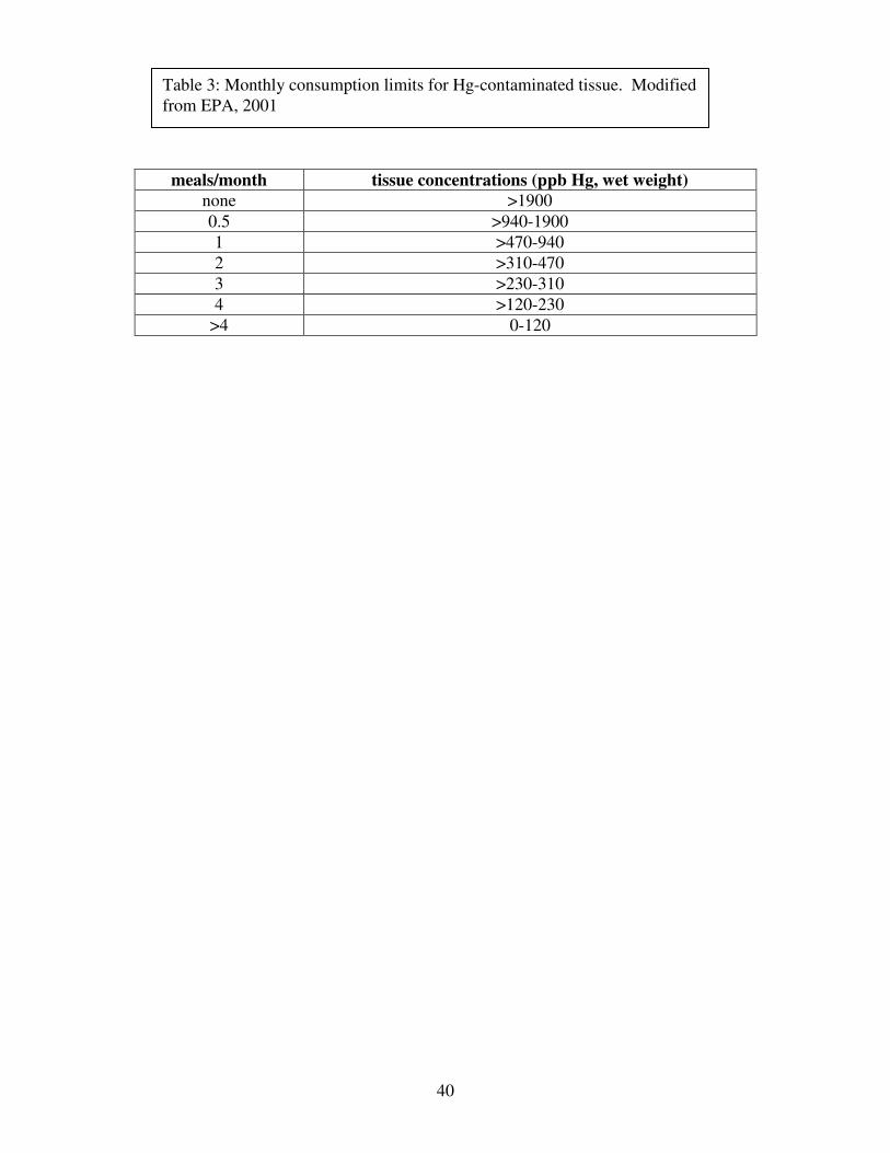
kg) (EPA, 2001). Table 3 lists the range of Hg concentrations associated with each consumption
31
limit category. These limits are based on Hg concentrations measured in fresh tissue. Since all
samples in this study were lyophilized, Hg concentrations have been reported on a dry weight
basis. In order to compare these Hg concentrations to the EPA’s risk-based consumption limits,
they have been converted to wet weights based on the average moisture content for each tissue
type (liver: 76%, kidney: 82%, leg muscle: 78%, and pectoral muscle: 81%). The above
equations can be modified to determine consumption limits for a specific consumer body mass
and meal size, but we have used the standard values here for simplicity. Table 3.1 lists these
consumption limits with their associated ranges of tissue Hg concentrations.
Statistical Analysis
Data were entered into Excel spreadsheets and analyzed using SAS v.8.1 software (SAS
Institute, Cary, NC). The number of turtles from an individual species varied from 2 to 8, with
most species represented by 4 to 6 specimens. Data for individual species were generally non-
normal by a Shapiro-Wilk test. Plots of Hg values showed that data were often highly skewed,
and there were many outliers. Variance and range of data also varied considerably among
species, and no single transformation was adequate to normalize the data and homogenize the
variances. Data were analyzed using both parametric (ANOVA, Pearson’s correlations) and
nonparametric methods (Kruskal-Wallis tests, Spearman’s correlations). Because the
assumptions of parametric statistics could not always be met, non-parametric methods were
primarily used. Both types of analyses generally led to the same conclusions regarding
relationships among variables and differences among tissues and species, suggesting that unmet
assumptions about normality and homogeneity of variance were not important factors
influencing the parametric analyses.
32
Chinemys reevesi Cuora amboinensis a b
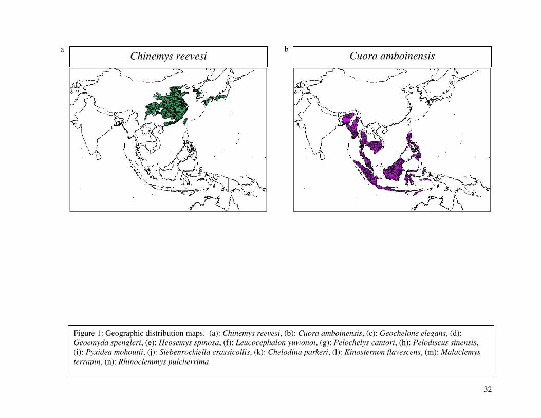
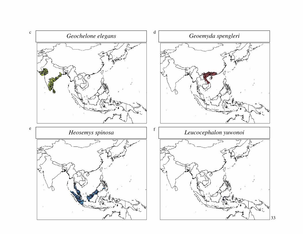
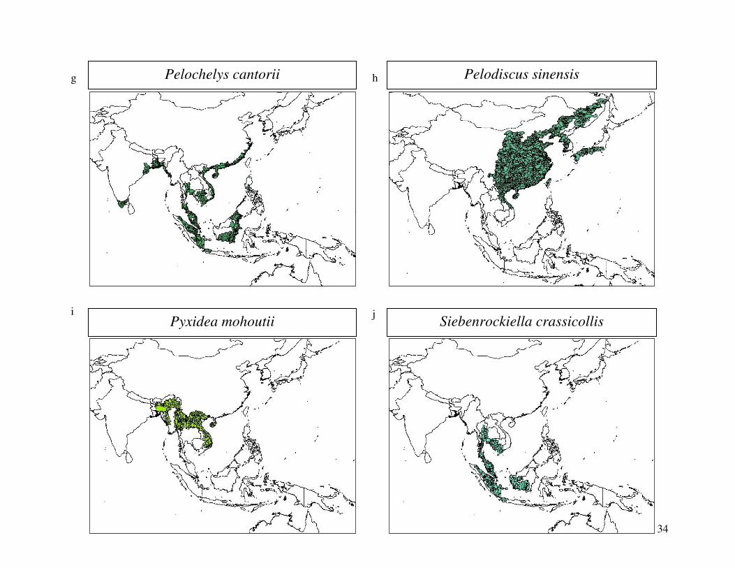
Figure 1: Geographic distribution maps. (a): Chinemys reevesi, (b): Cuora amboinensis, (c): Geochelone elegans, (d): Geoemyda spengleri, (e): Heosemys spinosa, (f): Leucocephalon yuwonoi, (g): Pelochelys cantori, (h): Pelodiscus sinensis, (i): Pyxidea mohoutii, (j): Siebenrockiella crassicollis, (k): Chelodina parkeri, (l): Kinosternon flavescens, (m): Malaclemys
terrapin, (n): Rhinoclemmys pulcherrima
33
Geochelone elegans c
Geoemyda spengleri d
Heosemys spinosa e
Leucocephalon yuwonoi f
34
Pelochelys cantorii g Pelodiscus sinensis h
Pyxidea mohoutii i
Siebenrockiella crassicollis j
35
Chelodina parkeri k
Kinosternon flavescens l
Malaclemys terrapin m
Rhinoclemmys pulcherrima n
36
Species Code
Species Name Common Name Geographic Range
Habitat Diet IUCN Status
CHRE Chinemys reevesi Reeve's turtle
Central/Eastern China (native), Japan and Korea (introduced)
large, slow-moving rivers
invertebrates, algae, aquatic plants
endangered
CUAM Cuora amboinensis Malayan box turtle
Bangladesh, India, Cambodia, Malaysia, Indonesia, Philippines, Thailand, Myanmar
swamps, rice paddies, small bodies of slow or stagnant water
aquatic plants, mollusks, small crustaceans, mushrooms, earthworms, plants
endangered
GEEL Geochelone elegans Indian star tortoise India, Pakistan, Sri Lanka
arid areas with abundant plants, prairies
fruits, vegetables, dead leaves, spiny vegetation
least concern
GESP Geoemyda spengleri Black-breasted leaf turtle Hainan Island, southern China, Vietnam
wooded, mountainous areas near wetlands and creeks
insects, earthworms, small invertebrates, fruit
endangered
Table 2: Life history characteristics of study species. The four-letter species code is created by combining the first two letters of the genus name with the first two letters of the species name.
37
HESP Heosemys spinosa Spiny turtle
southern Myanmar, Thailand, peninsular Malaysia, Indonesia, Singapore, Philippines
humid, montane forests
plants, vegetative debris, fallen fruit, insects, earthworms, carrion
endangered
LEYU Leucocephalon yuwonoi Sulawesi forest turtle Sulawesi (Indonesia)
semiaquatic; rocky, heavily vegetated areas near swamps and streams
fruits and leaves
critically endangered
PECA Pelochelys cantorii Cantor's giant softshell turtle
southern India, Bangladesh, Thailand, Myanmar, Cambodia, Vietnam, Laos, China, Borneo, eastern Sumatra, northern Java, Luzon (Phillipines)
estuaries, river deltas, freshwater streams, deep, slow-moving rivers
fish, crustaceans, mollusks,
endangered
PESI Pelodiscus sinensis Chinese softshell turtle
Eastern and central China, Taiwan (native), Japan, Thailand, Hawaii (introduced)
slow-moving rivers, canals, lakes, swamps, rice paddies
fish, crustaceans, mollusks, insects, worms, various larvae, leaves, seeds
vulnerable
38
PYMO Pyxidea mouhotii Keeled box turtle
Hainan Island, China, Vietnam, Thailand, Myanmar, India, Bangladesh, peninsular Malaysia, Laos, Cambodia
humid forested areas, foothills, rocky slopes
earthworms, mollusks, snails, fruit
endangered
SICR Siebenrockiella crassicollis Black mud turtle
Thailand, Vietnam, Java, Sumatra, Borneo, peninsular Malayasia, Myanmar, Singapore
marshes, ponds, slow-moving rivers, shallow warm waters
fruits, leaves, shrimp, amphibians, mollusks, fish
endangered
CHPA Chelodina parkeri Parker's snake-necked turtle
southern Papua New Guinea near Irian Jaya border
large lakes and rivers, temporary wetlands, estaries
fish, shrimp vulnerable
KIFL Kinosternon flavescens Yellow mud turtle
Central and southwestern United States, northern Mexico
slow-moving rivers, swamps, and marshes
insects, crustaceans, mollusks, amphibian, carrion, aquatic inverts
least concern
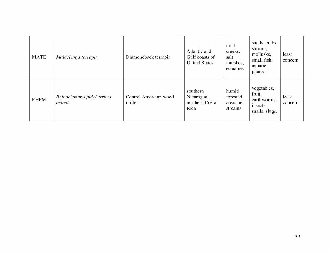
39
MATE Malaclemys terrapin Diamondback terrapin Atlantic and Gulf coasts of United States
tidal creeks, salt marshes, estuaries
snails, crabs, shrimp, mollusks, small fish, aquatic plants
least concern
RHPM Rhinoclemmys pulcherrima
manni
Central Amercian wood turtle
southern Nicaragua, northern Costa Rica
humid forested areas near streams
vegetables, fruit, earthworms, insects, snails, slugs.
least concern
40
meals/month tissue concentrations (ppb Hg, wet weight)
none >1900
0.5 >940-1900
1 >470-940
2 >310-470
3 >230-310
4 >120-230
>4 0-120
Table 3: Monthly consumption limits for Hg-contaminated tissue. Modified from EPA, 2001
41
RESULTS
Mercury
Tissue distribution:
Figure 2 shows the pattern of tissue Hg distribution for each species. Tissue distribution
of Hg followed a general pattern in which liver Hg was the highest, followed by kidney and
scutes. Muscle and follicles were generally lowest in Hg. Exceptions to this general pattern
include K. flavescens, for which most scute samples were similar to or higher than liver samples
in Hg; and G. spengleri, for which scute Hg greatly exceeded liver Hg. Kidney samples varied
greatly in Hg concentration relative to other tissues. Chelodina reevesi and L. yuwonoi both had
greater amounts of Hg in follicles than in kidney samples. Malaclemys terrapin and C. reevesi
had scute Hg levels exceeding kidney Hg.
Differences in Hg among species:
Table 4 lists the maximum, minimum, average, and median Hg concentrations of each
tissue for each species. Mercury concentrations in most tissues differed significantly among
species. For kidney, a Kruskal-Wallis test indicated a marginally significant difference among
species, but ANOVA indicated no such difference. As stated previously, kidney was the most
variable tissue in terms of Hg content.
Four species (P. sinensis, L. yuwonoi, G. elegans, and R. pulcherrima manni) had the
lowest range of Hg concentrations in the study, with most tissues <1000 ppb Hg. One G.
elegans liver sample had 1912 ppb Hg and one R. pulcherrima manni liver had 21234 ppb Hg.
Five species (C. parkeri, C. amboinensis, G. spengleri, H. spinosa, and P. cantorii), had
relatively moderate Hg levels, with all tissues <5000 ppb. For the five remaining species (C.
42
reevesi, K. flavescens, M. terrapin, P. mohoutii, and S. crassicollis), most tissues were <5000
ppb as well, but some tissue samples exceeded this value.
Differences in Hg among tissues:
In most species, there were significant differences in Hg among tissue types. Exceptions
were C. reevesi and G. elegans, where the Kruskal-Wallis tests indicated significant differences
among tissues while ANOVA did not. No significant difference in Hg was found between
tissues for P. mouhotii, C. parkeri, or R. pulcherrima manni.
Correlations among tissue Hg concentrations:
For P. mouhotii, claw Hg was strongly correlated with Hg in pectoral muscle (n=6,
rs=0.94286, p=0.0048) and scutes (n=6, rs=0.94286, p=0.0048). Scute Hg was also correlated
with pectoral muscle Hg (n=6, rs=1, p<0.0001). In C. amboinensis, liver Hg and kidney Hg were
highly correlated (n=7, rs=0.89286, p=0.0068).
Range of Hg values:
Species differed greatly in the range of Hg tissue concentrations among individuals
(Figure 2). Three species, G. spengleri, G. elegans, and L. yuwonoi, displayed the lowest
amount of variation between individuals in all tissues. G. spengleri had low variability in all
tissue types except for scutes. Although the range in scute Hg for this species was large, the
minimum scute Hg concentration was 1073 ppb, by far the highest minimum scute Hg
concentration of any species analyzed in this study. In fact, this minimum value was greater than
the maximum scute Hg measurement of all but four species (C. reevesi, K. flavescens, H.
spinosa, and P. mohoutii). For some species, the large range of Hg values was due to one
individual with Hg concentrations that were substantially higher than in its conspecifics. G.
elegans specimens displayed low variability in Hg concentrations in all tissues except liver,
which was heavily influenced by a single specimen. One turtle had a liver Hg concentration of
43
1912 ppb, while the average liver Hg of this species was 134 ppb when this individual was
excluded. This was also true for L. yuwonoi, where one individual had much higher Hg in its
liver than others sampled from this species. For C. amboinensis, two individuals had
substantially higher Hg in all tissues (except scute and claw) than the other six turtles in this
species.
In the remaining species, ranges of Hg values were relatively large for most tissues
sampled. However, in four species (H. spinosa, K. flavescens, R. pulcherrima manni, and S.
crassicollis), there was relatively little variability in Hg concentrations in muscle tissue.
Relationship of Hg to body size:
S. crassicollis and M. terrapin were the only species for which tissue Hg was
significantly related to body size (mass or standard carapace length [SCL]). For S. crassicollis,
kidney Hg (n=6, rs= -0.81168, p=0.0499) and scute Hg (n=6, rs=0.81168, p=0.0499) were both
significantly correlated with SCL. Liver Hg (n=6, rs= -0.82857, p=0.0416) was significantly
negatively correlated with mass. For M. terrapin, leg muscle Hg (n=5, rs=0.9, p=0.0374) was
significantly correlated with mass.
Differences in tissue Hg among diet groups:
To examine the influence diet has on tissue Hg, species were divided into three groups:
herbivores (G. elegans, H. spinosa, and L. yuwonoi), omnivores (R. pulcherrima manni, S.
crassicollis, C. reevesi, C. amboinensis, G. spengleri, and P. mohoutii), and carnivores (M.
terrapin, K. flavescens, P. sinensis, P. cantorii, and C. parkeri). Figure 3 shows the median Hg
values of each tissue type for each diet group. Diet groups differed significantly in Hg for all
tissues except kidney and liver (claw: n=68, χ2=36.053, df=2, p<0.0001; follicle: n=30,
χ2=6.2418, df=2, p=0.0441, leg muscle: n=64, χ2=30.1427, df=2, p<0.0001, pectoral muscle:
n=59, χ2=26.8445, df=2, p<0.0001, scute: n=58, χ2=13.1058, df=2, p=0.0014). As shown in
44
figure 3, the general pattern of Hg in carnivores>Hg in omnivores>Hg in herbivores was
displayed in liver and kidney samples, even though diet groups did not differ significantly in Hg
for these two tissue types.
Differences in tissue Hg between sexes:
We tested for differences between sexes by pooling all tissues within each species. P.
mouhotii was the only species for which tissue Hg differed between sexes; males had
significantly less Hg than females (n=35, χ2=7.5044, p=0.0062).
Stable Isotopes
There was no significant correlation between δ15N values and Hg when all species were
pooled. There was, however, a strong positive correlation between δ13C and δ15N values for
each tissue type when all species were pooled (claw: n=57, rs=0.76763, p<0.0001; follicle: n=27,
rs=0.6854, p<0.0001; kidney: n=38, 0.72404, p<0.0001; leg muscle: n=60, rs=0.70036,
p<0.0001; liver: n=56, rs=0.75783, p<0.0001; pectoral muscle: n=54, rs=0.82159, p<0.0001;
scute: n=55, rs=0.58624, p<0.0001). This relationship is displayed in Figure 4. There was also a
strong positive correlation between δ15N and δ13C values for four species when all tissues were
pooled (C. reevesi: n=22, rs=0.69735, p=0.0003; H. spinosa: n=40, rs=0.75474, p<0.0001; L.
yuwonoi: n=37, rs=0.76268, p<0.0001; M. terrapin: n=24, rs=0.6687, p=0.0004). This
relationship is displayed in Figure 5.
For each species, δ13C and δ
15N values were plotted by tissue type (liver, kidney, pectoral
muscle, leg muscle, claw, scute, and follicle) for each individual in figures 6 and 7, respectively.
Species differed greatly in both the variance in δ13C and δ15N values among individuals of a
species and the variance in values among tissues in an individual. Some species, such as G.
spengleri, had relatively small ranges of δ13C and δ15N values among individuals, while others,
such as S. crassicollis, had larger ranges. For some species, such as C. amboinenis, δ13C and
45
δ15N values differed little between tissue types. Other species, such as P. sinensis, had larger
differences in δ13C and δ15N values between tissues.
Figures 8 and 9 show the ranges of δ13C and δ15N values, respectively, measured in liver
samples of each species. Values for liver samples were used because, due to its high metabolic
rate, the stable isotope composition of the liver closely resembles that of the diet (Tieszen et al.,
1983). Species are grouped into categories based on habitat type in Figure 8. Stable carbon
isotope values for aquatic species ranged from -17 to -30‰, while values for terrestrial species
defined a slightly smaller range, from -21 to -27‰. In Figure 9, species are grouped into
categories based on habitat and diet. Stable nitrogen isotope values ranged from 8 to 12‰ for
aquatic carnivores, 7.7-10.3‰ for terrestrial omnivores, 5.6-10.3‰ for aquatic omnivores, and
6.5-9.5‰ for terrestrial herbivores.
Comparison of Hg Levels to Risk-Based Consumption Limits
All edible samples (liver, kidney, and muscle) were divided into seven categories based
on the CRmm: do not eat, 0.5 meals/month, 1 meal/month, 2 meals/month, 3 meals/month, 4
meals/month, and >4 meals/month. Figure 10 shows the proportion of samples in each
consumption category for each tissue type.
Of all edible tissues, Hg was highest in liver for all species, followed by kidney and
muscle. Nine of 62 (14%) liver samples analyzed exceeded the 1900 ppb consumption threshold
recommended for all adults, including those of C. reevesi, S. crassicollis, M. terrapin, H.
spinosa, and P. mohoutii. Twenty-one of 62 (34%) liver samples had Hg levels within or above
the 470-940 ppb range recommended for one meal per month. The highest Hg concentrations
measured in this study were in livers from a single H. spinosa specimen (4,768 ppb), a R.
pulcherrima manni specimen (5,017 ppb), and two C. reevesi specimens (7,443 ppb and 16,561
ppb).
46
Nine of 42 (10%) kidney samples had levels of Hg above the range recommended for one
meal per month. These were samples collected from an individual H. spinosa, a C. parkeri
specimen, and two P. mohoutii individuals. One hundred nineteen of 125 (95%) muscle samples
had Hg concentrations below the level recommended for four meals per month. Only 6 of 125
(5%) of muscle samples contained enough Hg to require consumption limitations, including
muscles from C. parkeri, C. reevesi, P. cantorii, and P. mohoutii.
Figure 11 shows the proportion of samples in each consumption category for each
species. For many species that are popular in the food trade, a considerable proportion of edible
samples were within ranges recommended for limited consumption. Three of 18 (17%) M.
terrapin samples had Hg levels within or above the range recommended for no more than one
meal per month, and one liver sample was above the 1900 ppb consumption threshold. Four of
14 (28%) C. reevesi samples were within or above the range of Hg concentrations recommended
for no more than one meal per month, and two liver samples were above the 1900 ppb
consumption threshold. Three of 19 (15%) of S. crassicollis samples had Hg levels within or
above the range recommended for no more than one meal every two months, and two liver
samples were above the 1900 ppb consumption threshold. Two of eight (25%) of P. cantorii
samples were within the range of Hg concentrations recommended for no more than one meal
every two months. Three of seven (43%) of C. parkeri samples had Hg levels within or above
the range recommended for no more than one meal per month.
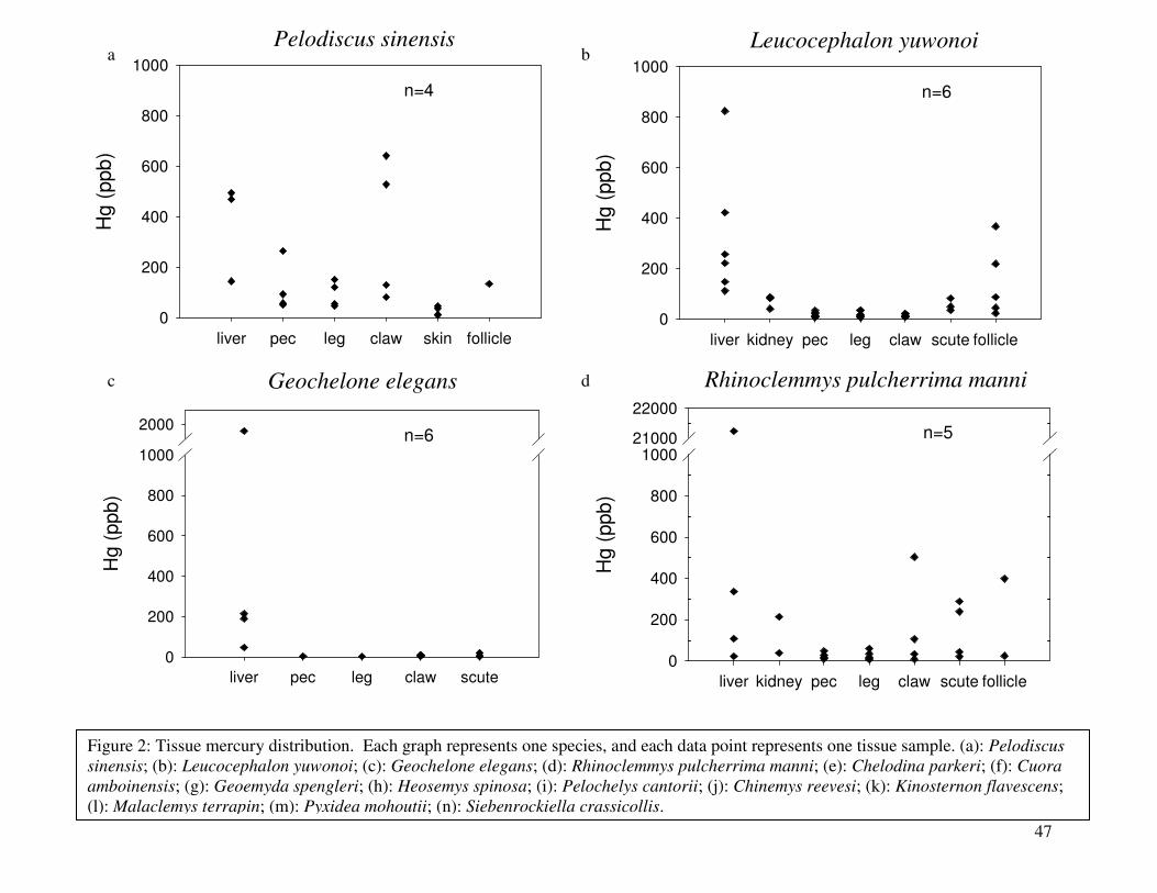
47
GEEL
liver pec leg claw scute
Hg (
ppb)
0
200
400
600
800
1000
2000
LEYU
liver kidney pec leg claw scute follicle
Hg
(ppb
)
0
200
400
600
800
1000
PESI
liver pec leg claw skin follicle
Hg
(ppb
)
0
200
400
600
800
1000
RHPM
liver kidney pec leg claw scute follicle
Hg
(ppb
)
0
200
400
600
800
100021000
22000
a
c
Figure 2: Tissue mercury distribution. Each graph represents one species, and each data point represents one tissue sample. (a): Pelodiscus
sinensis; (b): Leucocephalon yuwonoi; (c): Geochelone elegans; (d): Rhinoclemmys pulcherrima manni; (e): Chelodina parkeri; (f): Cuora
amboinensis; (g): Geoemyda spengleri; (h): Heosemys spinosa; (i): Pelochelys cantorii; (j): Chinemys reevesi; (k): Kinosternon flavescens; (l): Malaclemys terrapin; (m): Pyxidea mohoutii; (n): Siebenrockiella crassicollis.
b
d
Pelodiscus sinensis Leucocephalon yuwonoi
Geochelone elegans Rhinoclemmys pulcherrima manni
n=6 n=5
n=4 n=6
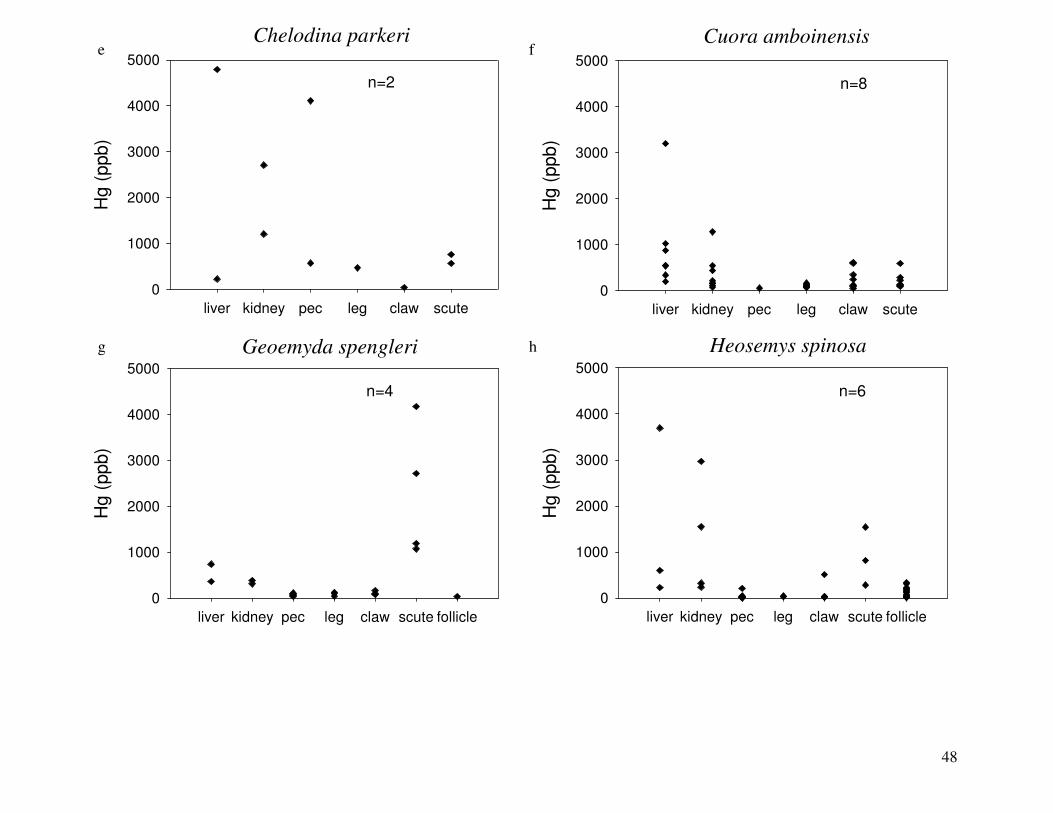
48
48
CHPA
liver kidney pec leg claw scute
Hg
(ppb)
0
1000
2000
3000
4000
5000
CUAM
liver kidney pec leg claw scute
Hg
(ppb
)
0
1000
2000
3000
4000
5000
GESP
liver kidney pec leg claw scute follicle
Hg
(ppb)
0
1000
2000
3000
4000
5000
HESP
liver kidney pec leg claw scute follicle
Hg
(ppb
)
0
1000
2000
3000
4000
5000
e
g
Cuora amboinensis f
h
Chelodina parkeri
Geoemyda spengleri Heosemys spinosa
n=4
n=8
n=6
n=2
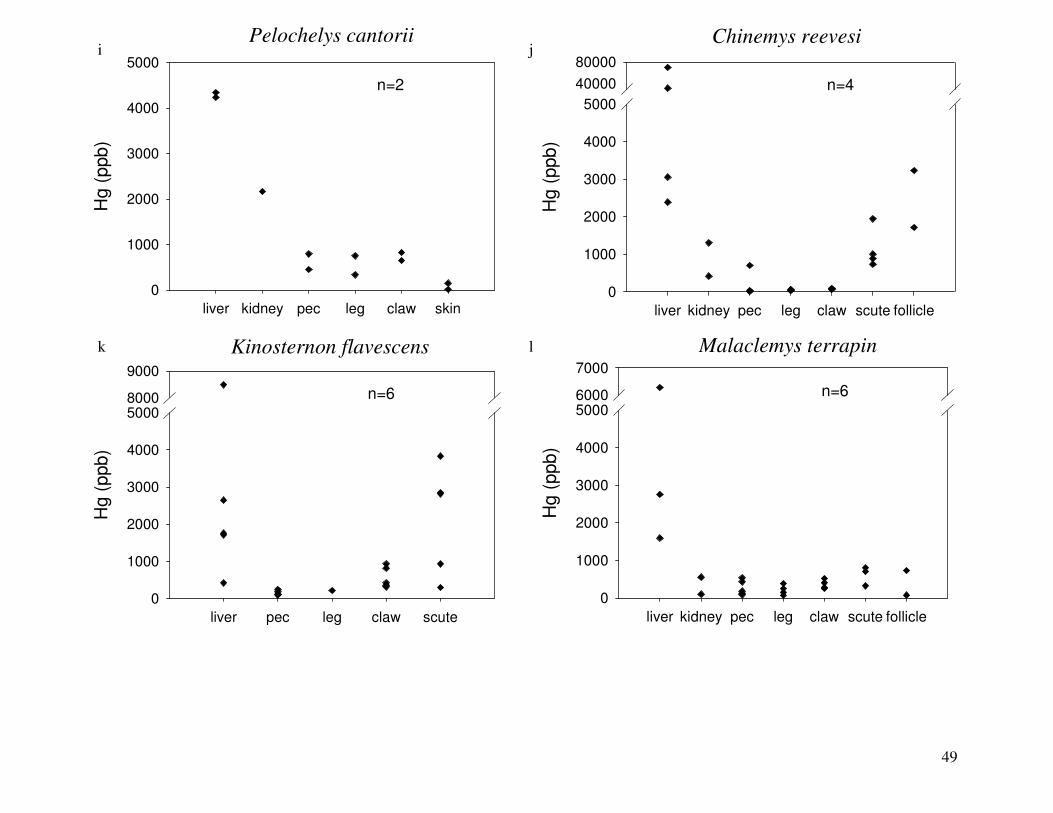
49
49
PECA
liver kidney pec leg claw skin
Hg
(p
pb
)
0
1000
2000
3000
4000
5000
CHRE
liver kidney pec leg claw scute follicle
Hg
(ppb
)
0
1000
2000
3000
4000
5000
40000
80000
KIFL
liver pec leg claw scute
Hg
(p
pb
)
0
1000
2000
3000
4000
50008000
9000
MATE
liver kidney pec leg claw scute follicle
Hg
(ppb
)
0
1000
2000
3000
4000
50006000
7000
i
k
j
l
Pelochelys cantorii Chinemys reevesi
Kinosternon flavescens Malaclemys terrapin
n=6
n=4
n=6
n=2
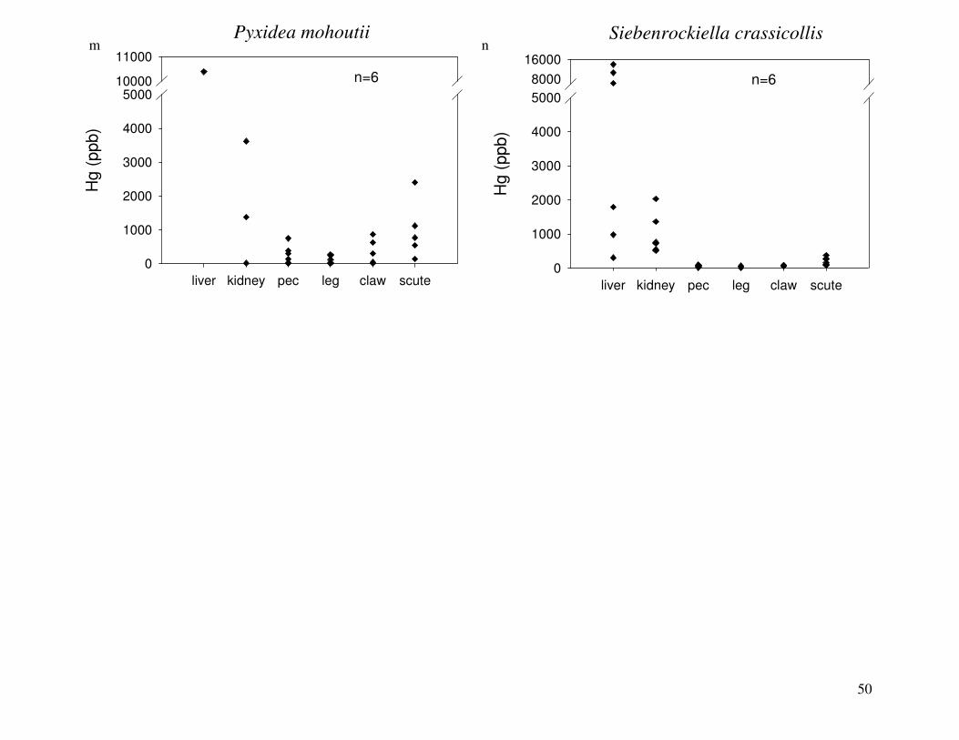
50
PYMO
liver kidney pec leg claw scute
Hg
(p
pb)
0
1000
2000
3000
4000
500010000
11000
SICR
liver kidney pec leg claw scute
Hg (
ppb)
0
1000
2000
3000
4000
5000
8000
16000m
n Pyxidea mohoutii Siebenrockiella crassicollis
n=6 n=6
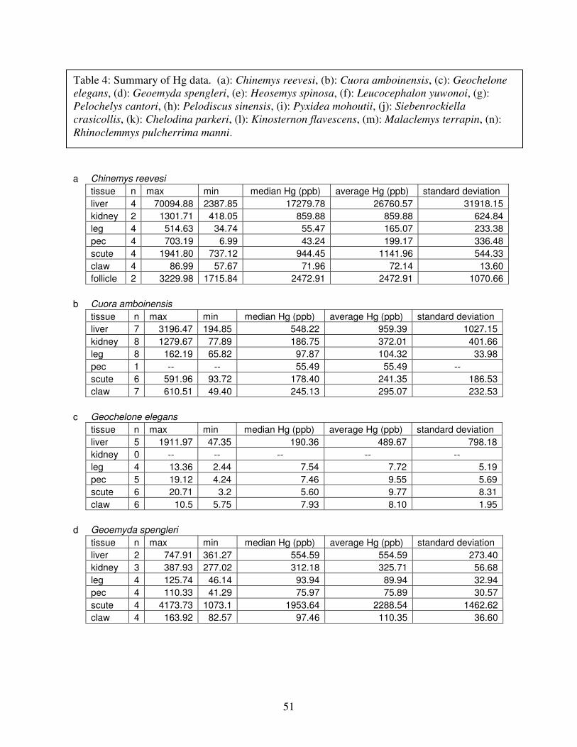
51
a Chinemys reevesi
tissue n max min median Hg (ppb) average Hg (ppb) standard deviation
liver 4 70094.88 2387.85 17279.78 26760.57 31918.15
kidney 2 1301.71 418.05 859.88 859.88 624.84
leg 4 514.63 34.74 55.47 165.07 233.38
pec 4 703.19 6.99 43.24 199.17 336.48
scute 4 1941.80 737.12 944.45 1141.96 544.33
claw 4 86.99 57.67 71.96 72.14 13.60
follicle 2 3229.98 1715.84 2472.91 2472.91 1070.66
b Cuora amboinensis
tissue n max min median Hg (ppb) average Hg (ppb) standard deviation
liver 7 3196.47 194.85 548.22 959.39 1027.15
kidney 8 1279.67 77.89 186.75 372.01 401.66
leg 8 162.19 65.82 97.87 104.32 33.98
pec 1 -- -- 55.49 55.49 --
scute 6 591.96 93.72 178.40 241.35 186.53
claw 7 610.51 49.40 245.13 295.07 232.53
c Geochelone elegans
tissue n max min median Hg (ppb) average Hg (ppb) standard deviation
liver 5 1911.97 47.35 190.36 489.67 798.18
kidney 0 -- -- -- -- --
leg 4 13.36 2.44 7.54 7.72 5.19
pec 5 19.12 4.24 7.46 9.55 5.69
scute 6 20.71 3.2 5.60 9.77 8.31
claw 6 10.5 5.75 7.93 8.10 1.95
d Geoemyda spengleri
tissue n max min median Hg (ppb) average Hg (ppb) standard deviation
liver 2 747.91 361.27 554.59 554.59 273.40
kidney 3 387.93 277.02 312.18 325.71 56.68
leg 4 125.74 46.14 93.94 89.94 32.94
pec 4 110.33 41.29 75.97 75.89 30.57
scute 4 4173.73 1073.1 1953.64 2288.54 1462.62
claw 4 163.92 82.57 97.46 110.35 36.60
Table 4: Summary of Hg data. (a): Chinemys reevesi, (b): Cuora amboinensis, (c): Geochelone
elegans, (d): Geoemyda spengleri, (e): Heosemys spinosa, (f): Leucocephalon yuwonoi, (g): Pelochelys cantori, (h): Pelodiscus sinensis, (i): Pyxidea mohoutii, (j): Siebenrockiella
crasicollis, (k): Chelodina parkeri, (l): Kinosternon flavescens, (m): Malaclemys terrapin, (n): Rhinoclemmys pulcherrima manni.
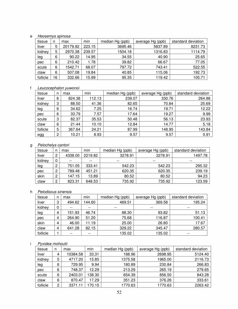
52
e Heosemys spinosa
tissue n max min median Hg (ppb) average Hg (ppb) standard deviation
liver 5 20179.92 223.15 3695.46 5837.89 8231.73
kidney 5 2970.38 239.57 1504.18 1316.83 1114.79
leg 6 90.22 14.95 34.55 40.90 25.65
pec 6 210.42 1.78 39.82 66.67 77.05
scute 6 1542.71 68.07 797.72 743.41 522.55
claw 6 507.08 19.84 40.85 115.06 192.73
follicle 16 332.66 15.99 95.35 119.42 105.71
f Leucocephalon yuwonoi
tissue n max min median Hg (ppb) average Hg (ppb) standard deviation
liver 6 824.38 112.13 239.07 330.76 264.88
kidney 3 88.50 41.36 82.65 70.84 25.69
leg 6 34.62 7.25 16.74 19.71 12.22
pec 6 33.79 7.57 17.64 19.27 9.99
scute 3 82.37 35.53 50.48 56.13 23.93
claw 6 21.44 10.10 12.84 14.77 5.18
follicle 5 367.64 24.21 87.99 148.95 143.84
egg 2 10.21 8.93 9.57 9.57 0.91
g Pelochelys cantori
tissue n max min median Hg (ppb) average Hg (ppb) standard deviation
liver 2 4338.00 2219.82 3278.91 3278.91 1497.78
kidney 0 -- -- -- -- --
leg 2 751.05 333.41 542.23 542.23 295.32
pec 2 789.48 451.21 620.35 620.35 239.19
skin 2 147.15 13.89 80.52 80.52 94.23
claw 2 823.31 648.53 735.92 735.92 123.59
h Pelodiscus sinensis
tissue n max min median Hg (ppb) average Hg (ppb) standard deviation
liver 3 494.62 144.60 469.51 369.58 195.24
kidney 0 -- -- -- -- --
leg 4 151.93 46.74 88.30 93.82 51.13
pec 4 264.90 51.20 75.68 116.87 100.41
skin 4 46.00 11.19 25.00 26.80 17.67
claw 4 641.28 82.15 329.22 345.47 280.57
follicle 1 -- -- 135.02 135.02 --
i Pyxidea mohoutii
tissue n max min median Hg (ppb) average Hg (ppb) standard deviation
liver 4 10384.58 33.31 188.96 2698.95 5124.40
kidney 5 4717.20 15.85 1375.58 1965.00 2116.73
leg 6 729.95 9.94 180.89 230.84 266.83
pec 6 748.37 12.29 213.29 265.19 279.65
scute 6 2403.01 138.30 654.39 856.50 843.28
claw 6 870.47 17.29 351.23 376.26 333.61
follicle 2 3371.11 170.15 1770.63 1770.63 2263.42
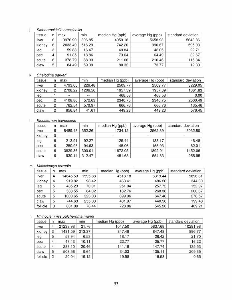
53
j Siebenrockiella crassicollis
tissue n max min median Hg (ppb) average Hg (ppb) standard deviation
liver 6 13976.90 306.85 4059.18 5658.93 5643.86
kidney 6 2033.49 516.29 742.20 990.67 595.03
leg 3 59.83 16.47 49.84 42.05 22.71
pec 4 91.85 18.86 73.64 64.49 32.67
scute 6 378.79 88.03 211.66 210.46 115.34
claw 5 84.49 59.39 80.32 73.77 12.83
k Chelodina parkeri
tissue n max min median Hg (ppb) average Hg (ppb) standard deviation
liver 2 4793.05 226.48 2509.77 2509.77 3229.05
kidney 2 2708.22 1206.56 1957.39 1957.39 1061.83
leg 1 -- -- 468.58 468.58 0.00
pec 2 4108.86 572.63 2340.75 2340.75 2500.49
scute 2 762.54 570.97 666.76 666.76 135.46
claw 2 856.84 41.61 449.23 449.23 576.45
l Kinosternon flavescens
tissue n max min median Hg (ppb) average Hg (ppb) standard deviation
liver 6 8489.48 352.26 1734.12 2562.39 3032.80
kidney 0 -- -- -- -- --
leg 6 213.91 92.27 125.44 138.17 46.48
pec 6 250.95 94.63 145.06 155.93 62.01
scute 6 3829.36 300.01 1872.05 1892.91 1452.06
claw 6 930.14 312.47 451.63 554.83 255.95
m Malaclemys terrapin
tissue n max min median Hg (ppb) average Hg (ppb) standard deviation
liver 4 14645.53 1595.88 4518.18 6319.44 5896.81
kidney 4 919.82 98.42 463.41 486.26 344.30
leg 5 435.23 70.01 251.04 257.72 152.97
pec 5 533.55 84.02 182.76 268.36 200.87
scute 5 1000.65 323.03 699.96 647.46 278.57
claw 5 744.63 255.03 401.97 440.56 199.48
follicle 3 831.09 76.44 728.06 545.20 409.21
n Rhinoclemmys pulcherrima manni
tissue n max min median Hg (ppb) average Hg (ppb) standard deviation
liver 4 21233.98 21.76 1047.50 5837.68 10291.98
kidney 3 1481.59 213.37 847.48 847.48 896.77
leg 5 59.94 6.53 18.17 26.42 21.70
pec 4 47.43 10.11 22.77 25.77 16.22
scute 4 288.10 20.46 141.19 147.74 135.53
claw 5 503.56 9.64 34.03 135.11 209.35
follicle 2 20.04 19.12 19.58 19.58 0.65
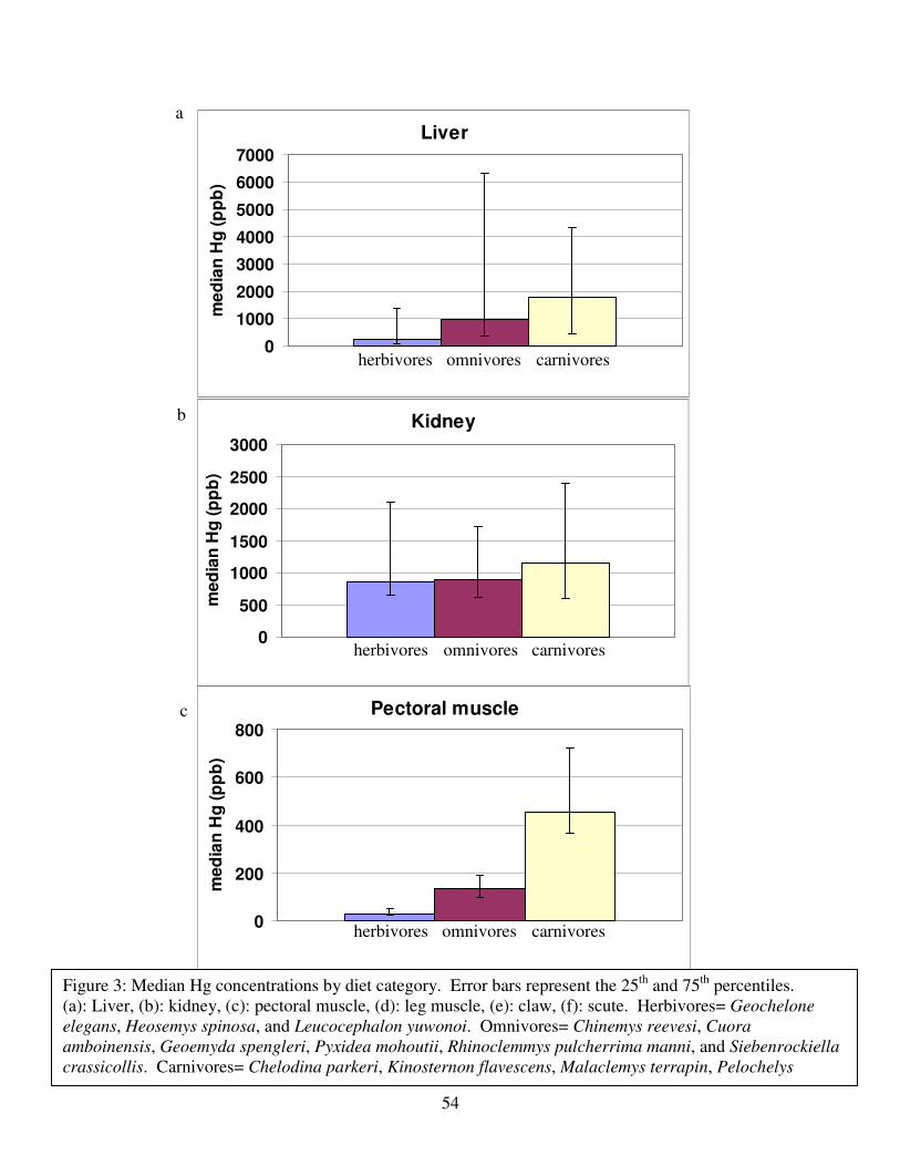
54
Pectoral muscle
0
200
400
600
800
med
ian
Hg
(p
pb
)
Kidney
0
500
1000
1500
2000
2500
3000
med
ian
Hg
(p
pb
)
Liver
0
1000
2000
3000
4000
5000
6000
7000
me
dia
n H
g (p
pb
)
herbivores
herbivores
herbivores
omnivores
omnivores
omnivores
carnivores
carnivores
carnivores
Figure 3: Median Hg concentrations by diet category. Error bars represent the 25th and 75th percentiles. (a): Liver, (b): kidney, (c): pectoral muscle, (d): leg muscle, (e): claw, (f): scute. Herbivores= Geochelone
elegans, Heosemys spinosa, and Leucocephalon yuwonoi. Omnivores= Chinemys reevesi, Cuora
amboinensis, Geoemyda spengleri, Pyxidea mohoutii, Rhinoclemmys pulcherrima manni, and Siebenrockiella
crassicollis. Carnivores= Chelodina parkeri, Kinosternon flavescens, Malaclemys terrapin, Pelochelys
cantorii, and Pelodiscus sinensis.
a
b
c
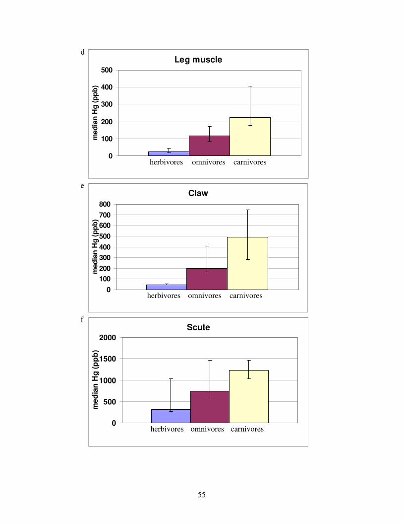
55
Scute
0
500
1000
1500
2000
med
ian
Hg
(p
pb
)
Claw
0
100
200
300
400
500
600
700
800
med
ian
Hg
(p
pb
)
Leg muscle
0
100
200
300
400
500
med
ian
Hg
(p
pb
)
herbivores
herbivores
herbivores
omnivores
omnivores
omnivores
carnivores
carnivores
carnivores
d
e
f
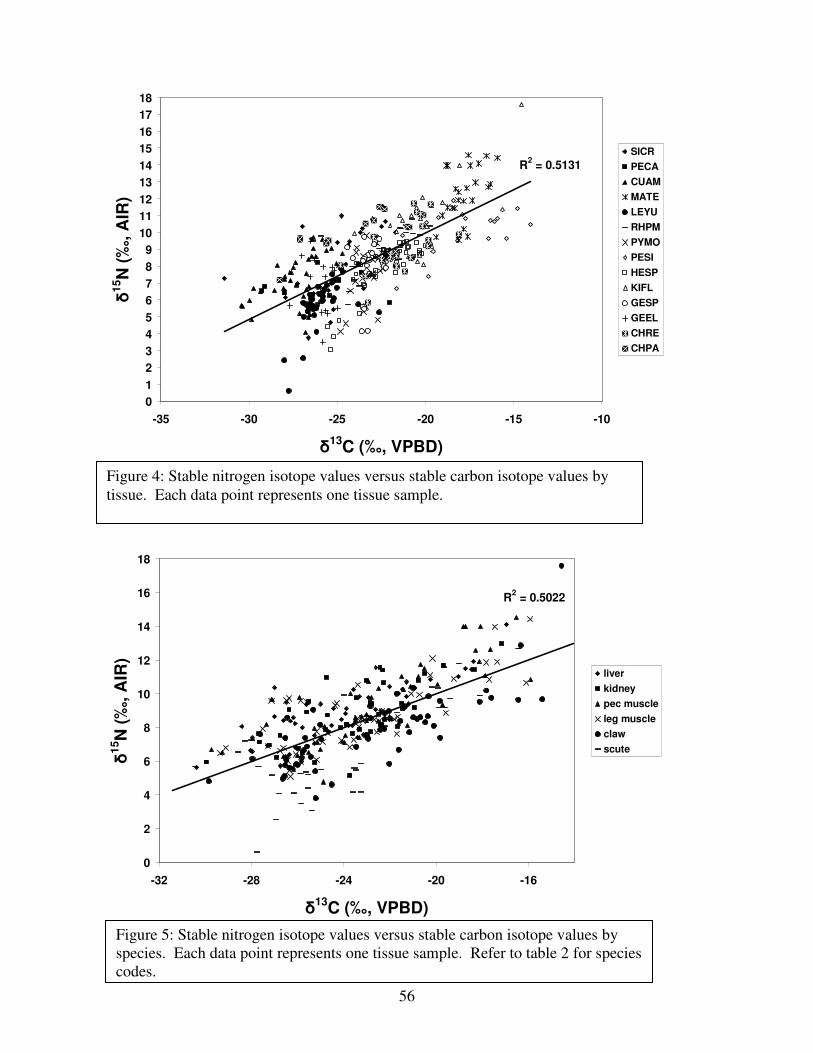
56
R2 = 0.5131
0
1
2
3
4
5
6
7
8
9
10
11
12
13
14
15
16
17
18
-35 -30 -25 -20 -15 -10
δ13
C (‰, VPBD)
δ1
5N
(‰
, A
IR)
SICR
PECA
CUAM
MATE
LEYU
RHPM
PYMO
PESI
HESP
KIFL
GESP
GEEL
CHRE
CHPA
R2 = 0.5022
0
2
4
6
8
10
12
14
16
18
-32 -28 -24 -20 -16
δ13
C (‰, VPBD)
δ1
5N
(‰
, A
IR)
liver
kidney
pec muscle
leg muscle
claw
scute
Figure 4: Stable nitrogen isotope values versus stable carbon isotope values by tissue. Each data point represents one tissue sample.
Figure 5: Stable nitrogen isotope values versus stable carbon isotope values by species. Each data point represents one tissue sample. Refer to table 2 for species codes.
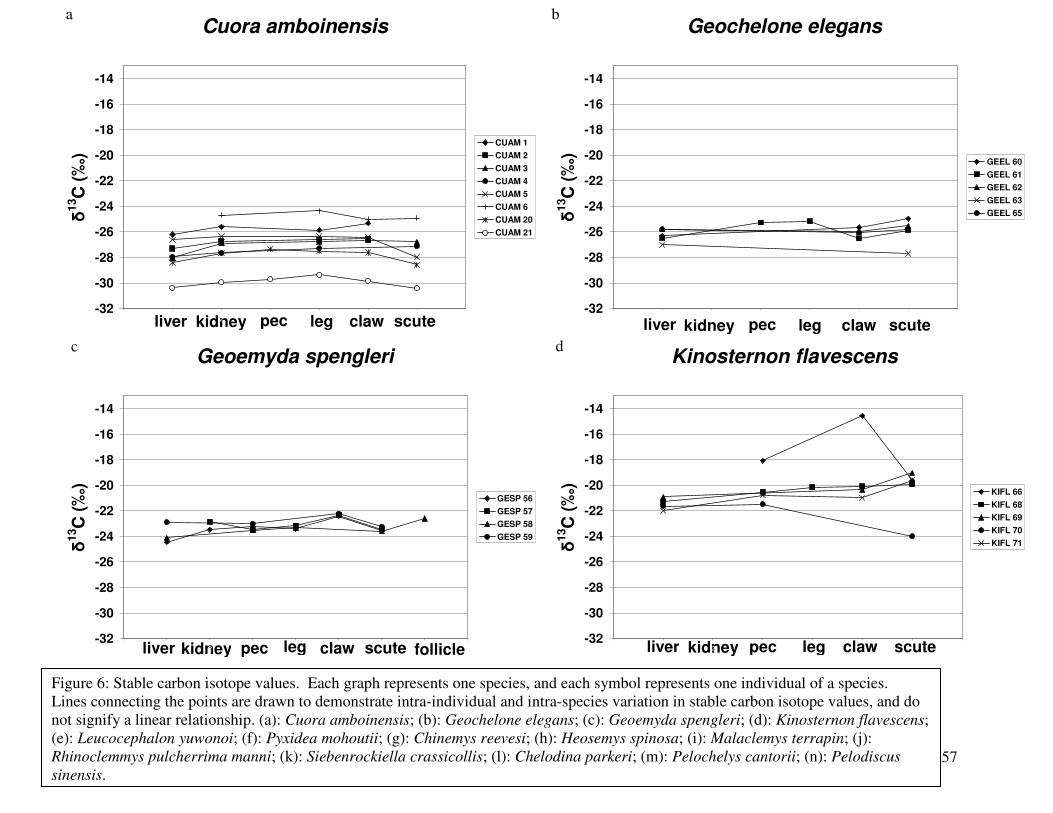
57
kidney
kidney
a
c
kidney
kidney
Cuora amboinensis
-32
-30
-28
-26
-24
-22
-20
-18
-16
-14
0 1 2 3 4 5 6 7
δ13C
(‰
)
CUAM 1
CUAM 2
CUAM 3
CUAM 4
CUAM 5
CUAM 6
CUAM 20
CUAM 21
Geochelone elegans
-32
-30
-28
-26
-24
-22
-20
-18
-16
-14
0 1 2 3 4 5 6 7
δ13C
(‰
)
GEEL 60
GEEL 61
GEEL 62
GEEL 63
GEEL 65
Geoemyda spengleri
-32
-30
-28
-26
-24
-22
-20
-18
-16
-14
0 1 2 3 4 5 6 7 8
δ13C
(‰
)
GESP 56
GESP 57
GESP 58
GESP 59
Kinosternon flavescens
-32
-30
-28
-26
-24
-22
-20
-18
-16
-14
0 1 2 3 4 5 6 7
δ13C
(‰
)
KIFL 66
KIFL 68
KIFL 69
KIFL 70
KIFL 71
liver pec leg claw scute follicle
Figure 6: Stable carbon isotope values. Each graph represents one species, and each symbol represents one individual of a species. Lines connecting the points are drawn to demonstrate intra-individual and intra-species variation in stable carbon isotope values, and do not signify a linear relationship. (a): Cuora amboinensis; (b): Geochelone elegans; (c): Geoemyda spengleri; (d): Kinosternon flavescens; (e): Leucocephalon yuwonoi; (f): Pyxidea mohoutii; (g): Chinemys reevesi; (h): Heosemys spinosa; (i): Malaclemys terrapin; (j): Rhinoclemmys pulcherrima manni; (k): Siebenrockiella crassicollis; (l): Chelodina parkeri; (m): Pelochelys cantorii; (n): Pelodiscus
sinensis.
liver pec leg claw scute
b
d
liver pec leg claw scute
liver pec leg claw scute
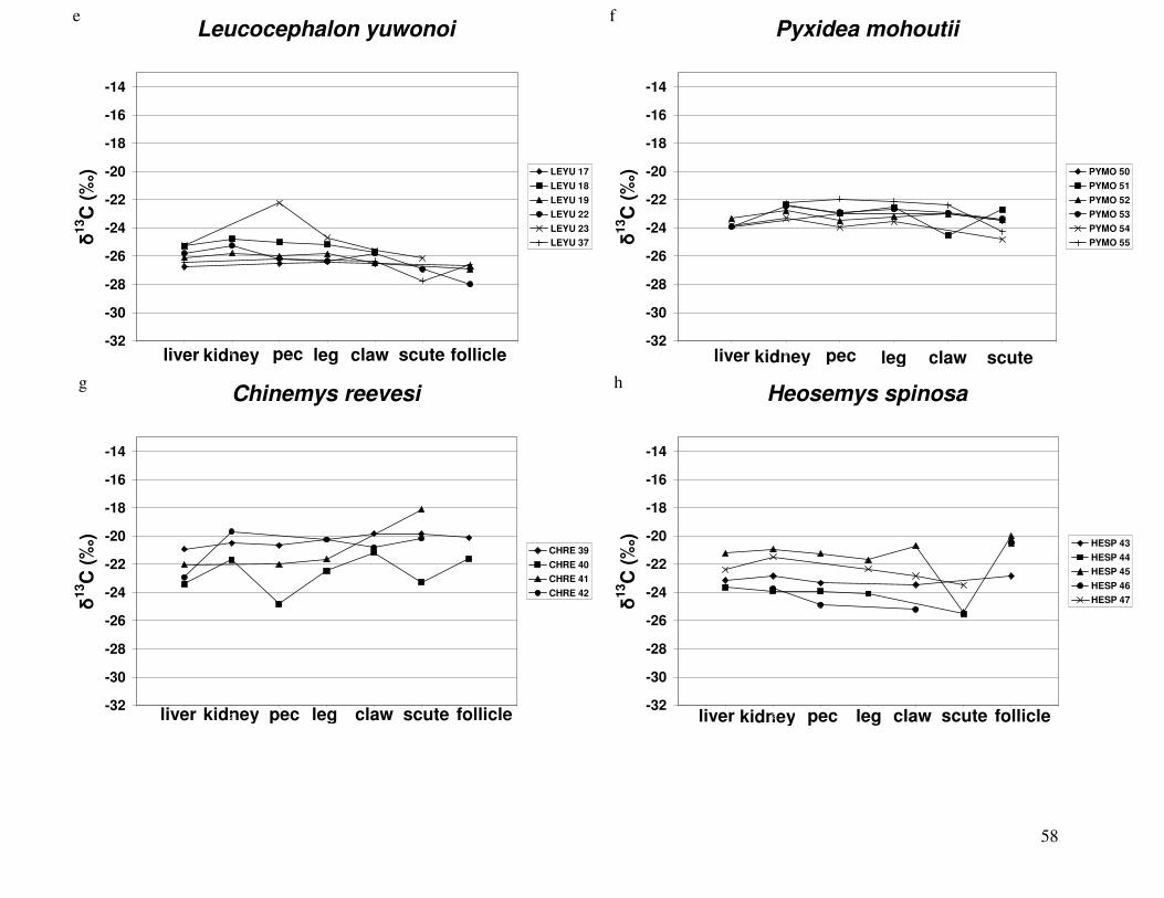
58
e
g
kidney kidney
kidney kidney
Leucocephalon yuwonoi
-32
-30
-28
-26
-24
-22
-20
-18
-16
-14
0 1 2 3 4 5 6 7 8
δ13C
(‰
) LEYU 17
LEYU 18
LEYU 19
LEYU 22
LEYU 23
LEYU 37
Pyxidea mohoutii
-32
-30
-28
-26
-24
-22
-20
-18
-16
-14
0 1 2 3 4 5 6 7
δ13C
(‰
) PYMO 50
PYMO 51
PYMO 52
PYMO 53
PYMO 54
PYMO 55
Chinemys reevesi
-32
-30
-28
-26
-24
-22
-20
-18
-16
-14
0 1 2 3 4 5 6 7 8
δ13C
(‰
)
CHRE 39
CHRE 40
CHRE 41
CHRE 42
Heosemys spinosa
-32
-30
-28
-26
-24
-22
-20
-18
-16
-14
0 1 2 3 4 5 6 7 8
δ13C
(‰
)
HESP 43
HESP 44
HESP 45
HESP 46
HESP 47
f
h
liver pec leg claw scute follicle liver pec leg claw scute
liver pec leg claw scute follicle liver pec leg claw scute follicle
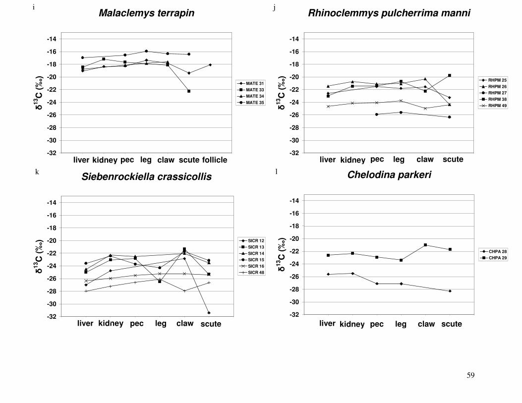
59
i
k
kidney kidney
kidney kidney
Malaclemys terrapin
-32
-30
-28
-26
-24
-22
-20
-18
-16
-14
0 1 2 3 4 5 6 7 8
δ13C
(‰
)
MATE 31
MATE 33
MATE 34
MATE 35
Rhinoclemmys pulcherrima manni
-32
-30
-28
-26
-24
-22
-20
-18
-16
-14
0 1 2 3 4 5 6 7
δ13C
(‰
)
RHPM 25
RHPM 26
RHPM 27
RHPM 38
RHPM 49
Siebenrockiella crassicollis
-32
-30
-28
-26
-24
-22
-20
-18
-16
-14
0 1 2 3 4 5 6 7
δ13C
(‰
) SICR 12
SICR 13
SICR 14
SICR 15
SICR 16
SICR 48
Chelodina parkeri
-32
-30
-28
-26
-24
-22
-20
-18
-16
-14
0 1 2 3 4 5 6 7
δ13C
(‰
)
CHPA 28
CHPA 29
j
l
liver pec leg claw scute follicle liver pec leg claw scute
liver pec leg claw scute liver pec leg claw scute
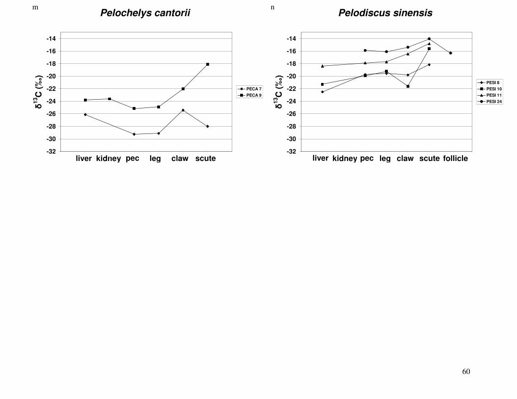
60
m
kidney kidney
Pelochelys cantorii
-32
-30
-28
-26
-24
-22
-20
-18
-16
-14
0 1 2 3 4 5 6 7
δ13C
(‰
)
PECA 7
PECA 9
Pelodiscus sinensis
-32
-30
-28
-26
-24
-22
-20
-18
-16
-14
0 1 2 3 4 5 6 7 8
δ13C
(‰
)
PESI 8
PESI 10
PESI 11
PESI 24
n
liver pec leg claw scute liver pec leg claw scute follicle
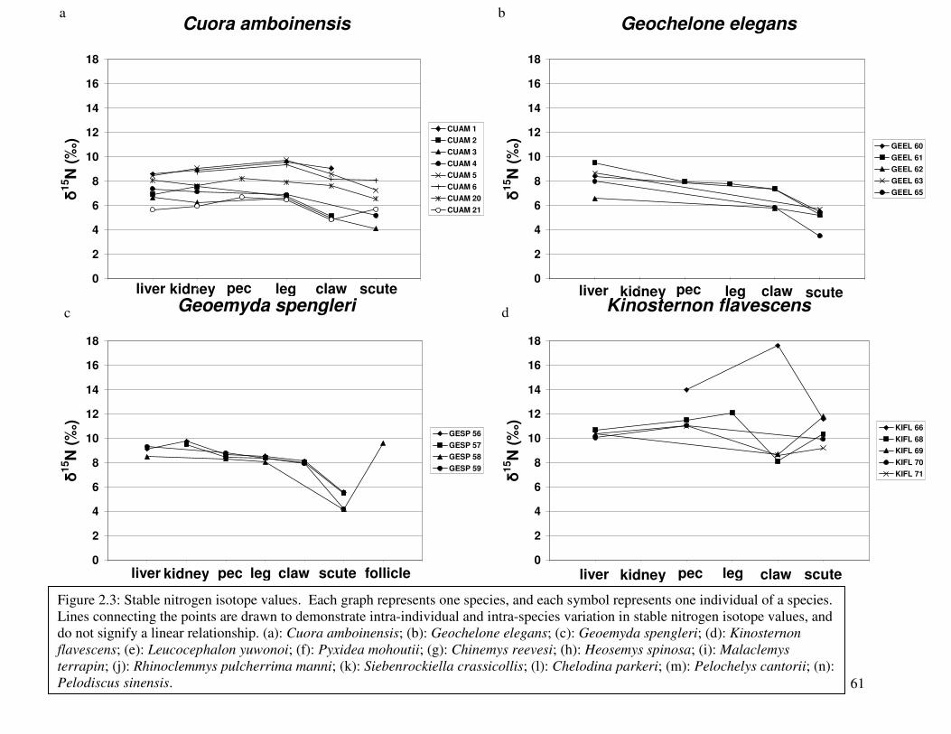
61
a
c
kidney kidney
kidney kidney
Cuora amboinensis
0
2
4
6
8
10
12
14
16
18
0 1 2 3 4 5 6 7
δ15N
(‰
)
CUAM 1
CUAM 2
CUAM 3
CUAM 4
CUAM 5
CUAM 6
CUAM 20
CUAM 21
Geochelone elegans
0
2
4
6
8
10
12
14
16
18
0 1 2 3 4 5 6 7
δ15N
(‰
)
GEEL 60
GEEL 61
GEEL 62
GEEL 63
GEEL 65
Geoemyda spengleri
0
2
4
6
8
10
12
14
16
18
0 1 2 3 4 5 6 7 8
δ15N
(‰
)
GESP 56
GESP 57
GESP 58
GESP 59
Kinosternon flavescens
0
2
4
6
8
10
12
14
16
18
0 1 2 3 4 5 6 7
δ15N
(‰
)
KIFL 66
KIFL 68
KIFL 69
KIFL 70
KIFL 71
b
d
Figure 2.3: Stable nitrogen isotope values. Each graph represents one species, and each symbol represents one individual of a species. Lines connecting the points are drawn to demonstrate intra-individual and intra-species variation in stable nitrogen isotope values, and do not signify a linear relationship. (a): Cuora amboinensis; (b): Geochelone elegans; (c): Geoemyda spengleri; (d): Kinosternon
flavescens; (e): Leucocephalon yuwonoi; (f): Pyxidea mohoutii; (g): Chinemys reevesi; (h): Heosemys spinosa; (i): Malaclemys
terrapin; (j): Rhinoclemmys pulcherrima manni; (k): Siebenrockiella crassicollis; (l): Chelodina parkeri; (m): Pelochelys cantorii; (n): Pelodiscus sinensis.
liver pec leg claw scute liver pec leg claw scute
liver pec leg claw scute follicle liver pec leg claw scute

62
e
g
kidney kidney
kidney kidney
Leucocephalon yuwonoi
0
2
4
6
8
10
12
14
16
18
0 1 2 3 4 5 6 7 8
δ15N
(‰
) LEYU 17
LEYU 18
LEYU 19
LEYU 22
LEYU 23
LEYU 37
Pyxidea mohoutii
0
2
4
6
8
10
12
14
16
18
0 1 2 3 4 5 6 7
δ15N
(‰
) PYMO 50
PYMO 51
PYMO 52
PYMO 53
PYMO 54
PYMO 55
Chinemys reevesi
0
2
4
6
8
10
12
14
16
18
0 1 2 3 4 5 6 7 8
δ15N
(‰
)
CHRE 39
CHRE 40
CHRE 41
CHRE 42
Heosemys spinosa
0
2
4
6
8
10
12
14
16
18
0 1 2 3 4 5 6 7 8
δ15N
(‰
)
HESP 43
HESP 44
HESP 45
HESP 46
HESP 47
f
h
liver pec leg claw scute follicle liver pec leg claw scute
liver pec leg claw scute follicle liver pec leg claw scute follicle
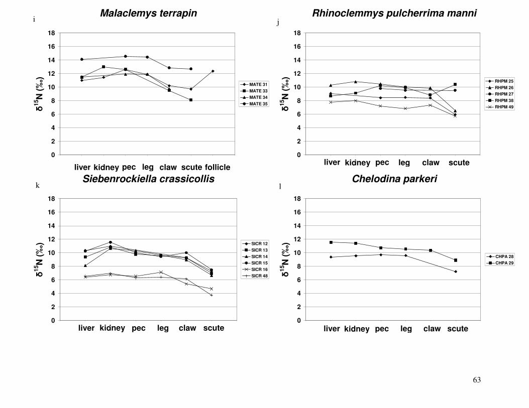
63
i
k
kidney kidney
kidney kidney
Malaclemys terrapin
0
2
4
6
8
10
12
14
16
18
0 1 2 3 4 5 6 7 8
δ15N
(‰
)
MATE 31
MATE 33
MATE 34
MATE 35
Rhinoclemmys pulcherrima manni
0
2
4
6
8
10
12
14
16
18
0 1 2 3 4 5 6 7
δ15N
(‰
)
RHPM 25
RHPM 26
RHPM 27
RHPM 38
RHPM 49
Siebenrockiella crassicollis
0
2
4
6
8
10
12
14
16
18
0 1 2 3 4 5 6 7
δ15N
(‰
) SICR 12
SICR 13
SICR 14
SICR 15
SICR 16
SICR 48
Chelodina parkeri
0
2
4
6
8
10
12
14
16
18
0 1 2 3 4 5 6 7
δ15N
(‰
)
CHPA 28
CHPA 29
j
l
liver pec leg claw scute follicle liver pec leg claw scute
liver pec leg claw scute liver pec leg claw scute
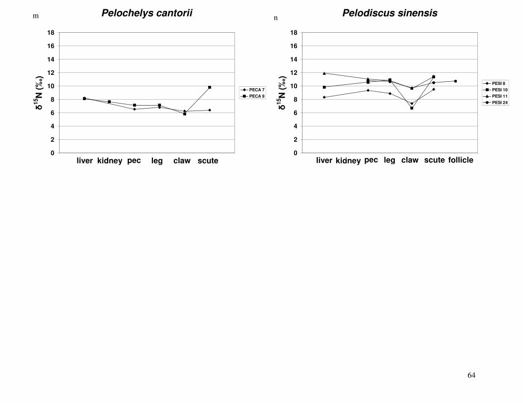
64
m
kidney kidney
Pelochelys cantorii
0
2
4
6
8
10
12
14
16
18
0 1 2 3 4 5 6 7
δ15N
(‰
)
PECA 7
PECA 9
Pelodiscus sinensis
0
2
4
6
8
10
12
14
16
18
0 1 2 3 4 5 6 7 8
δ15N
(‰
)
PESI 8
PESI 10
PESI 11
PESI 24
n
liver pec leg claw scute liver pec leg claw scute follicle
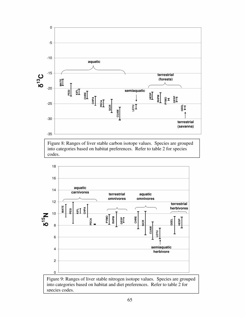
65
-35
-30
-25
-20
-15
-10
-5
0
δ1
3C
aquatic
terrestrial
(forests)
semiaquatic
terrestrial
(savanna)
MA
TE
PE
SI
KIF
L
CH
RE
CH
PA
PE
CA
SIC
R
CU
AM L
EY
U
HE
SP
RH
PM
PY
MO
GE
SP
GE
EL
0
2
4
6
8
10
12
14
16
18
δ1
5N
aquatic
carnivoresterrestrial
omnivores
aquatic
omnivores
terrestrial
herbivores
semiaquatic
herbivore
MA
TE
PE
SI
KIF
L
CH
PA
PE
CA
PY
MO
RH
PM
GE
SP
CH
RE
SIC
R
CU
AM
LE
YU
GE
EL
HE
SP
Figure 8: Ranges of liver stable carbon isotope values. Species are grouped into categories based on habitat preferences. Refer to table 2 for species codes.
Figure 9: Ranges of liver stable nitrogen isotope values. Species are grouped into categories based on habitat and diet preferences. Refer to table 2 for species codes.
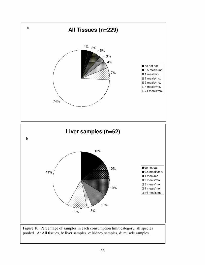
66
All Tissues (n=229)
4% 3%5%
3%
4%
7%
74%
do not eat
0.5 meals/mo.
1 meal/mo.
2 meals/mo.
3 meals/mo.
4 meals/mo.
>4 meals/mo.
a
Liver samples (n=62)
15%
10%
10%
10%
3%11%
41%
do not eat
0.5 meals/mo.
1 meal/mo.
2 meals/mo.
3 meals/mo.
4 meals/mo.
>4 meals/mo.
Figure 10: Percentage of samples in each consumption limit category, all species pooled. A: All tissues, b: liver samples, c: kidney samples, d: muscle samples.
b
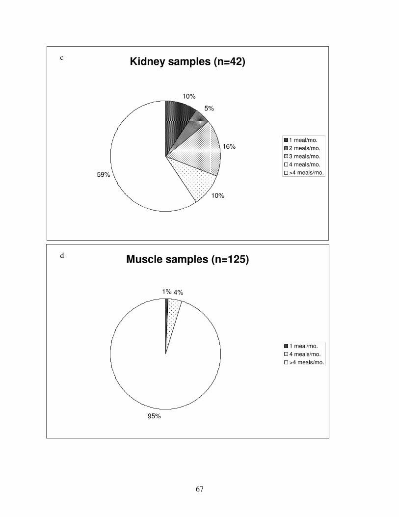
67
Kidney samples (n=42)
10%
5%
16%
10%
59%
1 meal/mo.
2 meals/mo.
3 meals/mo.
4 meals/mo.
>4 meals/mo.
Muscle samples (n=125)
1% 4%
95%
1 meal/mo.
4 meals/mo.
>4 meals/mo.
c
d
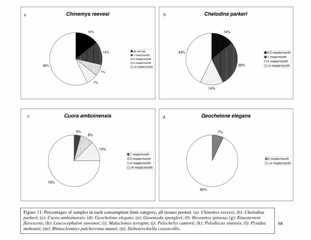
68
a
c
Chinemys reevesi
14%
14%
7%
7%
58%
do not eat
1 meal/month
3 meals/month
4 meals/month
>4 meals/month
Chelodina parkeri
14%
29%
14%
43% 0.5 meals/month
1 meal/month
4 meals/month
>4 meals/month
Cuora amboinensis
4%8%
13%
75%
1 meal/month
3 meals/month
4 meals/month
>4 meals/month
Geochelone elegans
7%
93%
2 meals/month
>4 meals/month
b
d
Figure 11: Percentages of samples in each consumption limit category, all tissues pooled. (a): Chinemys reevesi; (b): Chelodina
parkeri; (c): Cuora amboinensis; (d): Geochelone elegans; (e): Geoemyda spengleri; (f): Heosemys spinosa; (g): Kinosternon
flavescens; (h): Leucocephalon yuwonoi; (i): Malaclemys terrapin; (j): Pelochelys cantorii; (k): Pelodiscus sinensis; (l): Pyxidea
mohoutii; (m): Rhinoclemmys pulcherrima manni; (n): Siebenrockiella crassicollis.
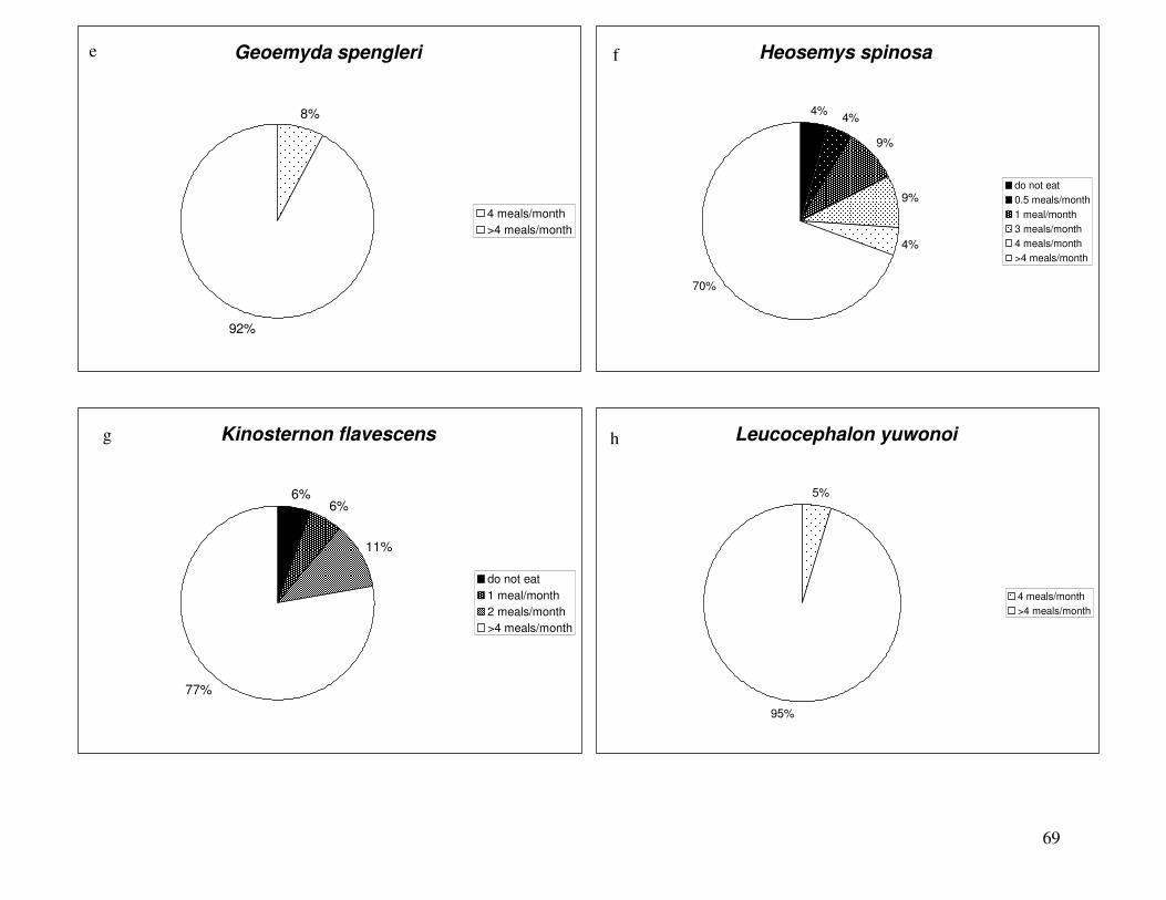
69
e
g
Geoemyda spengleri
8%
92%
4 meals/month
>4 meals/month
Heosemys spinosa
4%4%
9%
9%
4%
70%
do not eat
0.5 meals/month
1 meal/month
3 meals/month
4 meals/month
>4 meals/month
Kinosternon flavescens
6%6%
11%
77%
do not eat
1 meal/month
2 meals/month
>4 meals/month
Leucocephalon yuwonoi
5%
95%
4 meals/month
>4 meals/month
f
h
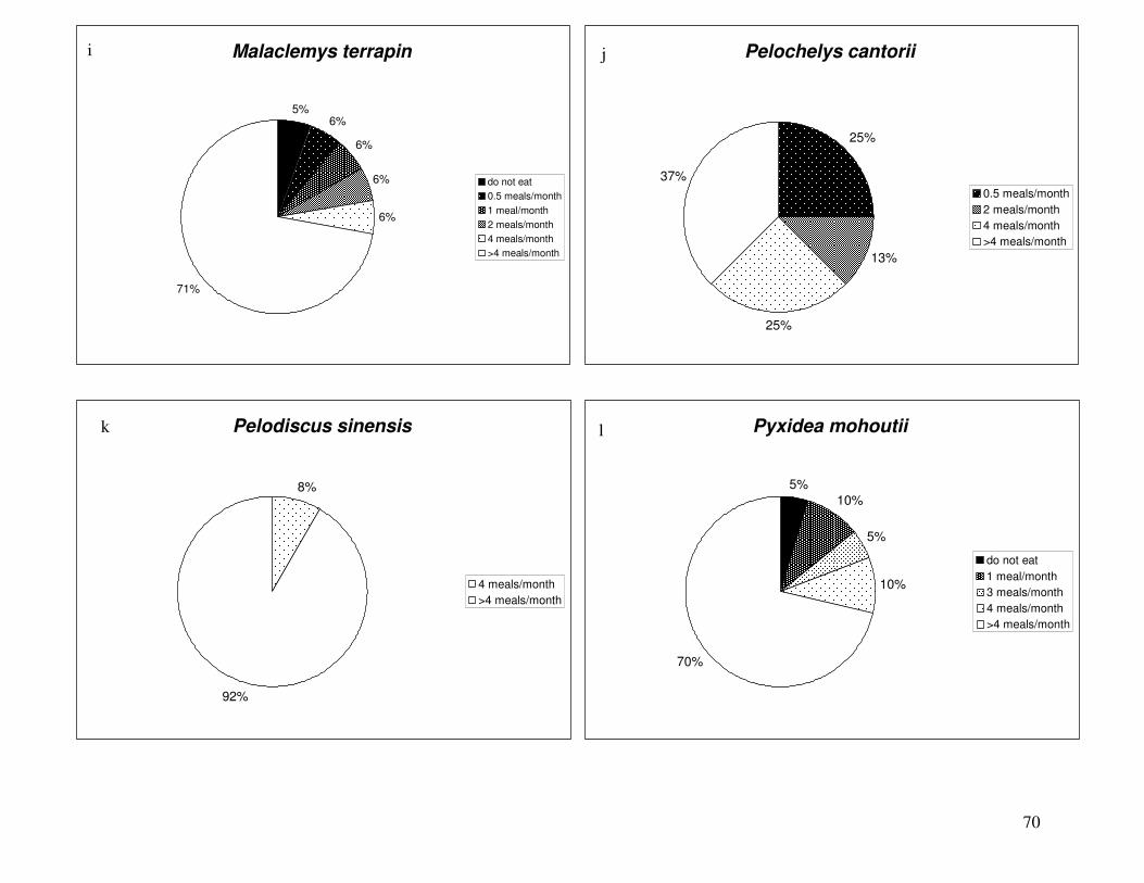
70
i
k
Malaclemys terrapin
5%6%
6%
6%
6%
71%
do not eat
0.5 meals/month
1 meal/month
2 meals/month
4 meals/month
>4 meals/month
Pelochelys cantorii
25%
13%
25%
37%
0.5 meals/month
2 meals/month
4 meals/month
>4 meals/month
Pelodiscus sinensis
8%
92%
4 meals/month
>4 meals/month
Pyxidea mohoutii
5%
10%
5%
10%
70%
do not eat
1 meal/month
3 meals/month
4 meals/month
>4 meals/month
j
l
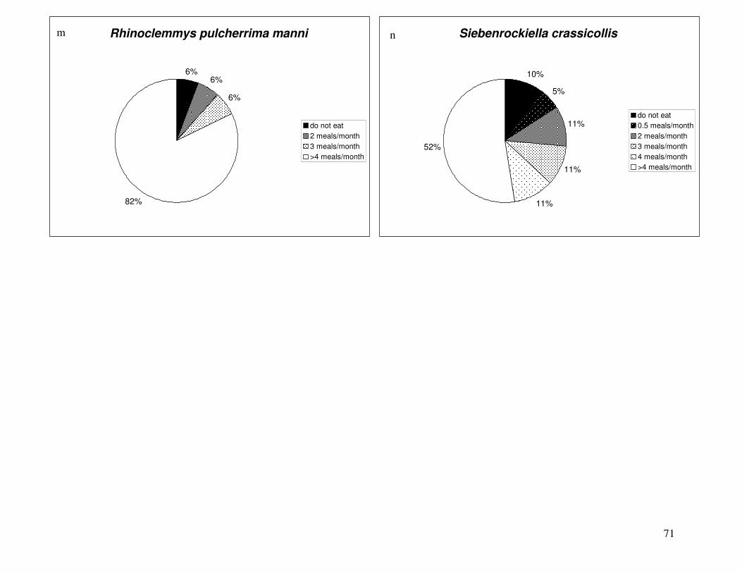
71
m Rhinoclemmys pulcherrima manni
6%6%
6%
82%
do not eat
2 meals/month
3 meals/month
>4 meals/month
Siebenrockiella crassicollis
10%
5%
11%
11%
11%
52%
do not eat
0.5 meals/month
2 meals/month
3 meals/month
4 meals/month
>4 meals/month
n
72
DISCUSSION
Mercury
Tissue distribution:
The general pattern of tissue Hg distribution (liver>kidney≥scutes>muscle) displayed by
the majority of specimens is consistent with past studies of sea turtles (Sakai et al., 1995; Sakai
et al., 2000a; Anan et al., 2001; Day et al., 2005), snapping turtles (Albers et al., 1986; Meyers-
Schone et al., 1993), terrapins (Burger, 2001), and sliders (Meyers-Schone et al., 1993).
Specimens with extremely high liver Hg had Hg levels in all other tissues that were comparable
to those of specimens with relatively low liver Hg. This suggests that, above a certain threshold
of Hg exposure, “excess” Hg accumulates in the liver, while Hg in other tissues remains
relatively low. However, for G. spengleri, it seems as if this excess Hg is allocated to the scutes.
As shown in Figure 2e, scute Hg for this species greatly exceeded Hg in all other tissues,
including liver. This is displayed to a lesser extent in K. flavescens specimens (Figure 2g),
whose liver Hg nearly equaled scute Hg in most specimens. It is interesting that these were also
the two species which had the highest scute Hg concentrations in the entire study. Scute Hg
concentrations that exceed liver Hg concentrations have also been reported in C. caretta (Day et
al., 2005). Scutes are comprised of non-living keratin. Unlike in other tissues, nutrients and
other dietary components allocated to scutes do not return to the total body circulation and are
metabolically unavailable. It is possible that the allocation of excess Hg to the scutes rather than
the liver allows these species to fare better than others in contaminated environments.
Tissues with high metabolic rates, such as liver and kidneys, have shorter nutrient
turnover periods than less metabolically-active tissues, such as muscle, cartilage, and bone. This
73
means that liver cells are replaced more often and reflect more recent dietary components than
do muscle cells.
Differences in Hg among diet groups:
As expected, carnivorous species had significantly greater Hg in most tissues than
omnivorous species, and omnivorous species had significantly greater Hg in most tissues than
herbivorous species. Although the same pattern was detected in liver and kidney samples
(Figure 3) differences in Hg among diet groups were not significantly different for these two
tissue types. Since Hg tends to accumulate in liver and kidneys, they are most sensitive to Hg
contamination. This tendency makes it difficult to detect differences in Hg between diet groups
when species are exposed to a wide spectrum of environmental Hg levels. Tissue Hg
concentrations are influenced by several factors, including trophic position as well as
environmental Hg levels. However, any differences in tissue Hg associated with diet type may
be confounded if some species are obtained from locations with greater levels of contaminants
that others. For example, an omnivore in a highly polluted environment may have higher liver
Hg than a carnivore in a less contaminated habitat. Differences in tissue Hg between dietary
groups are more likely to be detected in muscle, claws, and follicles, which are generally low in
Hg compared to other tissues.
Stable Isotopes
Macronutrients from the diet, including their associated isotopes, can be preferentially
directed into particular tissues before they enter the total body pool of carbon or nitrogen in a
process known as isotopic routing (Martinez del Rio and Wolf, 2005). This results in isotopic
compositions that differ among tissues and between tissues and the diet. Carbon and nitrogen
from the diet is routed through the liver before incorporation into other tissues. As a result, liver
has high carbon and nitrogen turnover rates and its isotopic composition resembles that of the
74
recent diet more closely than less metabolically-active tissues such as muscle and claws (Tieszen
et al., 1983). It was for this reason that only liver δ13C and δ15N values were used to assess
groups of species based on life history traits as shown in Figures 8 and 9. Because tissues differ
in their rates of carbon and nitrogen turnover, analysis of several types of tissues can provide
information on the isotopic composition of the diet at different intervals in the past.
Stable carbon and nitrogen isotope values were analyzed to gain information on carbon
and nitrogen sources. Since we had limited information on the geographic origin of the study
specimens, we also used δ13C and δ15N values along with life history information to develop
hypotheses about the types of environments they occupied. Species were divided into three
groups based on the pattern presented in plots of δ13C values by tissue. Group 1 was
characterized by relatively invariant δ13C values between all tissues. This relationship signifies
that the tissues are in isotopic equilibrium with each other and the diet. This is indicative of an
individual that has remained in a single ecosystem and maintained the same diet for a relatively
long period of time (i.e., several months). Species in group 1 included C. amboinensis, L.
yuwonoi, P. mohoutii, G. elegans, G. spengleri, and K. flavescens. All of the species in this
group, except C. amboinensis, had very narrow ranges in δ15N and δ13C values for tissues, with a
maximum average difference of 2.6‰ between tissues. The low variance of both δ15N and δ13C
between tissues suggests that individuals within a species had similar prey compositions and are
likely from the same population or area.
Group 2 consisted of S. crassicollis, C. reevesi, M. terrapin, R. pulcherrima manni, and
H. spinosa, and was characterized by relatively invariant δ13C values for the internal tissues
(liver, kidney, muscle, and follicles), but a significantly different δ13C value (up to 3.1‰) and
δ15N value (up to 4‰) for the scutes. As stated previously, nutrients in scutes represent dietary
components consumed at the time of scute formation, while nutrients in internal tissues represent
75
more recent dietary items. This suggests that the individuals in group 2 had undergone a recent
dietary change that had not yet been reflected in the scutes at the time of death.
Interestingly, four of the species in group 2 (M. terrapin, C. reevesi, S. crassicollis, and
H. spinosa) also had a bimodal pattern δ15N values, where individuals within the species split
into two or more distinct, nonoverlapping groups for all tissues. These bimodal groups did not
differ in tissue Hg. In the case of both M. terrapin and H. spinosa, one individual was an outlier
in both the carbon and nitrogen isotope compositions, suggesting that these two turtles were
likely from different environments than their conspecifics.
Group 3 included P. sinensis, P. cantorii, and C. parkeri. For these species, there was a
larger difference in δ13C values between tissues within an individual than there was between
species for the other two groups. This suggests that the carbon isotope composition of the tissues
were not in equilibrium with each other or the diet, which may reflect recent dietary changes.
The δ15N values for these species spanned a much narrower range, which may be indicative of
conspecifics that were collected from a single location, but occupying slightly different niches.
In the case of P. cantorii, there is an average difference in δ15N values of 0.4‰ between
individuals, and an average difference of 3.6‰ in δ13C values. This could represent two
individuals from the same river system, with one feeding in a more freshwater environment, and
the other feeding closer to the sea in a more estuarine environment.
Evaluation of Risk to Human Consumers
Comparisons to high Hg fish species:
The EPA advises consumers to avoid eating king mackerel, Gulf of Mexico tilefish,
swordfish, and shark, as they have the highest levels of Hg of all commercial US fish species.
The EPA’s “Mercury Levels in Commercial Fish and Shellfish” (EPA, 2001) lists the mean Hg
concentration of these four species collected from four prior studies as follows: king mackerel,
76
730 ppb; shark, 988 ppb; swordfish, 976 ppb; tilefish, 1,450 ppb. Of all the edible turtle tissue
samples analyzed, 19 of 229 (8.7%) are within or above this range of values.
Comparisons among tissues:
Of the edible tissue types sampled, liver is the riskiest to consume, as it had the highest
proportion of samples in each of the four highest consumption limit categories (do not eat, 0.5
meals/month, 1 meal/month, and 2 meals/month). Liver samples from several popular food trade
species exceeded the 1900 ppb consumption threshold. A single 8 oz. meal of any of these
samples will exceed the reference dose. Frequent consumption of turtles with liver Hg
concentrations that are this high is likely to put consumers at risk for harmful health effects.
Kidneys are less risky to consume than liver, but nearly half (41%) of kidney samples
contained levels of Hg requiring consumption limitations. Muscle samples from all species were
substantially lower in Hg than liver and kidney samples. It is reasonable to assume that
consumers who eat only muscle will be at relatively low risk of harmful health effects due to Hg
exposure. However, turtles are frequently cooked and eaten whole in soups and stews (K.
Buhlmann and C. Hagen, pers. comm.), so it is likely that most consumers will ingest several
types of tissue in one meal.
Comparisons among species:
For ten species (C. amboinensis, G. elegans, G. spengleri, H. spinosa, K. flavescens, L.
yuwonoi, M. terrapin, P. sinensis, P. mohoutii, and R. pulcherrima manni), 70% of the edible
samples (liver, kidney, and muscle) can be safely consumed more than four times per month.
The remaining four species include C. reevesi (58%), S. crassicollis (52%), C. parkeri (43%) and
P. cantorii (37%).
Based on the range of Hg values measured, the proportion of edible samples in each
monthly consumption limit category, and the popularity of the turtles in the food trade, it may be
77
concluded that the turtles with the greatest potential to cause health risks to consumers to include
S. crassicollis, C. reevesi, P. cantorii, C. parkeri, and M. terrapin.
Conclusions
Turtles in this study showed a similar pattern of tissue Hg distribution observed in many
other species of turtles (liver>kidney≥scutes>muscle). Mercury accumulates in the liver and
kidneys, and remains relatively low in muscle tissue. The two species that did not follow this
pattern, G. spengleri and K. flavescens, also displayed the highest scute Hg concentratons in the
entire study. These two species also occupy habitats with a high potential for mercury
contamination. Geoemyda spengleri lives in high-elevation montane forests in southern China,
and is likely exposed to Hg from atmospheric deposition originating from nearby industrial
facilities. This species may also retain its scutes throughout its lifetime instead of shedding
them, which may explain why it had such large scute Hg concentrations. Kinosternon flavescens
aestivates in terrestrial soils, so it may be exposed to Hg not only in its diet, but also from direct
contact with Hg-contaminated sediments. Geoemyda spengleri and K. flavescens may
metabolize Hg differently than the rest of the species in this study, allocating most Hg to their
scutes rather than accumulating it in their livers. This may make these species better able to
handle conditions in a contaminated environment.
As expected, species with more carnivorous diets had higher Hg in all tissues than more
herbivorous species. One species in particular, P. sinensis, had relatively low tissue Hg despite
being piscivorous. Many Chinese softshell turtles are now raised on farms to supply the food
trade, where they are likely fed a diet containing little to no fish. It is possible that the P.
sinensis individuals in this study originated from farms.
Many samples in this study had enough Hg to require consumption limitations according
to EPA standards. A small proportion of all samples contained levels of Hg that were several
78
times higher than the 1900 ppb consumption threshold recommended for most adults. A single
8 oz. meal of a turtle with Hg concentrations such as those measured in the livers of S.
crassicollis or C. reevesi, for example, would exceed the reference dose of 0.1 ppb/day. The
short- and long-term effects of consuming these high levels of Hg are uncertain, but it is clear
that many of the individuals in this study should be consumed very infrequently or not at all.
Although only a small proportion (~6%) of edible tissues sampled were above the recommended
consumption threshold, this study’s sample size of 71 individuals represents an extremely small
percentage of the several million turtles sold for human consumption worldwide. Assuming that
the turtles analyzed here are a representative sample of the total population of food trade turtles,
several hundred thousand turtles on the market may have concentrations of mercury making
them unfit for human consumption. This could signify a troubling public health situation,
although consumers of turtles in Asia are likely to be exposed to Hg from fish and the
environment as well.
This was a reconnaissance study aimed at identifying ranges and patterns of Hg
contamination in food trade turtle species. Conclusions from this study raise several questions
that may be addressed in future research projects. The study specimens consisted of few
individuals from 14 species. There are approximately 310 species of turtles worldwide. To
further investigate the relationship between tissue Hg and certain life history characteristics, such
as body size, sex, and habitat type, a future study would include a higher number of individuals
from one or a few species. Limited location data on the study specimens prevented any
examination of the relationship between environmental Hg levels and tissue Hg levels. To
address this question, a future research project would compare tissue Hg concentrations to Hg
levels in water, soil, and known dietary components from the turtles’ habitats.
79
The majority of the species in this study originated from Asia, with one and two species
respectively from Central America and North America. This impeded a complete analysis of
possible differences in tissue Hg among turtles from different regions. To accurately analyze
any possible regional differences, a future study would contain an equal number of individuals
and species from each region, while controlling for possible confounding factors such as diet.
Revelation of the extremely high tissue Hg concentrations present in some turtles raises the
question of the biological effects of Hg on individual specimens. This question could be
addressed with a study comparing tissue Hg levels with indicators of immune function, such as
plasma lysozyme activity. Several contaminants would have to be analyzed and compared to be
able to accurately attribute any difference in immune function to Hg alone.
Kjellstrom et al. (1986) and Grandjean et al. (1997) were two important public health
studies that linked frequent maternal fish consumption during pregnancy to subtle neurotoxic
effects in children. Replicating these studies with mothers who consumed turtles during
pregnancy would shed light on the health effects of consuming turtles.
Although there is still much to be learned about Hg levels in food trade turtles, greater
public awareness and education about the Hg content of turtles and the possible health
consequences of dietary Hg exposure may help to both protect human consumers and decrease
consumption demand for some turtle species. This may stimulate greater public awareness of the
problem of environmental Hg contamination and encourage citizens to demand greater
restrictions on Hg emissions. This may also help to relax pressure on turtle populations suffering
from extensive harvesting for the food trade.
80
REFERENCES
Albers, P. H., L. Sileo, and B. M. Mulhern. 1986. "Effects of environmental contaminants on
snapping turtles of a tidal wetland." Archives of Environmental Contamination and
Toxicology 15: 39-49.
Al-Saleh, I. and N. Shinwari. 2001. "Report on the levels of cadmium, lead, and mercury in
imported rice grain samples." Biological Trace Element Research 83: 91-96.
Altherr, S. and D. Freyer. 2000. "Asian turtles are threatened by extinction." Turtle and Tortoise
Newsletter (1): 7-11.
Anan, Y., T. Kunito, I. Watanabe, H. Sakai, and S. Tanabe. 2001. "Trace element accumulation
in hawksbill turtles (Eretmochelys imbricata) and green turtles (Chelonia mydas) from
Yaeyama Islands, Japan." Environmental Toxicology and Chemistry 20(12): 2802-2814.
Artner, H. and A. Hofer. 2001. "Observations in the Qing Ping Free Market, Guangzhou, China,
November 2000." Turtle and Tortoise Newsletter (3): 14.
Ashpole, S. A., C. A. Bishop, and R. J. Brooks. 2004. "Contaminant residues in snapping turtle
(Chelydra s. serpentina) eggs from the Great Lakes-St. Lawrence River basin (1999 to
2000)." Archives of Environmental Contamination and Toxicology 47: 240-252.
Barrie, A. and S. J. Prosser. 1996. “Automated analysis of light-element stable isotopes by
isotope ratio mass spectrometry.” In: Boutton, T. W. and S. Yamasaki (eds.) Mass
Spectometry. Marcel Dekker: New York, pp 1-46.
Becker, P. H. 1992. "Egg mercury levels decline with the laying sequence in Charadriliformes."
Bulletin of Environmental Contamination and Toxicology 48: 762-767.
81
Behler, J. L. 1997. “Troubled times for turtles”. International Conference on Conservation,
Restoration, and Management of Turtles and Tortoises.
Bishop, C. A., R. J. Brooks, J. H. Carey, P. Ng, R. J. Norstrom, and D. R. S. Lean. 1991. "The
case for a cause-effect linkage between environmental contamination and development in
eggs of the common snapping turtle (Chelydra s. serpentina) from Ontario, Canada."
Journal of Toxicology and Environmental Health 33: 521-547.
Blanvillain, G., J. A. Schwenter, R. D. Day, D. Point, S. J. Christopher, W. A. Roumillat, and D.
W. Owens. 2007. “Diamondback terrapins, Malaclemys terrapin, as a sentinel species for
monitoring mercury pollution of estuarine ecosystems in South Carolina and Georgia,
USA.” Environmental Toxicology and Chemistry 26(7): 1441-1450.
Boening, D. W. 2000. "Ecological effects, transport, and fate of mercury: a general review."
Chemosphere 40: 1355-1351.
Bonin, F., B. Deveaux, and A. Dupre. (2006). Turtles of the World. Johns Hopkins University
Press: Baltimore.
Bonin, J., J.-L. DesGranges, C. A. Bishop, J. Rodrigue, A. Gendron, and J. E. Elliot. 1995.
"Comparative study of contaminants in the mudpuppy (Amphibia) and the common snapping
turtle (Reptilia), St. Lawrence River, Canada." Archives of Environmental Contamination
and Toxicology 28: 184-194.
Bouton, S. N., P. C. Frederick, M. G. Spalding, and H. McGill. 1999. "Effects of chronic, low
concentrations of dietary methylmercury on the behavior of juvenile great egrets."
Environmental Toxicology and Chemistry 18(9): 1934-1939.
Burger, J. 2002. "Metals in tissues of diamondback terrapin from New Jersey." Environmental
Monitoring and Assessment 77: 255-263.
82
Burger, J. and J. W. Gibbons. 1998. "Trace elements in egg contents and eggshells of slider
turtles (Trachemys scripta) from the Savannah River Site." Archives of Environmental
Contamination and Toxicology 34: 382-386.
Carr, A. (1952). Handbook of Turtles. Cornell University Press: Ithaca and London.
Coplen, T. B. 1996. "New guidelines for reporting stable hydrogen, carbon, and oxygen
isotope-ratio data." Geochim Cosmochim Acta 60: 3359-3360.
Craig, H. 1957. "Isotopic standards for carbon and oxygen and correlation factors for mass-
spectrometric analysis of carbon dioxide." Geochim Cosmochim Acta 12: 133-149.
Dansereau, M., N. Lariviere, D. Du Tremblay, and D. Belanger. 1999. "Reproductive
performance of two generations of female semidomesticated mink fed diets containing
organic mercury contaminated freshwater fish." Archives of Environmental Contamination
and Toxicology 36: 221-226.
Davenport, J. and J. Wrench. 1990. "Metal levels in a leatherback turtle." Marine Pollution
Bulletin 21(1): 40-41.
Day, R. D., S. J. Christopher, P. R. Becker, and D. W. Whitaker. 2005. "Monitoring mercury in
the loggerhead sea turtle, Caretta caretta." Environmental Science and Technology 39: 437-
446.
DesGranges, J.-L., J. Rodrigue, B. Tardiff, and M. Laperle. 1998. "Mercury accumulation and
biomagnification in ospreys (Pandion haliaetus) in the James Bay and Hudson Bay regions
of Quebec." Archives of Environmental Contamination and Toxicology 35: 330-341.
Drasch, G., S. Bose-O'Reilly, C. Beinhoff, G. Roider, and S. Maydl. 2001. "The Mt. Diwata
study on the Philippines 1999--assessing mercury intoxication of the population by small
scale gold mining." Science of the Total Environment 267: 151-168.
83
Evers, D. C. 2005. “Mercury connections: The extent and effects of mercury pollution in
northeastern North America”. Biodiversity Research Institute: 28.
Evers, D. C., K. M. Taylor, A. Major, R. J. Taylor, R. H. Poppenga, and A. M. Scheuhammer.
2003. "Common loon eggs as indicators of methylmercury availability in North America."
Ecotoxicology 12: 69-81.
Finkelman, R. B., H. E. Belkin, and B. Zhang. 1999. “Health impacts of domestic coal use in
China”. National Academy of Sciences colloquium on Geology, Minerology, and Human
Welfare. Irvine, CA.
Friedmann, A. S., M. C. Watzin, T. Brinck-Johnsen, and J. C. Leiter. 1996. "Low levels of
dietary methylmercury inhibit growth and gonadal development in juvenile walleye
(Stizostedion vitreum)." Aquatic Toxicology 35: 265-278.
Gibbons, J. W. 1967. "Variation in growth rates in three populations of the painted turtle,
Chrysemys picta." Herpetologica 23(4): 296-303.
Gibbons, J. W. 1968. "Carapacial algae in a population of the painted turtle, Chrysemys picta."
American Midland Naturalist 79(2): 57-519.
Gibbons, J. W., D. E. Scott, T. J. Ryan, K. A. Buhlmann, T. D. Tuberville, B. S. Metts, J. L.
Greene, T. Mills, Y. Leiden, S. Poppy, and C. T. Winne. 2000. "The global decline of
reptiles, deja vu amphibians." Bioscience 50(8): 653-666.
Gibbons, J. W. and D. W. Tinkle. 1969. "Reproductive variation between turtle populations in a
single geographic area." Ecology 50(2): 340-341.
Gibbons, J. W., J. E. Lovich, Tucker, A. D., FitzSimmons, N. N., and J. L. Greene. 2001.
"Demographic and ecological factors affecting conservation and management of the
diamondback terrapin (Malaclemys terrapin) in South Carolina." Chelonian Conservation
and Biology 4(1): 66-74.
84
Godley, B. J., D. R. Thompson, and R. W. Furness. 1999. "Do heavy metal concentrations pose
a threat to marine turtles from the Mediterranean Sea?" Marine Pollution Bulletin 38(6): 497-
502.
Golet, W. A. and T. A. Haines. 2001. "Snapping turtles (Chelydra serpentina) as monitors for
mercury contamination of aquatic environments." Environmental Monitoring and
Assessment 71: 211-220.
Gordon, A. N., A. R. Pople, and J. Ng. 1998. "Trace metal concentrations in livers and kidneys
of sea turtles from south-eastern Queensland, Australia." Marine and Freshwater Research
49: 409-414.
Grandjean, P., P. Weihe, P. J. Jorgensen, T. Clarkson, E. Cernichiari, and T. Videro. 1992.
"Impact of maternal seafood diet on fetal exposure to mercury, selenium, and lead." Archives
of Environmental Health 47(3): 185-195.
Grandjean, P., P. Weihe, R. F. White, and F. Debes. 1998. "Cognitive performance of children
prenatally exposed to "safe" levels of methylmercury." Environmental Research, Section A
77: 165-172.
Grandjean, P., P. Weihe, R. F. White, F. Debes, S. Araki, K. Yokoyama, K. Murata, N.
Sorensen, R. Dahl, and P. Jorgensen. 1997. "Cognitive deficit in 7-year old children with
prenatal exposure to methylmercury." Neurotoxicology and Teratology 19(6): 417-428.
Hagen, C. and I. Y. S. Ching. 2005. "Distribution, natural history, and exploitation of
Leucocephalon yuwonoi in Central Sulawesi, Indonesia." Chelonian Conservation and
Biology 4(4): 948-951.
Haitao, S. 2000. "Results of turtle market surveys in Chengdu and Kunming." Turtle and
Tortoise Newsletter (6): 15b-16.
85
Haitao, S. 2004. "Observations of wildlife trade in Wengchang City, Hainan Island, China."
Turtle and Tortoise Newsletter (8): 12-13.
Hammerschmidt, C. R., M. B. Sandheinrich, J. G. Weiner, and R. G. Rada. 2002. "Effects of
dietary methylmercury on reproduction of fathead minnows." Environmental Science and
Technology 36: 877-883.
Hammerschmidt, C. R., J. G. Wiener, B. E. Frasier, R. G. 1999. "Methlymercury content of eggs
in yellow perch related to maternal exposure in four Wisconsin lakes." Environmental
Science and Technology 33: 999-1003.
Heinz, G. H. 1979. "Methylmercury: Reproductive and behavioral effects on three generations
of mallard ducks." Journal of Wildlife Management 43(2): 394-401.
Helwig, D. D. and M. E. Hora. 1983. "Polychlorinated biphenyl, mercury, and cadmium
concentrations in Minnesota snapping turtles." Bulletin of Environmental Contamination and
Toxicology 30: 186-190.
Horvat, M., N. Nolde, V. Fajon, V. Jereb, M. Logar, S. Lojen, R. Jacimovic, I. Falnoga, Q. Liya,
J. Faganeli, and D. Drobne. 2003. "Total mercury, methylmercury, and selenium in mercury
polluted areas in the province Guizhou, China." Science of the Total Environment 304: 231-
256.
Hudson, R. and K. Buhlmann. 2000. "Turtle Rescue--Turtle Survival Alliance Executive
Summary." Turtle and Tortoise Newsletter (6): 6-12.
Iskandar, D. T. (2000). Turtles and Crocodiles of Insular Southeast Asia and New Guinea.
PALMedia Citra: Badung.
Jagoe, C. H., B. Arnold-Hill, G. B. Yanochko, P. V. Winger, and I. L. Brisbin. 1998. "Mercury
in alligators (Alligator missisippiensis) in the southeastern United States." Science of the
Total Environment 213: 255-262.
86
Klemens, M. W. (ed.) (2000). Turtle Conservation. Smithsonian Institution Press: Washington,
D. C. and London.
Knight, A. W. and J. W. Gibbons. 1968. "Food of the painted turtle, Chrysemys picta, in a
polluted river." American Midland Naturalist 80(2): 558-562.
Lovich, J. E., R. A. Mittermeier, P. C. H. Pritchard, A. G. J. Rhodin, and J. W. Gibbons. 2000.
"Powdermill Conference: Trouble for the world's turtles." Turtle and Tortoise Newsletter (1):
16-17.
Luiselli, L., G. C. Akani, and E. Politano. 2006. "Effects of habitat alteration caused by
petrochemical activities and oil spills on the habitat use and interspecific relationships among
four species of Afrotropical freshwater turtles." Biodiversity and Conservation 15: 3751-
3767.
Mariotti, A. 1983. "Atmospheric nitrogen is a reliable standard for natural 15N abundance
measurements." Nature 303: 685-687.
Martinez del Rio, C. and B. O. Wolf. 2005. “Mass-Balance Models for Animal Isotopic
Ecology”. In: Stark, J. M. and T. Wang (eds.) Physiological and Ecological Adaptations to
Feeding in Vertebrates. Science Publishers: Enfield, NH.
McCord, W. 2000. "Current review on China food market/turtle crisis." Turtle and Tortoise
Newsletter (1): 13-14.
Menasveta, P. and V. Cheevaparanapiwat. 1981. "Heavy metals, organochlorine pesticides, and
PCBs in green mussels, mullets, and sediments of river mouths in Thailand." Marine
Pollution Bulletin 12(1): 19-25.
Menasveta, P., V. Cheevaparanapiwat, and C. Wongwit. 1985. "Heavy metals in bivalves
collected from river estuaries of Thailand." Asian Marine Biology 2: 31-36.
87
Meyer, M., D. C. Evers, J. J. Hatigan, and P. S. Rasmussen. 1998. "Patterns of common loon
(Gavia immer) mercury exposure, reproduction, and survival in Wisconsin, USA."
Environmental Toxicology and Chemistry 17(2): 184-190.
Meyers-Schone, L., L. R. Shugart, J. J. Beauchamp, and B. T. Walton. 1993. "Comparison of
two freshwater turtle species as monitors of radionuclide and chemical contamination: DNA
damage and residue analysis." Environmental Toxicology and Chemistry 12: 1487-1496.
Meyers-Schone, L. and B. T. Walton. 1994. "Turtles as monitors of chemical contaminants in
the environment." Reviews of Environmental Contamination and Toxicology 135: 93-153.
Mierle, G., E. M. Addison, K. S. Macdonald, and D. G. Joachim. (2000). "Mercury levels in
tissues of otters from Ontario, Canada: Variation with age, sex, and location." Environmental
Toxicology and Chemistry 19(12): 3044-3051.
National Research Council. (2000). Toxicological Effects of Methylmercury. National Academy
Press: Washington, DC.
Pasha, M. K. S., B. Wright, and T. Joseph. 2004. "Scale and distribution of trade in chelonians
in India." Turtle and Tortoise Newsletter (8): 14-16.
Pinnegar, J. K. and N. V. C. Polunin. 1999. "Differential fractionation of δ13C and δ15N among
fish tissues: Implications for the study of trophic interactions." Functional Ecology 13: 225-
231.
Redmayne, A. C., J. P. Kim, G. P. Closs, and K. A. Hunter. 2000. "Methyl mercury
bioaccumulation in long-finned eels, Anguilla dieffenbachii, from three rivers in Otago, New
Zealand." Science of the Total Environment 262: 27-37.
Sakai, H., K. Saeki, H. Ichihashi, N. Kamezaki, S. Tanabe, and R. Tatsukawa. 2000a. "Growth-
related changes in heavy metal accumulation in green turtle (Chelonia mydas) from Yaeyama
88
Islands, Okinawa, Japan." Archives of Environmental Contamination and Toxicology 39:
378-385.
Sakai, H., K. Saeki, H. Ichihashi, H. Suganuma, S. Tanabe, and R. Tatsukawa. 2000b. "Species-
specific distribution of heavy metals in tissues and organs of loggerhead turtle (Caretta
caretta) and green turtle (Chelonia mydas) from Japanese coastal waters." Marine Pollution
Bulletin 40(8): 701-709.
Sakai, H., H. Ichihashi, H. Suganuma, and R. Tatsukawa. 1995. "Heavy metal monitoring in sea
turtles using eggs." Marine Pollution Bulletin 30(5): 347-353.
Scheuhammer, A. M., C. M. Atchison, A. H. K. Wong, and D. C. Evers. 1998. "Mercury
exposure in breeding common loons (Gavia immer) in Central Ontario, Canada."
Environmental Toxicology and Chemistry 17(2): 191-196.
Scheuhammer, A. M., A. H. K. Wong, and D. Bond. 1998. "Mercury and selenium
accumulation in common loons (Gavia immer) and common mergansers (Mergus merganser)
from Eastern Canada." Environmental Toxicology and Chemistry 17(2): 197-201.
Schwarcz, H. P. 1991. "Some theoretical aspects of isotope paleodiet studies." Journal of
Archaeological Science 18: 261-275.
Shi, H. and J. F. Parham. 2001. "Preliminary observations of a large turtle farm in Hainan
Province, People Republic of China." Turtle and Tortoise Newsletter (3): 4-6.
Spalding, M. G., P. C. Frederick, H. McGill, S. N. Bouton, L. J. Richley, I. M. Schumacher, C.
G. M. Blackmore, and J. Harrison. 2000. "Histologic, neurologic, and immunologic effects
of methylmercury in captive great egrets." Journal of Wildlife Diseases 36(3): 423-435.
Stone, W. B., E. Kiviat, and S. A. Butkas. 1980. "Toxicants in snapping turtles." New York Fish
and Game Journal 27(1): 39-50.
89
Stoneburner, D. L., M. N. Nicora, and E. R. Blood. 1980. "Heavy metals in loggerhead sea turtle
eggs (Caretta caretta): Evidence to support the hypothesis that demes exist in the Western
Atlantic population." Journal of Herpetology 14(2): 171-175.
Storelli, M. M., E. Ceci, and G. O. Marcotrigiano. 1998. "Comparison of total mercury,
methylmercury, and selenium in muscle tissues and in the liver of Stenella coeruleoalba
(Meyen) and Caretta caretta (Linnaeus)." Bulletin of Environmental Contamination and
Toxicology 61: 541-547.
Storelli, M. M. and G. O. Marcotrigiano. 2003. "Heavy metal residues in tissues of marine
turtles." Marine Pollution Bulletin 46: 397-400.
Storelli, M. M., E. Ceci, and G. O. Marcotrigiano. 1998. "Distribution of heavy metal residues
in some tissues of Caretta caretta (Linnaeus) specimen beached along the Adriatic Sea
(Italy)." Bulletin of Environmental Contamination and Toxicology 60: 546-552.
Struger, J. 1993. "Environmental contaminants in eggs of the common snapping turtle (Chelydra
s. serpentina) from the Great Lakes-St. Lawrence River basin of Ontario, Canada (1981-
1984)." Journal of Great Lakes Research 19(4): 681-694.
Suckcharoen, S., P. Nuorteva, and E. Hasanen. 1978. "Alarming signs of mercury pollution in a
freshwater area of Thailand." Ambio 7: 113-116.
Sundar, K. S. G. 2004. "From a poacher's bag: Patterns of exploitation of Lissemys punctata
andersoni in Etawah, Uttar Pradesh, India." Turtle and Tortoise Newsletter (8): 18-19.
Swartz, C. D., K. C. Donnelly, A. Islamzadeh, G. T. Rowe, W. J. Rogers, G. M. Palatnikov, A.
A. Mekhtiev, R. Kasimov, T. J. McDonald, J. K. Wickliffe, B. J. Presley, and J. W. Bickham.
2003. "Chemical contaminants and their effects in fish and wildlife from the industrial zone
of Sumgayit, Republic of Azerbaijan." Ecotoxicology 12: 509-521.
90
Tieszen, L. L., T. W. Boutton, K. G. Tesdahl, and N. A. Slade. 1983. "Fractionation and
turnover of stable carbon isotopes in animal tissues: Implications for δ13C analysis of diet."
Oecologia 57: 32-37.
Tucker, A. D., N. N. FitzSimmons, and J. W. Gibbons. 1995. "Resource partitioning by the
estuarine turtle Malaclemys terrapin: Trophic, spatial, and temporal foraging constraints."
Herpetologica 51(2): 167-181.
Turtle Conservation Fund. (2002). A Global Action Plan for Conservation of Tortoises and
Freshwater Turtles. Strategy and Funding Prospectus 2002-2007. Conservation International
and Chelonian Research Foundation: Washington, DC, 30 pp.
U. S. Environmental Protection Agency. 1998. “EPA Method 7473: Mercury in solids and
solutions by thermal decomposition, amalgamation, and atomic absorption
spectrophotometry.”
U. S. Environmental Protection Agency (2000). Guidance for Assessing Chemical Contaminant
Data for Use in Fish Advisories. Volume 2: Risk Assessment and Fish Consumption Limits.
U. S. Environmental Protection Agency and U. S. Department of Health and Human Services
(2001). “Mercury Levels in Commercial Fish and Shellfish.”
U. S. Environmental Protection Agency and U. S. Department of Health and Human Services
(2004). “What You Need to Know About Mercury in Fish and Shellfish.”
van Dijk, P. P., B. L. Stuart, and A. G. J. Rhodin (eds.). 2000. "Asian Turtle Trade: Proceedings
of a Workshop on Conservation and Trade of Freshwater Turtles and Tortoises in Asia."
Chelonian Research Monographs 2.
Wang, Q., D. Kim, D. Dionysios, G. A. Sorial, and D. Timberlake. 2004. "Sources and
remediation for mercury contamination in aquatic systems--a literature review."
Environmental Pollution 131: 323-336.
91
Webber, H. M. and T. A. Haines. 2003. "Mercury effects on predator avoidance behavior of a
forage fish, golden shiner (Notemigonus crysoleucas)." Environmental Toxicology and
Chemistry 22(7): 1556-1561.
Weihe, P., P. Grandjean, F. Debes, and R. F. White. 1996. "Health implications for Faroe
Islanders of heavy metals and PCBs from pilot whales." Science of the Total Environment
186: 141-148.
Williams, W. 1999. "The deadly shell game." Animals 132(3): 16-22.
Wolfe, M. F., S. Schwarzbach, and R. A. Sulaiman. 1998. "Effects of mercury on wildlife: A
comprehensive review." Environmental Toxicology and Chemistry 17(2): 146-160.
Xianlin, M., Z. Zhihua, and B. L. Stuart. 2002. "Recent actions by the People's Republic of
China to better control international trade of turtles." Turtle and Tortoise Newsletter: 15.
Xiao, Z., J. Sommar, and O. Lindqvist. 1998. "Atmospheric mercury deposition on Fanjing
Mountain Nature Reserve, Guizhou, China." Chemosphere 36(10): 2191-2200.
Yanochko, G. M., C. H. Jagoe, and I. L. Brisbin, Jr. 1997. "Tissue mercury concentrations in
alligators (Alligator mississippiensis) from the Florida Everglades and Savannah River Site,
South Carolina." Archives of Environmental Contamination and Toxicology 32: 323-328.
Yoshinaga, J., T. Suzuki, T. Hongo, M. Minagawa, R. Ohtsuka, T. Kawabe, T. Inaoka, and T.
Akimichi. 1992. "Mercury concentration correlates with nitrogen stable isotope ratio in the
animal food of Papuans." Ecotoxicology and Environmental Safety 24: 37-45.
Zingde, M. D. and B. N. Desai. 1981. "Mercury in Thana Creek, Bombay Harbor." Mercury
Pollution Bulletin 12(7): 237-241
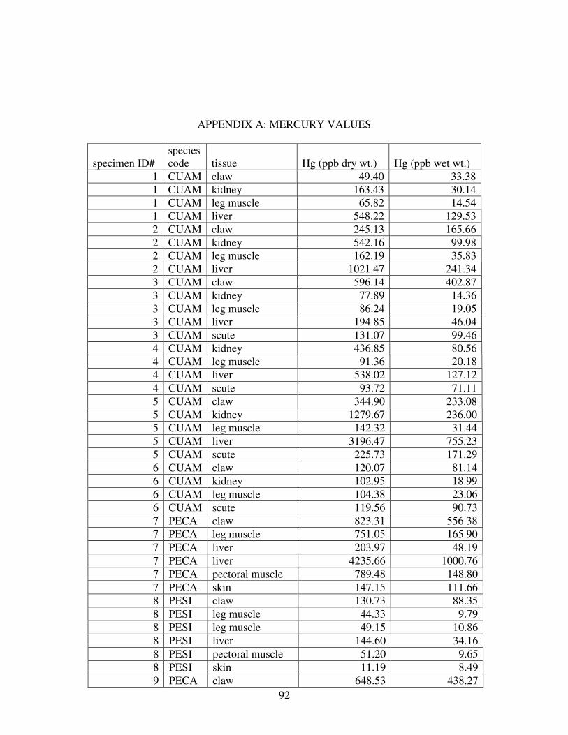
92
APPENDIX A: MERCURY VALUES
specimen ID# species code tissue Hg (ppb dry wt.) Hg (ppb wet wt.)
1 CUAM claw 49.40 33.38
1 CUAM kidney 163.43 30.14
1 CUAM leg muscle 65.82 14.54
1 CUAM liver 548.22 129.53
2 CUAM claw 245.13 165.66
2 CUAM kidney 542.16 99.98
2 CUAM leg muscle 162.19 35.83
2 CUAM liver 1021.47 241.34
3 CUAM claw 596.14 402.87
3 CUAM kidney 77.89 14.36
3 CUAM leg muscle 86.24 19.05
3 CUAM liver 194.85 46.04
3 CUAM scute 131.07 99.46
4 CUAM kidney 436.85 80.56
4 CUAM leg muscle 91.36 20.18
4 CUAM liver 538.02 127.12
4 CUAM scute 93.72 71.11
5 CUAM claw 344.90 233.08
5 CUAM kidney 1279.67 236.00
5 CUAM leg muscle 142.32 31.44
5 CUAM liver 3196.47 755.23
5 CUAM scute 225.73 171.29
6 CUAM claw 120.07 81.14
6 CUAM kidney 102.95 18.99
6 CUAM leg muscle 104.38 23.06
6 CUAM scute 119.56 90.73
7 PECA claw 823.31 556.38
7 PECA leg muscle 751.05 165.90
7 PECA liver 203.97 48.19
7 PECA liver 4235.66 1000.76
7 PECA pectoral muscle 789.48 148.80
7 PECA skin 147.15 111.66
8 PESI claw 130.73 88.35
8 PESI leg muscle 44.33 9.79
8 PESI leg muscle 49.15 10.86
8 PESI liver 144.60 34.16
8 PESI pectoral muscle 51.20 9.65
8 PESI skin 11.19 8.49
9 PECA claw 648.53 438.27
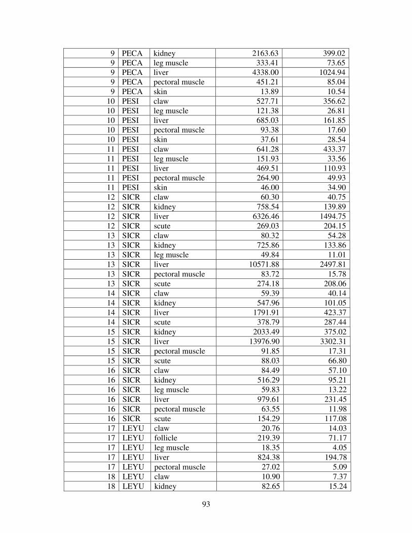
93
9 PECA kidney 2163.63 399.02
9 PECA leg muscle 333.41 73.65
9 PECA liver 4338.00 1024.94
9 PECA pectoral muscle 451.21 85.04
9 PECA skin 13.89 10.54
10 PESI claw 527.71 356.62
10 PESI leg muscle 121.38 26.81
10 PESI liver 685.03 161.85
10 PESI pectoral muscle 93.38 17.60
10 PESI skin 37.61 28.54
11 PESI claw 641.28 433.37
11 PESI leg muscle 151.93 33.56
11 PESI liver 469.51 110.93
11 PESI pectoral muscle 264.90 49.93
11 PESI skin 46.00 34.90
12 SICR claw 60.30 40.75
12 SICR kidney 758.54 139.89
12 SICR liver 6326.46 1494.75
12 SICR scute 269.03 204.15
13 SICR claw 80.32 54.28
13 SICR kidney 725.86 133.86
13 SICR leg muscle 49.84 11.01
13 SICR liver 10571.88 2497.81
13 SICR pectoral muscle 83.72 15.78
13 SICR scute 274.18 208.06
14 SICR claw 59.39 40.14
14 SICR kidney 547.96 101.05
14 SICR liver 1791.91 423.37
14 SICR scute 378.79 287.44
15 SICR kidney 2033.49 375.02
15 SICR liver 13976.90 3302.31
15 SICR pectoral muscle 91.85 17.31
15 SICR scute 88.03 66.80
16 SICR claw 84.49 57.10
16 SICR kidney 516.29 95.21
16 SICR leg muscle 59.83 13.22
16 SICR liver 979.61 231.45
16 SICR pectoral muscle 63.55 11.98
16 SICR scute 154.29 117.08
17 LEYU claw 20.76 14.03
17 LEYU follicle 219.39 71.17
17 LEYU leg muscle 18.35 4.05
17 LEYU liver 824.38 194.78
17 LEYU pectoral muscle 27.02 5.09
18 LEYU claw 10.90 7.37
18 LEYU kidney 82.65 15.24
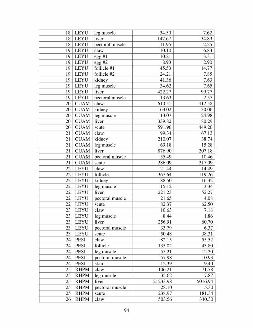
94
18 LEYU leg muscle 34.50 7.62
18 LEYU liver 147.67 34.89
18 LEYU pectoral muscle 11.95 2.25
19 LEYU claw 10.10 6.83
19 LEYU egg #1 10.21 3.31
19 LEYU egg #2 8.93 2.90
19 LEYU follicle #1 45.53 14.77
19 LEYU follicle #2 24.21 7.85
19 LEYU kidney 41.36 7.63
19 LEYU leg muscle 34.62 7.65
19 LEYU liver 422.27 99.77
19 LEYU pectoral muscle 13.63 2.57
20 CUAM claw 610.51 412.58
20 CUAM kidney 163.02 30.06
20 CUAM leg muscle 113.07 24.98
20 CUAM liver 339.82 80.29
20 CUAM scute 591.96 449.20
21 CUAM claw 99.34 67.13
21 CUAM kidney 210.07 38.74
21 CUAM leg muscle 69.18 15.28
21 CUAM liver 876.90 207.18
21 CUAM pectoral muscle 55.49 10.46
21 CUAM scute 286.09 217.09
22 LEYU claw 21.44 14.49
22 LEYU follicle 367.64 119.26
22 LEYU kidney 88.50 16.32
22 LEYU leg muscle 15.12 3.34
22 LEYU liver 221.23 52.27
22 LEYU pectoral muscle 21.65 4.08
22 LEYU scute 82.37 62.50
23 LEYU claw 10.63 7.18
23 LEYU leg muscle 8.44 1.86
23 LEYU liver 256.91 60.70
23 LEYU pectoral muscle 33.79 6.37
23 LEYU scute 50.48 38.31
24 PESI claw 82.15 55.52
24 PESI follicle 135.02 43.80
24 PESI leg muscle 55.21 12.20
24 PESI pectoral muscle 57.98 10.93
24 PESI skin 12.39 9.40
25 RHPM claw 106.21 71.78
25 RHPM leg muscle 35.62 7.87
25 RHPM liver 21233.98 5016.94
25 RHPM pectoral muscle 28.10 5.30
25 RHPM scute 238.97 181.34
26 RHPM claw 503.56 340.30
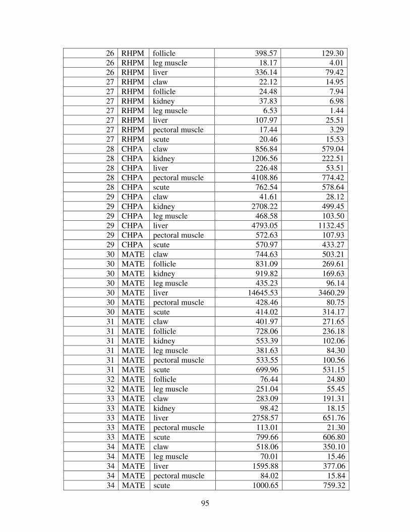
95
26 RHPM follicle 398.57 129.30
26 RHPM leg muscle 18.17 4.01
26 RHPM liver 336.14 79.42
27 RHPM claw 22.12 14.95
27 RHPM follicle 24.48 7.94
27 RHPM kidney 37.83 6.98
27 RHPM leg muscle 6.53 1.44
27 RHPM liver 107.97 25.51
27 RHPM pectoral muscle 17.44 3.29
27 RHPM scute 20.46 15.53
28 CHPA claw 856.84 579.04
28 CHPA kidney 1206.56 222.51
28 CHPA liver 226.48 53.51
28 CHPA pectoral muscle 4108.86 774.42
28 CHPA scute 762.54 578.64
29 CHPA claw 41.61 28.12
29 CHPA kidney 2708.22 499.45
29 CHPA leg muscle 468.58 103.50
29 CHPA liver 4793.05 1132.45
29 CHPA pectoral muscle 572.63 107.93
29 CHPA scute 570.97 433.27
30 MATE claw 744.63 503.21
30 MATE follicle 831.09 269.61
30 MATE kidney 919.82 169.63
30 MATE leg muscle 435.23 96.14
30 MATE liver 14645.53 3460.29
30 MATE pectoral muscle 428.46 80.75
30 MATE scute 414.02 314.17
31 MATE claw 401.97 271.65
31 MATE follicle 728.06 236.18
31 MATE kidney 553.39 102.06
31 MATE leg muscle 381.63 84.30
31 MATE pectoral muscle 533.55 100.56
31 MATE scute 699.96 531.15
32 MATE follicle 76.44 24.80
32 MATE leg muscle 251.04 55.45
33 MATE claw 283.09 191.31
33 MATE kidney 98.42 18.15
33 MATE liver 2758.57 651.76
33 MATE pectoral muscle 113.01 21.30
33 MATE scute 799.66 606.80
34 MATE claw 518.06 350.10
34 MATE leg muscle 70.01 15.46
34 MATE liver 1595.88 377.06
34 MATE pectoral muscle 84.02 15.84
34 MATE scute 1000.65 759.32
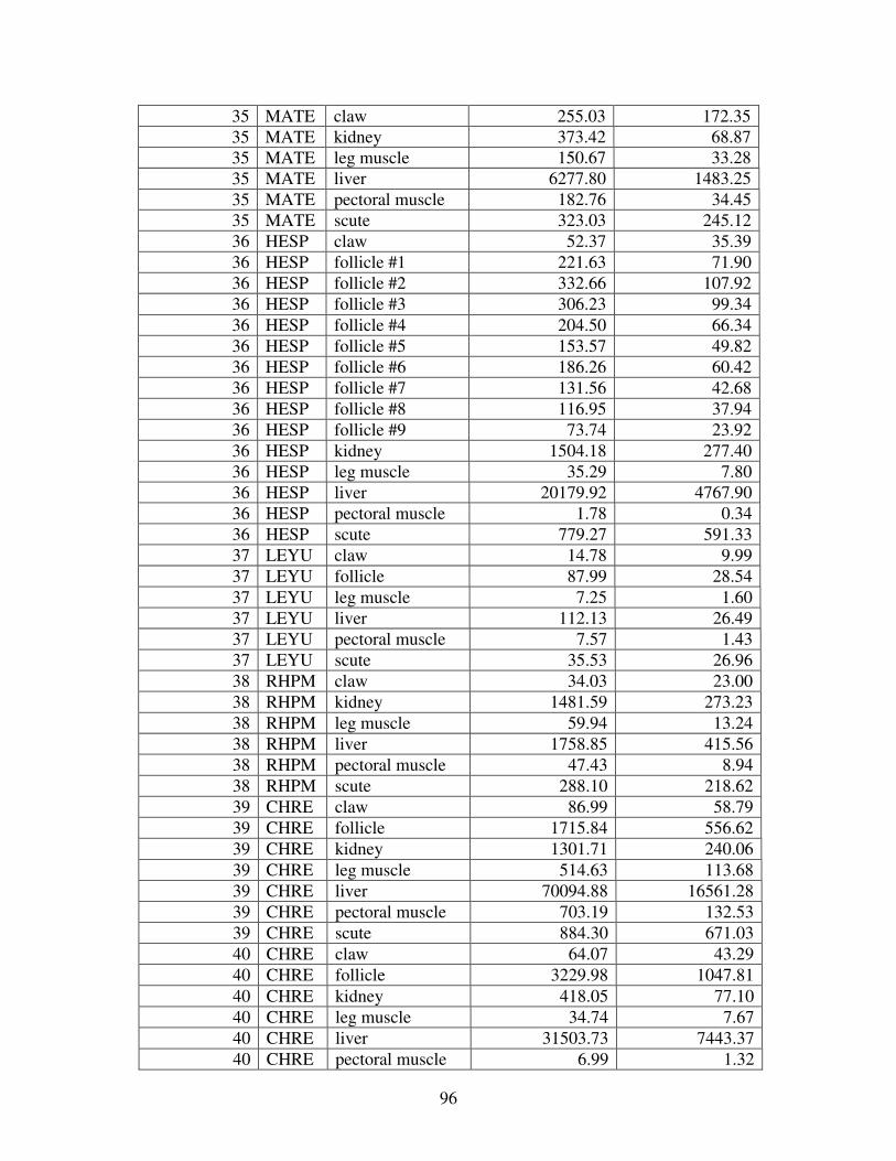
96
35 MATE claw 255.03 172.35
35 MATE kidney 373.42 68.87
35 MATE leg muscle 150.67 33.28
35 MATE liver 6277.80 1483.25
35 MATE pectoral muscle 182.76 34.45
35 MATE scute 323.03 245.12
36 HESP claw 52.37 35.39
36 HESP follicle #1 221.63 71.90
36 HESP follicle #2 332.66 107.92
36 HESP follicle #3 306.23 99.34
36 HESP follicle #4 204.50 66.34
36 HESP follicle #5 153.57 49.82
36 HESP follicle #6 186.26 60.42
36 HESP follicle #7 131.56 42.68
36 HESP follicle #8 116.95 37.94
36 HESP follicle #9 73.74 23.92
36 HESP kidney 1504.18 277.40
36 HESP leg muscle 35.29 7.80
36 HESP liver 20179.92 4767.90
36 HESP pectoral muscle 1.78 0.34
36 HESP scute 779.27 591.33
37 LEYU claw 14.78 9.99
37 LEYU follicle 87.99 28.54
37 LEYU leg muscle 7.25 1.60
37 LEYU liver 112.13 26.49
37 LEYU pectoral muscle 7.57 1.43
37 LEYU scute 35.53 26.96
38 RHPM claw 34.03 23.00
38 RHPM kidney 1481.59 273.23
38 RHPM leg muscle 59.94 13.24
38 RHPM liver 1758.85 415.56
38 RHPM pectoral muscle 47.43 8.94
38 RHPM scute 288.10 218.62
39 CHRE claw 86.99 58.79
39 CHRE follicle 1715.84 556.62
39 CHRE kidney 1301.71 240.06
39 CHRE leg muscle 514.63 113.68
39 CHRE liver 70094.88 16561.28
39 CHRE pectoral muscle 703.19 132.53
39 CHRE scute 884.30 671.03
40 CHRE claw 64.07 43.29
40 CHRE follicle 3229.98 1047.81
40 CHRE kidney 418.05 77.10
40 CHRE leg muscle 34.74 7.67
40 CHRE liver 31503.73 7443.37
40 CHRE pectoral muscle 6.99 1.32
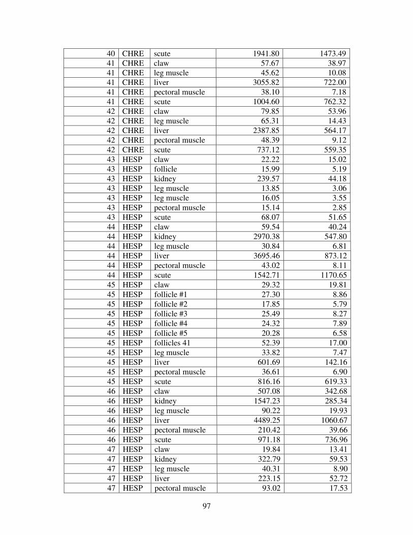
97
40 CHRE scute 1941.80 1473.49
41 CHRE claw 57.67 38.97
41 CHRE leg muscle 45.62 10.08
41 CHRE liver 3055.82 722.00
41 CHRE pectoral muscle 38.10 7.18
41 CHRE scute 1004.60 762.32
42 CHRE claw 79.85 53.96
42 CHRE leg muscle 65.31 14.43
42 CHRE liver 2387.85 564.17
42 CHRE pectoral muscle 48.39 9.12
42 CHRE scute 737.12 559.35
43 HESP claw 22.22 15.02
43 HESP follicle 15.99 5.19
43 HESP kidney 239.57 44.18
43 HESP leg muscle 13.85 3.06
43 HESP leg muscle 16.05 3.55
43 HESP pectoral muscle 15.14 2.85
43 HESP scute 68.07 51.65
44 HESP claw 59.54 40.24
44 HESP kidney 2970.38 547.80
44 HESP leg muscle 30.84 6.81
44 HESP liver 3695.46 873.12
44 HESP pectoral muscle 43.02 8.11
44 HESP scute 1542.71 1170.65
45 HESP claw 29.32 19.81
45 HESP follicle #1 27.30 8.86
45 HESP follicle #2 17.85 5.79
45 HESP follicle #3 25.49 8.27
45 HESP follicle #4 24.32 7.89
45 HESP follicle #5 20.28 6.58
45 HESP follicles 41 52.39 17.00
45 HESP leg muscle 33.82 7.47
45 HESP liver 601.69 142.16
45 HESP pectoral muscle 36.61 6.90
45 HESP scute 816.16 619.33
46 HESP claw 507.08 342.68
46 HESP kidney 1547.23 285.34
46 HESP leg muscle 90.22 19.93
46 HESP liver 4489.25 1060.67
46 HESP pectoral muscle 210.42 39.66
46 HESP scute 971.18 736.96
47 HESP claw 19.84 13.41
47 HESP kidney 322.79 59.53
47 HESP leg muscle 40.31 8.90
47 HESP liver 223.15 52.72
47 HESP pectoral muscle 93.02 17.53
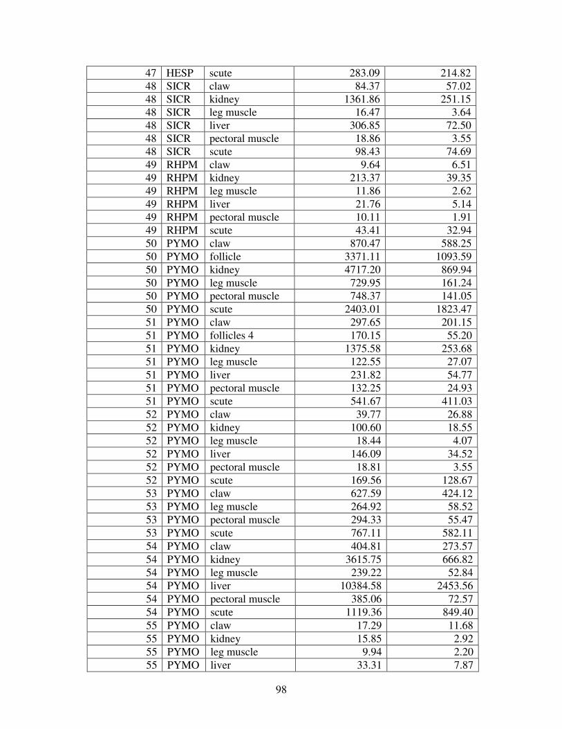
98
47 HESP scute 283.09 214.82
48 SICR claw 84.37 57.02
48 SICR kidney 1361.86 251.15
48 SICR leg muscle 16.47 3.64
48 SICR liver 306.85 72.50
48 SICR pectoral muscle 18.86 3.55
48 SICR scute 98.43 74.69
49 RHPM claw 9.64 6.51
49 RHPM kidney 213.37 39.35
49 RHPM leg muscle 11.86 2.62
49 RHPM liver 21.76 5.14
49 RHPM pectoral muscle 10.11 1.91
49 RHPM scute 43.41 32.94
50 PYMO claw 870.47 588.25
50 PYMO follicle 3371.11 1093.59
50 PYMO kidney 4717.20 869.94
50 PYMO leg muscle 729.95 161.24
50 PYMO pectoral muscle 748.37 141.05
50 PYMO scute 2403.01 1823.47
51 PYMO claw 297.65 201.15
51 PYMO follicles 4 170.15 55.20
51 PYMO kidney 1375.58 253.68
51 PYMO leg muscle 122.55 27.07
51 PYMO liver 231.82 54.77
51 PYMO pectoral muscle 132.25 24.93
51 PYMO scute 541.67 411.03
52 PYMO claw 39.77 26.88
52 PYMO kidney 100.60 18.55
52 PYMO leg muscle 18.44 4.07
52 PYMO liver 146.09 34.52
52 PYMO pectoral muscle 18.81 3.55
52 PYMO scute 169.56 128.67
53 PYMO claw 627.59 424.12
53 PYMO leg muscle 264.92 58.52
53 PYMO pectoral muscle 294.33 55.47
53 PYMO scute 767.11 582.11
54 PYMO claw 404.81 273.57
54 PYMO kidney 3615.75 666.82
54 PYMO leg muscle 239.22 52.84
54 PYMO liver 10384.58 2453.56
54 PYMO pectoral muscle 385.06 72.57
54 PYMO scute 1119.36 849.40
55 PYMO claw 17.29 11.68
55 PYMO kidney 15.85 2.92
55 PYMO leg muscle 9.94 2.20
55 PYMO liver 33.31 7.87
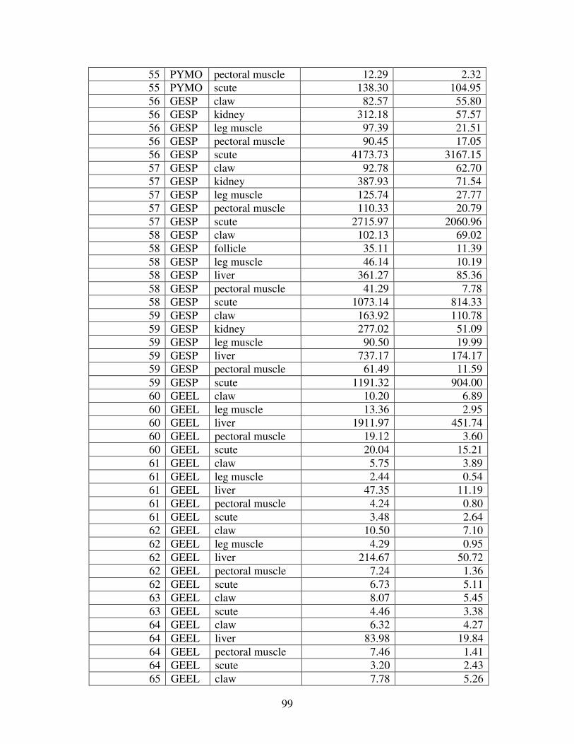
99
55 PYMO pectoral muscle 12.29 2.32
55 PYMO scute 138.30 104.95
56 GESP claw 82.57 55.80
56 GESP kidney 312.18 57.57
56 GESP leg muscle 97.39 21.51
56 GESP pectoral muscle 90.45 17.05
56 GESP scute 4173.73 3167.15
57 GESP claw 92.78 62.70
57 GESP kidney 387.93 71.54
57 GESP leg muscle 125.74 27.77
57 GESP pectoral muscle 110.33 20.79
57 GESP scute 2715.97 2060.96
58 GESP claw 102.13 69.02
58 GESP follicle 35.11 11.39
58 GESP leg muscle 46.14 10.19
58 GESP liver 361.27 85.36
58 GESP pectoral muscle 41.29 7.78
58 GESP scute 1073.14 814.33
59 GESP claw 163.92 110.78
59 GESP kidney 277.02 51.09
59 GESP leg muscle 90.50 19.99
59 GESP liver 737.17 174.17
59 GESP pectoral muscle 61.49 11.59
59 GESP scute 1191.32 904.00
60 GEEL claw 10.20 6.89
60 GEEL leg muscle 13.36 2.95
60 GEEL liver 1911.97 451.74
60 GEEL pectoral muscle 19.12 3.60
60 GEEL scute 20.04 15.21
61 GEEL claw 5.75 3.89
61 GEEL leg muscle 2.44 0.54
61 GEEL liver 47.35 11.19
61 GEEL pectoral muscle 4.24 0.80
61 GEEL scute 3.48 2.64
62 GEEL claw 10.50 7.10
62 GEEL leg muscle 4.29 0.95
62 GEEL liver 214.67 50.72
62 GEEL pectoral muscle 7.24 1.36
62 GEEL scute 6.73 5.11
63 GEEL claw 8.07 5.45
63 GEEL scute 4.46 3.38
64 GEEL claw 6.32 4.27
64 GEEL liver 83.98 19.84
64 GEEL pectoral muscle 7.46 1.41
64 GEEL scute 3.20 2.43
65 GEEL claw 7.78 5.26
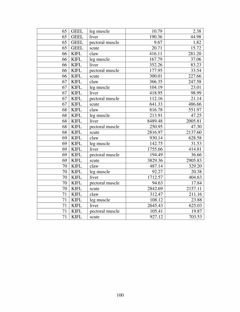
100
65 GEEL leg muscle 10.79 2.38
65 GEEL liver 190.36 44.98
65 GEEL pectoral muscle 9.67 1.82
65 GEEL scute 20.71 15.72
66 KIFL claw 416.11 281.20
66 KIFL leg muscle 167.79 37.06
66 KIFL liver 352.26 83.23
66 KIFL pectoral muscle 177.95 33.54
66 KIFL scute 300.01 227.66
67 KIFL claw 366.35 247.58
67 KIFL leg muscle 104.19 23.01
67 KIFL liver 418.95 98.99
67 KIFL pectoral muscle 112.16 21.14
67 KIFL scute 641.33 486.66
68 KIFL claw 816.78 551.97
68 KIFL leg muscle 213.91 47.25
68 KIFL liver 8489.48 2005.81
68 KIFL pectoral muscle 250.95 47.30
68 KIFL scute 2816.97 2137.60
69 KIFL claw 930.14 628.58
69 KIFL leg muscle 142.75 31.53
69 KIFL liver 1755.66 414.81
69 KIFL pectoral muscle 194.49 36.66
69 KIFL scute 3829.36 2905.83
70 KIFL claw 487.14 329.20
70 KIFL leg muscle 92.27 20.38
70 KIFL liver 1712.57 404.63
70 KIFL pectoral muscle 94.63 17.84
70 KIFL scute 2842.69 2157.11
71 KIFL claw 312.47 211.16
71 KIFL leg muscle 108.12 23.88
71 KIFL liver 2645.43 625.03
71 KIFL pectoral muscle 105.41 19.87
71 KIFL scute 927.12 703.53
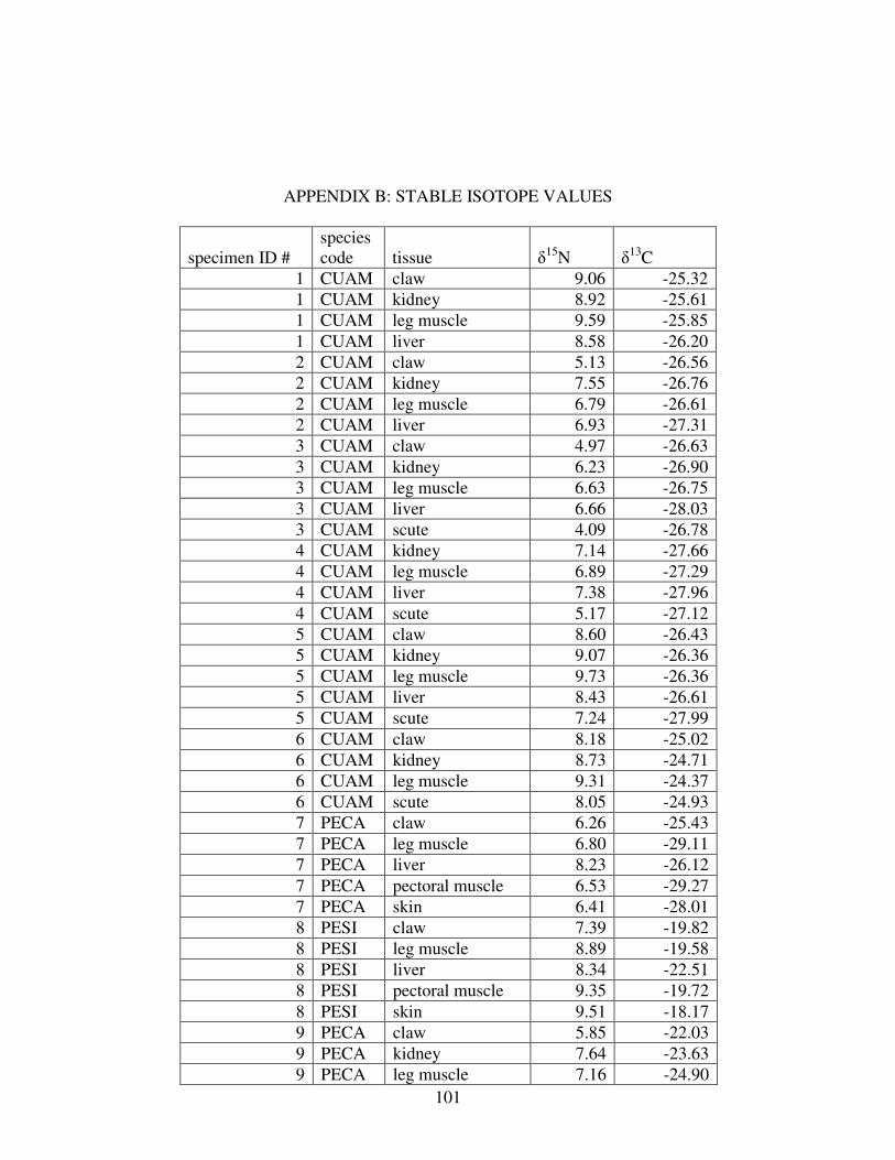
101
APPENDIX B: STABLE ISOTOPE VALUES
specimen ID # species code tissue δ
15N δ13C
1 CUAM claw 9.06 -25.32
1 CUAM kidney 8.92 -25.61
1 CUAM leg muscle 9.59 -25.85
1 CUAM liver 8.58 -26.20
2 CUAM claw 5.13 -26.56
2 CUAM kidney 7.55 -26.76
2 CUAM leg muscle 6.79 -26.61
2 CUAM liver 6.93 -27.31
3 CUAM claw 4.97 -26.63
3 CUAM kidney 6.23 -26.90
3 CUAM leg muscle 6.63 -26.75
3 CUAM liver 6.66 -28.03
3 CUAM scute 4.09 -26.78
4 CUAM kidney 7.14 -27.66
4 CUAM leg muscle 6.89 -27.29
4 CUAM liver 7.38 -27.96
4 CUAM scute 5.17 -27.12
5 CUAM claw 8.60 -26.43
5 CUAM kidney 9.07 -26.36
5 CUAM leg muscle 9.73 -26.36
5 CUAM liver 8.43 -26.61
5 CUAM scute 7.24 -27.99
6 CUAM claw 8.18 -25.02
6 CUAM kidney 8.73 -24.71
6 CUAM leg muscle 9.31 -24.37
6 CUAM scute 8.05 -24.93
7 PECA claw 6.26 -25.43
7 PECA leg muscle 6.80 -29.11
7 PECA liver 8.23 -26.12
7 PECA pectoral muscle 6.53 -29.27
7 PECA skin 6.41 -28.01
8 PESI claw 7.39 -19.82
8 PESI leg muscle 8.89 -19.58
8 PESI liver 8.34 -22.51
8 PESI pectoral muscle 9.35 -19.72
8 PESI skin 9.51 -18.17
9 PECA claw 5.85 -22.03
9 PECA kidney 7.64 -23.63
9 PECA leg muscle 7.16 -24.90
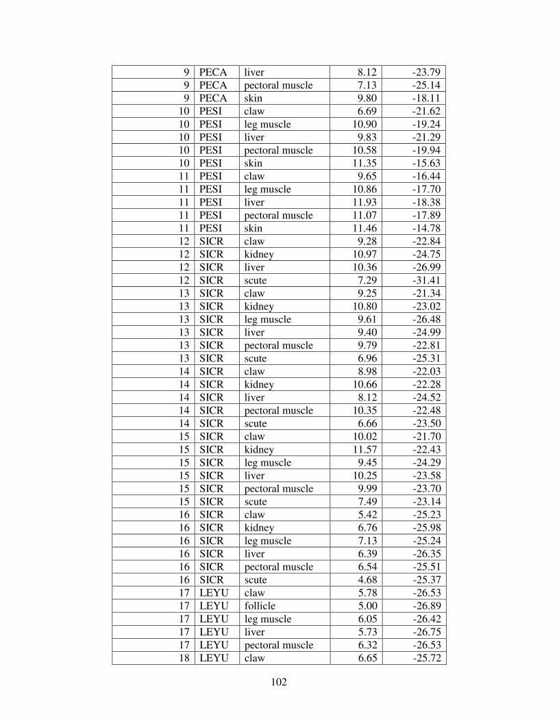
102
9 PECA liver 8.12 -23.79
9 PECA pectoral muscle 7.13 -25.14
9 PECA skin 9.80 -18.11
10 PESI claw 6.69 -21.62
10 PESI leg muscle 10.90 -19.24
10 PESI liver 9.83 -21.29
10 PESI pectoral muscle 10.58 -19.94
10 PESI skin 11.35 -15.63
11 PESI claw 9.65 -16.44
11 PESI leg muscle 10.86 -17.70
11 PESI liver 11.93 -18.38
11 PESI pectoral muscle 11.07 -17.89
11 PESI skin 11.46 -14.78
12 SICR claw 9.28 -22.84
12 SICR kidney 10.97 -24.75
12 SICR liver 10.36 -26.99
12 SICR scute 7.29 -31.41
13 SICR claw 9.25 -21.34
13 SICR kidney 10.80 -23.02
13 SICR leg muscle 9.61 -26.48
13 SICR liver 9.40 -24.99
13 SICR pectoral muscle 9.79 -22.81
13 SICR scute 6.96 -25.31
14 SICR claw 8.98 -22.03
14 SICR kidney 10.66 -22.28
14 SICR liver 8.12 -24.52
14 SICR pectoral muscle 10.35 -22.48
14 SICR scute 6.66 -23.50
15 SICR claw 10.02 -21.70
15 SICR kidney 11.57 -22.43
15 SICR leg muscle 9.45 -24.29
15 SICR liver 10.25 -23.58
15 SICR pectoral muscle 9.99 -23.70
15 SICR scute 7.49 -23.14
16 SICR claw 5.42 -25.23
16 SICR kidney 6.76 -25.98
16 SICR leg muscle 7.13 -25.24
16 SICR liver 6.39 -26.35
16 SICR pectoral muscle 6.54 -25.51
16 SICR scute 4.68 -25.37
17 LEYU claw 5.78 -26.53
17 LEYU follicle 5.00 -26.89
17 LEYU leg muscle 6.05 -26.42
17 LEYU liver 5.73 -26.75
17 LEYU pectoral muscle 6.32 -26.53
18 LEYU claw 6.65 -25.72
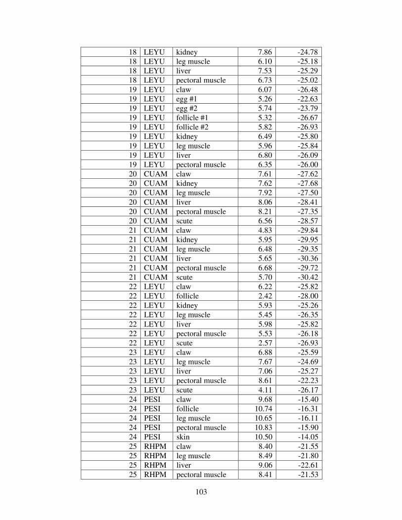
103
18 LEYU kidney 7.86 -24.78
18 LEYU leg muscle 6.10 -25.18
18 LEYU liver 7.53 -25.29
18 LEYU pectoral muscle 6.73 -25.02
19 LEYU claw 6.07 -26.48
19 LEYU egg #1 5.26 -22.63
19 LEYU egg #2 5.74 -23.79
19 LEYU follicle #1 5.32 -26.67
19 LEYU follicle #2 5.82 -26.93
19 LEYU kidney 6.49 -25.80
19 LEYU leg muscle 5.96 -25.84
19 LEYU liver 6.80 -26.09
19 LEYU pectoral muscle 6.35 -26.00
20 CUAM claw 7.61 -27.62
20 CUAM kidney 7.62 -27.68
20 CUAM leg muscle 7.92 -27.50
20 CUAM liver 8.06 -28.41
20 CUAM pectoral muscle 8.21 -27.35
20 CUAM scute 6.56 -28.57
21 CUAM claw 4.83 -29.84
21 CUAM kidney 5.95 -29.95
21 CUAM leg muscle 6.48 -29.35
21 CUAM liver 5.65 -30.36
21 CUAM pectoral muscle 6.68 -29.72
21 CUAM scute 5.70 -30.42
22 LEYU claw 6.22 -25.82
22 LEYU follicle 2.42 -28.00
22 LEYU kidney 5.93 -25.26
22 LEYU leg muscle 5.45 -26.35
22 LEYU liver 5.98 -25.82
22 LEYU pectoral muscle 5.53 -26.18
22 LEYU scute 2.57 -26.93
23 LEYU claw 6.88 -25.59
23 LEYU leg muscle 7.67 -24.69
23 LEYU liver 7.06 -25.27
23 LEYU pectoral muscle 8.61 -22.23
23 LEYU scute 4.11 -26.17
24 PESI claw 9.68 -15.40
24 PESI follicle 10.74 -16.31
24 PESI leg muscle 10.65 -16.11
24 PESI pectoral muscle 10.83 -15.90
24 PESI skin 10.50 -14.05
25 RHPM claw 8.40 -21.55
25 RHPM leg muscle 8.49 -21.80
25 RHPM liver 9.06 -22.61
25 RHPM pectoral muscle 8.41 -21.53
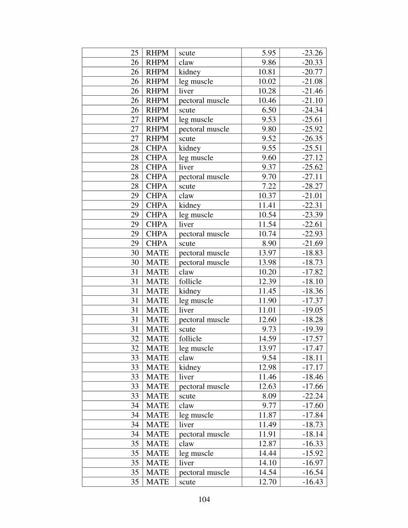
104
25 RHPM scute 5.95 -23.26
26 RHPM claw 9.86 -20.33
26 RHPM kidney 10.81 -20.77
26 RHPM leg muscle 10.02 -21.08
26 RHPM liver 10.28 -21.46
26 RHPM pectoral muscle 10.46 -21.10
26 RHPM scute 6.50 -24.34
27 RHPM leg muscle 9.53 -25.61
27 RHPM pectoral muscle 9.80 -25.92
27 RHPM scute 9.52 -26.35
28 CHPA kidney 9.55 -25.51
28 CHPA leg muscle 9.60 -27.12
28 CHPA liver 9.37 -25.62
28 CHPA pectoral muscle 9.70 -27.11
28 CHPA scute 7.22 -28.27
29 CHPA claw 10.37 -21.01
29 CHPA kidney 11.41 -22.31
29 CHPA leg muscle 10.54 -23.39
29 CHPA liver 11.54 -22.61
29 CHPA pectoral muscle 10.74 -22.93
29 CHPA scute 8.90 -21.69
30 MATE pectoral muscle 13.97 -18.83
30 MATE pectoral muscle 13.98 -18.73
31 MATE claw 10.20 -17.82
31 MATE follicle 12.39 -18.10
31 MATE kidney 11.45 -18.36
31 MATE leg muscle 11.90 -17.37
31 MATE liver 11.01 -19.05
31 MATE pectoral muscle 12.60 -18.28
31 MATE scute 9.73 -19.39
32 MATE follicle 14.59 -17.57
32 MATE leg muscle 13.97 -17.47
33 MATE claw 9.54 -18.11
33 MATE kidney 12.98 -17.17
33 MATE liver 11.46 -18.46
33 MATE pectoral muscle 12.63 -17.66
33 MATE scute 8.09 -22.24
34 MATE claw 9.77 -17.60
34 MATE leg muscle 11.87 -17.84
34 MATE liver 11.49 -18.73
34 MATE pectoral muscle 11.91 -18.14
35 MATE claw 12.87 -16.33
35 MATE leg muscle 14.44 -15.92
35 MATE liver 14.10 -16.97
35 MATE pectoral muscle 14.54 -16.54
35 MATE scute 12.70 -16.43
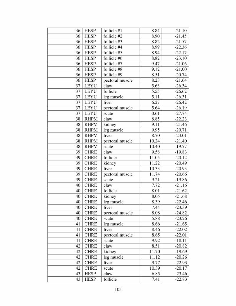
105
36 HESP follicle #1 8.84 -21.10
36 HESP follicle #2 8.90 -21.45
36 HESP follicle #3 8.82 -21.57
36 HESP follicle #4 8.99 -22.36
36 HESP follicle #5 8.94 -22.17
36 HESP follicle #6 8.82 -23.10
36 HESP follicle #7 9.47 -21.06
36 HESP follicle #8 9.12 -21.00
36 HESP follicle #9 8.51 -20.74
36 HESP pectoral muscle 8.23 -21.64
37 LEYU claw 5.63 -26.34
37 LEYU follicle 5.55 -26.62
37 LEYU leg muscle 5.11 -26.31
37 LEYU liver 6.27 -26.42
37 LEYU pectoral muscle 5.64 -26.19
37 LEYU scute 0.61 -27.74
38 RHPM claw 8.85 -22.23
38 RHPM kidney 9.11 -21.46
38 RHPM leg muscle 9.95 -20.71
38 RHPM liver 8.70 -23.01
38 RHPM pectoral muscle 10.24 -21.40
38 RHPM scute 10.40 -19.77
39 CHRE claw 9.58 -19.83
39 CHRE follicle 11.05 -20.12
39 CHRE kidney 11.22 -20.49
39 CHRE liver 10.33 -20.93
39 CHRE pectoral muscle 11.74 -20.66
39 CHRE scute 9.21 -19.86
40 CHRE claw 7.72 -21.16
40 CHRE follicle 8.01 -21.62
40 CHRE kidney 8.05 -21.68
40 CHRE leg muscle 8.39 -22.46
40 CHRE liver 7.44 -23.39
40 CHRE pectoral muscle 8.08 -24.82
40 CHRE scute 5.88 -23.26
41 CHRE leg muscle 8.66 -21.65
41 CHRE liver 8.46 -22.02
41 CHRE pectoral muscle 8.65 -22.01
41 CHRE scute 9.92 -18.11
42 CHRE claw 8.51 -20.82
42 CHRE kidney 11.70 -19.69
42 CHRE leg muscle 11.12 -20.26
42 CHRE liver 9.77 -22.93
42 CHRE scute 10.39 -20.17
43 HESP claw 6.85 -23.46
43 HESP follicle 7.41 -22.83
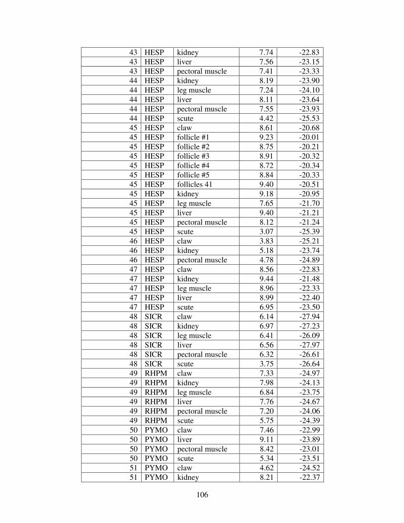
106
43 HESP kidney 7.74 -22.83
43 HESP liver 7.56 -23.15
43 HESP pectoral muscle 7.41 -23.33
44 HESP kidney 8.19 -23.90
44 HESP leg muscle 7.24 -24.10
44 HESP liver 8.11 -23.64
44 HESP pectoral muscle 7.55 -23.93
44 HESP scute 4.42 -25.53
45 HESP claw 8.61 -20.68
45 HESP follicle #1 9.23 -20.01
45 HESP follicle #2 8.75 -20.21
45 HESP follicle #3 8.91 -20.32
45 HESP follicle #4 8.72 -20.34
45 HESP follicle #5 8.84 -20.33
45 HESP follicles 41 9.40 -20.51
45 HESP kidney 9.18 -20.95
45 HESP leg muscle 7.65 -21.70
45 HESP liver 9.40 -21.21
45 HESP pectoral muscle 8.12 -21.24
45 HESP scute 3.07 -25.39
46 HESP claw 3.83 -25.21
46 HESP kidney 5.18 -23.74
46 HESP pectoral muscle 4.78 -24.89
47 HESP claw 8.56 -22.83
47 HESP kidney 9.44 -21.48
47 HESP leg muscle 8.96 -22.33
47 HESP liver 8.99 -22.40
47 HESP scute 6.95 -23.50
48 SICR claw 6.14 -27.94
48 SICR kidney 6.97 -27.23
48 SICR leg muscle 6.41 -26.09
48 SICR liver 6.56 -27.97
48 SICR pectoral muscle 6.32 -26.61
48 SICR scute 3.75 -26.64
49 RHPM claw 7.33 -24.97
49 RHPM kidney 7.98 -24.13
49 RHPM leg muscle 6.84 -23.75
49 RHPM liver 7.76 -24.67
49 RHPM pectoral muscle 7.20 -24.06
49 RHPM scute 5.75 -24.39
50 PYMO claw 7.46 -22.99
50 PYMO liver 9.11 -23.89
50 PYMO pectoral muscle 8.42 -23.01
50 PYMO scute 5.34 -23.51
51 PYMO claw 4.62 -24.52
51 PYMO kidney 8.21 -22.37
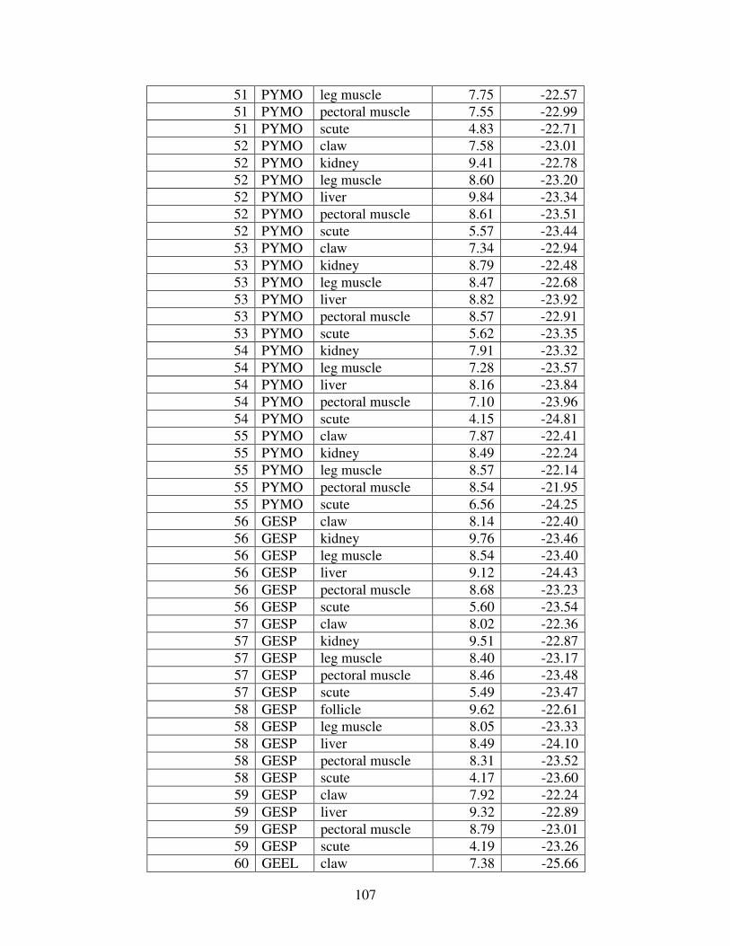
107
51 PYMO leg muscle 7.75 -22.57
51 PYMO pectoral muscle 7.55 -22.99
51 PYMO scute 4.83 -22.71
52 PYMO claw 7.58 -23.01
52 PYMO kidney 9.41 -22.78
52 PYMO leg muscle 8.60 -23.20
52 PYMO liver 9.84 -23.34
52 PYMO pectoral muscle 8.61 -23.51
52 PYMO scute 5.57 -23.44
53 PYMO claw 7.34 -22.94
53 PYMO kidney 8.79 -22.48
53 PYMO leg muscle 8.47 -22.68
53 PYMO liver 8.82 -23.92
53 PYMO pectoral muscle 8.57 -22.91
53 PYMO scute 5.62 -23.35
54 PYMO kidney 7.91 -23.32
54 PYMO leg muscle 7.28 -23.57
54 PYMO liver 8.16 -23.84
54 PYMO pectoral muscle 7.10 -23.96
54 PYMO scute 4.15 -24.81
55 PYMO claw 7.87 -22.41
55 PYMO kidney 8.49 -22.24
55 PYMO leg muscle 8.57 -22.14
55 PYMO pectoral muscle 8.54 -21.95
55 PYMO scute 6.56 -24.25
56 GESP claw 8.14 -22.40
56 GESP kidney 9.76 -23.46
56 GESP leg muscle 8.54 -23.40
56 GESP liver 9.12 -24.43
56 GESP pectoral muscle 8.68 -23.23
56 GESP scute 5.60 -23.54
57 GESP claw 8.02 -22.36
57 GESP kidney 9.51 -22.87
57 GESP leg muscle 8.40 -23.17
57 GESP pectoral muscle 8.46 -23.48
57 GESP scute 5.49 -23.47
58 GESP follicle 9.62 -22.61
58 GESP leg muscle 8.05 -23.33
58 GESP liver 8.49 -24.10
58 GESP pectoral muscle 8.31 -23.52
58 GESP scute 4.17 -23.60
59 GESP claw 7.92 -22.24
59 GESP liver 9.32 -22.89
59 GESP pectoral muscle 8.79 -23.01
59 GESP scute 4.19 -23.26
60 GEEL claw 7.38 -25.66
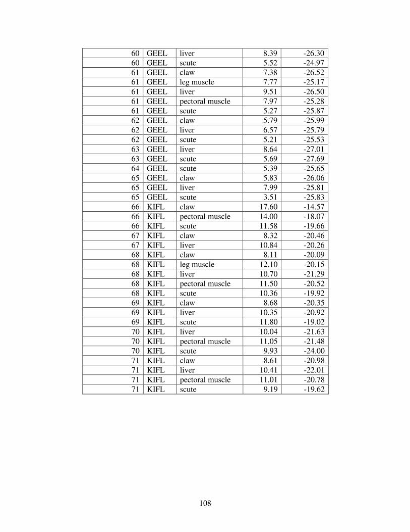
108
60 GEEL liver 8.39 -26.30
60 GEEL scute 5.52 -24.97
61 GEEL claw 7.38 -26.52
61 GEEL leg muscle 7.77 -25.17
61 GEEL liver 9.51 -26.50
61 GEEL pectoral muscle 7.97 -25.28
61 GEEL scute 5.27 -25.87
62 GEEL claw 5.79 -25.99
62 GEEL liver 6.57 -25.79
62 GEEL scute 5.21 -25.53
63 GEEL liver 8.64 -27.01
63 GEEL scute 5.69 -27.69
64 GEEL scute 5.39 -25.65
65 GEEL claw 5.83 -26.06
65 GEEL liver 7.99 -25.81
65 GEEL scute 3.51 -25.83
66 KIFL claw 17.60 -14.57
66 KIFL pectoral muscle 14.00 -18.07
66 KIFL scute 11.58 -19.66
67 KIFL claw 8.32 -20.46
67 KIFL liver 10.84 -20.26
68 KIFL claw 8.11 -20.09
68 KIFL leg muscle 12.10 -20.15
68 KIFL liver 10.70 -21.29
68 KIFL pectoral muscle 11.50 -20.52
68 KIFL scute 10.36 -19.92
69 KIFL claw 8.68 -20.35
69 KIFL liver 10.35 -20.92
69 KIFL scute 11.80 -19.02
70 KIFL liver 10.04 -21.63
70 KIFL pectoral muscle 11.05 -21.48
70 KIFL scute 9.93 -24.00
71 KIFL claw 8.61 -20.98
71 KIFL liver 10.41 -22.01
71 KIFL pectoral muscle 11.01 -20.78
71 KIFL scute 9.19 -19.62
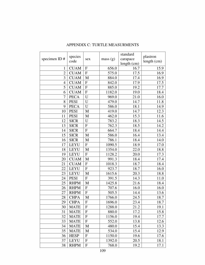
109
APPENDIX C: TURTLE MEASURMENTS
specimen ID # species code
sex mass (g) standard carapace length (cm)
plastron length (cm)
1 CUAM F 656.0 16.7 15.9
2 CUAM F 575.0 17.5 16.9
3 CUAM M 884.0 17.4 16.9
4 CUAM F 842.0 17.9 17.5
5 CUAM F 885.0 19.2 17.7
6 CUAM F 1182.0 19.0 18.4
7 PECA U 969.0 21.0 16.0
8 PESI U 479.0 14.7 11.8
9 PECA U 586.0 18.1 14.9
10 PESI M 419.0 14.7 12.3
11 PESI M 462.0 15.3 11.6
12 SICR U 783.2 18.3 14.5
13 SICR F 762.3 18.5 14.2
14 SICR F 664.7 18.4 14.4
15 SICR M 586.0 16.4 13.4
16 SICR M 786.1 18.4 14.0
17 LEYU F 1090.5 18.9 17.0
18 LEYU M 1354.0 22.0 18.8
19 LEYU F 1128.2 20.0 17.3
20 CUAM M 991.3 18.4 17.4
21 CUAM F 1018.3 18.7 18.4
22 LEYU F 923.7 18.7 16.0
23 LEYU M 1615.6 20.3 18.8
24 PESI F 391.5 14.3 11.0
25 RHPM M 1425.8 21.6 18.4
26 RHPM F 707.6 16.0 16.0
27 RHPM F 505.5 14.4 13.6
28 CHPA M 1766.0 24.5 18.7
29 CHPA F 1696.0 23.4 18.7
30 MATE F 1288.0 21.2 19.1
31 MATE F 880.0 17.2 15.8
32 MATE F 1156.0 19.4 17.7
33 MATE F 552.0 13.8 12.6
34 MATE M 480.0 15.4 13.3
35 MATE M 534.0 15.4 12.9
36 HESP F 1150.0 19.6 17.6
37 LEYU F 1392.0 20.5 18.1
38 RHPM F 768.0 19.2 17.1
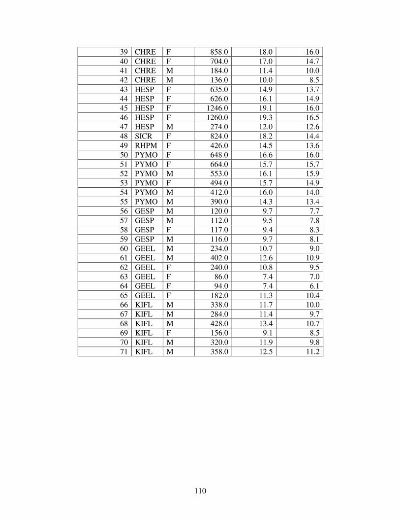
110
39 CHRE F 858.0 18.0 16.0
40 CHRE F 704.0 17.0 14.7
41 CHRE M 184.0 11.4 10.0
42 CHRE M 136.0 10.0 8.5
43 HESP F 635.0 14.9 13.7
44 HESP F 626.0 16.1 14.9
45 HESP F 1246.0 19.1 16.0
46 HESP F 1260.0 19.3 16.5
47 HESP M 274.0 12.0 12.6
48 SICR F 824.0 18.2 14.4
49 RHPM F 426.0 14.5 13.6
50 PYMO F 648.0 16.6 16.0
51 PYMO F 664.0 15.7 15.7
52 PYMO M 553.0 16.1 15.9
53 PYMO F 494.0 15.7 14.9
54 PYMO M 412.0 16.0 14.0
55 PYMO M 390.0 14.3 13.4
56 GESP M 120.0 9.7 7.7
57 GESP M 112.0 9.5 7.8
58 GESP F 117.0 9.4 8.3
59 GESP M 116.0 9.7 8.1
60 GEEL M 234.0 10.7 9.0
61 GEEL M 402.0 12.6 10.9
62 GEEL F 240.0 10.8 9.5
63 GEEL F 86.0 7.4 7.0
64 GEEL F 94.0 7.4 6.1
65 GEEL F 182.0 11.3 10.4
66 KIFL M 338.0 11.7 10.0
67 KIFL M 284.0 11.4 9.7
68 KIFL M 428.0 13.4 10.7
69 KIFL F 156.0 9.1 8.5
70 KIFL M 320.0 11.9 9.8
71 KIFL M 358.0 12.5 11.2