Embed Size (px)
Citation preview
NASA-ER-202579
MCR-96-1303, Issue 02
Contract Number: NAS8-40633
i/ k/ /" i ¸
/
f_ ._ x--,_.2._-
Membrane Transport Phenomena (MTP)
Semi-Annual
Technical Progress Report
May 1996 - November 1996
Principal hhvestigator, Program Manager:Larry W. Mason
Prepared By:Lockheed Martin Astronautics Company
Flight Systems DivisionP.O. Box 179
Denver, CO 80201
Prepared For:National Aeronautics and Space Administration
George C. Marshall Space Flight CenterMarshall Space Flight Center, AL 35812
LOCKHEED MA R TIN/__
https://ntrs.nasa.gov/search.jsp?R=19970001740 2018-06-14T18:52:30+00:00Z

Table of Contents
MTP EXPERIMENT DEVELOPMENT .......................................................... 1
MEMBRANE TO FLUID OPTICAL CELL SEAL DEVELOPMENT ....................... 1
VOLUMETRIC FLOW SENSOR (VFS) DEVELOPEMENT ................................. 5
HYDROSTATIC PRESSURE EXPERIMENTS ................................................. 6
MEMBRANE EVALUATION ACTIVITIES ..................................................... 8
MTA OSMOSIS EXPERIMENTS ................................................................ 10
Experimental Solutions .......................................................................... 11Experimental Data Acquisition .................................................................. 12Solute on Top (+lg) Experimental Results ......................................... : .......... 14Solute on Bottom (-lg) Experimental Results ................................................ 17
MTA FLUID MANIPULATION SYSTEMS (FMS) DEVELOPMENT ..................... 20
FMS SOFTWARE DEVELOPMENT ............................................................ 22
REFRACTOMETER IMAGE ANALYSIS SOFTWARE DEVELOPMENT ................ 24
MTA REFRACTOMETER CALIBRATION .................................................... 27
MTP ANALYTICAL MODEL DEVELOPMENT .............................................. 33
DC-9 MICROGRAVITY EXPERIMENT DEVELOPMENT .................................. 37
Fluid Manipulation System (FMS) Experiment ............................................... 37Refractometer Verification Experiment (RVE) ................................................ 37DC-9 Experiment Hardware Description ...................................................... 38
MICROSENSOR ARRAY DEVELOPMENT ................................................... 42
MICROSENSOR ARRAY INTERFACE ELECTRONICS DEVELOPMENT ............. 43

MTP Technical Report II 1
MTP EXPERIMENT DEVELOPMENT
The first generation instrument for the Membrane Transport Phenomena (MTP) experimentis complete, and is called the Membrane Transport Apparatus (MTA). The MTA is aprototype instrument that is designed to perform precision measurements on membranemediated transport phenomena. Several subsystems of the instrument have been developedin parallel over the last six months. These subsystems are all interrelated, and thedevelopment activity was shared among the various systems as the instrument matured.The subsystems include: the membrane to Fluid Optical Cell (FOC) seal, data acquisitioninterfaces and software, and refractometer calibration and image processing software.Additionally, the MTA Fluid Manipulation System (FMS) has evolved to provide automaticcontrol over filling and draining operations and the Volumetric Flow Sensors (VFS) have
been upgraded. A series of experiments using the MTA have been conducted to calibratethe sensors, establish instrument sensitivities, characterize membranes, and measure
osmosis. The subsystem development and experimental activities are detailed in followingsections.
MEMBRANE TO FLUID OPTICAL CELL SEAL DEVELOPMENT
The development of the seal between the membrane and the Fluid Optical Cells (FOC) hasbeen a high priority activity. This seal occurs at an interface in the instrument where threekey functions must be realized: (1) physical membrane support, (2) fluid sealing, and (3)unobscured optical transmission.
This fluid cell seal provides physical support for the membrane. The membrane is securedaround the perimeter, captivated by the fluid cell sealing surfaces and compressed betweenthe two fluid cells. The fluids exert a hydrostatic force on the membrane that changes asthe fluids move from one compartment to the other. The magnitude of the hydrostatic force(pressure head) is determined by the relative level of fluid within the two Volumetric FlowSensors (VFS). As these levels change relative to each other, the force exerted on themembrane also changes, and the membrane physically moves. The movement of themembrane is restrained by the seal, and it can pull free from the seal if enough hydrostatic
pressure is applied.
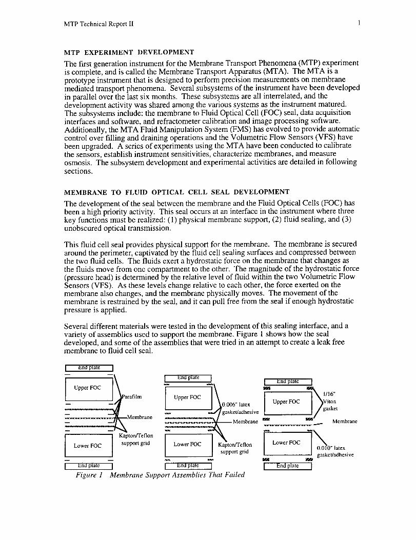
Several different materials were tested in the development of this sealing interface, and avariety of assemblies used to support the membrane. Figure 1 shows how the seal
developed, and some of the assemblies that were tried in an attempt to create a leak freemembrane to fluid cell seal.
I End plate
Upper FOC
m _J
_K_KXK_K_KXK_KXKXK}'
: ....................... ..3
I Lower FOC
D m
i end plate l
Figure 1
I ena plate [ I izna plate I
I/ as °t_Membrane -- _'J/gasket/adhesive ."
Kapton/Teflon _:__ Membrane
support grid Lower FOC Kapton/Teflon
support grid
[ e,noplate J
Membrane Support Assemblies That Failed
m Membrane
-[ End plate j
MTP Technical Report II 2
Parafilm, a waxy material that is commonly used in laboratories to seal glassware, wasinitially used to make sealing gaskets for the MTA. This proved not to be effective, eitheralone or in combination with membrane support grids. In another attempt, a sandwichassembly was created using altemating layers of Parafilm and Kapton with the membranein the middle. This configuration also proved not to be functional in terms of fluid leaks.
Latex rubber sheet material was used to fabricate gaskets of various thickness for themembrane to fluid cell seal. Initially, a 0.006" thick latex gasket was fabricated in the
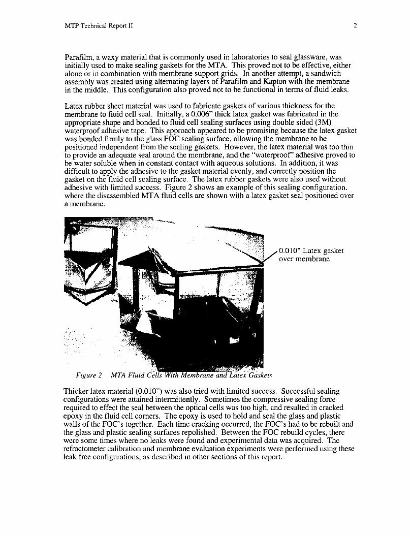
appropriate shape and bonded to fluid cell sealing surfaces using double sided (3M)waterproof adhesive tape. This approach appeared to be promising because the latex gasketwas bonded firmly to the glass FOC sealing surface, allowing the membrane to bepositioned independent from the sealing gaskets. However, the latex material was too thinto provide an adequate seal around the membrane, and the "waterproof" adhesive proved tobe water soluble when in constant contact with aqueous solutions. In addition, it wasdifficult to apply the adhesive to the gasket material evenly, and correctly position thegasket on the fluid cell sealing surface. The latex rubber gaskets were also used withoutadhesive with limited success. Figure 2 shows an example of this sealing configuration,where the disassembled MTA fluid cells are shown with a latex gasket seal positioned overa membrane.
10" Latex gasketover membrane
•;._ ....Figure 2 MTA Fluid Cells With Membrane and Latex Gaskets
Thicker latex material (0.010") was also tried with limited success. Successful sealingconfigurations were attained intermittently. Sometimes the compressive sealing force
required to effect the seal between the optical cells was too high, and resulted in crackedepoxy in the fluid cell comers. The epoxy is used to hold and seal the glass and plasticwalls of the FOC's together. Each time cracking occurred, the FOC's had to be rebuilt andthe glass and plastic sealing surfaces repolished. Between the FOC rebuild cycles, therewere some times where no leaks were found and experimental data was acquired. Therefractometer calibration and membrane evaluation experiments were performed using theseleak free configurations, as described in other sections of this report.
MTP Technical Report II 3
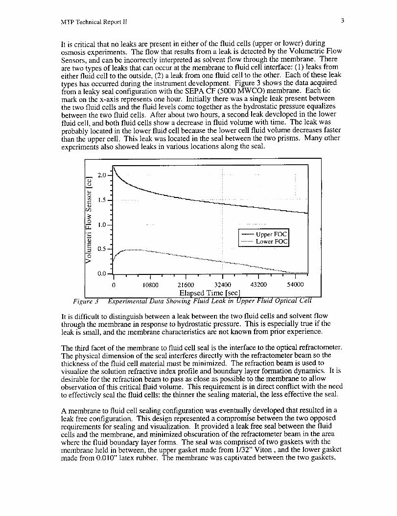
It is critical that no leaks are present in either of the fluid cells (upper or lower) duringosmosis experiments. The flow that results from a leak is detected by the Volumetric FlowSensors, and can be incorrectly interpreted as solvent flow through the membrane. Thereare two types of leaks that can occur at the membrane to fluid cell interface: (1) leaks fromeither fluid cell to the outside, (2) a leak from one fluid cell to the other. Each of these leak
types has occurred during the instrument development. Figure 3 shows the data acquiredfrom a leaky seal configuration with the SEPA CF (5000 MWCO) membrane. Each ticmark on the x-axis represents one hour. Initially there was a single leak present betweenthe two fluid cells and the fluid levels come together as the hydrostatic pressure equalizesbetween the two fluid cells. After about two hours, a second leak developed in the lowerfluid cell, and both fluid cells show a decrease in fluid volume with time. The leak was
probably located in the lower fluid cell because the lower cell fluid volume decreases fasterthan the upper cell. This leak was located in the seal between the two prisms. Many other
experiments also showed leaks in various locations along the seal.
e-,
:t3
©_Z
=_D
E
o>
Figure 3
2o11.5--4
1.0 --]
0.0_ ia !
0 10800
' I '
21600
Upper FOC [
......... Lower FOC[
"'"..-_..°...,..,...
'°-.--..,......
-°--4 ................
' I ' ' I ' ' I
32400 43200 54000
Elapsed Time [sec]Experimental Data Showing Fluid Leak in Upper Fluid Optical Cell
It is difficult to distinguish between a leak between the two fluid cells and solvent flowthrough the membrane in response to hydrostatic pressure. This is especially true if theleak is small, and the membrane characteristics are not known from prior experience.
The third facet of the membrane to fluid cell seal is the interface to the optical refractometer.
The physical dimension of the seal interferes directly with the refractometer beam so thethickness of the fluid cell material must be minimized. The refraction beam is used to
visualize the solution refractive index profile and boundary layer formation dynamics. It isdesirable for the refraction beam to pass as close as possible to the membrane to allowobservation of this critical fluid volume. This requirement is in direct conflict with the needto effectively seal the fluid cells: the thinner the sealing material, the less effective the seal.
A membrane to fluid cell sealing configuration was eventually developed that resulted in aleak free configuration. This design represented a compromise between the two opposedrequirements for sealing and visualization. It provided a leak free seal between the fluidcells and the membrane, and minimized obscuration of the refractometer beam in the area
where the fluid boundary layer forms The seal was comprised of two gaskets with themembrane held in between, the upper gasket made from 1/32" Viton, and the lower gasketmade from 0.010" latex rubber. The membrane was captivated between the two gaskets,
MTPTechnicalReportII 4
creatingasealbetweenthefluid cellsandthemembrane.ThethickerVitongasketprovidedthesealingcompliancefor themembraneto fluid cell interface,andthelowergasketwasverythin to allowvisualizationof therefractiveindexprofileon thelowersideof themembrane.TheViton gasketcompressedto about1mmthicknesswhenin theMTA, obscuringtherefractometerbeamonly on theuppersideof themembrane.Thelatexrubbergasketobscuredlessthan0.2mmof therefractometerbeam,allowingvisualizationof thelower sideof themembraneandboundarylayerformationdynamics.Theboundarylayerformsonly on thelowersideof themembrane,andthethickerViton gasketdidnotinterferewith therefractometeropticson thelowerside.
Thismembranesealconfigurationwasfunctional,butproveddifficult to maintain.Whenthemembraneandsealingcomponentswereassembled,themembranehadtobe trimmedandinstalledthroughtrial anderroruntil no leaksweredetected.Thephysicalsizeof themembranewascritical, it hadtocovera largeenoughportionof thefluid cell sealingsurfaceto becompressedby thefluid cells,andleaveenoughof thegasketmaterialexposedtotheedgesto createaseal.Additionally, therelativepositionsof thetwogaskets,themembrane,andtheopticalcell sealingsurfacesall hadtobealignedexactlytoeffect thesealwhentheentireassemblywasinstalledwithin thesupportframe. If anyofthesecomponentswasout of positionby even0.4mm, aleakresulted.Further,a largecompressivesealingforcewasrequiredto insurethatthesealinggasketscontactedeachotheraroundthemembraneperiphery.Onoccasion,thiscompressiveforceprovedto bedestructiveto theepoxysealsthatholdtheFOCopticalcomponentstogether.Whentheepoxybecamedetachedor cracked,theprismandsidewindowshadto becompletelydisassembled,re-epoxyed,andthesealingsurfacesre-polished.
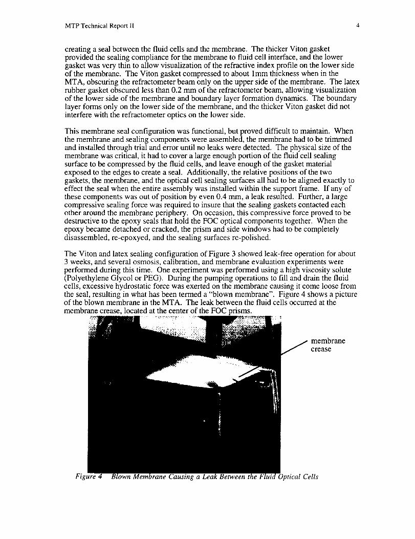
TheVitonandlatexsealingconfigurationof Figure3 showedleak-fleeoperationfor about3 weeks,andseveralosmosis,calibration,andmembraneevaluationexperimentswereperformedduringthis time. Oneexperimentwasperformedusingahighviscositysolute(PolyethyleneGlycolor PEG). During thepumpingoperationsto fill anddrainthefluidcells,excessivehydrostaticforcewasexertedon themembranecausingit comeloosefromtheseal,resultingin whathasbeentermeda"blown membrane".Figure4 showsapictureof theblownmembranein theMTA. Theleakbetweenthefluid cellsoccurredatthemembranecrease,locatedatthecenterof theFOC prisms.
membrane
crease
Figure 4 Blown Mem, _rane Causing a Leak Between the Optical Cells
MTP Technical Report II 5
The high pressure across the membrane was caused by a combination of the high viscositysolute, and malfunctioning valves. The valve malfunction is described in the FluidManipulation System section of this report. The blown membrane required that the MTAbe disassembled to replace the membrane. During this activity it was seen that the epoxyhad loosened in a corner of the lower FOC, at it was beginning to leak. This was
presumably caused by the high compressive force required to effect the seal. The fluid cellassembly had to be completely rebuilt and sealing surfaces re-polished. After rebuilding,the leak-free configuration was not attainable using these same sealing materials.
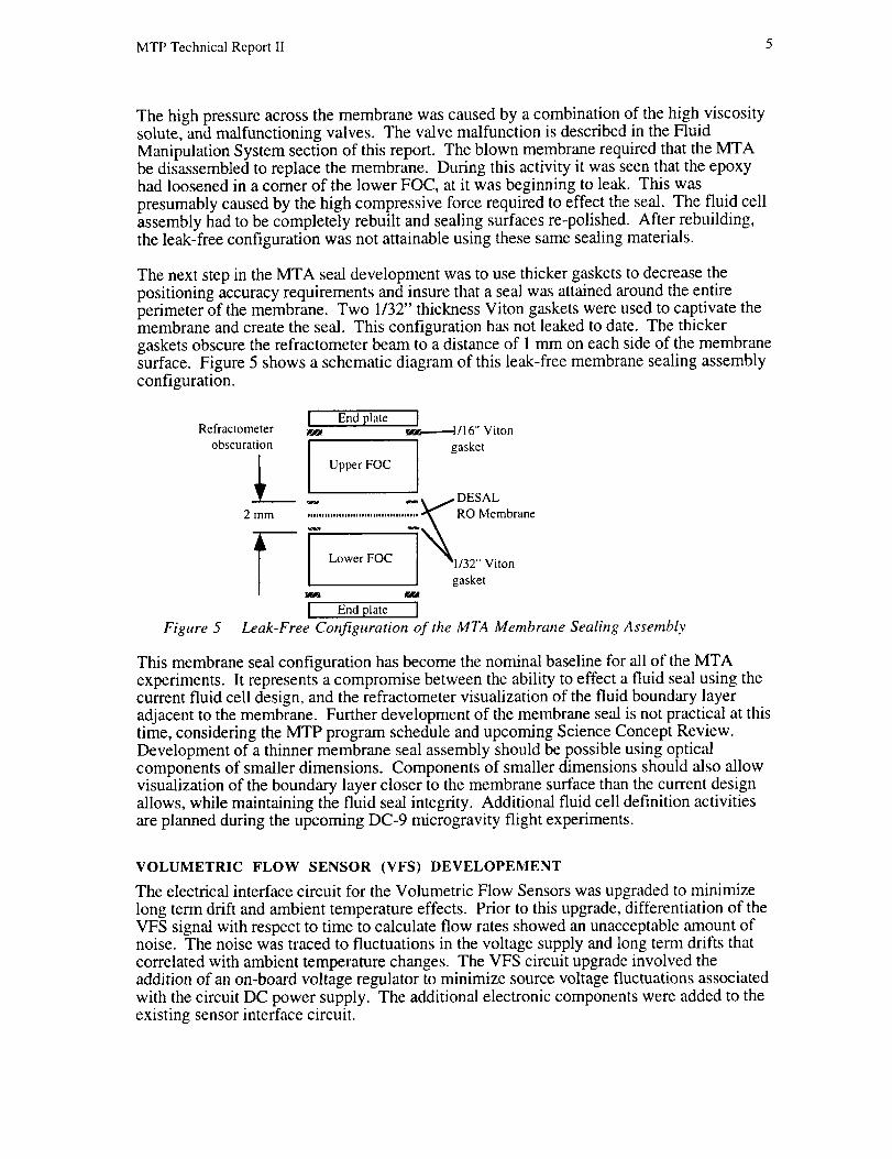
The next step in the MTA seal development was to use thicker gaskets to decrease thepositioning accuracy requirements and insure that a seal was attained around the entireperimeter of the membrane. Two 1/32" thickness Viton gaskets were used to captivate themembrane and create the seal. This configuration has not leaked to date. The thicker
gaskets obscure the refractometer beam to a distance of 1 mm on each side of the membranesurface. Figure 5 shows a schematic diagram of this leak-free membrane sealing assemblyconfiguration.
Refractometer
obscuration
l_2 mm
Figure 5
End plate [_------q /16" Viton
-- _I_._ DESAL
Lower FOC _1/32" Viton....i .................................. _ RO Membrane
_ _ gasket
[ End plate ]
Leak-Free Configuration of the MTA Membrane Sealing Assembly
This membrane seal configuration has become the nominal baseline for all of the MTA
experiments. It represents a compromise between the ability to effect a fluid seal using thecurrent fluid cell design, and the refractometer visualization of the fluid boundary layeradjacent to the membrane. Further development of the membrane seal is not practical at this
time, considering the MTP program schedule and upcoming Science Concept Review.Development of a thinner membrane seal assembly should be possible using opticalcomponents of smaller dimensions. Components of smaller dimensions should also allowvisualization of the boundary layer closer to the membrane surface than the current designallows, while maintaining the fluid seal integrity. Additional fluid cell definition activitiesare planned during the upcoming DC-9 microgravity flight experiments.
VOLUMETRIC FLOW SENSOR (VFS) DEVELOPEMENT
The electrical interface circuit for the Volumetric Flow Sensors was upgraded to minimize
long term drift and ambient temperature effects. Prior to this upgrade, differentiation of theVFS signal with respect to time to calculate flow rates showed an unacceptable amount ofnoise. The noise was traced to fluctuations in the voltage supply and long term drifts thatcorrelated with ambient temperature changes. The VFS circuit upgrade involved theaddition of an on-board voltage regulator to minimize source voltage fluctuations associatedwith the circuit DC power supply. The additional electronic components were added to theexisting sensor interface circuit.
MTP Technical Report II 6
The data acquisition software for the VFS system was also upgraded. The upgradedsoftware allows specification of the acquisition speed and resolution of the VFS data.Course resolution data can now be acquired at high speed for fluid manipulation
operations. The increased acquisition speed is useful during the closed loop pumpingoperations to minimize the time lag associated with data acquisition. Slower, highresolution data is acquired during the osmotic and hydrostatic flow experiments. Thesensor noise problem was further reduced by acquiring the sensor reading over a onesecond interval, and averaging the value. The time averaging increased the signal to noiseratio of the data, and dramatically lowered the scatter in the differentiated VFS data.
A calibration protocol was developed for the VFS. This protocol involves first calibratingthe peristaltic pumps using a mass balance to measure pumped volumes. The calibratedvolumes are then pumped into the VFS and the sensor outputs recorded. The solvent masscontained within the VFS can then be correlated to the sensor output signal using aregression analysis. The sensors were shown to be linear devices. Two coefficients aredefined that can be used to convert the voltage output to contained VFS solvent mass. BothVFS were re-calibrated with DI water for use in the osmosis and hydrostatic experiments.The calibration software for both the peristaltic pumps and the VFS were developed inconjunction with the MTA Fluid Manipulation System (FMS), described in another sectionof this report.
HYDROSTATIC PRESSURE EXPERIMENTS
During the membrane to fluid cell seal development, membranes of different types weretested in the MTA for sealing, deformation, and hydrostatic flow characteristics. Theseexperiments were conducted as the development of the MTA seal allowed, and were usedto characterize the seal assemblies and membranes. An experimental protocol and data
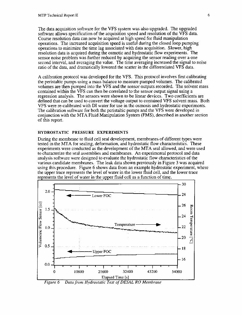
analysis software were designed to evaluate the hydrostatic flow characteristics of thevarious candidate membranes. The leak data shown previously in Figure 3 was acquiredusing this procedure. Figure 6 shows data from an example hydrostatic experiment, wherethe upper trace represents the level of water in the lower fluid cell, and the lower trace
represents the level of water in the upper fluid cell as a function of time.
t3°2.0 .----- ....Lower FOC 28
26O
_ 1.5 ............ .................. ....................iemperat u......................................... t24 3re. ""- 22 a10.-0
E - 20
•-_ :
> 0.5 ..................................................................................................: -18
_'_-.,, Upper FOCw
0.0-' ' I .... I ' ' I '
Figure 6
10800 21600 32400 43200
Elapsed Time [s]Data from Hydrostatic Test of DESAL RO Membrane
-16
!
54000
MTP Technical Report II 7
The hydrostatic experiments consist of first establishing a leak-free membrane sealingconfiguration, then applying a measured hydrostatic pressure across the membrane, andcollecting kinetic data for solvent flow through the membrane. The hydrostatic drivingforce in the MTA is defined by the difference in fluid level between the two fluid cells, eachfilled to a different level with deionized water. The two Volumetric Flow Sensors are
secured at the same height relative to the fluid cells, but are filled with fluid to differentlevels. When one VFS is full and the other almost empty, a maximum of about 4" of
pressure head is present across the membrane. The displacement of each membrane testedunder the influence of this pressure was observed and noted, and data collected for solvent
flow using the VFS. As the hydrostatic pressure caused water to flow through themembrane, the level in each of the volumetric flow sensors changed, and was recorded as afunction of time. The levels in the two Volumetric Flow Sensors come together as the
hydrostatic pressure across the membrane equalizes.
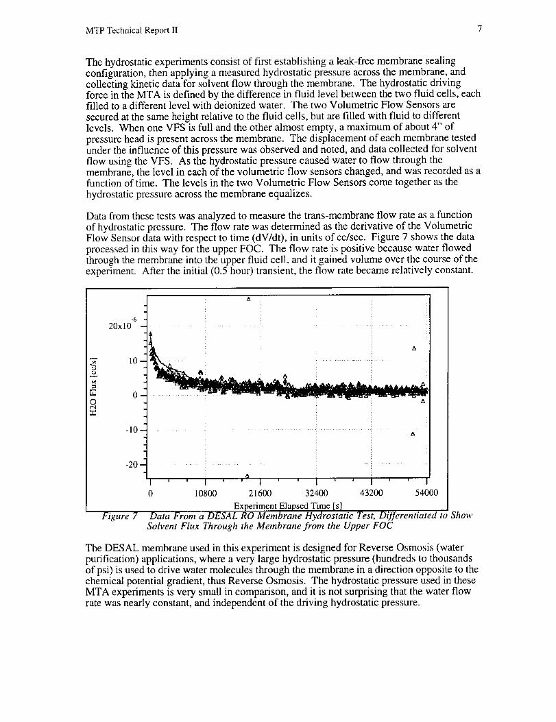
Data from these tests was analyzed to measure the trans-membrane flow rate as a functionof hydrostatic pressure. The flow rate was determined as the derivative of the VolumetricFlow Sensor data with respect to time (dV/dt), in units of cc/sec. Figure 7 shows the dataprocessed in this way for the upper FOC. The flow rate is positive because water flowedthrough the membrane into the upper fluid cell, and it gained volume over the course of the
experiment. After the initial (0.5 hour) transient, the flow rate became relatively constant.
e3
©t"q
20x10
-10
-20
Figure 7
' ' I ' ' I ......0 10800 21600 32400 43200
I
54000
Experiment Elapsed Time Is]Data From a DESAL RO Membrane Hydrostatic Test, Differentiated to Show
Solvent Flux Through the Membrane from the Upper FOC
The DESAL membrane used in this experiment is designed for Reverse Osmosis (water
purification) applications, where a very large hydrostatic pressure (hundreds to thousandsof psi) is used to drive water molecules through the membrane in a direction opposite to thechemical potential gradient, thus Reverse Osmosis. The hydrostatic pressure used in these
MTA experiments is very small in comparison, and it is not surprising that the water flowrate was nearly constant, and independent of the driving hydrostatic pressure.
MTP Technical Report II 8
MEMBRANE EVALUATION ACTIVITIES
Several membranes were tested for hydrostatic flow characteristics, as the membrane sealand refractometer calibration activities allowed. The membranes were evaluated with
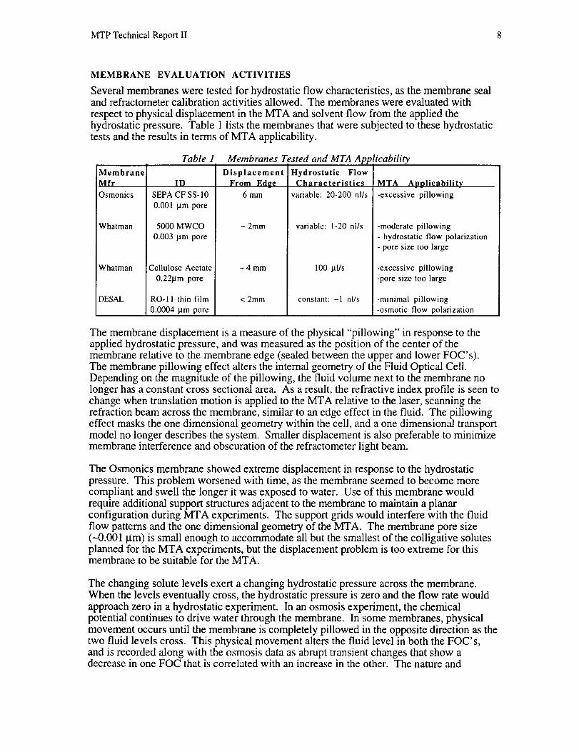
respect to physical displacement in the MTA and solvent flow from the applied thehydrostatic pressure. Table 1 lists the membranes that were subjected to these hydrostatictests and the results in terms of MTA applicability.
Table 1 Membranes Tested and MTA Applicability
Membrane
Mfr
Osmonics
Whatman
Whatman
DESAL
ID
SEPA CF SS-10
0.001 I.tm pore
5000 MWCO
0.003 lam pore
Cellulose Acetate
0.221am pore
RO-I 1 thin film
0.0004 lam pore
Displacement
From Edge
6 mm
- 2mm
~4mm
< 2mm
Hydrostatic Flow
Characteristics
variable: 20-200 nl/s
variable: 1-20 nl/s
100 ktl/s
constant:-1 nl/s
MTA Auplicability
-excessive pillowing
-moderate pillowing
- hydrostatic flow polarization
- pore size too large
-excessive pillowing
-pore size too large
-minimal pillowing
-osmotic flow polarization
The membrane displacement is a measure of the physical "pillowing" in response to theapplied hydrostatic pressure, and was measured as the position of the center of themembrane relative to the membrane edge (sealed between the upper and lower FOC's).The membrane pillowing effect alters the internal geometry of the Fluid Optical Cell.Depending on the magnitude of the pillowing, the fluid volume next to the membrane nolonger has a constant cross sectional area. As a result, the refractive index profile is seen tochange when translation motion is applied to the MTA relative to the laser, scanning therefraction beam across the membrane, similar to an edge effect in the fluid. The pillowingeffect masks the one dimensional geometry within the cell, and a one dimensional transportmodel no longer describes the system. Smaller displacement is also preferable to minimizemembrane interference and obscuration of the refractometer light beam.
The Osmonics membrane showed extreme displacement in response to the hydrostaticpressure. This problem worsened with time, as the membrane seemed to become morecompliant and swell the longer it was exposed to water. Use of this membrane wouldrequire additional support structures adjacent to the membrane to maintain a planar
configuration during MTA experiments. The support grids would interfere with the fluidflow patterns and the one dimensional geometry of the MTA. The membrane pore size
(-0.001 l.tm) is small enough to accommodate all but the smallest of the colligative solutesplanned for the MTA experiments, but the displacement problem is too extreme for thismembrane to be suitable for the MTA.
The changing solute levels exert a changing hydrostatic pressure across the membrane.When the levels eventually cross, the hydrostatic pressure is zero and the flow rate wouldapproach zero in a hydrostatic experiment. In an osmosis experiment, the chemicalpotential continues to drive water through the membrane. In some membranes, physicalmovement occurs until the membrane is completely pillowed in the opposite direction as thetwo fluid levels cross. This physical movement alters the fluid level in both the FOC's,and is recorded along with the osmosis data as abrupt transient changes that show adecrease in one FOC that is correlated with an increase in the other. The nature and
MTP Technical Report II 9
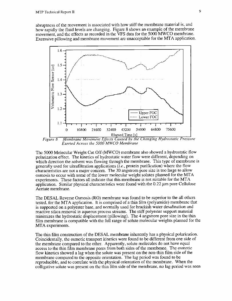
abruptness of the movement is associated with how stiff the membrane material is, andhow rapidly the fluid levels are changing. Figure 8 shows an example of the membranemovement, and the effects as recorded in the VFS data for the 5000 MWCO membrane.
Excessive pillowing and membrane movement are unacceptable for the MTA application.
w
e-
",J
"r"
E
Figure 8
|.6_
!.5
1.4 :
..,. ,:
..,-. "'",..,. .;•.. .... ..
/..- -.-_ ........: _......:.. * " °"_'"°"" _:.,.,..,. .;"'*"
1.2
1.1 I .... I ' ' I ' ' I ' ' I ' ' I ' ' I ' '
0 10800 21600 32400 43200 54000 64800 75600
Elapsed Time Is]Membrane Movement Effects Caused by the Changing Hydrostatic Pressure
Exerted Across the 5000 MWCO Membrane
The 5000 Molecular Weight Cut Off (MWCO) membrane also showed a hydrostatic flow
polarization effect. The kinetics of hydrostatic water flow were different, depending onwhich direction the solvent was flowing through the membrane. This type of membrane isgenerally used for ultrafiltration applications (i.e., protein purification) where the flowcharacteristics are not a major concern. The 30 angstrom pore size is too large to allowosmosis to occur with some of the lower molecular weight solutes planned for the MTAexperiments. These factors all indicate that this membrane is not suitable for the MTAapplication. Similar physical characteristics were found with the 0.22 ILtm pore CelluloseAcetate membrane.
The DESAL Reverse Osmosis (RO) membrane was found to be superior to the all others
tested, for the MTA application. It is comprised of a thin film (polyamide) membrane thatis supported on a polyester base, and normally used for brackish water desalination andreactive silica removal in aqueous process streams. The stiff polyester support materialminimizes the hydrostatic displacement (pillowing). The 4 angstrom pore size in the thinfilm membrane is compatible with the full range of solute molecular weights planned for theMTA experiments.
The thin film construction of the DESAL membrane inherently has a physical polarization.
Coincidentally, the osmotic transport kinetics were found to be different from one side ofthe membrane compared to the other. Apparently, solute molecules do not have equalaccess to the thin film membrane pores from both sides of the membrane. The osmotic
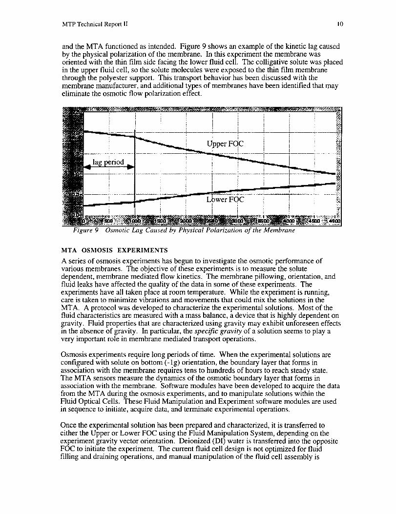
flow kinetics showed a lag when the solute was present on the non-thin film side of themembrane compared to the opposite orientation. The lag period was found to bereproducible, and to correlate with the physical orientation of the membrane. When thecolligative solute was present on the thin film side of the membrane, no lag period was seen
MTP Technical Report II 10
and the MTA functioned as intended. Figure 9 shows an example of the kinetic lag causedby the physical polarization of the membrane. In this experiment the membrane wasoriented with the thin film side facing the lower fluid cell. The colligative solute was placedin the upper fluid cell, so the solute molecules were exposed to the thin film membranethrough the polyester support. This transport behavior has been discussed with themembrane manufacturer, and additional types of membranes have been identified that may
eliminate the osmotic flow polarization effect.
LFOC
Figure 9 Osmotic Lag Caused by Physical Polarizatton of the Membrane
MTA OSMOSIS EXPERIMENTS
A series of osmosis experiments has begun to investigate the osmotic performance ofvarious membranes. The objective of these experiments is to measure the solutedependent, membrane mediated flow kinetics. The membrane pillowing, orientation, and
fluid leaks have affected the quality of the data in some of these experiments. Theexperiments have all taken place at room temperature. While the experiment is running,care is taken to minimize vibrations and movements that could mix the solutions in the
MTA. A protocol was developed to characterize the experimental solutions. Most of thefluid characteristics are measured with a mass balance, a device that is highly dependent ongravity. Fluid properties that are characterized using gravity may exhibit unforeseen effects
in the absence of gravity. In particular, the specific gravity of a solution seems to play avery important role in membrane mediated transport operations.
Osmosis experiments require long periods of time. When the experimental solutions areconfigured with solute on bottom (-lg) orientation, the boundary layer that forms inassociation with the membrane requires tens to hundreds of hours to reach steady state.The MTA sensors measure the dynamics of the osmotic boundary layer that forms inassociation with the membrane. Software modules have been developed to acquire the datafrom the MTA during the osmosis experiments, and to manipulate solutions within theFluid Optical Cells. These Fluid Manipulation and Experiment software modules are usedin sequence to initiate, acquire data, and terminate experimental operations.
Once the experimental solution has been prepared and characterized, it is transferred toeither the Upper or Lower FOC using the Fluid Manipulation System, depending on theexperiment gravity vector orientation. Deionized (DI) water is transferred into the oppositeFOC to initiate the experiment. The current fluid cell design is not optimized for fluidfilling and draining operations, and manual manipulation of the fluid cell assembly is
MTPTechnicalReportII 11
requiredto insurethatcompletefilling occurs(notrappedbubbles).Theinitiationof anexperimentcorrespondsto maximumhydrostaticpressureacrossthemembrane,andmaximummembranepillowing in onedirection.Thisconfigurationsetsthemembraneinaninitially rigid position. As osmosisdriveswaterthroughthemembrane,the levelsin theVolumetricFlowSensorschange,andarerecordedasexperimentaldataalongwith theambienttemperature.RefractiveIndexprofile imagesarealsoacquiredatregularintervalsoverthecourseof theexperiment.
Fluidmanipulationscriptshavebeendevelopedto fill theUpperandLowerFOC's to pre-definedlevelsin preparationfor anexperiment.TheFOCcontainingthesoluteis alwaysfilled to theminimallevel (-0.2 cc),andthepurewaterFOCis filled to themaximallevel.This initial configurationexertsthemaximumhydrostaticpressureacrossthemembraneatthestartof anexperiment,about4 inchesof hydrostatichead.TheFluid ManipulationSystemandassociatedsoftwarearedescribedin aseparatesectionof thisreport.
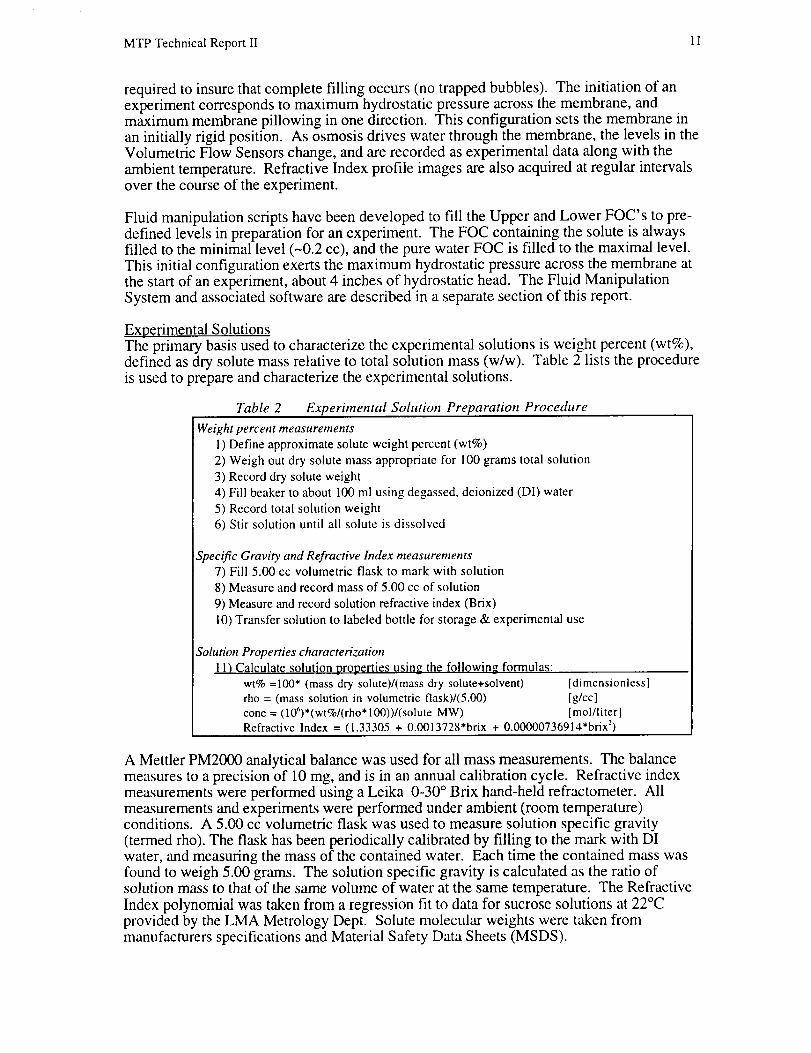
Experimental SolutionsThe primary basis used to characterize the experimental solutions is weight percent (wt%),defined as dry solute mass relative to total solution mass (w/w). Table 2 lists the procedureis used to prepare and characterize the experimental solutions.
Table 2 Experimental Solution Preparation Procedure
Weight percent measurements1) Define approximate solute weight percent (wt%)2) Weigh out dry solute mass appropriate for 100 grams total solution3) Record dry solute weight4) Fill beaker to about I00 ml using degassed, deionized (DI) water5) Record total solution weight6) Stir solution until all solute is dissolved
Specific Gravity and Refractive Index measurements7) Fill 5.00 cc volumetric flask to mark with solution8) Measure and record mass of 5.00 cc of solution9) Measure and record solution refractive index (Brix)I0) Transfer solution to labeled bottle for storage & experimental use
Solution Properties characterizationI1) Calculate solution properties using the foll0wi0g formulas:
wt% =100" (mass dry solute)/(mass dry solute+solvent) [dimensionless]rho = (mass solution in volumetric flask)l(5.00) [g/cc]conc = (106)*(wt%/(rho*100))/(solute MW) [mol/liter]Refractive Index = (1.33305 + 0.0013728*brix + 0.00000736914*brix 2)
A Mettler PM2000 analytical balance was used for all mass measurements. The balancemeasures to a precision of 10 mg, and is in an annual calibration cycle. Refractive indexmeasurements were performed using a Leika 0-30 ° Brix hand-held refractometer. Allmeasurements and experiments were performed under ambient (room temperature)conditions. A 5.00 cc volumetric flask was used to measure solution specific gravity(termed rho). The flask has been periodically calibrated by filling to the mark with DIwater, and measuring the mass of the contained water. Each time the contained mass wasfound to weigh 5.00 grams. The solution specific gravity is calculated as the ratio ofsolution mass to that of the same volume of water at the same temperature. The Refractive
Index polynomial was taken from a regression fit to data for sucrose solutions at 22°Cprovided by the LMA Metrology Dept. Solute molecular weights were taken from
manufacturers specifications and Material Safety Data Sheets (MSDS).
MTP Technical Report II 12
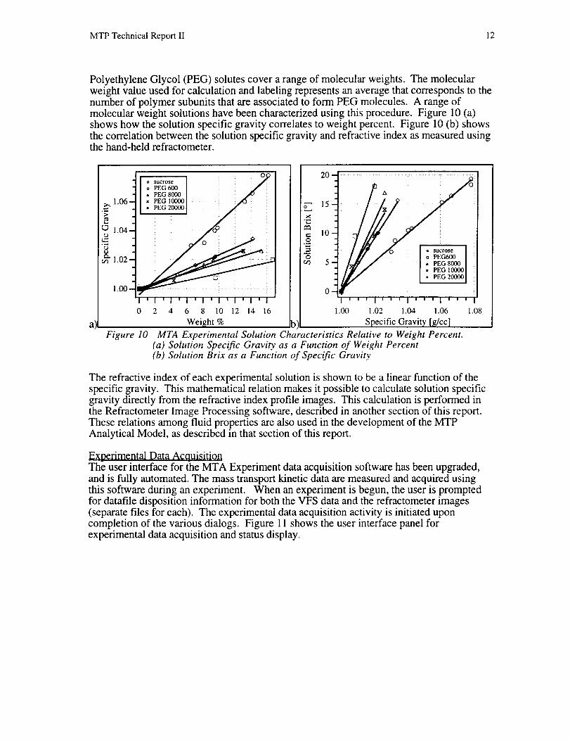
Polyethylene Glycol (PEG) solutes cover a range of molecular weights. The molecularweight value used for calculation and labeling represents an average that corresponds to thenumber of polymer subunits that are associated to form PEG molecules. A range ofmolecular weight solutions have been characterized using this procedure. Figure 10 (a)shows how the solution specifc gravity correlates to weight percent. Figure 10 (b) showsthe correlation between the solution specific gravity and refractive index as measured usingthe hand-held refractometer.
* sucrose
"tl " PEG 8000 I
1.06'-'] I x PEG 100001 ...... i '_ ....
,.04q /g -: o
I '1 'l 'l '1 '1 '1 '1 '1
0 2 4 6 8 10 12 14 16
Weight %
Figure 10
1.00 1,02 1.04 ! .06
Specific Gravity [_/cc]
MTA Experimental Solution Characteristics Relative to Weight Percent.(a) Solution Specific Gravity as a Function of Weight Percent
(b) Solution Brix as a Function of Specific Gravity
20 --I ............................
A o
15
_ IO._
I!/ /- I oPEG6OOI
S0 ; / I, P_SOOO I
/ii¢/ I I_ PEG_ooooI
........................... I .' "EG2_I
I I I I I I I I I J I I I I I
1.08
The refractive index of each experimental solution is shown to be a linear function of thespecific gravity. This mathematical relation makes it possible to calculate solution specificgravity directly from the refractive index profile images. This calculation is performed inthe Refractometer Image Processing software, described in another section of this report.These relations among fluid properties are also used in the development of the MTPAnalytical Model, as described in that section of this report.
Experimental Data Acquisition
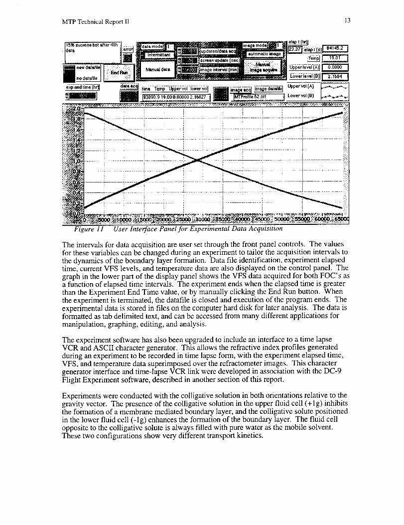
The user interface for the MTA Experiment data acquisition software has been upgraded,and is fully automated. The mass transport kinetic data are measured and acquired usingthis software during an experiment. When an experiment is begun, the user is promptedfor datafile disposition information for both the VFS data and the refractometer images(separate files for each). The experimental data acquisition activity is initiated uponcompletion of the various dialogs. Figure 11 shows the user interface panel forexperimental data acquisition and status display.
MTP Technical Report II 13
Figure 11 User Interface Panel for Experimental Data Acquisition
The intervals for data acquisition are user set through the front panel controls. The valuesfor these variables can be changed during an experiment to tailor the acquisition intervals tothe dynamics of the boundary layer formation. Data file identification, experiment elapsedtime, current VFS levels, and temperature data are also displayed on the control panel. Thegraph in the lower part of the display panel shows the VFS data acquired for both FOC's asa function of elapsed time intervals. The experiment ends when the elapsed time is greaterthan the Experiment End Time value, or by manually clicking the End Run button. Whenthe experiment is terminated, the datafile is closed and execution of the program ends. Theexperimental data is stored in files on the computer hard disk for later analysis. The data isformatted as tab delimited text, and can be accessed from many different applications for
manipulation, graphing, editing, and analysis.
The experiment software has also been upgraded to include an interface to a time lapseVCR and ASCII character generator. This allows the refractive index profiles generatedduring an experiment to be recorded in time lapse form, with the experiment elapsed time,VFS, and temperature data superimposed over the refractometer images. This charactergenerator interface and time-lapse VCR link were developed in association with the DC-9Flight Experiment software, described in another section of this report.
Experiments were conducted with the colligative solution in both orientations relative to thegravity vector. The presence of the colligative solution in the upper fluid cell (+ 1g) inhibitsthe formation of a membrane mediated boundary layer, and the colligative solute positionedin the lower fluid cell (- 1g) enhances the formation of the boundary layer. The fluid cellopposite to the colligative solute is always filled with pure water as the mobile solvent.These two configurations show very different transport kinetics.
MTP Technical Report II 14
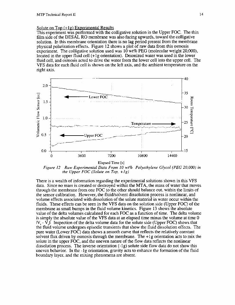
Solute on Top (+ 1g) Experimental ResultsThis experiment was performed with the colligative solution in the Upper FOC. The thinfilm side of the DESAL RO membrane was also facing upwards, toward the colligativesolution. In this membrane orientation there is no lag period present from the membranephysical polarization effects. Figure 12 shows a plot of raw data from this osmosisexperiment. The colligative solution used was 10 wt% PEG (molecular weight 20,000),located in the upper fluid cell (+ 1g orientation). Deionized water was used in the lowerfluid cell, and osmosis acted to drive the water from the lower cell into the upper cell. TheVFS data for each fluid cell is shown on the left axis, and the ambient temperature on the
right axis.
2.0
,-ff
1.5e-,
r,,¢3
o
1.0
I-
E
;_ 0.5
0.0
--_ Lower FOC
Temperature "'-
_'_-.,, Upper FOC __
_S -¸._'_
I I I
0 3600 7200 10800 14400
Figure 12
Elapsed Time [s]
-40
-35
7_0
-30
-25 E
o
-20
15
Raw Experimental Data From 10 wt% Polyethylene Glycol (PEG 20,000) inthe Upper FOC (Solute on Top, + lg)
There is a wealth of information regarding the experimental solutions shown in this VFSdata. Since no mass is created or destroyed within the MTA, the mass of water that movesthrough the membrane from one FOC to the other should balance out, within the limits ofthe sensor calibration. However, the fluid/solvent dissolution process is nonlinear, andvolume effects associated with dissolution of the solute material in water occur within the
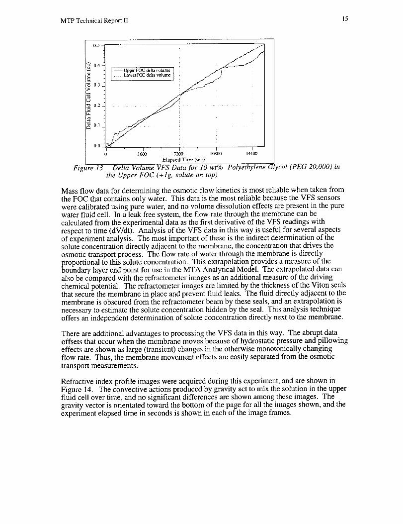
fluids. These effects can be seen in the VFS data on the solution side (Upper FOC) of themembrane as small bumps in the fluid volume kinetics. Figure 13 shows the absolutevalue of the delta volumes calculated for each FOC as a function of time. The delta volume
is simply the absolute value of the VFS data at an elapsed time minus the volume at time 0IV, - Vol. Inspection of the delta volume data for the solute side (Upper FOC) shows thatthe fluid volume undergoes episodic transients that show the fluid dissolution effects. Thepure water (Lower FOC) data shows a smooth curve that reflects the relatively constantsolvent flux driven by osmosis through the membrane. The + 1g orientation acts to mix the
solute in the upper FOC, and the uneven nature of the flow data reflects the nonlineardissolution process. The inverse orientation (-lg) solute side flow data do not show thisuneven behavior. In the -lg orientation, gravity acts to enhance the formation of the fluidboundary layer, and the mixing phenomena are absent.
MTP Technical Report II 15
0_5 "-t
°.41t
"_ 02-_
0.0 "1
Figure 13
I I 1 I
0 3600 7200 10800 14400
Elapsed Titre (sec)
Delta Volume VFS Data for 10 wt% Polyethylene Glycol (PEG 20,000) in
the Upper FOC (+lg, solute on top)
Mass flow data for determining the osmotic flow kinetics is most reliable when taken fromthe FOC that contains only water. This data is the most reliable because the VFS sensorswere calibrated using pure water, and no volume dissolution effects are present in the purewater fluid cell. In a leak free system, the flow rate through the membrane can becalculated from the experimental data as the first derivative of the VFS readings with
respect to time (dV/dt). Analysis of the VFS data in this way is useful for several aspectsof experiment analysis. The most important of these is the indirect determination of thesolute concentration directly adjacent to the membrane, the concentration that drives theosmotic transport process. The flow rate of water through the membrane is directly
proportional to this solute concentration. This extrapolation provides a measure of theboundary layer end point for use in the MTA Analytical Model. The extrapolated data canalso be compared with the refractometer images as an additional measure of the driving
chemical potential. The refractometer images are limited by the thickness of the Viton sealsthat secure the membrane in place and prevent fluid leaks. The fluid directly adjacent to themembrane is obscured from the refractometer beam by these seals, and an extrapolation is
necessary to estimate the solute concentration hidden by the seal. This analysis techniqueoffers an independent determination of solute concentration directly next to the membrane.
There are additional advantages to processing the VFS data in this way. The abrupt dataoffsets that occur when the membrane moves because of hydrostatic pressure and pillowing
effects are shown as large (transient) changes in the otherwise monotonically changingflow rate. Thus, the membrane movement effects are easily separated from the osmotic
transport measurements.
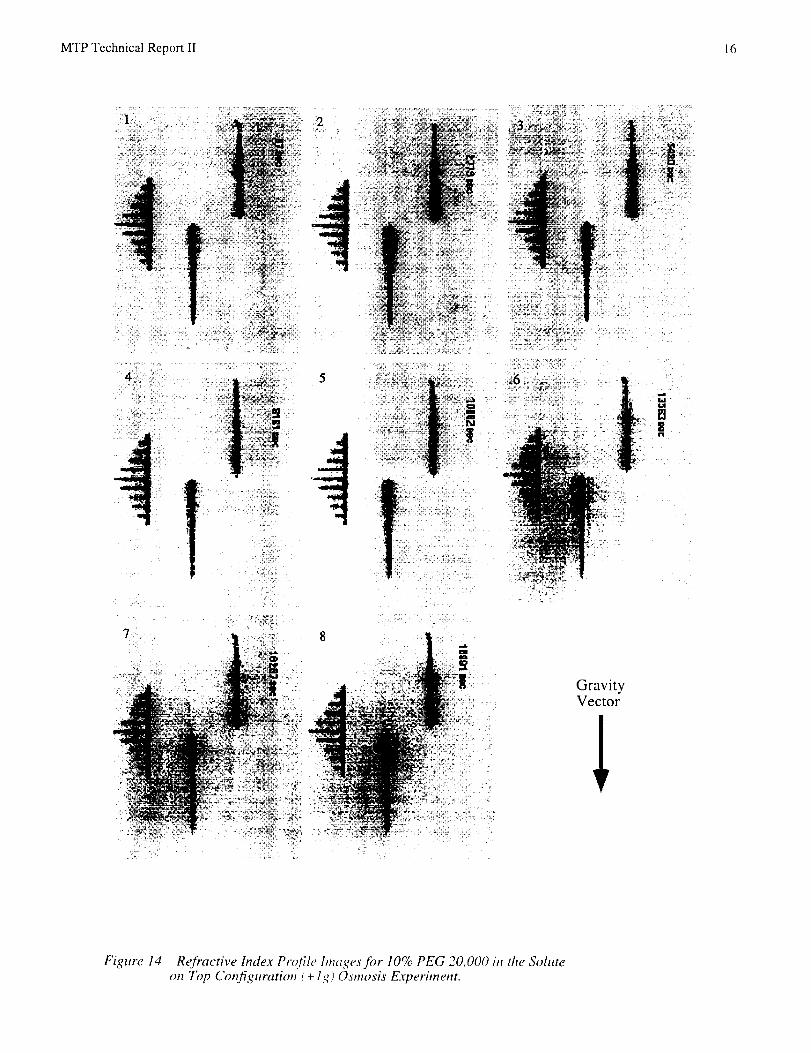
Refractive index profile images were acquired during this experiment, and are shown inFigure 14. The convective actions produced by gravity act to mix the solution in the upperfluid cell over time, and no significant differences are shown among these images. The
gravity vector is orientated toward the bottom of the page for all the images shown, and theexperiment elapsed time in seconds is shown in each of the image frames.
MTP Technical Report II 16
7 8
GravityVector
Figure 14 Refractive hldex Profile hna_,es ]br 10% PEG 20.00¢) i_1the Soluteon Top Configuration (+ I g ) Osmosis Experiment.
MTP Technical Report II 17
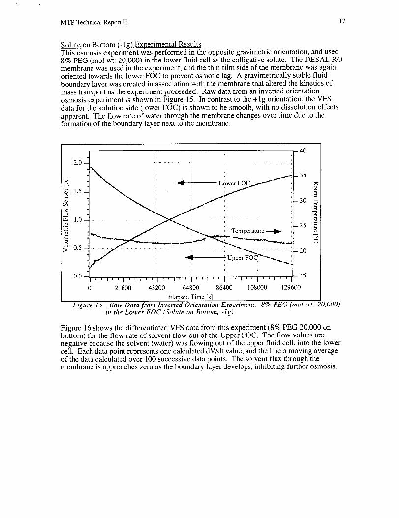
Solute on Bottom (-1 g) Experimental ResultsThis osmosis experiment was performed in the opposite gravimetric orientation, and used8% PEG (mol wt: 20,000) in the lower fluid cell as the colligative solute. The DESAL ROmembrane was used in the experiment, and the thin film side of the membrane was againoriented towards the lower FOC to prevent osmotic lag. A gravimetrically stable fluidboundary layer was created in association with the membrane that altered the kinetics of
mass transport as the experiment proceeded. Raw data from an inverted orientationosmosis experiment is shown in Figure 15. In contrast to the + lg orientation, the VFSdata for the solution side (lower FOC) is shown to be smooth, with no dissolution effects
apparent. The flow rate of water through the membrane changes over time due to theformation of the boundary layer next to the membrane.
O
y.
E
O
2.0-
1.5 '
|.0--
o.s :
0.0-,, i, ,i ,, i, ,i ,, i, , i, ,i ,, j, ,i ,, i, ,i , ,
0 21600 43200 64800 86400 108000
--40
--35
--30
--25
--20
- 15
129600
Elapsed Time [s]
O
#
o
Figure 15 Raw Data from Inverted Orientation Experiment. 8% PEG (mol wt: 20,000)in the Lower FOC (Solute on Bottom, -lg)
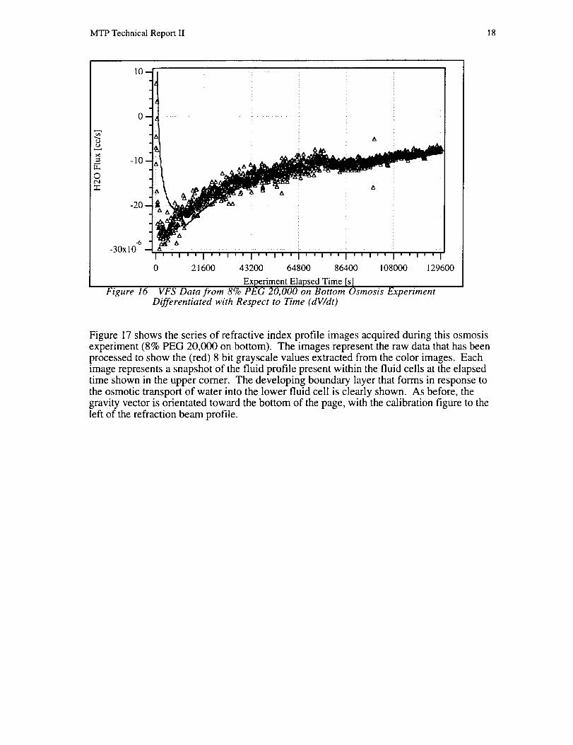
Figure 16 shows the differentiated VFS data from this experiment (8% PEG 20,000 onbottom) for the flow rate of solvent flow out of the Upper FOC. The flow values arenegative because the solvent (water) was flowing out of the upper fluid cell, into the lowercell. Each data point represents one calculated dV/dt value, and the line a moving averageof the data calculated over I00 successive data points. The solvent flux through themembrane is approaches zero as the boundary layer develops, inhibiting further osmosis.
MTP Technical Report II 18
e._
©¢",1
10-
.
-10 -
-20 -
-6
-30x10
Figure 16
! •
, ,t .'l '' I'' I'' I' '1' 'i ''1 '' i .... I' '
0 21600 43200 64800 86400 108000 129600
Experiment Elapsed Time Is]VFS Data from 8% PEG 20,000 on Bottom Osmosis Experiment
Differentiated with Respect to Time (dV/dt)
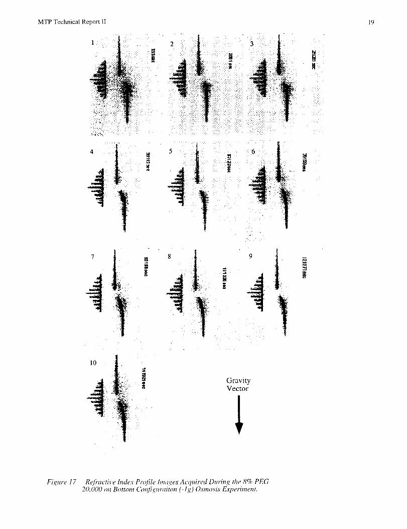
Figure 17 shows the series of refractive index profile images acquired during this osmosis
experiment (8% PEG 20,000 on bottom). The images represent the raw data that has been
processed to show the (red) 8 bit grayscale values extracted from the color images. Each
image represents a snapshot of the fluid profile present within the fluid cells at the elapsed
time shown in the upper comer. The developing boundary layer that forms in response to
the osmotic transport of water into the lower fluid cell is clearly shown. As before, the
gravity vector is orientated toward the bottom of the page, with the calibration figure to the
left of the refraction beam profile.
MTPTechnicalReportII 19
m
4
!7
U_
5
9
i
il
.m
10
GravityVector
Figure 17 Rej)'active Index Profile lmaq, es Acquired During the 8% PEG20,000 on Bottom Col!/_guraiton (-l g) Osmosis Experiment.
MTP Technical Report II 20
MTA FLUID MANIPULATION SYSTEMS (FMS) DEVELOPMENT
The Fluid Manipulation System was developed to sequence fluid valves and enableautomated fluid transfers within the MTA. The use of the FMS became necessary to
eliminate convective interference's that were occurring in the lower fluid cell. Duringosmosis experiments where the colligative solution was positioned in the lower fluid cell, itbecame apparent that gravity induced convective flows were mixing the fluid boundarylayer as it developed adjacent to the membrane. The MTA had to be reconfigured toeliminate the convective interference, a development that required major changes in the fluidsystem design. The new instrument configuration represents a quantum evolution in theMTA fluid handling capabilities, and is more flight like than the previous fluidconfiguration.
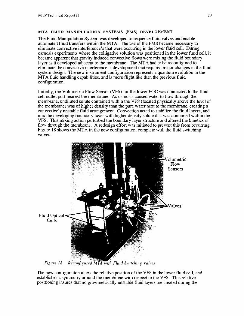
Initially, the Volumetric Flow Sensor (VFS) for the lower FOC was connected to the fluidcell outlet port nearest the membrane. As osmosis caused water to flow through themembrane, undiluted solute contained within the VFS (located physically above the level ofthe membrane) was of higher density than the pure water next to the membrane, creating aconvectively unstable fluid arrangement. Convection acted to stabilize the fluid layers, andmix the developing boundary layer with higher density solute that was contained within theVFS. This mixing action perturbed the boundary layer structure and altered the kinetics offlow through the membrane. A redesign effort was initiated to prevent this from occurring.Figure 18 shows the MTA in the new configuration, complete with the fluid switchingvalves.
FlowSensors
Fluid OCells
Figure 18_:1_ _ i I! • •
Reconfigured MTA with Fluid Switching Valves
The new configuration alters the relative position of the VFS in the lower fluid cell, andestablishes a symmetry around the membrane with respect to the VFS. This relativepositioning insures that no gravimetrically unstable fluid layers are created during the
MTP Technical Report II 21
osmosis experiments. Simply stated, the Volumetric Flow Sensors are now located at thefarthest points from the membrane in both the Upper and Lower FOC's. The newconfiguration is more complex than the prior arrangement, and requires valves to insurethat fluids flow sequentially into the FOC's and VFS in preparation for an experiment.
Both of the fluid cells must be filled from the lower (inlet) port in a lg environment. To
accomplish the filling operation, the valves are sequenced to first direct the experimentalfluids into the upper fluid cell and VFS, then into the lower fluid cell and VFS. Theposition of the upper VFS remains at the (upper) outlet port for the upper cell, and is
naturally filled from the bottom. The lower VFS was moved to a position near the lowerfluid cell inlet port, and requires valves to insure that the fluid cell is filled prior to the VFS.Four valves are required for these fluid manipulations. The valves are electrically operated,and a collection of electrical interface circuits were developed to allow computer actuation
of the valves in sequences appropriate for the fluid manipulations. The MTA fluid flowschematic diagram is shown in the Fluid Manipulation Software section of this report.
The valve electrical interface was extended to include the circuit drivers for control of the
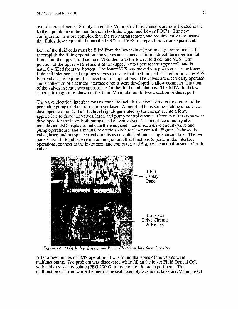
peristaltic pumps and the refractometer laser. A modified transistor switching circuit wasdeveloped to amplify the TI'L level signals generated by the computer into a formappropriate to drive the valves, laser, and pump control circuits. Circuits of this type weredeveloped for the laser, both pumps, and eleven valves. The interface circuitry alsoincludes an LED display to indicate the energized state of each drive circuit (valve andpump operations), and a manual override switch for laser control. Figure 19 shows thevalve, laser, and pump electrical circuits as consolidated into a single circuit box. The twoparts shown fit together to form an integral unit that functions to perform the interfaceoperations, connect to the instrument and computer, and display the actuation state of eachvalve.
LED
DisplayPanel
TransistorCircuits
& Relays
Figure 19 MTA Valve, Laser, and Pump Electrical Interface Circuitry
After a few months of FMS operation, it was found that some of the valves weremalfunctioning. The problem was discovered while filling the lower Fluid Optical Cellwith a high viscosity solute (PEG 20000) in preparation for an experiment. Thismalfunction occurred while the membrane seal assembly was in the latex and Viton gasket
MTPTechnicalReportII 22
configuration,andpromptedfurtherdevelopmentof theseal.Thelower fluid cell outletvalvehadbecomestuckin theclosedpositionwhile thefluid pumpswerepumpingsolutein, andcauseda higherthannormalpressureto beexertedacrossthemembrane.Thepressurecausedthemembraneto comeloosefrom its seatbetweentheUpperandLowerFOC's,a"blownmembrane".It waslaterdeterminedthatthevalvemalfunctiondid nothappenall atonce,it occurredgraduallyoverthecourseof severalexperiments.Initially,the increasedpressurecausedthemembraneto bedisplacedwithin its sealmorethanusual.Theexcessivemembranepillowing thatwasobservedwasattributedto thehighviscositysolutethatwasbeingused.Eventuallythevalvebecamecompletelystuckin theclosedposition,andthemembranecameloosefrom its sealbetweentheFOC's. Severalfluidmanipulations,blownmembranes,andFOCrebuildcyclesoccurredbeforeit wasrealizedthatthevalvesweremalfunctioning.
Thevalveproblemwasinvestigatedandall valvesin theMTA tested.Someof theMTAvalvesshowedleakagein "closed"paths,while othervalveswouldnotswitch fluid pathswhenactuated.In all casesthesoftwareandelectricalcircuitry showednoproblems.Indiscussionswith thevalvevendor(LeeValves),it wasdeterminedthatamaterialusedtoconstructthevalveseat(Neoprene)isnotcompatiblefor continuouscontactwith aqueoussolutions.Apparently,Neoprenehasatendencyto absorbsmallamountsof waterandswell,apropertythatis not listedin thematerialsselectionsectionof theLeecatalog.WhentheNeoprenevalveseatmaterialswells,it canbecomelodgedwithin theactuationpath,ornotseatcompletelyagainstthefluid valveports. Thesevalvesarethenpronetoleakageand/orstickingin openorclosedpositions.Themalfunctioningvalvesseemtobecomeoperationalagainoncetheabsorbedwaterhasevaporatedfrom theNeopreneseatmaterial.
TheLeeValveCompanyrecommendedreplacementvalves that have valve seatsconstructed using an aqueous compatible material (Teflon). New valves were ordered toreplace the current valves, but have not yet been received. In the interim, three of the fourmalfunctioning valves have been replaced with spares (also Neoprene valve seats). Thisallows the MTA experiments to continue until the new valves are received. The initial(Neoprene seat) valves worked fine for about three months before the malfunctionoccurred. The new replacement valves should be received before the spare valvesmalfunction.
FMS SOFTWARE DEVELOPMENT
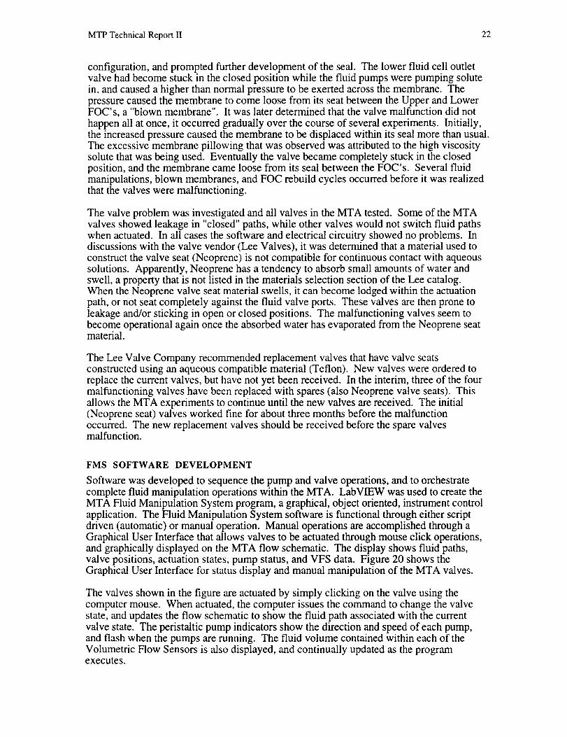
Software was developed to sequence the pump and valve operations, and to orchestratecomplete fluid manipulation operations within the MTA. LabVIEW was used to create theMTA Fluid Manipulation System program, a graphical, object oriented, instrument controlapplication. The Fluid Manipulation System software is functional through either scriptdriven (automatic) or manual operation. Manual operations are accomplished through aGraphical User Interface that allows valves to be actuated through mouse click operations,and graphically displayed on the MTA flow schematic. The display shows fluid paths,valve positions, actuation states, pump status, and VFS data. Figure 20 shows theGraphical User Interface for status display and manual manipulation of the MTA valves.
The valves shown in the figure are actuated by simply clicking on the valve using the
computer mouse. When actuated, the computer issues the command to change the valvestate, and updates the flow schematic to show the fluid path associated with the currentvalve state. The peristaltic pump indicators show the direction and speed of each pump,and flash when the pumps are running. The fluid volume contained within each of theVolumetric Flow Sensors is also displayed, and continually updated as the programexecutes.
MTP Technical Report II 23
o 5o IOOi
MTA Fluid Manipulation Systen_
Pump & Valve status & Control Panel]
Figure 20 MTA Fluid Manipulation System Graphical User Interface
The fluid manipulation scripts for automated sequences of operations consist ofindependent lines of tab delimited ASCII text. These lines can be generated using a wordprocessor, spreadsheet application, or LabVIEW editor. Sequences of the script lines areput together to form complete fluid manipulation scripts. Scripts have been written toperform all of the fluid manipulation functions within the MTA, and include fluid cell fillingand draining operations, fluid cell and tubing purges, refractometer calibration, andVolumetric Flow Sensor calibration.
Execution of the fluid scripts is accomplished through a hierarchy of software modules, or
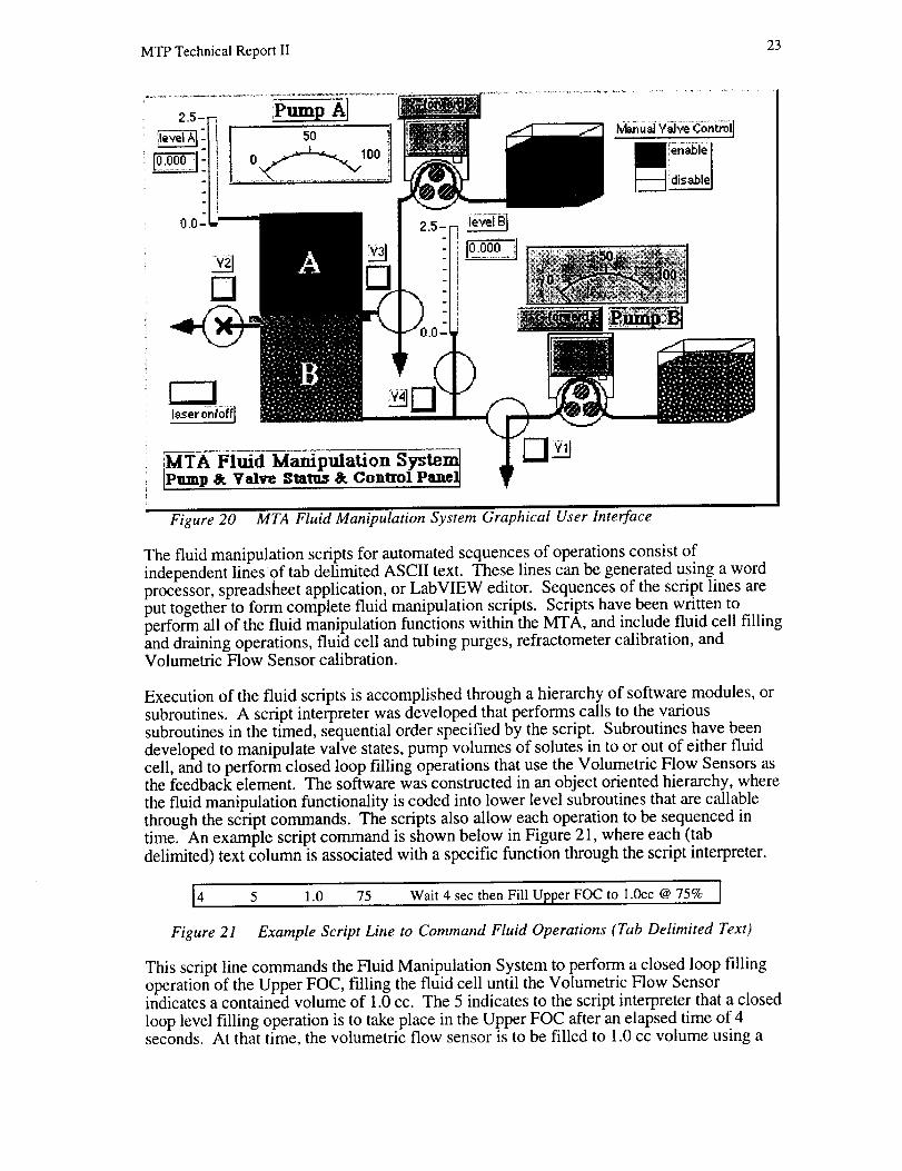
subroutines. A script interpreter was developed that performs calls to the varioussubroutines in the timed, sequential order specified by the script. Subroutines have beendeveloped to manipulate valve states, pump volumes of solutes in to or out of either fluidcell, and to perform closed loop filling operations that use the Volumetric Flow Sensors asthe feedback element. The software was constructed in an object oriented hierarchy, wherethe fluid manipulation functionality is coded into lower level subroutines that are callablethrough the script commands. The scripts also allow each operation to be sequenced intime. An example script command is shown below in Figure 21, where each (tab
delimited) text column is associated with a specific function through the script interpreter.
4 5 l.O 75 Wait 4 sec then Fill Upper FOC to 1.0cc @ 75% I
Figure 21 Example Script Line to Command Fluid Operations (Tab Delimited Text)
This script line commands the Fluid Manipulation System to perform a closed loop fillingoperation of the Upper FOC, filling the fluid cell until the Volumetric Flow Sensorindicates a contained volume of 1.0 cc. The 5 indicates to the script interpreter that a closedloop level filling operation is to take place in the Upper FOC after an elapsed time of 4seconds. At that time, the volumetric flow sensor is to be filled to 1.0 cc volume using a
MTP Technical Report II 24
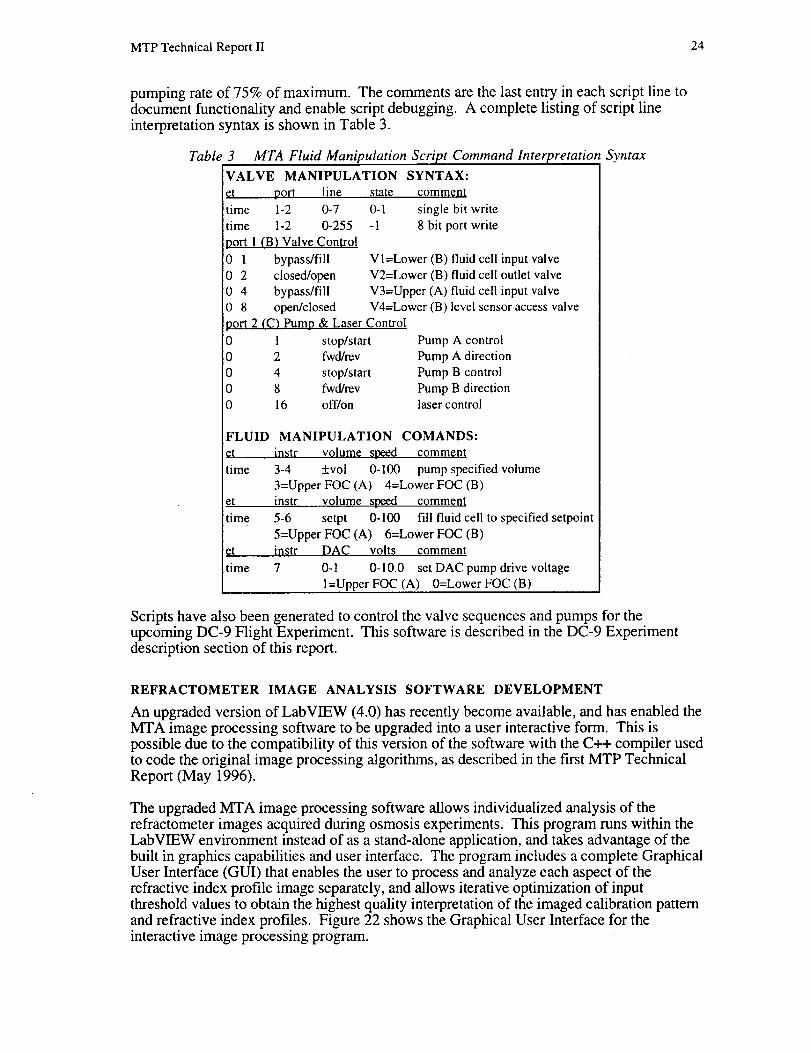
pumping rate of 75% of maximum. The comments are the last entry in each script line todocument functionality and enable script debugging. A complete listing of script lineinterpretation syntax is shown in Table 3.
Table 3 MTA Fluid Manipulation Script Command Interpretation Syntax
VALVE MANIPULATION SYNTAX:
e_ port line state comment
time 1-2 0-7 0-1 single bit write
time 1-2 0-255 -1 8 bit port write
port 1 (B) Valve Control
0 1 bypass/fill
0 2 closed/open
0 4 bypass/fill
0 8 open/closed
port 2 (C) Pump & Laser Control
0 1 stop/start0 2 fwd/rev
0 4 stop/start0 8 fwd/rev
0 16 off/on
Vl=Lower (B) fluid cell input valve
V2=Lower (B) fluid cell outlet valve
V3=Upper (A) fluid cell input valveV4=Lower (B) level sensor access valve
Pump A control
Pump A direction
Pump B control
Pump B directionlaser control
FLUID MANIPULATION COMANDS:
et instr volume s_tzeed comment
time 3-4 +vol 0-100 pump specified volume
3=Upper FOC (A) 4=Lower FOC (B)et instr volume speed comment
time 5-6 setpt 0-100 fill fluid cell to specified setpoint
5=Upper FOC (A) 6=Lower FOC (B)et instr DAC volts comment
time 7 0-1 0-10.0 set DAC pump drive voltage
l=Upper FOC (A) 0=Lower FOC (B)
Scripts have also been generated to control the valve sequences and pumps for theupcoming DC-9 Flight Experiment. This software is described in the DC-9 Experimentdescription section of this report.
REFRACTOMETER IMAGE ANALYSIS SOFTWARE DEVELOPMENT
An upgraded version of LabVIEW (4.0) has recently become available, and has enabled theMTA image processing software to be upgraded into a user interactive form. This ispossible due to the compatibility of this version of the software with the C++ compiler usedto code the original image processing algorithms, as described in the first MTP TechnicalReport (May 1996).
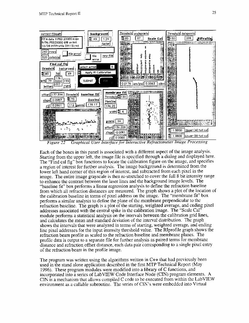
The upgraded MTA image processing software allows individualized analysis of therefractometer images acquired during osmosis experiments. This program runs within theLabVIEW environment instead of as a stand-alone application, and takes advantage of thebuilt in graphics capabilities and user interface. The program includes a complete GraphicalUser Interface (GUI) that enables the user to process and analyze each aspect of therefractive index profile image separately, and allows iterative optimization of inputthreshold values to obtain the highest quality interpretation of the imaged calibration patternand refractive index profiles. Figure 22 shows the Graphical User Interface for theinteractive image processing program.
MTP Technical Report II 25
off_e_ Thresho]d fitl_
_iopel_l _ Baseline]
Figure 22
_ _dRIProfileJ
membrane fitl
Threshold 30 t
Graphical User Interface for Interactive Refractometer hnage Processing
Each of the boxes in this panel is associated with a different aspect of the image analysis.Starting from the upper left, the image file is specified through a dialog and displayed here.The "Find cal fig" box functions to locate the calibration figure on the image, and specifiesa region of interest for further analysis. The image background is determined from thelower left hand comer of this region of interest, and subtracted from each pixel in theimage. The entire image grayscale is then re-stretched to cover the full 8 bit intensity rangeto enhance the contrast between the laser lines and the background image levels. The
"baseline fit" box performs a linear regression analysis to define the refraction baselinefrom which all refraction distances are measured. The graph shows a plot of the location of
the calibration baseline in terms of pixel address on the image. The "membrane fit" boxperforms a similar analysis to define the plane of the membrane perpendicular to therefraction baseline. The graph is a plot of the starting, weighted average, and ending pixeladdresses associated with the central spike in the calibration image. The "Scale Cal"
module performs a statistical analysis on the intervals between the calibration grid lines,and calculates the mean and standard deviation of the interval distribution. The graphshows the intervals that were analyzed in terms of starting, weighted average, and ending
line pixel addresses for the input intensity threshold value. The RIprofile graph shows therefraction beam profile as scaled to the refraction baseline and membrane planes. Theprofile data is output to a separate file for further analysis as paired terms for membranedistance and refraction offset distance, each data pair corresponding to a single pixel entry
of the refraction beam in the profile image.
The program was written using the algorithms written in C++ that had previously beenused in the stand alone application described in the first MTP Technical Report (May
1996). These program modules were modified into a library of C functions, andincorporated into a series of LabVIEW Code Interface Node (CIN) program elements. ACIN is a mechanism that allows compiled C code to be executed from within the LabVIEWenvironment as a callable subroutine. The series of CIN's were embedded into Virtual
MTP Technical Report II 26
Instruments (LabVIEW subroutines), and structured together to enable end to end
processing of the MTA refractive index profile images. This custom processing abilityallows precise dimensional calibration of refractometer images by processing the images tocorrect for background level and laser intensity variations over the entire image. Figure 23
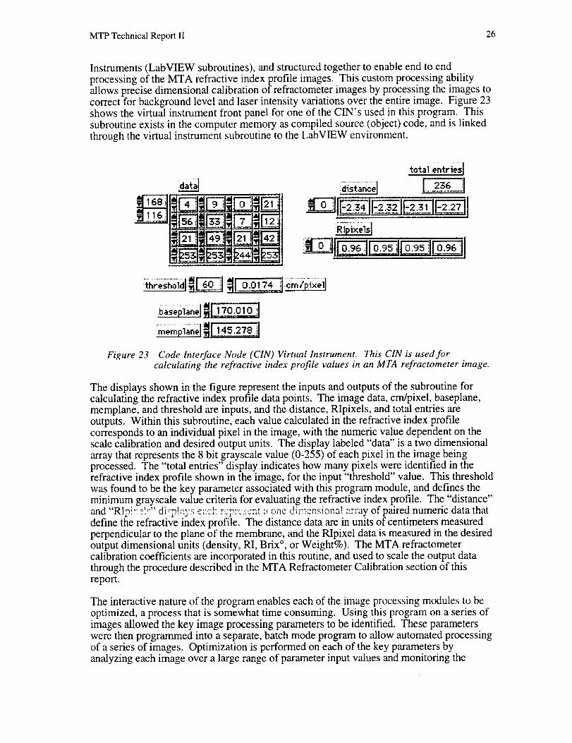
shows the virtual instrument front panel for one of the CIN' s used in this program. Thissubroutine exists in the computer memory as compiled source (object) code, and is linkedthrough the virtual instrument subroutine to the LabVIEW environment.
t0_,lemri'S l
Figure 23 Code Interface Node (CIN) Virtual Instrument. This CIN is used forcalculating the refractive index profile values in an MTA refractometer image.
The displays shown in the figure represent the inputs and outputs of the subroutine forcalculating the refractive index profile data points. The image data, cm/pixel, baseplane,memplane, and threshold are inputs, and the distance, Rlpixels, and total entries areoutputs. Within this subroutine, each value calculated in the refractive index profilecorresponds to an individual pixel in the image, with the numeric value dependent on thescale calibration and desired output units. The display labeled "data" is a two dimensionalarray that represents the 8 bit grayscale value (0-255) of each pixel in the image beingprocessed. The "total entries" display indicates how many pixels were identified in therefractive index profile shown in the image, for the input "threshold" value. This thresholdwas found to be the key parameter associated with this program module, and defines theminimum grayscale value criteria for evaluating the refractive index profile. The "distance"and "RIp!'_1_:" di_!a2,'s e:-,_l_ r_?:_'::,_at a one dimensiona! array of paired numeric data thatdefine the refractive index profile. The distance data are in units of centimeters measuredperpendicular to the plane of the membrane, and the RIpixel data is measured in the desiredoutput dimensional units (density, RI, Brix °, or Weight%). The MTA refractometercalibration coefficients are incorporated in this routine, and used to scale the output datathrough the procedure described in the MTA Refractometer Calibration section of this
report.
The interactive nature of the program enables each of the image processing modules to beoptimized, a process that is somewhat time consuming. Using this program on a series of
images allowed the key image processing parameters to be identified. These parameterswere then programmed into a separate, batch mode program to allow automated processingof a series of images. Optimization is performed on each of the key parameters byanalyzing each image over a large range of parameter input values and monitoring the
MTPTechnicalReportII 27
qualityof theanalysisasshownbytheoutputvariables.Forexample,themagnitudeofthestandarddeviationfrom themeanisusedto optimizethescalecalibrationanalysis.Thethresholdvaluethatyieldsthe loweststandarddeviationis thenidentifiedandusedtocalculatethedimensionalscaleof theimage.Thisautomaticprocessingprogramis aneffectivemethodfor processingthelargequantityof datathatis generatedin theosmosisandrefractometercalibrationexperiments.Theautomaticprogramdoesnotalwaysproducethebestdata,however.Someimagesdonotworkwell with thisanalysisandmustbeanalyzedmanuallyusingtheinteractiveprogramto attainoptimalresults.
MTA REFRACTOMETER CALIBRATION
A calibration procedure was developed and implemented for the MTA OpticalRefractometer. The procedure consists of layering a series of solutions having knownrefractive indices into both of the MTA Fluids Optical Cells (FOC), and acquiring the
imaged profiles for a series of optical configurations. The images are analyzed using theimage processing software, and evaluated to produce coefficients that relate the imagedrefractive index profile (offset distance) to the known refractive indices through thegeometrical configuration of the refractometer. Software was developed to implement thisanalysis, and to produce calibration coefficients for refractive index predictions based onthe MTA optical geometry and imaged profiles.
The optical calibration is valid as long as the fluid cell assembly is not disturbed within thesupport frame, as happens when the assembly is taken apart to replace a membrane orrepair a leak. Disassembly alters the optical geometry of the fluid cells relative to theincident laser, the membrane, and to the other fluid cell. A refractometer calibration is
performed simultaneously on both of the two fluid cells (Upper & Lower). The MTA isfirst assembled complete with membrane and support grids in a leak free configurationwithin the support flame. The FOC support frame is then securely attached to the opticalmount in the MTA instrument, and leveled. Care is taken not to minimize vibrations and
disturbances to the assembly during the subsequent calibration activities.
Three fluid layers of known refractive index are carefully introduced into the FOC's (threelayers in each fluid cell). The fluid in the lower FOC does not contact the membrane toavoid osmosis and the associated mixing of the fluid layers. The peristaltic pumps are usedto deliver about 7 cc fluid volume into each of the layers, in each of the fluid cells. The
pumping rate is set very low (-.05 cc/sec) to minimize fluid turbulence during these fillingoperations. The fluid tubing is purged between the fluid layers to minimize the mixingbetween solutions and layers.
Once the calibration solutions are in place, calibration images are acquired for a series of
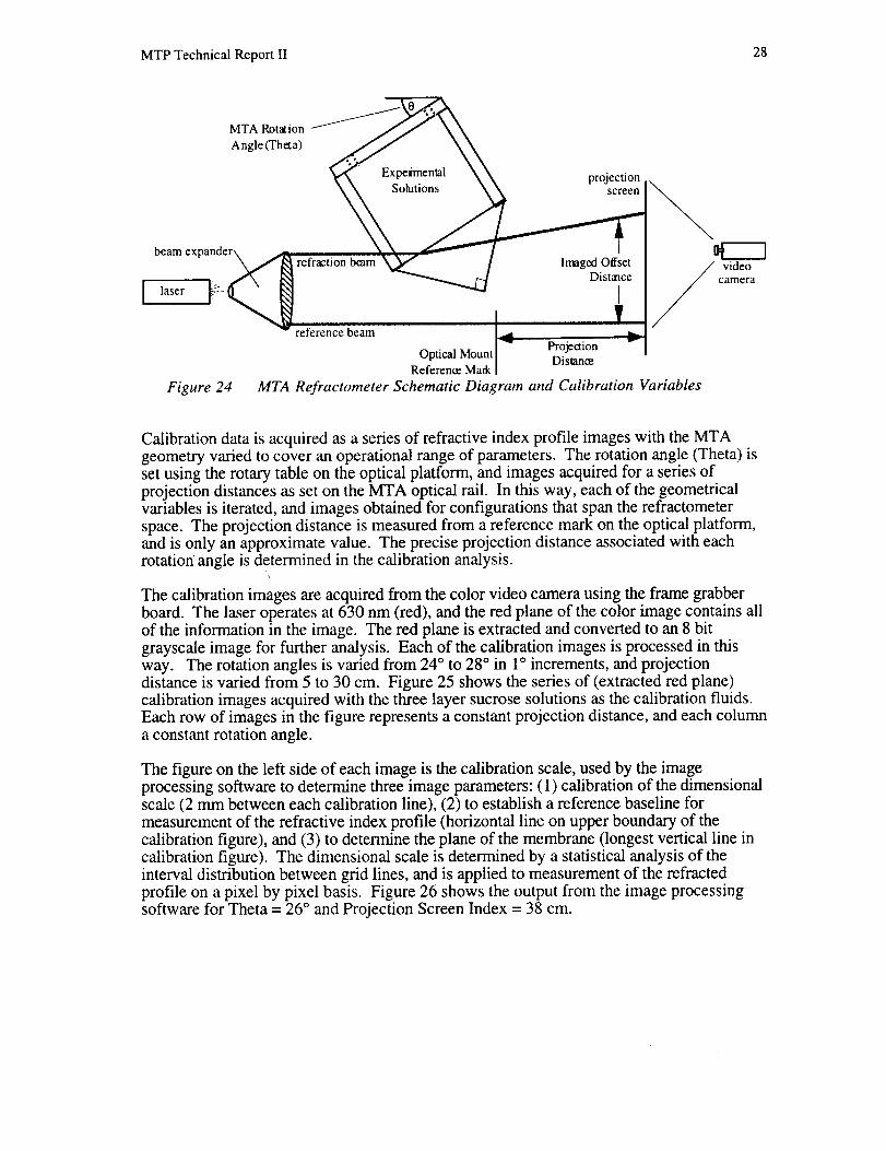
refractometer geometry's. There are the two primary variables in the refractometergeometry: (1) MTA Rotation Angle (Theta) and (2) Projection Distance. Theta defines thelaser beam incidence angle relative to the fluid cell, and the projection distance is a measureof the distance the refracted beam travels to the projection screen. Figure 24 shows aschematic of the MTA refractometer, and how these two variables affect the optical
geometry.
MTP Technical Report II 28
MTA Rotation __
Angle (Thet a) __,,,,,,,,,_, _
_S_tio":" \ \ projection
beam expander\ _7, \ x_ _L..,J,---- / I
. _,f _ refraction beam ____......._ J IrnagedDisOtffs_te
laserreference beam I-_
ReOPfieC_nI MMaUnnkt Pl_is°'_OiOn
Figure 24
video
camera
MTA Refractometer Schematic Diagram and Calibration Variables
Calibration data is acquired as a series of refractive index profile images with the MTAgeometry varied to cover an operational range of parameters. The rotation angle (Theta) isset using the rotary table on the optical platform, and images acquired for a series ofprojection distances as set on the MTA optical rail. In this way, each of the geometricalvariables is iterated, and images obtained for configurations that span the refractometerspace. The projection distance is measured from a reference mark on the optical platform,and is only an approximate value. The precise projection distance associated with eachrotation angle is determined in the calibration analysis.
The calibration images are acquired from the color video camera using the frame grabber
board. The laser operates at 630 nm (red), and the red plane of the color image contains allof the information in the image. The red plane is extracted and converted to an 8 bit
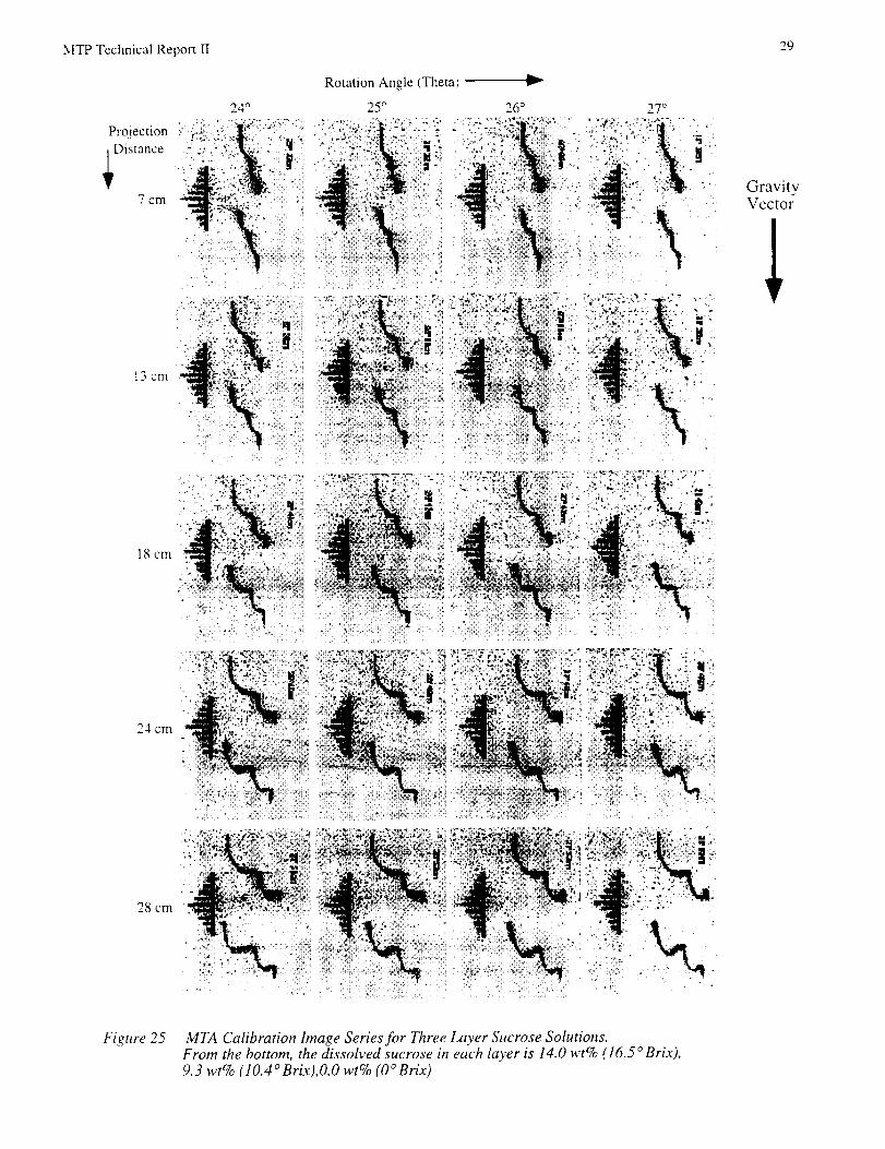
grayscale image for further analysis. Each of the calibration images is processed in thisway. The rotation angles is varied from 24 ° to 28 ° in 1° increments, and projectiondistance is varied from 5 to 30 cm. Figure 25 shows the series of (extracted red plane)
calibration images acquired with the three layer sucrose solutions as the calibration fluids.Each row of images in the figure represents a constant projection distance, and each column
a constant rotation angle.
The figure on the left side of each image is the calibration scale, used by the image
processing software to determine three image parameters: (1) calibration of the dimensionalscale (2 nun between each calibration line), (2) to establish a reference baseline for
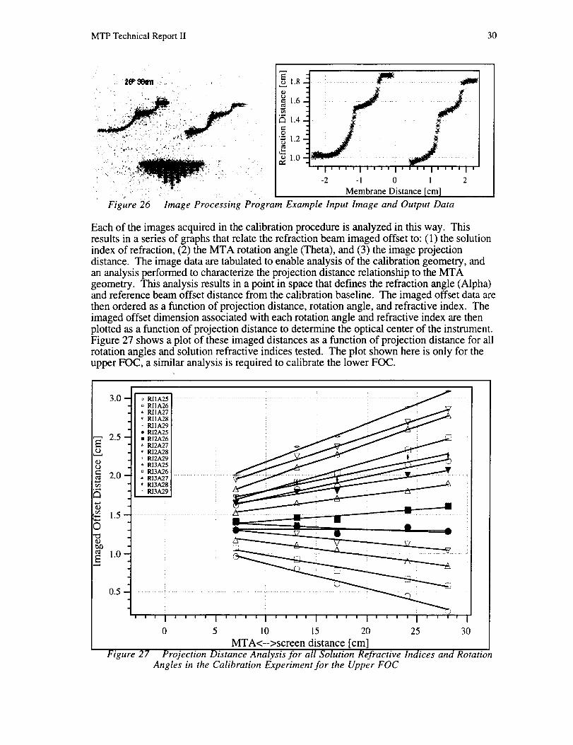
measurement of the refractive index profile (horizontal line on upper boundary of thecalibration figure), and (3) to determine the plane of the membrane (longest vertical line incalibration figure). The dimensional scale is determined by a statistical analysis of theinterval distribution between grid lines, and is applied to measurement of the refractedprofile on a pixel by pixel basis. Figure 26 shows the output from the image processingsoftware for Theta = 26 ° and Projection Screen Index = 38 cm.
MTP Technical Report II 29
Projection .,
Distance
7 cm
24 °
13 cm
24 cm
Rotation Angle (Theta)
25 °
V
GravityVector
28 cm
Figure 25 MTA Calibration Image Series for Three Layer Sucrose Solutions.From the bottom, the dissolved sucrose in each layer is 14.0 wt% (16.5 ° Brix),9.3 wt% ( l O.4° Brix),O.O wt% (O° Brix)
MTP Technical Report II 30
2EP_o'fl
Figure 26
1.8 .....
I_ 1.6_
1.41
!
-2
Jj" !i
.... i .... I .... I .... /'
-1 0 1 2
Membrane Distance [cm]
Image Processing Program Example Input Image and Output Data
Each of the images acquired in the calibration procedure is analyzed in this way. Thisresults in a series of graphs that relate the refraction beam imaged offset to: (1) the solutionindex of refraction, (2) the MTA rotation angle (Theta), and (3) the image projectiondistance. The image data are tabulated to enable analysis of the calibration geometry, andan analysis performed to characterize the projection distance relationship to the MTAgeometry. This analysis results in a point in space that defines the refraction angle (Alpha)and reference beam offset distance from the calibration baseline. The imaged offset data arethen ordered as a function of projection distance, rotation angle, and refractive index. Theimaged offset dimension associated with each rotation angle and refractive index are thenplotted as a function of projection distance to determine the optical center of the instrument.Figure 27 shows a plot of these imaged distances as a function of projection distance for allrotation angles and solution refractive indices tested. The plot shown here is only for theupper FOC, a similar analysis is required to calibrate the lower FOC.
"1 _ RIIA26 I _"r _2 i3.0 --t o RIIA25I - ............. .................. : !q • RIIA27 I /" i
..J " RI1A28 [ / _,.,,,,_,,,_/r-_. :
.J - RIIA29 ] ./- ../'_f,'_
• RI2A25 . i .... i _
• RI2A28
.o-t ............................ .....
= 1.5 ........ i ........ ....... _................. ! ........ --i ..........
....... I .... I .... I .... I .... I ' ' ' I
0 5 10 15 20 25 30
MTA<-->screen distance [cm]Figure 27 Projection Distance Analysis for all Solution Refractive Indices and Rotation
Angles in the Calibration Experiment for the Upper FOC
MTP Technical Report II 31
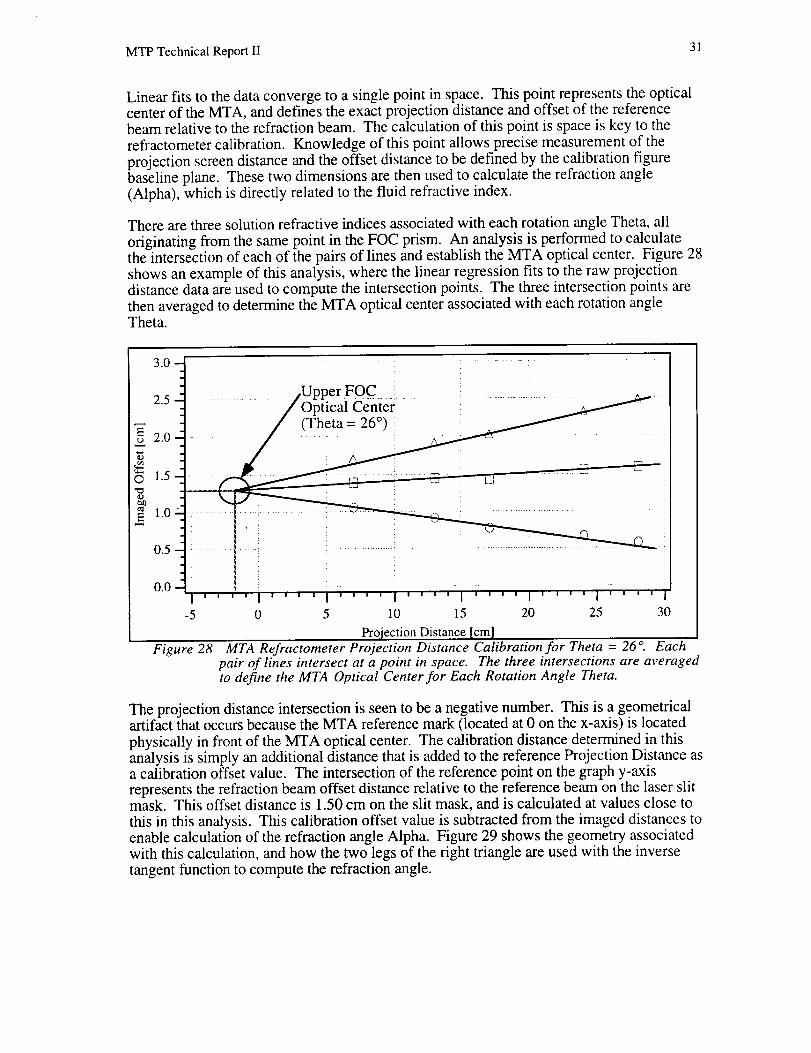
Linear fits to the data converge to a single point in space. This point represents the opticalcenter of the MTA, and defines the exact projection distance and offset of the referencebeam relative to the refraction beam. The calculation of this point is space is key to the
refractometer calibration. Knowledge of this point allows precise measurement of the
projection screen distance and the offset distance to be defined by the calibration figurebaseline plane. These two dimensions are then used to calculate the refraction angle
(Alpha), which is directly related to the fluid refractive index.
There are three solution refractive indices associated with each rotation angle Theta, all
originating from the same point in the FOC prism. An analysis is performed to calculatethe intersection of each of the pairs of lines and establish the MTA optical center. Figure 28shows an example of this analysis, where the linear regression fits to the raw projectiondistance data are used to compute the intersection points. The three intersection points are
then averaged to determine the MTA optical center associated with each rotation angleTheta.
3.0
2.5
2.0
1.5
1.0
0.5
0.0!
/UPtPeriFOCter ......... i j,.,--'''_
...............................................................
' I I I, , i I ' ' i , I I I I I I I I I I I | I I I I I I I I I
-5 0 5 I0 15 20 25 30
Projection Distance [cm]MTA Refractometer Projection Distance Calibration for Theta = 26 o. Each
pair of lines intersect at a point in space. The three intersections are averagedto define the MTA Optical Center for Each Rotation Angle Theta.
Figure 28
The projection distance intersection is seen to be a negative number. This is a geometricalartifact that occurs because the MTA reference mark (located at 0 on the x-axis) is located
physically in front of the MTA optical center. The calibration distance determined in thisanalysis is simply an additional distance that is added to the reference Projection Distance asa calibration offset value. The intersection of the reference point on the graph y-axis
represents the refraction beam offset distance relative to the reference beam on the laser slitmask. This offset distance is 1.50 cm on the slit mask, and is calculated at values close to
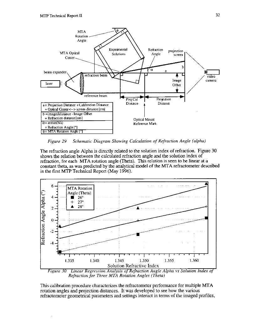
this in this analysis. This calibration offset value is subtracted from the imaged distances toenable calculation of the refraction angle Alpha. Figure 29 shows the geometry associatedwith this calculation, and how the two legs of the right triangle are used with the inverse
tangent function to compute the refraction angle.
MTP Technical Report II 32
MTA __
Re tionMTA Optizal I\\ Solutions XX projection
beam expander_ _
reference oeam
°LProjection
a= Projection Dist_ace +Calibration Distance Distmce Distanoe
= Optical Center<--> screen distance [cm]
b =i magedd istance - Image Offset
= Refraction distance [cm] Optical Mountc¢=araan(b/a) Reference Mark
= Refraction Angle [°]0 = MTA Rotaion Angle [°]
video
camera
Figure 29 Schematic Diagram Showing Calculation 03"Refraction Angle (alpha)
The refraction angle Alpha is directly related to the solution index of refraction. Figure 30shows the relation between the calculated refraction angle and the solution index of
refraction, for each MTA rotation angle (Theta). This relation is seen to be linear at a
constant theta, as was predicted by the analytical model of the MTA refractometer described
in the first MTP Technical Report (May 1996).
%,
e"O
°,.._
e3
6MTA Rotation
]Angle (Thoeta)41-- ] • 26 ............... _ "
....I: x:: ........... ,............. _,0
-2, ..... "*" ....
-4
Figure 30
' I .... I .... I .... I .... I .... I ' '
1.335 1.340 1.345 1.350 1.355 1.360
Solution Refractive Index
Linear Regression Analysis of Refraction Angle Alpha vs Solution Index ofRefraction for Three MTA Rotation Angles (Theta)
This calibration procedure characterizes the refractometer performance for multiple MTArotation angles and projection distances. It was developed to see how the variousrefractometer geometrical parameters and settings interact in terms of the imaged profiles,
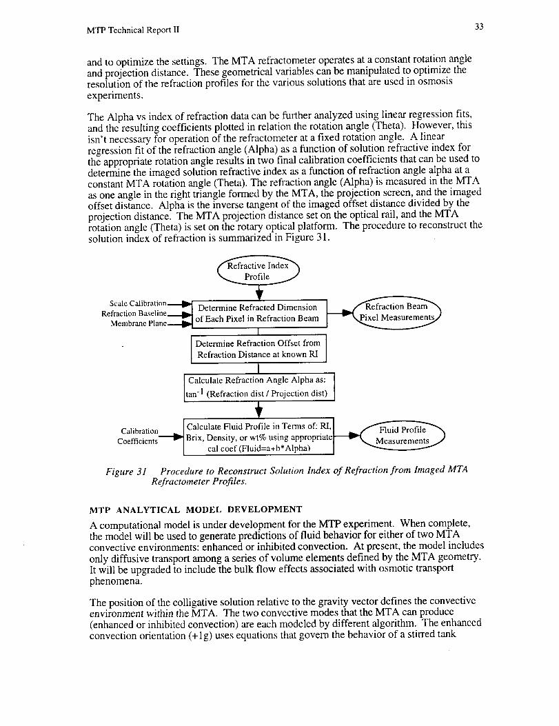
MTP Technical Report II 33
and to optimize the settings. The MTA refractometer operates at a constant rotation angle
and projection distance. These geometrical variables can be manipulated to optimize theresolution of the refraction profiles for the various solutions that are used in osmosis
experiments.
The Alpha vs index of refraction data can be further analyzed using linear regression fits,and the resulting coefficients plotted in relation the rotation angle (Theta). However, thisisn't necessary for operation of the refractometer at a fixed rotation angle. A linear
regression fit of the refraction angle (Alpha) as a function of solution refractive index forthe appropriate rotation angle results in two final calibration coefficients that can be used todetermine the imaged solution refractive index as a function of refraction angle alpha at aconstant MTA rotation angle (Theta). The refraction angle (Alpha) is measured in the MTAas one angle in the right triangle formed by the MTA, the projection screen, and the imagedoffset distance. Alpha is the inverse tangent of the imaged offset distance divided by theprojection distance. The MTA projection distance set on the optical rail, and the MTArotation angle (Theta) is set on the rotary optical platform. The procedure to reconstruct thesolution index of refraction is summarized in Figure 31.
Scale Calibration-......._Refraction Baseline........_ Determine Refracted Dimension
Membrane Plane--.--_ of Each Pixel in Refraction BeamI
Determine Refraction Offset fromRefraction Distance at known RI
I
I Calculate Refraction Angle Alpha as: Itan-1 (Refraction dist ! Projection dist)
___ Calculate Fluid Profile in Terms of: RI, I _._ _Calibration Brix, Density, or wt% using appropriater-""l_ Measurements j)
Coefficients cal coef (Fluid=a+b*Alpha) I
Figure 31 Procedure to Reconstruct Solution Index of Refraction from Imaged MTARefractometer Profiles.
MTP ANALYTICAL MODEL DEVELOPMENT
A computational model is under development for the MTP experiment. When complete,the model will be used to generate predictions of fluid behavior for either of two MTAconvective environments: enhanced or inhibited convection. At present, the model includes
only diffusive transport among a series of volume elements defined by the MTA geometry.It will be upgraded to include the bulk flow effects associated with osmotic transport
phenomena.
The position of the colligative solution relative to the gravity vector defines the convectiveenvironment within the MTA. The two convective modes that the MTA can produce
(enhanced or inhibited convection) are each modeled by different algorithm. The enhancedconvection orientation (+lg) uses equations that govern the behavior of a stirred tank
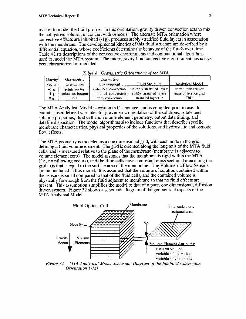
MTP Technical Report II 34
reactor to model the fluid profile. In this orientation, gravity driven convection acts to mixthe colligative solution in concert with osmosis. The alternate MTA orientation whereconvective effects are inhibited (-1 g), produces stably stratified fluid layers in associationwith the membrane. The developmental kinetics of this fluid structure are described by a
differential equation, whose coefficients determine the behavior of the fluids over time.Table 4 lists descriptions of the convective environments and computational algorithmsused to model the MTA system. The microgravity fluid convective environment has not yetbeen characterized or modeled.
Table 4 Gravimetric Orientations of the MTA
Gravity Gravimetric ConvectiveVector Orientation Environment
+1 g solute on top enhanced convection-1 g solute on bottom inhibited convection0 g n/a zero convection
Fluid Structure
unstably stratified layersstably stratified layers
stratified layers ?
Analvtical Model
stirred tank reactor
finite difference gridTBD
The MTA Analytical Model is written in C language, and is compiled prior to use. Itcontains user defined variables for gravimetric orientation of the solutions, solute andsolution properties, fluid cell and volume element geometry, output data timing, anddatafile disposition. The model algorithms also include functions that describe specificmembrane characteristics, physical properties of the solutions, and hydrostatic and osmoticflow effects.
The MTA geometry is modeled as a one dimensional grid, with each node in the griddefining a fluid volume element. The grid is oriented along the long axis of the MTA fluidcells, and is measured relative to the plane of the membrane (membrane is adjacent tovolumeelement zero). The model assumes that the membrane is rigid within the MTA
(i.e., no pillowing occurs), and the fluid cells have a constant cross sectional area along thegrid axis that is equal to the surface area of the membrane. The Volumetric Flow Sensorsare not included in this model. It is assumed that the volume of solution contained within
the sensors is small compared to that of the fluid cells, and the contained volume isphysically far enough from the fluid adjacent to membrane so that no fluid effects arepresent. This assumption simplifies the model to that of a pure, one dimensional, diffusiondriven system. Figure 32 shows a schematic diagram of the geometrical aspects of theMTA Analytical Model.
Fluid Optical Cell internode cross
sectional area
Vol_ro¢ l_lement Attributes:-constant volume
-variable solute moles
-variable solvent moles
MTA Analytical Model Schematic Diagram in the Inhibited ConvectionOrientation (-l g)
Gravity ] Volume
Vector_ Elements
Figure 32
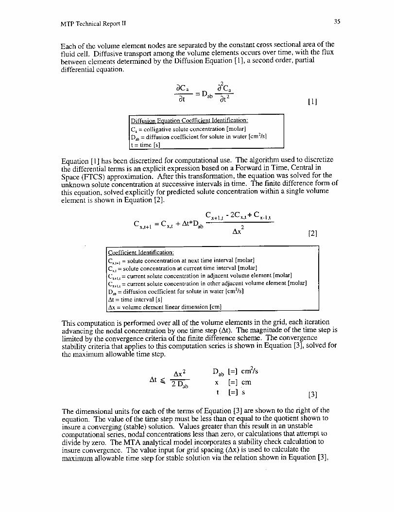
MTP Technical Report II 35
Each of the volume element nodes are separated by the constant cross sectional area of the
fluid cell. Diffusive transport among the volume elements occurs over time, with the fluxbetween elements determined by the Diffusion Equation [ 1], a second order, partial
differential equation.
_C a _2C a
_t = Dab _t 2[1]
Diffusion Equation Coefficient Identification:
Ca = colligative solute concentration [molar]Dab = diffusion coefficient for solute in water [cm2/s]
t = time Is]
Equation [1] has been discretized for computational use. The algorithm used to discretizethe differential terms is an explicit expression based on a Forward in Time, Central in
Space (FTCS) approximation. After this transformation, the equation was solved for theunknown solute concentration at successive intervals in time. The finite difference form of
this equation, solved explicitly for predicted solute concentration within a single volume
element is shown in Equation [2].
Cx,t+ 1 = Cx, t + At*Dab
Cx+l, t - 2Cx,t+ Cx.1, t
Ax 2[2]
Coefficient Identification:
Cx,t÷ 1 ._. solute concentration at next time interval [molar]
C_,_= solute concentration at current time interval [molar]
Cx+_.t= current solute concentration in adjacent volume element [molar]
Cx+_,t= current solute concentration in other adjacent volume element [molar]Dab= diffusion coefficient for solute in water [cmZ/s]
At = time interval [s]
Ax = volume element linear dimension [cm]
This computation is performed over all of the volume elements in the grid, each iterationadvancing the nodal concentration by one time step (At). The magnitude of the time step islimited by the convergence criteria of the finite difference scheme. The convergencestability criteria that applies to this computation series is shown in Equation [3], solved forthe maximum allowable time step.
AX 2 Dab [=] cm2/s
At <_ 2 Dab X [=] cm
t [=] s [3]
The dimensional units for each of the terms of Equation [3] are shown to the right of theequation. The value of the time step must be less than or equal to the quotient shown toinsure a converging (stable) solution. Values greater than this result in an unstablecomputational series, nodal concentrations less than zero, or calculations that attempt todivide by zero. The MTA analytical model incorporates a stability check calculation toinsure convergence. The value input for grid spacing (Ax) is used to calculate themaximum allowable time step for stable solution via the relation shown in Equation [3],
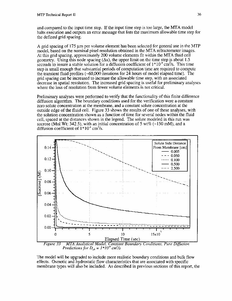
MTP Technical Report II 36
and compared to the input time step. If the input time step is too large, the MTA modelhalts execution and outputs an error message that lists the maximum allowable time step for
the defined grid spacing.
A grid spacing of 175 gm per volume element has been selected for general use in the MTPmodel, based on the nominal pixel resolution obtained in the MTA refractometer images.At this grid spacing, approximately 200 volume elements fit within the MTA fluid cellgeometry. Using this node spacing (Ax), the upper limit on the time step is about 1.5seconds to insure a stable solution for a diffusion coefficient of 1* 10.4 cm2/s. This time
step is small enough that substantial periods of computation time are required to computethe transient fluid profiles (-60,000 iterations for 24 hours of model elapsed time). Thegrid spacing can be increased to increase the allowable time step, with an associateddecrease in spatial resolution. The increased grid spacing is useful for preliminary analyseswhere the loss of resolution from fewer volume elements is not critical.
Preliminary analyses were performed to verify that the functionality of this finite differencediffusion algorithm. The boundary conditions used for the verification were a constantzero solute concentration at the membrane, and a constant solute concentration at the
outside edge of the fluid cell. Figure 33 shows the results of one of these analyses, withthe solution concentration shown as a function of time for several nodes within the fluid
cell, spaced at the distances shown in the legend. The solute modeled in this run wassucrose (Mol Wt: 342.5), with an initial concentration of 5 wt% (-150 mM), and adiffusion coefficient of 1* 10 .4 cmZ/s.
0.1,i
0.12
0.04
0.02
0.00
0
Figure 33
Solute Side Distance
From Membrane [cm]0.005
--- 0.050..... 0.100--- 0.500..... 2.500
35 10 15x10
Elapsed Time (sec)MTA Analytical Model, Constant Boundary Conditions, Pure Diffusion
Predictions for D,b = 1 *10" cm2/s
The model will be upgraded to include more realistic boundary conditions and bulk floweffects. Osmotic and hydrostatic flow characteristics that are associated with specificmembrane types will also be included. As described in previous sections of this report, the
MTP Technical Report II 37
Volumetric Flow Sensors (VFS) have provided data for trans-membrane flow rates as a
function of hydrostatic pressure (AP) and osmotic chemical potential (Ala). These flowcharacteristics will be fit to polynomial equations using data obtained from the MTA
experiments. The polynomials will then be used as empirical relations to define themembrane boundary condition (grid element 0) for each computational time interval. The
driving force for osmosis is then defined by the colligative solute concentration in thevolume element adjacent to the membrane.
DC-9 MICROGRAVITY EXPERIMENT DEVELOPMENT
Two experiments are planned for the MTP DC-9 microgravity flights: (1) testing the FluidManipulation System (FMS) to transfer fluids within various test cell geometry's, and (2)Refractometer Verification Experiment (RVE) for the observation of fluid refractive index
under microgravity conditions. The two experiments are run separately, and shareequipment within the MTP experiment rack. The microgravity flights are currentlyscheduled for the week of 16 December 1996. A MTP Safety and Engineering Document
was generated and submitted to NASA in preparation for the flights. This documentdescribes the experiment in detail and lists several engineering analyses required for flight.
Fluid Manipulation System (FMS) ExperimentTwo candidate MTP Fluid Optical Cell (FOC) geometry's have been developed for this
experiment: (1) Quarter Circle cell and (2) Triangular cell. These test cells each have adifferent internal geometry, and will be tested to assess the completeness of filling and
draining, and the propensity to trap air bubbles or leave fluid behind during fluidmanipulation procedures in microgravity. The cells are sized to allow completefilling/draining within the -20 seconds of microgravity afforded by each parabolic dive.During the course of performing these experiments, it is anticipated that incomplete fillingor draining will occur in some instances. In this event, a small interval of time (<30seconds) is required to reset the fluid cells to an initial condition in preparation for the nextdive.
The filling/draining operations will be conducted in each of the candidate fluid cells for aseries of fluid pumping rates and filling schemes, one scenario per parabolic dive. Foreach scenario, one dive will be used to fill the fluid cell, and the subsequent dive used toassess the draining operation under the same experimental conditions. Thus, a minimum of
two parabolic dives is required for each fluid manipulation condition. Repeat experimentswill be conducted at successful pumping rates as flight conditions allow.
Colored, deionized water is used in all FMS experiments to visualize the fluid flow
patterns. The two MTA computer controlled peristaltic pumps are used to automaticallymanipulate the fluids during microgravity, with each experiment initiated by a single mouseclick at the onset of a parabolic dive. A Video Cassette Recorder (VCR) will acquire imagedata showing the completeness of filling/draining. The video system includes a character
generator that is interfaced to the computer to allow real time display of elapsed time and g-level data directly over the fluid cell images during filling operations.
Refractometer Verification Experiment (RVE)The second experiment for the MTP microgravity flights involves verification of opticalrefractometer performance. These tests involve the visualization of fluid refractive index asa function of gravity level for a variety of fluids using a small (hand held) refractometer thatis secured to the experiment rack. The fluids used in these experiments are all non-hazardous aqueous solutions. Prior to a parabolic dive, a small quantity (-3 drops) of thetest solution is placed onto the refractometer sensing element using a liquid dropper (in l-g). The fluid is contained on the refractometer sensing element by a plastic cover, so no
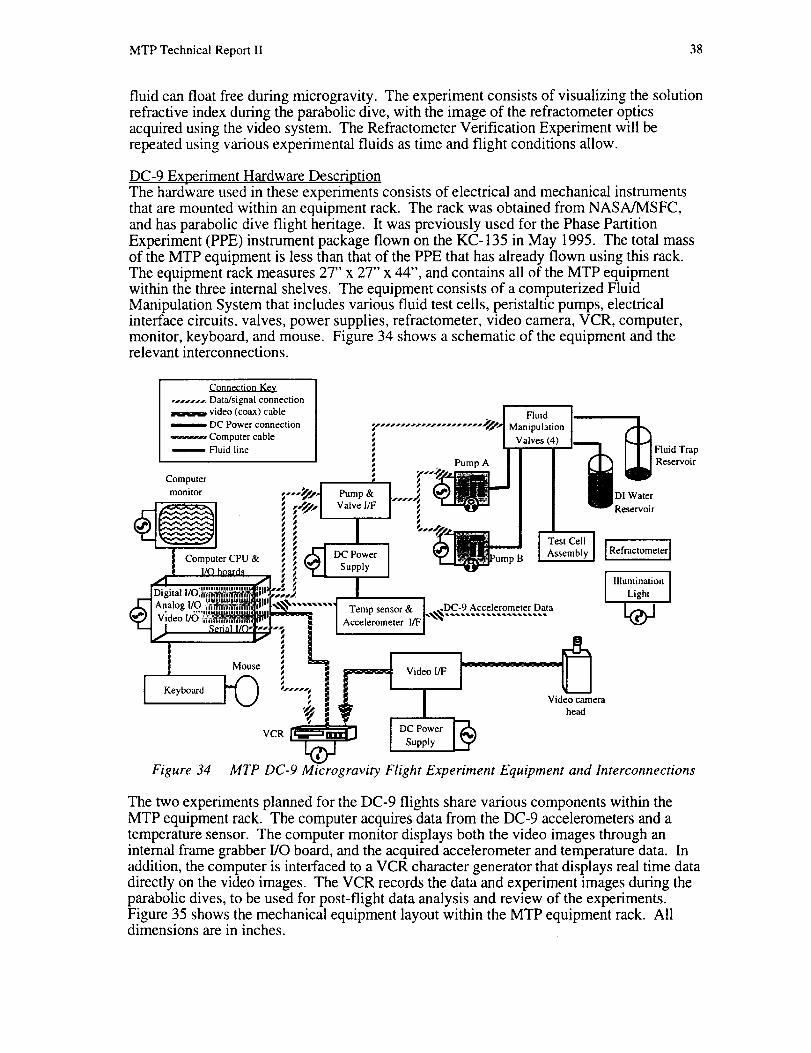
MTP Technical Report II 38
fluid can float free during microgravity. The experiment consists of visualizing the solutionrefractive index during the parabolic dive, with the image of the refractometer opticsacquired using the video system. The Refractometer Verification Experiment will berepeated using various experimental fluids as time and flight conditions allow.
DC-9 Experiment Hardware DescriptionThe hardware used in these experiments consists of electrical and mechanical instrumentsthat are mounted within an equipment rack. The rack was obtained from NASA/MSFC,and has parabolic dive flight heritage. It was previously used for the Phase Partition
Experiment (PPE) instrument package flown on the KC-135 in May 1995. The total massof the MTP equipment is less than that of the PPE that has already flown using this rack.The equipment rack measures 27" x 27" x 44", and contains all of the MTP equipmentwithin the three internal shelves. The equipment consists of a computerized FluidManipulation System that includes various fluid test cells, peristaltic pumps, electricalinterface circuits, valves, power supplies, refractometer, video camera, VCR, computer,monitor, keyboard, and mouse. Figure 34 shows a schematic of the equipment and therelevant interconnections.
Connection Key
...... D ta/ig 1 ti_._,- a S na connec on
video (coax) cable
DC Power connection
Computer cable
Fluid line
Computer
• / n°id I.................... _ Manipulation I
/ Valves(4)I__,.,_.; I I .!.. I I IwuidTrap
, PumpA | I (| "_ I | IReservoir
mp,, 1.... I iD'Wa,erValvel_ I ,' _ I _R_ervoi,
I '..--e..,_ II .,,__ I Test Cell I i i
DCPower om I"s emI"YI ISappl>'I i ,,lumioa,,o,,I
I Light I
mo.itor _""_'l
!.,,.#.,, I i
t J ",,.# _ | ,JL I Videocamera" _ , ] head
VCR _ I , I 1'l_,,,')• _n I DC Power
I SuppJy
Figure 34 MTP DC-9 Microgravity Flight Experiment Equipment and lnterconnections
The two experiments planned for the DC-9 flights share various components within the
MTP equipment rack. The computer acquires data from the DC-9 accelerometers and atemperature sensor. The computer monitor displays both the video images through aninternal frame grabber I/O board, and the acquired accelerometer and temperature data. Inaddition, the computer is interfaced to a VCR character generator that displays real time datadirectly on the video images. The VCR records the data and experiment images during theparabolic dives, to be used for post-flight data analysis and review of the experiments.Figure 35 shows the mechanical equipment layout within the MTP equipment rack. Alldimensions are in inches.
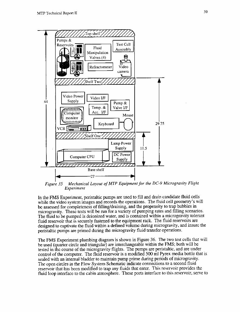
MTP Technical Report II 39
44
LFigure 35
Pumps &
__Reservoirs I
_ i
Test Cell
AssemblyFluid
Manipulation
Valves (4) Vide_o] Refractometer]
ca__]
Shelf Two
Video Power
SupplyVideo I/F [ [ _ump_ ]
I Temp'& [ ValveI/FAcc.I/F
_ Mouse
Base27 shelf
29.75
Mechanical Layout of MTP Equipment for the DC-9 Microgravity Flight
Experiment
In the FMS Experiment, peristaltic pumps are used to fill and drain candidate fluid cellswhile the video system images and records the operations. The fluid cell geometry's willbe assessed for completeness of filling/draining, and the propensity to trap bubbles inmicrogravity. These tests will be run for a variety of pumping rates and filling scenarios.The fluid to be pumped is deionized water, and is contained within a microgravity tolerantfluid reservoir that is securely fastened to the equipment rack. The fluid reservoirs aredesigned to captivate the fluid within a defined volume during microgravity, and insure theperistaltic pumps are primed during the microgravity fluid transfer operations.
The FMS Experiment plumbing diagram is shown in Figure 36. The two test cells that willbe used (quarter circle and triangular) are interchangeable within the FMS; both will betested in the course of the microgravity flights. The pumps are peristaltic, and are undercontrol of the computer. The fluid reservoir is a modified 500 ml Pyrex media bottle that issealed with an internal bladder to maintain pump prime during periods of microgravity.
The open circles in the Flow System Schematic indicate connections to a second fluidreservoir that has been modified to trap any fluids that enter. This reservoir provides thefluid loop interface to the cabin atmosphere. These ports interface to this reservoir, serve to
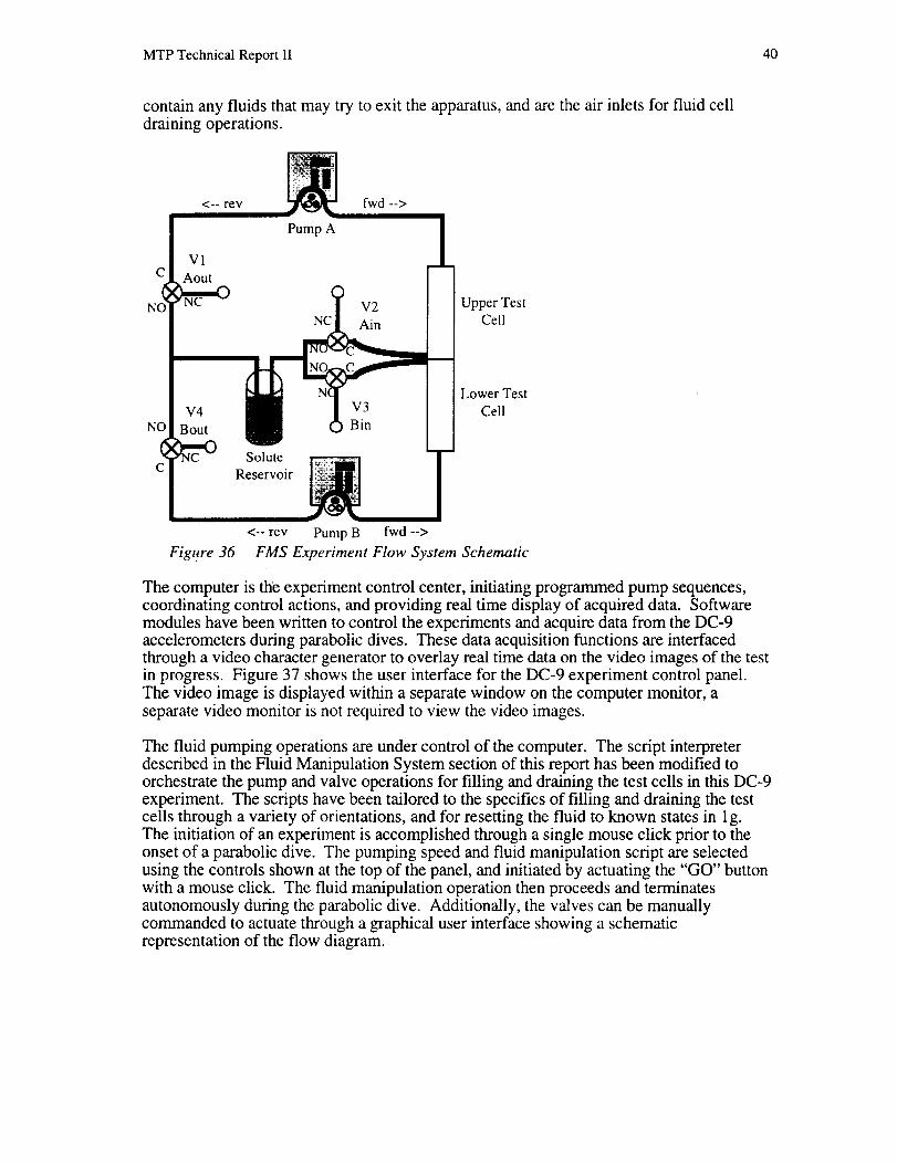
MTP Technical Report II 40
contain any fluids that may try to exit the apparatus, and are the air inlets for fluid cell
draining operations.
cV1
Aout
Pump A
NC
V4 V3
NO Bout Bin
CSolute
Reservoir
V2
Ain
Upper TestCell
Lower Test
Cell
<-- rev Pump B fwd -->
Figure 36 FMS Experiment Flow System Schematic
The computer is tlae experiment control center, initiating programmed pump sequences,coordinating control actions, and providing real time display of acquired data. Softwaremodules have been written to control the experiments and acquire data from the DC-9accelerometers during parabolic dives. These data acquisition functions are interfacedthrough a video character generator to overlay real time data on the video images of the testin progress. Figure 37 shows the user interface for the DC-9 experiment control panel.
The video image is displayed within a separate window on the computer monitor, aseparate video monitor is not required to view the video images.
The fluid pumping operations are under control of the computer. The script interpreterdescribed in the Fluid Manipulation System section of this report has been modified toorchestrate the pump and valve operations for filling and draining the test cells in this DC-9experiment. The scripts have been tailored to the specifics of filling and draining the testcells through a variety of orientations, and for resetting the fluid to known states in 1g.The initiation of an experiment is accomplished through a single mouse click prior to theonset of a parabolic dive. The pumping speed and fluid manipulation script are selectedusing the controls shown at the top of the panel, and initiated by actuating the "GO" buttonwith a mouse click. The fluid manipulation operation then proceeds and terminatesautonomously during the parabolic dive. Additionally, the valves can be manuallycommanded to actuate through a graphical user interface showing a schematicrepresentation of the flow diagram.
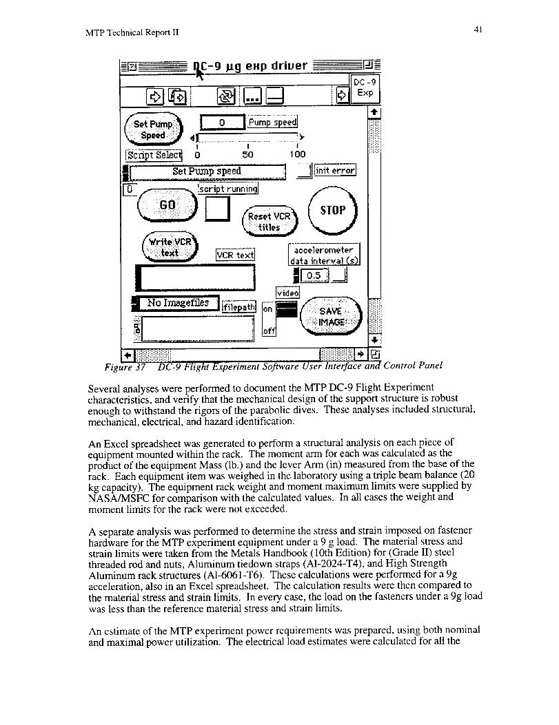
MTP Technical Report II 41
IVCRtextl
|..No I ,gef s t
accelerometer ]data interval(s)I
III
!¢iili:!i!i!!
, l!iiiiiiiilUiiii l!ii!iU!!!i!iil*Figure 37 DC-9 Flight Experiment Software User Interface and Control Panel
Several analyses were performed to document the MTP DC-9 Flight Experimentcharacteristics, and verify that the mechanical design of the support structure is robust
enough to withstand the rigors of the parabolic dives. These analyses included structural,mechanical, electrical, and hazard identification.
An Excel spreadsheet was generated to perform a structural analysis on each piece ofequipment mounted within the rack. The moment arm for each was calculated as theproduct of the equipment Mass (lb.) and the lever Arm (in) measured from the base of therack. Each equipment item was weighed in the laboratory using a triple beam balance (20kg capacity). The equipment rack weight and moment maximum limits were supplied byNASA/MSFC for comparison with the calculated values. In all cases the weight andmoment limits for the rack were not exceeded.
A separate analysis was performed to determine the stress and strain imposed on fastenerhardware for the MTP experiment equipment under a 9 g load. The material stress andstrain limits were taken from the Metals Handbook (10th Edition) for (Grade II) steel
threaded rod and nuts, Aluminum tiedown straps (AI-2024-T4), and High StrengthAluminum rack structures (AI-606 l-T6). These calculations were performed for a 9gacceleration, also in an Excel spreadsheet. The calculation results were then compared tothe material stress and strain limits. In every case, the load on the fasteners under a 9g loadwas less than the reference material stress and strain limits.
An estimate of the MTP experiment power requirements was prepared, using both nominaland maximal power utilization. The electrical load estimates were calculated for all the
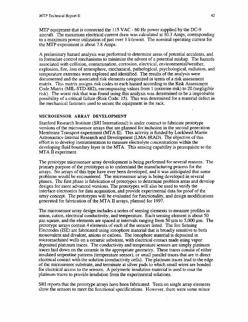
MTP Technical Report II 42
MTP equipment that is connected the 115 VAC - 60 Hz power supplied by the DC-9aircraft. The maximum electrical current draw was calculated at 10.3 Amps, correspondingto a maximum power utilization of just over 1 kilowatt. The nominal operating current forthe MTP experiment is about 7.8 Amps.
A preliminary hazard analysis was performed to determine areas of potential accidents, andto formulate control mechanisms to minimize the advent of a potential mishap. The hazardsassociated with collision, contamination, corrosion, electrical, environmental/weather,
explosion, fire, loss of atmosphere, mechanical, pathological, psychological, radiation, andtemperature extremes were explored and identified. The results of the analysis weredocumented and the associated risk elements categorized in terms of a risk assessmentmatrix. This matrix assigns risk codes to each hazard according to the Risk AssessmentCode Matrix (MIL-STD-882), encompassing values from 1 (extreme risk) to 20 (negligiblerisk). The worst risk that was found using this analysis was determined to be a improbablepossibility of a critical failure (Risk Code: 15). This was determined for a material defect inthe mechanical fasteners used to secure the equipment in the rack.
MICROSENSOR ARRAY DEVELOPMENT
Stanford Research Institute (SRI International) is under contract to fabricate prototypeversions of the microsensor arrays that are planned for inclusion in the second generationMembrane Transport experiment (MTA ID. This activity is funded by Lockheed MartinAstronautics-Internal Research and Development (LMA-IRAD). The objective of thiseffort is to develop instrumentation to measure electrolyte concentrations within thedeveloping fluid boundary layer in the MTA. This sensing capability is prerequisite to theMTA I1 experiment.
The prototype microsensor array development is being performed for several reasons. Theprimary purpose of the prototypes is to understand the manufacturing process for thearrays. No arrays of this type have ever been developed, and it was anticipated that someproblems would be encountered. The microsensor array is being developed in severalphases. The first phase is fabrication of prototypes to determine problem areas and developdesigns for more advanced versions. The prototypes will also be used to verify theinterface electronics for data acquisition, and provide experimental data for proof of thearray concept. The prototypes will be evaluated for functionality, and design modificationsgenerated for fabrication of the MTA II arrays, planned for 1997.
The microsensor array design includes a series of sensing elements to measure profiles inanion, cation, electrical conductivity, and temperature. Each sensing element is about 50p.m square, and the elements are spaced at intervals ranging from 50 p.m to 5,000 p.m. Theprototype arrays contain 4 elements of each of the sensors listed. The Ion Sensing
Electrodes (ISE) are fabricated using ionophore material that is broadly sensitive to bothmonovalent and divalent, anions or cations. The ionophore material is deposited inmicromachined wells on a ceramic substrate, with electrical contact made using vapordeposited platinum traces. The conductivity and temperature sensors are simply platinumtraces laid down on the ceramic in the appropriate geometry. These traces consist of eitherinsulated serpentine patterns (temperature sensor), or small parallel traces that are in directelectrical contact with the solution (conductivity cells). The platinum traces lead to the edgeof the microsensor substrate, and terminate at silver pads to which small wires are bondedfor electrical access to the sensors. A polymeric insulation material is used to coat theplatinum traces to provide insulation from the experimental solutions.
SRI reports that the prototype arrays have been fabricated. Tests on single array elementsshow the sensors to meet the functional specifications. However, there were some minor
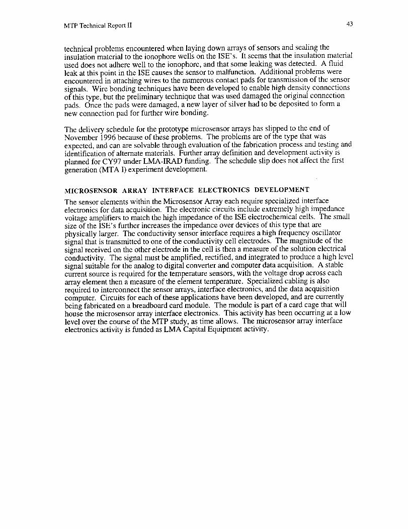
MTP Technical Report II 43
technical problems encountered when laying down arrays of sensors and sealing theinsulation material to the ionophore wells on the ISE's. It seems that the insulation materialused does not adhere well to the ionophore, and that some leaking was detected. A fluid
leak at this point in the ISE causes the sensor to malfunction. Additional problems wereencountered in attaching wires to the numerous contact pads for transmission of the sensorsignals. Wire bonding techniques have been developed to enable high density connectionsof this type, but the preliminary technique that was used damaged the original connection
pads. Once the pads were damaged, a new layer of silver had to be deposited to form anew connection pad for further wire bonding.
The delivery schedule for the prototype microsensor arrays has slipped to the end ofNovember 1996 because of these problems. The problems are of the type that wasexpected, and can are solvable through evaluation of the fabrication process and testing andidentification of alternate materials. Further array definition and development activity is
planned for CY97 under LMA-IRAD funding. The schedule slip does not affect the firstgeneration (MTA I) experiment development.
MICROSENSOR ARRAY INTERFACE ELECTRONICS DEVELOPMENT
The sensor elements within the Microsensor Array each require specialized interface
electronics for data acquisition. The electronic circuits include extremely high impedancevoltage amplifiers to match the high impedance of the ISE electrochemical cells. The smallsize of the ISE's further increases the impedance over devices of this type that are
physically larger. The conductivity sensor interface requires a high frequency oscillatorsignal that is transmitted to one of the conductivity cell electrodes. The magnitude of thesignal received on the other electrode in the cell is then a measure of the solution electricalconductivity. The signal must be amplified, rectified, and integrated to produce a high levelsignal suitable for the analog to digital converter and computer data acquisition. A stablecurrent source is required for the temperature sensors, with the voltage drop across eacharray element then a measure of the element temperature. Specialized cabling is alsorequired to interconnect the sensor arrays, interface electronics, and the data acquisitioncomputer. Circuits for each of these applications have been developed, and are currentlybeing fabricated on a breadboard card module. The module is part of a card cage that willhouse the microsensor array interface electronics. This activity has been occurring at a lowlevel over the course of the MTP study, as time allows. The microsensor array interface
electronics activity is funded as LMA Capital Equipment activity.