MEM01: DC-Motor ServomechanismInterdisciplinary Automatic Controls Laboratory - ME/ECE/CHE 389

February 5, 2016

Contents

1 Introduction and Goals 1

2 Description 2

3 Modeling 2

4 Lab Objective 5

5 Model Identification 55.1 Model Identification: Open-loop Step Response Analysis . . . . . . . . . . . . . . . . . . 55.2 Model Identification: Open-loop Frequency Response Analysis . . . . . . . . . . . . . . . 7

6 Velocity Controller Design 8

7 Position Controller Design 8

1 Introduction and Goals

The Precision Modular Servo (PMS) workshop serves as a model of a very popular device, the DC ServoMotor. This is often used in robotic applications. The word ‘servo’ comes from the Latin word servusmeaning servant or slave. Thus the servo motor is intended to react to a given command, for examplea desired position or velocity. In order for the motor to be called a servo motor it has to be equippedwith a velocity and position measurement unit and motor driver. It may also include a simple servo motorcontroller. The main features distinguishing servo motors from normal motors are:

• minimized rotor inertia,

• minimized armature inductance,

• improved withstand voltage and magnet saturation,

• designed to withstand sudden acceleration and high frequency operation.

The PMS unit allows for the design of different servo motor controllers and to test them in real time usingthe Matlab and Simulink environment.

1

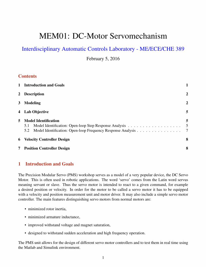
Figure 1: Precision Modular Servo mechanical unit

2 Description

The description of the PMS setup in this section refers mostly to the mechanical part and the controlaspect. For details of the mechanical and electrical connection, the interface and an explanation of howthe signals are measured and transferred to the PC, refer to the “Installation & Commissioning” manual.As shown in Figure 1, the PMS mechanical unit consists of a DC Motor, Tachometer/Gearbox, DigitalEncoder, Input and Output Potentiometers and Magnetic Brake.

Apart from the mechanical units, the electrical units play an important role for motor control. They allowmeasured signals to be transferred to the PC via an I/O card. The amplifiers are used to transfer controlsignals from the PC to the DC Motor. The mechanical and electrical units provide a complete controlsystem setup presented in Figure 2.

In order to design any control algorithms one must first understand the physical background behind theprocess and carry out identification experiments. The next section explains the modelling process of thePMS.

3 Modeling

Every control project starts with plant modeling, so as much information as possible is given about theprocess itself. The mechanical-electrical model of the servo motor is presented in Figure 3. For the DCmotor model, nonlinearities are so small that they can be neglected. According to the electrical-mechanicaldiagram presented in Figure 3 the linear model equations can be derived.

2

Figure 2: PMS control system

The torque τ generated by the DC motor is proportional to the motor current i:

τ = Kti, (1)

where Kt is the torque constant. The induced electromotive force, vemf , is a voltage proportional to theangular shaft velocity θ:

vemf = Kbθ, (2)

where Kb s a motor property dependant constant related to physical properties of the motor. Using New-tons law the mechanical dynamics can be described by:

Jθ =∑

τi = −dθ +Kti, (3)

where d is a linear approximation of the viscous friction. The equations governing the behaviour of theelectrical model are:

u− vemf = Ldi

dt+Ri, (4)

where u is the control signal. Including equation (2) transforms (4) into:

u = Ldi

dt+Ri+Kbθ. (5)

Q1: Use equations (3) and (5) to write the motor model in state space form by defining the state vector ax = [ω i]T , were ω = θ represents the angular velocity, and the output as y = ω.

Q2: Give an expression for the transfer function G(s) = Y (s)/U(s). What is the order of the transferfunction? What are the units of the input and the output?

Table 1 gives the values of the motor parameters supplied by the manufacturer. The motor used forthe experiments is a 24V DC brushed motor with a no-load speed of 4050 rpm. An extra gain termka = 24/2.5 = 9.6 needs to be added to input of the model to represent the gain provided by the PA150Preamplifier and SA150 Servo Amplifier. In this way, the model can be run with a 2.5 V control signal

3

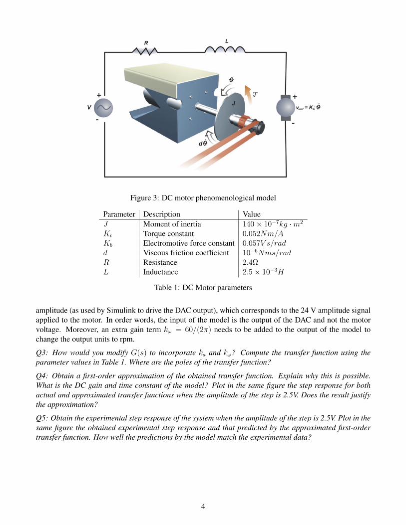
Figure 3: DC motor phenomenological model

Parameter Description ValueJ Moment of inertia 140× 10−7kg ·m2

Kt Torque constant 0.052Nm/AKb Electromotive force constant 0.057V s/radd Viscous friction coefficient 10−6Nms/radR Resistance 2.4ΩL Inductance 2.5× 10−3H

Table 1: DC Motor parameters

amplitude (as used by Simulink to drive the DAC output), which corresponds to the 24 V amplitude signalapplied to the motor. In order words, the input of the model is the output of the DAC and not the motorvoltage. Moreover, an extra gain term kω = 60/(2π) needs to be added to the output of the model tochange the output units to rpm.

Q3: How would you modify G(s) to incorporate ka and kω? Compute the transfer function using theparameter values in Table 1. Where are the poles of the transfer function?

Q4: Obtain a first-order approximation of the obtained transfer function. Explain why this is possible.What is the DC gain and time constant of the model? Plot in the same figure the step response for bothactual and approximated transfer functions when the amplitude of the step is 2.5V. Does the result justifythe approximation?

Q5: Obtain the experimental step response of the system when the amplitude of the step is 2.5V. Plot in thesame figure the obtained experimental step response and that predicted by the approximated first-ordertransfer function. How well the predictions by the model match the experimental data?

4

4 Lab Objective

In this laboratory you will obtain a experimentally validated model for the DC motor-based servomech-anism and design model-based controllers to regulate both the speed and the position of the servo. Aplant transfer function, i.e. the open loop response of the system, will be obtained from experimental data.Identification of model parameters from experimental data is known as system identification.

5 Model Identification

In this section, you will obtain the plant transfer function (open loop system) by two separate system iden-tification methods: i) analysis of the open loop step response and ii) analysis of the open loop frequencyresponse.

5.1 Model Identification: Open-loop Step Response Analysis

Assume the plant G(s) is of the form

G(s) =k

τs+ 1, (6)

i.e. a first order linear system with a stable (LHP) pole. The objective of system identification is todetermine the steady state gain k and the time constant τ from experimental data. If the system, G(s), isexcited by a step input of magnitude A, the response will be

U(s) =A

s, Y (s) = G(s)U(s) =

Ak

s(τs+ 1). (7)

Then, the steady-state value yss of y(t) can be computed by the the final value theorem, i.e.,

yss = limt→∞

y(t) = lims→0

sY (s) = Ak, (8)

and the steady-state gain of the system can be obtained as

k =yssA. (9)

Note that yss can be obtained directly from the experimentally step response of the system as shown inFigure 4 (left).

By computing the inverse Laplace transform of Y (s) in (7), we can write

y(t) = Ak(1− e−t/τ ) = yss(1− e−t/τ ). (10)

Therefore,y(t)− yss

yss= −e−t/τ ⇐⇒ ln

(yss − y(t)

yss

)= − t

τ, (11)

which implies that if we plot ln((yss−y(t)/yss) versus t as shown in Figure 4 (right), we can obtain−1/τ ,and therefore τ , just by computing the slope of the plotted line.

5

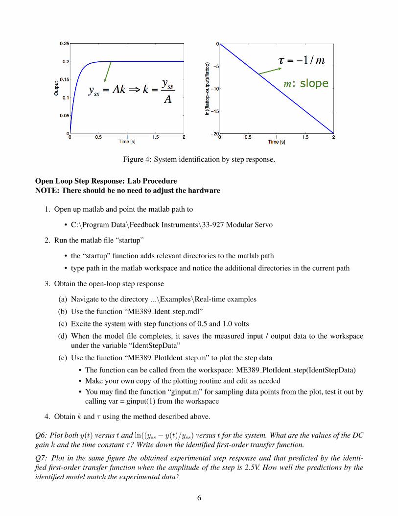
Figure 4: System identification by step response.

Open Loop Step Response: Lab ProcedureNOTE: There should be no need to adjust the hardware

1. Open up matlab and point the matlab path to

• C:\Program Data\Feedback Instruments\33-927 Modular Servo

2. Run the matlab file “startup”

• the “startup” function adds relevant directories to the matlab path

• type path in the matlab workspace and notice the additional directories in the current path

3. Obtain the open-loop step response

(a) Navigate to the directory ...\Examples\Real-time examples

(b) Use the function “ME389 Ident step.mdl”

(c) Excite the system with step functions of 0.5 and 1.0 volts

(d) When the model file completes, it saves the measured input / output data to the workspaceunder the variable “IdentStepData”

(e) Use the function “ME389 PlotIdent step.m” to plot the step data

• The function can be called from the workspace: ME389 PlotIdent step(IdentStepData)• Make your own copy of the plotting routine and edit as needed• You may find the function “ginput.m” for sampling data points from the plot, test it out by

calling var = ginput(1) from the workspace

4. Obtain k and τ using the method described above.

Q6: Plot both y(t) versus t and ln((yss − y(t)/yss) versus t for the system. What are the values of the DCgain k and the time constant τ? Write down the identified first-order transfer function.

Q7: Plot in the same figure the obtained experimental step response and that predicted by the identi-fied first-order transfer function when the amplitude of the step is 2.5V. How well the predictions by theidentified model match the experimental data?

6

5.2 Model Identification: Open-loop Frequency Response Analysis

For stable linear systems the open loop transfer function can be determined from the frequency response.The frequency response can be obtained from experimental data by exciting the system with a sinusoidalsignal of varying frequency. The measured gain and phase shift between the input and output signalconstitute the frequency response. The transfer function of the system can then be inferred from theexperimental Bode plot. For review of frequency response and bode plots see the lectures available on theweb.

Open Loop Frequency Response: Lab ProcedureNOTE: There should be no need to adjust the hardware

1. Excite the system with a sinusoidal function

(a) Use the function “ME389 Ident freq.mdl”(b) Connect the DAQ to the hardware

• Build the mdl file (compile the code), use the build button at the top left corner (Threearrows pointing down)

• Connect the DAQ to the hardware with the connect button• Power on the motor (green switch on the power supply)• When ready, run the mdl file with the green arrow

(c) Excite the system with a sinusoidal function of amplitude 0.5 Volts and frequency 2 rad/s(d) When the model file completes, it saves the measured input / output data to the workspace

under the variable “IdentFreqData”

2. Use the function “ME389 PlotIdent freq.m” to plot the input / output data

• The function can be called from the workspace: ME389 PlotIdent freq(IdentFreqData)• First the function plots the sampled data. Only the last 10 s are plotted since we are only

interested in steady state data.• The plot routine, then queries for a frequency, this is used as an initial guess to a fitting routine,

which will fit the measured data to a sinusoid of the form

Input : Ain sin (ωt+ φin) + offset and Output : Aout sin (ωt+ φout) + offset (12)

• The details of the fitting routing are not important.(a) However, it is sensitive to initial guess values(b) If you are not satisfied with the resulting fit, try again with a different frequency guess(c) Once you are satisfied with the fit, the plotting function will print the gain an phase shift,

which are determined from the fitted sinusoids

gain =Aout

Ainand Phase Shift = φout − φin (13)

3. Repeat the process for varying frequencies, with intervals of 5 per decade.

Q8: Plot the experimental Bode plot for the system. Write down the identified first-order transfer function.

Q9: Plot in the same figure the obtained experimental step response and that predicted by the identi-fied first-order transfer function when the amplitude of the step is 2.5V. How well the predictions by theidentified model match the experimental data?

7

Figure 5: Block diagram of servomechanism-based regulator.

6 Velocity Controller Design

Q10: Using the identified model of the plant obtained either in Section 5.1 or Section 5.2, compute the stepresponse of the open loop system for 0 <= t <= 2 using the Matlab command “step.” Use the Matlabcommand “stepinfo” to summarize the characteristics of the step response.

Q11: Consider a P controller (K(s)=Kp). Plot the position of the closed-loop poles as a function of thecontroller gain. Give an expression for the steady state error in the closed loop step response. Will thiscontroller guarantee zero steady-state error? How could you reduce the steady-state error? Could youdestabilize the closed-loop system by pursuing a smaller steady-state error? Could you drive the closed-loop system response into saturation by pursuing a smaller steady-state error. Compute the step responseof the closed-loop system for a “small” gain of Kp = 0.01 and for a “big” gain of Kp = 100. Plot boththe input and the output of the plant.

Q12: Consider a PI controller (K(s)=Kp+Ki/s). Give an expression for the steady state error in theclosed-loop step response. Will this controller guarantee zero steady-state error? Choose Kp and Ki suchthat the overshoot is less than 3% and the settling time is less than 0.5 s. Compute the step response ofthe closed-loop system for 0 <= t <= 4 using the Matlab command “step.” Use the Matlab command“stepinfo” to summarize the characteristics of the step response. Does the step response undershoot (goesbelow zero)? Explain why in the positive case. What can you do to eliminate the undershoot?

Q13: Test developed controller experimentally. Compare simulated (use ‘step’ command) and experimen-tal step responses. Compare simulated (use ’slim’ command) and experimental sinusoidal responses.

7 Position Controller Design

Q14: Using the identified model G(s) for the angular velocity in response to the voltage command, obtainthe model H(s) for the angular position in response to the same voltage command.

Q15: Using the identified model of the plant obtained either in Section 5.1 or Section 5.2, compute the stepresponse of the open loop system for 0 <= t <= 2 using the Matlab command “step.” Use the Matlabcommand “stepinfo” to summarize the characteristics of the step response.

Q16: Consider a P controller (K1(s) = Kp) with the structure shown in Figure 5 (Kd ≡ 0). Plot theposition of the closed-loop poles as a function of the controller gain. Give an expression for the steadystate error in the closed loop step response. Will this controller guarantee zero steady-state error? ObtainKp to guarantee an overshoot of 10%.

8

Q17: By root locus, show that you can improve performance by adding tachometer feedback (K2(s) = Kd)as proposed in Figure 5. Use the value of Kp obtained in the previous question. Improved performanceis evidenced by reduced overshoot without extending the risetime, or reduced risetime without incurringincreased overshoot. What value of Kd will allow you to demonstrate this improved performance?

Q18: Test developed controller experimentally. Compare simulated (use ‘step’ command) and experimen-tal step responses. Compare simulated (use ’slim’ command) and experimental sinusoidal responses.

9