MEM 255 Introduction to ControlSystems Introduction

Harry G. KwatnyDepartment of Mechanical Engineering & MechanicsDrexel University

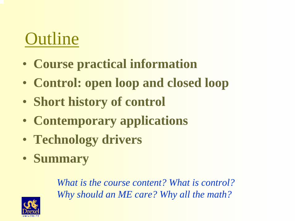
Outline• Course practical information• Control: open loop and closed loop• Short history of control• Contemporary applications• Technology drivers• Summary

What is the course content? What is control? Why should an ME care? Why all the math?

Practical Information• Lectures: Tues & Thurs 2-3:20 pm • Comp Lab: Fri only as announced, UG lab will be available at your

convenience except when a lab is in session• URL: http://www.pages.drexel.edu/faculty/hgk22.html• Text Book: G. F. Franklin, J. D. Powel, and A. Emami-Naeini, Feedback

Control of Dynamic Systems, 4th ed., Prentice Hall, 2002• Software: The MathWorks, Inc. The Student Edition of MATLAB, Version

6+Control Toolbox. (15 seats in UG laboratory). Tutorial @ http://www.engin.umich.edu/group/ctm/basic/basic.html

• TA: TBA• Grading:

Homework (3): 10%Midterm (in class): 30%Midterm Project (take home): 30%Final Project (take home): 30%

What you should know going in

• Linear ordinary differential equations,• Basics of Laplace transform,• How to model simple mechanical,

electrical, fluid and thermal systems.

MEM 255: What you should know going out• What is a linear system and why do ME’s care about them,• Concepts of state space and transfer function models of a

linear system.• How linear systems behave: input-output dynamics

The meaning of poles & zerosThe frequency transfer function and Bode Plots

• Block diagram manipulation• How linear systems behave: state dynamics

Eigenvalues & eigenvectors, modal analysis and similarity transformations.

• Stability and Routh table.• Basic ability to use MATLAB.

MEM355: What you should know going out• Understand why automatic control is useful for a

mechanical engineer• Recognize the value of integrated control and

process design• Understand the key concepts of control system

design• Be able to solve simple control problems• Recognize difficult control problems • Know relevant mathematical theory• Have competence in using computational tools

MEM 255: Specific Goals• Introduce time domain (state space) and transform domain (transfer function)

models of linear dynamical systems.• Develop the general process of deriving state pace models from physical

principles. • Introduce the methods of deriving transfer functions from state space models

and vice versa.• Introduce the basics of transform domain analysis: poles & zeros, the

frequency transfer function, Bode Plots and working with block diagrams.• Introduce the basics of time domain analysis: eigenvalues & eigenvectors,

state transition matrix and the “variation of parameters” formula, modal analysis and similarity transformations.

• Develop concept of stability and tools for parametric stability analysis.• Provide a comprehensive introduction to the control system computations

using MATLAB.

MEM 355: Specific Goals• Define the control system design problem and develop a preliminary

appreciation of the tradeoffs involved and requirements for robust stability and performance.

• Develop concepts and tools for ultimate state error analysis.• Develop the relationship between time domain and frequency domain

performance specifications, e.g, rise time, overshoot, settling time, sensitivity function and bandwidth.

• Develop frequency domain design methods, including: the root locus method, Nyquist & Bode methods, and stability margins.

• Provide an introduction to state space design: controllability and observability, pole placement, design via the separation principle (time permitting).

• Emphasize computational methods using MATLAB.

What is Control?• Control refers to the manipulation of the inputs to a

physical system in order to cause desirable behavior.Cause output variables to track desired valuesImpose desirable dynamical behavior, e.g., stabilize an unstablesystem

• Open loop (feedforward) controlExploit knowledge of system behavior to compute necessary inputsRequires accurate model of system

• Closed loop (feedback, active) controlProcess information from sensors to derive appropriate inputsAllows compensation for model uncertainty, disturbances, noiseAlters system dynamics

Open & Closed Loop Control

Feedforward does notalter plant dynamics. Feedback does.

Control computer

The Magic of Feedback• The adjustment of system inputs based on the observation of its outputs• Feedback is a universal strategy to cope with uncertainty

In engineering we use feedback:

• To cause a system to behave as desired

• To keep some variables constant

• To stabilize an unstable system

• To reduce effects of disturbances

• To minimize the effect of component variations

• As another alternative for designers

Origins of Control EngineeringClocks (escapement) 1200-1400Windmills 1787Steam Engines (Watt) 1788Maxwell ~ Governors 1868Water Turbines 1893Wright brothers ~ Airplane 1903Sperry ~ Autopilot (Gyro) 1914Minorsky ~ Ship steering 1922Black ~ Feedback amplifier 1928Ivanoff ~ Temperature regulation 1934

First real control system analysis.First journal article.Invention of new control paradigm.

Wilber Wright 1901

“We know how to construct airplanes. Men also know how to build engines. The inability to balance and steer still confronts students of the flying problem. When this one feature has been worked out, the age of flying will have arrived, for all other difficulties are of minor importance.”

•Power generation•Power transmission•Process control•Discrete manufacturing•Robotics•Communications•Automotive•Buildings •Aerospace

•Medicine•Marine Engineering•Computers•Instrumentation•Mechatronics•Materials•Physics•Biology•Economics

Contemporary ApplicationsWidespread use of automatic control in many fields

There is a unified framework of theory, design methods and computer tools that cut across fields of application.

Examples• Flight control systems

Commercial & military “fly-by-wire”Autopilot, auto-landingUAV

• RoboticsPrecision positioning in manufacturingRemote space/sea environmentsMinimally-invasive surgeryRPV’s for surveillance, search and rescue

• AutomotiveEngine TransmissionCruise, climate controlABS, Traction control, ESPActive suspension

• Power plantsVarious temps/pressuresPower outputEmissions control

• Heating, ventilation, air conditioning (HVAC)

Mercedes Benz SLR

Examples, Cont’d• Materials processing

Rapid thermal processingVapor deposition

• Noise and vibration control

Active mountsSpeaker systems

• Intelligent vehicle highway systems

‘platooning’ for high speed, high density travelAutomatic mergeObstacle avoidance

• Smart enginesCompression systems stall, surge, flutter controlCombustion systems lean air/fuel ratio for low emissions, improved efficiency

• Biology/BiomechanicsFeedback governs growth, response to stress,Feedback regulates body temperature, blood pressure, and cholesterol level,Feedback makes it possible to stand upright.Feedback enables locomotion.Feedback is pervasive: from the interaction of proteins in cells to the interaction of organisms in complex ecologies.

Active Control in AutomobilesA typical automobile has 200-300 feedback controllers. Here

are a few examples in a contemporary Mercedes.• Cruise Control• ABC-active body control• ABS-anti-lock braking system• ASR acceleration skid control• ESP electronic stabilization program• SBC sensotronic brake control• BAS brake assist system• Proximity controlled cruising

http://www.mercedes-benz.com/e/innovation/rd/sicherheitspecial/default.htm

Active Body Control•ABC continuously matches the stiffness and damping characteristics to current driving conditions.•It is possible, for example, to compensate for the rolling motion of the body when taking a bend in the road.•Hydraulic cylinders in series with the coil springs, generate forces that counteract wheel load. This is performed with sensors that measure yaw rate, longitudinal and transverse acceleration, vertical acceleration.

Key Technology Trends• Computation/microprocessors

Cheap and powerful microprocessors opened the door to widespread control applications from 1970’s onward

• Sensors and actuatorsSensors continue to get smaller, cheaper, fasterMacro/micro – scale actuation evolving (power electronics, piezo-electric, EM-rheological fluids)

• Communications and networkingNetworks replacing point-to-point communication in large systems (e.g., electric power systems) and small (e.g. automotive)

State Space & Transfer Function Models

( ) ( ) ( )( ) ( )( ) ( )

,

x Ax Bu x Fx Guy Cx Du y Hx Ju

Y s L y tY s G s U s

U s L u t

= + = += + = +

= ⎡ ⎤⎣ ⎦== ⎡ ⎤⎣ ⎦

East Coast NotationMATLAB

West Coast Notation

Transfer Function

State space models are also referred to as time-domain models

Transfer function models are alsoReferred to as frequency domain models.

Quarter-Car Suspension

1m

2m

1k

2k

1c

2c

r

( ) ( ) ( ) ( )( ) ( )

1 1 2 1 2 1 1 2 1 2 1 1

2 2 2 1 2 2 1 2

m x k x x k x r c x x c x r

m x k x x c x x

= − − − − − − − −

= − + −

Vertical motion, x1, x2 measured from rest withr=0

( ) ( )

( ) ( ) ( )

2

2 4 3 2

Using Laplace Transform, derive a relationshipbetween and (data from Franklin et al)

17.333/1.3067490 44067.5 157061 1.88099

R s X s

sX s R s

s s s s=

+ + + +

Quarter-Car State Space Model

( )( )

( )

( ) [ ]

1

11 11 2 1 2 2 2

1 11 21 11 1 1 1

1 12 2

2 22 2 2 22 1

2 2 2 21

1

1

2

2

0 1 0 0

0 0 0 1 0

0 0 1 0

cm

x xk k c c k c c kc cv vm m m md m m r tx xdtv vk c k c c c

m m m m m

xv

y txv

⎡ ⎤⎡ ⎤ ⎢ ⎥⎢ ⎥ ⎢ ⎥+⎡ ⎤ ⎡ ⎤+⎢ ⎥− − ⎢ ⎥⎢ ⎥ ⎢ ⎥ − + +⎢ ⎥ ⎢ ⎥⎢ ⎥ ⎢ ⎥= +⎢ ⎥ ⎢ ⎥⎢ ⎥ ⎢ ⎥⎢ ⎥ ⎢ ⎥⎢ ⎥ ⎢ ⎥⎢ ⎥ ⎢ ⎥⎣ ⎦ ⎣ ⎦− −⎢ ⎥ ⎢ ⎥⎢ ⎥⎣ ⎦ ⎢ ⎥⎣ ⎦

⎡ ⎤⎢ ⎥⎢ ⎥=⎢ ⎥⎢ ⎥⎣ ⎦

Evolution of the Control Discipline• Classical control 1940

Frequency-domain based tools for linear systemsMainly useful for single-input single-output (SISO) systemsWWII years saw 1st application of ‘optimal’ controlStill the main tools used in practice

• Modern control 1960‘State space’ approach for linear systemsUseful for SISO and multi-input multi-output (MIMO) systemsRelies on linear algebra computations rather than Laplace transformPerformance and robustness measures not always explicitJust in time for space exploration

• Optimal control 1970Find the input that optimizes some objective function (e.g., min fuel, min time)Used for both open loop and closed loop design

• Robust control 1980Generalizes classical control methods to MIMO caseEnabled by modern control development

• Nonlinear, adaptive, hybrid …

Research Applications in MEM• Automotive• Aircraft/Flight Safety• Power Plants• Robotics• Autonomous Vehicles• Mechatronics• Biology/Biomechanics• Electric Power Systems

Summary

• Course content. • What is a control system?

Open loop/closed loop (feedforward/feedback)• Why is control relevant to ME?

Applications! Applications! Applications!• Why so much math?

Abstraction to accommodate many applications in a common frameworkExplicit design approaches to meet (optimize) specific performance goals.