Mega-heatwave temperatures due to combined soil ... · 1 Supplementary Information Mega-heatwave temperatures due to combined soil desiccation and atmospheric heat buildup Diego G

1

Supplementary Information

Mega-heatwave temperatures due to combined soil desiccation and

atmospheric heat buildup

Diego G. Miralles1,2, Adriaan J. Teuling3, Chiel C. van Heerwaarden4 and Jordi Vilà-Guerau de

Arellano5

1 School of Geographical Sciences, University of Bristol, Bristol, BS81SS, United Kingdom

2 Laboratory of Hydrology and Water Management, Ghent University, B-9000 Ghent, Belgium

3 Hydrology and Quantitative Water Management Group, Wageningen University, 6709PA

Wageningen, The Netherlands

4 Max Planck Institute for Meteorology, 20146 Hamburg, Germany

5 Meteorology and Air Quality Section, Wageningen University, 6709PA Wageningen, The

Netherlands

Mega-heatwave temperatures due to combined soil desiccation and atmospheric heat accumulation

SUPPLEMENTARY INFORMATIONDOI: 10.1038/NGEO2141

NATURE GEOSCIENCE | www.nature.com/naturegeoscience 1

© 2014 Macmillan Publishers Limited. All rights reserved.

http://www.nature.com/doifinder/10.1038/ngeo2141

2

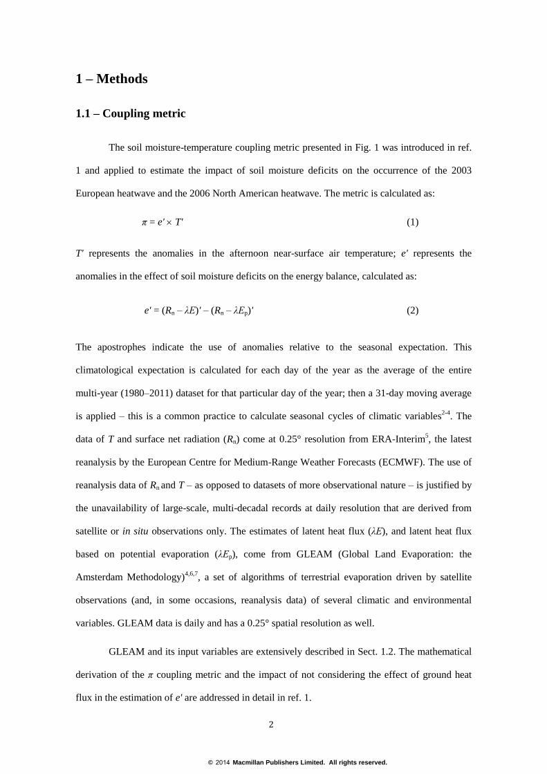
1 – Methods

1.1 – Coupling metric

The soil moisture-temperature coupling metric presented in Fig. 1 was introduced in ref.

1 and applied to estimate the impact of soil moisture deficits on the occurrence of the 2003

European heatwave and the 2006 North American heatwave. The metric is calculated as:

π = e' T' (1)

T' represents the anomalies in the afternoon near-surface air temperature; e' represents the

anomalies in the effect of soil moisture deficits on the energy balance, calculated as:

e' = (Rn – λE)' – (Rn – λEp)' (2)

The apostrophes indicate the use of anomalies relative to the seasonal expectation. This

climatological expectation is calculated for each day of the year as the average of the entire

multi-year (1980–2011) dataset for that particular day of the year; then a 31-day moving average

is applied – this is a common practice to calculate seasonal cycles of climatic variables2-4

. The

data of T and surface net radiation (Rn) come at 0.25° resolution from ERA-Interim5, the latest

reanalysis by the European Centre for Medium-Range Weather Forecasts (ECMWF). The use of

reanalysis data of Rn and T – as opposed to datasets of more observational nature – is justified by

the unavailability of large-scale, multi-decadal records at daily resolution that are derived from

satellite or in situ observations only. The estimates of latent heat flux (λE), and latent heat flux

based on potential evaporation (λEp), come from GLEAM (Global Land Evaporation: the

Amsterdam Methodology)4,6,7

, a set of algorithms of terrestrial evaporation driven by satellite

observations (and, in some occasions, reanalysis data) of several climatic and environmental

variables. GLEAM data is daily and has a 0.25° spatial resolution as well.

GLEAM and its input variables are extensively described in Sect. 1.2. The mathematical

derivation of the π coupling metric and the impact of not considering the effect of ground heat

flux in the estimation of e' are addressed in detail in ref. 1.


3

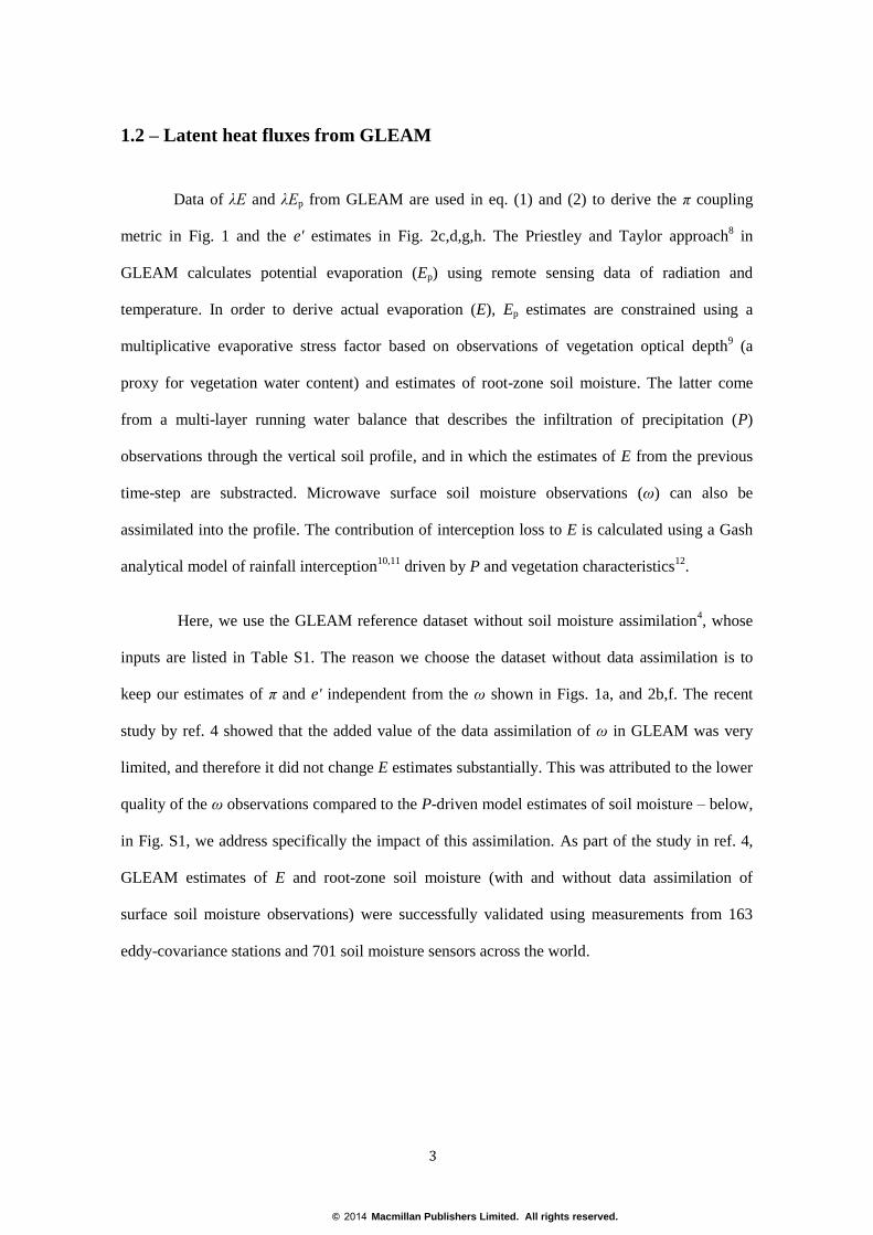
1.2 – Latent heat fluxes from GLEAM

Data of λE and λEp from GLEAM are used in eq. (1) and (2) to derive the π coupling

metric in Fig. 1 and the e' estimates in Fig. 2c,d,g,h. The Priestley and Taylor approach8 in

GLEAM calculates potential evaporation (Ep) using remote sensing data of radiation and

temperature. In order to derive actual evaporation (E), Ep estimates are constrained using a

multiplicative evaporative stress factor based on observations of vegetation optical depth9 (a

proxy for vegetation water content) and estimates of root-zone soil moisture. The latter come

from a multi-layer running water balance that describes the infiltration of precipitation (P)

observations through the vertical soil profile, and in which the estimates of E from the previous

time-step are substracted. Microwave surface soil moisture observations (ω) can also be

assimilated into the profile. The contribution of interception loss to E is calculated using a Gash

analytical model of rainfall interception10,11

driven by P and vegetation characteristics12

.

Here, we use the GLEAM reference dataset without soil moisture assimilation4, whose

inputs are listed in Table S1. The reason we choose the dataset without data assimilation is to

keep our estimates of π and e' independent from the ω shown in Figs. 1a, and 2b,f. The recent

study by ref. 4 showed that the added value of the data assimilation of ω in GLEAM was very

limited, and therefore it did not change E estimates substantially. This was attributed to the lower

quality of the ω observations compared to the P-driven model estimates of soil moisture – below,

in Fig. S1, we address specifically the impact of this assimilation. As part of the study in ref. 4,

GLEAM estimates of E and root-zone soil moisture (with and without data assimilation of

surface soil moisture observations) were successfully validated using measurements from 163

eddy-covariance stations and 701 soil moisture sensors across the world.


4

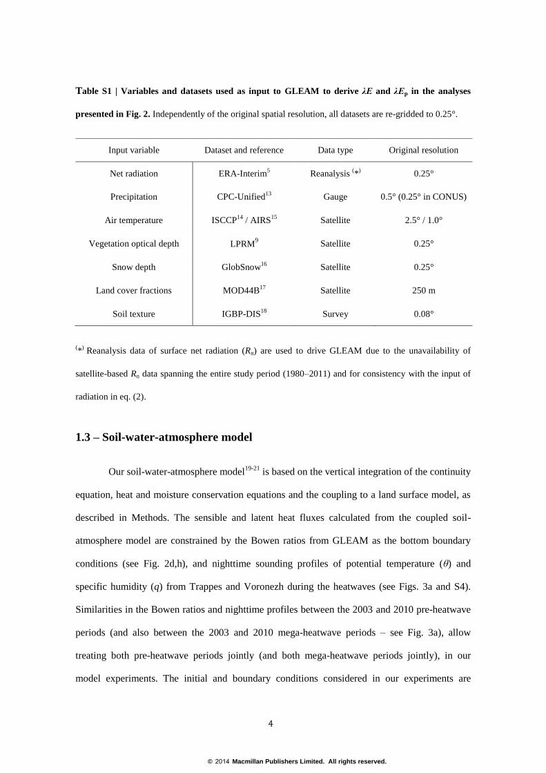
Table S1 | Variables and datasets used as input to GLEAM to derive λE and λEp in the analyses

presented in Fig. 2. Independently of the original spatial resolution, all datasets are re-gridded to 0.25°.

(*

) Reanalysis data of surface net radiation (Rn) are used to drive GLEAM due to the unavailability of

satellite-based Rn data spanning the entire study period (1980–2011) and for consistency with the input of

radiation in eq. (2).

1.3 – Soil-water-atmosphere model

Our soil-water-atmosphere model19-21

is based on the vertical integration of the continuity

equation, heat and moisture conservation equations and the coupling to a land surface model, as

described in Methods. The sensible and latent heat fluxes calculated from the coupled soil-

atmosphere model are constrained by the Bowen ratios from GLEAM as the bottom boundary

conditions (see Fig. 2d,h), and nighttime sounding profiles of potential temperature (θ) and

specific humidity (q) from Trappes and Voronezh during the heatwaves (see Figs. 3a and S4).

Similarities in the Bowen ratios and nighttime profiles between the 2003 and 2010 pre-heatwave

periods (and also between the 2003 and 2010 mega-heatwave periods – see Fig. 3a), allow

treating both pre-heatwave periods jointly (and both mega-heatwave periods jointly), in our

model experiments. The initial and boundary conditions considered in our experiments are

Input variable Dataset and reference Data type Original resolution

Net radiation ERA-Interim5 Reanalysis

(*

) 0.25°

Precipitation CPC-Unified13

Gauge 0.5° (0.25° in CONUS)

Air temperature ISCCP14

/ AIRS15

Satellite 2.5° / 1.0°

Vegetation optical depth LPRM9 Satellite 0.25°

Snow depth GlobSnow16

Satellite 0.25°

Land cover fractions MOD44B17

Satellite 250 m

Soil texture IGBP-DIS18

Survey 0.08°


5

summarized in Tables S2 and S3.

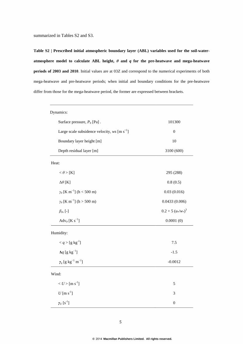
Table S2 | Prescribed initial atmospheric boundary layer (ABL) variables used for the soil-water-

atmosphere model to calculate ABL height, θ and q for the pre-heatwave and mega-heatwave

periods of 2003 and 2010. Initial values are at 03Z and correspond to the numerical experiments of both

mega-heatwave and pre-heatwave periods; when initial and boundary conditions for the pre-heatwave

differ from those for the mega-heatwave period, the former are expressed between brackets.

Dynamics:

Surface pressure, P0 [Pa] .

Large scale subsidence velocity, ws [m s−1

]

Boundary layer height [m]

Depth residual layer [m]

101300

0

10

3100 (600)

Heat:

< θ > [K]

Δθ [K]

γθ [K m−1

] (h < 500 m)

γθ [K m−1

] (h > 500 m)

βθv [-]

Advθ [K s−1

]

295 (288)

0.8 (0.5)

0.03 (0.016)

0.0433 (0.006)

0.2 + 5 (u*/w*)3

0.0001 (0)

Humidity:

< q > [g kg-1

]

Δq [g kg−1

]

γq [g kg−1

m−1

]

7.5

-1.5

-0.0012

Wind:

< U > [m s-1

]

U [m s-1

]

γU [s-1

]

5

3

0


6

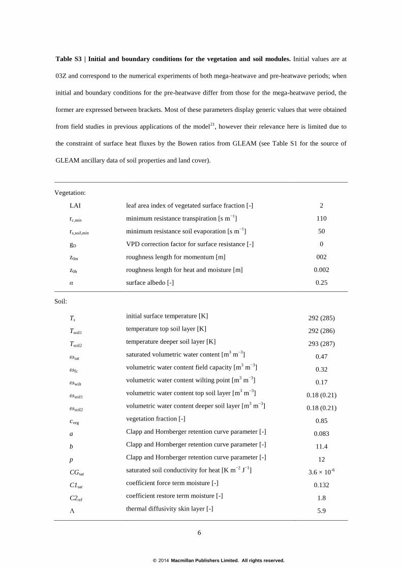
Table S3 | Initial and boundary conditions for the vegetation and soil modules. Initial values are at

03Z and correspond to the numerical experiments of both mega-heatwave and pre-heatwave periods; when

initial and boundary conditions for the pre-heatwave differ from those for the mega-heatwave period, the

former are expressed between brackets. Most of these parameters display generic values that were obtained

from field studies in previous applications of the model21

, however their relevance here is limited due to

the constraint of surface heat fluxes by the Bowen ratios from GLEAM (see Table S1 for the source of

GLEAM ancillary data of soil properties and land cover).

Vegetation:

LAI

rc,min

rs,soil,min

gD

z0m

z0h

α

leaf area index of vegetated surface fraction [-]

minimum resistance transpiration [s m−1

]

minimum resistance soil evaporation [s m−1

]

VPD correction factor for surface resistance [-]

roughness length for momentum [m]

roughness length for heat and moisture [m]

surface albedo [-]

2

110

50

0

002

0.002

0.25

Soil:

Ts

Tsoil1

Tsoil2

ωsat

ωfc

ωwilt

ωsoil1

ωsoil2

cveg

a

b

p

CGsat

C1sat

C2ref

Λ

initial surface temperature [K]

temperature top soil layer [K]

temperature deeper soil layer [K]

saturated volumetric water content [m3 m

−3]

volumetric water content field capacity [m3 m

−3]

volumetric water content wilting point [m3 m

−3]

volumetric water content top soil layer [m3 m

−3]

volumetric water content deeper soil layer [m3 m

−3]

vegetation fraction [-]

Clapp and Hornberger retention curve parameter [-]



saturated soil conductivity for heat [K m−2

J−1

]

coefficient force term moisture [-]

coefficient restore term moisture [-]

thermal diffusivity skin layer [-]

292 (285)

292 (286)

293 (287)

0.47

0.32

0.17

0.18 (0.21)

0.18 (0.21)

0.85

0.083

11.4

12

3.6 × 10-6

0.132

1.8

5.9


7

2 – Discussion

2.1 – Uncertainties in the large-scale coupling

Our results suggest that soil moisture deficits contributed to the 2003 and 2010 summer

heatwaves by intensifying air temperatures via direct and indirect mechanisms that were

mediated by the evolution of the ABL. Results in Fig. 2c,d show an anomalous contribution of

soil moisture deficits to soil heating (i.e. a large e') and how this coincides with the air

temperature anomalies (T') in the regions affected by the 2003 heatwave. Figure 2g,h show

analogous results for the 2010 event in Eastern Europe. Estimates of e' compare well to the

anomalies in surface soil moisture (ω') from the remote sensing product by ref. 22 (see Fig. 2b,f).

As mentioned in Sect. 2, the estimates of λE and λEp used to calculate e' in Fig. 2 (via eq. (2))

come from the GLEAM reference dataset without data assimilation of ω (see ref. 4 and Table

S1). This is done to make e' and ω' in Fig. 2 independent, which simplifies the straight

comparison between Fig. 2c,g and 2b,f and allows corroborating the dry-out from two separate

sources of information. Here, Fig. S1, reproduces the coupling results from Fig. 2 using the

version of GLEAM with data assimilation of ω. It can be observed that the patterns of e' remain

remarkably similar to those in Fig. 2, proving a small sensitivity of the GLEAM E estimates to

the assimilation routine as previously reported4 and discussed in Sect. 1.2.

The e' estimates shown in Fig. 2 are sensitive to the choice of GLEAM as methodology

for the derivation of λE and λEp. Analogous estimates of λE are available from the ERA-Interim

reanalysis, while λEp can also be derived based on radiation and temperature data from ERA-

Interim using a simple Priestley and Taylor8 formulation. Fig. S2 recreates the analyses in Fig.

2c,d,g,h using these ERA-Interim data only: T' is the ERA-Interim 2-meter afternoon temperature

(the same as in Fig. 2c,d,g,h), and e' is calculated using eq. (2) based on ERA-Interim data of Rn

(again as in Fig. 2c,d,g,h), ERA-Interim λE and λEp (derived via Priestley and Taylor with ERA-

Interim forcing). Note that, therefore, GLEAM is not used whatsoever in Fig. S2, and that this

figure is based on ERA-Interim reanalysis data only. Once again, the results compare well to


8

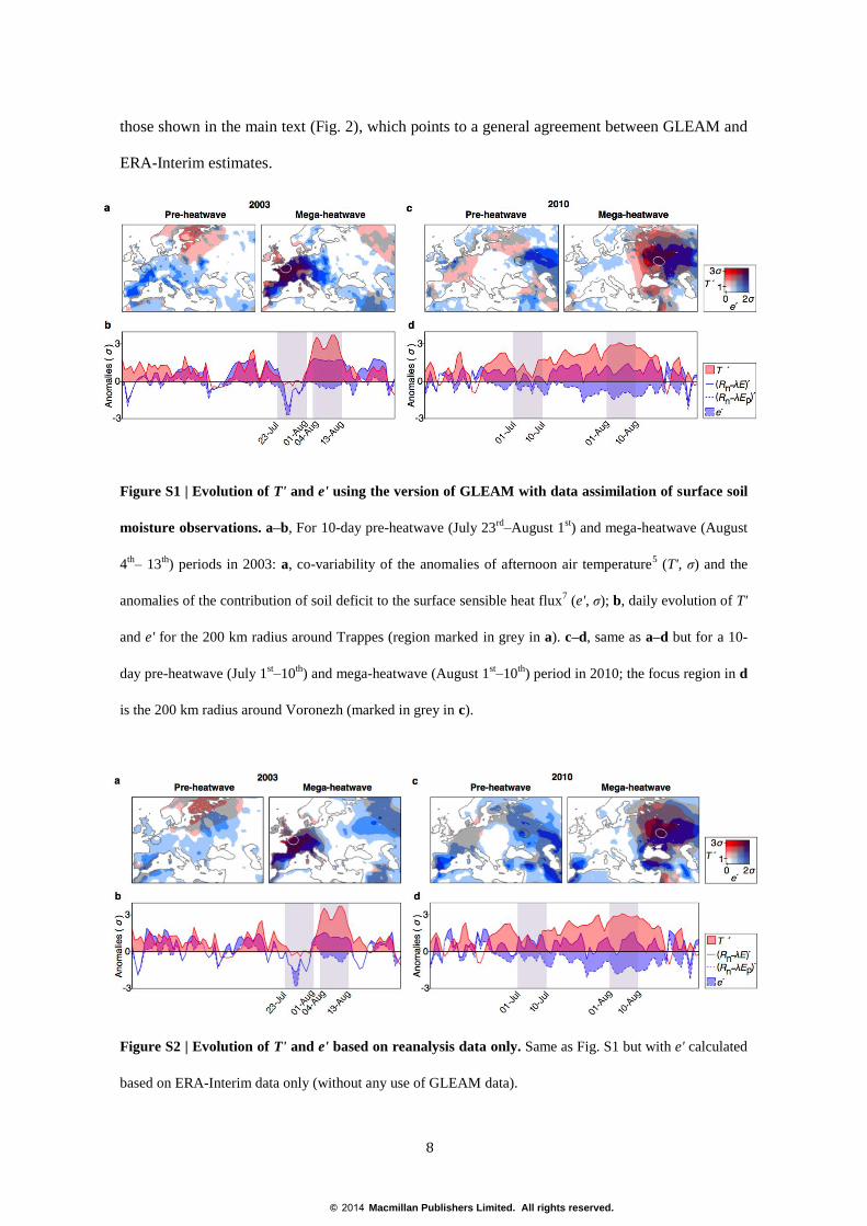
those shown in the main text (Fig. 2), which points to a general agreement between GLEAM and

ERA-Interim estimates.

Figure S1 | Evolution of T' and e' using the version of GLEAM with data assimilation of surface soil

moisture observations. a–b, For 10-day pre-heatwave (July 23rd–August 1

st) and mega-heatwave (August

4th– 13

th) periods in 2003: a, co-variability of the anomalies of afternoon air temperature

5 (T', σ) and the

anomalies of the contribution of soil deficit to the surface sensible heat flux7 (e', σ); b, daily evolution of T'

and e' for the 200 km radius around Trappes (region marked in grey in a). c–d, same as a–d but for a 10-

day pre-heatwave (July 1st–10

th) and mega-heatwave (August 1

st–10

th) period in 2010; the focus region in d

is the 200 km radius around Voronezh (marked in grey in c).

Figure S2 | Evolution of T' and e' based on reanalysis data only. Same as Fig. S1 but with e' calculated

based on ERA-Interim data only (without any use of GLEAM data).


9

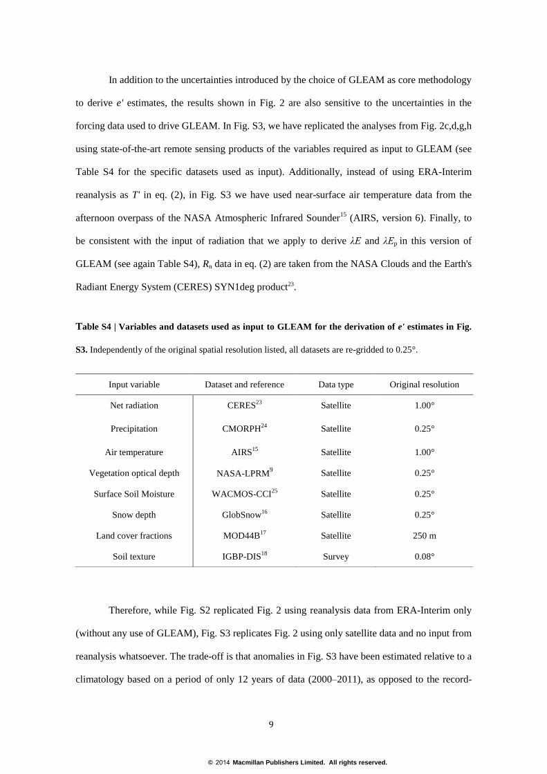
In addition to the uncertainties introduced by the choice of GLEAM as core methodology

to derive e' estimates, the results shown in Fig. 2 are also sensitive to the uncertainties in the

forcing data used to drive GLEAM. In Fig. S3, we have replicated the analyses from Fig. 2c,d,g,h

using state-of-the-art remote sensing products of the variables required as input to GLEAM (see

Table S4 for the specific datasets used as input). Additionally, instead of using ERA-Interim

reanalysis as T' in eq. (2), in Fig. S3 we have used near-surface air temperature data from the

afternoon overpass of the NASA Atmospheric Infrared Sounder15

(AIRS, version 6). Finally, to

be consistent with the input of radiation that we apply to derive λE and λEp in this version of

GLEAM (see again Table S4), Rn data in eq. (2) are taken from the NASA Clouds and the Earth's

Radiant Energy System (CERES) SYN1deg product23.

Table S4 | Variables and datasets used as input to GLEAM for the derivation of e' estimates in Fig.

S3. Independently of the original spatial resolution listed, all datasets are re-gridded to 0.25°.

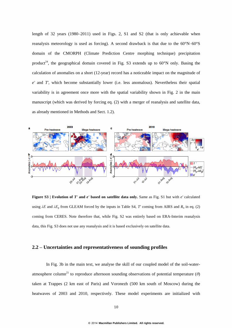
Therefore, while Fig. S2 replicated Fig. 2 using reanalysis data from ERA-Interim only

(without any use of GLEAM), Fig. S3 replicates Fig. 2 using only satellite data and no input from

reanalysis whatsoever. The trade-off is that anomalies in Fig. S3 have been estimated relative to a

climatology based on a period of only 12 years of data (2000–2011), as opposed to the record-

Input variable Dataset and reference Data type Original resolution

Net radiation CERES23

Satellite 1.00°

Precipitation CMORPH24

Satellite 0.25°

Air temperature AIRS15

Satellite 1.00°

Vegetation optical depth NASA-LPRM9 Satellite 0.25°

Surface Soil Moisture WACMOS-CCI25

Satellite 0.25°

Snow depth GlobSnow16

Satellite 0.25°

Land cover fractions MOD44B17

Satellite 250 m

Soil texture IGBP-DIS18

Survey 0.08°


10

length of 32 years (1980–2011) used in Figs. 2, S1 and S2 (that is only achievable when

reanalysis meteorology is used as forcing). A second drawback is that due to the 60°N–60°S

domain of the CMORPH (Climate Prediction Centre morphing technique) precipitation

product24

, the geographical domain covered in Fig. S3 extends up to 60°N only. Basing the

calculation of anomalies on a short (12-year) record has a noticeable impact on the magnitude of

e' and T', which become substantially lower (i.e. less anomalous). Nevertheless their spatial

variability is in agreement once more with the spatial variability shown in Fig. 2 in the main

manuscript (which was derived by forcing eq. (2) with a merger of reanalysis and satellite data,

as already mentioned in Methods and Sect. 1.2).

Figure S3 | Evolution of T' and e' based on satellite data only. Same as Fig. S1 but with e' calculated

using λE and λEp from GLEAM forced by the inputs in Table S4, T' coming from AIRS and Rn in eq. (2)

coming from CERES. Note therefore that, while Fig. S2 was entirely based on ERA-Interim reanalysis

data, this Fig. S3 does not use any reanalysis and it is based exclusively on satellite data.

2.2 – Uncertainties and representativeness of sounding profiles

In Fig. 3b in the main text, we analyse the skill of our coupled model of the soil-water-

atmosphere column21

to reproduce afternoon sounding observations of potential temperature (θ)

taken at Trappes (2 km east of Paris) and Voronezh (500 km south of Moscow) during the

heatwaves of 2003 and 2010, respectively. These model experiments are initialized with


11

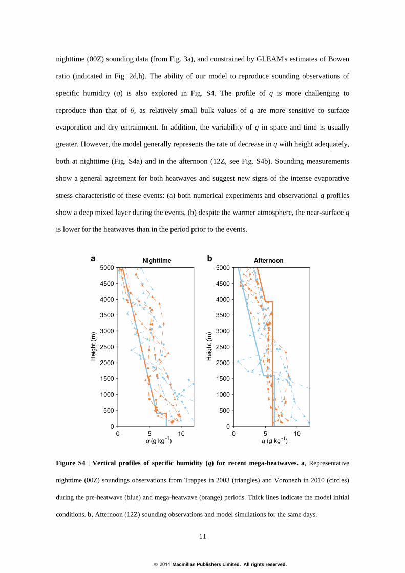
nighttime (00Z) sounding data (from Fig. 3a), and constrained by GLEAM's estimates of Bowen

ratio (indicated in Fig. 2d,h). The ability of our model to reproduce sounding observations of

specific humidity (q) is also explored in Fig. S4. The profile of q is more challenging to

reproduce than that of θ, as relatively small bulk values of q are more sensitive to surface

evaporation and dry entrainment. In addition, the variability of q in space and time is usually

greater. However, the model generally represents the rate of decrease in q with height adequately,

both at nighttime (Fig. S4a) and in the afternoon (12Z, see Fig. S4b). Sounding measurements

show a general agreement for both heatwaves and suggest new signs of the intense evaporative

stress characteristic of these events: (a) both numerical experiments and observational q profiles

show a deep mixed layer during the events, (b) despite the warmer atmosphere, the near-surface q

is lower for the heatwaves than in the period prior to the events.

Figure S4 | Vertical profiles of specific humidity (q) for recent mega-heatwaves. a, Representative

nighttime (00Z) soundings observations from Trappes in 2003 (triangles) and Voronezh in 2010 (circles)

during the pre-heatwave (blue) and mega-heatwave (orange) periods. Thick lines indicate the model initial

conditions. b, Afternoon (12Z) sounding observations and model simulations for the same days.


12

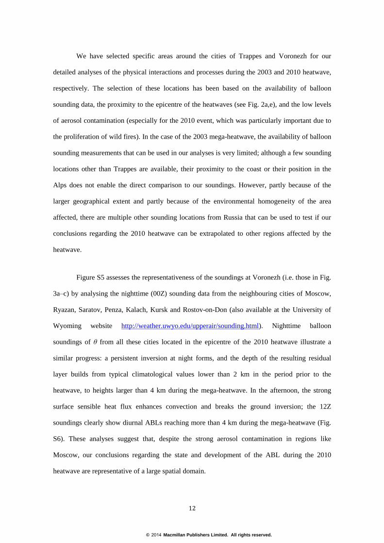
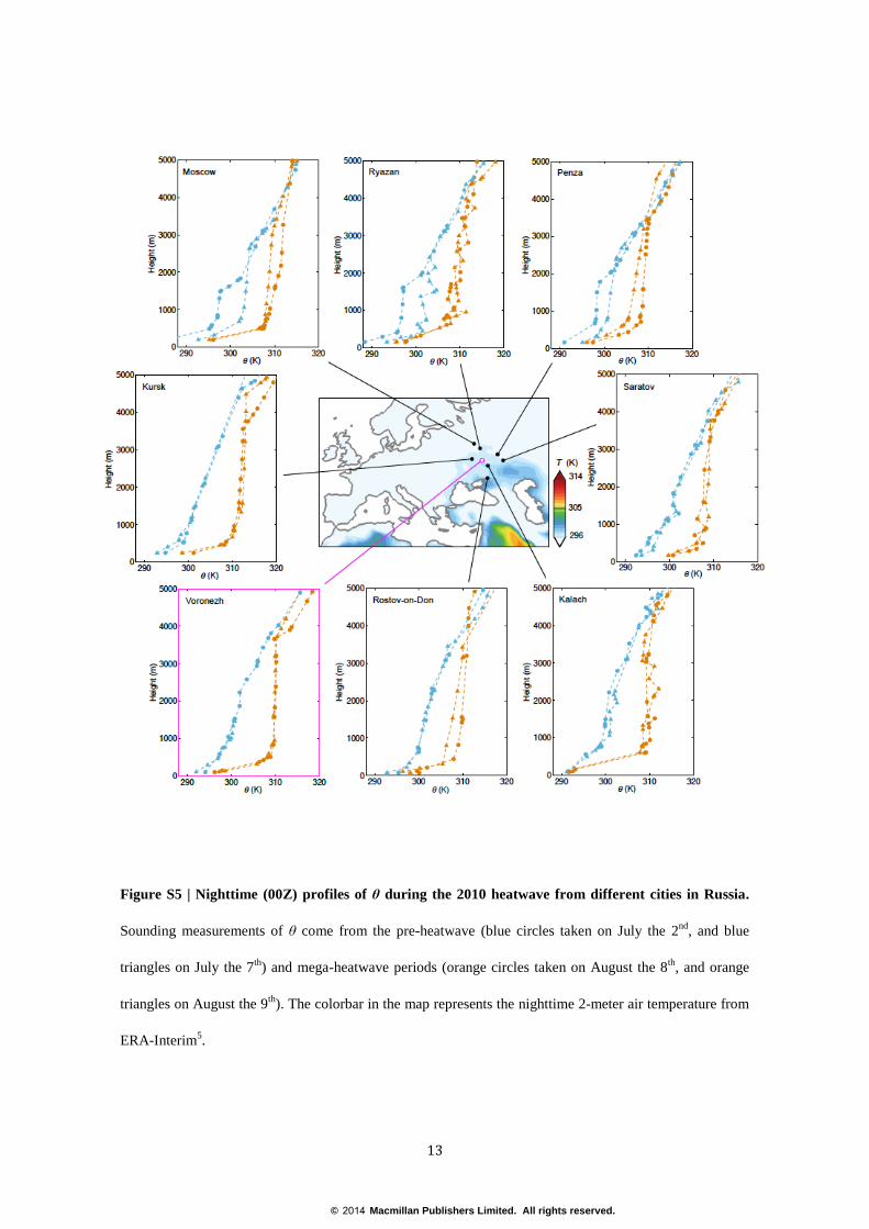
We have selected specific areas around the cities of Trappes and Voronezh for our

detailed analyses of the physical interactions and processes during the 2003 and 2010 heatwave,

respectively. The selection of these locations has been based on the availability of balloon

sounding data, the proximity to the epicentre of the heatwaves (see Fig. 2a,e), and the low levels

of aerosol contamination (especially for the 2010 event, which was particularly important due to

the proliferation of wild fires). In the case of the 2003 mega-heatwave, the availability of balloon

sounding measurements that can be used in our analyses is very limited; although a few sounding

locations other than Trappes are available, their proximity to the coast or their position in the

Alps does not enable the direct comparison to our soundings. However, partly because of the

larger geographical extent and partly because of the environmental homogeneity of the area

affected, there are multiple other sounding locations from Russia that can be used to test if our

conclusions regarding the 2010 heatwave can be extrapolated to other regions affected by the

heatwave.

Figure S5 assesses the representativeness of the soundings at Voronezh (i.e. those in Fig.

3a–c) by analysing the nighttime (00Z) sounding data from the neighbouring cities of Moscow,

Ryazan, Saratov, Penza, Kalach, Kursk and Rostov-on-Don (also available at the University of

Wyoming website http://weather.uwyo.edu/upperair/sounding.html). Nighttime balloon

soundings of θ from all these cities located in the epicentre of the 2010 heatwave illustrate a

similar progress: a persistent inversion at night forms, and the depth of the resulting residual

layer builds from typical climatological values lower than 2 km in the period prior to the

heatwave, to heights larger than 4 km during the mega-heatwave. In the afternoon, the strong

surface sensible heat flux enhances convection and breaks the ground inversion; the 12Z

soundings clearly show diurnal ABLs reaching more than 4 km during the mega-heatwave (Fig.

S6). These analyses suggest that, despite the strong aerosol contamination in regions like

Moscow, our conclusions regarding the state and development of the ABL during the 2010

heatwave are representative of a large spatial domain.


http://weather.uwyo.edu/upperair/sounding.html

13

Figure S5 | Nighttime (00Z) profiles of θ during the 2010 heatwave from different cities in Russia.

Sounding measurements of θ come from the pre-heatwave (blue circles taken on July the 2nd

, and blue

triangles on July the 7th

) and mega-heatwave periods (orange circles taken on August the 8th

, and orange

triangles on August the 9th

). The colorbar in the map represents the nighttime 2-meter air temperature from

ERA-Interim5.


14

Figure S6 | Afternoon (12Z) profiles of θ during the 2010 heatwave from different cities in Russia.

Sounding measurements of θ come from the pre-heatwave (blue circles taken on July the 2nd

, and blue

triangles on July the 7th

) and mega-heatwave periods (orange circles taken on August the 8th

, and orange

triangles on August the 9th

). The colorbar in the map represents the afternoon 2-meter air temperature from

ERA-Interim5.


15

References

1 Miralles, D. G., van den Berg, M., Teuling, R. & De Jeu, R. A. M. Soil moisture-

temperature coupling: A multiscale observational analysis. Geophys. Res. Lett. 39,

L21707 (2012).

2 Crow, W., Miralles, D. & Cosh, M. A quasi-global evaluation system for satellite-based

surface soil moisture retrievals. IEEE Trans. Geosci. Remote Sens. 48, 2516-2527

(2010).

3 Miralles, D. G., Crow, W. T. & Cosh, M. H. Estimating spatial sampling errors in coarse-

scale soil moisture estimates derived from point-scale observations. J. Hydrometeorol.

11, 1423-1429 (2010).

4 Miralles, D. G. et al. El Niño–La Niña cycle and recent trends in continental evaporation.

Nat. Clim. Change 4, 122-126 (2014).

5 Dee, D. P. et al. The ERA-Interim reanalysis: configuration and performance of the data

assimilation system. Quart. J. Roy. Meteorol. Soc. 137, 553-597 (2011).

6 Miralles, D. G., De Jeu, R. A. M., Gash, J. H., Holmes, T. R. H. & Dolman, A. J.

Magnitude and variability of land evaporation and its components at the global scale.

Hydrol. Earth Syst. Sci. 15, 967-981 (2011).

7 Miralles, D. G. et al. Global land-surface evaporation estimated from satellite-based

observations. Hydrol. Earth Syst. Sci. 15, 453-469 (2011).

8 Priestley, C. & Taylor, R. On the assessment of surface heat flux and evaporation using

large-scale parameters. Mon. Weather Rev. 100, 81-92 (1972).

9 Liu, Y. Y., van Dijk, A. I. J. M., McCabe, M. F., Evans, J. P. & de Jeu, R. A. M. Global

vegetation biomass change (1988 - 2008) and attribution to environmental and human

drivers. Global Ecol. Biogeogr. 22, 692-705 (2013).

10 Gash, J. H. An analytical model of rainfall interception by forests. Quart. J. Roy.

Meteorol. Soc. 105, 43-45 (1979).


16

11 Valente, F., David, J. & Gash, J. Modelling interception loss for two sparse eucalypt and

pine forests in central Portugal using reformulated Rutter and Gash analytical models. J.

Hydrol. 190, 141-162 (1997).

12 Miralles, D. G., Gash, J. H., Holmes, T. R. H., de Jeu, R. A. M. & Dolman, A. Global

canopy interception from satellite observations. J. Geophys. Res. 115, D16122 (2010).

13 Chen, M. et al. Assessing objective techniques for gauge-based analyses of global daily

precipitation. J. Geophys. Res. 113 (2008).

14 Rossow, W. B. & Dueñas, E. N. The International Satellite Cloud Climatology Project

(ISCCP) web site: an online resource for research. Bull. Am. Meteorol. Soc. 85, 167-172

(2004).

15 Braverman, A. J., Fetzer, E. J., Kahn, B. H., Manning, E. M., Oliphant, R. B. & Teixeira,

J. P. Massive Dataset Analysis for NASA's Atmospheric Infrared Sounder,

Technometrics 54, 1-15 (2012).

16 Luojus, K. & Pulliainen, J. Global snow monitoring for climate research: Snow Water

Equivalent (SWE) product guide. Helsinki, Finland (2010).

17 Hansen, M. C., Townshend, J. R. G., DeFries, R. S. & Carroll, M. Estimation of tree

cover using MODIS data at global, continental and regional/local scales. Int. J. Remote

Sens. 26, 4359-4380 (2005).

18 Global Soil Data Task Group. Global gridded surfaces of selected soil characteristics,

International Geosphere-Biosphere Programme – Data and Information System. Oak

Ridge National Laboratory Distributed Active Archive Center, Oak Ridge, TE (2010).

19 Tennekes, H. A Model for the Dynamics of the Inversion Above a Convective Boundary

Layer. J. Atmos. Sci. 30, 558-567 (1973).

20 de Arellano, J. V.-G., van Heerwaarden, C. C. & Lelieveld, J. Modelled suppression of

boundary-layer clouds by plants in a CO2-rich atmosphere. Nat. Geosci. 5, 701-704

(2012).


17

21 van Heerwaarden, C. C., de Arellano, J. V.-G., Gounou, A., Guichard, F. & Couvreux, F.

Understanding the daily cycle of evapotranspiration: A method to quantify the influence

of forcings and feedbacks. J. Hydrometeorol. 11, 1405-1422 (2010).

22 Owe, M., de Jeu, R. & Holmes, T. Multisensor historical climatology of satellite-derived

global land surface moisture. J. Geophys. Res. 113, F01002 (2008).

23 Wielicki, B. A. et al. Clouds and the Earth's Radiant Energy System (CERES): An earth

observing system experiment. Bull. Am. Meteorol. Soc. 77, 853-868 (1996).

24 Joyce, R., Janowiak, J., Arkin, P. & Xie, P. CMORPH: A method that produces global

precipitation estimates from passive microwave and infrared data at high spatial and

temporal resolution. J. Hydrometeorol. 5, 487-503 (2004).

25 Liu, Y. Y. et al. Trend-preserving blending of passive and active microwave soil

moisture retrievals. Remote Sens. Environ. 123, 1-18 (2012).


Documents

Mega-heatwave temperatures due to combined soil ... · 1 Supplementary Information Mega-heatwave temperatures due to combined soil desiccation and atmospheric heat buildup Diego G