1/13

Medical diagnostic ultrasound

By Jens E. Wilhjelm and Ole Trier Andersen

Ørsted•DTU, Ørsteds plads, building 348

Technical University of Denmark

2800 Kgs. Lyngby(Ver. 2. 3/3/04) © 2001-2004 by J. E. Wilhjelm & O.T. Andersen

1 IntroductionMedical diagnostic ultrasound is an imaging modality that makes so-called tomographic images (to-

mo = Gr. tome, to cut and graphic = Gr. graphein, to write). It is a diagnostic modality, i.e. it concernsgathering of information without modifying, in any way1, the biological medium from which it gath-ers information. Ultrasound is sound with a frequency over the audible range (20 Hz - 20 kHz), andthe frequencies normally applied in clinical imaging are between 1 MHz and 20 MHz. The sound isgenerated by a transducer that first acts as a loudspeaker sending out an acoustic pulse in a given di-rection and subsequently acts as a microphone in order to record the acoustic echoes generated alongthe path of the emitted pulse. These echoes carry information about the acoustic properties of the tis-sue along the path. The emission of acoustic energy and the recording of the echoes normally takeplace at one and the same transducer, in contrast to CT imaging, where the emitter and recorder arelocated on each side of the patient.

This chapter will explain the generation and reception of ultrasound and the different types of waves.This is followed by a description of ultrasound’s interaction with the medium, which gives rise to theecho information that is used to make images. The different kinds of imaging modalities is next de-scribed, finalized with a description of spatial compounding. The chapter is concluded with a list ofsymbols, terms and references.

2 Generation of ultrasoundUltrasound (as well as sound) needs a medium, in which it can propagate by means of local defor-

mation of the medium. One can think of the medium as being made of small spheres (e.g. the mole-cules in some cases), that are connected with springs. When mechanical energy is transmitted throughsuch a medium, the spheres will oscillate around their resting position. Thus, the propagation of soundis due to a continuous interchange between kinetic energy and potential energy, related to the densityand the elastic properties of the medium, respectively.

The two most simple waves that can exist in solids are longitudinal waves in which the particlemovements occur in the same direction as the propagation (or energy flow), and transversal (or shearwaves) in which the movements occur in a plane perpendicular to the propagation direction. In water

1. To obtain acoustical contact between the transducer and the skin, a small pressure must be applied from the transducer to the skin. In addition to that, ultrasound scanning causes a very small heating of tissue (less than 1°C)

2/13

and soft tissue the waves are mainly longitudinal. The frequency, f, of the particle oscillation is relatedto the wavelength, λ, and the propagation velocity c:

(1)

The sound speed in soft tissue at 37°C is around 1540 m/s, thus at a frequency of 7.5 MHz, the wave-length is 0.2 mm.

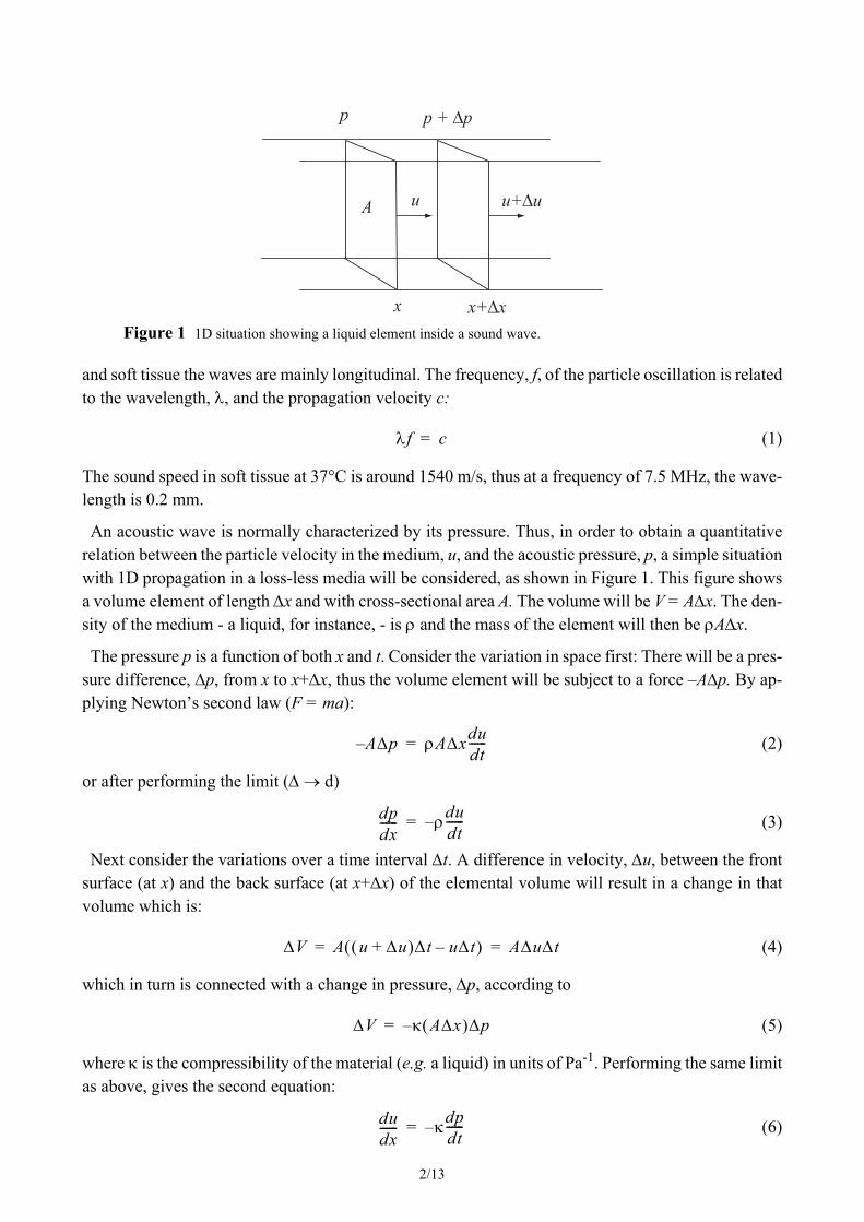
An acoustic wave is normally characterized by its pressure. Thus, in order to obtain a quantitativerelation between the particle velocity in the medium, u, and the acoustic pressure, p, a simple situationwith 1D propagation in a loss-less media will be considered, as shown in Figure 1. This figure showsa volume element of length ∆x and with cross-sectional area A. The volume will be V = A∆x. The den-sity of the medium - a liquid, for instance, - is ρ and the mass of the element will then be ρA∆x.

The pressure p is a function of both x and t. Consider the variation in space first: There will be a pres-sure difference, ∆p, from x to x+∆x, thus the volume element will be subject to a force –A∆p. By ap-plying Newton’s second law (F = ma):

(2)

or after performing the limit (∆ → d)

(3)

Next consider the variations over a time interval ∆t. A difference in velocity, ∆u, between the frontsurface (at x) and the back surface (at x+∆x) of the elemental volume will result in a change in thatvolume which is:

(4)

which in turn is connected with a change in pressure, ∆p, according to

(5)

where κ is the compressibility of the material (e.g. a liquid) in units of Pa-1. Performing the same limitas above, gives the second equation:

(6)

λf c=

u+∆uuA

x x+∆x

p + ∆p p

Figure 1 1D situation showing a liquid element inside a sound wave.

A∆p– ρA∆xdudt------=

dpdx------ ρ– du

dt------=

∆V A u ∆u+( )∆t u∆t–( ) A∆u∆t= =

∆V κ A∆x( )– ∆p=

dudx------ κ– dp

dt------=

3/13

Equations (3) and (6) are the simplest form of the wave equations describing the relation betweenpressure and particle velocity in a loss-less isotropic medium.

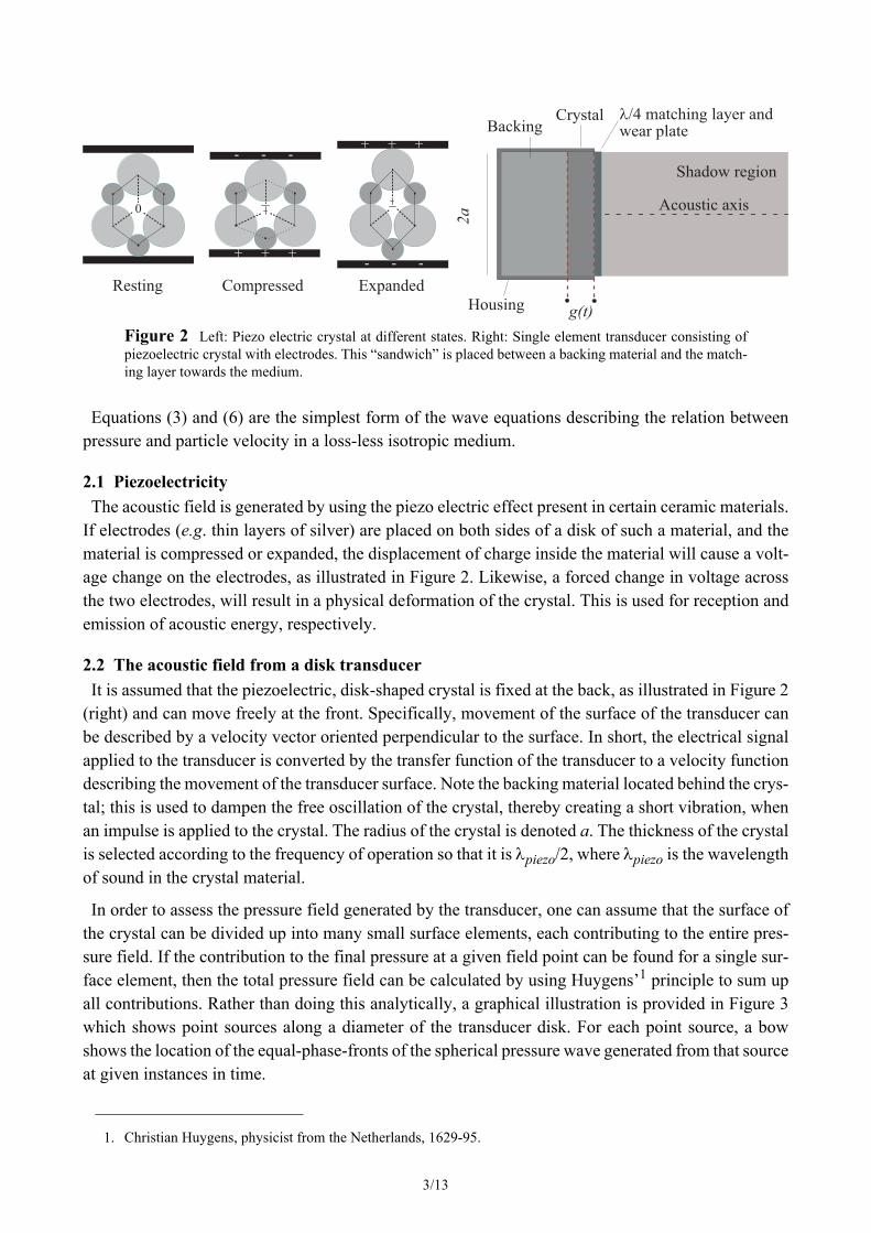
2.1 PiezoelectricityThe acoustic field is generated by using the piezo electric effect present in certain ceramic materials.

If electrodes (e.g. thin layers of silver) are placed on both sides of a disk of such a material, and thematerial is compressed or expanded, the displacement of charge inside the material will cause a volt-age change on the electrodes, as illustrated in Figure 2. Likewise, a forced change in voltage acrossthe two electrodes, will result in a physical deformation of the crystal. This is used for reception andemission of acoustic energy, respectively.

2.2 The acoustic field from a disk transducerIt is assumed that the piezoelectric, disk-shaped crystal is fixed at the back, as illustrated in Figure 2

(right) and can move freely at the front. Specifically, movement of the surface of the transducer canbe described by a velocity vector oriented perpendicular to the surface. In short, the electrical signalapplied to the transducer is converted by the transfer function of the transducer to a velocity functiondescribing the movement of the transducer surface. Note the backing material located behind the crys-tal; this is used to dampen the free oscillation of the crystal, thereby creating a short vibration, whenan impulse is applied to the crystal. The radius of the crystal is denoted a. The thickness of the crystalis selected according to the frequency of operation so that it is λpiezo/2, where λpiezo is the wavelengthof sound in the crystal material.

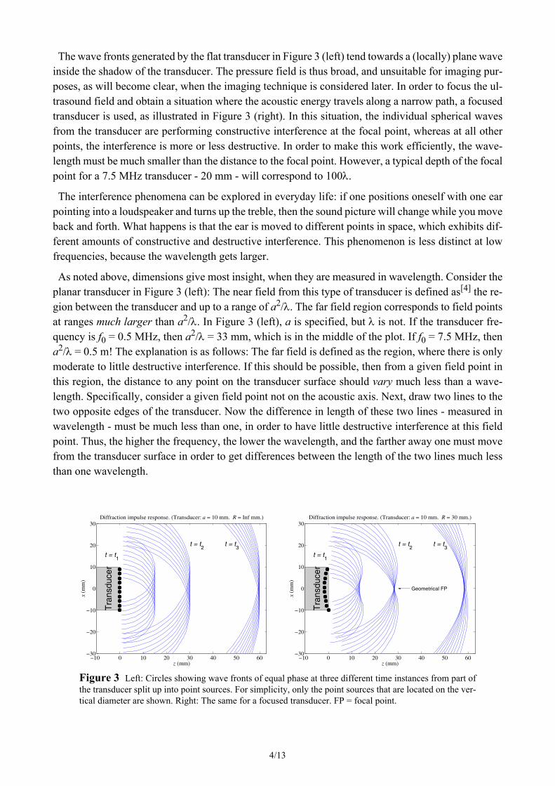
In order to assess the pressure field generated by the transducer, one can assume that the surface ofthe crystal can be divided up into many small surface elements, each contributing to the entire pres-sure field. If the contribution to the final pressure at a given field point can be found for a single sur-face element, then the total pressure field can be calculated by using Huygens’1 principle to sum upall contributions. Rather than doing this analytically, a graphical illustration is provided in Figure 3which shows point sources along a diameter of the transducer disk. For each point source, a bowshows the location of the equal-phase-fronts of the spherical pressure wave generated from that sourceat given instances in time.

1. Christian Huygens, physicist from the Netherlands, 1629-95.

Figure 2 Left: Piezo electric crystal at different states. Right: Single element transducer consisting ofpiezoelectric crystal with electrodes. This “sandwich” is placed between a backing material and the match-ing layer towards the medium.

CrystalBacking

g(t)

Acoustic axis

2a

Housing

λ/4 matching layer and wear plate

Shadow region

Resting Compressed Expanded

++ +

-- -

-- -

++ +

0

4/13

The wave fronts generated by the flat transducer in Figure 3 (left) tend towards a (locally) plane waveinside the shadow of the transducer. The pressure field is thus broad, and unsuitable for imaging pur-poses, as will become clear, when the imaging technique is considered later. In order to focus the ul-trasound field and obtain a situation where the acoustic energy travels along a narrow path, a focusedtransducer is used, as illustrated in Figure 3 (right). In this situation, the individual spherical wavesfrom the transducer are performing constructive interference at the focal point, whereas at all otherpoints, the interference is more or less destructive. In order to make this work efficiently, the wave-length must be much smaller than the distance to the focal point. However, a typical depth of the focalpoint for a 7.5 MHz transducer - 20 mm - will correspond to 100λ.

The interference phenomena can be explored in everyday life: if one positions oneself with one earpointing into a loudspeaker and turns up the treble, then the sound picture will change while you moveback and forth. What happens is that the ear is moved to different points in space, which exhibits dif-ferent amounts of constructive and destructive interference. This phenomenon is less distinct at lowfrequencies, because the wavelength gets larger.

As noted above, dimensions give most insight, when they are measured in wavelength. Consider theplanar transducer in Figure 3 (left): The near field from this type of transducer is defined as[4] the re-gion between the transducer and up to a range of a2/λ. The far field region corresponds to field pointsat ranges much larger than a2/λ. In Figure 3 (left), a is specified, but λ is not. If the transducer fre-quency is f0 = 0.5 MHz, then a2/λ = 33 mm, which is in the middle of the plot. If f0 = 7.5 MHz, thena2/λ = 0.5 m! The explanation is as follows: The far field is defined as the region, where there is onlymoderate to little destructive interference. If this should be possible, then from a given field point inthis region, the distance to any point on the transducer surface should vary much less than a wave-length. Specifically, consider a given field point not on the acoustic axis. Next, draw two lines to thetwo opposite edges of the transducer. Now the difference in length of these two lines - measured inwavelength - must be much less than one, in order to have little destructive interference at this fieldpoint. Thus, the higher the frequency, the lower the wavelength, and the farther away one must movefrom the transducer surface in order to get differences between the length of the two lines much lessthan one wavelength.

Figure 3 Left: Circles showing wave fronts of equal phase at three different time instances from part ofthe transducer split up into point sources. For simplicity, only the point sources that are located on the ver-tical diameter are shown. Right: The same for a focused transducer. FP = focal point.

−10 0 10 20 30 40 50 60−30

−20

−10

0

10

20

30

Tra

nsdu

cer

z (mm)

x (m

m)

Diffraction impulse response. (Transducer: a = 10 mm. R = Inf mm.)

t = t1

t = t2

t = t3

−10 0 10 20 30 40 50 60−30

−20

−10

0

10

20

30

Tra

nsdu

cer

z (mm)

x (m

m)

Diffraction impulse response. (Transducer: a = 10 mm. R = 30 mm.)

Geometrical FP

t = t1

t = t2

t = t3

5/13

3 Types of ultrasound wavesAn ultrasound field from a physical transducer will always show a complicated behaviour as can be

sensed from Figure 3. Each point source emits exactly the same pressure wave. The temporal form ofthis pressure wave could be as exemplified in Figure 6. Thus, the circles in Figure 3 indicate examplesof spatial and temporal locations of each of the individual waveforms that have to be added in orderto construct the total pressure field in front of the transducer (however, the circles in Figure 3 onlyrepresent point sources on a single diameter across the transducer; many more point sources would beneeded to represent the total field from a disk transducer).

In order to obtain some tools to better describe and understand these fields, wave theory makes useof two types of simple, yet theoretical, waves which are introduced here:

The plane wave, where any field parameter is constant in a plane perpendicular to the propagationdirection. As a plane extent over the entire space, it is not physically realizable (but within a givenspace, an approximation to a plane wave can be obtained locally, such as in the shadow of a planartransducer). The other type is a spherical wave. It originates from a point (source) and all acousticparameters are constant at spheres centered around this point.

As a further restriction of the plane wave field, it could be considered monochromatic, that is, it os-cillate at a single frequency, f0. The equation for such a wave in 1D is:

p(x,t) = P0 exp(–j (2πf0t – 2πx/λ)) (7)

where P0 is the pressure magnitude (units in pascal, Pa) x is the distance along the propagation direc-tion and λ = c/f0. (7) is a complex sinusoidal that depends on space and time.

An important concept in wave theory is diffraction. Ironically, the term diffraction can best be de-scribed by what it is not: “Any propagating scalar field which experiences a deviation from a rectilin-ear propagation path, when such deviation is not due to reflection or refraction, is generally said toundergo diffraction effects. This description includes the bending of waves around objects in theirpath. This bending is brought about by the redistribution of energy within the wave front as it passesby an opaque body.”[3] Examples where diffraction effects are significant are: Propagation of wavesthrough an aperture in a baffle (i.e. a hole in a plate) and radiation from sources of finite size.[3] Withthe above definition, the only non-diffracted wave is the plane wave.

4 Ultrasound’s interaction with the medium

4.1 Reflection and transmissionThe plane wave can be used when explaining reflection and transmission from one medium to an-

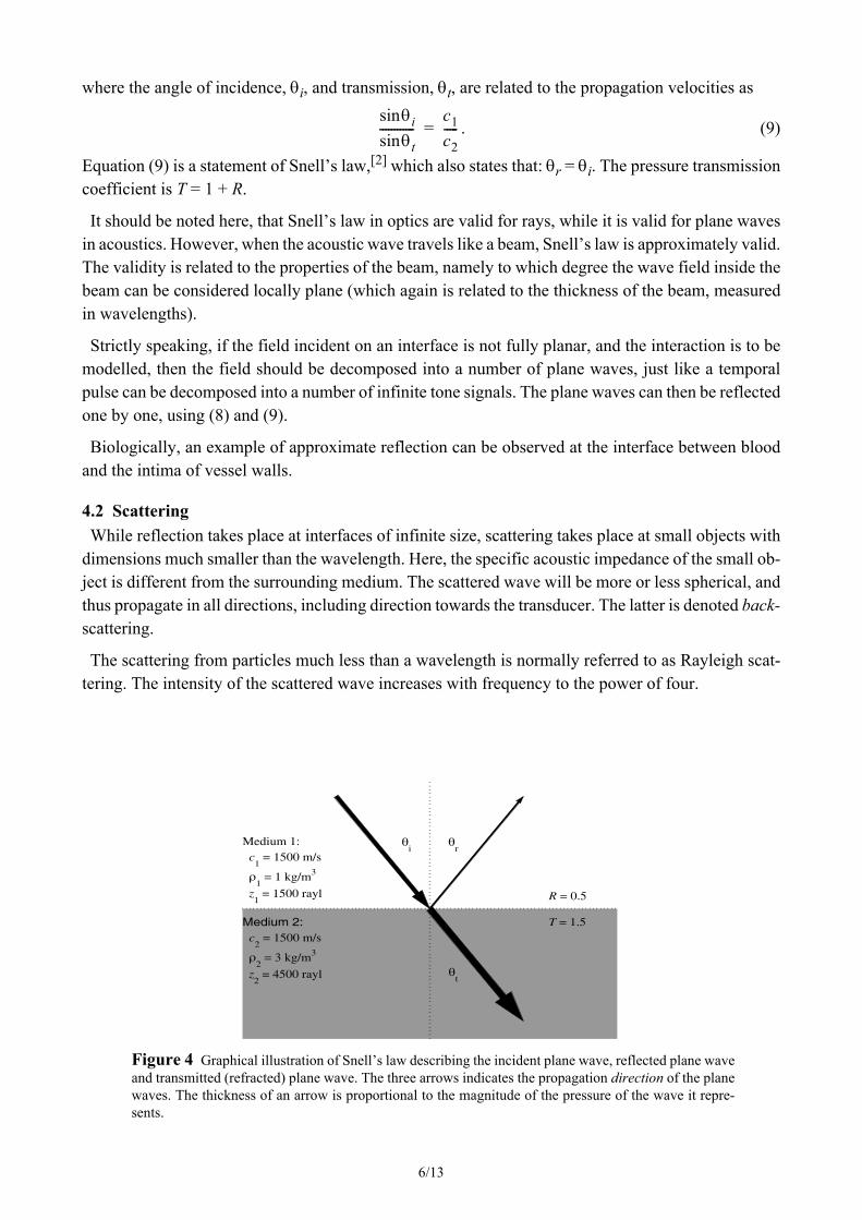
other, when the interface between the media is planar. For this purpose the specific acoustic impe-dance, z, is introduced. In a homogeneous medium it is defined as the ratio of pressure to particlevelocity in a progressing plane wave, and can be shown to be the product of the density, ρ, and acous-tic propagation velocity c of the medium. Thus, medium 1 is specified in terms of its density, ρ1, andacoustic propagation velocity c1. The specific acoustic impedance for this medium is z1 = ρ1c1, withunits: kg/(m2s). Likewise for medium 2: z2 = ρ2c2. The interaction of ultrasound with this interfaceis illustrated in Figure 4, where an incident plane wave is reflected and transmitted at the interfacebetween medium 1 and medium 2. The (pressure) reflection coefficient between the two media is:

(8)Rz2 θtcos( ) z1 θicos( )⁄–⁄z2 θtcos( )⁄ z1 θicos( )⁄+------------------------------------------------------------=

6/13

where the angle of incidence, θi, and transmission, θt, are related to the propagation velocities as

. (9)

Equation (9) is a statement of Snell’s law,[2] which also states that: θr = θi. The pressure transmissioncoefficient is T = 1 + R.

It should be noted here, that Snell’s law in optics are valid for rays, while it is valid for plane wavesin acoustics. However, when the acoustic wave travels like a beam, Snell’s law is approximately valid.The validity is related to the properties of the beam, namely to which degree the wave field inside thebeam can be considered locally plane (which again is related to the thickness of the beam, measuredin wavelengths).

Strictly speaking, if the field incident on an interface is not fully planar, and the interaction is to bemodelled, then the field should be decomposed into a number of plane waves, just like a temporalpulse can be decomposed into a number of infinite tone signals. The plane waves can then be reflectedone by one, using (8) and (9).

Biologically, an example of approximate reflection can be observed at the interface between bloodand the intima of vessel walls.

4.2 ScatteringWhile reflection takes place at interfaces of infinite size, scattering takes place at small objects with

dimensions much smaller than the wavelength. Here, the specific acoustic impedance of the small ob-ject is different from the surrounding medium. The scattered wave will be more or less spherical, andthus propagate in all directions, including direction towards the transducer. The latter is denoted back-scattering.

The scattering from particles much less than a wavelength is normally referred to as Rayleigh scat-tering. The intensity of the scattered wave increases with frequency to the power of four.

θisinθtsin

------------c1c2-----=

θi

θr

θt

Medium 1: c

1 = 1500 m/s

ρ1 = 1 kg/m3

z1 = 1500 rayl

Medium 2: c

2 = 1500 m/s

ρ2 = 3 kg/m3

z2 = 4500 rayl

R = 0.5

T = 1.5

Figure 4 Graphical illustration of Snell’s law describing the incident plane wave, reflected plane waveand transmitted (refracted) plane wave. The three arrows indicates the propagation direction of the planewaves. The thickness of an arrow is proportional to the magnitude of the pressure of the wave it repre-sents.

7/13

Biologically, scattering can be observed in most tissue and especially blood, where the red bloodcells are the predominant cells. They have a diameter of about 7 µm much smaller than the wavelengthof clinical ultrasound.

4.3 AbsorptionAbsorption is the conversion of acoustic energy into heat. The mechanisms of absorption are not ful-

ly understood, but relate, among other things, to the friction loss in the springs, mentioned in Subsec-tion 2. More details on this can be found in the literature.[2]

Absorption by itself can be observed by sending ultrasound through a viscous liquid such as oil.

4.4 AttenuationThe loss of intensity (or energy) of the forward propagating wave due to reflection, refraction, scat-

tering and absorption is denoted attenuation. The intensity is a measure of the power through a givencross section; thus the units are W/m2. It can be calculated as the product between particle velocityand pressure: I = pu = p2/z. If I(0) is the intensity of the pressure wave at some reference point in spaceand I(x) is the intensity at a point x further along the propagation direction then the attenuation of theacoustic pressure wave can be written as:

I(x) = I(0)e–αx (10)

where α (in units of m-1) is the attenuation coefficient. α depends on the tissue type (and for sometissue types like muscle, also on the orientation of the tissue fibres) and is approximately proportionalwith frequency.

Scattering

Att

enua

tion

time

Transducer

Reflection, 90°

Refraction

Absorption

Diffuse scattering

Voltage

Z1 =

ρ1 c

1

Reflection, ≠90°

Z2 =

ρ2 c

2

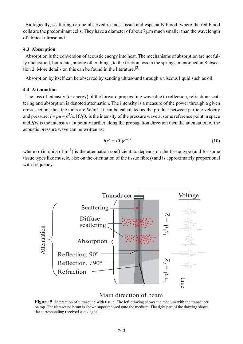
Main direction of beamFigure 5 Interaction of ultrasound with tissue. The left drawing shows the medium with the transduceron top. The ultrasound beam is shown superimposed onto the medium. The right part of the drawing showsthe corresponding received echo signal.

8/13

As a rule of thumb, the attenuation in biological media is 1 dB/cm/MHz. As an example, considerultrasound at 7.5 MHz. When a wave at this frequency has travelled 5 cm in tissue, the attenuationwill (on average) be 1 dB/cm/MHz x 5 cm x 7.5 MHz = 37.5 dB. For bone, the attenuation is about30 dB/MHz/cm. If these two attenuation figures are converted to intensity half-length (the distancecorresponding to a loss of 50 %) at 2 MHz, it would correspond to 15 mm in soft tissue and 0.5 mmin bone.

4.5 An example of ultrasound’s interaction with biological tissueWhen an ultrasound wave travels in a biological medium all the above mechanisms will take place.

Reflection and scattering will not take place as two perfectly distinct phenomena, as they were de-scribed above. The reason is that the body does not contain completely smooth interfaces of infinitesize. Likewise, the scattered wave from infinitesimally small point objects will also be infinitesimallysmall in amplitude and thereby not measurable.

The scattered wave moving towards the transducer as well as the reflected wave moving towards thetransducer will be denoted the echo in this book.

The effects in Subsection 4.1 - 4.4 are illustrated in Figure 5.

The absorption continuously takes place along the acoustic beam, as media 1 and media 2 (indicatedby their specific acoustic impedances) are considered lossy.

Consider the different components of the medium: Scattering from a single inhomogeniety is illus-trated at the top of the medium. Below is a more realistic situation where the echoes from many scat-terers create an interference signal. If a second identical scattering structure is located below the first,then the interference signal will be roughly identical to the interference signal from the first. The over-all amplitude, however, will be a little lower, due to the absorption and the loss due to the first groupof scatterers. Notice that the interference signal varies quite a bit in amplitude.

The emitted signal next encounters a thin planar structure, resulting in a well-defined strong echo.

Next, an angled interface is encountered, giving oblique incidence and thus refraction, according to(8) and Figure 4. The change in specific acoustic impedance is the same as above, but due to the non-perpendicular incidence, less energy is reflected back. The transmitted wave undergoes refraction,and thus scatterers located below this interface will be imaged geometrically incorrectly.

cd2

Time

Rec

eived

sig

nal d Ultrasound beam

Transducer Point reflector

Volt

age

Emitted pulse Echo

signal

gr(t)

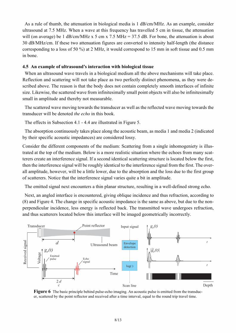
Figure 6 The basic principle behind pulse-echo imaging. An acoustic pulse is emitted from the transduc-er, scattered by the point reflector and received after a time interval, equal to the round trip travel time.

t

t

Envelope

detection

log(·)

Input signal

Scan line Depth

gr(t)

|gr(t)|~

9/13

5 Imaging

5.1 A-modeThe basic concept behind medical diagnostic ultrasound is shown in Figure 6, which also shows the

simplest mode of operation, A-mode. In the situation in Figure 6 (left) a single point scatterer is lo-cated in front of the transducer at depth d. A short pulse is emitted from the transducer, and at time2d/c, the echo from the point target is received by the same transducer. Thus, the deeper the point scat-terer is positioned, the later the echo from this point scatterer arrives. If many point scatterers (andreflectors) are located in front of the transducer, the total echo can be found by simple superposition,as this is a linear system, when the pressure amplitude is sufficiently low.

The received signal, gr(t), is Hilbert transformed to grH(t) in order to create the corresponding ana-lytical signal r(t) = gr(t) + jgrH(t). Twenty time the log of the envelope of this signal, 20log| (t)|, isthen the envelope in dB, which can be displayed as a gray scale line, as shown in Figure 6 (right). Sucha gray scale bar is called a scan line, which is also the word used for the imaginary line in tissue, alongwhich gr(t) is recorded. Note, that because the envelope process is not fully linear, the scanner doesnot constitute a fully linear system.

5.2 M-modeIf the sequence of pulse emission and reception is repeated infinitely, and the scan lines are placed

next to each other (with new ones to the right), motion mode, or M-mode, is obtained. The verticalaxis will be depth in meters downwards, while the horizontal axis will be time in seconds pointing tothe right. This mode can be useful when imaging heart valves, because the movement of the valveswill make distinct patterns in the “image”.

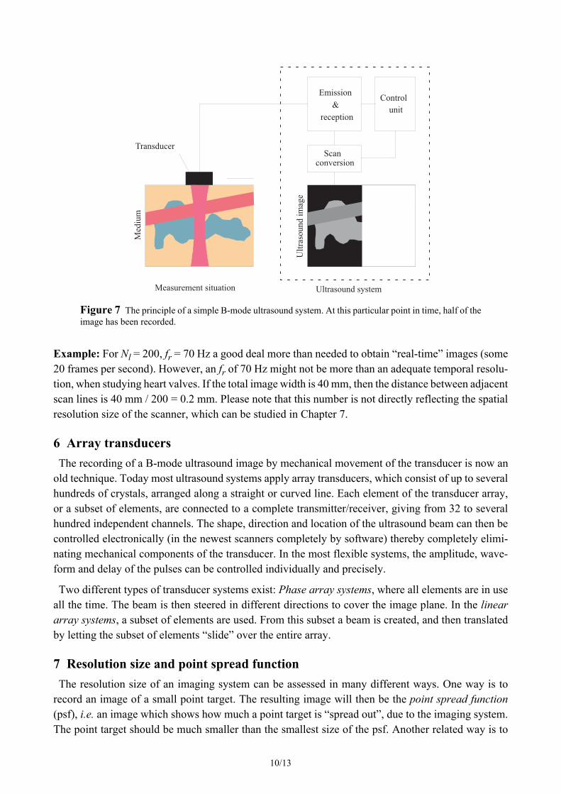
5.3 B-modeBrightness or B-mode is obtained by physically moving the scan line to a number of adjacent loca-

tions. The principle is shown in Figure 7. In this figure, the transducer is moved in steps mechanicallyacross the medium to be imaged. Typically 100 to 300 steps are used, with a spacing between 0.25λand 5λ. At each step, a short pulse is emitted followed by a period of passive registration of the echo.In order to prevent mixing the echoes from different scan lines, the registration period has to be longenough to allow all echoes from a given emitted pulse to be received. This will now be considered indetail.

Assume that the average attenuation of ultrasound in human soft tissue is a in units dB/MHz/cm. Ifthe smallest echo that can be detected - on average - has a level of γ in dB, relative to the echo fromtissue directly under the transducer, then the maximal depth from where an echo can be expected is γ= a f0 2Dmax or

(11)

Example: According to a rule of thumb, the average attenuation of ultrasound in human soft tissue is1 dB/MHz/cm. Assume that γ = 80 dB. At f0 = 7.5 MHz (11) gives Dmax = 5.3 cm.

The time between two emissions will then be Tr = 2Dmax/c, which is the time it take the emitted pulseto travel to Dmax and back again. If there are Nl scan lines per image, then the frame-rate (number ofimages per second produced by the scanner) will be

fr = (Tr Nl)–1. (12)

g̃ g̃

Dmaxϒ

2af0----------=

10/13

Example: For Nl = 200, fr = 70 Hz a good deal more than needed to obtain “real-time” images (some20 frames per second). However, an fr of 70 Hz might not be more than an adequate temporal resolu-tion, when studying heart valves. If the total image width is 40 mm, then the distance between adjacentscan lines is 40 mm / 200 = 0.2 mm. Please note that this number is not directly reflecting the spatialresolution size of the scanner, which can be studied in Chapter 7.

6 Array transducersThe recording of a B-mode ultrasound image by mechanical movement of the transducer is now an

old technique. Today most ultrasound systems apply array transducers, which consist of up to severalhundreds of crystals, arranged along a straight or curved line. Each element of the transducer array,or a subset of elements, are connected to a complete transmitter/receiver, giving from 32 to severalhundred independent channels. The shape, direction and location of the ultrasound beam can then becontrolled electronically (in the newest scanners completely by software) thereby completely elimi-nating mechanical components of the transducer. In the most flexible systems, the amplitude, wave-form and delay of the pulses can be controlled individually and precisely.

Two different types of transducer systems exist: Phase array systems, where all elements are in useall the time. The beam is then steered in different directions to cover the image plane. In the lineararray systems, a subset of elements are used. From this subset a beam is created, and then translatedby letting the subset of elements “slide” over the entire array.

7 Resolution size and point spread functionThe resolution size of an imaging system can be assessed in many different ways. One way is to

record an image of a small point target. The resulting image will then be the point spread function(psf), i.e. an image which shows how much a point target is “spread out”, due to the imaging system.The point target should be much smaller than the smallest size of the psf. Another related way is to

Emission

&

reception

Control

unit

Scan conversion

TransducerM

ediu

m

Ult

raso

und i

mag

e

Measurement situation Ultrasound system

Figure 7 The principle of a simple B-mode ultrasound system. At this particular point in time, half of theimage has been recorded.

11/13

image two point targets with different separations, and see how close they can be positioned and stillbe distinguishable.

The –3 dB width of the psf in the vertical and horizontal image direction will then be a quantitativemeasure for the resolution size. The two directions corresponds to the depth and lateral direction inthe recording situation, respectively.

The resolution in the depth direction (axial resolution) can be appreciated from the echo signal inFigure 6. This signal was created by emitting the smallest number of periods. Because axial resolutioncan be improved only by decreasing the length of the echo signal from the point target, the centre fre-quency of the transducer must be increased to improve resolution. But increasing f0 will increase at-tenuation as well, as discussed in Subsection 4.4. The consequence is that centre frequency andresolution size is always traded off.

This topic is treated again in the chapter on image quality in this web book.

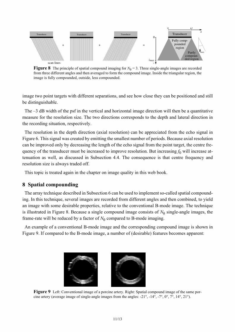
8 Spatial compoundingThe array technique described in Subsection 6 can be used to implement so-called spatial compound-

ing. In this technique, several images are recorded from different angles and then combined, to yieldan image with some desirable properties, relative to the conventional B-mode image. The techniqueis illustrated in Figure 8. Because a single compound image consists of Nθ single-angle images, theframe-rate will be reduced by a factor of Nθ compared to B-mode imaging.

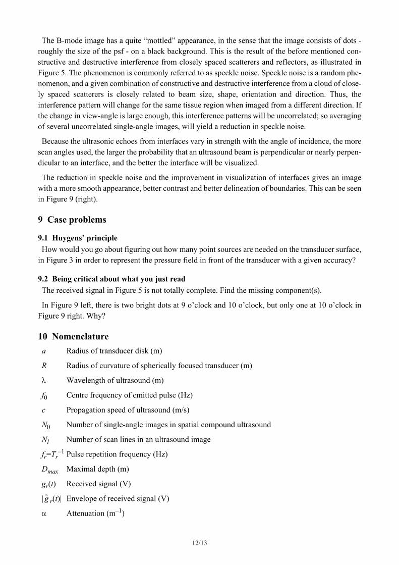
An example of a conventional B-mode image and the corresponding compound image is shown inFigure 9. If compared to the B-mode image, a number of (desirable) features becomes apparent:

Figure 8 The principle of spatial compound imaging for Nθ = 3. Three single-angle images are recordedfrom three different angles and then averaged to form the compound image. Inside the triangular region, theimage is fully compounded, outside, less compounded.

Transducer Transducer

z

Transducer0

Transducer

+ + =

compoun-ded region

Partly

zmax

max

scan lines

xD0

Fully comp-

regionpounded

Figure 9 Left: Conventional image of a porcine artery. Right: Spatial compound image of the same por-cine artery (average image of single-angle images from the angles: -21°, -14°, -7°, 0°, 7°, 14°, 21°).

12/13

The B-mode image has a quite “mottled” appearance, in the sense that the image consists of dots -roughly the size of the psf - on a black background. This is the result of the before mentioned con-structive and destructive interference from closely spaced scatterers and reflectors, as illustrated inFigure 5. The phenomenon is commonly referred to as speckle noise. Speckle noise is a random phe-nomenon, and a given combination of constructive and destructive interference from a cloud of close-ly spaced scatterers is closely related to beam size, shape, orientation and direction. Thus, theinterference pattern will change for the same tissue region when imaged from a different direction. Ifthe change in view-angle is large enough, this interference patterns will be uncorrelated; so averagingof several uncorrelated single-angle images, will yield a reduction in speckle noise.

Because the ultrasonic echoes from interfaces vary in strength with the angle of incidence, the morescan angles used, the larger the probability that an ultrasound beam is perpendicular or nearly perpen-dicular to an interface, and the better the interface will be visualized.

The reduction in speckle noise and the improvement in visualization of interfaces gives an imagewith a more smooth appearance, better contrast and better delineation of boundaries. This can be seenin Figure 9 (right).

9 Case problems

9.1 Huygens’ principleHow would you go about figuring out how many point sources are needed on the transducer surface,

in Figure 3 in order to represent the pressure field in front of the transducer with a given accuracy?

9.2 Being critical about what you just readThe received signal in Figure 5 is not totally complete. Find the missing component(s).

In Figure 9 left, there is two bright dots at 9 o’clock and 10 o’clock, but only one at 10 o’clock inFigure 9 right. Why?

10 Nomenclaturea Radius of transducer disk (m)

R Radius of curvature of spherically focused transducer (m)

λ Wavelength of ultrasound (m)

f0 Centre frequency of emitted pulse (Hz)

c Propagation speed of ultrasound (m/s)

Nθ Number of single-angle images in spatial compound ultrasound

Nl Number of scan lines in an ultrasound image

fr=Tr–1 Pulse repetition frequency (Hz)

Dmax Maximal depth (m)

gr(t) Received signal (V)

| r(t)| Envelope of received signal (V)

α Attenuation (m–1)

g̃

13/13

p Pressure (Pa)

z Specific acoustic impedance (rayl = kg/(m2s))

ρ Physical density of medium (kg/m3)

κ Compressibility of a medium (Pa–1)

11 GlossaryRefraction “The deviation of light in passing obliquely from one medium to another of different

density. The deviation occurs at the surface of junction of the two media, which is known as the re-fracting surface. The ray before refraction is called incident ray; after refraction it is the refracted ray.The point of junction of the incident and the refracted ray is known as the point of incidence. [...]”.[1]

Isotropic “Similar in all directions with respect to a property, as in a cubic crystal or a piece ofglass.”[1]

dB A magnitude variable, such as pressure, p, in Pa, can be written in as 20log10(p/pref) dB, wherepref is some given reference pressure, needed to render the argument to the logarithm dimension less.Likewise intensities, I, can be written as: 10log10(I/Iref) dB.

12 References[1] Dorland’s Illustrated Medical Dictionary. 27th edition. W. B. Saunders Co., Philadelphia, PA,

USA. 1988.

[2] Kinsler LE, Frey AR, Coppens AB & Sanders JV: Fundamentals of acoustics. 3rd ed. John Wiley & sons, Inc. New York, NY, USA, 1982.

[3] Orofino, DP: Analysis of angle dependent spectral distortion in pulse-echo ultrasound. PhD dis-sertation, Department of Electrical Engineering, Worcester Polytechnic Institute, August 1992, USA.

[4] Kino, GS: Acoustic waves. Prentice-Hall, Inc. Englewood Cliffs, New Jersey, USA. 1987.