Embed Size (px)
Citation preview

Example of non-linear filtering: Median filtering
Median filtering is a non-linear operation:
Odd window sizes are commonly used in median filtering:3 × 3 ; 5 × 5 ; 7 × 7
Generally: median { xm + ym } ≠
median { xm } + median { ym }example with signal sequences (length = 3):
example: 5-pixel cross-shaped window
For even-sized windows ( 2 K values ): the filter sorts the values then takes the average of the two middle values :
Output value ( Kth classified value + (K+1)th classified value )2=
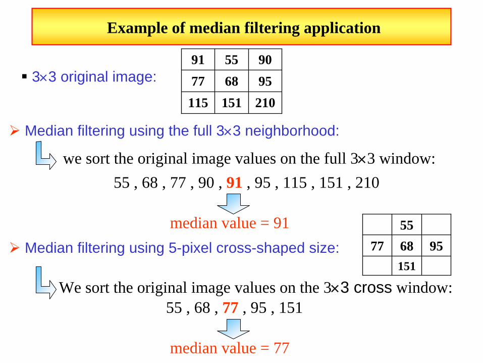
Example of median filtering application
Median filtering using the full 3×3 neighborhood:
91 55 9077 68 95115 151 210
5577 68 95
151
3×3 original image:
we sort the original image values on the full 3×3 window:55 , 68 , 77 , 90 , 91 , 95 , 115 , 151 , 210
median value = 91Median filtering using 5-pixel cross-shaped size:
We sort the original image values on the 3×3 cross window:55 , 68 , 77 , 95 , 151
median value = 77

Comparison: median filter and averaging filter
Original image “Eight.tif” with added ‘salt-and-pepper’ noise then filtered with a (3-by-3) averaging filter and a (3-by-3) median filter.
Original Image After Adding Noise
Noise Average
Median
The median filter does a better job of removing ‘salt-and-pepper’ noise, with less blurring of edges.
Observation:

Exercise Chapter 4 – Comparison: non-linear filtering vs. linear filtering
Unlike filtering by convolution (linear filtering), non-linear filtering uses neighboring pixels
according to a non-linear law. The median filter (specific case of rank filtering), which is used
in this exercise, is a classical example of these filters. Just like the linear filters, a non-linear
filter is performed by using a neighborhood.
1. To create a noisy image
Load the image BOATS_LUMI.BMP. Update the path browser.
The aim is to compare the effects of a linear and a non-linear filtering used to reduce the noise
in an original image.
The Matlab function imnoise allows you to add different classical noises to an image. Use this
function for computing the noisy image of BOATS_LUMI (use a “salt-and-pepper” noise).
Display the noisy image and explain how this kind of noise is added?
2. Application of a linear filtering
We want to reduce the noise in the image. Let us consider a (3 × 3) averaging filter for
reducing the noise. Its convolution kernel is:
111
111
111
.91
Perform this filter (by using the Matlab function imfilter), and visualize the noisy image.
Interpret the result.
3. Application of a non-linear filtering
We want now to reduce the noise by using a (3 × 3) median filtering. You can implement this
filtering with the Matlab function medfilt2. Explain how this function works. Process the
noisy image by performing this median filtering and visualize the results. Explain the
differences between these results and the results of the linear filtering.

Exercise solution: Linear filtering vs. non-linear filtering 1 – Here are the commands to visualize the noisy im age BOATS_LUMI: I=imread(‘BOATS_LUMI.BMP’) ; % to read the grayscal e image IB = imnoise(I,'salt & pepper'); % to create the no isy image figure(1) subplot(1,2,1) subimage(I) title(‘Original Image’) subplot(1,2,2) subimage(IB) title(‘Noisy Image’) Here are the images displayed:
The ‘salt-and-pepper’ noise consists of random pixe ls being set to black or white (the extremes of the gray level range). This kind of impulse noise can be generated by imag e digitalization or during image transmission.

2 – Here are the commands to perform the 3-by-3 ave raging filter: % Averaging filter N = ones(3)/9 ; % convolution kernel If1 = imfilter(IB,N) ; figure(2) image(If1) title('Noisy image filtered by a 3-by-3 averaging f ilter’) v=0:1/255:1; colormap([v' v' v']); % LUT for displa ying in gray levels Here is the image displayed:
The “salt-and-pepper” noise is not significantly re duced. We can still easily distinguish the noisy pixels. Each output pi xel value is the mean value of all the values of its neighboring pixels, therefore when a noisy pixel is included in the neighborhood, its extreme value (0 and 255) is used to compute the mean value:
All the pixels of this image are set to the luminan ce value 8 except one noisy pixel which has the luminance value 255. The output value of the surrounded pixel (and of all pixels whose neighborh ood contains the value 255) is equal to: (8 ×8+255)/9 ≈ 35. The output value of this pixel is thus not representative of its neighborhood, the noise i s not enough reduced. This linear filtering is not appropriate for reduci ng the impulse noise.

3 – Here are the commands to perform the median fil tering: % Median filtering If2 = medfilt2(IB,[3 3]) ; % 3-by-3 median filterin g figure(3) image(If2) title('Noisy Image filtered by a 3-by-3 median filt er’) v=0:1/255:1; colormap([v' v' v']); % LUT for displa ying in gray levels Here is the image visualized:
The “salt-and-pepper” noise is significantly reduce d. This median filtering does a better job of removing noise, with less blur ring of edges. The filter sorts the neighboring values of a pixel, the output value is then the median value of all these sorted values (non-li near operator):
Let us consider the previous example: the pixel val ues are sorted by increasing order: 0, 8, 8, 8, 8, 8, 8, 8, 255. The median value is 8. The extreme luminance values 0 and 255 have no effect on the output value by using this non-linear filtering. The median filtering is efficient for reducing the impulse noise.

Example of a morphological filtering application, Rice Grains (1/2)
♦ Preprocessing:b : Binarization and regularization of the shape
c : Deletion of the boundary objects (grains on the image boundaries)
a : Original Image (rice grains)
a : original image b : segmentation of a c : internal grains

e : Broken grains
f : Grains with connected components
d : Intact grains
♦ Separation and classification of the grains by morphological operations:
Example of a morphological filtering application, Rice Grains (2/2)
Possibility of measuring and counting the rice grains, etc.
d : intact grains e : broken grains f : connected components

Morphological closing to smooth and to regularize the shapes, then binarization of the grayscale image by thresholding
Morphological opening along 2 known diagonal directions for detecting the lines
Detection and localization of intersection points
Motion detection, measurement of sheet deformations, etc.
Example of morphological filtering application, metal sheets

Morphological filtering
♦ Objectives:
Obtaining sets of connected points having simple shape (binary image)
Obtaining principal connected components ( in lower numbers )
Regularization of the shape of the image signal
♦ Applications:
Size filtering
Object counting
Object measurement

Morphological operations
Case of binary images
Chapter 4
NON-LINEAR FILTERING

Recall : classical binary operators
• operator AND : Z = X AND Y ( notation Z = X . Y )X Y Z0 0 01 0 00 1 01 1 1
X Y Z0 0 01 0 10 1 11 1 1
X Z0 11 0
• operator OU : Z = X OU Y ( notation Z = X + Y )
• operator NON : Z = X
X , Y , Z : Boolean variables ⇒ possible states : ‘0’ or ‘1’
A variable which can take only two states (true or false, turned on or turned off, top or
bottom, positive or negative, black or white, etc.) is called a Boolean variable. Typically we
allow the value ‘1’ to one of the two states, and the value ‘0’ to the other state.
Three classical binary operators are defined:
- the operator ‘AND’, the output value is ‘true’ only if both input values are ‘true’;
- the operator ‘OR’, the output value is ‘true’ if at least one of the two input values is
‘true’;
- the operator ‘NOT, the output value is the opposite value of the input value.
“Truth tables” (which define the operators) are displayed on the bottom figure. Commonly
we write “A . B” instead of “A and B”, and “A + B” instead of “A or B”.
Note that several other operators are defined from these classical operators: the operator
‘NOR’ (i.e. ‘not or’), the operator ‘NAND’ (i.e. ‘not and’), the operator ‘XOR’ (i.e.
‘eXclusive or’), …

� Concept :
• set theory description of images.
• take into account the shape of the image structured components.
• basic application: two-level image processing, extension to
multilevel image processing
� Operators :
• 2 basic operators⇒ “EROSION” and “DILATION”
• Combination of these 2 opertors
⇒ 2 complementary operators:
“OPENING” and “CLOSING”
• Operators depending on a structuring element.
Morphological filtering
Morphological filtering is based on mathematical morphology (set theory description of the
images). The morphological operators privilege the shape rather than the signal amplitude.
They can be used to process both binary images (two levels: white or black) and grayscale
images.
We will just present the binary morphological filtering here. This non-linear filtering is based
on two basic operators (erosion and dilation) and two complementary operators which result
from the combination of the two first basic operators (opening and closing).
A structuring element is used to define a neighborhood shape and size for morphological
operations, including dilation and erosion.
We will now define all these concepts.

Binary Image
• L(m,n) ∈∈∈∈ {0, 1} ∀∀∀∀(m,n) ∈∈∈∈ S image support
L = 0 “background” pixel
L = 1 “Object” pixel
� 2 categories : « Background », « Object »
• Object(s) : X
X = { p ∈ S / L(p) = 1 }
A binary image is an image whose pixels (m, n) take their value from among two possible
luminance values. These two possible values are conventionally 0 (background) and 1
(objects).
The objects ‘X’ are defined as the set of pixels ‘P’ with affix ‘p’ that belong to the image
support ‘S’ and such as their luminance value L(p) is equal to 1:
X = { p ∈S / L(p) = 1 }
A binary image can be created by different methods: a digitalization with only two
reconstruction levels, or a binarization of a grayscale image by using its histogram to choose
an appropriate threshold (cf. exercise « Binarization » of chapter 2).

- a - - b - - c –
1-D structuring element 2-D structuring elements
B = {p so that L(p) = 1}
� structuring element
symmetry:
Structuring Elements (binary images)
set of pixels at ‘1’ on a support with the origin located at
(0, 0) coordinates (red pixel)
� 3 typical examples:
“support center”
� Structuring element :
The structuring element B is a set of pixels at luminance value ‘1’. The structural element
includes generally the origin O(0, 0), but not necessarily.
Let B be a structuring element composed by a set of pixels P of affix p. We define then the
symmetrical structuring element B as being the set of pixels of affix ‘-p’.
Example :

Structuring Element
Erosion by (b)Erosion by (a)
(a) “4-connected” structuring element
(b) “8-connected” structuring element
Original ImageExample :
• X � B : set of pixels p in S such for every p, Bp is fully
included in the object X
Morphological Erosion (by B)
Notation X � B
Definition X � B = { p ∈ S so that Bp ⊆ X}
where Bp is the translation of B by p
The erosion of an object X by the structural element B is noted « XӨB ». Let Bp denote
the translation of B so that its origin is at p. The erosion of objects X by the structuring
element B is then the set of all pixels P(p) in the image support S such that Bp is a subset of X:
X B = { p∈S, so that Bp⊆X}
The figure above displays two erosions which are performed on the same original image but
with two different structuring elements:
- case a: 4-connected structuring element (the origin has 4 neighboring). Each pixel of
the image support which has the luminance value 0, or one of whose 4 neighboring
pixels has the value 0, is set to 0 after filtering.
- case b: 8-connected structuring element (the origin has 8 neighboring). Each pixel of
the image support which has the luminance value 0, or one of whose 8 neighboring
pixels has the value 0, is set to 0 after filtering.
We can observe that the two erosions remove the white pixels which are isolated in the
background and erode the edges of the objects.

(a) 4-connected structuring element
(b) 8-connected structuring element
Example :
Structuring Element
Original Image
Dilation by (b)Dilation by (a)
Morphological Dilation (by B)
Notation : X ⊕⊕⊕⊕ B
Definition: X ⊕⊕⊕⊕ B = { p ∈∈∈∈ S so that ∩ X ≠ ∅}
where is the symmetric of B translated by p
• X ⊕⊕⊕⊕ B : set of pixels p in S such for every p, has a
non-null intersection with X
The dilation of objects X by a structuring element B is noted « X⊕B ». Let Bp denote
the symmetric of B translated so that its origin is at p. The dilation of objects X by the
structuring element B is then defined as being the set of pixels P(p) so that Bp has a non-null
intersection with X:
X⊕B = { p∈S, so that pB ∩X ≠≠≠≠ ∅∅∅∅}
The figure above displays two examples of dilations:
- case a: 4-connected structuring element. Each pixel of the image support which has
the luminance value 1, or one of whose 4 neighboring pixels has the value 1, is set to 1
after filtering.
- case b: 8-connected structuring element. Each pixel of the image support which has
the luminance value 1, or one of whose 8 neighboring pixels has the value 1, is set to 1
after filtering.
Note that the dilation removes the holes which are isolated in the objects and dilates the object
edges by taking account of the structuring element shape.
Property: To erode XC by B (X
C is the complementary object of X with respect to S) is
equivalent to dilating X by B. The erosion and the dilation are dual: X⊕B = ( XCB )
C

Filtering by Erosion and Reconstruction(by constrained dilations)
Structuring element B.
Ic = (…(((Ib ⊕⊕⊕⊕ B) AND Ia) ⊕⊕⊕⊕ B) AND Ia)... …….)
Up to idempotence of Ic
The image Ib is the start point for the first dilation in the series of dilations
Initial Image Ia Image Ib : Eroded of Ia by
the structuring element B
Ic: Reconstruction
from Ib and Ia
Objects (value 1)
Background
(value 0)
The figure above shows an example of image reconstruction by successive morphological
transformations T. These transformations are based on a first erosion by the structuring
element B then a series of dilations by the same structuring element. The transformation T is
defined by: “T(X) = (X⊕B) AND Ia”. The rebuilt image Ic is computed by a series of
transformations T up to idempotence of Ic: Ic=ToTo…oToT(Ib). This image reconstruction
allows you to keep only the large dark patterns of the original image Ia. The isolated small
patterns are removed.
Note: an idempotent transformation is a transformation that when composed with itself, gives
itself as result i.e. TοT(X) = T(X). That is the case here insofar as we compare the dilation
result with the initial image Ia (via the classical binary operator AND). This property ensures
the stability of the morphological filter.

Morphological Opening (by B)Notation : X o BDefinition X o B = (X ���� B) ⊕⊕⊕⊕ B
���� Erosion then Dilation
Effects: Shape smoothing- Deletion of small details at the object border- Cutting of narrow isthms
Morphological Closing (by B)Notation : X � BDefinition X � B = (X ⊕⊕⊕⊕ B) ���� B
���� Dilation then Erosion
Effects: Shape smoothing- Filling up of narrow channels and small holes- Connected components
Property: Idempotence(X o B) o B = X o B (X � B) � B = X � B
By combining the two basic morphological operators which are the erosion and the dilation,
we define two new morphological transformations: the “morphological opening” and the
“morphological closing”. These two transformations are indempotent. We define:
♦ The morphological opening of X by B, noted: X o B.
This transformation corresponds to an erosion followed by a dilation, using the same
structuring element B for both operations:
X o B = ( X B) ⊕⊕⊕⊕ B
The morphological opening smoothes the object borders and removes small objects while
preserving the shape and size of larger objects in the original binary image.
♦ The morphological closing of X by B, noted: X • B. The related operation, morphological closing is the reverse: it consists of dilation followed by
an erosion with the same structuring element B:
X • B = ( X ⊕⊕⊕⊕ B) B
The morphological closing smoothes the object borders too, it merges together the small
features in the image that are close together and the narrow channels and small holes are thus
filled up.

Here are the results obtained from an original binary image which is filtered by the four
morphological operators by using each time the same 8-connected structuring element:
Original binary image
Eroded Image Dilated Image
Morphological Opening Morphological Closing
The original binary image objects correspond to the white pixels: the face, hair, the shirt
collar, and the vegetation behind the character. Erosion erodes the object edges and removes
the isolated white pixels. On the other hand, dilation fills the holes up and dilates the edges.
These results are definitely visible on the vegetation and the white zones of character hair.
The morphological closing and opening smooth the object edges (face, vegetation, etc.). The
morphological opening performs initially an erosion, therefore some parts of the objects are
removed, and they could not then be dilated. In the image computed by the morphological
opening, several objects are smaller than the objects of the image computed by the
morphological closing (hair, etc.).

Exercise Chapter 4 – digital binary image processing by morphological filtering
The morphological analysis aims at modifying the shape of the objects in the image, for
example, for discriminating these objects according to their size, for filling the holes, etc.
♦ Recall:
The morphological processing uses the neighborhood of a pixel to compute its output value.
This neighborhood is defined by a structuring element which is a binary mask.
Example of a 4-connected structuring element (the center is surrounded):
0 1 0
1 1 1
0 1 0
The morphological processing are based on two basic operators: the erosion and the dilation.
Definition:
Let “S” be the image support. The coordinates of a pixel P are given by its affix p:
- The erosion of the object X by the structuring element B is noted “XΘ B”. The
erosion is define by: XΘ B = { p∈S, so that Bp⊆X} ;
- The dilation of the object X by the structuring element B is noted “X⊕ B”. The
dilation is defined by: X⊕ B = { p∈S, so that pB ∩ X ≠≠≠≠ ∅∅∅∅}.
- The erosion is the complementary operator of the dilation:
X⊕B = ( XCΘ B )
C
Where:
- XC is the complementary object of X,
- B is symmetrical to the structuring element B (i.e. B (i, j) = B (-i, -j) ),
- Bp denotes the translation of B so that its origin is at p.
You are going to use Matlab to perform morphological filtering. Open the Matlab help
window (command helpwin) and display the Image Processing Toolbox. The description of
each function used in this exercise is given here.
1. Binary image Erosion and Dilation
Update the path list in the path browser. Open a new file “M-file” in which you will type your
commands and of which each line (finishing with “;”) will be then interpreted. Load the
image CIRCUIT.TIF with imread.
1.1 – Binarize this image by performing your choice of method (cf. exercise Binarization,
chapter 2).
1.2 – Conventionally the binary image background is black (set to 0) and the objects are white
(set to 1), therefore you can create the binary inverse video image by using the operator
“~” ( I = ~ I ).
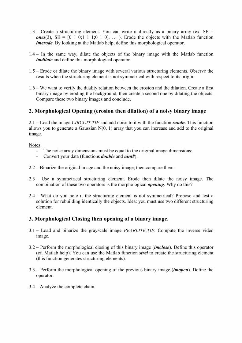
1.3 – Create a structuring element. You can write it directly as a binary array (ex. SE =
ones(3), SE = [0 1 0;1 1 1;0 1 0], … ). Erode the objects with the Matlab function
imerode. By looking at the Matlab help, define this morphological operator.
1.4 – In the same way, dilate the objects of the binary image with the Matlab function
imdilate and define this morphological operator.
1.5 – Erode or dilate the binary image with several various structuring elements. Observe the
results when the structuring element is not symmetrical with respect to its origin.
1.6 – We want to verify the duality relation between the erosion and the dilation. Create a first
binary image by eroding the background, then create a second one by dilating the objects.
Compare these two binary images and conclude.
2. Morphological Opening (erosion then dilation) of a noisy binary image
2.1 – Load the image CIRCUIT.TIF and add noise to it with the function randn. This function
allows you to generate a Gaussian N(0, 1) array that you can increase and add to the original
image.
Notes:
- The noise array dimensions must be equal to the original image dimensions;
- Convert your data (functions double and uint8).
2.2 – Binarize the original image and the noisy image, then compare them.
2.3 – Use a symmetrical structuring element. Erode then dilate the noisy image. The
combination of these two operators is the morphological opening. Why do this?
2.4 – What do you note if the structuring element is not symmetrical? Propose and test a
solution for rebuilding identically the objects. Idea: you must use two different structuring
element.
3. Morphological Closing then opening of a binary image.
3.1 – Load and binarize the grayscale image PEARLITE.TIF. Compute the inverse video
image.
3.2 – Perform the morphological closing of this binary image (imclose). Define this operator
(cf. Matlab help). You can use the Matlab function strel to create the structuring element
(this function generates structuring elements).
3.3 – Perform the morphological opening of the previous binary image (imopen). Define the
operator.
3.4 – Analyze the complete chain.
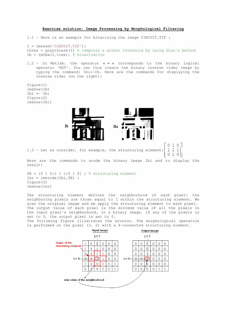
Exercise solution: Image Processing by Morphologica l Filtering 1.1 – Here is an example for binarizing the image CIRCUIT.TIF : I = imread( 'CIRCUIT.TIF' ); thres = graythresh(I) % computes a global threshold by using Otsu’s metho d Ib = im2bw(I,tres); % binarization 1.2 – In Matlab, the operator « ~ » corresponds to the binary logical
operator ‘NOT’. You can thus create the binary inve rse video image by typing the command: Ibi=~Ib. Here are the commands for displaying the inverse video (on the right):
figure(1) imshow(Ib) Ibi =~ Ib; figure(2) imshow(Ibi)
1.3 – Let us consider, for example, the structuring element:
010111010
Here are the commands to erode the binary image Ibi and to display the result: SE = [0 1 0;1 1 1;0 1 0] ; % structuring element Ier = imerode(Ibi,SE) ; figure(3) imshow(Ier) The structuring element defines the neighborhood of each pixel: the neighboring pixels are those equal to 1 within the structuring element. We scan the original image and we apply the structurin g element to each pixel. The output value of each pixel is the minimum value of all the pixels in the input pixel's neighborhood. In a binary image, if any of the pixels is set to 0, the output pixel is set to 0. The following figure illustrates the erosion. The m orphological operation is performed on the pixel (3, 2) with a 4-connected structuring element.

Here is the eroded image:
The erosion removes the white pixels which are isol ated in the background and erodes the edges of the objects within the imag e CIRCUIT. 1.4 – Here are the commands to dilate the binary im age Ibi and for
displaying the result: Idi = imdilate(Ibi,SE) ; figure(4) imshow(Idi) The output value of each pixel is the maximum value of all the pixels in the input pixel's neighborhood. In a binary image, if any of the pixels is set to 1, the output pixel is set to 1. The following figure illustrates the dilation. The morphological operation is performed on the pixel (2, 4) with a 4-connected structuring element.
Here is the image obtained:
The dilation removes the holes which are isolated i n the objects and dilates the object edges by taking account of the s tructuring element shape.
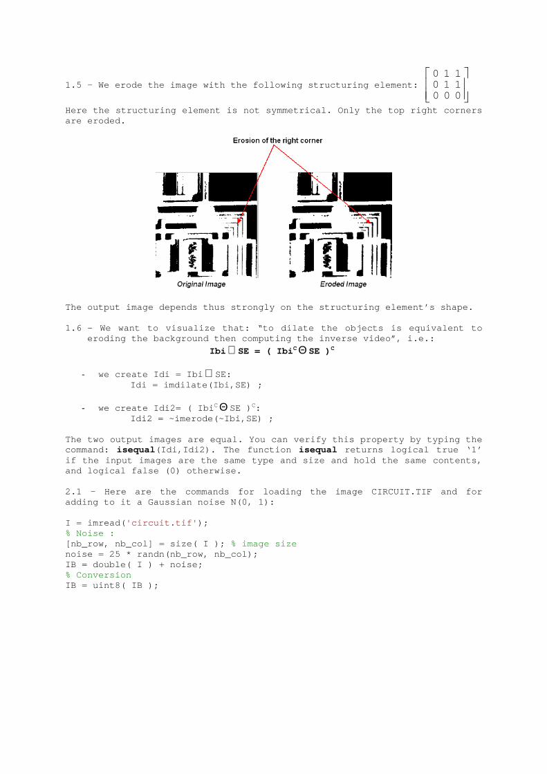
1.5 – We erode the image with the following structu ring element:
000110110
Here the structuring element is not symmetrical. On ly the top right corners are eroded.
The output image depends thus strongly on the struc turing element’s shape. 1.6 – We want to visualize that: “to dilate the obj ects is equivalent to
eroding the background then computing the inverse v ideo”, i.e.:
Ibi ⊕ SE = ( Ibi CΘ SE ) C
- we create Idi = Ibi ⊕ SE: Idi = imdilate(Ibi,SE) ;
- we create Idi2= ( Ibi CΘ SE ) C: Idi2 = ~imerode(~Ibi,SE) ;
The two output images are equal. You can verify thi s property by typing the command: isequal(Idi,Idi2). The function isequal returns logical true ‘1’ if the input images are the same type and size and hold the same contents, and logical false (0) otherwise. 2.1 – Here are the commands for loading the image CIRCUIT.TIF and for adding to it a Gaussian noise N(0, 1): I = imread( 'circuit.tif' ); % Noise : [nb_row, nb_col] = size( I ); % image size noise = 25 * randn(nb_row, nb_col); IB = double( I ) + noise; % Conversion IB = uint8( IB );
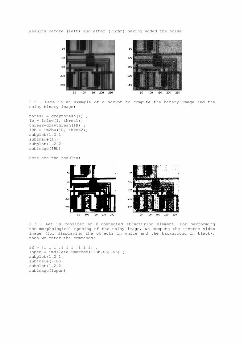
Results before (left) and after (right) having adde d the noise:
2.2 – Here is an example of a script to compute the binary image and the noisy binary image: thres1 = graythresh(I) ; Ib = im2bw(I, thres1); thres2=graythresh(IB) ; IBb = im2bw(IB, thres2); subplot(1,2,1) subimage(Ib) subplot(1,2,2) subimage(IBb) Here are the results:
2.3 – Let us consider an 8-connected structuring el ement. For performing the morphological opening of the noisy image, we co mpute the inverse video image (for displaying the objects in white and the background in black), then we enter the commands: SE = [1 1 1 ;1 1 1 ;1 1 1] ; Iopen = imdilate(imerode(~IBb,SE),SE) ; subplot(1,2,1) subimage(~IBb) subplot(1,2,2) subimage(Iopen)

Here are the images displayed:
In this case, the interest of such a operation is t o initially erode the objects of the image for removing the isolated pixe ls which correspond to the noise. The result is then dilated to resize the objects. The noise is thus reduced. 2.4 – If the structuring element is not symmetrical , the erosion reduces the noise again (isolated pixels in the background) . For resizing the original objects, we perform dilation by the same s tructuring element.
♦ Warning : You must be really careful when you perform the dil ation:
X⊕ B = { p ∈S, so that pB ∩ X ≠ ∅}
The dilation of an object X by a structuring elemen t B is defined by the symmetrical structuring element. The result is the set of poin ts P(p) so that the translated symmetrical structuring element has a non-null intersection with the object. Let us consider, for example, a non-symmetrical str ucturing element:
000011011
The top left corner is eroded:
For resizing the object, we want to perform dilatio n. Let us consider that the definition of the dilation is not based on the
symmetrical structuring element: X ⊕ B = { p ∈S, so that B p ∩ X ≠ ∅}. Be careful: this definition is entirely false and a ims to show you a classical mistake, made when you don’t consider the symmetrical structuring element.

Here is the result obtained with the bad definition of the dilation. We visualize that the lower right corner is dilated wh ereas we wanted to dilate the upper left corner:
To rebuild the original top left corner, it is nece ssary to use the
structuring element:
110110000
which is symmetrical to the original
structuring element. In order to perform morphological openings and clos ings which guarantee the reconstruction of the objects, the definition of the dilation is based on the symmetrical structuring element . In the special case of a morphological opening by a symmetrical structuring element, the p roblem does not exist obviously. Here is an example of a script for performing the m orphological opening of the noisy binary image Circuit by a non-symmetrical structuring element: SE1 = [1 1 0 ;1 1 0 ;0 0 0] SE2 = [0 0 0 ;0 1 1 ;0 1 1] Iouv = imdilate(imerode(~IBb,SE1),SE2) ; Here are the results:
The noise is reduced and the output image’s objects are the same size as the input image’s objects.

3.1 – Here are the commands for loading, binarizing and computing the inverse video of the grayscale image Pearlite.tif: I = imread( ‘pearlite.tif’ ); L = graythresh(I) I = ~im2bw(I,L); 3.2 – For performing the morphological closing of t his image, we create a structuring element with the Matlab function strel: SE = strel( 'disk' , 6) Here is the result you can visualize in the command window:
The morphological closing of the image is computed by typing the command: Iclos = imclose(I,SE); Here is displayed the result:
The morphological closing smoothes the object borde rs, it merges together the small features in the image that are close toge ther and the narrow channels and small holes are thus filled up.

3.3 – For performing the morphological opening of t he previous image, we use the Matlab function imopen: Im = imopen(Iclos,SE); We obtain the following result:
The morphological opening smoothes the object borde rs and removes small objects while preserving the shape and size of larg er objects in the original binary image. 3.5 – The combination of the morphological closing with the morphological opening allows you to extract the large objects wit hin the binary image: the image is segmented. These two operators are typ ically used for smoothing the object edges, for removing objects or for filling holes. The structuring element shape must be chosen according to the size and the shape of the objects that we want to modify.

Morphological Filtering of grayscale images
Direct extension of binary morphology through the notion of shadow (or sub-graph) of the image function
• gray level « f » of a pixel P : f (m, n) where (m, n) is the affix of P
example ( case of 1-D signal ):
Definitions:
• sub-graph « U ( f ) » : U ( f ) = { (m, n, l), l∈R, so that: l ≤
f (m, n) }• reconstruction T of the image « f » from its sub-graph U ( f ):
f (m, n) = T [ U ( f ) ] = Supl { l so that (m, n, l) ∈
U ( f ) }
n
f ( n ) U ( f )

Erosion of a grayscale image
The erosion (noted Ө ) of a grayscale image « f » by the structuring element « B » is defined from the sub-graph notions:
min68 , 90 , 91 , 95 , 151
( f Ө
B ) (P) = 68
• f Ө
B = T [ Y ] = Supl { l so that (m, n, l) ∈
Y }• Y = U ( f ) Ө
U ( B )
Commonly we choose a plane structuring element which has zero value
on its support( f Ө
B ) (P) = Min { values of the P-neighborhood }
n115 91 7795 68 9055 151 210
example :
m
Original Image
Ө
Structuring Element(4-connected)
∗- Classified values of the
neighborhood :--
-

Dilation of a grayscale image
The dilation (noted ⊕ ) is also defined from sub-graph notions:
max
55 , 68 , 77 , 90 , 91 , 95 , 115 , 151 , 210
( f ⊕
B ) (P) = 210
• f ⊕
B = T [ Y ] = Supl { l so that (m, n, l) ∈
Y }
• Y = U ( f ) ⊕
U ( B )
If you consider a plane structuring element which has zero valueon its support:
( f ⊕
B ) (P) = Max { values of the P-neighborhood }
n115 91 7795 68 9055 151 210
example:
m
Original Image
⊕
Structuring Element(8-connected)
∗Classified values of the
neighborhood:- - -
---
--

Examples of morphological filtering(full 3×3 structuring element)
Original image
Erosion
Dilation
The erosion of grayscale images decreases the luminance value of the pixels which have low- intensity neighborhoods
Note:
The dilation of grayscale images increases the luminance value of the pixels which have high-intensity neighborhoods
Observation:

Exercise Chapter 4 – Morphological Filtering of grayscale images
In this exercise we want to extend the morphological filtering to the grayscale images. Load
the grayscale image CAMERAMAN.TIF et update the path list in the path browser.
♦ Note: we consider for the binary images that the objects are set to 1 and the background is set to 0, therefore we must often inverse the binary natural images. In the case of the grayscale
natural images, the objects are rather dark and the background is rather white. We perform
also an inverse video transformation with the Matlab function imcomplement (type help
imcomplement fore more information). We obtain thus white objects and a dark background.
Morphological filtering of grayscale images
1 – Erode the image Cameraman.tif (imerode) by the following structuring element:
SE=strel('ball',5,5).
Display the result and compare with the original image. Define this operator thanks to the
Matlab Image Processing toolbox.
2 – In the same way, dilate the original image Cameraman.tif (imdilate) by the same
structuring element. Display the result and compare with the original image. Use the Matlab
Image Processing toolbox for defining this operator.
3 – Perform a morphological opening then a morphological closing of the original image
Cameraman.tif. Observe and interpret the obtained results.

Exercise solution: Morphological filtering of grayscale images 1 – Here are the commands for eroding the original image and for comparing the result with the original image: % Image loading I = imread( ‘cameraman.tif’ ) ; Ic = imcomplement(I); % inverse video of original image figure(1) subplot(1,2,1) subimage(I) title( ‘Original image’ ); subplot(1,2,2) subimage(Ic) title( ‘Original image (inverse video)’ ); % Erosion SE = strel('ball',5,5) % structuring element Ierod = imerode(Ic,SE); figure(2) subplot(1,2,1) subimage(Ierod) title( ‘Eroded image (inverse video)’ ); % Display the eroded grayscale image without invers e video effect subplot(1,2,2) subimage(imcomplement(Ierod)) title( ‘Eroded image’ ); Here are the results:
The erosion of grayscale images decreases the lumin ance value of the pixels which have low-intensity neighborhood (you can visu alize this phenomenon on

the images with inverse video effect). The neighbor hood depends on the structuring element. The pixels of the input image are scanned: each pixel is considered as the origin of the structuring elem ent (by translation). The output value of each pixel is then equal to the minimal value of its neighboring pixels. 2 – Here are the commands for dilating the original image and for comparing the result with the original image: % Dilation figure(3) Idilat = imdilate(Ic,SE); subplot(1,2,1) subimage(Idilat) title( ‘Dilated image (inverse video)’ ); subplot(1,2,2) subimage(imcomplement(Idilat)) title( ‘Dilated image’ ); We display the following results:
The dilation of grayscale images increases the lumi nance value of the pixels which have high-intensity neighborhood (you can visualize this phenomenon, on the images with inverse video effect ). The output value of each pixel is the maximal value of all its neighboring pixels.

3 – Here is an example of a script for performing t he morphological opening and for comparing the result with the original imag e: % Morphological opening figure(4) Iopen = imopen(Ic,SE); subplot(1,2,1) subimage(Iopen) title( ‘Morphological Opening (inverse video)’ ); subplot(1,2,2) subimage(imcomplement(Iopen)) title( ‘Morphological Opening’ ); Here are the results:
The morphological opening consists of erosion follo wed by the dilation of the original grayscale image. The morphological ope ning removes the white pixels which are isolated and smoothes the contours . We also visualize a segmentation of the objects within the image. Here is an example of a script for performing the m orphological closing: % Morphological closing figure(5) Iclose = imclose(Ic,SE); subplot(1,2,1) subimage(Iclose) title( ‘Morphological Closing (inverse video)’ ); subplot(1,2,2) subimage(imcomplement(Iclose)) title( ‘Morphological Closing’ );

Here are the images displayed:
The morphological closing consists of dilation foll owed by the erosion of the original grayscale image. The morphological clo sing removes the dark pixels which are isolated and smoothes the contours .

Chapter 4 – Non-linear Filtering
TEST
Exercise 1:
We want to perform several different filters for processing the following 5 × 5 image:
This image is a small portion of the original image “Boats” and contains a part of the fishing
boat’s boom. Here is the 5 × 5 matrix which contains the luminance values of this portion:
175 150 114 86 79
156 119 91 80 113
132 93 80 96 174
96 85 87 165 193
87 82 153 192 194
We do not take account of the boundary effects and we consider only the results obtained by
filtering of the 3 × 3 central pixels:
X X X X X
X ? ? ? X
X ? ? ? X
X ? ? ? X
X X X X X

Fill this matrix for each of the following cases:
- median filtering using the full 3×3 neighborhood, - median filtering using the 5-pixel cross-shaped neighborhood,
- erosion by a full 3×3 structuring element, - dilation by a full 3×3 structuring element, - morphological closing by a 5-pixel cross-shaped structuring element..
Exercise 2:
In Matlab, create the functions for dilating and for eroding an image (do not take account of
the boundary distortions). These two functions have two optional inputs: the original image
that we want to filter and the structuring element. The structuring element’s size will be less
than or equal to 3 × 3.
♦ Examples:
By using your two new functions, create the functions for performing the morphological
closing and the morphological opening.
Test your four functions by processing the image “Boats”. Compare the results with the
results that you obtain with the Matlab functions imdilate, imerode, imclose, and imopen.