Embed Size (px)
Citation preview
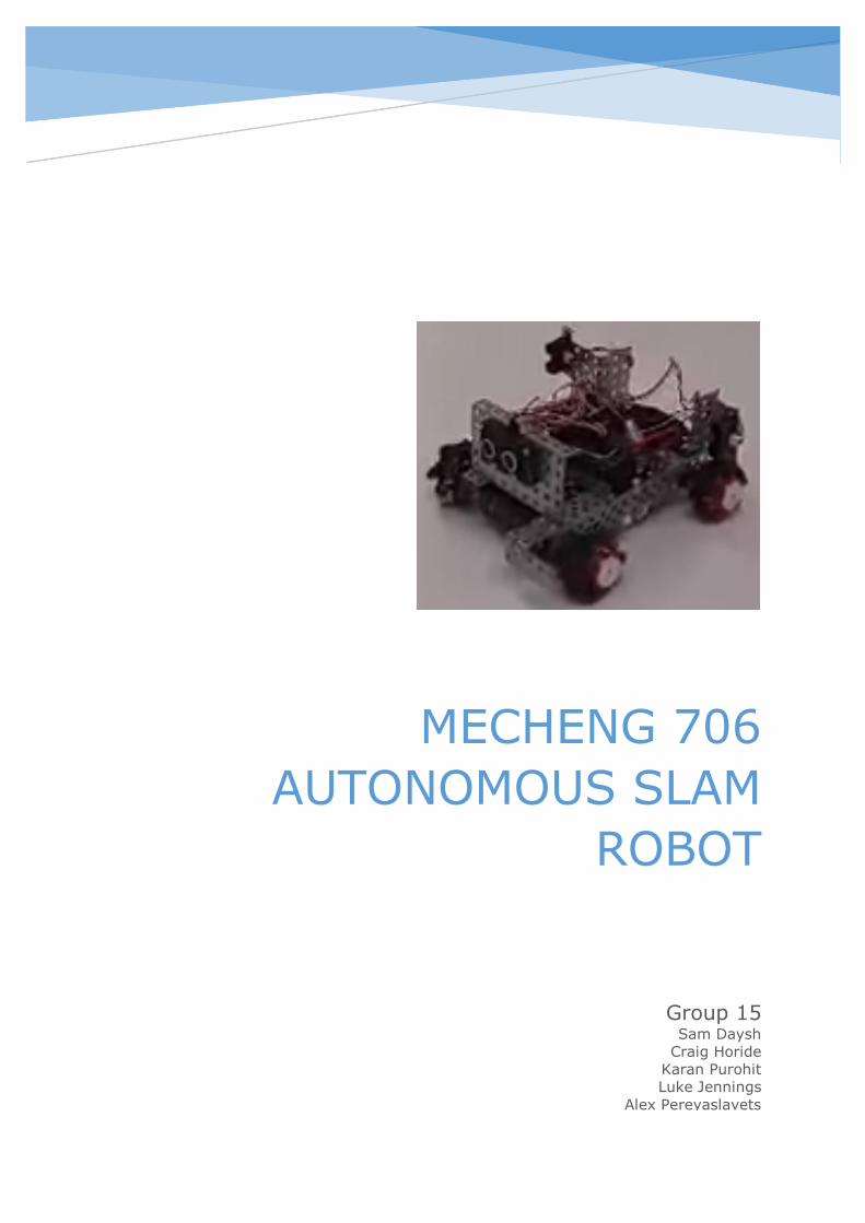
MECHENG 706
AUTONOMOUS SLAM
ROBOT
Group 15 Sam Daysh
Craig Horide
Karan Purohit
Luke Jennings
Alex Pereyaslavets
i
Executive Summary
The task given was to create an autonomous SLAM robot to cover an area, avoid
obstacles and map the path taken. To achieve this, each sensor was calibrated
and the limitations were found. Optimal path planning was considered and an
inwards spiral was agreed upon. Sensor limitations and the desired route
requirements were taken into account and a sensor arrangement was designed. A
finite state machine was created to realise the robot’s movement. The software
was constructed and tested before to ensure each state in the finite state machine
was working and performing as intended before entering its next state. In the end,
the robot attempted to cover the area quickly and avoid obstacles, however it was
not successful on the day. An attempted implementation of the map of the
environment was also done.
ii
Table of Contents
Executive Summary .................................................................................... i
Table of Figures ........................................................................................ iv
1. Introduction .......................................................................................... 1
1.1 Problem Description ........................................................................... 1
1.2 Problem Specification ......................................................................... 1
2. Sensors and Calibration .......................................................................... 2
2.1 Arduino Mega 2560 ............................................................................ 2
2.2 SHARP Infrared Sensors ..................................................................... 2
2.3 HC-SR04 ITead Studio Sonar .............................................................. 4
2.4 InvenSense MPU ................................................................................ 4
2.5 Sensor Placement .............................................................................. 5
3. Motion and Movement of the Robot .......................................................... 7
3.1 Mecanum Wheels ............................................................................... 7
3.2 Speed and Aligning ............................................................................ 8
3.3 Rotating vs Strafing ........................................................................... 8
3.4 Path Planning .................................................................................... 9
3.4.1 Zig-Zag Method ........................................................................... 9
3.4.2 Outward Spiralling ........................................................................ 9
3.4.3 Inward Spiralling ........................................................................ 10
3.4.4 Full SLAM .................................................................................. 10
4. Software ............................................................................................. 12
4.1. Interface Library ............................................................................. 12
4.2 General Functions ............................................................................ 12
4.2.1 Millis ......................................................................................... 12
4.2.2 Ninety Turn ............................................................................... 12
4.2.2 Scanning ................................................................................... 13
4.2.4 Get Sensor Data ........................................................................ 13
4.2.5 Display Sensor Readings ............................................................. 13
4.2.6 Align to wall .............................................................................. 14
4.3 Finite State Machine ......................................................................... 14
4.3.1 Initialisation .............................................................................. 15
4.3.2 Initial Wall Find .......................................................................... 15
4.3.3 Moving to Wall ........................................................................... 16
iii
4.3.4 Aligning to Wall .......................................................................... 16
4.3.5 Moving to Corner ....................................................................... 16
4.3.6 Running .................................................................................... 16
4.3.8 Object Detected ......................................................................... 17
4.3.9 Object Detected Forwards ........................................................... 18
4.3.10 Object Passing ......................................................................... 18
4.3.11 Re-adjusting ............................................................................ 19
4.3.12 Stopped .................................................................................. 20
4.4 Mapping ............................................................................................ 20
5. Testing and Results .............................................................................. 23
6. Discussion, Limitations and Improvements .............................................. 24
6.1 IR Sensors ...................................................................................... 24
6.2 Number of Sensors .......................................................................... 24
6.3 Motors ............................................................................................ 24
6.4 Limited Movement Directions ............................................................ 24
6.5 Servo Motor Usage .......................................................................... 25
6.6 MPU for Turning............................................................................... 25
6.7 PID Control ..................................................................................... 25
6.8 Fuzzy Logic ..................................................................................... 25
6.9 Active SLAM .................................................................................... 26
6.10 Finite State Machine ....................................................................... 26
7. Conclusion ........................................................................................... 26
Appendices............................................................................................. A-1
Appendix I – Sonar Mount Drawing ........................................................... A-2
Appendix II – MPU Mount Drawing ............................................................ A-3
Appendix III – Ninety Turn Code ............................................................... A-4
Appendix IV – Scanning Code ................................................................... A-5
Appendix V – Get Sensor Data Code .......................................................... A-6
Appendix VI – Align to Wall Code .............................................................. A-7
Appendix VII – Finite State Machine .......................................................... A-8
iv
Table of Figures
Figure 1 - Arduino Mega 2560 ..................................................................... 2
Figure 2 - Medium Range Sensor ................................................................. 2
Figure 3 - Long Range Sensor ...................................................................... 2
Figure 4 - Long Range Measure versus Real Values ........................................ 3
Figure 5 - Medium Range Measure versus Real Values .................................... 3
Figure 6 - Sonar Range Finder ..................................................................... 4
Figure 7 - MPU 9150 ................................................................................... 4
Figure 8 - First Arrangement of Sensors ........................................................ 5
Figure 9 - Second Arrangement of Sensors .................................................... 5
Figure 10 - Final Arrangement of Sensors ..................................................... 6
Figure 11 - Basic Control System ................................................................. 7
Figure 12 - Mecanum Wheels Kinematics ...................................................... 7
Figure 13 - Zig-Zag Method ......................................................................... 9
Figure 14 - Zig-Zag Method with Obstacles ................................................... 9
Figure 15 - Outward Spiral Method ............................................................. 10
Figure 16 - Outward Spiral Method with Obstacles ........................................ 10
Figure 17 - Inward Spiral Method ............................................................... 10
Figure 18 - Inward Spiral Method with Obstacles .......................................... 10
Figure 19 - Scanning Function ................................................................... 13
Figure 20 - Basic Finite State Machine ........................................................ 14
Figure 21 - Initialisation Sequence ............................................................. 15
Figure 22 - Object Detected ...................................................................... 17
Figure 23 - Robot Strafing Left in Object Detected ....................................... 17
Figure 24 - Object Detected Forwards ......................................................... 18
Figure 25 - Object Passing ........................................................................ 18
Figure 26 - Object Re-adjusting ................................................................. 19
Figure 27 - Object Continuing on Path ........................................................ 19
Figure 28 - Final Finite State Machine ......................................................... 20
Figure 29 - Mapping Implementation .......................................................... 21
Figure 30 - On Day Results ....................................................................... 23
1
1. Introduction
Simultaneous Localisation and Mapping is a difficult problem which is key to
successful and effective autonomous robotics and entails generating a map of an
unknown environment while tracking the pose of the robot within it. The difficulty
lies in the circular dependency of localisation requiring a map to localise against,
and mapping requiring a known pose to accurately generate a map. If a SLAM
algorithm is successfully implemented, it can be used for many autonomous
robotics applications such as vacuum cleaning, generating maps of environments
too small for humans, and reef monitoring underwater.
1.1 Problem Description
With the intention of autonomous vacuum cleaning, the task given was to design
and create an autonomous SLAM robot using given sensors and chassis with
mecanum wheels. The robot was to navigate around an unknown area, whilst
avoiding an unknown number of obstacles of unknown size. It was also required
to output the map of the area and the path traversed. The success of the robot’s
operation would be measured by how fast the robot covers the area, how well the
robot avoids obstacles, and its mapping and localisation capabilities.
1.2 Problem Specification
The robot was given mecanum wheels for movement using VEX 2-wire 393
motors, a selection of range finding sensors including an array of infrared and a
sonar, an MPU-9150, and an Arduino Mega 2560 controller board for memory and
logic control. It also contained a Bluetooth module to communicate with a
computer for troubleshooting and mapping capabilities.
2
2. Sensors and Calibration
2.1 Arduino Mega 2560
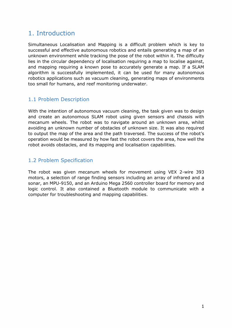
The Arduino Mega 2560, shown in Figure 1, is a microcontroller board, with 54
digital I/O pins, 16 analogue inputs and its own 16 MHz crystal oscillator. It has
an 8 KB SRAM memory which is used for global variables and a 256 KB flash
memory. It is powered by a battery through USB port. It proves effective for the
purposes of SLAM on a small scale - if a more computationally difficult SLAM
algorithm was required, or a higher resolution map, it would not be sufficient.
2.2 SHARP Infrared Sensors
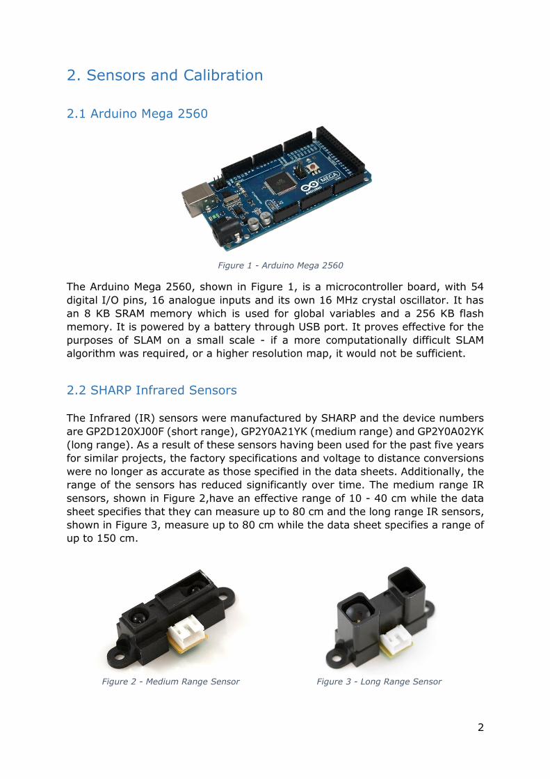
The Infrared (IR) sensors were manufactured by SHARP and the device numbers
are GP2D120XJ00F (short range), GP2Y0A21YK (medium range) and GP2Y0A02YK
(long range). As a result of these sensors having been used for the past five years
for similar projects, the factory specifications and voltage to distance conversions
were no longer as accurate as those specified in the data sheets. Additionally, the
range of the sensors has reduced significantly over time. The medium range IR
sensors, shown in Figure 2,have an effective range of 10 - 40 cm while the data
sheet specifies that they can measure up to 80 cm and the long range IR sensors,
shown in Figure 3, measure up to 80 cm while the data sheet specifies a range of
up to 150 cm.
Figure 2 - Medium Range Sensor
Figure 3 - Long Range Sensor
Figure 1 - Arduino Mega 2560
3
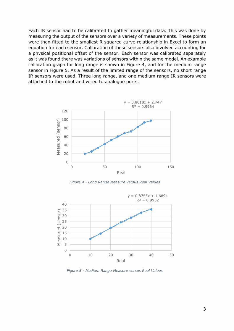
Each IR sensor had to be calibrated to gather meaningful data. This was done by
measuring the output of the sensors over a variety of measurements. These points
were then fitted to the smallest R squared curve relationship in Excel to form an
equation for each sensor. Calibration of these sensors also involved accounting for
a physical positional offset of the sensor. Each sensor was calibrated separately
as it was found there was variations of sensors within the same model. An example
calibration graph for long range is shown in Figure 4, and for the medium range
sensor in Figure 5. As a result of the limited range of the sensors, no short range
IR sensors were used. Three long range, and one medium range IR sensors were
attached to the robot and wired to analogue ports.
Figure 4 - Long Range Measure versus Real Values
Figure 5 - Medium Range Measure versus Real Values
y = 0.8018x + 2.747
R² = 0.9964
0
20
40
60
80
100
120
0 50 100 150
Measure
d (
sensor)
Real
y = 0.8755x + 1.6894
R² = 0.9952
0
5
10
15
20
25
30
35
40
0 10 20 30 40 50
Measure
d (
sensor)
Real
4
2.3 HC-SR04 ITead Studio Sonar
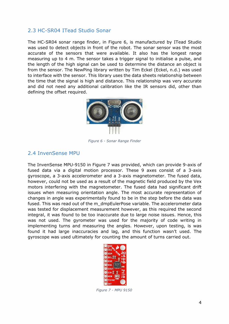
The HC-SR04 sonar range finder, in Figure 6, is manufactured by ITead Studio
was used to detect objects in front of the robot. The sonar sensor was the most
accurate of the sensors that were available. It also has the longest range
measuring up to 4 m. The sensor takes a trigger signal to initialise a pulse, and
the length of the high signal can be used to determine the distance an object is
from the sensor. The NewPing library written by Tim Eckel (Eckel, n.d.) was used
to interface with the sensor. This library uses the data sheets relationship between
the time that the signal is high and distance. This relationship was very accurate
and did not need any additional calibration like the IR sensors did, other than
defining the offset required.
2.4 InvenSense MPU
The InvenSense MPU-9150 in Figure 7 was provided, which can provide 9-axis of
fused data via a digital motion processor. These 9 axes consist of a 3-axis
gyroscope, a 3-axis accelerometer and a 3-axis magnetometer. The fused data,
however, could not be used as a result of the magnetic field produced by the Vex
motors interfering with the magnetometer. The fused data had significant drift
issues when measuring orientation angle. The most accurate representation of
changes in angle was experimentally found to be in the step before the data was
fused. This was read out of the m_dmpEulerPose variable. The accelerometer data
was tested for displacement measurement however, as this required the second
integral, it was found to be too inaccurate due to large noise issues. Hence, this
was not used. The gyrometer was used for the majority of code writing in
implementing turns and measuring the angles. However, upon testing, is was
found it had large inaccuracies and lag, and this function wasn’t used. The
gyroscope was used ultimately for counting the amount of turns carried out.
Figure 6 - Sonar Range Finder
Figure 7 - MPU 9150
5
2.5 Sensor Placement
There were several different sensor position concepts, which had positives and
negatives, and ultimately the sensor placement was decided by being the most
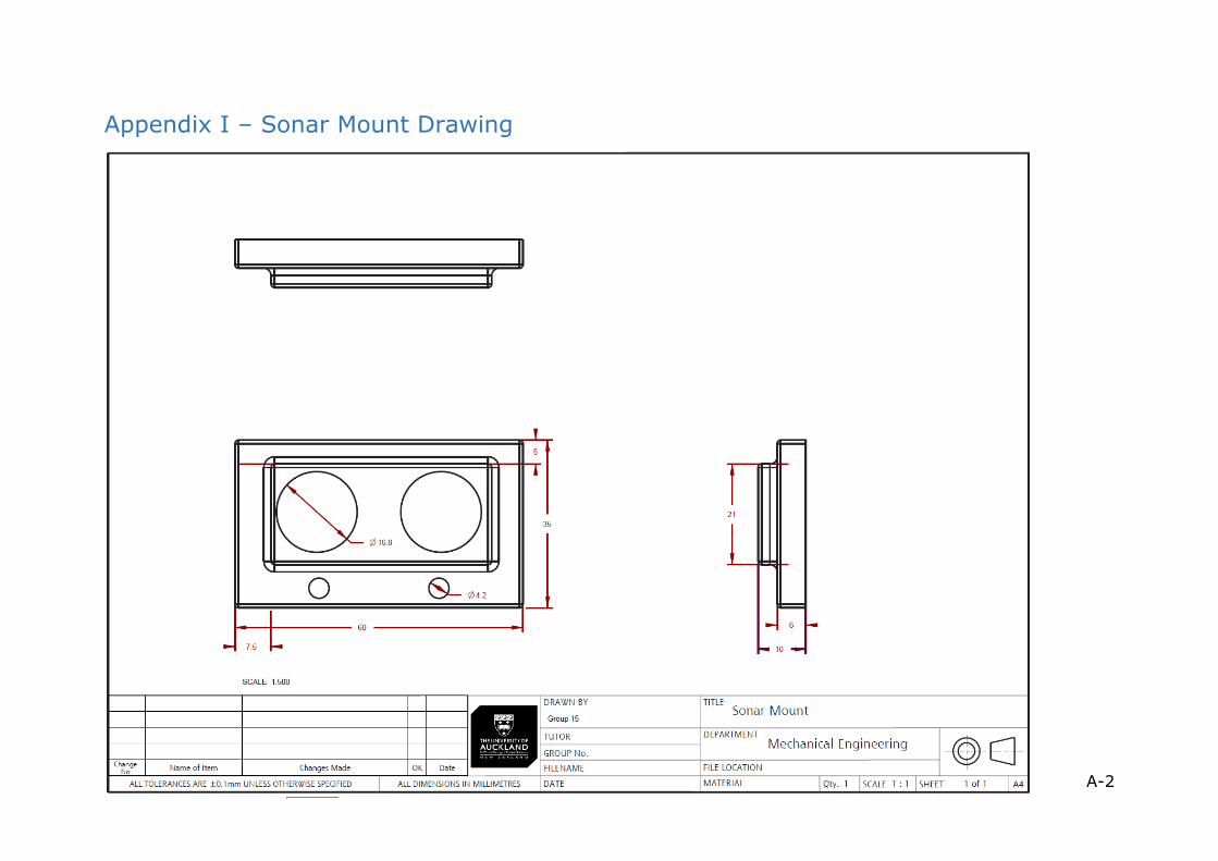
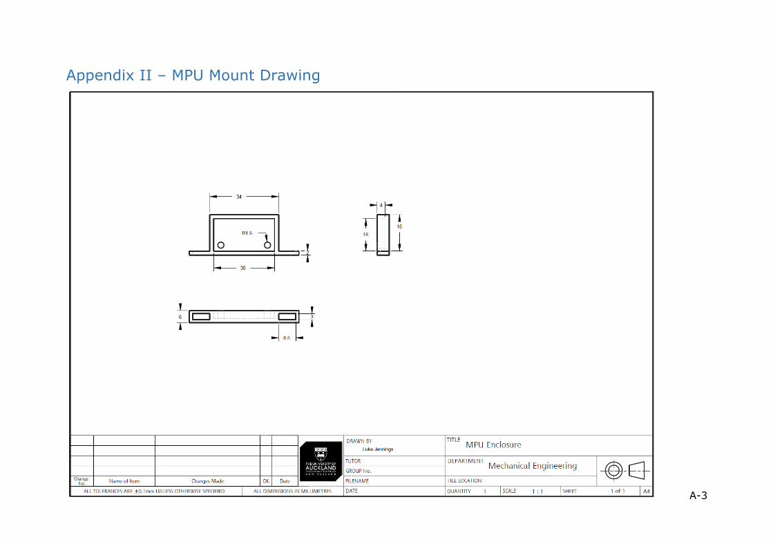
practical. The sonar was always placed in the centre facing forward, and the MPU
vertical behind the pins. The mounting structure drawings are attached in
Appendices I and II. The changes were due to the IR sensor usage and effective
range. All sensors are attached using VEX Robotics components which offer stable
and standard sizes.
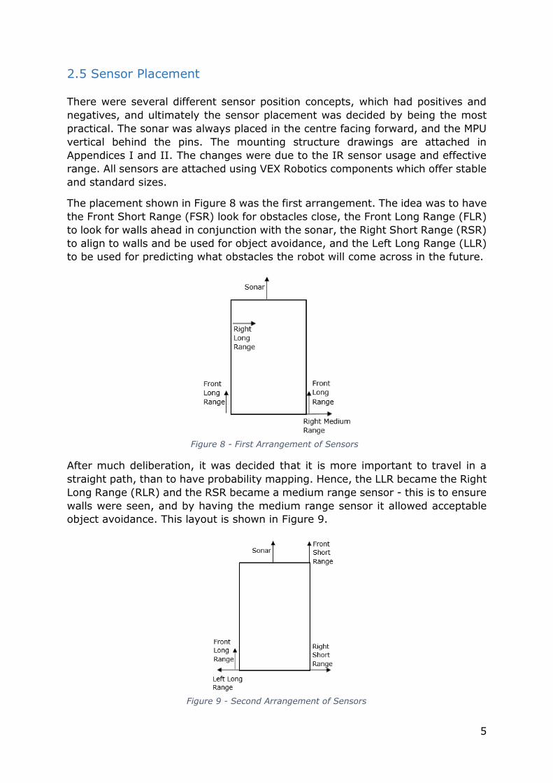
The placement shown in Figure 8 was the first arrangement. The idea was to have
the Front Short Range (FSR) look for obstacles close, the Front Long Range (FLR)
to look for walls ahead in conjunction with the sonar, the Right Short Range (RSR)
to align to walls and be used for object avoidance, and the Left Long Range (LLR)
to be used for predicting what obstacles the robot will come across in the future.
After much deliberation, it was decided that it is more important to travel in a
straight path, than to have probability mapping. Hence, the LLR became the Right
Long Range (RLR) and the RSR became a medium range sensor - this is to ensure
walls were seen, and by having the medium range sensor it allowed acceptable
object avoidance. This layout is shown in Figure 9.
Figure 8 - First Arrangement of Sensors
Figure 9 - Second Arrangement of Sensors
6
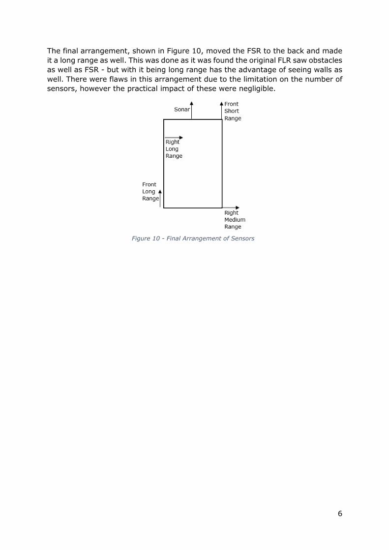
The final arrangement, shown in Figure 10, moved the FSR to the back and made
it a long range as well. This was done as it was found the original FLR saw obstacles
as well as FSR - but with it being long range has the advantage of seeing walls as
well. There were flaws in this arrangement due to the limitation on the number of
sensors, however the practical impact of these were negligible.
Figure 10 - Final Arrangement of Sensors
7
3. Motion and Movement of the Robot
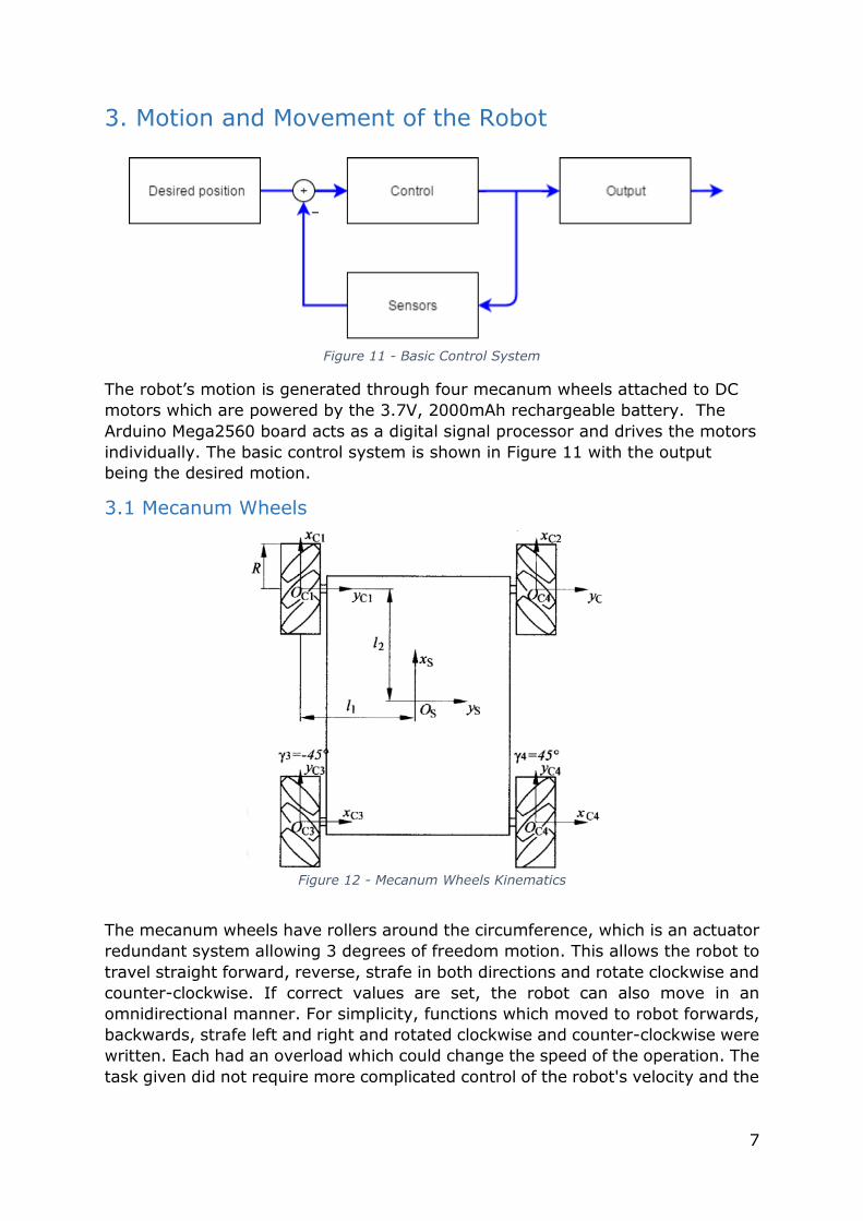
The robot’s motion is generated through four mecanum wheels attached to DC
motors which are powered by the 3.7V, 2000mAh rechargeable battery. The
Arduino Mega2560 board acts as a digital signal processor and drives the motors
individually. The basic control system is shown in Figure 11 with the output
being the desired motion.
3.1 Mecanum Wheels
The mecanum wheels have rollers around the circumference, which is an actuator
redundant system allowing 3 degrees of freedom motion. This allows the robot to
travel straight forward, reverse, strafe in both directions and rotate clockwise and
counter-clockwise. If correct values are set, the robot can also move in an
omnidirectional manner. For simplicity, functions which moved to robot forwards,
backwards, strafe left and right and rotated clockwise and counter-clockwise were
written. Each had an overload which could change the speed of the operation. The
task given did not require more complicated control of the robot's velocity and the
Figure 11 - Basic Control System
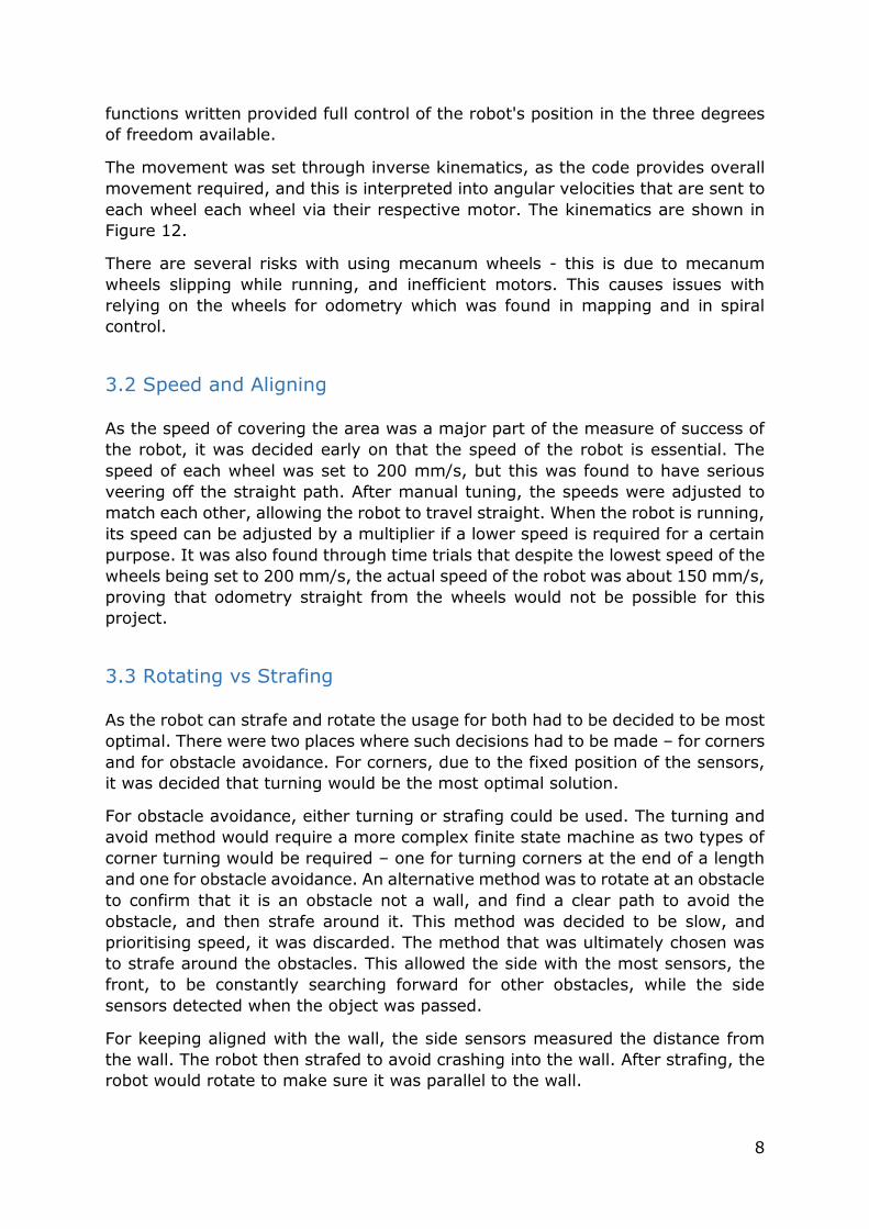
Figure 12 - Mecanum Wheels Kinematics
8
functions written provided full control of the robot's position in the three degrees
of freedom available.
The movement was set through inverse kinematics, as the code provides overall
movement required, and this is interpreted into angular velocities that are sent to
each wheel each wheel via their respective motor. The kinematics are shown in
Figure 12.
There are several risks with using mecanum wheels - this is due to mecanum
wheels slipping while running, and inefficient motors. This causes issues with
relying on the wheels for odometry which was found in mapping and in spiral
control.
3.2 Speed and Aligning
As the speed of covering the area was a major part of the measure of success of
the robot, it was decided early on that the speed of the robot is essential. The
speed of each wheel was set to 200 mm/s, but this was found to have serious
veering off the straight path. After manual tuning, the speeds were adjusted to
match each other, allowing the robot to travel straight. When the robot is running,
its speed can be adjusted by a multiplier if a lower speed is required for a certain
purpose. It was also found through time trials that despite the lowest speed of the
wheels being set to 200 mm/s, the actual speed of the robot was about 150 mm/s,
proving that odometry straight from the wheels would not be possible for this
project.
3.3 Rotating vs Strafing
As the robot can strafe and rotate the usage for both had to be decided to be most
optimal. There were two places where such decisions had to be made – for corners
and for obstacle avoidance. For corners, due to the fixed position of the sensors,
it was decided that turning would be the most optimal solution.
For obstacle avoidance, either turning or strafing could be used. The turning and
avoid method would require a more complex finite state machine as two types of
corner turning would be required – one for turning corners at the end of a length
and one for obstacle avoidance. An alternative method was to rotate at an obstacle
to confirm that it is an obstacle not a wall, and find a clear path to avoid the
obstacle, and then strafe around it. This method was decided to be slow, and
prioritising speed, it was discarded. The method that was ultimately chosen was
to strafe around the obstacles. This allowed the side with the most sensors, the
front, to be constantly searching forward for other obstacles, while the side
sensors detected when the object was passed.
For keeping aligned with the wall, the side sensors measured the distance from
the wall. The robot then strafed to avoid crashing into the wall. After strafing, the
robot would rotate to make sure it was parallel to the wall.
9
3.4 Path Planning
There are several ways that a robot can navigate through an environment and
each has its own benefits and weaknesses. The primary techniques that were
considered are described below.
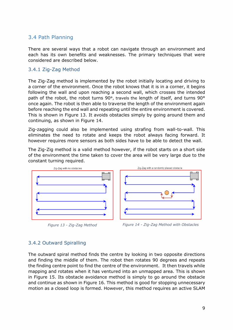
3.4.1 Zig-Zag Method
The Zig-Zag method is implemented by the robot initially locating and driving to
a corner of the environment. Once the robot knows that it is in a corner, it begins
following the wall and upon reaching a second wall, which crosses the intended
path of the robot, the robot turns 90°, travels the length of itself, and turns 90°
once again. The robot is then able to traverse the length of the environment again
before reaching the end wall and repeating until the entire environment is covered.
This is shown in Figure 13. It avoids obstacles simply by going around them and
continuing, as shown in Figure 14.
Zig-zagging could also be implemented using strafing from wall-to-wall. This
eliminates the need to rotate and keeps the robot always facing forward. It
however requires more sensors as both sides have to be able to detect the wall.
The Zig-Zig method is a valid method however, if the robot starts on a short side
of the environment the time taken to cover the area will be very large due to the
constant turning required.
Figure 13 - Zig-Zag Method
Figure 14 - Zig-Zag Method with Obstacles
3.4.2 Outward Spiralling
The outward spiral method finds the centre by looking in two opposite directions
and finding the middle of them. The robot then rotates 90 degrees and repeats
the finding centre point to find the centre of the environment. It then travels while
mapping and rotates when it has ventured into an unmapped area. This is shown
in Figure 15. Its obstacle avoidance method is simply to go around the obstacle
and continue as shown in Figure 16. This method is good for stopping unnecessary
motion as a closed loop is formed. However, this method requires an active SLAM

10
algorithm which is undesirable on an Arduino Mega, as it doesn’t have enough
memory to handle such a process.
Figure 15 - Outward Spiral Method
Figure 16 - Outward Spiral Method with
Obstacles
3.4.3 Inward Spiralling
Inward spiralling is another method for path planning, as shown in Figure 17. It is
realised by finding a wall and then following it to a corner. A variable is set which
specifies the distance from the wall that each trajectory runs from the wall parallel
to it. Once this variable is set the robot can begin travelling along a wall until it
reaches a corner, where it will turn 90°. The robot will repeat this until it
approaches the initial corner. From the initial corner onwards, the robot’s distance
from the wall is incremented. Avoiding obstacles is the same as previous methods
– simply avoid, and then continue as though there was no interference, as shown
in Figure 18. The inward spiralling method was the one that was ultimately chosen
as it allows the fastest area coverage with minimal processing power. For
simplicity’s sake, it was decided to use the right hand coordinate system, meaning
that the robot will always turn counter-clockwise.
Figure 17 - Inward Spiral Method
Figure 18 - Inward Spiral Method with
Obstacles
3.4.4 Full SLAM
A full SLAM method would be able to begin at any point in the map, assess the
area, and proceed to decide on the best path to take to map the area. This would
require high processing power due to the necessity of running more powerful
filtering algorithms, such as a Kalman or a Particle Filter. It would also not be
11
efficient in area coverage, as there would be parts of the environment that do not
require to be entered into to be mapped, yet the requirements of the project would
require the path to cover this area. Full SLAM is overly complicated for such a
simple project, hence, it was discarded as an option for path planning.
12
4. Software
Once the electronics were set up and basic logic developed the code had to be
implemented. The running code was written mostly in C with inbuilt Arduino
functions, and the map display was written in C#.
4.1. Interface Library
The interface library is a header file which encapsulates all of the robots interfacing
with the outside world. The intention was to create a series of functions which
would incorporate the calibration of the sensors and motor and simplify the tasks
of moving the robot into simple and intuitive functions. The library sets the relative
speed for the motors and has the calibrated relationships for each sensor, as well
as the input from the MPU.
4.2 General Functions
There are several functions that are used by the whole code. These are
described below.
4.2.1 Millis
All timing is done through the function millis(). This is an inbuilt function in Arduino
that runs from the beginning of the program and returns the time in milliseconds.
The timing is done through comparing the current output of millis() with previous
ones set for individual purposes. Once this exceeds the acceptable limit, which is
different for each state, the state runs. This allows other states, such as object
avoidance, to be triggered, without leaving the current functionality.
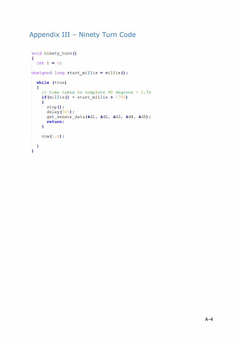
4.2.2 Ninety Turn
The ninety turn function is used whenever a 90o turn is required, which is at every
corner and in finding the initial corner. Initially, through the use of the MPU
gyrometer, this function would take the robot's initial angle, and turn until the
initial angle plus ninety degrees was achieved. This proved to be inaccurate due
to lag when updating the read angle and inconsistencies with readings in different
battery charge levels. The MPU based function was replaced by timing a 90o turn,
and providing a counter-clockwise rotation for that length of time. The final ninety
turn code is attached in Appendix III.
13
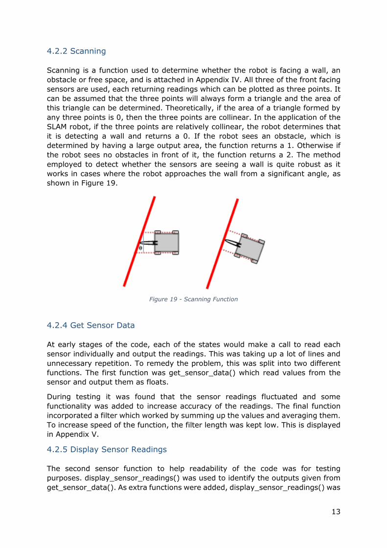
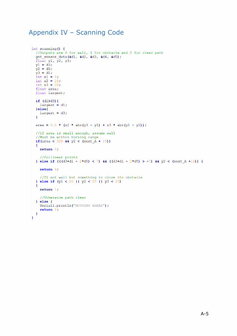
4.2.2 Scanning
Scanning is a function used to determine whether the robot is facing a wall, an
obstacle or free space, and is attached in Appendix IV. All three of the front facing
sensors are used, each returning readings which can be plotted as three points. It
can be assumed that the three points will always form a triangle and the area of
this triangle can be determined. Theoretically, if the area of a triangle formed by
any three points is 0, then the three points are collinear. In the application of the
SLAM robot, if the three points are relatively collinear, the robot determines that
it is detecting a wall and returns a 0. If the robot sees an obstacle, which is
determined by having a large output area, the function returns a 1. Otherwise if
the robot sees no obstacles in front of it, the function returns a 2. The method
employed to detect whether the sensors are seeing a wall is quite robust as it
works in cases where the robot approaches the wall from a significant angle, as
shown in Figure 19.
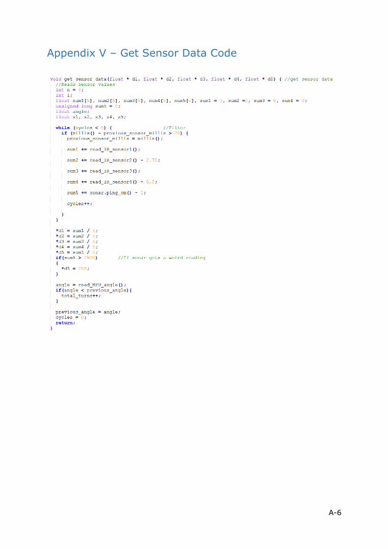
4.2.4 Get Sensor Data
At early stages of the code, each of the states would make a call to read each
sensor individually and output the readings. This was taking up a lot of lines and
unnecessary repetition. To remedy the problem, this was split into two different
functions. The first function was get_sensor_data() which read values from the
sensor and output them as floats.
During testing it was found that the sensor readings fluctuated and some
functionality was added to increase accuracy of the readings. The final function
incorporated a filter which worked by summing up the values and averaging them.
To increase speed of the function, the filter length was kept low. This is displayed
in Appendix V.
4.2.5 Display Sensor Readings
The second sensor function to help readability of the code was for testing
purposes. display_sensor_readings() was used to identify the outputs given from
get_sensor_data(). As extra functions were added, display_sensor_readings() was
Figure 19 - Scanning Function
14
also used to output certain values to the serial port, such as the difference between
two sensors.
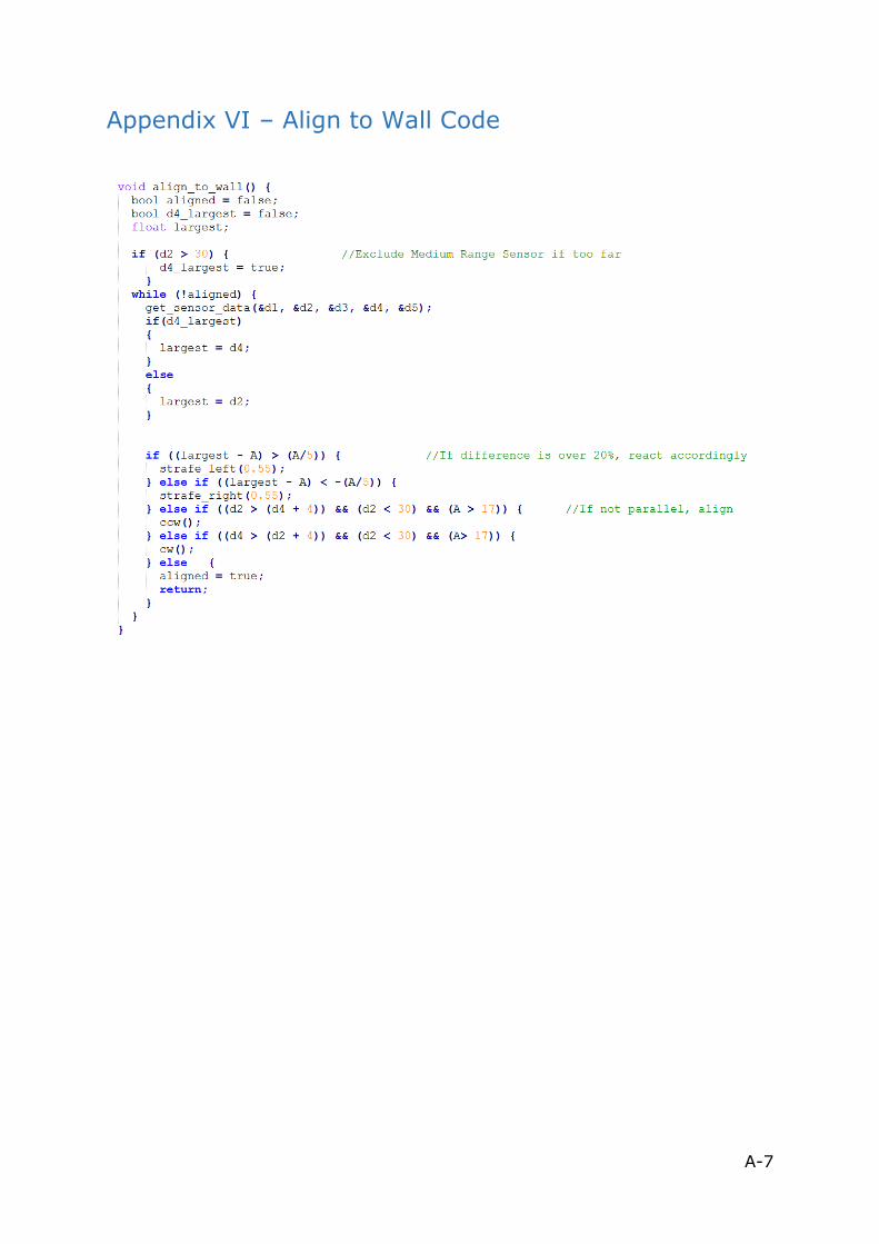
4.2.6 Align to wall
After testing the robot's movement, problems with accurate path following due to
drift and turning overshoots made it unable to correctly cover the given area. To
correct this, the function align_to_wall(), which is attached in Appendix VI, reads
the side sensors and adjusts the robot to realign itself parallel to the wall. When
the robot is in the centre this can prove to be problematic for the medium range
sensor, so only the long range data is effective. Thus, if the readings show that
the robot is far away from the wall, the function only makes choices based off the
long range sensor.
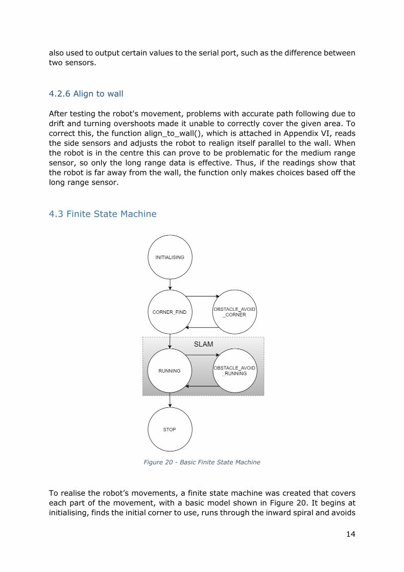
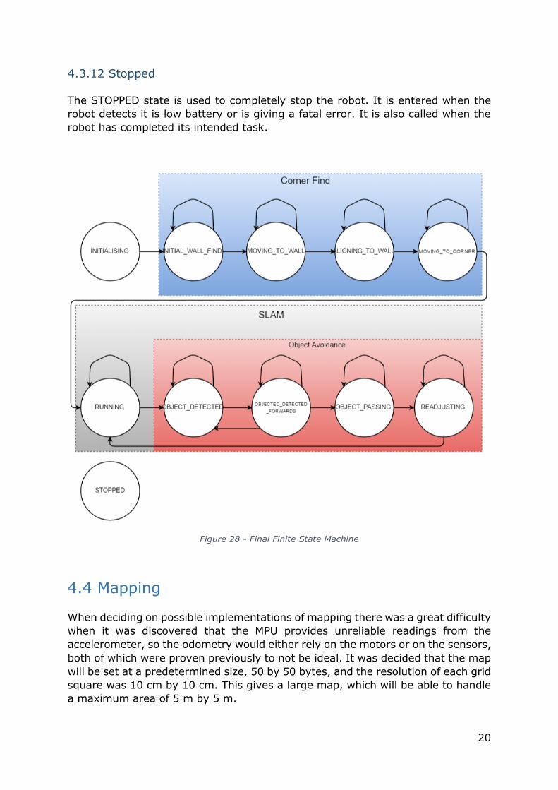
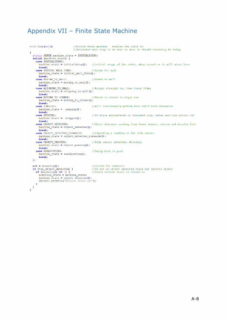
4.3 Finite State Machine
To realise the robot’s movements, a finite state machine was created that covers
each part of the movement, with a basic model shown in Figure 20. It begins at
initialising, finds the initial corner to use, runs through the inward spiral and avoids
Figure 20 - Basic Finite State Machine
15
obstacles, and ends with a stopped state. Every time a state loops, or another
state is called, the sensor outputs are read. If an object is detected the previous
state is noted, and object detection is executed. This allows obstacle detection to
be the highest priority state. The final Finite State Machine is shown at the end of
the section in Figure 28, and the code for the switching and the object detected
interrupt is shown in Appendix VII.
4.3.1 Initialisation
The initialisation sequence of the robot is primarily for setup. This is when the
robot can enable its motors, and test the sensors and MPU to ensure valid values
are being returned. It then passes to INITIAL_WALL_FIND.
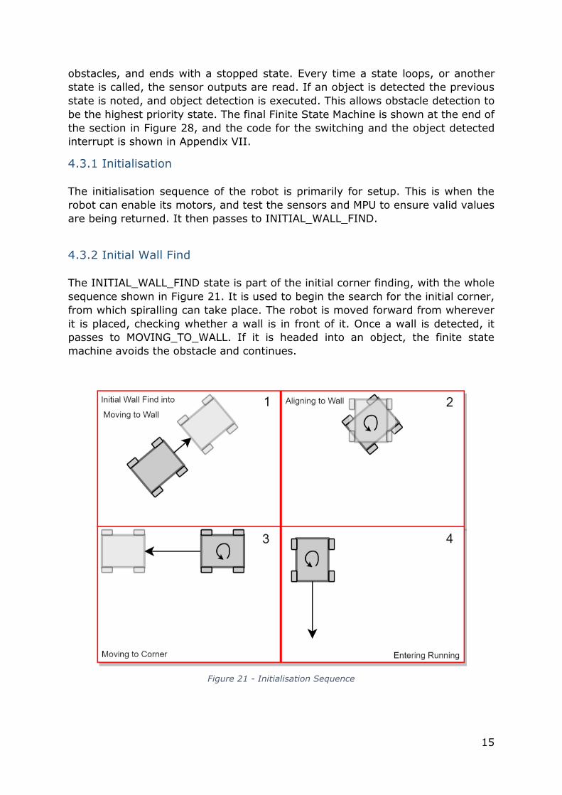
4.3.2 Initial Wall Find
The INITIAL_WALL_FIND state is part of the initial corner finding, with the whole
sequence shown in Figure 21. It is used to begin the search for the initial corner,
from which spiralling can take place. The robot is moved forward from wherever
it is placed, checking whether a wall is in front of it. Once a wall is detected, it
passes to MOVING_TO_WALL. If it is headed into an object, the finite state
machine avoids the obstacle and continues.
Figure 21 - Initialisation Sequence
16
4.3.3 Moving to Wall
The MOVING_TO_WALL state allows the robot to approach the wall slowly. The
robot moves forwards while all the forward facing sensors give a reading of more
than 30 cm. When under this distance, the robot’s movement decreases to 70%
of the speed. Once any of the front sensor readings are below a calibrated
distance, in this case being 18 cm, the robot stops and returns
ALIGNING_TO_WALL.
4.3.4 Aligning to Wall
In the ALIGNING_TO_WALL state the robot orients itself so that it is facing the
wall. This is done by comparing both of the forward-facing IR sensors and
determining which way the robot needs to rotate in order to face the wall. Once
the difference between the two sensors is below 3 cm the robot is determined to
be facing the wall. The robot then rotates counter-clockwise by 90° so that it will
be oriented parallel to the wall. Once this turn is complete the state changes to
MOVING_TO_CORNER.
4.3.5 Moving to Corner
The MOVING_TO_CORNER state moves the robot along the wall until it reaches
the first corner, which will begin the mapping sequence using the corner as a
definitive datum. When in this state, the robot will remains moving parallel to the
length of the wall until it reaches the corner, where it turns counter-clockwise by
90° and stop. If it begins to drift away or towards the wall, it realigns itself and
strafes back to the predetermined position using the align to wall function
discussed previously. Once the 90° turn is completed, the state is switched to
RUNNING.
4.3.6 Running
The RUNNING state keeps the robot moving in a spiral motion. The robot’s
movement is checked every 500 ms, and it realigns to be going parallel to the wall
every 750 ms. The time between consecutive align to wall calls represents a trade-
off between positional accuracy and speed, as the functionality available to move
the robot is limited to one degree of freedom at a single time. At 750 ms intervals
there was a suitable compromise where the robot would be able to move fast
enough while maintaining a sufficiently uniform distance away from the wall.
If the robot sees a wall ahead, it increments the corner count. Once the corner
count reaches three, it means that the next iteration will have to stop earlier, so
15 cm is added to the value the robot looks for in front of itself. Once the corner
count reaches four it means the spiral is complete, and the distance that it keeps
away from the walls on the side increases appropriately.
17
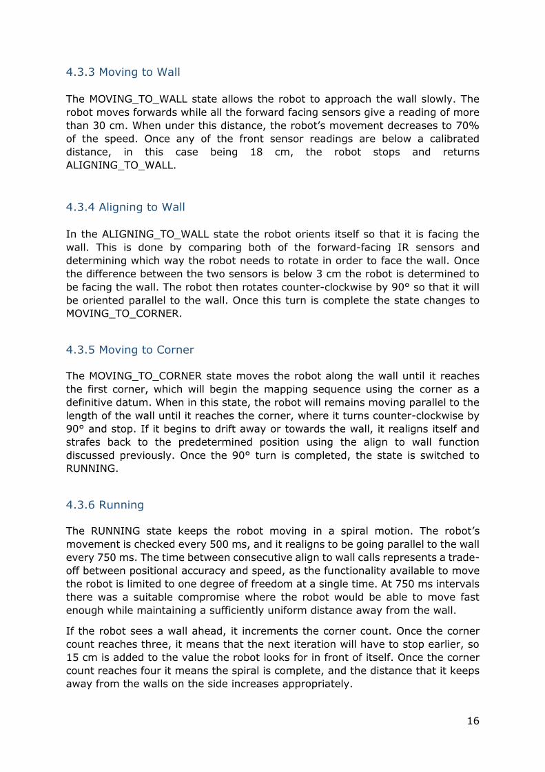
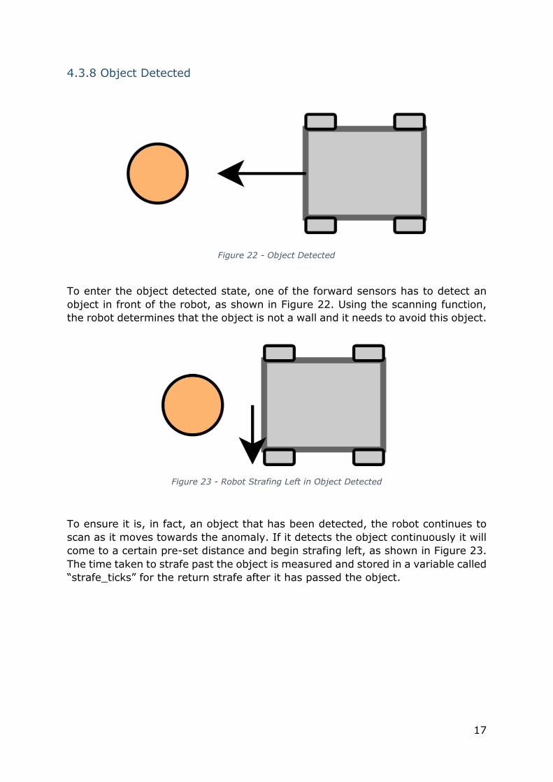
4.3.8 Object Detected
To enter the object detected state, one of the forward sensors has to detect an
object in front of the robot, as shown in Figure 22. Using the scanning function,
the robot determines that the object is not a wall and it needs to avoid this object.
To ensure it is, in fact, an object that has been detected, the robot continues to
scan as it moves towards the anomaly. If it detects the object continuously it will
come to a certain pre-set distance and begin strafing left, as shown in Figure 23.
The time taken to strafe past the object is measured and stored in a variable called
“strafe_ticks” for the return strafe after it has passed the object.
Figure 22 - Object Detected
Figure 23 - Robot Strafing Left in Object Detected
18
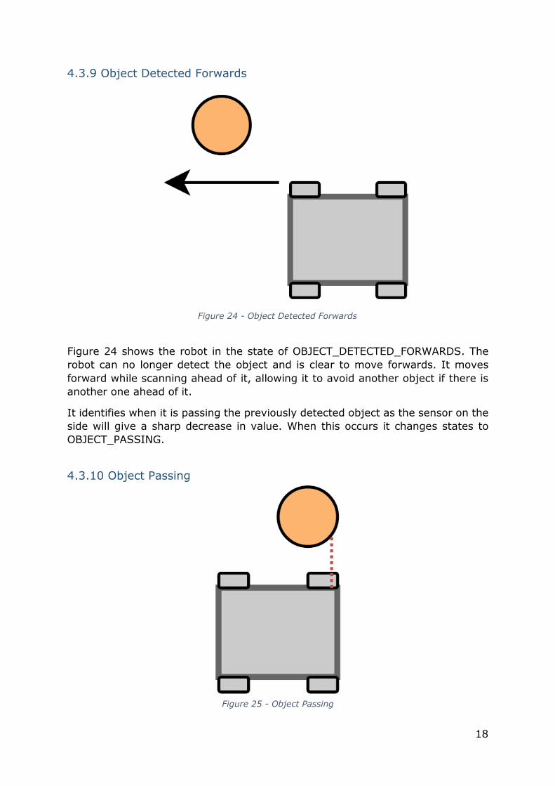
4.3.9 Object Detected Forwards
Figure 24 shows the robot in the state of OBJECT_DETECTED_FORWARDS. The
robot can no longer detect the object and is clear to move forwards. It moves
forward while scanning ahead of it, allowing it to avoid another object if there is
another one ahead of it.
It identifies when it is passing the previously detected object as the sensor on the
side will give a sharp decrease in value. When this occurs it changes states to
OBJECT_PASSING.
4.3.10 Object Passing
Figure 24 - Object Detected Forwards
Figure 25 - Object Passing
19
Object Passing, displayed in Figure 25, is a short state in which the rear side
sensor can detect the object as it passes it. When the robot has passed the object,
the sensor will no longer be outputting a short value and change into the state
READJUSTING.
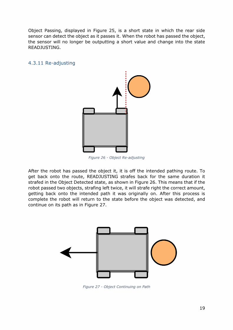
4.3.11 Re-adjusting
After the robot has passed the object it, it is off the intended pathing route. To
get back onto the route, READJUSTING strafes back for the same duration it
strafed in the Object Detected state, as shown in Figure 26. This means that if the
robot passed two objects, strafing left twice, it will strafe right the correct amount,
getting back onto the intended path it was originally on. After this process is
complete the robot will return to the state before the object was detected, and
continue on its path as in Figure 27.
Figure 26 - Object Re-adjusting
Figure 27 - Object Continuing on Path
20
4.3.12 Stopped
The STOPPED state is used to completely stop the robot. It is entered when the
robot detects it is low battery or is giving a fatal error. It is also called when the
robot has completed its intended task.
Figure 28 - Final Finite State Machine
4.4 Mapping
When deciding on possible implementations of mapping there was a great difficulty
when it was discovered that the MPU provides unreliable readings from the
accelerometer, so the odometry would either rely on the motors or on the sensors,
both of which were proven previously to not be ideal. It was decided that the map
will be set at a predetermined size, 50 by 50 bytes, and the resolution of each grid
square was 10 cm by 10 cm. This gives a large map, which will be able to handle
a maximum area of 5 m by 5 m.
21
A difficulty arose when trying to implement simple sensor odometry relying on the
front facing sensors. This idea was to use the original sensor reading at the start
of each length, relying mostly on the sonar. By subtracting the current sensor
readings, this would give the current position. The side sensors would give the
other coordinate. The problem arising was if an obstacle was in the current length
the front coordinate would be off, and hence the map would be plotted wrong.
The second method is relying on the wheels for odometry. The velocity for going
forward and strafing was measured, as well as the variations when lower speeds
were used for difficult manoeuvres. At the beginning of each length and
manoeuvre, a timer began, which when multiplied by the velocity output the
distance travelled. This was complemented with sensor readings for side
measurements. This method worked, however, the velocities varied greatly
depending on battery level. The robot was also found to not always be travelling
parallel to the wall as intended, which threw off the measurements.
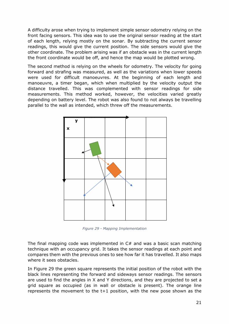
The final mapping code was implemented in C# and was a basic scan matching
technique with an occupancy grid. It takes the sensor readings at each point and
compares them with the previous ones to see how far it has travelled. It also maps
where it sees obstacles.
In Figure 29 the green square represents the initial position of the robot with the
black lines representing the forward and sideways sensor readings. The sensors
are used to find the angles in X and Y directions, and they are projected to set a
grid square as occupied (as in wall or obstacle is present). The orange line
represents the movement to the t+1 position, with the new pose shown as the
Figure 29 - Mapping Implementation
22
orange rectangle. This pose also sets the obstacle grids. By comparing the current
and previous pose’s sensor readings, the correct movement is logged and the pose
is charted on the grid. The pre-move x and y coordinates are added to the
movement values, and then divided by 10 to put in the correct square.
A difficulty was discovered with interfacing the Bluetooth with C#. Despite
troubleshooting this was not fixed in time for the assessment. However, this code
worked with example values within the debugger.
23
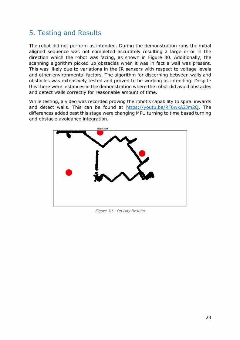
5. Testing and Results
The robot did not perform as intended. During the demonstration runs the initial
aligned sequence was not completed accurately resulting a large error in the
direction which the robot was facing, as shown in Figure 30. Additionally, the
scanning algorithm picked up obstacles when it was in fact a wall was present.
This was likely due to variations in the IR sensors with respect to voltage levels
and other environmental factors. The algorithm for discerning between walls and
obstacles was extensively tested and proved to be working as intending. Despite
this there were instances in the demonstration where the robot did avoid obstacles
and detect walls correctly for reasonable amount of time.
While testing, a video was recorded proving the robot’s capability to spiral inwards
and detect walls. This can be found at https://youtu.be/RF0wkA2Jm2Q. The
differences added past this stage were changing MPU turning to time based turning
and obstacle avoidance integration.
Figure 30 - On Day Results
24
6. Discussion, Limitations and Improvements
6.1 IR Sensors
The infrared sensors had multiple problems throughout the project. The range of
the sensors was about half of the range specified on the data sheet. Additionally,
some of the sensors would have a large variation in their output as the battery of
the robot was drained. Over a day of testing the calibration set at the start of the
day would become increasingly meaningless. Not knowing this at the start of the
project was the cause of significant delays to the continuation of it.
6.2 Number of Sensors
If the project allowed more sensors, this would allow better position control and
more freedom of movement. The limited number of sensors resulted in a large
blind spot where an object or a wall could not be detected. Any objects behind or
to the left of the robot could not be seen.
6.3 Motors The motors, although similar, did not have the same performance at each speed
level. The back left motor would run slower than the rest of the motors. The slower
speed was accounted for by running that motor faster than the others. This
approximation was useful however, it did not fully account for all the error.
Ultimately the motors worked well enough over the small distance specified in this
project, but over longer distances it would be advantageous to implement a control
system and state machine to continuously adjust for the different motor
characteristics.
6.4 Limited Movement Directions The use of simple movement functions which simplified the movement to one
direction or rotation at a time was helpful during the initial stages of development.
As the project progressed and a more accurate movements were desired it became
apparent the full functionality was not being used. A good example of this was the
aligning to wall function. A more sophisticated implementation would be to
individually control each wheel to move the robot back into the correct alignment
with the wall. Instead the robot would stop, strafe and then rotate to align to the
wall. This takes significantly more time to complete than a more sophisticated
approach. The simplifications did however allow for better odometry. As the robot
would only be moving in exactly one direction the distance moved would be
directly proportional to the time taken. This relationship proved to be useful in the
obstacle avoidance states and helped to offset the changes in motor speed with
respect to battery voltage.
25
6.5 Servo Motor Usage
This project allowed the use of a servo motor for mounting a sensor of the group’s
choosing to be free to rotate as programmed. This was not an option that was
taken, as it was felt that all the required sides were covered. However, in
hindsight, it would have been beneficial to utilise the servo motor, as it would
provide angle measurement capabilities, and the use of one sensor for more
directions, aiding with the limitations of the sensor placement. It would also check
corners for obstructions, as it was found due to sensor placement if the robot was
approaching the wall at too steep of an angle, the sensors could not identify the
obstacle.
6.6 MPU for Turning
The MPU was originally used for completing 90 degree turns, but was taken out
due to the slow response of the MPU causing constant overshooting in the turns.
This was replaced with a timed implementation of the turn. Although, initially tests
were positive, due to the varying speeds of the motors depending on battery level,
this quickly became troublesome. Unfortunately, due to time constraints, this
wasn’t fixed in time for the demonstration, and the presentation suffered greatly.
Ideally, the MPU should have been used for turning with input from the sensors
and some sort of closed loop control for achieving the perfect 90 degree turn.
6.7 PID Control
A PID controller would have theoretically resulted in no error when turning to face
and align to walls. However, the sensor data and the calibration used was not
accurate enough for this to be the case. A bang-bang or hysteresis controller was
chosen over a PID controller because it would be similarly accurate and
significantly quicker.
6.8 Fuzzy Logic In writing code such as that for aligning to wall, envelopes were developed, within
which range readings from the sensors were deemed acceptable for the robot to
be in. This would have been much better implemented through fuzzy logic. This
would have been done through defining distance and angle in relation to wall sets.
The output sets would include strafing away or towards the wall, and the steering
angle to correct the movement. This would have allowed a much smoother
alignment, without considerable overshoot which occurred.
26
6.9 Active SLAM This solution used entirely passive SLAM. Mapping was not considered in the path
planning algorithms and overall code functionality. If the mapping capabilities
were completed earlier, the map could have been used to feed information back
into the path planner, and create a better algorithm. This would not limit the
processing power significantly, but would provide a superior path for area
coverage and time required.
6.10 Finite State Machine
The implemented finite state machine was simplified significantly. The obstacle
avoidance states were implemented poorly not allowing the obstacle avoidance
sequence to be broken out of back to the running state unless the obstacle had
been completely avoided. In the demonstration this proved to be a large issue
especially in the rare case when a wall was mistakenly classified as an obstacle.
The number and function of each individual state was not mapped out from the
beginning of the project. A more complete planning process would have likely
resolved a lot of the state switching problems that were encountered.
7. Conclusion The autonomous SLAM robot project provided a great learning opportunity. It
allowed for the integration of hardware, electronics and software. The robot used
a finite state machine for operation, with an inward spiral path, strafing for object
avoidance and an occupancy grid for mapping. Despite the robot not functioning
as intended in the final presentation, it had a lot of potential for functionality, and
with further development and more time, would have been very successful in its
operation.
A-1
Appendices
Appendix I – Sonar Mount Drawing
Appendix II – MPU Mount Drawing
Appendix III – Ninety Turn Code
Appendix IV – Scanning Code
Appendix V – Get Sensor Data Code
Appendix VI – Align to Wall Code
Appendix VII – Finite State Machine
A-2
Appendix I – Sonar Mount Drawing
A-3
Appendix II – MPU Mount Drawing
A-4
Appendix III – Ninety Turn Code
A-5
Appendix IV – Scanning Code
A-6
Appendix V – Get Sensor Data Code
A-7
Appendix VI – Align to Wall Code
A-8
Appendix VII – Finite State Machine