THE JOURNAL OF CHEMICAL PHYSICS 135, 104115 (2011)

Mechanisms of kinetic trapping in self-assembly and phase transformationMichael F. Hagan,1 Oren M. Elrad,1 and Robert L. Jack2,a)

1Department of Physics, Brandeis University, Waltham, Massachusetts 02254, USA2Department of Physics, University of Bath, Bath BA2 7AY, United Kingdom

(Received 6 May 2011; accepted 18 August 2011; published online 14 September 2011)

In self-assembly processes, kinetic trapping effects often hinder the formation of thermodynamicallystable ordered states. In a model of viral capsid assembly and in the phase transformation of a latticegas, we show how simulations in a self-assembling steady state can be used to identify two distinctmechanisms of kinetic trapping. We argue that one of these mechanisms can be adequately capturedby kinetic rate equations, while the other involves a breakdown of theories that rely on cluster size asa reaction coordinate. We discuss how these observations might be useful in designing and optimisingself-assembly reactions. © 2011 American Institute of Physics. [doi:10.1063/1.3635775]

I. INTRODUCTION

In self-assembly processes, simple components come to-gether spontaneously to form ordered products. Such pro-cesses abound in biology, where the ordered structures mightbe the outer shells of viruses,1–5 extended one-dimensionalfilaments that make up the cytoskeleton,6 or ordered arraysof proteins on the surface of bacteria.7 In other areas ofnanoscience, self-assembled nanostructures made from cus-tomised DNA oligomers are being used to build ever morecomplex structures,8 and the possibility of tailoring interac-tions between colloidal particles to assemble diverse orderedstructures and phases is also an area of active research.9

Here, we concentrate on self-assembly processes that oc-cur without energy input. That is, we consider systems of in-teracting components, relaxing towards ordered equilibriumstates. In order to assemble a particular ordered structure,there are two requirements that must be met. Firstly, inter-actions between particles must be chosen so that the orderedstate minimises the system’s free energy and is, therefore, sta-ble at equilibrium. Secondly, one must address dynamic ques-tions: how long does it take for a system to reach its orderedequilibrium state, and how can interparticle interactions beoptimised to facilitate rapid and effective assembly?

Even if the equilibrium state of a system is ordered, thereare many scenarios in which formation of the relevant or-der occurs extremely slowly. In self-assembly, this is knownas “kinetic trapping.” In recent years, several studies4, 5, 10–18

have observed that self-assembly is most efficient when struc-tures are stabilised by large numbers of relatively weak in-teractions. In particular, while strong interparticle bonds sta-bilise the ordered equilibrium state, they are also associatedwith kinetic trapping effects that frustrate the assembly pro-cess. Instead, effective self-assembly proceeds by relativelytransient bond formation, including frequent bond-breakingevents.

Long ago, Caspar and Klug1 drew an analogy be-tween viral capsid assembly and phase changes such as

a)Author to whom correspondence should be addressed. Electronic mail:r.jack@bath.ac.uk.

crystallisation. Indeed, strong bonds may act to frustratecrystallisation dynamics and other phase change processes,just as they do in self-assembly. For example, phase trans-formations may be unobservable due to the formation ofamorphous aggregates,19 or to gelation.20 These are alsotypes of kinetic trapping, in that these systems are pre-vented from equilibrating into their ordered free-energyminima.

Our aim in this article is to consider mechanisms for ki-netic trapping that are generic, in that they apply across a largerange of systems. To this end, we consider two processes thatare apparently quite different: self-assembly of model viralcapsids and phase separation in the two-dimensional Ising lat-tice gas. Viral capsids are monodisperse closed shells madeof many identical smaller particles,1 while the ordered struc-tures that form in the lattice gas model are extended two-dimensional clusters. Yet, despite these differences betweentheir assembled products, we find that these models exhibitsome striking similarities and common features—we inter-pret these similarities as evidence for generic mechanismsby which dynamical effects frustrate the formation of orderedstates. Both crystallisation and capsid formation involve parti-cles undergoing rearrangement toward an ordered free energyminimum, so we use “self-assembly” as a broad term whichcovers both these processes.

In contrast to the studies of kinetic trapping basedon energy landscapes21–23 or schematic models of particleaggregation,19, 24 we do not attempt a detailed analysis of thestructures of the disordered states that lead to kinetic trap-ping in our model systems: at that level, the capsid and latticegas models are very different. Rather, our aims are firstly toidentify common features at the level of the assembly dynam-ics, and secondly to understand how the presence of kinetictraps may act to frustrate self-assembly and phase change, in-dependent of the structural features of the disordered states.In particular, we identify two generic trapping mechanisms,one of which can be captured by “classical” theories of phasechange,25, 26 while the other is associated with a breakdown ofthese theories. We discuss how deviations from the classicaltheory might be identified and characterised, based on ideasproposed by some of us.5

0021-9606/2011/135(10)/104115/13/$30.00 © 2011 American Institute of Physics135, 104115-1

Downloaded 15 Sep 2011 to 129.64.202.237. Redistribution subject to AIP license or copyright; see http://jcp.aip.org/about/rights_and_permissions

104115-2 Hagan, Elrad, and Jack J. Chem. Phys. 135, 104115 (2011)

II. MODELS

A. Viral capsid model

We first describe a model for the self-assembly of emptyicosahedral viral capsids. The model represents capsid pro-teins as rigid bodies (“subunits”) with excluded volume ge-ometries and orientation-dependent interactions. The lowestenergy structure is an icosahedral shell consisting of 20 sub-units (details are given in Appendix A and Fig. 8 as well asin Ref. 27). This model was used to examine the assembly oficosahedral viruses around a polymer in Ref. 27 and is simi-lar to models used by Rapaport et al.12, 28 and Nguyen et al.15

in simulations of empty capsid assembly. Each subunit couldcorrespond to a “capsomer” comprising a trimer of proteinsthat form a T = 1 capsid.

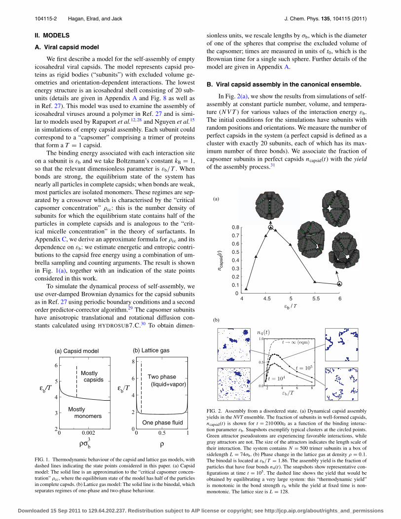
The binding energy associated with each interaction siteon a subunit is εb and we take Boltzmann’s constant kB = 1,so that the relevant dimensionless parameter is εb/T . Whenbonds are strong, the equilibrium state of the system hasnearly all particles in complete capsids; when bonds are weak,most particles are isolated monomers. These regimes are sep-arated by a crossover which is characterised by the “criticalcapsomer concentration” ρcc: this is the number density ofsubunits for which the equilibrium state contains half of theparticles in complete capsids and is analogous to the “crit-ical micelle concentration” in the theory of surfactants. InAppendix C, we derive an approximate formula for ρcc and itsdependence on εb: we estimate energetic and entropic contri-butions to the capsid free energy using a combination of um-brella sampling and counting arguments. The result is shownin Fig. 1(a), together with an indication of the state pointsconsidered in this work.

To simulate the dynamical process of self-assembly, weuse over-damped Brownian dynamics for the capsid subunitsas in Ref. 27 using periodic boundary conditions and a secondorder predictor-corrector algorithm.29 The capsomer subunitshave anisotropic translational and rotational diffusion con-stants calculated using HYDROSUB7.C.30 To obtain dimen-

0 0.002

ρσb

3

2

3

4

5

6

εb/T

0 0.5 1

ρ

0

2

4

6

8

εb/T

One phase fluid

Two phase(liquid+vapor)

Mostly

Mostlymonomers

capsids

(b) Lattice gas(a) Capsid model

FIG. 1. Thermodynamic behaviour of the capsid and lattice gas models, withdashed lines indicating the state points considered in this paper. (a) Capsidmodel: The solid line is an approximation to the “critical capsomer concen-tration” ρcc, where the equilibrium state of the model has half of the particlesin complete capsds. (b) Lattice gas model: The solid line is the binodal, whichseparates regimes of one-phase and two-phase behaviour.

sionless units, we rescale lengths by σb, which is the diameterof one of the spheres that comprise the excluded volume ofthe capsomer; times are measured in units of t0, which is theBrownian time for a single such sphere. Further details of themodel are given in Appendix A.

B. Viral capsid assembly in the canonical ensemble.

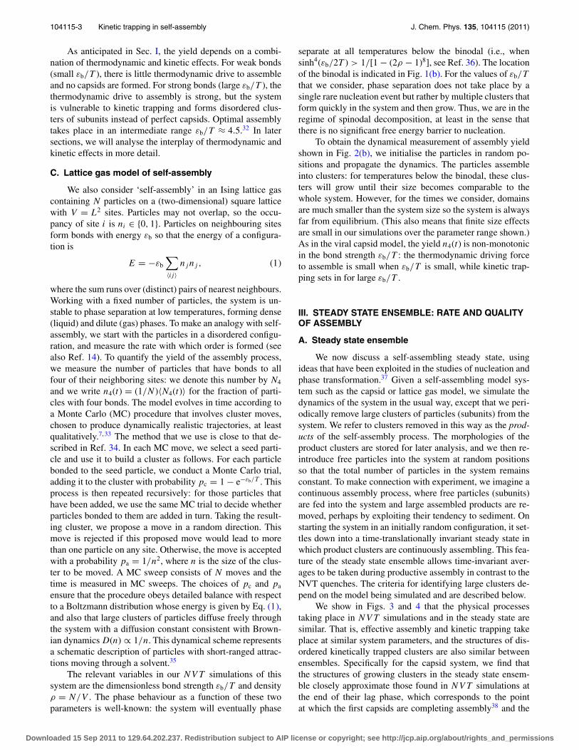
In Fig. 2(a), we show the results from simulations of self-assembly at constant particle number, volume, and tempera-ture (NV T ) for various values of the interaction energy εb.The initial conditions for the simulations have subunits withrandom positions and orientations. We measure the number ofperfect capsids in the system (a perfect capsid is defined as acluster with exactly 20 subunits, each of which has its max-imum number of three bonds). We associate the fraction ofcapsomer subunits in perfect capsids ncapsid(t) with the yieldof the assembly process.31

0

0.1

0.2

0.3

0.4

0.5

0.6

0.7

0.8

4 4.5 5 5.5 6

caps

id(t

)

b / T

εb/T

n4(t)

t = 105

t = 104

t → ∞ (eqm)

(a)

(b)

FIG. 2. Assembly from a disordered state. (a) Dynamical capsid assemblyyields in the NVT ensemble. The fraction of subunits in well-formed capsids,ncapsid(t) is shown for t = 210 000t0 as a function of the binding interac-tion parameter εb. Snapshots exemplify typical clusters at the circled points.Green attractor pseudoatoms are experiencing favorable interactions, whilegray attractors are not. The size of the attractors indicates the length scale oftheir interaction. The system contains N = 500 trimer subunits in a box ofsidelength L = 74σb. (b) Phase change in the lattice gas at density ρ = 0.1.The binodal is located at εb/T = 1.86. The assembly yield is the fraction ofparticles that have four bonds n4(t). The snapshots show representative con-figurations at time t = 105. The dashed line shows the yield that would beobtained by equilibrating a very large system: this “thermodynamic yield”is monotonic in the bond strength εb while the yield at fixed time is non-monotonic. The lattice size is L = 128.

Downloaded 15 Sep 2011 to 129.64.202.237. Redistribution subject to AIP license or copyright; see http://jcp.aip.org/about/rights_and_permissions

104115-3 Kinetic trapping in self-assembly J. Chem. Phys. 135, 104115 (2011)

As anticipated in Sec. I, the yield depends on a combi-nation of thermodynamic and kinetic effects. For weak bonds(small εb/T ), there is little thermodynamic drive to assembleand no capsids are formed. For strong bonds (large εb/T ), thethermodynamic drive to assembly is strong, but the systemis vulnerable to kinetic trapping and forms disordered clus-ters of subunits instead of perfect capsids. Optimal assemblytakes place in an intermediate range εb/T ≈ 4.5.32 In latersections, we will analyse the interplay of thermodynamic andkinetic effects in more detail.

C. Lattice gas model of self-assembly

We also consider ‘self-assembly’ in an Ising lattice gascontaining N particles on a (two-dimensional) square latticewith V = L2 sites. Particles may not overlap, so the occu-pancy of site i is ni ∈ {0, 1}. Particles on neighbouring sitesform bonds with energy εb so that the energy of a configura-tion is

E = −εb

∑〈ij〉

njnj , (1)

where the sum runs over (distinct) pairs of nearest neighbours.Working with a fixed number of particles, the system is un-stable to phase separation at low temperatures, forming dense(liquid) and dilute (gas) phases. To make an analogy with self-assembly, we start with the particles in a disordered configu-ration, and measure the rate with which order is formed (seealso Ref. 14). To quantify the yield of the assembly process,we measure the number of particles that have bonds to allfour of their neighboring sites: we denote this number by N4

and we write n4(t) = (1/N )〈N4(t)〉 for the fraction of parti-cles with four bonds. The model evolves in time according toa Monte Carlo (MC) procedure that involves cluster moves,chosen to produce dynamically realistic trajectories, at leastqualitatively.7, 33 The method that we use is close to that de-scribed in Ref. 34. In each MC move, we select a seed parti-cle and use it to build a cluster as follows. For each particlebonded to the seed particle, we conduct a Monte Carlo trial,adding it to the cluster with probability pc = 1 − e−εb/T . Thisprocess is then repeated recursively: for those particles thathave been added, we use the same MC trial to decide whetherparticles bonded to them are added in turn. Taking the result-ing cluster, we propose a move in a random direction. Thismove is rejected if this proposed move would lead to morethan one particle on any site. Otherwise, the move is acceptedwith a probability pa = 1/n2, where n is the size of the clus-ter to be moved. A MC sweep consists of N moves and thetime is measured in MC sweeps. The choices of pc and pa

ensure that the procedure obeys detailed balance with respectto a Boltzmann distribution whose energy is given by Eq. (1),and also that large clusters of particles diffuse freely throughthe system with a diffusion constant consistent with Brown-ian dynamics D(n) ∝ 1/n. This dynamical scheme representsa schematic description of particles with short-ranged attrac-tions moving through a solvent.35

The relevant variables in our NV T simulations of thissystem are the dimensionless bond strength εb/T and densityρ = N/V . The phase behaviour as a function of these twoparameters is well-known: the system will eventually phase

separate at all temperatures below the binodal (i.e., whensinh4(εb/2T ) > 1/[1 − (2ρ − 1)8], see Ref. 36). The locationof the binodal is indicated in Fig. 1(b). For the values of εb/T

that we consider, phase separation does not take place by asingle rare nucleation event but rather by multiple clusters thatform quickly in the system and then grow. Thus, we are in theregime of spinodal decomposition, at least in the sense thatthere is no significant free energy barrier to nucleation.

To obtain the dynamical measurement of assembly yieldshown in Fig. 2(b), we initialise the particles in random po-sitions and propagate the dynamics. The particles assembleinto clusters: for temperatures below the binodal, these clus-ters will grow until their size becomes comparable to thewhole system. However, for the times we consider, domainsare much smaller than the system size so the system is alwaysfar from equilibrium. (This also means that finite size effectsare small in our simulations over the parameter range shown.)As in the viral capsid model, the yield n4(t) is non-monotonicin the bond strength εb/T : the thermodynamic driving forceto assemble is small when εb/T is small, while kinetic trap-ping sets in for large εb/T .

III. STEADY STATE ENSEMBLE: RATE AND QUALITYOF ASSEMBLY

A. Steady state ensemble

We now discuss a self-assembling steady state, usingideas that have been exploited in the studies of nucleation andphase transformation.37 Given a self-assembling model sys-tem such as the capsid or lattice gas model, we simulate thedynamics of the system in the usual way, except that we peri-odically remove large clusters of particles (subunits) from thesystem. We refer to clusters removed in this way as the prod-ucts of the self-assembly process. The morphologies of theproduct clusters are stored for later analysis, and we then re-introduce free particles into the system at random positionsso that the total number of particles in the system remainsconstant. To make connection with experiment, we imagine acontinuous assembly process, where free particles (subunits)are fed into the system and large assembled products are re-moved, perhaps by exploiting their tendency to sediment. Onstarting the system in an initially random configuration, it set-tles down into a time-translationally invariant steady state inwhich product clusters are continuously assembling. This fea-ture of the steady state ensemble allows time-invariant aver-ages to be taken during productive assembly in contrast to theNVT quenches. The criteria for identifying large clusters de-pend on the model being simulated and are described below.

We show in Figs. 3 and 4 that the physical processestaking place in NV T simulations and in the steady state aresimilar. That is, effective assembly and kinetic trapping takeplace at similar system parameters, and the structures of dis-ordered kinetically trapped clusters are also similar betweenensembles. Specifically for the capsid system, we find thatthe structures of growing clusters in the steady state ensem-ble closely approximate those found in NV T simulations atthe end of their lag phase, which corresponds to the pointat which the first capsids are completing assembly38 and the

Downloaded 15 Sep 2011 to 129.64.202.237. Redistribution subject to AIP license or copyright; see http://jcp.aip.org/about/rights_and_permissions

104115-4 Hagan, Elrad, and Jack J. Chem. Phys. 135, 104115 (2011)

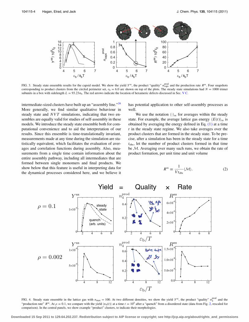
FIG. 3. Steady state ensemble results for the capsid model. We show the yield Y ss, the product “quality” nprodcaps and the production rate Rss. Four snapshots

corresponding to product clusters from the circled perimeter set, εb = 6.0 are shown on top of the plots. The steady state simulations had N = 1000 trimersubunits in a box with sidelength L = 93.23σb. The red arrows indicate the location of hexameric defects discussed in Sec. V C.

intermediate-sized clusters have built up an “assembly line.”39

More generally, we find similar qualitative behaviour insteady state and NV T simulations, indicating that two en-sembles are equally valid for studies of self-assembly in thesemodels. We introduce the steady state ensemble both for com-putational convenience and to aid the interpretation of ourresults. Since this ensemble is time-translationally invariant,measurements made at any time during the simulation are sta-tistically equivalent, which facilitates the evaluation of aver-ages and correlation functions during assembly. Also, mea-surements from a single time contain information about theentire assembly pathway, including all intermediates that areformed between single monomers and final products. Weshow below that this feature is useful in interpreting data forthe dynamical processes considered here, and we believe it

has potential application to other self-assembly processes aswell.

We use the notation 〈·〉ss for averages within the steadystate. For example, the average lattice gas energy 〈E(t)〉ss isobtained by averaging the energy defined in Eq. (1) at a timet in the steady state regime. We also take averages over theproduct clusters that are formed in the steady state. To be pre-cise, after a simulation has been in the steady state for a timetobs, let the number of product clusters formed in that timebe M. Averaging over many such runs, we obtain the rate ofproduct formation, per unit time and unit volume

Rss ≡ 1

V tobs〈M〉. (2)

4 8 120

5 10-9

1 10-8

4 8 120

0.2

0.4

0.6

4 8 120.0

5.0 10-9

1.0 10-8

1.5 10-8

2 4 6 80

1 10-6

2 4 6 80

0.2

0.4

2 4 6 80

2 10-6

4 10-6

6 10-6

εb/T

Yield Quality Rate=Y ss nprod

4 Rss

ρ = 0.1 steady state

quench (arb. units)

εb/T

ρ = 0.002

Y ss nprod4 Rss

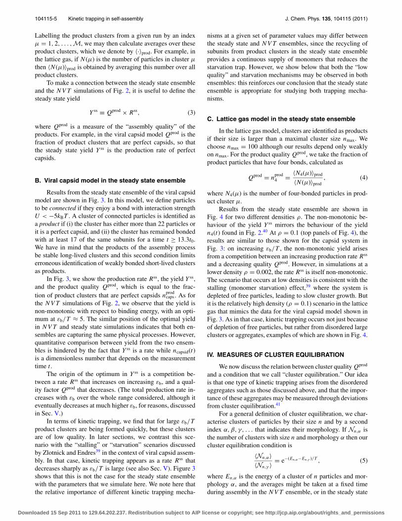
FIG. 4. Steady state ensemble in the lattice gas with nmax = 100. At two different densities, we show the yield Y ss, the product “quality” nprod4 and the

“production rate” Rss. At ρ = 0.1, we compare with the yield 〈n4(t)〉 at a time t = 105 after a “quench” from a disordered state (data from Fig. 2, rescaled forcomparison). In the central panels, we show example “product” clusters, to indicate their morphologies.

Downloaded 15 Sep 2011 to 129.64.202.237. Redistribution subject to AIP license or copyright; see http://jcp.aip.org/about/rights_and_permissions

104115-5 Kinetic trapping in self-assembly J. Chem. Phys. 135, 104115 (2011)

Labelling the product clusters from a given run by an indexμ = 1, 2, . . . ,M, we may then calculate averages over theseproduct clusters, which we denote by 〈·〉prod. For example, inthe lattice gas, if N (μ) is the number of particles in cluster μ

then 〈N (μ)〉prod is obtained by averaging this number over allproduct clusters.

To make a connection between the steady state ensembleand the NV T simulations of Fig. 2, it is useful to define thesteady state yield

Y ss ≡ Qprod × Rss, (3)

where Qprod is a measure of the “assembly quality” of theproducts. For example, in the viral capsid model Qprod is thefraction of product clusters that are perfect capsids, so thatthe steady state yield Y ss is the production rate of perfectcapsids.

B. Viral capsid model in the steady state ensemble

Results from the steady state ensemble of the viral capsidmodel are shown in Fig. 3. In this model, we define particlesto be connected if they enjoy a bond with interaction strengthU < −5kBT . A cluster of connected particles is identified asa product if (i) the cluster has either more than 22 particles orit is a perfect capsid, and (ii) the cluster has remained bondedwith at least 17 of the same subunits for a time t ≥ 13.3t0.We have in mind that the products of the assembly processbe stable long-lived clusters and this second condition limitserroneous identification of weakly bonded short-lived clustersas products.

In Fig. 3, we show the production rate Rss, the yield Y ss,and the product quality Qprod, which is equal to the frac-tion of product clusters that are perfect capsids n

prodcaps . As for

the NV T simulations of Fig. 2, we observe that the yield isnon-monotonic with respect to binding energy, with an opti-mum at εb/T ≈ 5. The similar position of the optimal yieldin NV T and steady state simulations indicates that both en-sembles are capturing the same physical processes. However,quantitative comparison between yield from the two ensem-bles is hindered by the fact that Y ss is a rate while ncapsid(t)is a dimensionless number that depends on the measurementtime t .

The origin of the optimum in Y ss is a competition be-tween a rate Rss that increases on increasing εb, and a qual-ity factor Qprod that decreases. (The total production rate in-creases with εb over the whole range considered, although iteventually decreases at much higher εb, for reasons, discussedin Sec. V.)

In terms of kinetic trapping, we find that for large εb/T

product clusters are being formed quickly, but these clustersare of low quality. In later sections, we contrast this sce-nario with the “stalling” or “starvation” scenarios discussedby Zlotnick and Endres39 in the context of viral capsid assem-bly. In that case, kinetic trapping appears as a rate Rss thatdecreases sharply as εb/T is large (see also Sec. V). Figure 3shows that this is not the case for the steady state ensemblewith the parameters that we simulate here. We note here thatthe relative importance of different kinetic trapping mecha-

nisms at a given set of parameter values may differ betweenthe steady state and NV T ensembles, since the recycling ofsubunits from product clusters in the steady state ensembleprovides a continuous supply of monomers that reduces thestarvation trap. However, we show below that both the “lowquality” and starvation mechanisms may be observed in bothensembles: this reinforces our conclusion that the steady stateensemble is appropriate for studying both trapping mecha-nisms.

C. Lattice gas model in the steady state ensemble

In the lattice gas model, clusters are identified as productsif their size is larger than a maximal cluster size nmax. Wechoose nmax = 100 although our results depend only weaklyon nmax. For the product quality Qprod, we take the fraction ofproduct particles that have four bonds, calculated as

Qprod = nprod4 = 〈N4(μ)〉prod

〈N (μ)〉prod, (4)

where N4(μ) is the number of four-bonded particles in prod-uct cluster μ.

Results from the steady state ensemble are shown inFig. 4 for two different densities ρ. The non-monotonic be-haviour of the yield Y ss mirrors the behaviour of the yieldn4(t) found in Fig. 2.40 At ρ = 0.1 (top panels of Fig. 4), theresults are similar to those shown for the capsid system inFig. 3: on increasing εb/T , the non-monotonic yield arisesfrom a competition between an increasing production rate Rss

and a decreasing quality Qprod. However, in simulations at alower density ρ = 0.002, the rate Rss is itself non-monotonic.The scenario that occurs at low densities is consistent with thestalling (monomer starvation) effect,39 where the system isdepleted of free particles, leading to slow cluster growth. Butit is the relatively high density (ρ = 0.1) scenario in the latticegas that mimics the data for the viral capsid model shown inFig. 3. As in that case, kinetic trapping occurs not just becauseof depletion of free particles, but rather from disordered largeclusters or aggregates, examples of which are shown in Fig. 4.

IV. MEASURES OF CLUSTER EQUILIBRATION

We now discuss the relation between cluster quality Qprod

and a condition that we call “cluster equilibration.” Our ideais that one type of kinetic trapping arises from the disorderedaggregates such as those discussed above, and that the impor-tance of these aggregates may be measured through deviationsfrom cluster equilibration.41

For a general definition of cluster equilibration, we char-acterise clusters of particles by their size n and by a secondindex α, β, γ, . . . that indicates their morphology. If Nn,α isthe number of clusters with size n and morphology α then ourcluster equilibration condition is

〈Nn,α〉〈Nn,γ 〉 = e−(En,α−En,γ )/T , (5)

where En,α is the energy of a cluster of n particles and mor-phology α, and the averages might be taken at a fixed timeduring assembly in the NV T ensemble, or in the steady state

Downloaded 15 Sep 2011 to 129.64.202.237. Redistribution subject to AIP license or copyright; see http://jcp.aip.org/about/rights_and_permissions

104115-6 Hagan, Elrad, and Jack J. Chem. Phys. 135, 104115 (2011)

ensemble. In words, Eq. (5) states that: “for clusters of sizen, the probabilities of different morphologies are Boltzmann-distributed.” It seems natural to interpret this as a clusterequilibration condition. (If the clusters have different ex-cluded volumes one might take this into account by replacingthe energy with a suitable enthalpy, and any internal entropyof the cluster can also be incorporated through a cluster freeenergy.) In theoretical treatments of self-assembly based onrate equations or field-theoretic arguments, it is natural to as-sume that Eq. (5) holds (see Sec. V). We now show that de-viations from Eq. (5) are significant throughout the regimeswhere kinetic trapping is important indicating that such devi-ations must be taken into account in theories of self-assembly.

A. Cluster equilibration in the lattice gas model

In the self-assembling steady state of the lattice gasmodel, we count the number of four-bonded particles withineach cluster. We average this quantity over clusters of a fixedsize n, and we denote this average by 〈N4(n)〉ss. We emphasisethat these are the averages over clusters in the self-assemblingsteady state, and not over the product clusters. It is conve-nient to compare 〈N4(n)〉ss with N

gs4 (n), which is the number

of four-bonded particles in a cluster of size n that minimisesthe cluster energy. We then define

〈�n4(n)〉ss = 1

n

⟨N4(n) − N

gs4 (n)

⟩ss (6)

to measure the deviation of the cluster “quality” from itsground state value, normalised by the cluster size n.

To test the extent of cluster equilibration, we have per-formed umbrella sampling, in which we choose a maximalcluster size numb and reject all MC moves that form clustersof size bigger than numb. On propagating the dynamics, thesystem relaxes to a state that satisfies this constraint but isotherwise equilibrated, so that we expect Eq. (5) to hold.42, 59

In the umbrella-sampled ensemble, we again measure thenumber of particles with four bonds and average over clus-ters of size n. The analogue of Eq. (6) within this ensem-ble is 〈�n4(n)〉umb = 1

n〈N4(n) − N

gs4 (n)〉umb. Comparison of

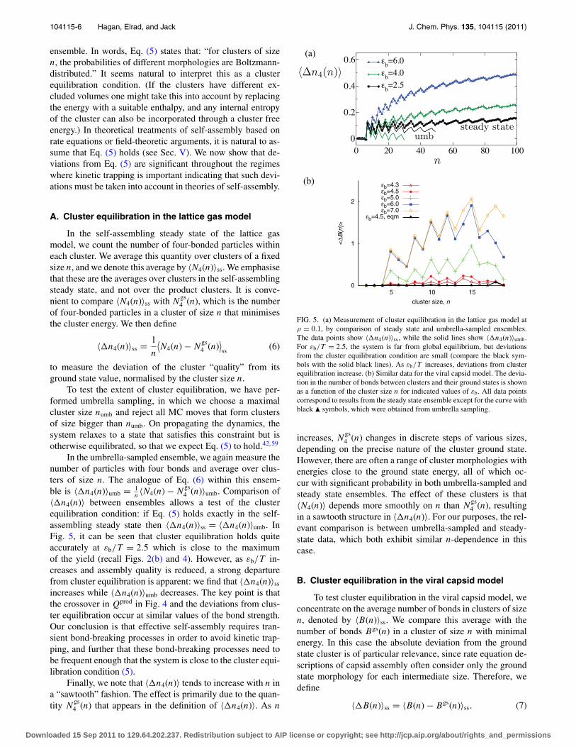
〈�n4(n)〉 between ensembles allows a test of the clusterequilibration condition: if Eq. (5) holds exactly in the self-assembling steady state then 〈�n4(n)〉ss = 〈�n4(n)〉umb. InFig. 5, it can be seen that cluster equilibration holds quiteaccurately at εb/T = 2.5 which is close to the maximumof the yield (recall Figs. 2(b) and 4). However, as εb/T in-creases and assembly quality is reduced, a strong departurefrom cluster equilibration is apparent: we find that 〈�n4(n)〉ss

increases while 〈�n4(n)〉umb decreases. The key point is thatthe crossover in Qprod in Fig. 4 and the deviations from clus-ter equilibration occur at similar values of the bond strength.Our conclusion is that effective self-assembly requires tran-sient bond-breaking processes in order to avoid kinetic trap-ping, and further that these bond-breaking processes need tobe frequent enough that the system is close to the cluster equi-libration condition (5).

Finally, we note that 〈�n4(n)〉 tends to increase with n ina “sawtooth” fashion. The effect is primarily due to the quan-tity N

gs4 (n) that appears in the definition of 〈�n4(n)〉. As n

Δn4(n)

n

umbsteady state

0

1

2

5 10 15

<ΔB

(n)>

cluster size, n

εb=4.3εb=4.5εb=5.0εb=6.0εb=7.0

εb=4.5, eqm

(b)

(a)

FIG. 5. (a) Measurement of cluster equilibration in the lattice gas model atρ = 0.1, by comparison of steady state and umbrella-sampled ensembles.The data points show 〈�n4(n)〉ss, while the solid lines show 〈�n4(n)〉umb.For εb/T = 2.5, the system is far from global equilibrium, but deviationsfrom the cluster equilibration condition are small (compare the black sym-bols with the solid black lines). As εb/T increases, deviations from clusterequilibration increase. (b) Similar data for the viral capsid model. The devia-tion in the number of bonds between clusters and their ground states is shownas a function of the cluster size n for indicated values of εb. All data pointscorrespond to results from the steady state ensemble except for the curve withblack � symbols, which were obtained from umbrella sampling.

increases, Ngs4 (n) changes in discrete steps of various sizes,

depending on the precise nature of the cluster ground state.However, there are often a range of cluster morphologies withenergies close to the ground state energy, all of which oc-cur with significant probability in both umbrella-sampled andsteady state ensembles. The effect of these clusters is that〈N4(n)〉 depends more smoothly on n than N

gs4 (n), resulting

in a sawtooth structure in 〈�n4(n)〉. For our purposes, the rel-evant comparison is between umbrella-sampled and steady-state data, which both exhibit similar n-dependence in thiscase.

B. Cluster equilibration in the viral capsid model

To test cluster equilibration in the viral capsid model, weconcentrate on the average number of bonds in clusters of sizen, denoted by 〈B(n)〉ss. We compare this average with thenumber of bonds Bgs(n) in a cluster of size n with minimalenergy. In this case the absolute deviation from the groundstate cluster is of particular relevance, since rate equation de-scriptions of capsid assembly often consider only the groundstate morphology for each intermediate size. Therefore, wedefine

〈�B(n)〉ss = 〈B(n) − Bgs(n)〉ss. (7)

Downloaded 15 Sep 2011 to 129.64.202.237. Redistribution subject to AIP license or copyright; see http://jcp.aip.org/about/rights_and_permissions

104115-7 Kinetic trapping in self-assembly J. Chem. Phys. 135, 104115 (2011)

Note that this deviation is not normalised by the cluster sizen. As for the lattice gas, we perform umbrella sampling thatprohibits the formation of clusters larger than numb. (Specif-ically, we use a hybrid Brownian dynamics/Monte Carlo ap-proach where we use a short sequence of unbiased Browniandynamics steps as a trial move, which is rejected if the size ofthe largest cluster is greater than numb.)

Results for 〈�B(n)〉 are shown in Fig. 5. For theumbrella-sampled data, we find that 〈�B(n)〉umb ≈ 0 for εb

= 4.5: this quantity is similarly small for εb > 4.5. (The ap-parent deviation from 〈�B(n)〉umb ≈ 0 at n = 18 in Fig. 5is likely a result of imperfect equilibration in the umbrella-sampled simulations.) As in the lattice gas data, the steadystate measurements show that deviations from cluster equili-bration are small near optimal assembly, and grow as kinetictrapping sets in and Qprod decreases.

As in the lattice gas, a sawtooth structure is visible in〈�B(n)〉ss. Here, increasing the cluster size n leads to achange of either one or two bonds in Bgs(n). As 〈�B(n)〉ss

deviates from Bgs(n), there are several relevant cluster mor-phologies in the steady state ensemble which average out thestep changes that occur in Bgs(n): typically, the change in〈B(n)〉ss on increasing n would be somewhere between 1 and2 bonds. The combination of discrete changes in Bgs(n) andsmoother changes in 〈B(n)〉ss results in the apparent sawtoothpattern.

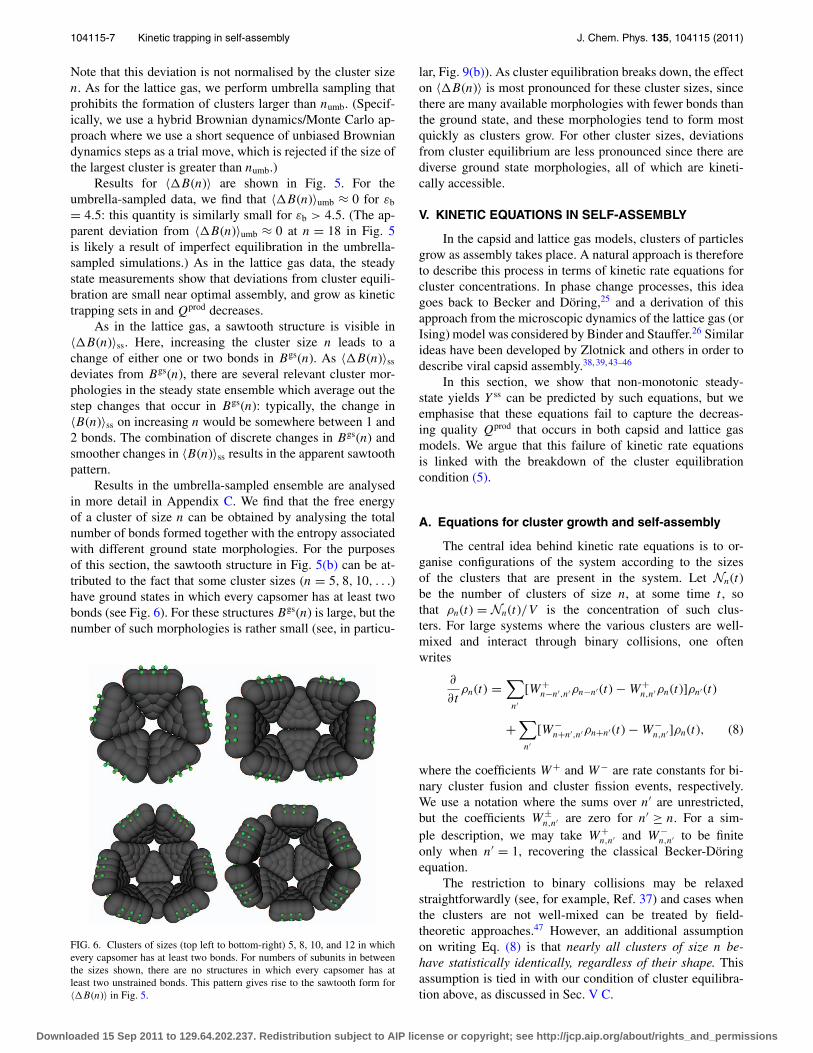
Results in the umbrella-sampled ensemble are analysedin more detail in Appendix C. We find that the free energyof a cluster of size n can be obtained by analysing the totalnumber of bonds formed together with the entropy associatedwith different ground state morphologies. For the purposesof this section, the sawtooth structure in Fig. 5(b) can be at-tributed to the fact that some cluster sizes (n = 5, 8, 10, . . .)have ground states in which every capsomer has at least twobonds (see Fig. 6). For these structures Bgs(n) is large, but thenumber of such morphologies is rather small (see, in particu-

FIG. 6. Clusters of sizes (top left to bottom-right) 5, 8, 10, and 12 in whichevery capsomer has at least two bonds. For numbers of subunits in betweenthe sizes shown, there are no structures in which every capsomer has atleast two unstrained bonds. This pattern gives rise to the sawtooth form for〈�B(n)〉 in Fig. 5.

lar, Fig. 9(b)). As cluster equilibration breaks down, the effecton 〈�B(n)〉 is most pronounced for these cluster sizes, sincethere are many available morphologies with fewer bonds thanthe ground state, and these morphologies tend to form mostquickly as clusters grow. For other cluster sizes, deviationsfrom cluster equilibrium are less pronounced since there arediverse ground state morphologies, all of which are kineti-cally accessible.

V. KINETIC EQUATIONS IN SELF-ASSEMBLY

In the capsid and lattice gas models, clusters of particlesgrow as assembly takes place. A natural approach is thereforeto describe this process in terms of kinetic rate equations forcluster concentrations. In phase change processes, this ideagoes back to Becker and Döring,25 and a derivation of thisapproach from the microscopic dynamics of the lattice gas (orIsing) model was considered by Binder and Stauffer.26 Similarideas have been developed by Zlotnick and others in order todescribe viral capsid assembly.38, 39, 43–46

In this section, we show that non-monotonic steady-state yields Y ss can be predicted by such equations, but weemphasise that these equations fail to capture the decreas-ing quality Qprod that occurs in both capsid and lattice gasmodels. We argue that this failure of kinetic rate equationsis linked with the breakdown of the cluster equilibrationcondition (5).

A. Equations for cluster growth and self-assembly

The central idea behind kinetic rate equations is to or-ganise configurations of the system according to the sizesof the clusters that are present in the system. Let Nn(t)be the number of clusters of size n, at some time t , sothat ρn(t) = Nn(t)/V is the concentration of such clus-ters. For large systems where the various clusters are well-mixed and interact through binary collisions, one oftenwrites

∂

∂tρn(t) =

∑n′

[W+n−n′,n′ρn−n′ (t) − W+

n,n′ρn(t)]ρn′(t)

+∑n′

[W−n+n′,n′ρn+n′ (t) − W−

n,n′ ]ρn(t), (8)

where the coefficients W+ and W− are rate constants for bi-nary cluster fusion and cluster fission events, respectively.We use a notation where the sums over n′ are unrestricted,but the coefficients W±

n,n′ are zero for n′ ≥ n. For a sim-ple description, we may take W+

n,n′ and W−n,n′ to be finite

only when n′ = 1, recovering the classical Becker-Döringequation.

The restriction to binary collisions may be relaxedstraightforwardly (see, for example, Ref. 37) and cases whenthe clusters are not well-mixed can be treated by field-theoretic approaches.47 However, an additional assumptionon writing Eq. (8) is that nearly all clusters of size n be-have statistically identically, regardless of their shape. Thisassumption is tied in with our condition of cluster equilibra-tion above, as discussed in Sec. V C.

Downloaded 15 Sep 2011 to 129.64.202.237. Redistribution subject to AIP license or copyright; see http://jcp.aip.org/about/rights_and_permissions

104115-8 Hagan, Elrad, and Jack J. Chem. Phys. 135, 104115 (2011)

B. Non-monotonic production rate R in kineticequations

The steady state ensemble has a natural realisation interms of these kinetic rate equations. To keep a compact no-tation, we write M = nmax − 1 as the size of the largest clus-ters that are not removed as products. We consider clusters ofsizes n = 1 . . . M , and we restrict ourselves for convenienceto monomer binding and unbinding. Then, for 1 < n < M wehave

∂

∂tρn(t) = Dρ1(t)[ρn−1(t) − ρn(t)] + λn+1ρn+1(t) − λnρn(t)

(9)For simplicity, we have replaced the n-dependent rateconstants by a single “diffusion-limited” rate D,48 and λn

is the rate for unbinding of a monomer from a cluster ofsize n. If the system is allowed to equilibrate, we have thatρ

eqn = ρ

eq1

∏nr=2(Dρ

eq1 /λr ). In comparing with lattice gas or

capsid models, we expect monomer binding and unbindingrates to be related by detailed balance, as

D = λmve−gm/T , (10)

where gm is the (negative) free energy change on monomerbinding and v is an entropic factor associated with bonding,with dimensions of volume (specifically, the contribution ofmonomer attractions to the 2nd virial coefficient of the systemis −ve−g2/T ). We expect gm to be of the order of −εb: seeAppendix C for explicit calculations for the capsid system.

In the assembling steady state, the equations of motionfor ρM (t) and ρ1(t) are modified to include the removal ofproduct clusters: details are given in Appendix B. The totalnumber of particles (subunits) in the system is a constantρT = ∑

n nρn. The production rate may also be identified asR(t) = Dρ1(t)ρM (t).

The simplest case is irreversible binding, where bondsnever break, so λm = 0 for all m. As shown in Appendix B,the exact result is

R∞ = Dρ1ρM = 4Dρ2T

M2(M + 1)2. (11)

(Within the steady state, we drop all time arguments on ρn andR.) The signature of kinetic trapping will be that introducingsome non-zero unbinding rates λn will lead to an increase in R

(holding ρT constant). That is, increasing the rate of monomerunbinding increases the production rate R. This is the stalling(starvation) effect of Zlotnick and Endres.39

To observe this effect in the steady state, an essentialmodel ingredient is that the unbinding rates λm depend onthe cluster size m. For simplicity and to maintain contact withRefs. 38 and 39, we suppose that there is a “critical clustersize” m∗ above which unbinding is slow λm ≈ 0 while forsmall clusters we take a finite value λm = λ. [The critical clus-ter size should be interpreted in the spirit of classical nucle-ation theory26 and the small values of λm for large m arisebecause the binding free energies gm in Eq. (10) are large andnegative.]

The production rate Rss depends on m∗, nmax and adimensionless parameter λ/DρT. This last parameter deter-mines the rate of bond-breaking for clusters with m < m∗: it

ε̃b/T ε̃b/T

Rss/R∞ ρ1

ρT

FIG. 7. (a) Rate Rss vs ε̃b/T for kinetic rate equations, showing non-monotonic behaviour due to “kinetic trapping” in states with many intermedi-ates and few monomers. We take M = 50, m∗ = 10 and the rate is normalisedby its value as ε̃b → ∞. (b) The fraction of particles in the assembling steadystate that are free monomers, further emphasising that the small rate for largeε̃b arises from the states with a small number of monomers, and hence a smallrate of bond formation.

is convenient to express this as an “effective bond strength”

ε̃b/T = log(DρT/λm). (12)

Comparison with Eq. (10) shows that ε̃b = −gm − T log(vρT)(for m < m∗): thus, ε̃b is a grand free energy with ρT the con-centration of a subunit bath. That is, the relevant binding freeenergy depends on the total subunit density as well as thebonding parameters gm and v. The key point is that within therate equation treatment, the full dependence of the system onλ and ρT can be obtained through the single parameter ε̃b/T .(We emphasise, however, that we have assumed that unbind-ing from large clusters is very slow: the rate λ in this analysisis the rate of unbinding from small clusters.)

The central result of this analysis is shown in Fig. 7:the production rate R shows a non-monotonic dependenceon ε̃b. Since we are working at fixed ρT, this corresponds toa non-monotonic dependence on εb in the capsid and latticegas models. Hence, these results qualitatively mirror the be-haviour shown in Fig. 4 as well as the stalling (or starvation)effects discussed by Zlotnick and Endres.39 We have verifiedthat the non-monotonicity survives on introducing small finiterates for unbinding from large clusters (finite λm for m > m∗),although a monotonic response is recovered if the unbindingrate is completely independent of m.

Physically, the interpretation of this starvation regime isthat a small unbinding rate λ acts to reduce the concentrationof monomers ρ1 since free subunits quickly join growingclusters. The production rate is R = Dρ1ρM , so a smallconcentration ρ1 reduces this rate strongly. As the unbindingrate λ increases, ρ1 increases quickly, while the effect on theconcentration of large clusters ρM is much weaker. Thus, R

increases as λ is increased demonstrating that kinetic trappingoccurs.

We note that while we have analysed these kinetic equa-tions in the steady state ensemble, similar non-monotonic pro-duction rates are observed on starting with disordered statesand waiting for clusters to form.4, 38, 39, 49

C. Cluster equilibration

The previous results demonstrate that Eq. (8) repro-duces one feature of the lattice gas and capsid models, the

Downloaded 15 Sep 2011 to 129.64.202.237. Redistribution subject to AIP license or copyright; see http://jcp.aip.org/about/rights_and_permissions

104115-9 Kinetic trapping in self-assembly J. Chem. Phys. 135, 104115 (2011)

non-monotonic production rate. However, it is clear fromEq. (8) that this rate equation approach treats all clusters of agiven size on the same footing. As discussed above, these ap-proximations are justified if all clusters of a given size behavestatistically identically. Classically,47 the argument supportingthis assumption is that large clusters are rare, and that transi-tions between different morphologies are rapid compared tocollisions between clusters. If this separation of time scalesholds, one may consider each cluster as a separate subsystem,which relaxes quickly to a “quasiequilibrium” state: the clus-ter equilibration condition (5) then holds exactly. In practice,the condition of cluster equilibration is much weaker thanthe assumption of a clear separation of time scales betweencluster rearrangement and cluster growth – but the results ofSecs. III and IV show that it is the cluster equilibration condi-tion that breaks down as assembly quality falls.

Therefore, when modelling assembly with rate equationsof this form, there is an implicit assumption that clusterequilibration holds, and hence that the assembly qualityQprod is independent of temperature. From Figs. 3 and 4, thisassumption is not valid once kinetic trapping sets in. Thus,while kinetic rate equations can reproduce a non-monotonicdependence of production rate on bond strength, our resultsfrom the steady state ensemble show clearly that theseequations miss an important part of the story: the decrease ofproduction quality as bonds get strong.

We note that there are two mechanisms by which clus-ter equilibration can be violated. In the first, subunits formstrong interactions with a sub-optimal number of partners. Inother words, each subunit-subunit interaction approximatelycorresponds to a minimum in the interaction potential, butsubunits do not add on to a growing cluster in locations thatoffer the most interaction partners. In the second mode ofviolation, subunits form strained bonds which deviate fromthe ground state of the interaction potential. For example, as-sembling capsids frequently form hexameric defects, as illus-trated in Fig. 3. The first form of cluster equilibration viola-tion can be incorporated into the rate equation approach, ata cost of significantly increased computational complexity, ifthe space of all possible cluster configurations can be prede-fined, and then relevant cluster configurations can be enumer-ated ahead of time50 or sampled stochastically.51 However,these approaches have not been used to address the possibil-ity of defective bonds, for which it is not possible to predefinethe space of possible cluster configurations.

VI. DISCUSSION AND OUTLOOK

The usefulness of weak interparticle bonds forself-assembly has been commented on by severalauthors.4, 5, 10–14, 27, 38, 52 Thermal fluctuations allow thesebonds to be broken: we have shown that this effect canenhance assembly by increasing the concentration of freeparticles and hence the rate of cluster formation. These resultsare consistent with the studies by Zlotnick and co-workers.However, our simulations also identify a second mechanismby which weak bonds enhance the assembly of clusters witha given morphology. Namely, bond-breaking processes actto promote cluster equilibration, in the sense of Eq. (5).

The qualitative importance of cluster equilibration was firstraised by Whitesides and Boncheva;10 we have attempted toquantify this idea through Eq. (5).

The fact that our findings apply to two very differentmodels suggest that they could apply to a wide variety ofsystems. However, they need not be completely general. Forexample care should be taken when interpreting them in thecontext of one-dimensional assembly such as filament sys-tems (e.g., Ref. 53). Splitting and joining of large oligomers,which can be common in 1D systems,54 could ameliorate thestarvation trap and there are fewer available modes of aber-rant assembly in a one-dimensional structure. However, realfilaments are not truly one-dimensional and can exhibit poly-morphism, branching, or other structural deviations from theground state (e.g., Refs. 6 and 55).

The importance of kinetic trapping to biological as-sembly, and the constraints it places on interactions be-tween the constituents, has been vividly demonstratedthrough experiment (e.g., Refs. 11, 52, and 56) andmodelling.4, 5, 12, 13, 15, 39, 57 If we are to anticipate the design offunctionalised particles that self-assemble into ordered struc-tures, the possibility of kinetic trapping must surely be takeninto account for these systems as well. In particular, methodsfor predicting the “optimal weakness” of interparticle bondscould streamline the design process. In Ref. 5, we proposedthat the degree of cluster equilibration (or local equilibration)might be measured using fluctuation theorems that couple tothe reversibility of bond-formation.

Developments in this direction will be discussed in fu-ture articles: here we note that the cluster equilibration con-dition (5) is weaker than the “local equilibrium” conditionsdiscussed in Ref. 5. For example, Eq. (5) may hold even inthe absence of good-mixing conditions, which lead to a de-viation from local equilibrium in the sense of Ref. 5. Thisdistinction emphasises the point that, while some degrees offreedom in out-of-equilibrium systems may be locally equi-librated in this sense, other degrees of freedom may be farfrom equilibrium. For example, the recent results of Russoand Sciortino58 seem to indicate that density fluctuations aremuch closer to a local equilibrium distribution than energyfluctuations. We conjecture that the near-local equilibrationof density is linked with a weak violation of the good-mixingassumption, while the energy fluctuations reflect a strongerviolation of cluster equilibration, in this out-of-equilibriumsystem.

More generally, we conclude that our results are entirelyconsistent with the general idea10 that effective self-assemblyoccurs through the reversible formation of numerous weakbonds. We have used statistical mechanical methods includ-ing the steady state ensemble and comparison with umbrella-sampled data in order to test this idea quantitatively, with aview to exploiting it in the design and control of self-assemblyprocess. In particular, the breakdown of cluster equilibrationwhen bonds are strong is a kinetic effect that is not takeninto account in classical theories of self-assembly and phasechange. We believe that the development of other quantitativemethods for characterising this effect is a key challenge fortheoretical studies of self-assembly, and we look forward tofurther progress in this area.

Downloaded 15 Sep 2011 to 129.64.202.237. Redistribution subject to AIP license or copyright; see http://jcp.aip.org/about/rights_and_permissions

104115-10 Hagan, Elrad, and Jack J. Chem. Phys. 135, 104115 (2011)

ACKNOWLEDGMENTS

We thank Steve Whitelam, Phillip Geissler, and DavidChandler for many discussions on the importance of re-versibility in self-assembly, and R.L.J. thanks StephenWilliams for helpful discussions of local equilibration andquasi-equilibrium. This work was supported by Award No.R01AI080791 from the National Institute Of Allergy And In-fectious Diseases (to MFH and OME) and by the Engineeringand Physical Sciences Research Council (UK) through GrantNos. EP/G038074/1 and EP/I003797/1 (to R.L.J.). M.F.H.also acknowledges support by the National Science Founda-tion (NSF) through the Brandeis Materials Research Scienceand Engineering Center (MRSEC). Computational resourceswere provided by the NSF through TeraGrid computing re-sources (specifically the Purdue Condor pool) and the Bran-deis HPCC.

APPENDIX A: DESCRIPTION OF THE CAPSID MODEL

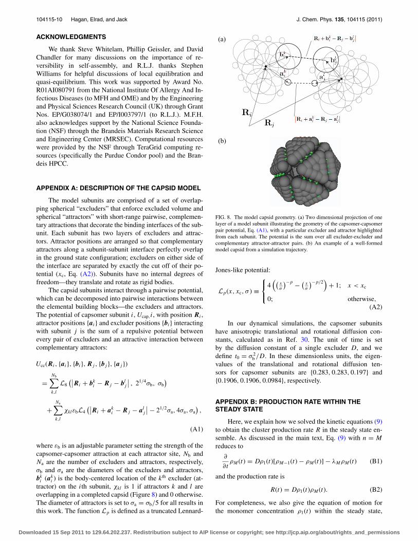
The model subunits are comprised of a set of overlap-ping spherical “excluders” that enforce excluded volume andspherical “attractors” with short-range pairwise, complemen-tary attractions that decorate the binding interfaces of the sub-unit. Each subunit has two layers of excluders and attrac-tors. Attractor positions are arranged so that complementaryattractors along a subunit-subunit interface perfectly overlapin the ground state configuration; excluders on either side ofthe interface are separated by exactly the cut off of their po-tential (xc, Eq. (A2)). Subunits have no internal degrees offreedom—they translate and rotate as rigid bodies.

The capsid subunits interact through a pairwise potential,which can be decomposed into pairwise interactions betweenthe elemental building blocks—the excluders and attractors.The potential of capsomer subunit i, Ucap,i, with position Ri ,attractor positions {ai} and excluder positions {bi} interactingwith subunit j is the sum of a repulsive potential betweenevery pair of excluders and an attractive interaction betweencomplementary attractors:

Ucc(Ri , {ai}, {bi}, Rj , {bj }, {aj })

=Nb∑k,l

L8(∣∣Ri + bk

i − Rj − blj

∣∣ , 21/4σb, σb)

+Na∑k,l

χklεbL4(∣∣Ri + ak

i − Rj − alj

∣∣ − 21/2σa, 4σa, σa),

(A1)

where εb is an adjustable parameter setting the strength of thecapsomer-capsomer attraction at each attractor site, Nb andNa are the number of excluders and attractors, respectively,σb and σa are the diameters of the excluders and attractors,bk

i (aki ) is the body-centered location of the kth excluder (at-

tractor) on the ith subunit, χkl is 1 if attractors k and l areoverlapping in a completed capsid (Figure 8) and 0 otherwise.The diameter of attractors is set to σa = σb/5 for all results inthis work. The function Lp is defined as a truncated Lennard-

(a)

(b)

FIG. 8. The model capsid geometry. (a) Two dimensional projection of onelayer of a model subunit illustrating the geometry of the capsomer-capsomerpair potential, Eq. (A1), with a particular excluder and attractor highlightedfrom each subunit. The potential is the sum over all excluder-excluder andcomplementary attractor-attractor pairs. (b) An example of a well-formedmodel capsid from a simulation trajectory.

Jones-like potential:

Lp(x, xc, σ ) ≡⎧⎨⎩

4((

xσ

)−p − (xσ

)−p/2)

+ 1; x < xc

0; otherwise,(A2)

In our dynamical simulations, the capsomer subunitshave anisotropic translational and rotational diffusion con-stants, calculated as in Ref. 30. The unit of time is setby the diffusion constant of a single excluder D, and wedefine t0 = σ 2

b /D. In these dimensionless units, the eigen-values of the translational and rotational diffusion ten-sors for capsomer subunits are {0.283, 0.283, 0.197} and{0.1906, 0.1906, 0.0984}, respectively.

APPENDIX B: PRODUCTION RATE WITHIN THESTEADY STATE

Here, we explain how we solved the kinetic equations (9)to obtain the cluster production rate R in the steady state en-semble. As discussed in the main text, Eq. (9) with n = M

reduces to

∂

∂tρM (t) = Dρ1(t)[ρM−1(t) − ρM (t)] − λMρM (t) (B1)

and the production rate is

R(t) = Dρ1(t)ρM (t). (B2)

For completeness, we also give the equation of motion forthe monomer concentration ρ1(t) within the steady state,

Downloaded 15 Sep 2011 to 129.64.202.237. Redistribution subject to AIP license or copyright; see http://jcp.aip.org/about/rights_and_permissions

104115-11 Kinetic trapping in self-assembly J. Chem. Phys. 135, 104115 (2011)

which is∂

∂tρ1(t) = MR(t) − 2Dρ1(t)2 + 2λ2ρ2(t)

+M∑

n = 2

[λnρn(t) − Dρ1(t)ρn−1(t)]. (B3)

In the following, we work in the steady state so wesuppress all time dependence of the ρn. Equation (B2)gives ρM = Dρ1/R while Eq. (B1) gives DρM−1 = (R/ρ1)(1 + (λM/Dρ1)). The remaining ρn may then be obtainedinductively since Eq. (9) reduces to D(ρn − ρn−1) = (1/ρ1)[λn+1ρn+1 − λnρn], so that ρn−1 is given in terms of ρm withm ≥ n. For 1 ≤ n ≤ M − 2 we arrive at

Dρn = R

ρ1+ 1

ρ1

M−1∑m= n+1

[λmρm − λm+ 1ρm + 1], (B4)

which allows calculation of all of the ρn, in terms of R, ρ1,and λn.

A simple case is when no unbinding takes place, so thatλm = 0. Then, ρn = ρ1 for all n, and ρT = M(M + 1)ρ1/2.Hence, the production rate for irreversible binding is given byEq. (11).

We now turn to the problem described in the main text,where λm = λ for m ≤ m∗, with λm = 0 for m > m∗. It thenfollows from (B4) that,

ρn ={

RDρ1

, n ≥ m∗,R

Dρ1S(λ̃, m∗ − n), n < m∗,

(B5)

where S(x, n) = (1 − xn+1)/(1 − x) is obtained by summinga geometrical progression and λ̃ = λ/Dρ1. We then sum overn to obtain ρT and eliminate R from the result using

R = Dρ21/S(λ̃, m∗ − 1), (B6)

which follows from Eq. (B5). The result is

(DρT /λ) = (M − m∗)(M + m∗ + 1) + f (λ̃, m∗)

2λ̃S(λ̃, m∗ − 1), (B7)

with

f (λ̃, m) =[m(m + 1) − 2m

∂

∂λ̃+ ∂2

∂λ̃2

]S(λ̃, m). (B8)

[We used∑m

r=1 rxr = x(∂/(∂x))S(x,m) and similarly∑m

r=2r(r − 1)xr = x2(∂2/∂x2)S(x,m).] Dimensional analysisshows that the normalised rate R/R∞ depends only on M ,m∗, and λ/DρT. We, therefore, fix these parameters and solveEq. (B7) numerically for λ̃, obtaining the monomer concen-tration ρ1 = λ/(Dλ̃). The rate R may then be calculated fromEq. (B6), as shown in Fig. 7 and discussed in the main text.

APPENDIX C: BINDING FREE ENERGIES FOR THECAPSID MODEL

We define the free energy change on adding a capsomerto a cluster of size n − 1 (that is, the capsomer binding freeenergy) to be

gb(n) = −T ln

[ρn

ρn−1

css

ρ1

], (C1)

-14

-12

-10

-8

-6

2 3 4 5 6 7 8 9

g b /

k BT

intermediate size, n

-2

-1

0

1

2

3

2 3 4 5 6 7 8 9

Δsc

/ kB

intermediate size, n

(a) (b)

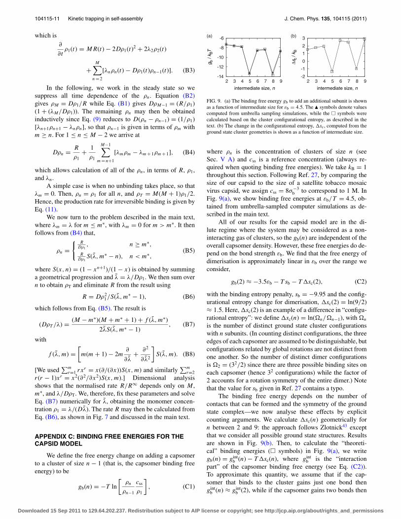
FIG. 9. (a) The binding free energy gb to add an additional subunit is shownas a function of intermediate size for εb = 4.5. The � symbols denote valuescomputed from umbrella sampling simulations, while the � symbols werecalculated based on the cluster configurational entropy, as described in thetext. (b) The change in the configurational entropy, �sc, computed from theground state cluster geometries is shown as a function of intermediate size.

where ρn is the concentration of clusters of size n (seeSec. V A) and css is a reference concentration (always re-quired when quoting binding free energies). We take kB = 1throughout this section. Following Ref. 27, by comparing thesize of our capsid to the size of a satellite tobacco mosaicvirus capsid, we assign css = 8σ−3

b to correspond to 1 M. InFig. 9(a), we show binding free energies at εb/T = 4.5, ob-tained from umbrella-sampled computer simulations as de-scribed in the main text.

All of our results for the capsid model are in the di-lute regime where the system may be considered as a non-interacting gas of clusters, so the gb(n) are independent of theoverall capsomer density. However, these free energies do de-pend on the bond strength εb. We find that the free energy ofdimerisation is approximately linear in εb over the range weconsider,

gb(2) ≈ −3.5εb − T sb − T �sc(2), (C2)

with the binding entropy penalty, sb = −9.95 and the config-urational entropy change for dimerisation, �sc(2) = ln(9/2)≈ 1.5. Here, �sc(2) is an example of a difference in “configu-rational entropy”: we define �sc(n) = ln(�n/�n−1), with �n

is the number of distinct ground state cluster configurationswith n subunits. (In counting distinct configurations, the threeedges of each capsomer are assumed to be distinguishable, butconfigurations related by global rotations are not distinct fromone another. So the number of distinct dimer configurationsis �2 = (32/2) since there are three possible binding sites oneach capsomer (hence 32 configurations) while the factor of2 accounts for a rotation symmetry of the entire dimer.) Notethat the value for sb given in Ref. 27 contains a typo.

The binding free energy depends on the number ofcontacts that can be formed and the symmetry of the groundstate complex—we now analyse these effects by explicitcounting arguments. We calculate �sc(n) geometrically forn between 2 and 9: the approach follows Zlotnick43 exceptthat we consider all possible ground state structures. Resultsare shown in Fig. 9(b). Then, to calculate the “theoreti-cal” binding energies (� symbols) in Fig. 9(a), we writegb(n) = gint

b (n) − T �sc(n), where gintb is the “interaction

part” of the capsomer binding free energy (see Eq. (C2)).To approximate this quantity, we assume that if the cap-somer that binds to the cluster gains just one bond thengint

b (n) ≈ gintb (2), while if the capsomer gains two bonds then

Downloaded 15 Sep 2011 to 129.64.202.237. Redistribution subject to AIP license or copyright; see http://jcp.aip.org/about/rights_and_permissions

104115-12 Hagan, Elrad, and Jack J. Chem. Phys. 135, 104115 (2011)

gintb (n) ≈ gint

b (5). Thus, taking the values of gintb (2)/T = −5.8

and gintb (5)/T = −14.7 obtained from umbrella sampling at

εb/T = 4.5 together with the calculated values of �n, we areable to obtain gb(n) for n ≤ 9, as shown in Fig. 9(a). The fitto the directly measured free energies is excellent.

To obtain the critical capsomer concentration shown inFig. 1, we extrapolate this procedure to a full capsid. We de-fine the capsid free energy,

Gb(20) = −T ln

[ρ20c

19ss

ρ201

]. (C3)

Once this quantity is known, and under the (excellent) as-sumption that the equilibrium state of the system is domi-nated by a combination of monomers and complete capsidswith very few intermediate-sized clusters, the critical cap-somer concentration is obtained by setting ρ1 = 20ρ20, so thathalf of all capsomers are in complete capsids and taking thetotal capsomer density as ρcc = 2ρ1. Hence,

ρcc = 2css

201/19exp

(Gb(20)

19T

). (C4)

From the definitions of gb(n) and �n, the capsid free en-ergy can be written as

Gb(20) =20∑

n=2

gb(n) = −T ln �20 +20∑

n=2

gintb (n), (C5)

where the combinatorial factor associated with the icosahe-dral capsid is �20 = 320/60. We assume that the dependenceof gb on εb is that gint

b (2)/T ≈ −3.5εb/T + sb as discussedabove while gint

b (5)/T ≈ −7εb/T + s ′b since the capsomer

that binds makes two bonds in this case. We also requirean approximation for gint

b (20): adding the final capsomer in-volves adding three new bonds so we approximate this asgint

b (20) ≈ gintb (5) − 3.5εb, including the extra energy gained

from the third bond and neglecting any extra entropy lost.Hence,

Gb(20) ≈ −T log �20 + 9gintb (2) + 10gint

b (5) − 3.5εb, (C6)

and using the numerical values for gintb (2) and gint

b (5)obtained from umbrella sampling at εb/T = 4.5, we ar-rive at Gb(20)/T = −233 − 105(εb/T − 4.5). Finally, us-ing (C4) and (C6) together gives the result for the critical cap-somer concentration shown in Fig. 1(a).

1D. L. D. Caspar and A. Klug, Cold Spring Harbor Symp. Quant. Biol. 27,1 (1962).

2H. Fraenkel-Conrat and R. C. Williams, Proc. Natl. Acad. Sci. U.S.A. 41,690 (1955); A. Klug, Philos. Trans. R. Soc. London, Ser. B 354, 531 (1999);A. Zlotnick, R. Aldrich, J. M. Johnson, P. Ceres, and M. J. Young, Virol-ogy 277, 450 (2000); J. Sun, C. DuFort, M. Daniel, A. Murali, C. Chen,K. Gopinath, B. Stein, M. De, V. M. Rotello, A. Holzenburg, C. Kao, andB. Dragnea, Proc. Natl. Acad. Sci. U.S.A. 104, 1354 (2007).

3A. Zlotnick, J. Mol. Biol. 241, 59 (1994); B. Berger, P. W. Shor, L. Tucker-Kellogg, and J. King, Proc. Natl. Acad. Sci. U.S.A. 91, 7732 (1994);T. Chen, Z. Zhang, and S. C. Glotzer, Proc. Natl. Acad. Sci. U.S.A. 194,717 (2007); H. D. Nguyen, V. S. Reddy, and C. L. Brooks III, Nano Lett.7, 338 (2007).

4M. F. Hagan and D. Chandler, Biophys. J. 91, 42 (2006).5R. L. Jack, M. F. Hagan, and D. Chandler, Phys. Rev. E 76, 021119 (2007).6Y. Yang, R. Meyer, and M. F. Hagan, Phys. Rev. Lett. 104, 258102 (2010).7S. Whitelam, Phys. Rev. Lett. 105, 088102 (2010).8P. Rothemund, Nature (London) 440, 297 (2006).

9S. Sacanna, W. T. M. Irvine, P. M. Chaikin, and D. J. Pine, Nature (London)464, 575 (2010).

10G. M. Whitesides and M. Boncheva, Proc. Natl. Acad. Sci. U.S.A. 99, 4769(2002).

11A. Zlotnick, J. Mol. Biol. 366, 14 (2007).12D. C. Rapaport, Phys. Rev. Lett. 101, 186101 (2008).13O. M. Elrad and M. F. Hagan, Nano Lett. 8, 3850 (2008).14S. Whitelam, E. H. Feng, M. F. Hagan, and P. L. Geissler, Soft Matter 5,

1251 (2009).15H. D. Nguyen, V. S. Reddy, and C. L. Brooks III, Nano Lett. 7, 338

(2007).16A. W. Wilber, J. P. K. Doye, A. A. Louis, E. G. Noya, M. A. Miller, and

P. Wong, J. Chem. Phys. 127, 085106 (2007).17A. W. Wilber, J. P. K. Doye, and A. A. Louis, J. Chem. Phys. 131, 175101

(2009).18D. Klotsa and R. L. Jack, Soft Matter 6, 6294 (2011).19C. Allain, M. Cloitre, and M. Wafra, Phys. Rev. Lett. 74, 1478 (1995).20P. J. Lu, E. Zaccarelli, F. Ciulla, A. B. Schofield, F. Sciortino, and

D. A. Weitz, Nature (London) 453, 499 (2008).21D. Wales, Energy Landscapes (Cambridge University Press, Cambridge,

England, 2004).22F. Baletto, J. P. K. Doye, and R. Ferrando, Phys. Rev. Lett. 88, 075503

(2002).23C. P. Royall, S. R. Williams, T. Ohtsuka, and H. Tanaka, Nature Mater. 7,

556 (2008).24P. Meakin, Phys. Rev. Lett. 51, 1119 (1983).25R. Becker and W. Döring, Ann. Phys. (Leipzig) 416, 719 (1935).26K. Binder and D. Stauffer, Adv. Phys. 25, 343 (1976).27O. Elrad and M. F. Hagan, Phys. Biol. 7, 045003 (2010).28D. Rapaport, J. Johnson, and J. Skolnick, Comput. Phys. Commun.

121–122, 231 (1999); D. Rapaport, Phys. Rev. E 70, 051905 (2004).29A. Branka and D. Heyes, Phys. Rev. E 60, 2381 (1999); D. Heyes and

A. Branka, Mol. Phys. 98, 1949 (2000).30J. G. de la Torre and B. Carrasco, Biopolymers 63, 163 (2002).31The simulations with εb = 4.1 and εb = 4.3 have not completely transi-

tioned into the logarithmic growth phase at this time point. Since the nucle-ation time rises exponentially with decreasing εb (Ref. 38); the transitionto logarithmic growth phase increases in a similar fashion. However, thevariation of yield with respect to εb is robust to this choice of observationtime.

32The maximal interaction energy between subunits is 6εb, so the value of εbat optimal assembly may seem large. However, there is a significant entropypenalty on binding, due to the short length scale of the interactions andtheir orientation-dependence. Thus with εb = 4.5, the binding free energyis approximately gb = −7kBT , as discussed in Appendix C and Fig. 9.

33S. Whitelam and P. L. Geissler, J. Chem. Phys. 127, 154101 (2007).34A. Bhattacharyay and A. Troisi, Chem. Phys. Lett. 458, 210 (2008).35If we had taken Kawasaki dynamics where MC attempted moves involve

single particles, then the diffusion constant of clusters of particles would bevery small when εb is large. The resulting dynamics would not be consistentwith the physical scenario considered here.

36R. J. Baxter, Exactly Solved Models in Statistical Mechanics (Academic,New York, 2002).

37L. Maibaum, Phys. Rev. Lett. 101, 256102 (2008).38M. F. Hagan and O. M. Elrad, Biophys. J. 98, 1065 (2010).39D. Endres and A. Zlotnick, Biophys. J. 83, 1217 (2002).40We note that Y ss

4 depends on the product size cutoff nmax while n4(t) de-pends on the time t , so the comparison between these measurements isnecessarily qualitative, but their respective dependencies on nmax and t areweak and they show similar non-monotonic behaviour.

41In general, such rates depend on the diffusion constants and sizes of therelevant clusters but including such factors does not change any qualitativefeatures of our results.

42In Ref. 5, some of us argued that the poor assembly that often occurs insystem with strong intercomponent bonds is related to the breakdown of acondition that we called local equilibration (our use of this term is simi-lar in spirit to an analogous condition in non-equilibrium thermodynamics(Ref. 59), but the locality that we refer to is the space of cluster configu-rations, rather than in the spatial coordinates of the system). Here, we usethe term “cluster equilibrium” to formulate a closely related condition andwe test the extent to which this condition is correlated with effective self-assembly.

43A. Zlotnick, J. Mol. Biol. 241, 59 (1994).44A. Zlotnick, J. Mol. Recognit. 18, 479 (2005).

Downloaded 15 Sep 2011 to 129.64.202.237. Redistribution subject to AIP license or copyright; see http://jcp.aip.org/about/rights_and_permissions

104115-13 Kinetic trapping in self-assembly J. Chem. Phys. 135, 104115 (2011)

45A. Y. Morozov, R. F. Bruinsma, and J. Rudnick, J. Chem. Phys. 131 (2009).46M. F. Hagan, J. Chem. Phys. 130, 114902 (2009).47A. Bray, Adv. Phys. 43, 357 (1994).48In principle, measurements of Nn,α(t)/Nn,γ (t) in the umbrella-sampled en-

semble may depend on the value of numb, especially if morphologies α andγ have different excluded volumes. In this case the cluster equilibrationcondition would be ill-defined due to cluster-cluster interactions. However,we used a range of values for numb in our simulations and we did not ob-serve any such dependence.

49A. Zlotnick, J. M. Johnson, P. W. Wingfield, S. J. Stahl, and D. Endres,Biochemistry 38, 14644 (1999).

50P. Moisant, H. Neeman, and A. Zlotnick, Biophys. J. 99, 1350 (2010).51B. Sweeney, T. Zhang, and R. Schwartz, Biophys. J. 94, 772 (2008).

52P. Ceres and A. Zlotnick, Biochemistry 41, 11525 (2002).53S. Whitelam, C. Rogers, A. Pasqua, C. Paavola, J. Trent, and P. L. Geissler,

Nano Lett. 9, 292 (2009).54T. P. J. Knowles, C. A. Waudby, G. L. Devlin, S. I. A. Cohen, A. Aguzzi,

M. Vendruscolo, E. M. Terentjev, M. E. Welland, and C. M. Dobson,Science 326, 1533 (2009).

55M. Fandrich, J. Meinhardt, and N. Grigorieff, Prion 3, 89 (2009).56S. P. Katen, S. R. Chirapu, M. G. Finn, and A. Zlotnick, ACS Chem. Biol.

5, 1125 (2010).57S. D. Hicks and C. L. Henley, Phys. Rev. E 74, 031912 (2006).58J. Russo and F. Sciortino, Phys. Rev. Lett. 104, 195701 (2010).59S. de Groot and P. Mazur, Non-equilibrium Thermodynamics (Dover,

Mineola, New York, 1984).

Downloaded 15 Sep 2011 to 129.64.202.237. Redistribution subject to AIP license or copyright; see http://jcp.aip.org/about/rights_and_permissions