MECHANISMS OF ABRUPT CLIMATE CHANGE OF

THE LAST GLACIAL PERIOD

Amy C. Clement1 and Larry C. Peterson1

Received 12 June 2006; revised 24 August 2007; accepted 18 February 2008; published 3 October 2008.

[1] More than a decade ago, ice core records fromGreenland revealed that the last glacial period wascharacterized by abrupt climate changes that recurred onmillennial time scales. Since their discovery, there has beena large effort to determine whether these climate eventswere a global phenomenon or were just confined to theNorth Atlantic region and also to reveal the mechanismsthat were responsible for them. In this paper, we review theavailable paleoclimate observations of abrupt change duringthe last glacial period in order to place constraints onpossible mechanisms. Three different mechanisms are thenreviewed: ocean thermohaline circulation, sea icefeedbacks, and tropical processes. Each mechanism istested for its ability to explain the key features of the

observations, particularly with regard to the abruptness,millennial recurrence, and geographical extent of theobserved changes. It is found that each of thesemechanisms has explanatory strengths and weaknesses,and key areas in which progress could be made inimproving the understanding of their long-term behavior,both from observational and modeling approaches, aresuggested. Finally, it is proposed that a completeunderstanding of the mechanisms of abrupt changerequires inclusion of processes at both low and highlatitudes, as well as the potential for feedbacks betweenthem. Some suggestions for experimental approaches to testfor such feedbacks with coupled climate models are given.

Citation: Clement, A. C., and L. C. Peterson (2008), Mechanisms of abrupt climate change of the last glacial period, Rev. Geophys.,

46, RG4002, doi:10.1029/2006RG000204.

1. INTRODUCTION

[2] Beyond the limited range of historical and instrumen-

tal data, the geologic record has provided abundant evi-

dence of natural climate changes that are both abrupt and

large in magnitude. The most dramatic insights into this

aspect of climate system behavior have come from studies

of ice and sediment cores from the northern North Atlantic.

Ice core results from Greenland were the first to show that

significant changes in regional climate occurred in the past

over time scales of a few years to a few decades at most

[e.g., Alley et al., 1993; Taylor et al., 1993]. The most recent

and perhaps best studied of these events is the Younger

Dryas (YD), an abrupt return to near-glacial temperatures in

the high-latitude North Atlantic lasting roughly a millenni-

um during the last deglaciation (Figure 1). Rapid tempera-

ture excursions were also a characteristic feature of

Greenland climate during the last glacial period according

to ice core records. These excursions, which have come to be

known as Dansgaard-Oeschger or D-O events [Dansgaard et

al., 1984, 1993], recurred roughly every 1500 years and

show up as abrupt warmings over Greenland of as much as

10�C followed by a somewhat more gradual return to cold

glacial conditions (Figure 1). Bond et al. [1993] showed that

D-O events in Greenland are closely matched by sea surface

temperature (SST) changes recorded in high–accumulation

rate sediments in the North Atlantic. Both the abrupt nature

of the cold-to-warm shifts that terminate the cycles and the

recurrence time scale (Figure 1) were found to be similar,

suggesting a linkage between oceanic and cryospheric

processes in this region. In addition, discrete layers of ice-

rafted debris found in subpolar North Atlantic sediments

[Bond et al., 1992], Heinrich events, were deposited period-

ically during the coldest phases of the D-O cycles (Figure 1)

and are thought to have originated from icebergs that came

out of the Hudson Strait [e.g., Hemming, 2004].

[3] Though the amplitude and timing of abrupt climate

change are best defined in the Greenland ice core records

for the last glacial period between about 80,000 and 15,000

years ago, a large number of records from around the world

show evidence of climate events with a similar temporal

behavior [e.g., Broecker and Hemming, 2001; Voelker and

Workshop Participants, 2002; Hemming, 2004]. The chal-

lenge is to determine whether the millennial variability that

clearly shows up as abrupt change in Greenland is actually

related to that at other locations around the globe or has the

same cause. This issue can be addressed from both an1Rosenstiel School of Marine and Atmospheric Science, University of

Miami, Miami, Florida, USA.

Copyright 2008 by the American Geophysical Union.

8755-1209/08/2006RG000204

Reviews of Geophysics, 46, RG4002 / 2008

1 of 39

Paper number 2006RG000204

RG4002

observational and a mechanistic approach. From the obser-

vations, we can ask whether the events in different records

have the same timing, abruptness, and persistence. Many of

the records from the North Atlantic region have been

examined in this context [e.g., Alley et al., 1999; Hemming,

2004], but this is less true for other regions, particularly the

tropics. For the mechanistic approach, the question is

whether there are plausible physical mechanisms that can

link different regions, perhaps at a global scale, and what

drives such mechanisms to produce abrupt changes.

[4] At present, the favored paradigm for explaining the

abrupt climate events seen in ice cores and elsewhere

centers on freshwater input to the high-latitude North

Atlantic and its effect on heat transport into the region via

disruption of the meridional overturning circulation (MOC)

of the Atlantic [e.g., Rooth, 1982; Broecker et al., 1985;

Bond et al., 1993; Rahmstorf, 1995; Alley et al., 1999;

Ganopolski and Rahmstorf, 2001; Knutti et al., 2004]. It is

argued that freshwater discharges into the North Atlantic

Ocean from the surrounding landmasses abruptly weaken

the ocean thermohaline circulation (THC) in the Atlantic

and the delivery of heat from the tropics to the high latitudes

causing cold events in Greenland. The most obvious source

of this fresh water would be from periodic releases of

meltwater derived from the surrounding ice sheets.

[5] A collection of paleochemical data, reviewed in

section 2.1.2, support the premise that the THC has indeed

undergone past changes in its intensity. However, it is not

necessarily clear whether these changes were the cause or

consequence of abrupt climate change. Furthermore, it is

not obvious that THC changes alone can explain the climate

changes recorded both within the North Atlantic and world-

wide [Wunsch, 2006]. Are there other possible mechanisms

that can explain the features of the observations? One such

Figure 1. Comparison of (bottom) North Greenland Ice Core Project (NGRIP) ice core oxygen isotoperecord (a proxy for air temperature) to (top) a typical deep sea sediment oxygen isotope record (a signaldominated by global ice volume). The Mapping Spectral Variability in Global Climate Project(SPECMAP) stack [Imbrie et al., 1984] is a composite record constructed from normalizing andaveraging a number of low-latitude planktic foraminiferal isotope records and is representative of theresolution typically achieved in climate time series based on open ocean marine sediments with low tomoderate sedimentation rates (i.e., less than about 5–8 cm ka�1). The high-resolution NGRIP record[North Greenland Ice Core Project Members, 2004] spans the last 123,000 years and reveals pervasivecentury- to millennial-scale variability not resolvable in typical marine records. The abrupt cooling of theYounger Dryas and the rapid warmings that characterize the well-known Dansgaard-Oeschger interstadialevents are numbered. Heinrich events (labeled H1 to H6) are discrete layers of ice-rafted debris found inmarine sediment cores from a wide swath of the subpolar North Atlantic. They have been interpreted toreflect the episodic discharge of massive numbers of icebergs from the Hudson Strait region.

RG4002 Clement and Peterson: ABRUPT CLIMATE CHANGE MECHANISMS

2 of 39

RG4002

mechanism is a feedback involving sea ice in the North

Atlantic. A number of papers have argued that the capacity

of sea ice to affect climate both through albedo and air-sea

heat exchange and also the ability of sea ice to rapidly

change its distribution make this a good candidate mecha-

nism for driving abrupt climate changes in the North

Atlantic and perhaps worldwide [Gildor and Tziperman,

2003; Timmermann et al., 2003; Kaspi et al., 2004; Li et al.,

2005; Wunsch, 2006; Denton et al., 2005]. Another possi-

bility that has been proposed is that processes in the tropics

play an important role in abrupt climate change [e.g., Cane,

1998; Cane and Clement, 1999; Clement et al., 2001;

Pierrehumbert, 2000; Seager and Battisti, 2007]. On the

basis of the simple reasoning that the tropics are the largest

source of interannual variability in the modern climate

system and are also the main source of heat and water

vapor for the global climate, the tropics would appear to be

critical.

[6] In this paper, we first review and evaluate evidence

for abrupt climate change during the glacial period from the

paleoclimate record. We then review three different sets of

physical mechanisms that have been proposed, thermoha-

line circulation, sea ice feedbacks, and tropical processes, to

determine to what extent each can explain the main tempo-

ral and spatial characteristics of the observations. A final

section suggests a somewhat different approach to under-

standing abrupt climate change by looking at feedbacks that

could link these mechanisms on a global scale.

2. ABRUPT CLIMATE CHANGE OF THE LASTGLACIAL PERIOD: EVIDENCE

[7] The most clear and well-established evidence of

abrupt climate change comes from Greenland ice cores

(Figure 1). That the air temperature and rate of ice accu-

mulation over the summit of the Greenland Ice Sheet can

change abruptly is perhaps surprising in itself, but the more

important issue is whether these climate events appear

outside Greenland with the same dramatic and abrupt

character.

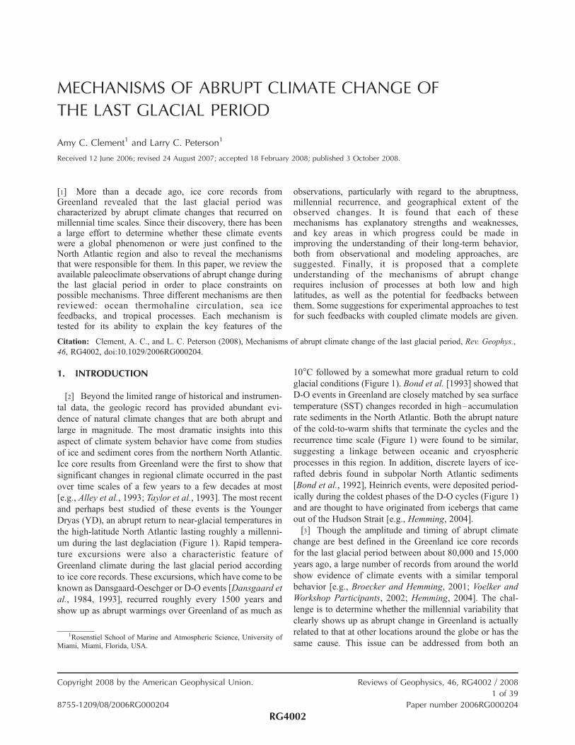
[8] This issue was taken on by Voelker and Workshop

Participants [2002], who made maps of the distribution of

existing paleoclimate records with sufficient resolution in the

time period of marine isotope stage (MIS) 3 to detect D-O

events. Two maps were reconstructed (reproduced here as

Figure 2), one showing the distribution of existing records

with a resolution of <200 years, judged sufficient to identify

D-O-scale events, and the other of records with a resolution

of 200–500 years. The criteria used were that a record must

have seven or more data points during the �1500 year

period of a D-O cycle to be included in the <200 year map

and from five to seven data points per cycle to be included

in the 200–500 year map. The quality of the age model for

each record was also evaluated depending on the nature of

the age control (e.g., 14C, U/Th, and thermoluminescence)

and the number of dated levels within the time period of

MIS 3. One of the most striking aspects of the Voelker and

Workshop Participants [2002] maps, but especially of the

<200 year map, is that while the analysis indicates that D-O

correlative events can be seen in regions all over the globe,

including the tropics and Southern Hemisphere, there is an

extremely disproportionate coverage of the North Atlantic,

with enormous spatial gaps throughout the rest of the globe.

[9] Before going into our review of the records, we wish

to point out a few issues for the reader to be aware of. First,

we have not tried to apply a strict or concise definition of

abrupt climate change in this paper. Examples of abrupt

change from in and around Greenland (Figure 1) include the

Younger Dryas cold event and the D-O events of the last

glacial, as well as the Heinrich events recorded in North

Atlantic sediments. These events all exhibit transitions that

occur on decadal to centennial time scales and have recur-

rence time scales of roughly millennia. There is little reason

to expect that they will look identical in different records

because it is not clear to what extent these different types of

events are actually analogous to each other and also because

Figure 2. Spatial distribution of (top) sites with resolutionof 1–200 years during MIS 3 and (bottom) sites withresolution of 200–500 years. Solid circles indicate siteswith evidence of clear D-O-type climate oscillations, whileopen circles indicate locations where D-O cyclicity isunclear or absent. Reprinted from Voelker and WorkshopParticipants [2002], copyright 2002, with permission fromElsevier.

RG4002 Clement and Peterson: ABRUPT CLIMATE CHANGE MECHANISMS

3 of 39

RG4002

different proxies are likely to record even the same event

differently [e.g., Hemming, 2004]. Another issue that con-

tinually plagues the evaluation of abrupt change comes from

limitations of the ability to date records precisely. In ice

cores, for example, annual layer counting is used to provide

absolute dating in calendar years down to a depth where

compaction or basal deformation blurs or eliminates the

visual layering [e.g., Alley et al., 1997]. Below that, dating

is usually based on a combination of techniques, including

ice flow models, the identification of previously dated time

markers (e.g., volcanic deposits), and synchronization to

variations in the Earth’s orbital parameters. In contrast,

marine sediments typically are dated using radiocarbon

methods back to approximately 45,000 years ago and then

calibration of the measured 14C ages to the calendar scale is

relied upon [e.g., Kitagawa and van der Plicht, 1998;

Hughen et al., 2004a]. Foraminiferal oxygen isotope strat-

igraphies correlated to an orbitally tuned standard [e.g.,

Imbrie et al., 1984] typically provide age control in older

sequences. Speleothems and lake sediments each have their

own dating methods and issues as well. Furthermore, differ-

ences in the temporal resolution between the different types

of archives can dramatically affect the ability to correlate the

respective climate proxies. The temporal resolution allowed

by ice cores is often an order of magnitude or more better

than what can be achieved in marine sediments, while

archives like speleothems may provide high temporal res-

olution but can experience discontinuous growth. Wunsch

[2006] has raised the above issues, suggesting that they

present serious limitations to the ability to determine wheth-

er millennial variability is correlated in records around the

globe.

[10] Thus, the definition of abrupt climate change will

remain somewhat vague in this paper, and we will focus on

the last glacial stage and temporal features in records that

include decadal to centennial-time scale transitions with

millennial-time scale recurrence. Where possible, the

detailed timing, abruptness, and persistence of specific

events at specific locations will be evaluated, and the

records will be interpreted to determine to what extent the

climate change or the proxy response is abrupt, but issues of

proxy calibration and age control will still be a severe

limitation.

[11] A final point we wish to make is that since our focus

is on mechanisms, the goal of this section is not so much a

comprehensive review of all the available climate records

that show abrupt change but rather an identification of the

records that place key constraints on the possible mecha-

nisms. A more comprehensive review is given by the

National Research Council Committee on Abrupt Climate

Change [2002].

2.1. High Northern Latitudes

2.1.1. Records of Surface Change[12] In many respects, the ice core records from Green-

land have become the de facto ‘‘type-section’’ for late

Pleistocene climate change, in that they serve as the

measuring stick against which other climate records are

inevitably compared. This is perhaps not surprising given

their continuity, their intensive study at high resolution, and

the simple fact that they were the among the first archives to

yield clear evidence of climate changes that were startlingly

rapid, including the aforementioned D-O events as well as

the Younger Dryas (Figure 1). Furthermore, the long Green-

land Ice Core Project (GRIP) [Dansgaard et al., 1993] and

Greenland Ice Sheet Project 2 (GISP2) [Grootes et al.,

1993] ice core records are virtually identical back to about

90,000 years B.P., giving confidence in their signals. The

new North Greenland Ice Core Project ice core has extended

the Greenland air temperature record back to about 123,000

years B.P. [North Greenland Ice Core Project Members,

2004] with the d18Oice data over its length presented as

50 year mean values. In younger intervals where the annual

layering is readily visible, large temperature changes, such

as the warming experienced at the end of the Younger

Dryas, have been shown to occur within decades or less

[Alley et al., 1993; Taylor et al., 1993]. The rapid warmings

in Greenland are also accompanied by equally abrupt

increases (50–100%) in the rate of ice accumulation [Alley

et al., 1993; Cuffey and Clow, 1997]. The D-O events in

Greenland recur on an approximately 1500 year time scale,

though this is an average value [Schulz, 2002; Rahmstorf,

2003], and the recurrence interval can vary greatly from

event to event (Figure 1).

[13] The first marine evidence for abrupt changes appar-

ently synchronous with those in Greenland came from

relatively high–accumulation rate sediment cores in the

subpolar North Atlantic. Here, records of SST, based on

abundance changes in a temperature-sensitive foraminifer,

showed that the Younger Dryas and D-O climate events in

Greenland were matched by corresponding SST changes of

at least 5�C [Bond et al., 1992, 1993]. Similar estimates

have been derived by Elliot et al. [2002], who identified

SST variations across D-O events of 3�C–5�C on Rockall

Plateau. At the high-latitude locations of these investiga-

tions, SST variations can most easily be explained by north-

south shifts in the position of the Polar Front. The initial

studies by Bond et al. [1992, 1993] were also able to

establish the temporal relationship between the temperature

oscillations in Greenland and Heinrich events, discrete

layers of ice-rafted debris (IRD) found in North Atlantic

sediments [Heinrich, 1988] inferred by Broecker et al.

[1992] and Hemming [2004] to reflect massive discharges

of icebergs from the Hudson Strait region. Heinrich events,

the timing of which is indicated in Figure 1, occurred during

the coldest intervals of the last glacial at roughly 6000 year

intervals. An extensive review of the origin, distribution,

and timing of Heinrich event layers is given by Hemming

[2004].

[14] In the subtropical North Atlantic, Sachs and Lehman

[1999] presented a proxy SST record from the Bermuda

Rise (33�N) for the time period between 60,000 and 30,000

years B.P. that clearly showed that abrupt temperature

changes associated with the D-O events in Greenland and

in the surrounding subpolar waters were experienced at this

more southerly location (see Figure 3). Their record, based

RG4002 Clement and Peterson: ABRUPT CLIMATE CHANGE MECHANISMS

4 of 39

RG4002

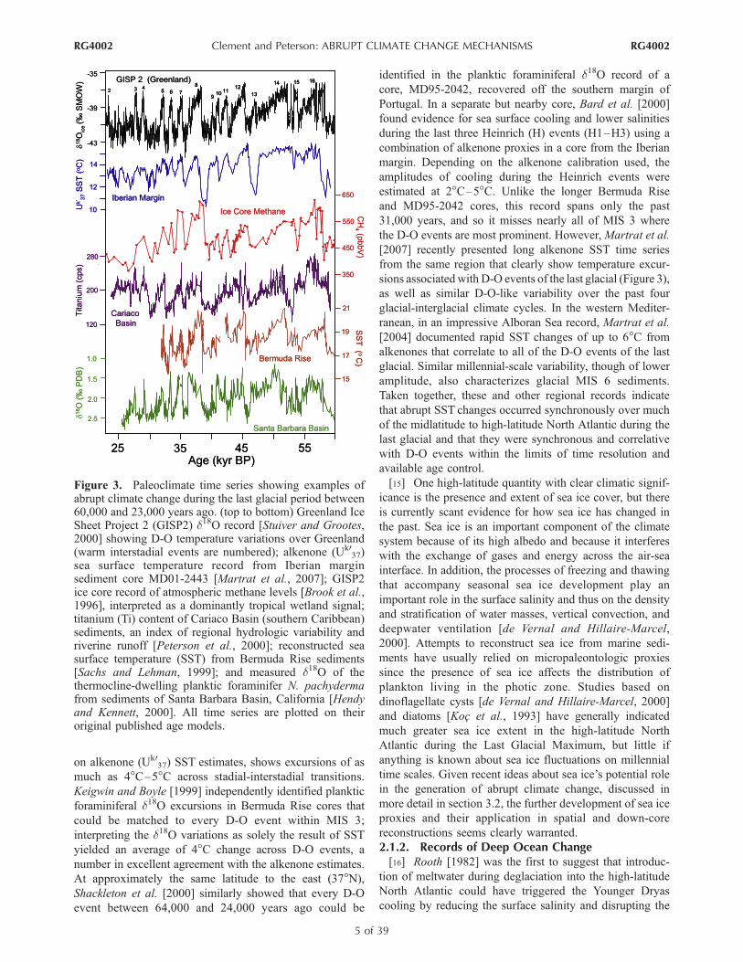
on alkenone (Uk037) SST estimates, shows excursions of as

much as 4�C–5�C across stadial-interstadial transitions.

Keigwin and Boyle [1999] independently identified planktic

foraminiferal d18O excursions in Bermuda Rise cores that

could be matched to every D-O event within MIS 3;

interpreting the d18O variations as solely the result of SST

yielded an average of 4�C change across D-O events, a

number in excellent agreement with the alkenone estimates.

At approximately the same latitude to the east (37�N),Shackleton et al. [2000] similarly showed that every D-O

event between 64,000 and 24,000 years ago could be

identified in the planktic foraminiferal d18O record of a

core, MD95-2042, recovered off the southern margin of

Portugal. In a separate but nearby core, Bard et al. [2000]

found evidence for sea surface cooling and lower salinities

during the last three Heinrich (H) events (H1–H3) using a

combination of alkenone proxies in a core from the Iberian

margin. Depending on the alkenone calibration used, the

amplitudes of cooling during the Heinrich events were

estimated at 2�C–5�C. Unlike the longer Bermuda Rise

and MD95-2042 cores, this record spans only the past

31,000 years, and so it misses nearly all of MIS 3 where

the D-O events are most prominent. However, Martrat et al.

[2007] recently presented long alkenone SST time series

from the same region that clearly show temperature excur-

sions associated with D-O events of the last glacial (Figure 3),

as well as similar D-O-like variability over the past four

glacial-interglacial climate cycles. In the western Mediter-

ranean, in an impressive Alboran Sea record, Martrat et al.

[2004] documented rapid SST changes of up to 6�C from

alkenones that correlate to all of the D-O events of the last

glacial. Similar millennial-scale variability, though of lower

amplitude, also characterizes glacial MIS 6 sediments.

Taken together, these and other regional records indicate

that abrupt SST changes occurred synchronously over much

of the midlatitude to high-latitude North Atlantic during the

last glacial and that they were synchronous and correlative

with D-O events within the limits of time resolution and

available age control.

[15] One high-latitude quantity with clear climatic signif-

icance is the presence and extent of sea ice cover, but there

is currently scant evidence for how sea ice has changed in

the past. Sea ice is an important component of the climate

system because of its high albedo and because it interferes

with the exchange of gases and energy across the air-sea

interface. In addition, the processes of freezing and thawing

that accompany seasonal sea ice development play an

important role in the surface salinity and thus on the density

and stratification of water masses, vertical convection, and

deepwater ventilation [de Vernal and Hillaire-Marcel,

2000]. Attempts to reconstruct sea ice from marine sedi-

ments have usually relied on micropaleontologic proxies

since the presence of sea ice affects the distribution of

plankton living in the photic zone. Studies based on

dinoflagellate cysts [de Vernal and Hillaire-Marcel, 2000]

and diatoms [Koc et al., 1993] have generally indicated

much greater sea ice extent in the high-latitude North

Atlantic during the Last Glacial Maximum, but little if

anything is known about sea ice fluctuations on millennial

time scales. Given recent ideas about sea ice’s potential role

in the generation of abrupt climate change, discussed in

more detail in section 3.2, the further development of sea ice

proxies and their application in spatial and down-core

reconstructions seems clearly warranted.

2.1.2. Records of Deep Ocean Change[16] Rooth [1982] was the first to suggest that introduc-

tion of meltwater during deglaciation into the high-latitude

North Atlantic could have triggered the Younger Dryas

cooling by reducing the surface salinity and disrupting the

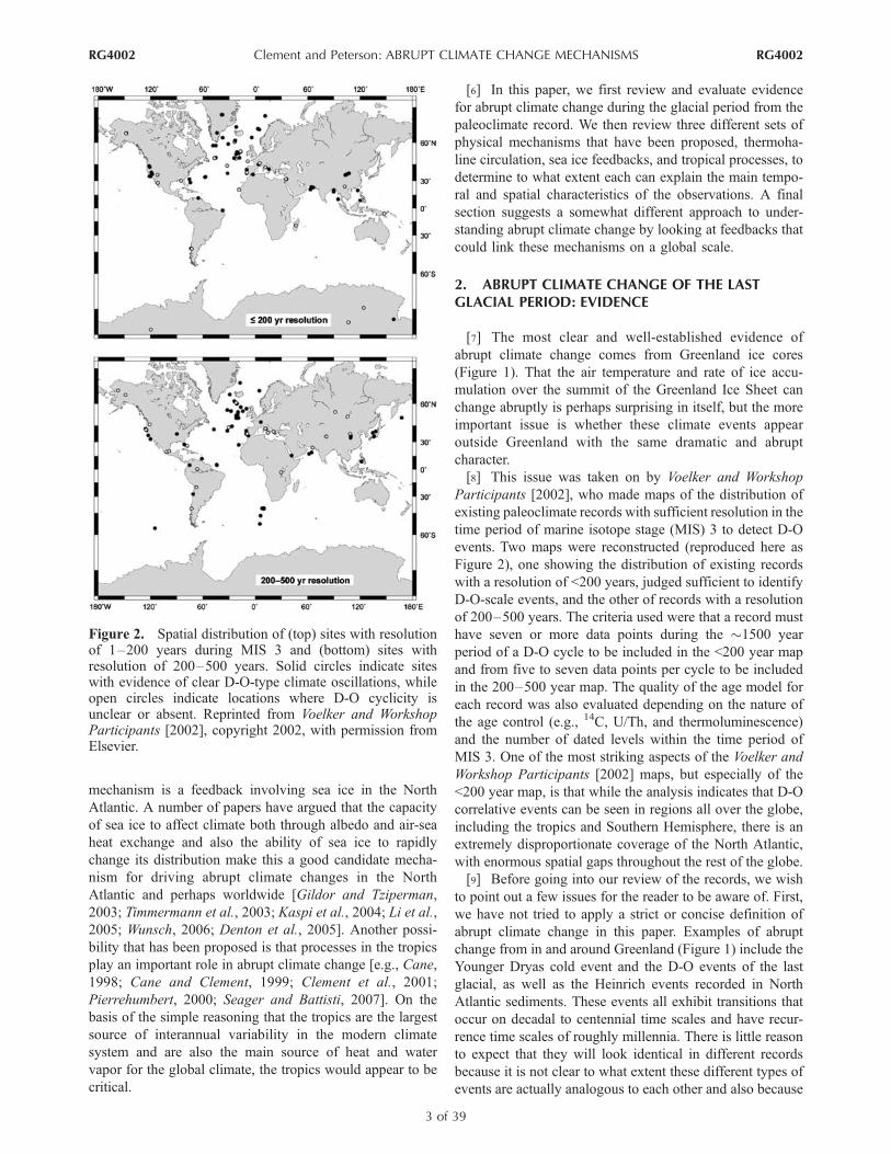
Figure 3. Paleoclimate time series showing examples ofabrupt climate change during the last glacial period between60,000 and 23,000 years ago. (top to bottom) Greenland IceSheet Project 2 (GISP2) d18O record [Stuiver and Grootes,2000] showing D-O temperature variations over Greenland(warm interstadial events are numbered); alkenone (Uk0

37)sea surface temperature record from Iberian marginsediment core MD01-2443 [Martrat et al., 2007]; GISP2ice core record of atmospheric methane levels [Brook et al.,1996], interpreted as a dominantly tropical wetland signal;titanium (Ti) content of Cariaco Basin (southern Caribbean)sediments, an index of regional hydrologic variability andriverine runoff [Peterson et al., 2000]; reconstructed seasurface temperature (SST) from Bermuda Rise sediments[Sachs and Lehman, 1999]; and measured d18O of thethermocline-dwelling planktic foraminifer N. pachydermafrom sediments of Santa Barbara Basin, California [Hendyand Kennett, 2000]. All time series are plotted on theiroriginal published age models.

RG4002 Clement and Peterson: ABRUPT CLIMATE CHANGE MECHANISMS

5 of 39

RG4002

thermohaline circulation. Broecker et al. [1985] further

developed this idea into the THC model that prevails

today, with the rapid warmings (interstadials) and coolings

(stadials) of the North Atlantic region interpreted to reflect

a vigorous and weak THC, respectively. Considerable

evidence exists to support the notion that the THC has

varied with time. This evidence comes primarily in the form

of sediment proxies that reflect either the paleonutrient

content of the deepwater column or in some way record

the strength or intensity of the deep flow. During the

Younger Dryas cooling, for example, d13C and Cd/Ca data

from benthic foraminifera suggest that an older and more

nutrient-rich water mass of probable southern origins

replaced North Atlantic Deep Water (NADW) [Boyle and

Keigwin, 1987; Keigwin et al., 1991; Marchitto et al.,

1998]. This inference is supported by measurements of

grain size in the sortable silt fraction of several North

Atlantic cores [e.g., McCave et al., 1995; Manighetti and

McCave, 1995], with reduced grain size interpreted to

indicate a weakening of deep currents associated with lower

North Atlantic Deep Water.

[17] On the basis of a collection of paleoceanographic

proxies from the North Atlantic, Clark et al. [2002] argued

that the THC has abruptly shifted between different

‘‘modes’’ of operation, which include a modern mode

(strong overturning), a glacial mode (weak and shallower

overturning), and a Heinrich mode (an essentially complete

shutdown). In each of these modes, the sources of the

deepwater masses in the North Atlantic vary geographically.

Recent measurements of sedimentary 231Pa/230Th, inter-

preted as a kinematic proxy for the strength of the THC,

would seem to support the interpretation of multiple modes.

Using 231Pa/230Th in sediments from a core near Bermuda

Rise, McManus et al. [2004] have argued that the meridi-

onal overturning of the Atlantic was nearly or completely

eliminated during the last of the massive iceberg discharge

events of the glacial, Heinrich 1 (H1) (�17,500 years ago),

and declined sharply during the Younger Dryas event. In a

separate study using 231Pa/230Th in a core from the Iberian

margin, Gherardi et al. [2005] found that similar reductions

in the MOC could be inferred at this location over the last

20,000 years, the same time interval spanned in theMcManus

et al. [2004] study. Since 231Pa/230Th can potentially be

biased by variations in particle flux and composition, the

observation of similar 231Pa/230Th patterns in different

sedimentary environments is important because it tends to

confirm that the ratio changes indeed record basinwide

changes in deep circulation. However, timing differences

between the two locations (i.e., western and eastern North

Atlantic basins) indicate that the story of 231Pa/230Th may

be more complicated than first thought. Broecker and

Barker [2007], for example, note that the apparent reduction

in deepwater production during the H1 event in the core

studied by Gherardi et al. [2005] occurred more than a

thousand years later than that found by McManus et al.

[2004]. This suggests differences between renewal rates in

the deep eastern and western basins, and perhaps location-

dependent differences between shallow and deep overturn-

ing must be factored into understanding the history of the

MOC.

[18] The paradigm of fresh water (meltwater) stratifying

the surface ocean in the high-latitude North Atlantic and

serving as the driver for THC changes and abrupt climate

events is largely based on a reconstructed sequence of

events linked in time to the Younger Dryas cooling, specif-

ically the sudden eastward diversion of fresh water from

glacial Lake Agassiz directly into the North Atlantic via the

Great Lakes–St. Lawrence River system at the beginning of

the Younger Dryas [e.g., Clark et al., 2001; Teller et al.,

2002]. However, open issues remain, and a number of

studies have raised questions about the existence and

reported timing of freshwater diversion at the time of the

Younger Dryas [e.g., Lowell et al., 2005; Teller et al., 2005;

Moore, 2005; Broecker, 2006a]. Many of these concerns

seem to have been addressed in a recent study that applied

new proxies for freshwater sources (DMg/Ca, U/Ca, and87Sr/86Sr) to planktonic foraminifera recovered from sedi-

ments at the mouth of the St. Lawrence estuary [Carlson et

al., 2007]. These new measurements seem to confirm that

routing of fresh water from western Canada to the St.

Lawrence River did indeed occur at the start of the Younger

Dryas, and they allow for calculation of an initial base

increase in freshwater flux of 0.06 ± 0.02 sverdrups (Sv)

(where 1 Sv = 106 m3 s�1) and a maximum discharge of

0.12 ± 0.02 Sv. This estimate of initial discharge flux is in

good agreement with an earlier flux estimate of 0.07 Sv

made by Licciardi et al. [1999] for the Younger Dryas but is

considerably smaller than estimates made by Hemming

[2004] for freshwater inputs to the North Atlantic during

Heinrich events (0.15–0.3 Sv over 500 years and 1.0 Sv if

over 1 year, see Table 1).

[19] Though it is now reasonably well established that

variations in the THC accompanied the Younger Dryas and

at least the last of the Heinrich events, it is less clear

whether the abrupt D-O events recorded in Greenland ice

and elsewhere in surface records of the North Atlantic were

all accompanied by similar THC changes. Longer sediment

time series of some of the same paleonutrient proxies (e.g.,

benthic foraminiferal d13C) suggest that deepwater changescharacterized earlier Heinrich events and at least some of

the D-O events [e.g., Oppo and Lehman, 1995; Charles et

al., 1996; Keigwin and Boyle, 1999; Curry et al., 1999;

Hagen and Keigwin, 2002]. However, it is difficult to point

to any single record that provides compelling and unam-

biguous evidence of a direct, one-to-one link between THC

variations and all of the abrupt events of the last glacial. To

some extent, this likely reflects the fact that the three-

dimensional nature of the ocean’s deep circulation makes

it inherently more complex to reconstruct than the past

properties of the surface ocean, which is essentially a two-

dimensional problem. Evidence of past changes in the

shallow meridional overturning may possibly be missed in

deeper records and vice versa. Elliot et al. [2002], for

example, in their study of two sediment cores from off

southeastern Greenland and Rockall Plateau used benthic

d13C variations to infer that Heinrich events were related to

RG4002 Clement and Peterson: ABRUPT CLIMATE CHANGE MECHANISMS

6 of 39

RG4002

large-scale reductions in deepwater production but found

that the cold stadial events in between were not associated

with recognizable decreases in the MOC at least at the water

depth of the two core sites (�2000 m). In contrast, Keigwin

and Boyle [1999] reported d13C records from water depths

close to 4600 m at Bermuda Rise that look more D-O-like in

nature for at least a portion of MIS 3 but show no clear

indication of an amplified Heinrich-type signal. Vautravers

et al. [2004] present a benthic d13C record from a Blake

Outer Ridge site at 3480 m water depth; at this location,

changes in the deepwater d13C proxy appear to be associ-

ated with some, but not all, D-O events. Although not in

itself a record of MOC changes, Hill et al. [2006] presented

evidence from a Gulf of Mexico core that earlier glacial

episodes of Laurentide Ice Sheet meltwater outflow from

the Mississippi River fail to match the timing expected if

meltwater diversion, in a situation analogous to the

Younger Dryas excursion, is to explain the abrupt events

during MIS 3.

[20] One of the more intriguing studies that addresses the

relationship between the MOC and abrupt climate events is

that of Kissel et al. [1999], who compiled bulk magnetic

parameter data from a suite of seven North Atlantic cores

ranging in latitude from 67�N to 33�N and covering

different water depths. Short-term variations in the magnetic

properties could be well correlated between cores and were

interpreted by Kissel et al. to reflect changes in the transport

efficiency of the magnetic particles by deep currents.

Though the age control is at least partly based on wiggle

matching, there is a fairly remarkable match between

magnetic parameters and the Greenland temperature record,

interpreted to indicate a weakening of current strength and

particle transport during cold stadial and Heinrich events.

[21] In some cases, sampling and resolution issues

complicate the interpretation of records. For example,

Piotrowski et al. [2005] used neodymium isotopes, which

can be applied as a conservative tracer of deepwater end-

members, to reconstruct circulation changes from cores in

the Cape Basin of the South Atlantic (�40�S). Their recordnicely shows that changes in the relative proportions of

northern-sourced North Atlantic Deep Water and southern-

sourced Antarctic Bottom Water occurred at this location

during some of the longer interstadial events of MIS 3 (e.g.,

interstadials 8, 12, and 14). However, the temporal resolu-

tion of the record is insufficient to show whether this

linkage persists for the shorter D-O events as well. In other

cases, the resolution is sufficient, but the time interval

studied does not encompass the entire glacial. Skinner and

Elderfield [2007], for example, recently presented the first

benthic foraminiferal Mg/Ca record with the resolution

necessary to see D-O variations in deepwater temperature.

Their record, from 2637 m water depth on the Iberian

margin, indicates a positive correlation between deepwater

temperature change and Greenland temperatures but only

spans the relatively short interval of Greenland interstadials

8 to 12 (�36,000 through 50,000 years ago) at present.

Although abundant data exist to support the hypothesis that

the Atlantic MOC was weaker during the Younger Dryas

and perhaps weaker still during earlier Heinrich events, it

can be argued that unequivocal evidence for a direct

relationship between D-O events and the MOC has yet to

emerge.

2.2. High Southern Latitudes

[22] Like their Greenland counterparts, Antarctic ice

cores contain probably the best and most complete records

of climate in the high-latitude Southern Hemisphere. How-

ever, slower ice accumulation rates tend to result in less

highly resolved records that make it more difficult to assess

the nature of millennial-scale climate events and especially

their timing relative to high-latitude North Atlantic changes.

Antarctic temperature variations (inferred from d18O and dDrecords) show a pattern of more gradual and less pro-

nounced warming and cooling events over the same period

that Greenland ice records the abrupt D-O events of the last

glacial. Blunier et al. [1998], nevertheless, identified an out-

of-phase behavior between temperature in the Byrd and

Vostok (Antarctic) and Greenland ice cores over several of

the longer-lasting interstadials (D-O events 8 and 12) and

argued that this interhemispheric coupling was the result of

THC variations. Underlying this interpretation is the prem-

ise that a vigorous THC draws heat from the Southern

Ocean and that a weakening or collapse of the meridional

overturning results in cooling of the North Atlantic and a

concomitant warming in the Antarctic region, a mechanism

that has come to be known as the ‘‘bipolar seesaw’’

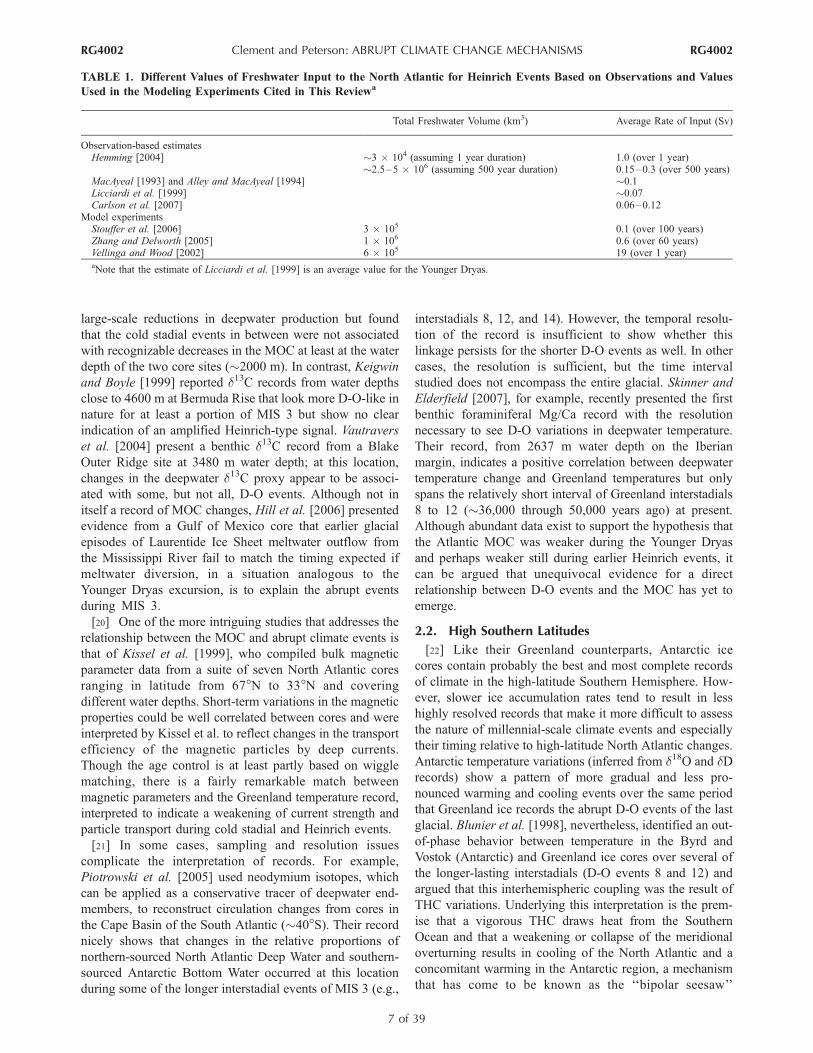
TABLE 1. Different Values of Freshwater Input to the North Atlantic for Heinrich Events Based on Observations and Values

Used in the Modeling Experiments Cited in This Reviewa

Total Freshwater Volume (km3) Average Rate of Input (Sv)

Observation-based estimatesHemming [2004] �3 � 104 (assuming 1 year duration) 1.0 (over 1 year)

�2.5–5 � 106 (assuming 500 year duration) 0.15–0.3 (over 500 years)MacAyeal [1993] and Alley and MacAyeal [1994] �0.1Licciardi et al. [1999] �0.07Carlson et al. [2007] 0.06–0.12

Model experimentsStouffer et al. [2006] 3 � 105 0.1 (over 100 years)Zhang and Delworth [2005] 1 � 106 0.6 (over 60 years)Vellinga and Wood [2002] 6 � 105 19 (over 1 year)aNote that the estimate of Licciardi et al. [1999] is an average value for the Younger Dryas.

RG4002 Clement and Peterson: ABRUPT CLIMATE CHANGE MECHANISMS

7 of 39

RG4002

[Crowley, 1992; Stocker et al., 1992; Stocker, 1998;

Broecker, 1998]. On the basis of further analysis of the

Byrd ice core, Blunier and Brook [2001] subsequently

argued that at least seven Antarctic warming events over

the glacial were matched by Greenland cooling, providing

further support for the so-called bipolar temperature seesaw.

Most recently, study of the new European Programme for Ice

Coring in Antarctica (EPICA) DronningMaud Land (EDML)

ice core has yielded an Antarctic climate record with a

resolution comparable to Greenland [EPICA Community

Members, 2006]. With the enhanced resolution of the new

oxygen isotope record from EDML, it is now clearly

more evident that a one-to-one coupling exists between all

Antarctic warm events and their cold stadial counterparts

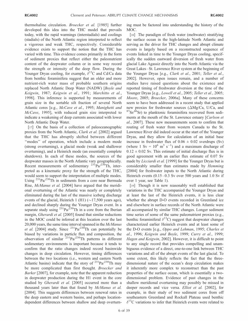
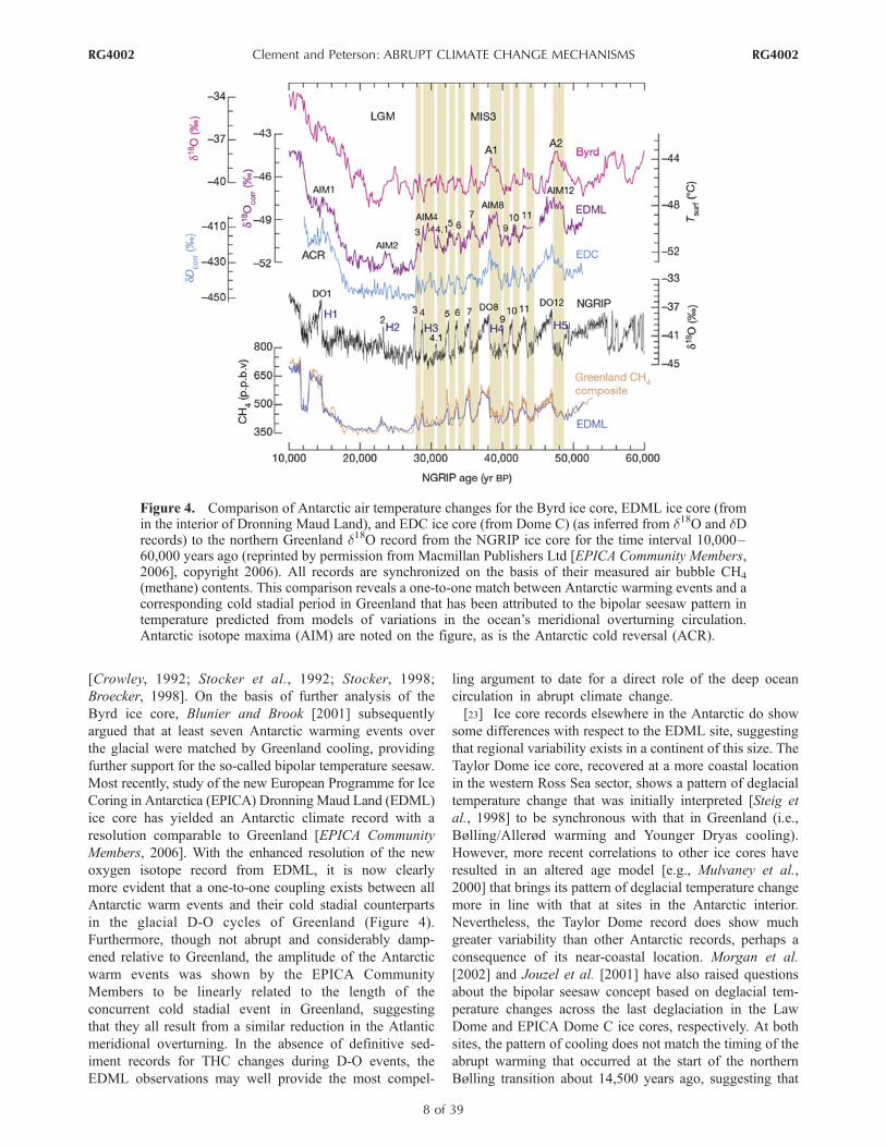
in the glacial D-O cycles of Greenland (Figure 4).

Furthermore, though not abrupt and considerably damp-

ened relative to Greenland, the amplitude of the Antarctic

warm events was shown by the EPICA Community

Members to be linearly related to the length of the

concurrent cold stadial event in Greenland, suggesting

that they all result from a similar reduction in the Atlantic

meridional overturning. In the absence of definitive sed-

iment records for THC changes during D-O events, the

EDML observations may well provide the most compel-

ling argument to date for a direct role of the deep ocean

circulation in abrupt climate change.

[23] Ice core records elsewhere in the Antarctic do show

some differences with respect to the EDML site, suggesting

that regional variability exists in a continent of this size. The

Taylor Dome ice core, recovered at a more coastal location

in the western Ross Sea sector, shows a pattern of deglacial

temperature change that was initially interpreted [Steig et

al., 1998] to be synchronous with that in Greenland (i.e.,

Bølling/Allerød warming and Younger Dryas cooling).

However, more recent correlations to other ice cores have

resulted in an altered age model [e.g., Mulvaney et al.,

2000] that brings its pattern of deglacial temperature change

more in line with that at sites in the Antarctic interior.

Nevertheless, the Taylor Dome record does show much

greater variability than other Antarctic records, perhaps a

consequence of its near-coastal location. Morgan et al.

[2002] and Jouzel et al. [2001] have also raised questions

about the bipolar seesaw concept based on deglacial tem-

perature changes across the last deglaciation in the Law

Dome and EPICA Dome C ice cores, respectively. At both

sites, the pattern of cooling does not match the timing of the

abrupt warming that occurred at the start of the northern

Bølling transition about 14,500 years ago, suggesting that

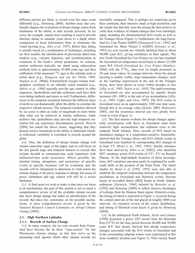
Figure 4. Comparison of Antarctic air temperature changes for the Byrd ice core, EDML ice core (fromin the interior of Dronning Maud Land), and EDC ice core (from Dome C) (as inferred from d18O and dDrecords) to the northern Greenland d18O record from the NGRIP ice core for the time interval 10,000–60,000 years ago (reprinted by permission from Macmillan Publishers Ltd [EPICA Community Members,2006], copyright 2006). All records are synchronized on the basis of their measured air bubble CH4

(methane) contents. This comparison reveals a one-to-one match between Antarctic warming events and acorresponding cold stadial period in Greenland that has been attributed to the bipolar seesaw pattern intemperature predicted from models of variations in the ocean’s meridional overturning circulation.Antarctic isotope maxima (AIM) are noted on the figure, as is the Antarctic cold reversal (ACR).

RG4002 Clement and Peterson: ABRUPT CLIMATE CHANGE MECHANISMS

8 of 39

RG4002

considerable spatial heterogeneity in the record of temper-

ature exists. Finally, while the amplitude of climate change

in the Antarctic is generally dampened at best relative to

events in Greenland, rapid shifts in climate are not undoc-

umented for the region. At the site of the Siple Dome ice

core, near the edge of the Ross Ice Shelf, Taylor et al.

[2004] documented a dramatic rise in air temperature of

�6�C about 22,000 years ago. This sharp temperature

increase apparently occurred within a few decades and has

no obvious counterpart in Greenland nor within other

Antarctic sites.

[24] Land-based records of climate change from the

southern high latitudes are few and far between and suffer

from age controversies and a resolution generally too low to

preserve millennial-scale events, let alone abrupt changes.

In addition, few available land-based records extend beyond

the late glacial, and none that we can find are suitable for

revealing evidence of D-O equivalent events. Even records

that span the general time interval of the Younger Dryas

event are equivocal. On the basis of radiocarbon dating of

glacial deposits in the Southern Alps of New Zealand,

Denton and Hendy [1994] and Lowell et al. [1995] argued

for a glacial advance during the Younger Dryas in New

Zealand. South Island pollen records suggest that increased

moisture is more strongly indicated than cooling at this time

[Fitzsimons, 1997; Singer et al., 1998], while Turney et al.

[2003] interpreted pollen records from both the North and

South islands to indicate warming and an increase in

westerly airflow during the interval correlative with the

Younger Dryas chronozone. A more recent speleothem

study of northern South Island sites by Williams et al.

[2005] concluded that the Younger Dryas stadial was not

well defined in New Zealand and that at the millennial scale

a more convincing case can be made for an asymmetric

climate response between the two hemispheres rather than a

synchronous one. In southern South America, records are

similarly contradictory. In the midlatitudes of southern

Chile, glacial deposits have been used to argue for inter-

hemispheric synchrony in temperature during deglaciation

[e.g., Lowell et al., 1995]. In contrast, pollen records from

the same general area reveal no evidence for a cooling at the

time of the Younger Dryas [Bennett et al., 2000].

[25] Southern Hemisphere marine records are equally

scarce. In a sediment core off New Zealand, Pahnke and

Zahn [2005] found benthic foraminiferal d13C evidence for

increases in intermediate water formation linked to Heinrich

events and periods of inferred minimum NADW production

in the North Atlantic. In the same core from Chatham Rise,

Sachs and Anderson [2005] identified coincident episodes

of increased surface productivity from concentration

changes in sedimentary biomarkers diagnostic of coccoli-

thophorids and diatoms. The sampling interval in both

studies averaged about 200 years, which combined with

bioturbation, makes it difficult to judge abruptness. There is

no clear evidence of D-O-like excursions in either record.

Off the Chilean continental margin, alkenone-based esti-

mates of SST made by Lamy et al. [2004] show evidence of

local millennial-scale SST changes of 2�C–3�C between

8000 and 50,000 years ago and a timing similar to Antarctic

records, with warming of surface waters off Chile matching

the Antarctic warmings that coincide with Heinrich events.

Again, a sampling interval averaging 300 years makes it

impractical to judge abruptness. More recently, Kaiser et al.

[2005] extended the alkenone SST record of Lamy et al.

[2004] back to 70,000 years and presented an improved age

model for this site, which together reinforce the conclusion

that millennial-scale SST variability at this midlatitude

(41�S) location exhibits a distinctly Antarctic behavior.

[26] In summary, the relatively small number of existing

high-latitude climate records from the Southern Hemisphere

reveal potentially complicated regional patterns of climate

change, and few, in truth, possess the length, temporal

resolution, and age control needed to provide hard con-

straints on changes occurring around the time of the abrupt

events in Greenland. The most obvious exception is the

remarkable new EDML ice core record from the Antarctic

(Figure 4), which appears to show a dampened but out-of-

phase temperature pattern for all D-O events consistent with

the bipolar seesaw hypothesis. Regardless of what one may

conclude from the apparent climate patterns cited here, it

is clear that the Southern Hemisphere remains woefully

undersampled.

2.3. Tropics

[27] One of the first sites far removed from the North

Atlantic to show a complete record of abrupt D-O equiva-

lent events during the last glacial is the extraordinary Site

893, drilled by the Ocean Drilling Program in Santa Barbara

Basin off southern California (Figure 3). Here, stable

isotope and microfossil analyses reveal a remarkable corre-

lation between sea surface conditions and basin ventilation

in Santa Barbara Basin and the climate record from Green-

land, with a clear record of the Younger Dryas and every

D-O event preserved in multiple proxies [e.g., Behl and

Kennett, 1996; Hendy and Kennett, 1999, 2000; Hendy et

al., 2002]. Though itself not a tropical location, the high-

resolution climate records yielded from Santa Barbara Basin

provided a major impetus in the mid-1990s to extend the

search for evidence of abrupt climate change outside of the

immediate circum–North Atlantic region. A number of

important records have subsequently emerged from the

tropics and near tropics that clearly indicate that the low

latitudes were intimately involved in abrupt climate change.

[28] In central Florida, a pollen study of Lake Tulane

sediments by Grimm et al. [1993] revealed a series of six

peaks of Pinus (pine) pollen that within the limits of

radiocarbon dating appeared to be coeval with the Heinrich

events in the North Atlantic. These authors interpreted the

Pinus peaks as representing cool-wet periods during the

glacial. Recently, a more in-depth study of pollen and plant

macrofossils from new cores recovered in Lake Tulane

[Grimm et al., 2006] confirmed that lake levels were higher

and climate was wetter during the Pinus-rich intervals but

confirmed also that Florida temperatures were actually

warmer, not cooler, during these phases. Grimm et al.

[2006] speculate that a reduction of the THC before and

RG4002 Clement and Peterson: ABRUPT CLIMATE CHANGE MECHANISMS

9 of 39

RG4002

during Heinrich events reduced northward heat transport

and resulted in retention of warmth in the subtropical

Atlantic and Gulf of Mexico.

[29] In the tropical Atlantic, the Cariaco Basin, an anoxic

basin located off the northern coast of Venezuela, provided

some of the first indications that the Younger Dryas and the

complete set of D-O oscillations in Greenland could be

traced event for event to the tropics [e.g., Hughen et al.,

1996, 2000, 2004b; Peterson et al., 2000; Haug et al., 2001;

Lea et al., 2003; Peterson and Haug, 2006]. Here, high

sedimentation rates (40–50 cm ka�1) and minimal to no

bioturbation enable sampling at close to annual resolution

[e.g., Black et al., 1999]. Correlations between Greenland

d18O and sediment color in Cariaco Basin (which is largely

a function of organic matter content) imply that surface

productivity along the Venezuelan coast varied in lockstep

both in timing and abruptness with Greenland temperature

variations, presumably in response to variations in trade

wind strength and upwelling. Mg/Ca data from surface-

dwelling foraminifera in a piston core record spanning the

last 25,000 years [Lea et al., 2003] indicate an abrupt

warming of �3�C at the onset of the Bølling and an equally

abrupt decrease in SST of 3�C–4�C during the Younger

Dryas, both synchronous within ±30–90 years of their

correlative changes in Greenland air temperature. The

measured amplitude of the Younger Dryas SST signal in

Cariaco is as large as the local glacial-interglacial signal. In

the same sediments, measured variations in the bulk Ti

(Figure 3) and Fe contents have been interpreted to reflect

dry conditions and reduced river runoff from northern South

America during the Younger Dryas and cold stadial periods

of the last glacial and wet conditions and increased runoff

during warm interstadial times [Peterson et al., 2000; Haug

et al., 2001]. Results of molecular and isotopic biomarker

studies spanning the last deglaciation confirm rapid changes

in drainage basin vegetation in response to changing hydro-

logical conditions [Hughen et al., 2004b]. These abrupt

changes in the local precipitation regime are best explained

by latitudinal shifts in the position of the Intertropical

Convergence Zone (ITCZ) in the Atlantic, with the ITCZ

farther south on average at times when the North Atlantic is

cold [e.g., Peterson and Haug, 2006].

[30] Numerous land-based records from the circum-

Caribbean region are consistent with the evidence from

Cariaco Basin for a dry Younger Dryas and support the

interpretation that the ITCZ shifted southward at this time

(see Peterson and Haug [2006] for a review). Few records

from this region are as highly resolved or long enough,

however, to confirm the association of pronounced wet/dry

cycles with D-O events inferred from Cariaco Ti and Fe

records. Schmidt et al. [2004] used coupled Mg/Ca and

foraminiferal d18O measurements in a low-resolution

Caribbean core to show that Caribbean salinities increased

during the last glacial period as a whole. In a later study

using a higher sedimentation rate sequence from the Blake

Outer Ridge in the western subtropical Atlantic, Schmidt et

al. [2006] used similar techniques to show that surface

salinity varied across a series of four D-O cycles in MIS 3,

with reduced salinity associated with warm interstadials and

higher salinity occurring during the intervening cold stadials

in a pattern consistent with the Cariaco record.

[31] Farther south over the South American continent,

longer records are available, though they tend to show the

opposite hydrologic trends, implying abrupt, latitudinal

shifts in the past footprint of rainfall over tropical South

America. In the Salar de Uyuni record from the Bolivian

Altiplano, wet conditions (e.g., high lake levels) were found

to be generally coincident with dry conditions near Cariaco

Basin and cold stadial events at high northern latitudes

[Baker et al., 2001]. Farther to the east, periods of speleo-

them growth in Brazilian caves from south of the present-

day rain forest (�10�S) reflect episodic wet phases in a

semiarid region that can be accurately dated using uranium/

thorium methods. In these caves, speleothem growth

occurred at times of Heinrich layer deposition in the North

Atlantic, when conditions in and around Cariaco Basin to

the north were dry [Wang et al., 2004]. Pulses of terrigenous

sediment input to marine cores off northeastern Brazil [Arz

et al., 1998] also appear to line up in time with the (cold)

high-latitude Heinrich events; both the offshore and speleo-

them records from northeast Brazil are thus consistent with

a southward ITCZ shift. Farther south yet, in subtropical

southern Brazil (�27�S), a continuous speleothem oxygen

isotope time series from Botuvera Cave spanning the last

116,000 years [Cruz et al., 2005] shows dominant variabil-

ity in the frequency band of orbital precession. Although

this record does show evidence of millennial-scale varia-

tions in rainfall, the amplitude of the signal is greatly

dampened, and individual excursions cannot be related to

D-O or Heinrich events in any obvious way. In a higher-

growth-rate stalagmite from the same cave system, however,

Wang et al. [2006] have produced a high-resolution record

spanning the last 36,000 years. This record reveals a much

more striking correlation with Greenland, with dry condi-

tions associated with warm interstadial events (3 through 7)

in the latter portion of MIS 3. Since this site would appear to

be too far south to be directly explained by ITCZ shifts,

Wang et al. [2006] suggest that the antiphased pattern of

rainfall between here and northern South America was the

result of asymmetries in the Hadley circulation that accom-

panied changes in ITCZ mean position.

[32] As one surveys the growing literature on abrupt

climate change in the rest of the tropics outside the Atlantic,

it is apparent that changes in the hydrologic cycle emerge as

a dominant theme in all ocean basins. In the Pacific Basin,

Stott et al. [2002] used foraminiferal Mg/Ca and d18O from

sediments from the western Pacific warm pool to delineate

between SST and salinity change. They identified a first-

order salinity signal that appeared to vary in accord with the

Greenland D-O cycles with a pattern interpreted to be

analogous to that produced by the modern El Nino–Southern

Oscillation. More saline El Nino–like conditions (reduced

east-west equatorial temperature gradient in the Pacific)

were found to correlate with cold stadials at high latitudes,

suggesting a shifting of tropical convection away from the

western Pacific, while warm interstadials showed decreased

RG4002 Clement and Peterson: ABRUPT CLIMATE CHANGE MECHANISMS

10 of 39

RG4002

(La Nina–like) salinity patterns. The magnitude of the

reconstructed salinity change across stadial-interstadial

events is on the order of 1–2%. Though the time scales

are different, El Nino–like conditions during cold episodes

are consistent with the observations of Koutavas et al.

[2002] for the eastern Pacific, who inferred relaxed trade

winds and a southward shift of the Pacific ITCZ during the

Last Glacial Maximum. Another study from the eastern

Pacific is that of Ortiz et al. [2004], who describe evidence

for productivity variations that mirror D-O events in a high-

deposition-rate core from near the coast of southern Baja

California. This record, which spans the last 52,000 years,

shows evidence of low productivity during cool stadial

intervals and high productivity during warm interstadials

of MIS 3. Ortiz et al. note that one possible explanation for

these variations is a shift between the modern balance of El

Nino–La Nina conditions, with cold intervals characterized

by more El Nino–like conditions with a deep nutricline and

lower surface production.

[33] In the far western Pacific, Rosenthal et al. [2003] and

Dannenmann et al. [2003] used coupled d18O and Mg/Ca

data from Sulu Sea sediments to show that millennial-scale

d18O events during the deglaciation (e.g., Younger Dryas)

and last glacial (D-O events) were primarily the result of

changes in surface water salinity. They attribute this vari-

ability to the east Asian monsoon and its influence on the

balance between surface water contributions from the South

China Sea and western Pacific warm pool. Within the dating

uncertainties that one faces when comparing records on

independent age scales, the Sulu Sea record indicates that

times of fresher surface conditions in the Sulu Sea coincide

with similar conditions in the western Pacific warm pool

[Stott et al., 2002] and also with intensifications of the

summer east Asian monsoon as recorded in the Hulu Cave

record from China [Wang et al., 2001] and thus by inference

with warm interstadials in the Greenland ice core records

(Figure 5). Wang et al. [1999] noted millennial-scale fluc-

tuations in South China Sea sediments that they similarly

posited to variations in the east Asian monsoon.

[34] Moving west over land to regions directly affected

by the Indian/Asian summer monsoon, dry conditions have

been found to correlate with cold periods in the high

northern latitudes (e.g., the Younger Dryas and Heinrich

events and cold stadials of the last glacial). This relationship

has been documented in a number of speleothem d18Orecords covering a variety of different time windows and

well dated by U/Th methods. In a Holocene-age speleothem

from southern Oman, Fleitmann et al. [2003] found that

early Holocene decadal to centennial variations in monsoon

precipitation were in phase with temperature variations

recorded in Greenland ice, indicating that monsoon intensity

during this interval was tightly linked to high-latitude

conditions. A decreasing monsoon intensity after about

8000 years ago, in contrast, appears to have been more

sensitive to changing large-scale summer insolation pat-

terns. From the western Himalayas of India, Sinha et al.

[2005] produced a speleothem d18O record from Timta

Cave that spanned the last deglaciation. Their record shows

a clear increase in summer Indian monsoon precipitation

during the Bølling/Allerød warm period and a sharp decrease

during the Younger Dryas event that immediately followed.

This deglacial pattern of change is similarly recorded in

speleothems from Hulu Cave [Wang et al., 2001] and

Dongge Cave [Yuan et al., 2004; Kelly et al., 2006], located

some 1200 km apart in eastern subtropical (�32�N) and

south central (�25�N) China, respectively. The Hulu Cave

and Dongge Cave records span all and/or portions of the last

glacial as well, while the Dongge record additionally covers

the last full interglacial (equivalent to MIS 5) and the

penultimate deglaciation (e.g., Termination II). During the

last glacial, both cave sites show clear evidence of hydro-

logic changes correlative to the Greenland D-O events

(Figure 5), with increased precipitation from a stronger east

Asian monsoon falling during warm interstadial times.

Another key record of glacial monsoon variability comes

from cave deposits of Socotra Island, located off South

Yemen near the entrance to the Gulf of Aden in the western

Arabian Sea. Though covering only the time period from

42,000 to 55,000 years ago, the speleothem d18O record of

Burns et al. [2003] is the most highly resolved monsoon

time series spanning this interval (Figure 5) and bears a

striking relationship to that of Greenland climate, again with

increased precipitation coinciding with high-latitude warm-

ing. The high-resolution sampling of this record also allows

for an assessment of abruptness; for example, the largest

shift in speleothem d18O, which occurred at the onset of

interstadial 12, appears to have occurred in 25 years or less.

Burns et al. interpret their record as evidence for changes in

ITCZ position over the Arabian Sea, with southward shifts

during cold stadial intervals reducing the northward pene-

tration of monsoon rains during the East African–Indian

summer monsoon. At any one location like Socotra Island,

the apparent abruptness of the inferred hydrologic changes

could simply be due to the fact that small latitudinal shifts in

convective activity and precipitation place that location

either under or out of the influence of summer monsoon

rainfall. However, the observation that similar hydrologic

changes occur at locations as geographically widespread as

South Yemen, India, and southern and eastern China tends

to suggest that large-scale changes in the strength of the

Indian and east Asian monsoon systems are involved.

[35] In marine records from the Arabian Sea, correlated

millennial-scale changes in proxies for upwelling and sur-

face productivity, and for ventilation within the mid-depth

oxygen minimum zone, have been similarly attributed to

variations in the strength of the southwest (summer) Indian

monsoon. The prevailing pattern is one of evidence for a

stronger monsoon and increased upwelling and surface

productivity during warm interstadials (Figure 5), coupled

with an intensification of the oxygen minimum zone as

measured by elevated total organic carbon contents of

sediments [e.g., Schulz et al., 1998] and by records of

denitrification derived from sediment d15N [Altabet et al.,

2002]. This interpretation of a stronger summer monsoon at

times of high-latitude warmth is consistent with the speleo-

them-based reconstructions of monsoon precipitation, and

RG4002 Clement and Peterson: ABRUPT CLIMATE CHANGE MECHANISMS

11 of 39

RG4002

the marine and land-based records together yield a coherent

picture of monsoon behavior on millennial time scales.

Within the Holocene, Gupta et al. [2003] have used

variations in an upwelling-sensitive foraminiferal species

to demonstrate that monsoon variations can also be linked

to Greenland/high-latitude temperatures on centennial time

scales as well.

[36] Is there evidence for cooling in the tropics coinciding

with North Atlantic events? Tropical ice cores from high-

altitude glaciers in the Andes of both Peru and Bolivia

appear to show evidence of a temperature decrease during

the Younger Dryas event [Thompson et al., 2000], with

temperature changes at Sajama in Bolivia inferred from the

ice d18O to have been of similar magnitude to the glacial-

Holocene signal. There are, however, age model concerns at

some of these sites as well as debate as to what extent d18Oin tropical ice cores is a temperature signal versus one

reflecting a balance of local humidity/runoff [Pierrehumbert,

1999;Baker et al., 2001]. To date, the only clear, quantitative

evidence of Younger Dryas cooling within the tropics comes

from the Cariaco Basin Ma/Ca record [Lea et al., 2003].

Tropical temperature depressions have been an area of

active debate for decades [Crowley, 2000]. Even for the

Last Glacial Maximum (LGM), a time for which there is

reason to expect a significant temperature signal because of

lowered atmospheric CO2, it is unclear how much the

tropics cooled. Thus the question about how much colder

the tropics may have been in the past, whether at the last

glacial or during the stadials, is currently an open one.

[37] The observation that abrupt climate change is largely

manifested in the tropics in the form of hydrologic vari-

ability has important implications for the tropic’s potential

role in driving climate and as a bridge between the hemi-

spheres. In addition to the potential for altering atmospheric

water vapor, itself a powerful greenhouse gas, variations in

the concentration of atmospheric methane that accompany

the D-O oscillations (high/low CH4 during interstadials/

stadials, Figure 3) have been well documented from ice core

studies [Stauffer et al., 1988; Brook et al., 1996, 1999].

During the glacial, when the northern boreal regions that

now constitute a significant source of methane were ice

covered, low-latitude wetlands were likely the dominant

source of variability in atmospheric methane levels. Indeed,

Ivanochko et al. [2005] have argued that changes in the

strength and structure of tropical convection systems

throughout the tropics may have served to modulate terres-

trial emissions of methane and provided a tropical mecha-

nism for amplifying and perpetuating millennial-scale

climate change.

3. PHYSICAL PROCESSES

[38] Our review of the paleoclimate data indicates that

there is good evidence of abrupt climate changes timed with

those that occurred in Greenland in regions as remote as the

western Pacific Basin and Asian monsoon region, as well as

coeval climate changes in parts of Antarctica (that are

generally not abrupt). With these features in mind, we

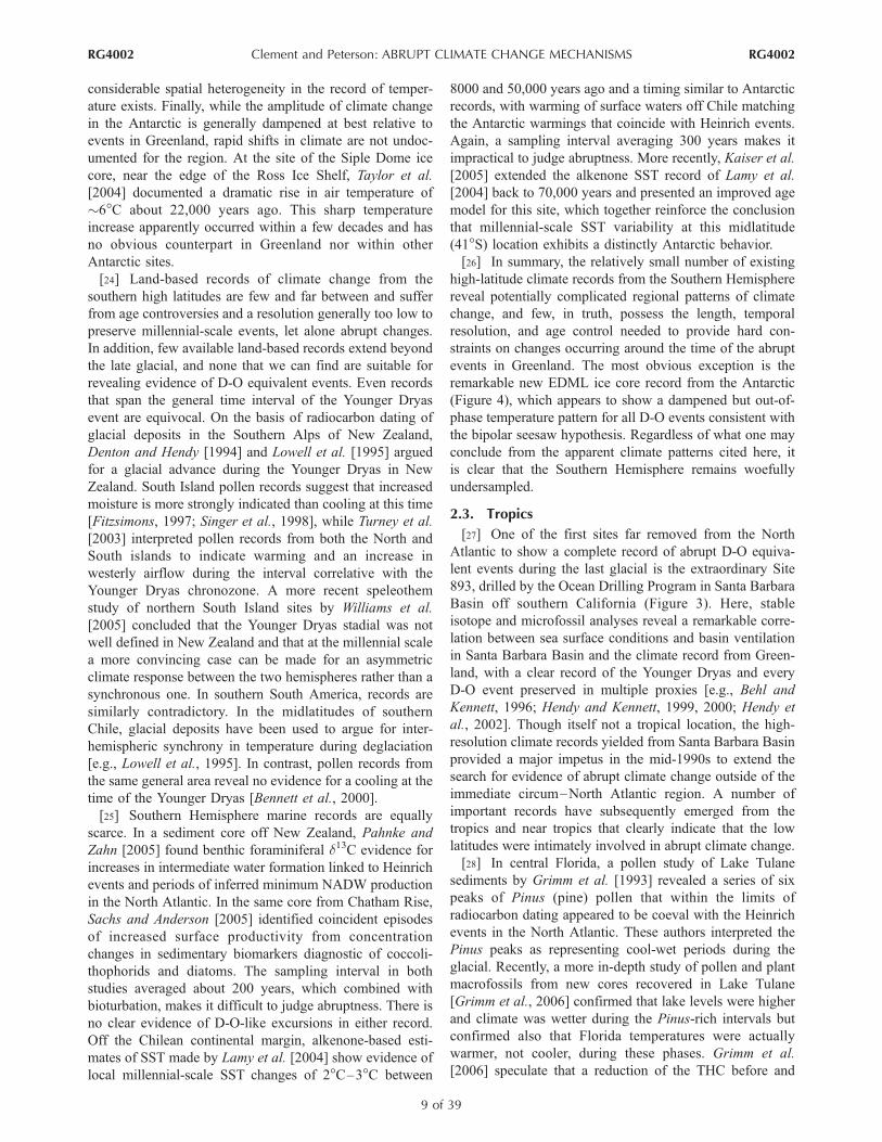
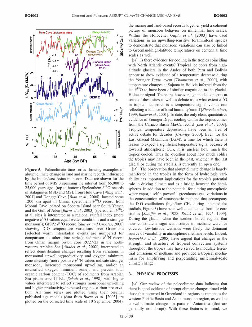
Figure 5. Paleoclimate time series showing examples ofabrupt climate change in land and marine records influencedby the Indian/east Asian monsoon. Data are shown for thetime period of MIS 3 spanning the interval from 65,000 to25,000 years ago. (top to bottom) Speleothem d18O recordsof stalagmites MSD and MSL from Hulu Cave [Wang et al.,2001] and Dongge Cave [Yuan et al., 2004], located some1200 km apart in China; speleothem d18O record fromMoomi Cave located on Socotra Island near South Yemenand the Gulf of Aden [Burns et al., 2003] (speleothem d18Oat all sites is interpreted as a regional rainfall index (morenegative d18O values equal wetter conditions and a strongermonsoon)); GISP2 d18O record [Stuiver and Grootes, 2000]showing D-O temperature variations over Greenland(selected warm interstadial events are numbered forcomparison to other time series); sediment d15N recordfrom Oman margin piston core RC27-23 in the north-western Arabian Sea [Altabet et al., 2002], interpreted toreflect denitrification changes resulting from variations inmonsoonal upwelling/productivity and oxygen minimumzone intensity (more positive d15N values indicate strongermonsoon, increased monsoonal upwelling, and/or anintensified oxygen minimum zone); and percent totalorganic carbon content (TOC) of sediments from ArabianSea piston core 111KL [Schulz et al., 1998], with highervalues interpreted to reflect stronger monsoonal upwellingand higher productivity/increased organic carbon preserva-tion. All time series are plotted using their originalpublished age models (data from Burns et al. [2003] areplotted on the corrected time scale of 10 September 2004).

RG4002 Clement and Peterson: ABRUPT CLIMATE CHANGE MECHANISMS

12 of 39

RG4002

now turn to physical mechanisms that can produce abrupt

changes and possibly link these remote regions. We proceed

by examining to what extent each mechanism can produce a

change that (1) is abrupt, (2) can persist and possibly recur

on millennial time scales, and (3) can link remote regions of

the globe.

3.1. Thermohaline Circulation

3.1.1. Abruptness[39] The first issue we address is whether the thermoha-

line circulation can change abruptly. The most common

explanation for an abrupt change in the THC is that it is

caused by a meltwater event. It is argued that if the fresh

meltwater flowing into the Atlantic reduces the salinity

sufficiently, then the waters will not be dense enough to

sink. Without the formation of deep water in the North

Atlantic, the balance of mass fluxes in the global ocean

between upwelling and diffusion will have to adjust, thereby

altering the thermohaline circulation globally [see Kuhlbrodt

et al., 2007]. The abruptness in this scenario can come about

in two ways. First, the meltwater event is generally por-

trayed as an abrupt perturbation to the system. At least two

different types of meltwater events have been suggested in

the literature. The first pertains to the Younger Dryas. For

that event, it has traditionally been argued that as the

Laurentide Ice Sheet melted back at the end of the last

glacial period, meltwaters flowing out of glacial Lake

Agassiz were diverted from a southern route through the

Mississippi drainage basin to the east and directly into the

North Atlantic. The second type of meltwater event pertains

to the Heinrich events. These events are defined by the

presence of layers of ice-rafted detritus in North Atlantic

sediments, indicating a significant source of fresh water

from melting icebergs. Hemming [2004] has suggested that

the provenance of these icebergs is the Hudson Strait, and

the surges are likely to have been caused by episodic

purging of the Laurentide Ice Sheet; however, other mech-

anisms are possible including jokulhlaup activity from

Hudson Bay lake or ice shelf buildup/collapse. Several

models of such behavior in glaciers have been constructed

(see Hemming [2004] for references); however, fully inter-

active, dynamic glacial ice has not been built into most

coupled climate models, so the connection between glacial

dynamics and ocean/atmosphere circulation has not yet

been tested.

[40] The second possible source of abruptness in the THC

behavior is the possibility that there are multiple stable

states of the THC. This was first suggested by Broecker et

al. [1985] and then demonstrated with a climate model by

Manabe and Stouffer [1988]. Since then, numerous ideal-

ized ocean-only and coupled models have been shown to

contain multiple stable states [Rahmstorf et al., 2005]. In

such models, minimal stochastic perturbations in freshwater

forcing can be sufficient to induce an abrupt change in

the THC strength [Ganopolski and Rahmstorf, 2001;

Timmermann et al., 2003]. It remains to be seen, however,

whether this behavior is an artifact of particular models

[e.g., Vellinga, 1998], whether it appears in more complete

models, or whether it is characteristic of the real climate

system. Experiments with the latest state-of-the art coupled

models do not appear to show such behavior. Stouffer et al.

[2006] conducted a coupled model intercomparison project

to test the response of a number of different models to a 0.1 Sv

addition of fresh water to the North Atlantic over 100 years,

after which the freshwater perturbation stops. The value of

0.1 Sv was chosen because it is comparable to the amount of

additional fresh water that models simulate will be added to

the North Atlantic because of large (i.e., 4 times the present)

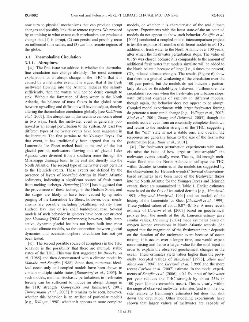
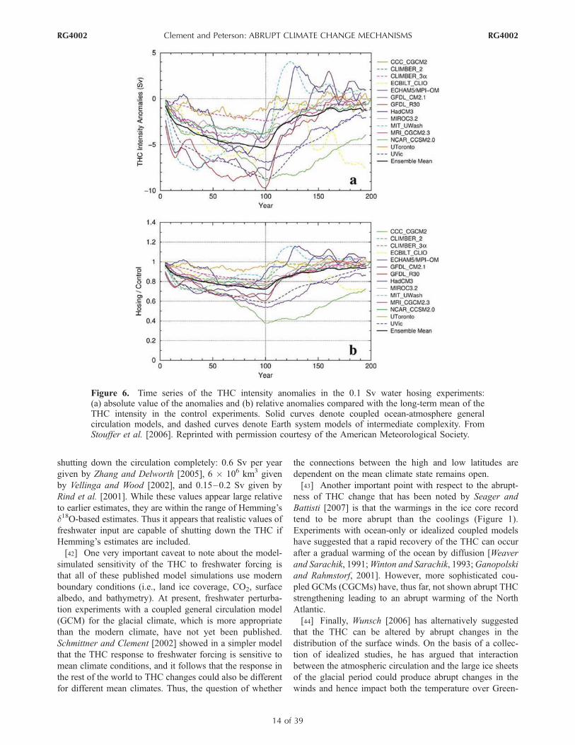
CO2-induced climate changes. The results (Figure 6) show

that there is a gradual weakening of the circulation over the

100 year period, but the models do not indicate a particu-

larly abrupt or threshold-type behavior. Furthermore, the

circulation recovers when the freshwater perturbation stops,

with different degrees of rapidity in different models,

though again, the behavior does not appear to be abrupt.

Coupled model experiments with larger freshwater forcing

do generate a more rapid change [e.g., Vellinga et al., 2002;

Rind et al., 2001; Zhang and Delworth, 2005], though the

models recover even from an essentially complete shutdown

and return to the modern strength of the THC, suggesting

that the ‘‘off’’ state is not a stable one, and overall, the

responses are generally linear to the size of the freshwater

perturbation [e.g., Rind et al., 2001].

[41] The freshwater perturbation experiments with mod-

els raise the issue of how large or ‘‘catastrophic’’ the

meltwater events actually were. That is, did enough melt-

water flood into the North Atlantic to collapse the THC

within decades to centuries in the models (as suggested by

the observations for Heinrich events)? Several observation-

based estimates have been made of the freshwater fluxes

into the North Atlantic for the Younger Dryas and Heinrich

events; these are summarized in Table 1. Earlier estimates

were based on the flux of ice-rafted detritus [e.g.,MacAyeal,

1993; Alley and MacAyeal, 1994] and on models of the

history of the Laurentide Ice Sheet [Licciardi et al., 1999].

These yielded values of about 0.07–0.1 Sv. A more recent

estimate of Carlson et al. [2007] based on geochemical

proxies from the mouth of the St. Laurence estuary gave

similar values. Hemming [2004] made estimates based on

oxygen isotope excursions in North Atlantic records. She

argued that the magnitude of the freshwater input depends

on the duration of the meltwater event because of ocean

mixing; if it occurs over a longer time, one would expect

more mixing and hence a larger value for the total input in

order to explain the observed geochemical changes in the

ocean. These estimates yield values higher than the previ-

ously accepted values of MacAyeal [1993], Alley and

MacAyeal [1994], and Licciardi et al. [1999] and the more

recent Carlson et al. [2007] estimate. In the model experi-

ments of Stouffer et al. [2006], a 0.1 Sv input of freshwater

per year reduces the THC strength by about 25% in

100 years (for the ensemble mean). This is clearly within

the range of observed meltwater estimates (and is on the low

side relative to Hemming’s estimates) but does not shut

down the circulation. Other modeling experiments have

shown that larger values of meltwater are capable of

RG4002 Clement and Peterson: ABRUPT CLIMATE CHANGE MECHANISMS

13 of 39

RG4002

shutting down the circulation completely: 0.6 Sv per year

given by Zhang and Delworth [2005], 6 � 106 km3 given

by Vellinga and Wood [2002], and 0.15–0.2 Sv given by

Rind et al. [2001]. While these values appear large relative

to earlier estimates, they are within the range of Hemming’s

d18O-based estimates. Thus it appears that realistic values of

freshwater input are capable of shutting down the THC if

Hemming’s estimates are included.

[42] One very important caveat to note about the model-

simulated sensitivity of the THC to freshwater forcing is

that all of these published model simulations use modern

boundary conditions (i.e., land ice coverage, CO2, surface

albedo, and bathymetry). At present, freshwater perturba-

tion experiments with a coupled general circulation model

(GCM) for the glacial climate, which is more appropriate

than the modern climate, have not yet been published.

Schmittner and Clement [2002] showed in a simpler model

that the THC response to freshwater forcing is sensitive to

mean climate conditions, and it follows that the response in

the rest of the world to THC changes could also be different

for different mean climates. Thus, the question of whether

the connections between the high and low latitudes are

dependent on the mean climate state remains open.

[43] Another important point with respect to the abrupt-

ness of THC change that has been noted by Seager and

Battisti [2007] is that the warmings in the ice core record

tend to be more abrupt than the coolings (Figure 1).

Experiments with ocean-only or idealized coupled models

have suggested that a rapid recovery of the THC can occur

after a gradual warming of the ocean by diffusion [Weaver

and Sarachik, 1991;Winton and Sarachik, 1993;Ganopolski

and Rahmstorf, 2001]. However, more sophisticated cou-

pled GCMs (CGCMs) have, thus far, not shown abrupt THC

strengthening leading to an abrupt warming of the North

Atlantic.

[44] Finally, Wunsch [2006] has alternatively suggested

that the THC can be altered by abrupt changes in the

distribution of the surface winds. On the basis of a collec-

tion of idealized studies, he has argued that interaction

between the atmospheric circulation and the large ice sheets

of the glacial period could produce abrupt changes in the

winds and hence impact both the temperature over Green-

Figure 6. Time series of the THC intensity anomalies in the 0.1 Sv water hosing experiments:(a) absolute value of the anomalies and (b) relative anomalies compared with the long-term mean of theTHC intensity in the control experiments. Solid curves denote coupled ocean-atmosphere generalcirculation models, and dashed curves denote Earth system models of intermediate complexity. FromStouffer et al. [2006]. Reprinted with permission courtesy of the American Meteorological Society.

RG4002 Clement and Peterson: ABRUPT CLIMATE CHANGE MECHANISMS

14 of 39

RG4002

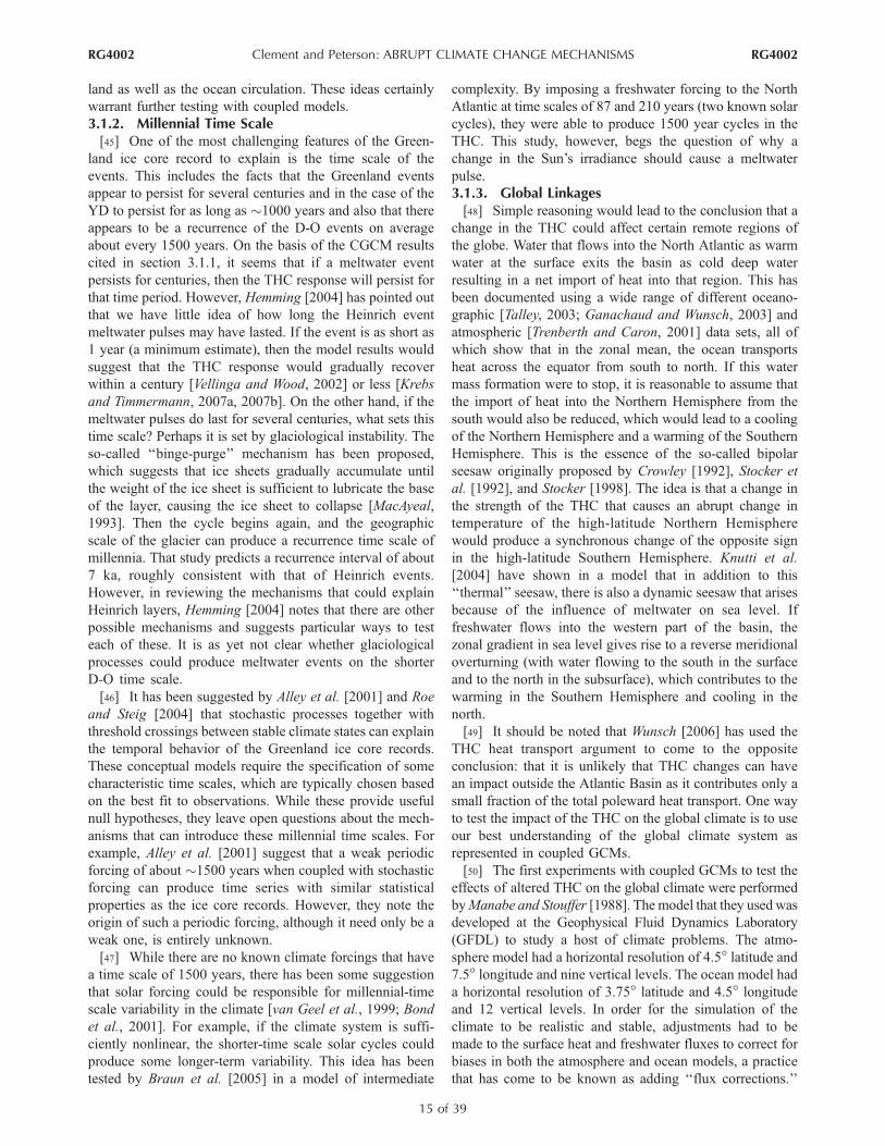
land as well as the ocean circulation. These ideas certainly

warrant further testing with coupled models.

3.1.2. Millennial Time Scale[45] One of the most challenging features of the Green-

land ice core record to explain is the time scale of the

events. This includes the facts that the Greenland events

appear to persist for several centuries and in the case of the

YD to persist for as long as �1000 years and also that there

appears to be a recurrence of the D-O events on average

about every 1500 years. On the basis of the CGCM results

cited in section 3.1.1, it seems that if a meltwater event

persists for centuries, then the THC response will persist for

that time period. However, Hemming [2004] has pointed out

that we have little idea of how long the Heinrich event

meltwater pulses may have lasted. If the event is as short as

1 year (a minimum estimate), then the model results would

suggest that the THC response would gradually recover

within a century [Vellinga and Wood, 2002] or less [Krebs

and Timmermann, 2007a, 2007b]. On the other hand, if the

meltwater pulses do last for several centuries, what sets this

time scale? Perhaps it is set by glaciological instability. The

so-called ‘‘binge-purge’’ mechanism has been proposed,

which suggests that ice sheets gradually accumulate until

the weight of the ice sheet is sufficient to lubricate the base

of the layer, causing the ice sheet to collapse [MacAyeal,

1993]. Then the cycle begins again, and the geographic

scale of the glacier can produce a recurrence time scale of

millennia. That study predicts a recurrence interval of about

7 ka, roughly consistent with that of Heinrich events.

However, in reviewing the mechanisms that could explain

Heinrich layers, Hemming [2004] notes that there are other

possible mechanisms and suggests particular ways to test

each of these. It is as yet not clear whether glaciological

processes could produce meltwater events on the shorter

D-O time scale.

[46] It has been suggested by Alley et al. [2001] and Roe

and Steig [2004] that stochastic processes together with

threshold crossings between stable climate states can explain

the temporal behavior of the Greenland ice core records.

These conceptual models require the specification of some

characteristic time scales, which are typically chosen based

on the best fit to observations. While these provide useful

null hypotheses, they leave open questions about the mech-

anisms that can introduce these millennial time scales. For

example, Alley et al. [2001] suggest that a weak periodic

forcing of about �1500 years when coupled with stochastic

forcing can produce time series with similar statistical

properties as the ice core records. However, they note the

origin of such a periodic forcing, although it need only be a

weak one, is entirely unknown.

[47] While there are no known climate forcings that have

a time scale of 1500 years, there has been some suggestion

that solar forcing could be responsible for millennial-time

scale variability in the climate [van Geel et al., 1999; Bond

et al., 2001]. For example, if the climate system is suffi-

ciently nonlinear, the shorter-time scale solar cycles could

produce some longer-term variability. This idea has been

tested by Braun et al. [2005] in a model of intermediate

complexity. By imposing a freshwater forcing to the North

Atlantic at time scales of 87 and 210 years (two known solar

cycles), they were able to produce 1500 year cycles in the

THC. This study, however, begs the question of why a

change in the Sun’s irradiance should cause a meltwater

pulse.

3.1.3. Global Linkages[48] Simple reasoning would lead to the conclusion that a

change in the THC could affect certain remote regions of

the globe. Water that flows into the North Atlantic as warm

water at the surface exits the basin as cold deep water

resulting in a net import of heat into that region. This has

been documented using a wide range of different oceano-

graphic [Talley, 2003; Ganachaud and Wunsch, 2003] and

atmospheric [Trenberth and Caron, 2001] data sets, all of

which show that in the zonal mean, the ocean transports

heat across the equator from south to north. If this water

mass formation were to stop, it is reasonable to assume that

the import of heat into the Northern Hemisphere from the

south would also be reduced, which would lead to a cooling

of the Northern Hemisphere and a warming of the Southern

Hemisphere. This is the essence of the so-called bipolar

seesaw originally proposed by Crowley [1992], Stocker et

al. [1992], and Stocker [1998]. The idea is that a change in

the strength of the THC that causes an abrupt change in

temperature of the high-latitude Northern Hemisphere

would produce a synchronous change of the opposite sign

in the high-latitude Southern Hemisphere. Knutti et al.

[2004] have shown in a model that in addition to this

‘‘thermal’’ seesaw, there is also a dynamic seesaw that arises

because of the influence of meltwater on sea level. If

freshwater flows into the western part of the basin, the

zonal gradient in sea level gives rise to a reverse meridional

overturning (with water flowing to the south in the surface

and to the north in the subsurface), which contributes to the

warming in the Southern Hemisphere and cooling in the

north.

[49] It should be noted that Wunsch [2006] has used the

THC heat transport argument to come to the opposite

conclusion: that it is unlikely that THC changes can have

an impact outside the Atlantic Basin as it contributes only a

small fraction of the total poleward heat transport. One way

to test the impact of the THC on the global climate is to use

our best understanding of the global climate system as

represented in coupled GCMs.

[50] The first experiments with coupled GCMs to test the

effects of altered THC on the global climate were performed

byManabe and Stouffer [1988]. The model that they used was

developed at the Geophysical Fluid Dynamics Laboratory

(GFDL) to study a host of climate problems. The atmo-

sphere model had a horizontal resolution of 4.5� latitude and7.5� longitude and nine vertical levels. The ocean model had

a horizontal resolution of 3.75� latitude and 4.5� longitudeand 12 vertical levels. In order for the simulation of the

climate to be realistic and stable, adjustments had to be

made to the surface heat and freshwater fluxes to correct for

biases in both the atmosphere and ocean models, a practice

that has come to be known as adding ‘‘flux corrections.’’

RG4002 Clement and Peterson: ABRUPT CLIMATE CHANGE MECHANISMS

15 of 39

RG4002

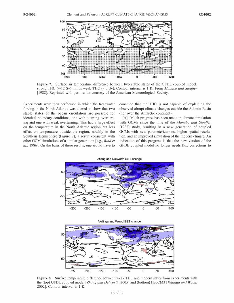
Experiments were then performed in which the freshwater

forcing in the North Atlantic was altered to show that two

stable states of the ocean circulation are possible for

identical boundary conditions, one with a strong overturn-

ing and one with weak overturning. This had a large effect

on the temperature in the North Atlantic region but less

effect on temperature outside the region, notably in the

Southern Hemisphere (Figure 7), a result consistent with

other GCM simulations of a similar generation [e.g., Rind et

al., 1986]. On the basis of these results, one would have to

conclude that the THC is not capable of explaining the

observed abrupt climate changes outside the Atlantic Basin

(nor over the Antarctic continent).

[51] Much progress has been made in climate simulation

with GCMs since the time of the Manabe and Stouffer

[1988] study, resulting in a new generation of coupled

GCMs with new parameterizations, higher spatial resolu-

tion, and an improved simulation of the modern climate. An

indication of this progress is that the new version of the

GFDL coupled model no longer needs flux corrections to

Figure 7. Surface air temperature difference between two stable states of the GFDL coupled model:strong THC (�12 Sv) minus weak THC (�0 Sv). Contour internal is 1 K. From Manabe and Stouffer[1988]. Reprinted with permission courtesy of the American Meteorological Society.

Figure 8. Surface temperature difference between weak THC and modern states from experiments withthe (top) GFDL coupled model [Zhang and Delworth, 2005] and (bottom) HadCM3 [Vellinga and Wood,2002]. Contour interval is 1 K.

RG4002 Clement and Peterson: ABRUPT CLIMATE CHANGE MECHANISMS

16 of 39

RG4002

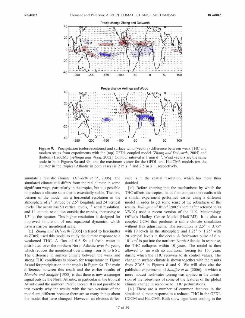
simulate a realistic climate [Delworth et al., 2006]. The

simulated climate still differs from the real climate in some

significant ways, particularly in the tropics, but it is possible

to produce a climate state that is essentially stable. The new

version of the model has a horizontal resolution in the

atmosphere of 2� latitude by 2.5� longitude and 24 vertical

levels. The ocean has 50 vertical levels, 1� zonal resolution,and 1� latitude resolution outside the tropics, increasing to

1/3� at the equator. This higher resolution is designed for

improved simulation of near-equatorial dynamics, which

have a narrow meridional scale.

[52] Zhang and Delworth [2005] (referred to hereinafter

as ZD05) used this model to study the climate response to a

weakened THC. A flux of 0.6 Sv of fresh water is

distributed over the northern North Atlantic over 60 years,

which reduces the meridional overturning from 16 to 6 Sv.

The difference in surface climate between the weak and

strong THC conditions is shown for temperature in Figure

8a and for precipitation in the tropics in Figure 9a. The main

difference between this result and the earlier results of

Manabe and Stouffer [1988] is that there is now a stronger

signal outside the North Atlantic, in particular in the tropical

Atlantic and the northern Pacific Ocean. It is not possible to

test exactly why the results with the two versions of the

model are different because there are so many things about

the model that have changed. However, an obvious differ-

ence is in the spatial resolution, which has more than

doubled.

[53] Before entering into the mechanisms by which the

THC affects the tropics, let us first compare the results with

a similar experiment performed earlier using a different

model in order to get some sense of the robustness of the

results. Vellinga and Wood [2002] (hereinafter referred to as

VW02) used a recent version of the U.K. Meteorology

Office’s Hadley Centre Model (HadCM3). It is also a

coupled GCM that produces a stable climate simulation

without flux adjustments. The resolution is 2.5� � 3.75�with 19 levels in the atmosphere and 1.25� � 1.25� with

20 vertical levels in the ocean. A freshwater pulse of 6 �105 km3 is put into the northern North Atlantic. In response,

the THC collapses within 10 years. The model is then

allowed to run with no additional forcing for 150 years

during which the THC recovers to its control values. The

change in surface climate is shown together with the results

from ZD05 in Figures 8 and 9. We will also cite the

published experiments of Stouffer et al. [2006], in which a

more modest freshwater forcing was applied in the discus-

sion of the robustness of some of the features of the global

climate change in response to THC perturbations.

[54] There are a number of common features in the

simulated climate response to a reduced THC in the GFDL

CGCM and HadCM3. Both show significant cooling in the

Figure 9. Precipitation (colors/contours) and surface wind (vectors) difference between weak THC andmodern states from experiments with the (top) GFDL coupled model [Zhang and Delworth, 2005] and(bottom) HadCM3 [Vellinga and Wood, 2002]. Contour interval is 1 mm d�1. Wind vectors are the samescale in both Figures 9a and 9b, and the maximum vector for the GFDL and HadCM3 models (on theequator in the tropical Atlantic in both cases) is 2 m s�1 and 2.5 m s�1, respectively.

RG4002 Clement and Peterson: ABRUPT CLIMATE CHANGE MECHANISMS

17 of 39

RG4002

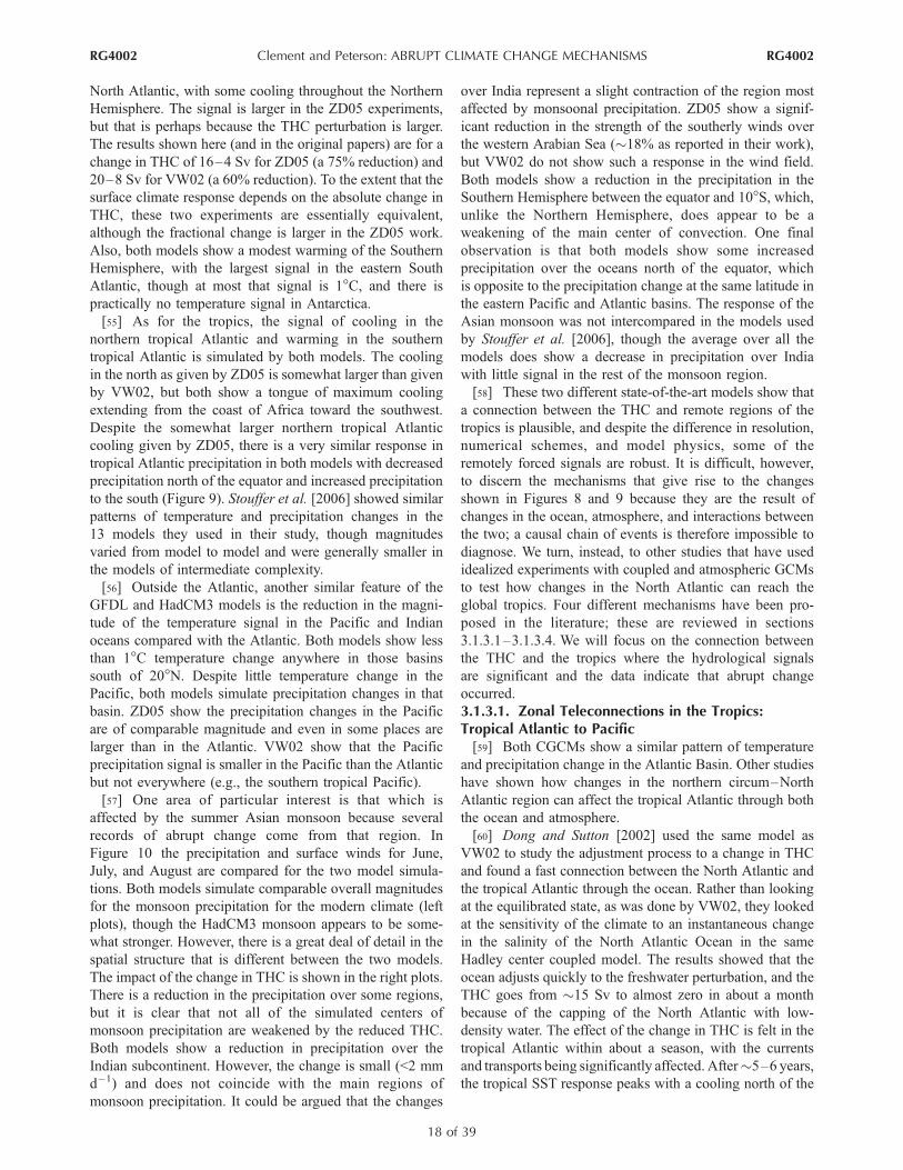
North Atlantic, with some cooling throughout the Northern

Hemisphere. The signal is larger in the ZD05 experiments,

but that is perhaps because the THC perturbation is larger.

The results shown here (and in the original papers) are for a

change in THC of 16–4 Sv for ZD05 (a 75% reduction) and

20–8 Sv for VW02 (a 60% reduction). To the extent that the

surface climate response depends on the absolute change in

THC, these two experiments are essentially equivalent,

although the fractional change is larger in the ZD05 work.

Also, both models show a modest warming of the Southern

Hemisphere, with the largest signal in the eastern South

Atlantic, though at most that signal is 1�C, and there is

practically no temperature signal in Antarctica.

[55] As for the tropics, the signal of cooling in the

northern tropical Atlantic and warming in the southern

tropical Atlantic is simulated by both models. The cooling

in the north as given by ZD05 is somewhat larger than given

by VW02, but both show a tongue of maximum cooling

extending from the coast of Africa toward the southwest.

Despite the somewhat larger northern tropical Atlantic

cooling given by ZD05, there is a very similar response in

tropical Atlantic precipitation in both models with decreased

precipitation north of the equator and increased precipitation

to the south (Figure 9). Stouffer et al. [2006] showed similar

patterns of temperature and precipitation changes in the

13 models they used in their study, though magnitudes

varied from model to model and were generally smaller in

the models of intermediate complexity.

[56] Outside the Atlantic, another similar feature of the

GFDL and HadCM3 models is the reduction in the magni-

tude of the temperature signal in the Pacific and Indian

oceans compared with the Atlantic. Both models show less

than 1�C temperature change anywhere in those basins

south of 20�N. Despite little temperature change in the

Pacific, both models simulate precipitation changes in that

basin. ZD05 show the precipitation changes in the Pacific

are of comparable magnitude and even in some places are

larger than in the Atlantic. VW02 show that the Pacific

precipitation signal is smaller in the Pacific than the Atlantic

but not everywhere (e.g., the southern tropical Pacific).

[57] One area of particular interest is that which is

affected by the summer Asian monsoon because several

records of abrupt change come from that region. In

Figure 10 the precipitation and surface winds for June,

July, and August are compared for the two model simula-

tions. Both models simulate comparable overall magnitudes

for the monsoon precipitation for the modern climate (left

plots), though the HadCM3 monsoon appears to be some-

what stronger. However, there is a great deal of detail in the

spatial structure that is different between the two models.

The impact of the change in THC is shown in the right plots.

There is a reduction in the precipitation over some regions,

but it is clear that not all of the simulated centers of

monsoon precipitation are weakened by the reduced THC.

Both models show a reduction in precipitation over the

Indian subcontinent. However, the change is small (<2 mm

d�1) and does not coincide with the main regions of

monsoon precipitation. It could be argued that the changes

over India represent a slight contraction of the region most

affected by monsoonal precipitation. ZD05 show a signif-

icant reduction in the strength of the southerly winds over

the western Arabian Sea (�18% as reported in their work),

but VW02 do not show such a response in the wind field.

Both models show a reduction in the precipitation in the

Southern Hemisphere between the equator and 10�S, which,unlike the Northern Hemisphere, does appear to be a

weakening of the main center of convection. One final

observation is that both models show some increased

precipitation over the oceans north of the equator, which

is opposite to the precipitation change at the same latitude in

the eastern Pacific and Atlantic basins. The response of the

Asian monsoon was not intercompared in the models used

by Stouffer et al. [2006], though the average over all the

models does show a decrease in precipitation over India

with little signal in the rest of the monsoon region.

[58] These two different state-of-the-art models show that

a connection between the THC and remote regions of the

tropics is plausible, and despite the difference in resolution,

numerical schemes, and model physics, some of the

remotely forced signals are robust. It is difficult, however,

to discern the mechanisms that give rise to the changes

shown in Figures 8 and 9 because they are the result of

changes in the ocean, atmosphere, and interactions between

the two; a causal chain of events is therefore impossible to

diagnose. We turn, instead, to other studies that have used

idealized experiments with coupled and atmospheric GCMs

to test how changes in the North Atlantic can reach the

global tropics. Four different mechanisms have been pro-

posed in the literature; these are reviewed in sections

3.1.3.1–3.1.3.4. We will focus on the connection between

the THC and the tropics where the hydrological signals

are significant and the data indicate that abrupt change

occurred.

3.1.3.1. Zonal Teleconnections in the Tropics:Tropical Atlantic to Pacific[59] Both CGCMs show a similar pattern of temperature

and precipitation change in the Atlantic Basin. Other studies

have shown how changes in the northern circum–North

Atlantic region can affect the tropical Atlantic through both

the ocean and atmosphere.

[60] Dong and Sutton [2002] used the same model as

VW02 to study the adjustment process to a change in THC

and found a fast connection between the North Atlantic and

the tropical Atlantic through the ocean. Rather than looking

at the equilibrated state, as was done by VW02, they looked

at the sensitivity of the climate to an instantaneous change

in the salinity of the North Atlantic Ocean in the same

Hadley center coupled model. The results showed that the

ocean adjusts quickly to the freshwater perturbation, and the

THC goes from �15 Sv to almost zero in about a month

because of the capping of the North Atlantic with low-

density water. The effect of the change in THC is felt in the

tropical Atlantic within about a season, with the currents

and transports being significantly affected. After�5–6 years,

the tropical SST response peaks with a cooling north of the

RG4002 Clement and Peterson: ABRUPT CLIMATE CHANGE MECHANISMS

18 of 39

RG4002

equator and a warming south of the equator, similar to the

pattern in Figure 8.

[61] Chiang et al. [2003] have argued that changes in the

northern circum–North Atlantic region influence the trop-

ical Atlantic through the atmosphere. They showed that

glacial boundary conditions, in particular ice sheets over

land, generate stronger trade winds and reduced SSTs in the

northern tropical Atlantic. The altered SST pattern shifts the

ITCZ to the south leading to significant precipitation

anomalies in the Atlantic Basin. Chiang et al. [2003] note

that such a pattern in meridional SST gradient and ITCZ

position is analogous to modern interannual climate vari-

ability [Moura and Shukla, 1981; Nobre and Shukla, 1996;

Chiang and Vimont, 2004]. Figure 9 shows that in both

coupled models, there is indeed an increase in the trade

winds in the northern tropical Atlantic and an anomalous

southerly flow across the equator, which are both consistent

with this ‘‘meridional mode’’ as well.

[62] In both models the tropical response to the THC is

not confined to the Atlantic. How does the signal get out of

the Atlantic and into the Pacific? Dong and Sutton [2002]

find that after 7 years, their perturbed experiments showed

an El Nino event developing in response to the freshening

of the North Atlantic. Those authors hypothesized that the

signal propagates from the tropical Atlantic into the Pacific

via atmospheric Rossby waves and then alters the surface

winds in the Pacific, initiating coupled feedbacks that lead

to an El Nino event. ZD05 invoke a similar pathway to

explain their results. They argue that the Pacific and

Atlantic are linked through the Central American region.

There is an increased sea level pressure (SLP) over the

northeastern tropical Pacific as a result of the Atlantic

changes; that is, the far northeastern ITCZ in the Pacific

appears to be strongly influenced by conditions in the

Atlantic, unlike the region just to the south that is strongly

influenced by the El Nino–Southern Oscillation (ENSO).

Figure 10. June, July, and August precipitation (colors/contours) and surface winds (vectors) from (top)Zhang and Delworth [2005] and (bottom) Vellinga and Wood [2002]. (left) Mean from the control runwith each model. Contour interval is 2 mm d�1, and maximum wind speed vector is 10 m s�1. (right)Difference between the weak THC and the control. Contour interval is 1 mm d�1. Wind vectors are thesame scale in all plots, and the maximum wind speed vector is 2 m s�1 for both models. The circles in theright plots show the locations of the paleoclimate records discussed in section 3.1.3. They are from Sinhaet al. [2005] for 30�N, 80�E; Stott et al. [2002] for 6�N, 125�E; Fleitmann et al. [2003] for 17�N, 54�E;Burns et al. [2003] for 12�N, 54�E; Wang et al. [2001] and Yuan et al. [2004] for 32�N, 119�E; andRosenthal et al. [2003] and Dannenmann et al. [2003] for 9�N, 122�E.

RG4002 Clement and Peterson: ABRUPT CLIMATE CHANGE MECHANISMS

19 of 39

RG4002

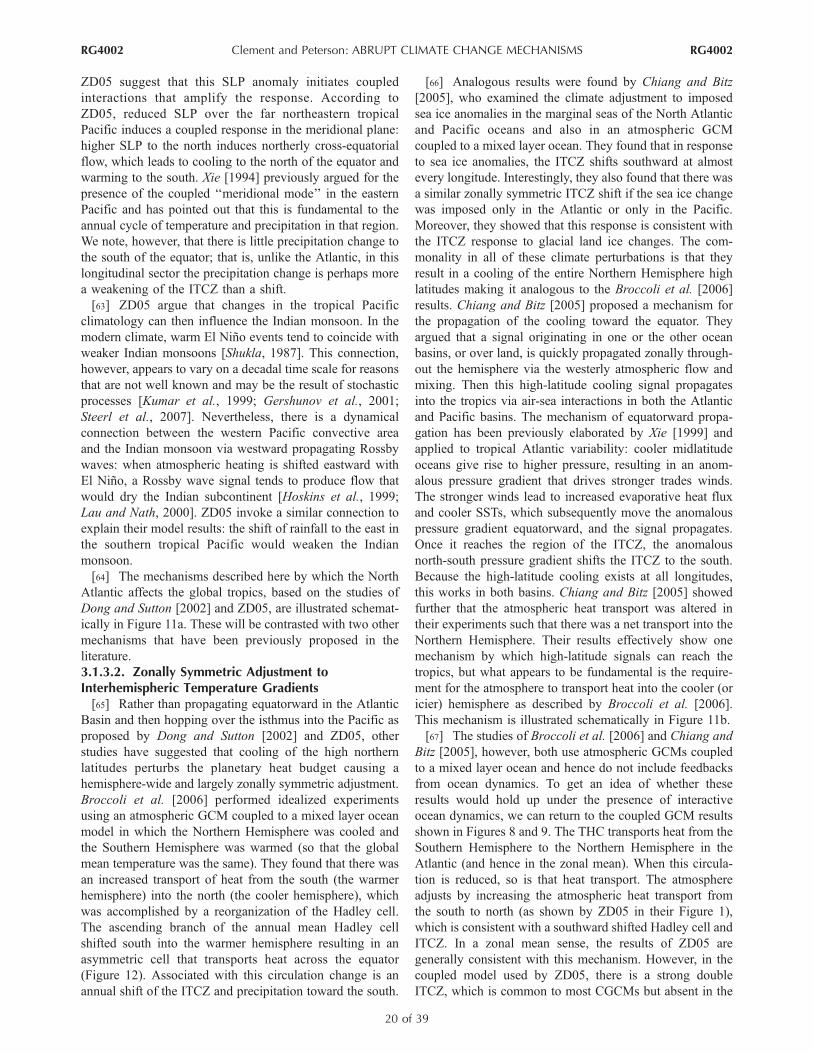
ZD05 suggest that this SLP anomaly initiates coupled

interactions that amplify the response. According to

ZD05, reduced SLP over the far northeastern tropical

Pacific induces a coupled response in the meridional plane:

higher SLP to the north induces northerly cross-equatorial

flow, which leads to cooling to the north of the equator and

warming to the south. Xie [1994] previously argued for the

presence of the coupled ‘‘meridional mode’’ in the eastern

Pacific and has pointed out that this is fundamental to the

annual cycle of temperature and precipitation in that region.

We note, however, that there is little precipitation change to

the south of the equator; that is, unlike the Atlantic, in this

longitudinal sector the precipitation change is perhaps more

a weakening of the ITCZ than a shift.

[63] ZD05 argue that changes in the tropical Pacific

climatology can then influence the Indian monsoon. In the

modern climate, warm El Nino events tend to coincide with

weaker Indian monsoons [Shukla, 1987]. This connection,

however, appears to vary on a decadal time scale for reasons

that are not well known and may be the result of stochastic

processes [Kumar et al., 1999; Gershunov et al., 2001;

Steerl et al., 2007]. Nevertheless, there is a dynamical

connection between the western Pacific convective area

and the Indian monsoon via westward propagating Rossby

waves: when atmospheric heating is shifted eastward with

El Nino, a Rossby wave signal tends to produce flow that

would dry the Indian subcontinent [Hoskins et al., 1999;

Lau and Nath, 2000]. ZD05 invoke a similar connection to

explain their model results: the shift of rainfall to the east in

the southern tropical Pacific would weaken the Indian

monsoon.

[64] The mechanisms described here by which the North

Atlantic affects the global tropics, based on the studies of

Dong and Sutton [2002] and ZD05, are illustrated schemat-

ically in Figure 11a. These will be contrasted with two other

mechanisms that have been previously proposed in the

literature.

3.1.3.2. Zonally Symmetric Adjustment toInterhemispheric Temperature Gradients[65] Rather than propagating equatorward in the Atlantic

Basin and then hopping over the isthmus into the Pacific as

proposed by Dong and Sutton [2002] and ZD05, other

studies have suggested that cooling of the high northern

latitudes perturbs the planetary heat budget causing a

hemisphere-wide and largely zonally symmetric adjustment.

Broccoli et al. [2006] performed idealized experiments

using an atmospheric GCM coupled to a mixed layer ocean

model in which the Northern Hemisphere was cooled and

the Southern Hemisphere was warmed (so that the global

mean temperature was the same). They found that there was

an increased transport of heat from the south (the warmer

hemisphere) into the north (the cooler hemisphere), which

was accomplished by a reorganization of the Hadley cell.

The ascending branch of the annual mean Hadley cell

shifted south into the warmer hemisphere resulting in an

asymmetric cell that transports heat across the equator

(Figure 12). Associated with this circulation change is an

annual shift of the ITCZ and precipitation toward the south.

[66] Analogous results were found by Chiang and Bitz

[2005], who examined the climate adjustment to imposed

sea ice anomalies in the marginal seas of the North Atlantic

and Pacific oceans and also in an atmospheric GCM

coupled to a mixed layer ocean. They found that in response

to sea ice anomalies, the ITCZ shifts southward at almost

every longitude. Interestingly, they also found that there was

a similar zonally symmetric ITCZ shift if the sea ice change

was imposed only in the Atlantic or only in the Pacific.

Moreover, they showed that this response is consistent with

the ITCZ response to glacial land ice changes. The com-

monality in all of these climate perturbations is that they

result in a cooling of the entire Northern Hemisphere high

latitudes making it analogous to the Broccoli et al. [2006]

results. Chiang and Bitz [2005] proposed a mechanism for

the propagation of the cooling toward the equator. They

argued that a signal originating in one or the other ocean

basins, or over land, is quickly propagated zonally through-

out the hemisphere via the westerly atmospheric flow and

mixing. Then this high-latitude cooling signal propagates

into the tropics via air-sea interactions in both the Atlantic

and Pacific basins. The mechanism of equatorward propa-

gation has been previously elaborated by Xie [1999] and

applied to tropical Atlantic variability: cooler midlatitude

oceans give rise to higher pressure, resulting in an anom-

alous pressure gradient that drives stronger trades winds.

The stronger winds lead to increased evaporative heat flux

and cooler SSTs, which subsequently move the anomalous

pressure gradient equatorward, and the signal propagates.

Once it reaches the region of the ITCZ, the anomalous

north-south pressure gradient shifts the ITCZ to the south.

Because the high-latitude cooling exists at all longitudes,

this works in both basins. Chiang and Bitz [2005] showed

further that the atmospheric heat transport was altered in

their experiments such that there was a net transport into the

Northern Hemisphere. Their results effectively show one

mechanism by which high-latitude signals can reach the

tropics, but what appears to be fundamental is the require-

ment for the atmosphere to transport heat into the cooler (or

icier) hemisphere as described by Broccoli et al. [2006].

This mechanism is illustrated schematically in Figure 11b.

[67] The studies of Broccoli et al. [2006] and Chiang and

Bitz [2005], however, both use atmospheric GCMs coupled

to a mixed layer ocean and hence do not include feedbacks

from ocean dynamics. To get an idea of whether these

results would hold up under the presence of interactive

ocean dynamics, we can return to the coupled GCM results

shown in Figures 8 and 9. The THC transports heat from the

Southern Hemisphere to the Northern Hemisphere in the

Atlantic (and hence in the zonal mean). When this circula-

tion is reduced, so is that heat transport. The atmosphere

adjusts by increasing the atmospheric heat transport from

the south to north (as shown by ZD05 in their Figure 1),

which is consistent with a southward shifted Hadley cell and

ITCZ. In a zonal mean sense, the results of ZD05 are

generally consistent with this mechanism. However, in the

coupled model used by ZD05, there is a strong double

ITCZ, which is common to most CGCMs but absent in the

RG4002 Clement and Peterson: ABRUPT CLIMATE CHANGE MECHANISMS

20 of 39

RG4002

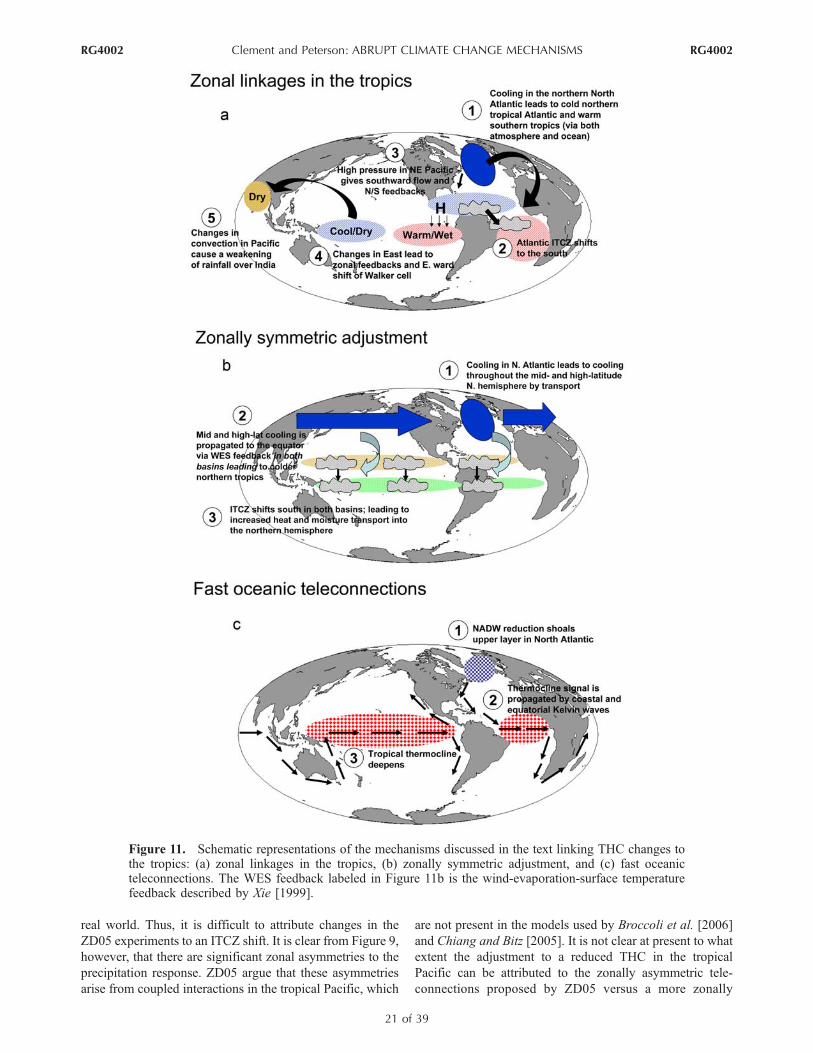
real world. Thus, it is difficult to attribute changes in the

ZD05 experiments to an ITCZ shift. It is clear from Figure 9,

however, that there are significant zonal asymmetries to the

precipitation response. ZD05 argue that these asymmetries

arise from coupled interactions in the tropical Pacific, which

are not present in the models used by Broccoli et al. [2006]

and Chiang and Bitz [2005]. It is not clear at present to what

extent the adjustment to a reduced THC in the tropical

Pacific can be attributed to the zonally asymmetric tele-

connections proposed by ZD05 versus a more zonally

Figure 11. Schematic representations of the mechanisms discussed in the text linking THC changes tothe tropics: (a) zonal linkages in the tropics, (b) zonally symmetric adjustment, and (c) fast oceanicteleconnections. The WES feedback labeled in Figure 11b is the wind-evaporation-surface temperaturefeedback described by Xie [1999].

RG4002 Clement and Peterson: ABRUPT CLIMATE CHANGE MECHANISMS

21 of 39

RG4002

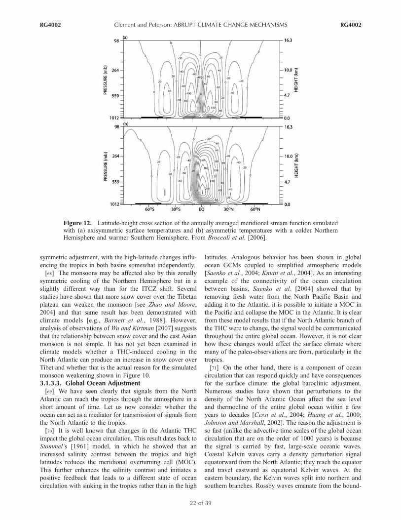
symmetric adjustment, with the high-latitude changes influ-

encing the tropics in both basins somewhat independently.

[68] The monsoons may be affected also by this zonally

symmetric cooling of the Northern Hemisphere but in a

slightly different way than for the ITCZ shift. Several

studies have shown that more snow cover over the Tibetan

plateau can weaken the monsoon [see Zhao and Moore,

2004] and that same result has been demonstrated with

climate models [e.g., Barnett et al., 1988]. However,

analysis of observations ofWu and Kirtman [2007] suggests

that the relationship between snow cover and the east Asian

monsoon is not simple. It has not yet been examined in

climate models whether a THC-induced cooling in the

North Atlantic can produce an increase in snow cover over

Tibet and whether that is the actual reason for the simulated

monsoon weakening shown in Figure 10.

3.1.3.3. Global Ocean Adjustment[69] We have seen clearly that signals from the North

Atlantic can reach the tropics through the atmosphere in a

short amount of time. Let us now consider whether the

ocean can act as a mediator for transmission of signals from

the North Atlantic to the tropics.

[70] It is well known that changes in the Atlantic THC

impact the global ocean circulation. This result dates back to

Stommel’s [1961] model, in which he showed that an

increased salinity contrast between the tropics and high

latitudes reduces the meridional overturning cell (MOC).

This further enhances the salinity contrast and initiates a

positive feedback that leads to a different state of ocean

circulation with sinking in the tropics rather than in the high

latitudes. Analogous behavior has been shown in global

ocean GCMs coupled to simplified atmospheric models

[Saenko et al., 2004; Knutti et al., 2004]. As an interesting

example of the connectivity of the ocean circulation

between basins, Saenko et al. [2004] showed that by

removing fresh water from the North Pacific Basin and

adding it to the Atlantic, it is possible to initiate a MOC in

the Pacific and collapse the MOC in the Atlantic. It is clear

from these model results that if the North Atlantic branch of

the THC were to change, the signal would be communicated

throughout the entire global ocean. However, it is not clear

how these changes would affect the surface climate where

many of the paleo-observations are from, particularly in the

tropics.

[71] On the other hand, there is a component of ocean

circulation that can respond quickly and have consequences

for the surface climate: the global baroclinic adjustment.

Numerous studies have shown that perturbations to the

density of the North Atlantic Ocean affect the sea level

and thermocline of the entire global ocean within a few

years to decades [Cessi et al., 2004; Huang et al., 2000;

Johnson and Marshall, 2002]. The reason the adjustment is

so fast (unlike the advective time scales of the global ocean

circulation that are on the order of 1000 years) is because

the signal is carried by fast, large-scale oceanic waves.

Coastal Kelvin waves carry a density perturbation signal

equatorward from the North Atlantic; they reach the equator

and travel eastward as equatorial Kelvin waves. At the

eastern boundary, the Kelvin waves split into northern and

southern branches. Rossby waves emanate from the bound-

Figure 12. Latitude-height cross section of the annually averaged meridional stream function simulatedwith (a) axisymmetric surface temperatures and (b) asymmetric temperatures with a colder NorthernHemisphere and warmer Southern Hemisphere. From Broccoli et al. [2006].

RG4002 Clement and Peterson: ABRUPT CLIMATE CHANGE MECHANISMS

22 of 39

RG4002

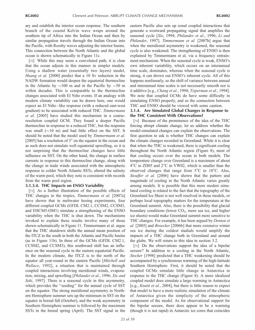
ary and establish the interior ocean response. The southern

branch of the coastal Kelvin wave wraps around the

southern tip of Africa into the Indian Ocean and then by

similar propagation travels through the Indian Ocean into

the Pacific, with Rossby waves adjusting the interior basins.

This connection between the North Atlantic and the global

ocean is shown schematically in Figure 11c.

[72] While this may seem a convoluted path, it is clear

that the ocean adjusts in this manner in simpler models.

Using a shallow water (essentially two layers) model,

Huang et al. [2000] predict that a 10 Sv reduction in the

NADW formation would deepen the equatorial thermocline

in the Atlantic by �100 m and in the Pacific by �50 m

within decades. This is comparable to the thermocline

changes associated with El Nino events. If an analogy with

modern climate variability can be drawn here, one would

expect an El Nino–like response (with a reduced east-west

gradient) to be associated with reduced THC. Timmermann

et al. [2005] have studied this mechanism in a coarse-

resolution coupled GCM. They found a deeper Pacific

thermocline in response to a reduced THC, but the response

was small (�10 m) and had little effect on the SST. It

should be noted that the model used by Timmermann et al.

[2005] has a resolution of 3� on the equator in the ocean andas such does not simulate well equatorial upwelling, so it is

not surprising that the thermocline changes have little

influence on SST. On the other hand, the change in surface

currents in response to this thermocline change, along with

the change in trade winds associated with the atmospheric

response to colder North Atlantic SSTs, altered the salinity

of the warm pool, which they note is consistent with records

from the warm pool region.

3.1.3.4. THC Impacts on ENSO Variability[73] As a further illustration of the possible effects of

THC changes in the tropics, Timmermann et al. [2007a]

have shown that in meltwater hosing experiments, four

different coupled GCMs (GFDL CM2.1, CCSM2, CCSM3,

and EHCM5-OM1) simulate a strengthening of the ENSO

variability when the THC is shut down. The mechanisms

invoked to explain these results involve many of those

shown schematically in Figure 11. Timmermann et al. argue

that the THC shutdown shifts the annual mean position of

the ITCZ to the south in both the Atlantic and Pacific basins

(as in Figure 11b). In three of the GCMs (GFDL CM2.1,

CCSM2, and CCSM3), this southward shift has an influ-

ence on the seasonal cycle in the eastern equatorial Pacific.

In the modern climate, the ITCZ is to the north of the

equator all year-round in the eastern Pacific [Mitchell and

Wallace, 1992], a situation that is maintained through

coupled interactions involving meridional winds, evapora-

tion, mixing, and upwelling [Philander et al., 1996; Xie and

Seki, 1997]. There is a seasonal cycle in this asymmetry,

which provides the ‘‘seeding’’ for the annual cycle of SST

on the equator. The strong meridional asymmetry in North-

ern Hemisphere summer sets up the minimum in SST on the

equator in boreal fall (October), and the weak asymmetry in

Southern Hemisphere summer is followed by the maximum

SSTs in the boreal spring (April). The SST signal in the

eastern Pacific also sets up zonal coupled interactions that

generate a westward propagating signal that amplifies the

seasonal cycle [Xie, 1994; Philander et al., 1996; Li and

Philander, 1997]. Timmermann et al. [2007b] argue that

when the meridional asymmetry is weakened, the seasonal

cycle is also weakened. The strengthening of ENSO is then

explained by Timmermann et al. via a frequency entrain-

ment mechanism. When the seasonal cycle is weak, ENSO’s

own inherent variability, which occurs on an interannual

time scale, dominates, whereas when the seasonal cycle is

strong, it can drown out ENSO’s inherent cycle. All of this

happens nonlinearly, so the shift of variance between annual

and interannual time scales is not necessarily smooth nor is

it additive [e.g., Chang et al., 1994; Tziperman et al., 1994].

We note that coupled GCMs do have some difficulty in

simulating ENSO properly, and so the connection between

THC and ENSO should be viewed with some caution.

3.1.4. Are Simulated Global Changes in Response tothe THC Consistent With Observations?[74] Because of the prominence of the idea of the THC

forcing abrupt climate change, let us address whether the

model-simulated changes can explain the observations. The

first question to ask is whether THC changes can explain

the climate changes recorded in Greenland. While it is clear

that when the THC is weakened, there is significant cooling

throughout the North Atlantic region (Figure 8), most of

that cooling occurs over the ocean in both models. The

temperature change over Greenland is a maximum of about

4�C in ZD05 and 2�C in VW02, which is smaller than the

observed changes that range from 5�C to 10�C. Also,

Stouffer et al. [2006] have shown that the pattern and

magnitude of cooling in the North Atlantic varies greatly

among models. It is possible that this more modest simu-

lated cooling is related to the fact that the topography of the

Greenland Ice Sheet is not well resolved in these models, or

perhaps local topography matters for the temperature at the

Greenland summit. Also, there is the possibility that glacial

boundary conditions (lower CO2, more sea ice, and higher

ice sheets) would make Greenland summit more sensitive to

THC changes. For example, it has been argued by Denton et

al. [2005] and Broecker [2006b] that more extensive winter

sea ice during the coldest stadials would amplify the

impacts of a THC change both in Greenland and around

the globe. We will return to this idea in section 3.2.

[75] Do the observations support the idea of a bipolar

seesaw? In addition to a cooling in the North Atlantic,

Stocker [1998] predicted that a THC weakening should be

accompanied by a synchronous warming of the high-latitude

Southern Hemisphere. First, it should be noted that the

coupled GCMs simulate little change in Antarctica in

response to the THC change (Figure 8). A more idealized

coupled model does simulate a large warming in Antarctica

[e.g., Knutti et al., 2004], but there is little reason to expect

that model to have a more realistic simulation of the climate

of Antarctica given the simplicity of the atmospheric

component of the model. As for observational support for

the bipolar seesaw, there does appear to be a warming

(though it is not rapid) in Antarctic ice cores that coincides

RG4002 Clement and Peterson: ABRUPT CLIMATE CHANGE MECHANISMS

23 of 39

RG4002

with Heinrich events, which can be explained as an inte-

grated response to the changes in the North Atlantic [Roe

and Steig, 2004]. The EPICA core also shows the D-O

events [EPICA Community Members, 2006], and the EPICA

Community Members claim that the magnitude of the

warming in Antarctica is proportional to the duration of

the THC change in the North Atlantic. It should be noted,

however, that the Antarctic record was compared with the

GRIP record, not a proxy for THC variations, which are

presently equivocal for D-O events.

[76] For the tropics, we will focus here on the distinction

between the temperature and hydrologic signatures of the

THC response in the tropics. As discussed in section 3.1.3,

the models show a temperature change in the tropical

Atlantic Basin, with little change outside. A cooling in the

subtropical North Atlantic has been observed by Sachs and

Lehman [1999] and Bard et al. [2000]; however the cooling

predicted by those studies is larger than that simulated by

the model, as pointed out by Seager and Battisti [2007]. The

3�C–4�C temperature change in Cariaco Basin is also larger

than the model-simulated cooling, although local changes in

upwelling that may not be well simulated by the model

could potentially enhance the coastal signal. The absence of

a large cooling associated with the Greenland events in

other parts of the tropics may simply be due to a lack of

reliable records. However, at this point the available obser-

vations appear to be consistent with the model in that the

only clear signal of cooling is in the North Atlantic.

[77] The precipitation patterns in the tropical Atlantic

Basin have been quite convincingly linked to THC-driven

shifts in the ITCZ [Peterson and Haug, 2006; Seager and

Battisti, 2007]. However, as one moves outside the tropical

Atlantic, the consistency between models and observations

becomes less compelling. The models simulate a robust

increase in precipitation in the southern central Pacific, but

there are no data available from that region. Both models

simulate changes in precipitation in the western Pacific

warm pool during boreal summer, but the pattern is not

consistent. The record of Stott et al. [2002] and the Sulu Sea

records both indicate saltier waters during stadials, which

are consistent with the GFDL model decrease in precipita-

tion, but the model signal is quite small (on the order of

10%). However, local salinity (which is how the Stott et al.

record is interpreted) is not determined only by local

precipitation, as illustrated by Timmermann et al. [2005].

Without a more complete analysis of the model results, it is

difficult to link salinity changes at this site with large-scale

THC-induced changes. Both models predict a weakening of

Indian rainfall, which appears to be consistent with Sinha et

al. [2005], though this record only covers the Bølling-Allerød

(15.2–11.7 ka). Neither model predicts much precipitation

change over Southeast Asia where the speleothem records

of Wang et al. [2001] and Yuan et al. [2004] are from, nor

do they predict much change over Oman as do Fleitmann et

al. [2003] or Socotra Island as do Burns et al. [2003]. The

GFDL model does simulate a significant change in the

southwesterly surface winds, which would be consistent

with the change in productivity records from the Arabian

Sea [Schulz et al., 1998; Altabet et al., 2002; Gupta et al.,

2003], but this does not appear in HadCM3. Thus it seems

that the real-world events are more widespread in their

monsoon response than the models simulate.

3.2. Sea Ice

[78] Several papers have suggested that a potential driver

for abrupt climate change is sea ice. Sea ice has two

different and strong influences on climate. The first is

through its albedo, which can alter both the local and the

global energy budget [North, 1984], and the second is

through insulating the ocean from the atmosphere by cutting

off the exchange of heat and moisture, thereby having a

strong influence on the local climate. Here we review the

studies suggesting sea ice as an important mechanism in

abrupt change, again with attention to whether they can

explain climate events that are abrupt, persistent/recurrent

on millennial time scales, and have a global influence.

3.2.1. Abruptness[79] The key to the possible abrupt behavior of sea ice is

that (1) there is a temperature threshold for its formation and

melt and (2) sea ice can melt and advance rapidly because of

albedo feedback. Gildor and Tziperman [2001, 2003]

further argued that there is another possible sea ice

‘‘switch,’’ which is that as sea ice grows, the ability of the

ocean to lose heat to the atmosphere is cut off, and at some

point it cannot cool sufficiently, so it stops growing. Hence,

Gildor and Tziperman argue that sea ice has both ‘‘on’’ and

‘‘off’’ switches. As such, it has been argued that sea ice can

respond abruptly to changes in THC or atmospheric circu-

lation and amplify the perturbation both locally and perhaps

globally.

[80] Kaspi et al. [2004] used a box model to demonstrate

how ice sheet dynamics, ocean, atmosphere, and sea ice can

interact to produce Heinrich-like events. There are three

phases of the oscillation that represent different states of

North Atlantic sea ice cover; they are shown in Figure 13.

Following a meltwater event (which in their formulation is

caused by the ‘‘purge’’ phase of an ice sheet), the THC

reduces and hence sea ice extends farther equatorward with

a large reduction in high-latitude temperatures. Once the

meltwater event ends, the THC begins to recover and melt

back the sea ice, but the albedo and insulating effects of the

reduction in sea ice amplify this, causing widespread

melting and ultimately resulting in a minimum sea ice state.

With sea ice extent at a minimum, the ocean temperature

begins to cool because of heat loss to the atmosphere, which

eventually leads to a readvance of the sea ice back to its

initial levels. While highly simplified, this model nicely

illustrates some of the key interactions between the ice sheets,

ocean, atmosphere, and sea ice.Gildor and Tziperman [2001]

used a similar model to argue that self-sustained oscillations

involving these feedbacks can arise on 100 ka time scale

and also reproduce the asymmetric, ‘‘sawtooth’’ pattern in

glacial cycles. They did not find, however, that such

oscillations would arise on millennial time scales. Thus,

sea ice plays a key role in generating the abrupt swings as

RG4002 Clement and Peterson: ABRUPT CLIMATE CHANGE MECHANISMS

24 of 39

RG4002

the system adjusts itself back to an initial state, but the land-

based ice sheets are required as a ‘‘trigger.’’

[81] Do these feedback mechanisms play out in more

complete models? There is little discussion of sea ice

feedback in the freshwater hosing studies cited earlier

(VW02, ZD05, and Stouffer et al. [2006]). It seems likely

that changes in sea ice are responsible for some of the large

temperature changes (up to 10�C) over the North Atlantic

Ocean (shown in Figure 8), though Stouffer et al. [2006]

show that the pattern and magnitude of cooling (and

perhaps sea ice) in the North Atlantic varies greatly among

models. The issue of the quantitative relationship between

THC and sea ice and its subsequent effects on regional

climate appears to be an area ripe for exploration.

[82] The issue of rapid sea ice change has received

considerable attention of late because of the possible effect

of present and future increases in CO2 on Arctic ice cover

[Vinnikov et al., 1999; Stroeve et al., 2007]. Winton [2006]

has explored the behavior of sea ice feedbacks in coupled

models under increasing CO2 and found that in two models

(Max Planck Institute and National Center for Atmospheric

Research (NCAR)), sea ice disappeared year round. He

found that the ice-albedo feedback as demonstrated in

simpler models [North, 1984] was responsible for rapid

changes in sea ice. Thus, it does appear that this feedback is

plausible, though further study is necessary to understand

how sea ice behaves in these models, not to mention in the

real climate system.

3.2.2. Millennial Time Scale[83] Sea ice mechanisms do not in themselves introduce

any millennial time scale behavior into the system, because

the adjustment time scale is relatively short (as illustrated in

Figure 13). It is possible that sea ice interacts with the ice

sheets to introduce longer-term oscillations. Gildor and

Tziperman [2001] have argued for this on a 100 ka time

scale but not on millennial time scales. Aside from that, the

only likely form of millennial recurrence comes from glacial

dynamics with sea ice acting as a potential amplifier.

3.2.3. Global Linkages[84] Li et al. [2005] argued on the basis of atmospheric

modeling experiments that the large magnitude of warming

during D-O events in Greenland can be explained by a

removal of sea ice in the North Atlantic. They performed

experiments with the NCAR CCM3 model with glacial

boundary conditions (CO2, ice sheets, SST, and sea ice)

and then changed the sea ice to its modern extent, leaving

all other glacial boundary conditions the same. Li et al. find

that a reduction in winter sea ice, through both its albedo

and insulation effects, can explain the magnitude of tem-

perature and accumulation changes over Greenland during

D-O warmings. Denton et al. [2005] argue further that

wintertime sea ice is necessary to explain not only changes

in ice core records from Greenland summit but also the

pattern of moraines from the whole circum–North Atlantic

region. A wintertime sea ice advance in the North Atlantic

(e.g., as hypothesized for the YD) would make winters

much colder throughout the region and hence would explain

the significant seasonality shown in proxies from around the

region.

[85] We have already discussed the study of Chiang and

Bitz [2005] that showed that changes in sea ice anywhere in

the Northern Hemisphere high latitudes could produce a

climate change throughout the tropics. Their mechanism is

illustrated in Figure 11b.

3.3. Tropical Ocean-Atmosphere Processes

3.3.1. Abruptness[86] There is some evidence from the modern climate that

the tropics are capable of undergoing abrupt change. A shift

in surface temperatures in the tropical Pacific occurred in

Figure 13. Three sea ice state mechanisms for the Heinrich cycle in a coupled model with a continuousmeridional resolution. Periodic freshwater (glacier) discharge is specified in this model, and the responseof the ocean, sea ice, and atmosphere is calculated and shown here. A detailed model description isprovided by Kaspi et al. [2004, Appendix A]. This model experiment demonstrates that the triple sea icestate response to glacier discharges, which occurs in a simpler box model, also occurs in this fullercontinuous model. Model time series for (a) the specified freshwater (glacial discharge) input into thenorthern region of the ocean model, (b) the maximum THC in the Northern Hemisphere, (c) sea ice extentin the Northern Hemisphere (latitude of the southernmost point covered with sea ice), and (d) averagedatmospheric temperature from 30�N to 70�N showing the atmospheric response to sea ice switches. Thecold periods are highlighted by gray bands. From Kaspi et al. [2004].

RG4002 Clement and Peterson: ABRUPT CLIMATE CHANGE MECHANISMS

25 of 39

RG4002

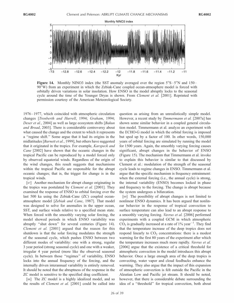
1976–1977, which coincided with atmospheric circulation

changes [Trenberth and Hurrell, 1994; Graham, 1994;

Deser et al., 2004] as well as large ecosystem shifts [Bakun

and Broad, 2003]. There is considerable controversy about

what caused the change and the extent to which it represents

a ‘‘regime shift.’’ Some argue that it had its origins in the

midlatitudes [Barnett et al., 1999], but others have suggested

that it originated in the tropics. For example, Karspeck and

Cane [2002] have shown that the oceanic changes in the

tropical Pacific can be reproduced by a model forced only

by observed equatorial winds. Regardless of the origin of

the wind changes, this result suggests that mechanisms

within the tropical Pacific are responsible for the abrupt

oceanic changes; that is, the trigger for change is in the

tropical winds.

[87] Another mechanism for abrupt change originating in

the tropics was postulated by Clement et al. [2001]. They

examined the response of ENSO to orbital forcing over the

last 500 ka using the Zebiak-Cane (ZC) coupled ocean-

atmosphere model [Zebiak and Cane, 1987]. That model

was designed to solve for anomalies in the upper ocean,

SST, and surface winds relative to a specified mean state.

When forced with the smoothly varying solar forcing, the

model showed periods in which ENSO variability was

abruptly ‘‘shut down’’ for several centuries (Figure 14).

Clement et al. [2001] argued that the reason for this

shutdown is that the solar forcing modulates the strength

of the seasonal cycle, which pushes ENSO between two

different modes of variability: one with a strong, regular

3 year period (strong seasonal cycle) and one with a weaker,

irregular 4 year period (more like the observed seasonal

cycle). In between those ‘‘regimes’’ of variability, ENSO

locks into the annual frequency of the forcing, and the

internally driven interannual variability is entirely removed.

It should be noted that the abruptness of the response in the

ZC model is sensitive to the specified drag coefficient.

[88] The ZC model is a highly idealized model, and so

the results of Clement et al. [2001] could be called into

question as arising from an unrealistically simple model.

However, a recent study by Timmermann et al. [2007a] has

shown some similar behavior in a coupled general circula-

tion model. Timmermann et al. analyze an experiment with

the ECHO-G model in which the orbital forcing is imposed

but sped up by a factor of 100. In other words, 150,000

years of orbital forcing are simulated by running the model

for 1500 years. Again, the smoothly varying forcing causes

significant, abrupt changes in the behavior of ENSO

(Figure 15). The mechanism that Timmermann et al. invoke

to explain this behavior is similar to that discussed by

Clement et al.: modulation of the strength of the seasonal

cycle leads to regime changes in ENSO. Timmermann et al.

argue that the specific mechanism is frequency entrainment:

when the external forcing (i.e., the annual cycle) is strong,

the internal variability (ENSO) becomes locked in phase

and frequency to the forcing. The change is abrupt because

the system undergoes a bifurcation.

[89] The possibility of abrupt changes is not limited to

nonlinear ENSO dynamics. It has been argued that nonlin-

ear behavior in the response of tropical convection to

surface temperature can also lead to an abrupt response to

a smoothly varying forcing. Vavrus et al. [2006] performed

experiments with a coupled GCM in which atmospheric

CO2 is gradually increased at a rate of 1% year�1. They find

that the temperature increase of the deep tropics does not

respond linearly to CO2 concentrations: there is a modest

warming for the first 80 years of the experiment after which

the temperature increases much more rapidly. Vavrus et al.

[2006] argue that the existence of a critical threshold for

atmospheric convection in the model introduces this abrupt

behavior. Once a large enough area of the deep tropics is

convecting, water vapor and cloud feedbacks enhance the

warming. They also argue that the impact of this expansion

of atmospheric convection is felt outside the Pacific in the

Aleutian Low and Pacific jet stream. It should be noted,

however, that there is considerable debate surrounding the

idea of a ‘‘threshold’’ for tropical convection, both about

Figure 14. Monthly NINO3 index (the SST anomaly averaged over the region 5�S–5�N and 150–90�W) from an experiment in which the Zebiak-Cane coupled ocean-atmosphere model is forced withorbitally driven variations in solar insolation. How ENSO in the model abruptly locks to the seasonalcycle around the time of the Younger Dryas is shown. From Clement et al. [2001]. Reprinted withpermission courtesy of the American Meteorological Society.

RG4002 Clement and Peterson: ABRUPT CLIMATE CHANGE MECHANISMS

26 of 39

RG4002

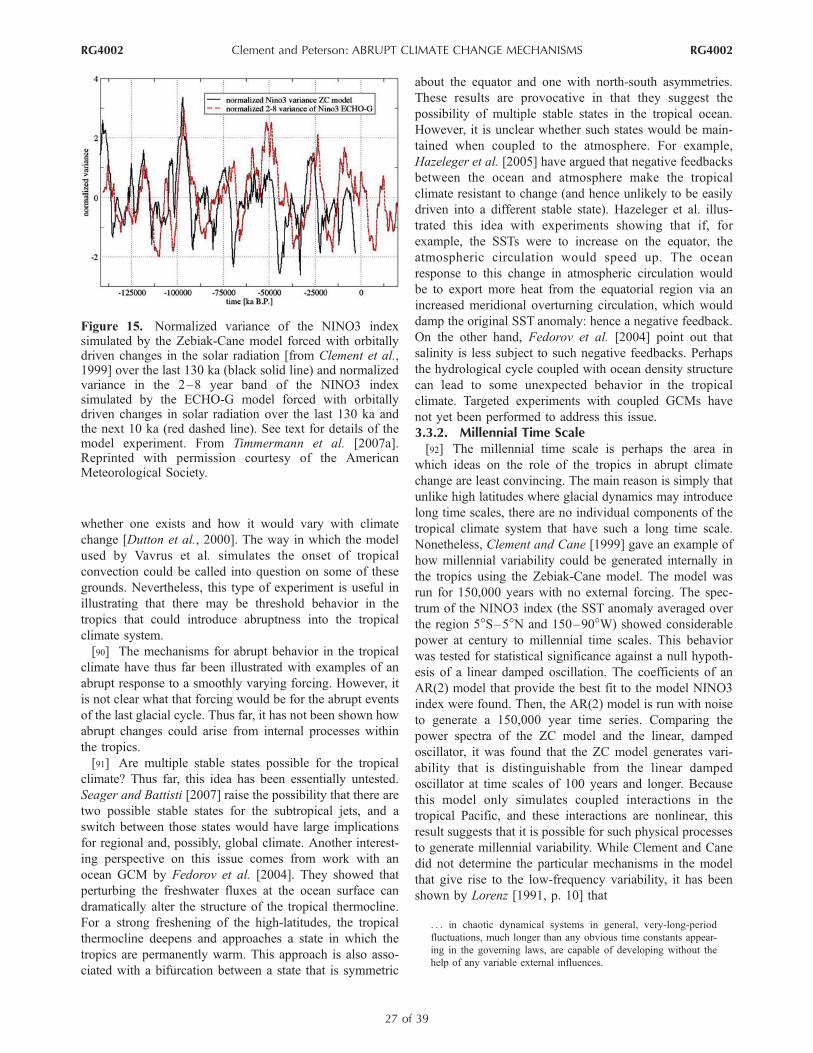
whether one exists and how it would vary with climate

change [Dutton et al., 2000]. The way in which the model

used by Vavrus et al. simulates the onset of tropical

convection could be called into question on some of these

grounds. Nevertheless, this type of experiment is useful in

illustrating that there may be threshold behavior in the

tropics that could introduce abruptness into the tropical

climate system.

[90] The mechanisms for abrupt behavior in the tropical

climate have thus far been illustrated with examples of an

abrupt response to a smoothly varying forcing. However, it

is not clear what that forcing would be for the abrupt events

of the last glacial cycle. Thus far, it has not been shown how

abrupt changes could arise from internal processes within

the tropics.

[91] Are multiple stable states possible for the tropical

climate? Thus far, this idea has been essentially untested.

Seager and Battisti [2007] raise the possibility that there are

two possible stable states for the subtropical jets, and a

switch between those states would have large implications

for regional and, possibly, global climate. Another interest-

ing perspective on this issue comes from work with an

ocean GCM by Fedorov et al. [2004]. They showed that

perturbing the freshwater fluxes at the ocean surface can

dramatically alter the structure of the tropical thermocline.

For a strong freshening of the high-latitudes, the tropical

thermocline deepens and approaches a state in which the

tropics are permanently warm. This approach is also asso-

ciated with a bifurcation between a state that is symmetric

about the equator and one with north-south asymmetries.

These results are provocative in that they suggest the

possibility of multiple stable states in the tropical ocean.

However, it is unclear whether such states would be main-

tained when coupled to the atmosphere. For example,

Hazeleger et al. [2005] have argued that negative feedbacks

between the ocean and atmosphere make the tropical

climate resistant to change (and hence unlikely to be easily

driven into a different stable state). Hazeleger et al. illus-

trated this idea with experiments showing that if, for

example, the SSTs were to increase on the equator, the

atmospheric circulation would speed up. The ocean

response to this change in atmospheric circulation would

be to export more heat from the equatorial region via an

increased meridional overturning circulation, which would

damp the original SST anomaly: hence a negative feedback.

On the other hand, Fedorov et al. [2004] point out that

salinity is less subject to such negative feedbacks. Perhaps

the hydrological cycle coupled with ocean density structure

can lead to some unexpected behavior in the tropical

climate. Targeted experiments with coupled GCMs have

not yet been performed to address this issue.

3.3.2. Millennial Time Scale[92] The millennial time scale is perhaps the area in

which ideas on the role of the tropics in abrupt climate

change are least convincing. The main reason is simply that

unlike high latitudes where glacial dynamics may introduce

long time scales, there are no individual components of the

tropical climate system that have such a long time scale.

Nonetheless, Clement and Cane [1999] gave an example of

how millennial variability could be generated internally in

the tropics using the Zebiak-Cane model. The model was

run for 150,000 years with no external forcing. The spec-

trum of the NINO3 index (the SST anomaly averaged over

the region 5�S–5�N and 150–90�W) showed considerable

power at century to millennial time scales. This behavior

was tested for statistical significance against a null hypoth-

esis of a linear damped oscillation. The coefficients of an

AR(2) model that provide the best fit to the model NINO3

index were found. Then, the AR(2) model is run with noise

to generate a 150,000 year time series. Comparing the

power spectra of the ZC model and the linear, damped

oscillator, it was found that the ZC model generates vari-

ability that is distinguishable from the linear damped

oscillator at time scales of 100 years and longer. Because

this model only simulates coupled interactions in the

tropical Pacific, and these interactions are nonlinear, this

result suggests that it is possible for such physical processes

to generate millennial variability. While Clement and Cane

did not determine the particular mechanisms in the model

that give rise to the low-frequency variability, it has been

shown by Lorenz [1991, p. 10] that

. . . in chaotic dynamical systems in general, very-long-period

fluctuations, much longer than any obvious time constants appear-

ing in the governing laws, are capable of developing without the

help of any variable external influences.

Figure 15. Normalized variance of the NINO3 indexsimulated by the Zebiak-Cane model forced with orbitallydriven changes in the solar radiation [from Clement et al.,1999] over the last 130 ka (black solid line) and normalizedvariance in the 2–8 year band of the NINO3 indexsimulated by the ECHO-G model forced with orbitallydriven changes in solar radiation over the last 130 ka andthe next 10 ka (red dashed line). See text for details of themodel experiment. From Timmermann et al. [2007a].Reprinted with permission courtesy of the AmericanMeteorological Society.

RG4002 Clement and Peterson: ABRUPT CLIMATE CHANGE MECHANISMS

27 of 39

RG4002

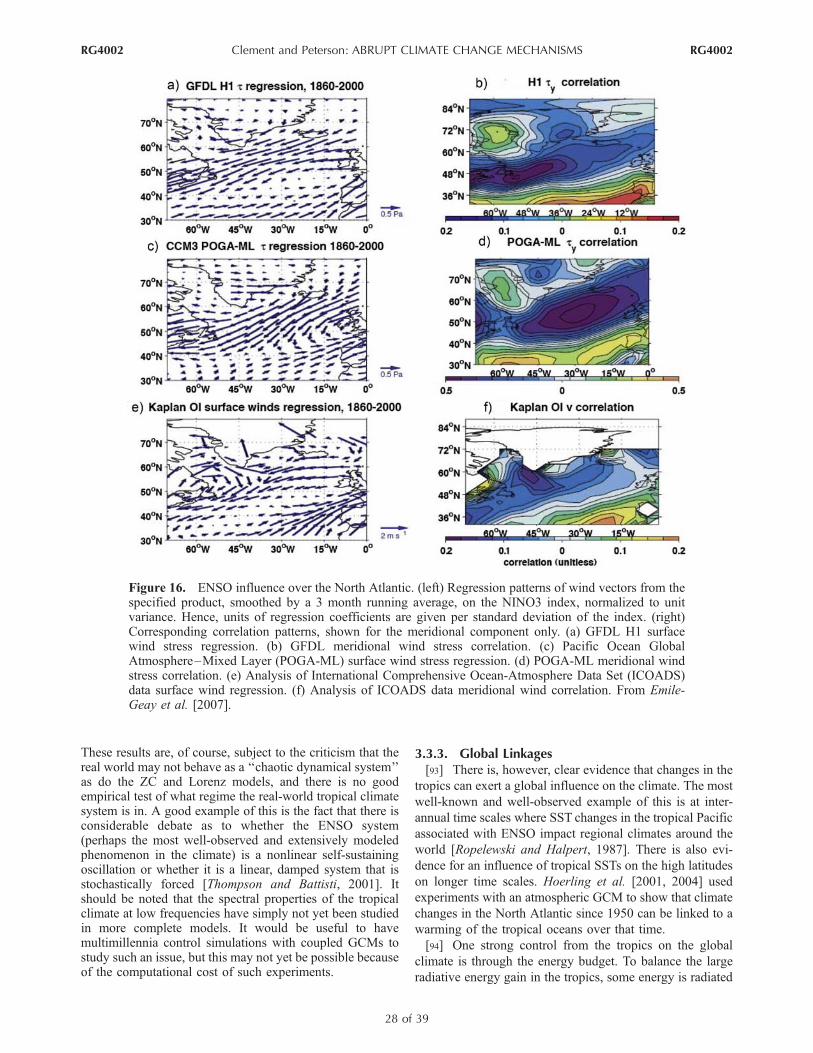
These results are, of course, subject to the criticism that thereal world may not behave as a ‘‘chaotic dynamical system’’as do the ZC and Lorenz models, and there is no goodempirical test of what regime the real-world tropical climatesystem is in. A good example of this is the fact that there isconsiderable debate as to whether the ENSO system(perhaps the most well-observed and extensively modeledphenomenon in the climate) is a nonlinear self-sustainingoscillation or whether it is a linear, damped system that isstochastically forced [Thompson and Battisti, 2001]. Itshould be noted that the spectral properties of the tropicalclimate at low frequencies have simply not yet been studiedin more complete models. It would be useful to havemultimillennia control simulations with coupled GCMs tostudy such an issue, but this may not yet be possible becauseof the computational cost of such experiments.

3.3.3. Global Linkages[93] There is, however, clear evidence that changes in the

tropics can exert a global influence on the climate. The most

well-known and well-observed example of this is at inter-

annual time scales where SST changes in the tropical Pacific

associated with ENSO impact regional climates around the

world [Ropelewski and Halpert, 1987]. There is also evi-

dence for an influence of tropical SSTs on the high latitudes

on longer time scales. Hoerling et al. [2001, 2004] used

experiments with an atmospheric GCM to show that climate

changes in the North Atlantic since 1950 can be linked to a

warming of the tropical oceans over that time.

[94] One strong control from the tropics on the global

climate is through the energy budget. To balance the large

radiative energy gain in the tropics, some energy is radiated

Figure 16. ENSO influence over the North Atlantic. (left) Regression patterns of wind vectors from thespecified product, smoothed by a 3 month running average, on the NINO3 index, normalized to unitvariance. Hence, units of regression coefficients are given per standard deviation of the index. (right)Corresponding correlation patterns, shown for the meridional component only. (a) GFDL H1 surfacewind stress regression. (b) GFDL meridional wind stress correlation. (c) Pacific Ocean GlobalAtmosphere–Mixed Layer (POGA-ML) surface wind stress regression. (d) POGA-ML meridional windstress correlation. (e) Analysis of International Comprehensive Ocean-Atmosphere Data Set (ICOADS)data surface wind regression. (f) Analysis of ICOADS data meridional wind correlation. From Emile-Geay et al. [2007].

RG4002 Clement and Peterson: ABRUPT CLIMATE CHANGE MECHANISMS

28 of 39

RG4002

locally to space, and the residual is exported to and warms

the high latitudes. Pierrehumbert [1995, 2000] suggested

that one of the main controls on the tropical radiative

balance (and hence what is available for export) is the water

vapor content of the subtropical free troposphere (i.e., above

the convective boundary layer). First, he argues that the

existence of this dry region is essential to maintain energy

balance in the tropics. Without these regions in which the

clear-sky outgoing longwave radiation (OLR) is high, the

tropics would be in a state of runaway greenhouse. The

clear-sky OLR is related to both the temperature and water

vapor content of the atmosphere. If, for example, a surface

warming were to moisten the subtropical atmosphere, this

would lead to a reduction in OLR and provide a strong

amplifier for the warming. There are still large uncertainties

in what determines the water vapor content of the subtrop-

ical troposphere [Held and Soden, 2000], but it is now quite

clear from satellite observations that water vapor is acting as

a positive feedback in the global mean warming of the last

several decades [Soden et al., 2005]. It has also been shown

that a transition from a La Nina– to an El Nino–like mean

tropical state does significantly increase the net amount of

water vapor in the troposphere contributing to net warming

of the Earth’s surface [Barreiro et al., 2006]. These ideas

suggest that a perturbation to the tropical climate that

influences the water vapor content could be strongly am-

plified and lead to a globally synchronous warming or

cooling.

[95] Another way to perturb the tropical energy balance is

via changes in subtropical stratocumulus clouds. These

clouds have a significant cooling effect on the climate

because they have a high albedo, but they do not affect

the OLR much because they are low and have cloud top

temperatures that are close to the surface temperature

[Hartmann et al., 1992]. A perturbation to the tropical

climate that alters the amount or spatial extent of these

clouds would also lead to a global cooling or warming [e.g.,

Miller, 1997; Clement and Seager, 1999; Clement and

Soden, 2005; Barreiro et al., 2006]. However, it is not well

known what controls the low cloud cover even for the

modern climate, and it remains difficult to simulate these

clouds in climate models [Bretherton, 2007]. Another

limitation to the arguments suggesting a potential role for

water vapor and low clouds is that those processes are likely

to affect the tropical or global mean temperature, yet it

remains to be seen to what extent the abrupt events of the

last glacial are associated with a mean temperature change.

[96] A second idea derives from the example of modern

teleconnections from the tropics [e.g., Ropelewski and

Halpert, 1987], but this phenomenon is explored under

glacial climate conditions during which the largest known

abrupt climate changes occurred. Yin and Battisti [2001]

performed a number of experiments with an atmospheric

GCM in which the glacial SSTs were specified at values

indicated by CLIMAP Project Members [1981]. The LGM

boundary conditions for ice sheet elevation and extent (from

the Peltier [1994] reconstruction), the seasonally varying

insolation (calculated for 21 ka B.P.), and the concentrations

of greenhouse gases (including a LGM CO2 concentration

of 200 ppm) were also prescribed. Yin and Battisti found

that slight changes in the pattern of SST change in the

tropical Pacific had a large impact on the temperature at the

southern boundary of the Laurentide Ice Sheet and on its

annual mean mass balance. Because meltwater from the

Laurentide Ice Sheet is often suggested as playing a role in

NADW formation, it could be argued that this is a mech-

anism for the tropical Pacific to influence the North Atlantic

Ocean. However, Yin and Battisti point out that this large

sensitivity to SST pattern, in particular SST gradients,

implies that the spatial pattern of SST change must be

known in detail in order to evaluate its impacts outside

the tropics. As noted in section 2, the current paleodata

coverage in the tropics is far from being able to address this

issue. Hence, all that can be said at this point is that it is

physically plausible that changes in the tropical SST influ-

ence the Laurentide Ice Sheet mass balance.

[97] Another teleconnection has been postulated linking

the tropical Pacific and North Atlantic wind patterns. Emile-

Geay et al. [2007] have shown that there is a statistically

significant correlation between ENSO and winds flowing

out of Fram Straits in the wintertime. The observed behavior

is also captured in atmospheric GCMs forced by observed

SST, though the simulated connection appears to be some-

what stronger than in observations (Figure 16). Bond et al.

[2001] argued that it is the winds over Fram Straits that

drive sea ice out of the Arctic, causing large-grained sedi-

ments (IRD) to be deposited in the open North Atlantic and

coinciding during the last glacial with abrupt dips in Green-

land temperatures. This atmospheric bridge represents an-

other pathway by which the tropical Pacific can alter the

North Atlantic climate, in particular the ocean, which

should be further explored.

[98] The tropical Pacific can also influence the North

Atlantic Ocean through freshwater transport in the atmo-

sphere. Schmittner et al. [2000] show that there are sizable

interannual variations in the freshwater export from the

tropical Atlantic. In particular, during El Nino events, more

fresh water is removed from the tropical Atlantic Basin. The

exact pathway of this anomalous transport was not identi-

fied and is difficult to show because of the lack of complete

observations of the large-scale circulation and distribution

of water vapor. However, it is well known that there is a

large flux of water vapor carried by easterly airflow over the

Isthmus of Panama [Zaucker et al., 1994], and this is a

likely exit route for Atlantic water vapor. It has been argued

that the changes in freshwater export have implications

downstream for NADW formation. That is, if the mean state

of the tropical Pacific were to shift to a more El Nino–like

state, the atmosphere would export more water vapor from

the tropical Atlantic, which would become saltier. This

would then lead to an increased vigor of deepwater

formation downstream in the North Atlantic. Latif [2003]

suggested that such a mechanism was operating in increas-

ing CO2 experiments with the ECHO-G coupled ocean-

atmosphere GCM. He pointed out that under increased CO2,

the mean state of the tropical Pacific in that model becomes

RG4002 Clement and Peterson: ABRUPT CLIMATE CHANGE MECHANISMS

29 of 39

RG4002

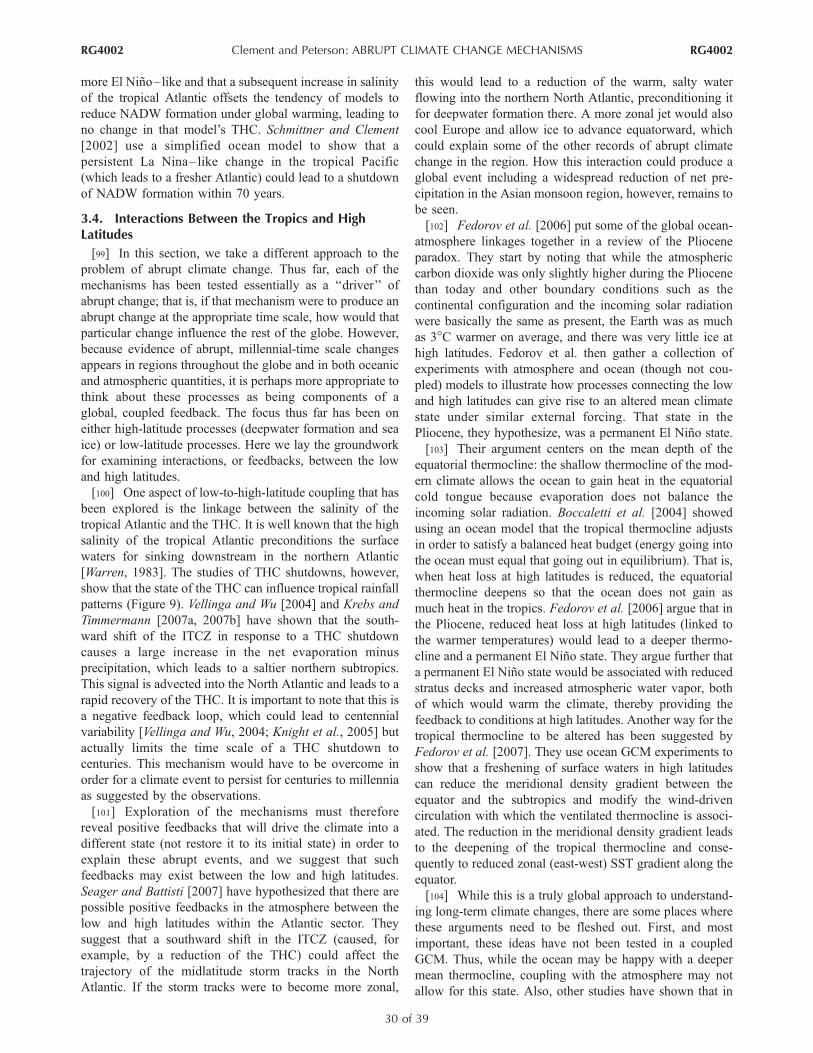
more El Nino–like and that a subsequent increase in salinity

of the tropical Atlantic offsets the tendency of models to

reduce NADW formation under global warming, leading to

no change in that model’s THC. Schmittner and Clement

[2002] use a simplified ocean model to show that a

persistent La Nina– like change in the tropical Pacific

(which leads to a fresher Atlantic) could lead to a shutdown

of NADW formation within 70 years.

3.4. Interactions Between the Tropics and HighLatitudes

[99] In this section, we take a different approach to the

problem of abrupt climate change. Thus far, each of the

mechanisms has been tested essentially as a ‘‘driver’’ of

abrupt change; that is, if that mechanism were to produce an

abrupt change at the appropriate time scale, how would that

particular change influence the rest of the globe. However,

because evidence of abrupt, millennial-time scale changes

appears in regions throughout the globe and in both oceanic

and atmospheric quantities, it is perhaps more appropriate to

think about these processes as being components of a

global, coupled feedback. The focus thus far has been on

either high-latitude processes (deepwater formation and sea

ice) or low-latitude processes. Here we lay the groundwork

for examining interactions, or feedbacks, between the low

and high latitudes.

[100] One aspect of low-to-high-latitude coupling that has

been explored is the linkage between the salinity of the

tropical Atlantic and the THC. It is well known that the high

salinity of the tropical Atlantic preconditions the surface

waters for sinking downstream in the northern Atlantic

[Warren, 1983]. The studies of THC shutdowns, however,

show that the state of the THC can influence tropical rainfall

patterns (Figure 9). Vellinga and Wu [2004] and Krebs and

Timmermann [2007a, 2007b] have shown that the south-

ward shift of the ITCZ in response to a THC shutdown

causes a large increase in the net evaporation minus

precipitation, which leads to a saltier northern subtropics.

This signal is advected into the North Atlantic and leads to a

rapid recovery of the THC. It is important to note that this is

a negative feedback loop, which could lead to centennial

variability [Vellinga and Wu, 2004; Knight et al., 2005] but

actually limits the time scale of a THC shutdown to

centuries. This mechanism would have to be overcome in

order for a climate event to persist for centuries to millennia

as suggested by the observations.

[101] Exploration of the mechanisms must therefore

reveal positive feedbacks that will drive the climate into a

different state (not restore it to its initial state) in order to

explain these abrupt events, and we suggest that such

feedbacks may exist between the low and high latitudes.

Seager and Battisti [2007] have hypothesized that there are

possible positive feedbacks in the atmosphere between the

low and high latitudes within the Atlantic sector. They

suggest that a southward shift in the ITCZ (caused, for

example, by a reduction of the THC) could affect the

trajectory of the midlatitude storm tracks in the North

Atlantic. If the storm tracks were to become more zonal,

this would lead to a reduction of the warm, salty water

flowing into the northern North Atlantic, preconditioning it

for deepwater formation there. A more zonal jet would also

cool Europe and allow ice to advance equatorward, which

could explain some of the other records of abrupt climate

change in the region. How this interaction could produce a

global event including a widespread reduction of net pre-

cipitation in the Asian monsoon region, however, remains to

be seen.

[102] Fedorov et al. [2006] put some of the global ocean-

atmosphere linkages together in a review of the Pliocene

paradox. They start by noting that while the atmospheric

carbon dioxide was only slightly higher during the Pliocene

than today and other boundary conditions such as the

continental configuration and the incoming solar radiation

were basically the same as present, the Earth was as much

as 3�C warmer on average, and there was very little ice at

high latitudes. Fedorov et al. then gather a collection of

experiments with atmosphere and ocean (though not cou-

pled) models to illustrate how processes connecting the low

and high latitudes can give rise to an altered mean climate

state under similar external forcing. That state in the

Pliocene, they hypothesize, was a permanent El Nino state.

[103] Their argument centers on the mean depth of the

equatorial thermocline: the shallow thermocline of the mod-

ern climate allows the ocean to gain heat in the equatorial

cold tongue because evaporation does not balance the

incoming solar radiation. Boccaletti et al. [2004] showed

using an ocean model that the tropical thermocline adjusts

in order to satisfy a balanced heat budget (energy going into

the ocean must equal that going out in equilibrium). That is,

when heat loss at high latitudes is reduced, the equatorial

thermocline deepens so that the ocean does not gain as

much heat in the tropics. Fedorov et al. [2006] argue that in

the Pliocene, reduced heat loss at high latitudes (linked to

the warmer temperatures) would lead to a deeper thermo-

cline and a permanent El Nino state. They argue further that

a permanent El Nino state would be associated with reduced

stratus decks and increased atmospheric water vapor, both

of which would warm the climate, thereby providing the

feedback to conditions at high latitudes. Another way for the

tropical thermocline to be altered has been suggested by

Fedorov et al. [2007]. They use ocean GCM experiments to

show that a freshening of surface waters in high latitudes

can reduce the meridional density gradient between the

equator and the subtropics and modify the wind-driven

circulation with which the ventilated thermocline is associ-

ated. The reduction in the meridional density gradient leads

to the deepening of the tropical thermocline and conse-

quently to reduced zonal (east-west) SST gradient along the

equator.

[104] While this is a truly global approach to understand-

ing long-term climate changes, there are some places where

these arguments need to be fleshed out. First, and most

important, these ideas have not been tested in a coupled

GCM. Thus, while the ocean may be happy with a deeper

mean thermocline, coupling with the atmosphere may not

allow for this state. Also, other studies have shown that in

RG4002 Clement and Peterson: ABRUPT CLIMATE CHANGE MECHANISMS

30 of 39

RG4002

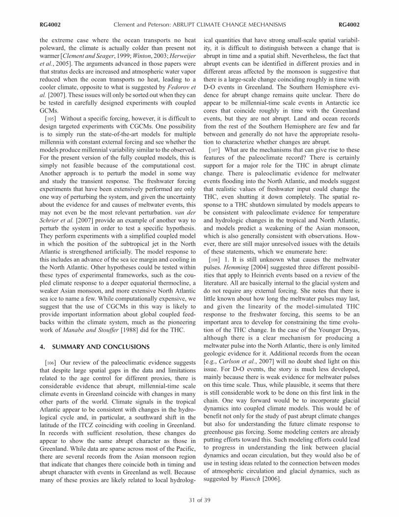
the extreme case where the ocean transports no heat

poleward, the climate is actually colder than present not

warmer [Clement and Seager, 1999;Winton, 2003;Herweijer

et al., 2005]. The arguments advanced in those papers were

that stratus decks are increased and atmospheric water vapor

reduced when the ocean transports no heat, leading to a

cooler climate, opposite to what is suggested by Fedorov et

al. [2007]. These issues will only be sorted out when they can

be tested in carefully designed experiments with coupled

GCMs.

[105] Without a specific forcing, however, it is difficult to

design targeted experiments with CGCMs. One possibility

is to simply run the state-of-the-art models for multiple

millennia with constant external forcing and see whether the

models producemillennial variability similar to the observed.

For the present version of the fully coupled models, this is

simply not feasible because of the computational cost.

Another approach is to perturb the model in some way

and study the transient response. The freshwater forcing

experiments that have been extensively performed are only

one way of perturbing the system, and given the uncertainty

about the evidence for and causes of meltwater events, this

may not even be the most relevant perturbation. van der

Schrier et al. [2007] provide an example of another way to

perturb the system in order to test a specific hypothesis.

They perform experiments with a simplified coupled model

in which the position of the subtropical jet in the North

Atlantic is strengthened artificially. The model response to

this includes an advance of the sea ice margin and cooling in

the North Atlantic. Other hypotheses could be tested within

these types of experimental frameworks, such as the cou-

pled climate response to a deeper equatorial thermocline, a

weaker Asian monsoon, and more extensive North Atlantic

sea ice to name a few. While computationally expensive, we

suggest that the use of CGCMs in this way is likely to

provide important information about global coupled feed-

backs within the climate system, much as the pioneering

work of Manabe and Stouffer [1988] did for the THC.

4. SUMMARY AND CONCLUSIONS

[106] Our review of the paleoclimatic evidence suggests

that despite large spatial gaps in the data and limitations

related to the age control for different proxies, there is

considerable evidence that abrupt, millennial-time scale

climate events in Greenland coincide with changes in many

other parts of the world. Climate signals in the tropical

Atlantic appear to be consistent with changes in the hydro-

logical cycle and, in particular, a southward shift in the

latitude of the ITCZ coinciding with cooling in Greenland.

In records with sufficient resolution, these changes do

appear to show the same abrupt character as those in

Greenland. While data are sparse across most of the Pacific,

there are several records from the Asian monsoon region

that indicate that changes there coincide both in timing and

abrupt character with events in Greenland as well. Because

many of these proxies are likely related to local hydrolog-

ical quantities that have strong small-scale spatial variabil-

ity, it is difficult to distinguish between a change that is

abrupt in time and a spatial shift. Nevertheless, the fact that

abrupt events can be identified in different proxies and in

different areas affected by the monsoon is suggestive that

there is a large-scale change coinciding roughly in time with

D-O events in Greenland. The Southern Hemisphere evi-

dence for abrupt change remains quite unclear. There do

appear to be millennial-time scale events in Antarctic ice

cores that coincide roughly in time with the Greenland

events, but they are not abrupt. Land and ocean records

from the rest of the Southern Hemisphere are few and far

between and generally do not have the appropriate resolu-

tion to characterize whether changes are abrupt.

[107] What are the mechanisms that can give rise to these

features of the paleoclimate record? There is certainly

support for a major role for the THC in abrupt climate

change. There is paleoclimatic evidence for meltwater

events flooding into the North Atlantic, and models suggest

that realistic values of freshwater input could change the

THC, even shutting it down completely. The spatial re-

sponse to a THC shutdown simulated by models appears to

be consistent with paleoclimate evidence for temperature

and hydrologic changes in the tropical and North Atlantic,

and models predict a weakening of the Asian monsoon,

which is also generally consistent with observations. How-

ever, there are still major unresolved issues with the details

of these statements, which we enumerate here:

[108] 1. It is still unknown what causes the meltwater

pulses. Hemming [2004] suggested three different possibil-

ities that apply to Heinrich events based on a review of the

literature. All are basically internal to the glacial system and

do not require any external forcing. She notes that there is

little known about how long the meltwater pulses may last,

and given the linearity of the model-simulated THC

response to the freshwater forcing, this seems to be an

important area to develop for constraining the time evolu-

tion of the THC change. In the case of the Younger Dryas,

although there is a clear mechanism for producing a

meltwater pulse into the North Atlantic, there is only limited

geologic evidence for it. Additional records from the ocean

[e.g., Carlson et al., 2007] will no doubt shed light on this

issue. For D-O events, the story is much less developed,

mainly because there is weak evidence for meltwater pulses

on this time scale. Thus, while plausible, it seems that there

is still considerable work to be done on this first link in the

chain. One way forward would be to incorporate glacial

dynamics into coupled climate models. This would be of

benefit not only for the study of past abrupt climate changes

but also for understanding the future climate response to

greenhouse gas forcing. Some modeling centers are already

putting efforts toward this. Such modeling efforts could lead

to progress in understanding the link between glacial

dynamics and ocean circulation, but they would also be of

use in testing ideas related to the connection between modes

of atmospheric circulation and glacial dynamics, such as

suggested by Wunsch [2006].

RG4002 Clement and Peterson: ABRUPT CLIMATE CHANGE MECHANISMS

31 of 39

RG4002

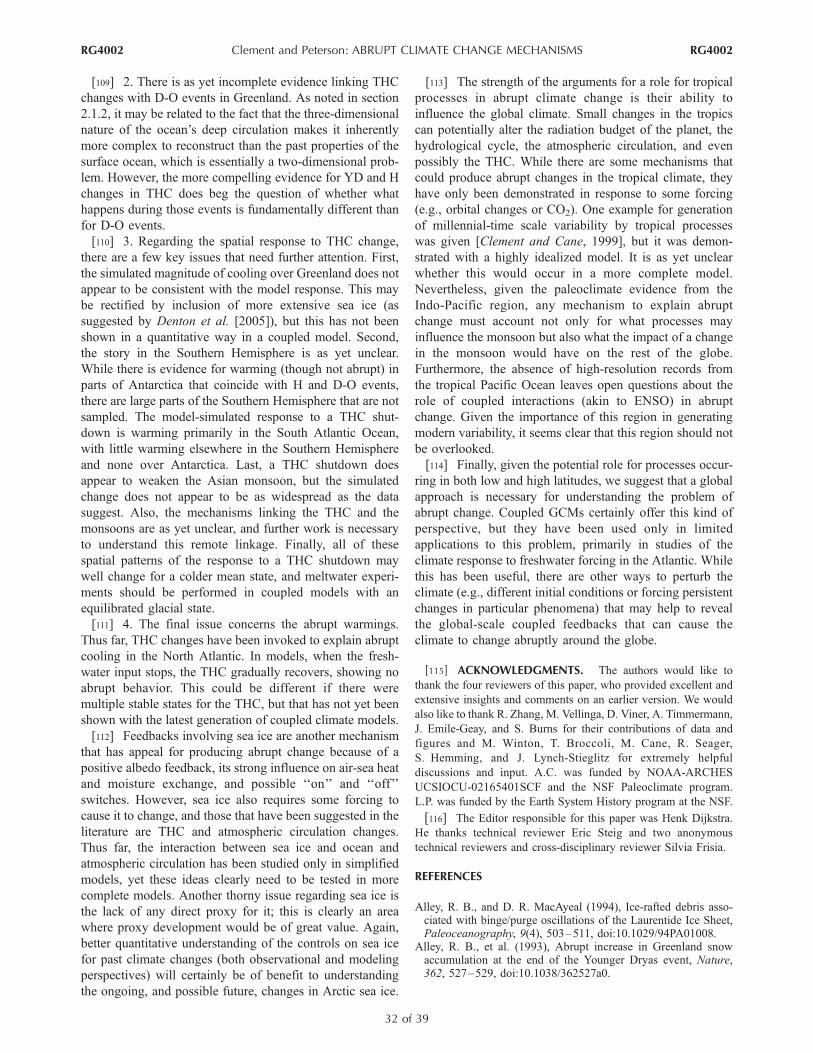
[109] 2. There is as yet incomplete evidence linking THC

changes with D-O events in Greenland. As noted in section

2.1.2, it may be related to the fact that the three-dimensional

nature of the ocean’s deep circulation makes it inherently

more complex to reconstruct than the past properties of the

surface ocean, which is essentially a two-dimensional prob-

lem. However, the more compelling evidence for YD and H

changes in THC does beg the question of whether what

happens during those events is fundamentally different than

for D-O events.

[110] 3. Regarding the spatial response to THC change,

there are a few key issues that need further attention. First,

the simulated magnitude of cooling over Greenland does not

appear to be consistent with the model response. This may

be rectified by inclusion of more extensive sea ice (as

suggested by Denton et al. [2005]), but this has not been

shown in a quantitative way in a coupled model. Second,

the story in the Southern Hemisphere is as yet unclear.

While there is evidence for warming (though not abrupt) in

parts of Antarctica that coincide with H and D-O events,

there are large parts of the Southern Hemisphere that are not

sampled. The model-simulated response to a THC shut-

down is warming primarily in the South Atlantic Ocean,

with little warming elsewhere in the Southern Hemisphere

and none over Antarctica. Last, a THC shutdown does

appear to weaken the Asian monsoon, but the simulated

change does not appear to be as widespread as the data

suggest. Also, the mechanisms linking the THC and the

monsoons are as yet unclear, and further work is necessary

to understand this remote linkage. Finally, all of these

spatial patterns of the response to a THC shutdown may

well change for a colder mean state, and meltwater experi-

ments should be performed in coupled models with an

equilibrated glacial state.

[111] 4. The final issue concerns the abrupt warmings.

Thus far, THC changes have been invoked to explain abrupt

cooling in the North Atlantic. In models, when the fresh-

water input stops, the THC gradually recovers, showing no

abrupt behavior. This could be different if there were

multiple stable states for the THC, but that has not yet been

shown with the latest generation of coupled climate models.

[112] Feedbacks involving sea ice are another mechanism

that has appeal for producing abrupt change because of a

positive albedo feedback, its strong influence on air-sea heat

and moisture exchange, and possible ‘‘on’’ and ‘‘off’’

switches. However, sea ice also requires some forcing to

cause it to change, and those that have been suggested in the

literature are THC and atmospheric circulation changes.

Thus far, the interaction between sea ice and ocean and

atmospheric circulation has been studied only in simplified

models, yet these ideas clearly need to be tested in more

complete models. Another thorny issue regarding sea ice is

the lack of any direct proxy for it; this is clearly an area

where proxy development would be of great value. Again,

better quantitative understanding of the controls on sea ice

for past climate changes (both observational and modeling

perspectives) will certainly be of benefit to understanding

the ongoing, and possible future, changes in Arctic sea ice.

[113] The strength of the arguments for a role for tropical

processes in abrupt climate change is their ability to

influence the global climate. Small changes in the tropics

can potentially alter the radiation budget of the planet, the

hydrological cycle, the atmospheric circulation, and even

possibly the THC. While there are some mechanisms that

could produce abrupt changes in the tropical climate, they

have only been demonstrated in response to some forcing

(e.g., orbital changes or CO2). One example for generation

of millennial-time scale variability by tropical processes

was given [Clement and Cane, 1999], but it was demon-

strated with a highly idealized model. It is as yet unclear

whether this would occur in a more complete model.

Nevertheless, given the paleoclimate evidence from the

Indo-Pacific region, any mechanism to explain abrupt

change must account not only for what processes may

influence the monsoon but also what the impact of a change

in the monsoon would have on the rest of the globe.

Furthermore, the absence of high-resolution records from

the tropical Pacific Ocean leaves open questions about the

role of coupled interactions (akin to ENSO) in abrupt

change. Given the importance of this region in generating

modern variability, it seems clear that this region should not

be overlooked.

[114] Finally, given the potential role for processes occur-

ring in both low and high latitudes, we suggest that a global

approach is necessary for understanding the problem of

abrupt change. Coupled GCMs certainly offer this kind of

perspective, but they have been used only in limited

applications to this problem, primarily in studies of the

climate response to freshwater forcing in the Atlantic. While

this has been useful, there are other ways to perturb the

climate (e.g., different initial conditions or forcing persistent

changes in particular phenomena) that may help to reveal

the global-scale coupled feedbacks that can cause the

climate to change abruptly around the globe.

[115] ACKNOWLEDGMENTS. The authors would like to

thank the four reviewers of this paper, who provided excellent and

extensive insights and comments on an earlier version. We would

also like to thank R. Zhang, M. Vellinga, D. Viner, A. Timmermann,

J. Emile-Geay, and S. Burns for their contributions of data and

figures and M. Winton, T. Broccoli, M. Cane, R. Seager,

S. Hemming, and J. Lynch-Stieglitz for extremely helpful

discussions and input. A.C. was funded by NOAA-ARCHES

UCSIOCU-02165401SCF and the NSF Paleoclimate program.

L.P. was funded by the Earth System History program at the NSF.

[116] The Editor responsible for this paper was Henk Dijkstra.

He thanks technical reviewer Eric Steig and two anonymous

technical reviewers and cross-disciplinary reviewer Silvia Frisia.

REFERENCES

Alley, R. B., and D. R. MacAyeal (1994), Ice-rafted debris asso-ciated with binge/purge oscillations of the Laurentide Ice Sheet,Paleoceanography, 9(4), 503–511, doi:10.1029/94PA01008.

Alley, R. B., et al. (1993), Abrupt increase in Greenland snowaccumulation at the end of the Younger Dryas event, Nature,362, 527–529, doi:10.1038/362527a0.

RG4002 Clement and Peterson: ABRUPT CLIMATE CHANGE MECHANISMS

32 of 39

RG4002

Alley, R. B., D. A. Shuman, A. J. Gow, K. C. Taylor, J. J. Cuffey,P. M. Fitzpatrick, G. A. Zielinski, M. Ram, G. Spinelli, andB. Elder (1997), Visual stratigraphic dating of the GISP2 icecore: Basis, reproducibility, and application, J. Geophys. Res.,102(C12), 26,367–26,381, doi:10.1029/96JC03837.

Alley, R., P. U. Clark, L. D. Keigwin, and R. S. Webb (1999),Making sense of millennial-scale climate change, in Mechanismsof Global Climate Change at Millennial Time Scales, Geophys.Monogr. Ser., vol. 112, edited by P. U. Clark, R. S. Webb, andL. D. Keigwin, pp. 385–394, AGU, Washington, D. C.

Alley, R. B., S. Anandakrishnan, and P. Jung (2001), Stochasticresonance in the North Atlantic, Paleoceanography, 16(2), 190–198, doi:10.1029/2000PA000518.

Altabet, M. A., M. J. Higginson, and D. W. Murray (2002), Theeffect of millennial-scale changes in Arabian Sea denitrificationon atmospheric CO2, Nature, 415, 159–162, doi:10.1038/415159a.

Arz, H. W., J. Patzold, and G. Wefer (1998), Correlated millennial-scale changes in surface hydrography and terrigenous sedimentyield inferred from last-glacial marine deposits off Brazil, Quat.Res., 50, 157–166, doi:10.1006/qres.1998.1992.

Baker, P. A., C. A. Rigsby, G. O. Seltzer, S. C. Fritz, T. K.Lowenstein, N. P. Bacher, and C. Veliz (2001), Tropical climatechanges at millennial and orbital timescales on the BolivianAltiplano, Nature, 409, 698–700, doi:10.1038/35055524.

Bakun, A., and K. Broad (2003), Environmental ‘loopholes’ andfish population dynamics: Comparative pattern recognition withfocus on El Nino effects in the Pacific, Fish. Oceanogr., 12,458–473, doi:10.1046/j.1365-2419.2003.00258.x.

Bard, E., R. Rostek, J.-L. Turon, and S. Gendreau (2000), Hydrolo-gical impact of Heinrich events in the subtropical northeast Atlantic,Science, 289, 1321–1324, doi:10.1126/science.289.5483.1321.

Barnett, T. P., L. Dumenil, U. Schlese, and E. Roeckner (1988),The effect of Eurasian snow cover on global climate, Science,239, 504–507, doi:10.1126/science.239.4839.504.

Barnett, T. P., D. W. Pierce, M. Latif, D. Dommenget, andR. Saravanan (1999), Interdecadal interactions between the tro-pics and midlatitudes in the Pacific Basin, Geophys. Res. Lett.,26, 615–618, doi:10.1029/1999GL900042.

Barreiro, M., et al. (2006), Simulations of warm tropical conditionswith application to middle Pliocene atmospheres, Clim. Dyn., 26,349–365, doi:10.1007/s00382-005-0086-4.

Behl, R. J., and J. P. Kennett (1996), Brief interstadial events in theSanta Barbara Basin, NE Pacific, during the past 60 kyr, Nature,379, 243–246, doi:10.1038/379243a0.

Bennett, K. D., S. G. Haberle, and S. H. Lumley (2000), The lastglacial-Holocene transition in southern Chile, Science, 290,325–328, doi:10.1126/science.290.5490.325.

Black, D. E., L. C. Peterson, J. T. Overpeck, A. Kaplan, M. N.Evans, and M. Kashgarian (1999), Eight centuries of NorthAtlantic ocean atmosphere variability, Science, 286, 1709–1713, doi:10.1126/science.286.5445.1709.

Blunier, T., and E. J. Brook (2001), Timing of millennial-scale cli-mate change in Antarctica and Greenland during the last glacialperiod, Science , 291 , 109 – 112, doi:10.1126/science.291.5501.109.

Blunier, T., et al. (1998), Asynchrony of Antarctic and Greenlandclimate change during the last glacial period, Nature, 394, 739–743, doi:10.1038/29447.

Boccaletti, G., R. C. Pacanowski, S. George, H. Philander, andA. V. Fedorov (2004), The thermal structure of the upper ocean,J. Phys. Oceanogr. , 34 , 888 – 902, doi:10.1175/1520-0485(2004)034<0888:TTSOTU>2.0.CO;2.

Bond, G., et al. (1992), Evidence for massive discharges of ice-bergs into the North Atlantic ocean during the last glacial period,Nature, 360, 245–249, doi:10.1038/360245a0.

Bond, G., W. Broecker, S. Johnsen, J. McManus, L. Labeyrie,J. Jouzel, and G. Bonani (1993), Correlations between climaterecords from North Atlantic sediments and Greenland ice, Nat-ure, 365, 143–147, doi:10.1038/365143a0.

Bond, G., et al. (2001), Persistent solar influence on North Atlanticclimate during the Holocene, Science, 294, 2130 – 2136,doi:10.1126/science.1065680.

Boyle, E. A., and L. D. Keigwin (1987), North Atlantic thermoha-line circulation during the last 20,000 years linked to high-latitudesurface temperature, Nature, 330, 35–40, doi:10.1038/330035a0.

Braun, H., M. Christl, S. Rahmstorf, A. Ganopolski, A. Mangini,C. Kubatzki, K. Roth, and B. Kromer (2005), Possible solar originof the 1470-year glacial climate cycle demonstrated in a coupledmodel, Nature, 438, 208–211, doi:10.1038/nature04121.

Bretherton, C. S. (2007), Challenges in numerical modeling oftropical circulations, in The Global Circulation of the Atmo-sphere, edited by T. Schneider and A. H. Sobel, pp. 302–330,Princeton Univ. Press, Princeton, N. J.

Broccoli, A. J., K. A. Dahl, and R. J. Stouffer (2006), Response ofthe ITCZ to Northern Hemisphere cooling, Geophys. Res. Lett.,33, L01702, doi:10.1029/2005GL024546.

Broecker, W. S. (1998), Paleocean circulation during the last de-glaciation: A bipolar seesaw?, Paleoceanography, 13(2), 119–121, doi:10.1029/97PA03707.

Broecker, W. S. (2006a), Was the Younger Dryas triggered by aflood?, Science, 312, 1146–1148, doi:10.1126/science.1123253.

Broecker, W. S. (2006b), Abrupt climate change revisited, GlobalPlanet. Change, 54(3–4), 211–215, doi:10.1016/j.gloplacha.2006.06.019.

Broecker, W., and S. Barker (2007), A 190% drop in atmosphere’sD14C during the ‘‘Mystery Interval’’ (17.5 to 14.5 kyr), EarthPlanet. Sci. Lett., 256, 90–99, doi:10.1016/j.epsl.2007.01.015.

Broecker, W. S., and S. Hemming (2001), Climate swings comeinto focus , Science , 294 , 2308 – 2309, doi :10.1126/science.1068389.

Broecker, W. S., D. M. Peteet, and D. Rind (1985), Does theocean-atmosphere system have more than one stable mode ofoperation?, Nature, 315, 21–25, doi:10.1038/315021a0.

Broecker, W. S., G. Bond, M. Klas, E. Clark, and J. McManus(1992), Origin of the northern Atlantic’s Heinrich events, Clim.Dyn., 6, 265–273, doi:10.1007/BF00193540.

Brook, E. J., T. Sowers, and J. Orchardo (1996), Rapid variations inatmospheric methane concentration during the past 110,000 years,Science, 273, 1087–1091, doi:10.1126/science.273.5278.1087.

Brook, E., S. Harder, J. Severinghaus, and M. Bender (1999),Atmospheric methane and millennial-scale climate change, inMechanisms of Global Climate Change at Millennial TimeScales, Geophys. Monogr. Ser., vol. 112, edited by P. U. Clark,R. S. Webb, and L. D. Keigwin, pp. 165–175, AGU, Washington,D. C.

Burns, S. J., D. Fleitmann, A. Matter, J. Kramers, and A. A.Al-Subbary (2003), Indian Ocean climate and an absolute chron-ology over Dansgaard/Oeschger events 9 to 13, Science, 301,1365–1367, doi:10.1126/science.1086227.

Cane, M. A. (1998), Climate change: A role for the tropical Pacific,Science, 282, 59–61, doi:10.1126/science.282.5386.59.

Cane, M. A., and A. C. Clement (1999), A role for the tropicalPacific coupled ocean-atmosphere system on Milankovitch andmillennial timescales. Part II: Global impacts, in Mechanisms ofGlobal Climate Change at Millennial Time Scales, Geophys.Monogr. Ser., vol. 112, edited by P. U. Clark, R. S. Webb, andL. D. Keigwin, pp. 373–383, AGU, Washington, D. C.

Carlson, A. E., P. U. Clark, B. A. Haley, G. P. Klinkhammer,K. Simmons, E. J. Brook, and K. J. Meissner (2007), Geochem-ical proxies of North American freshwater routing during theYounger Dryas cold event, Proc. Natl. Acad. Sci. U. S. A.,104, 6556–6561, doi:10.1073/pnas.0611313104.

Cessi, P., K. Bryan, and R. Zhang (2004), Global seiching ofthermocline waters between the Atlantic and the Indian-PacificOcean basins, Geophys. Res. Lett., 31, L04302, doi:10.1029/2003GL019091.

Chang, P., B. Wang, T. Li, and L. Ji (1994), Interactions between theseasonal cycle and the Southern Oscillation-frequency entrain-

RG4002 Clement and Peterson: ABRUPT CLIMATE CHANGE MECHANISMS

33 of 39

RG4002

ment and chaos in a coupled ocean-atmosphere model, Geophys.Res. Lett., 21, 2817–2820, doi:10.1029/94GL02759.

Charles, C. D., J. Lynch-Stieglitz, U. S. Ninnemann, and R. G.Fairbanks (1996), Climate connections between the hemispheresrevealed by deep sea sediment core/ice core correlations, EarthPlanet. Sci. Lett., 142, 19 – 27, doi:10.1016/0012-821X(96)00083-0.

Chiang, J. C. H., and C. M. Bitz (2005), Influence of high latitudeice cover on the marine Intertropical Convergence Zone, Clim.Dyn., 25, 477–496, doi:10.1007/s00382-005-0040-5.

Chiang, J. C. H., and D. J. Vimont (2004), Analogous Pacific andAtlantic meridional modes of tropical atmosphere-ocean varia-bility, J. Clim., 17, 4143–4158, doi:10.1175/JCLI4953.1.

Chiang, J. C. H., M. Biasutti, and D. S. Battisti (2003), Sensitivityof the Atlantic Intertropical Convergence Zone to Last GlacialMaximum boundary conditions, Paleoceanography, 18(4), 1094,doi:10.1029/2003PA000916.

Clark, P. U., S. J. Marshall, G. K. C. Clarke, S. W. Hostetler, J. M.Licciardi, and J. T. Teller (2001), Freshwater forcing of abruptclimate change during the last glaciation, Science, 293, 283–287,doi:10.1126/science.1062517.

Clark, P. U., N. G. Pisias, T. F. Stocker, and A. J. Weaver (2002),The role of the thermohaline circulation in abrupt climatechange, Nature, 415, 863–869, doi:10.1038/415863.

Clement, A. C., and M. A. Cane (1999), A role for the tropicalPacific coupled ocean-atmosphere system on Milankovitch andmillennial timescales. Part I: A modeling study of tropicalPacific variability, in Mechanisms of Global Climate Changeat Millennial Time Scales,Geophys. Monogr. Ser., vol. 112, editedby P. U. Clark, R. S. Webb, and L. D. Keigwin, pp. 363–371,AGU, Washington, D. C.

Clement, A., and R. Seager (1999), Climate and the tropical oceans,J. Clim., 12, 3383–3401, doi:10.1175/1520-0442(1999)012<3383:CATTO>2.0.CO;2.

Clement, A. C., and B. Soden (2005), The sensitivity of the tropi-cal-mean radiation budget, J. Clim., 18 , 3189 – 3203,doi:10.1175/JCLI3456.1.

Clement, A. C., R. Seager, and M. A. Cane (1999), Orbital controlson ENSO and the tropical climate, Paleoceanography, 14, 441–456.

Clement, A. C., M. A. Cane, and R. Seager (2001), An orbitallydriven tropical source for abrupt climate change, J. Clim., 14,2369 – 2375, doi:10.1175/1520-0442(2001)014<2369:AODTSF> 2.0.CO;2.

CLIMAP Project Members (1981), Seasonal reconstructions of theEarth’s surface at the Last Glacial Maximum, Geol. Soc. Am.Map Chart Ser., MC-36.

Crowley, T. J. (1992), North Atlantic Deep Water cools the South-ern Hemisphere, Paleoceanography, 7(4), 489 – 497,doi:10.1029/92PA01058.

Crowley, T. J. (2000), CLIMAP SSTs re-visited, Clim. Dyn., 16,241–255, doi:10.1007/s003820050325.

Cruz, F. W., S. J. Burns, I. Karmann, W. D. Sharp, M. Vuille,A. Cardoso, J. Ferrari, P. Silva Dias, and O. Viana (2005),Insolation-driven changes in atmospheric circulation over thepast 116000 years in subtropical Brazil, Nature, 434, 63–66,doi:10.1038/nature03365.

Cuffey, K. M., and G. D. Clow (1997), Temperature, accumulation,and ice sheet elevation in central Greenland through the lastdeglacial transition, J. Geophys. Res., 102(C12), 26,383–26,396, doi:10.1029/96JC03981.

Curry, W. B., T. M. Marchitto, J. F. McManus, D. W. Oppo, andK. L. Laarkamp (1999), Millennial-scale changes in ventilationof the thermocline, intermediate and deep waters of the glacialNorth Atlantic, in Mechanisms of Global Climate Change atMillennial Time Scales, Geophys. Monogr. Ser., vol. 112, editedby P. U. Clark, R. S. Webb, and L. D. Keigwin, pp. 59–76,AGU, Washington, D. C.

Dannenmann, S., B. K. Linsley, D. W. Oppo, Y. Rosenthal, andL. Beaufort (2003), East Asian monsoon forcing of suborbital

variability in the Sulu Sea during marine isotope stage 3: Linkto Northern Hemisphere climate, Geochem. Geophys. Geosyst.,4(1), 1001, doi:10.1029/2002GC000390.

Dansgaard, W., S. J. Johnsen, H. B. Clausen, D. Dahl-Jensen,N. Gundestrup, C. U. Hammer, and H. Oeschger (1984), NorthAtlantic climatic oscillations revealed by deep Greenland icecores, in Climate Processes and Climate Sensitivity, Geophys.Monogr. Ser., vol. 29, edited by J. E. Hansen and T. Takahashi,pp. 288–298, AGU, Washington, D. C.

Dansgaard, W., et al. (1993), Evidence for general instability ofpast climate from a 250-kyr ice core record, Nature, 364, 218–220, doi:10.1038/364218a0.

Delworth, T. L., et al. (2006), GFDL’s CM2 global coupled climatemodels. Part I: Formulation and simulation characteristics,J. Clim., 19, 643–674, doi:10.1175/JCLI3629.1.

Denton, G. H., and C. H. Hendy (1994), Younger Dryas age advanceof Franz Josef Glacier in the Southern Alps of New Zealand,Science, 264, 1434–1437, doi:10.1126/science.264.5164.1434.

Denton, G. H., R. B. Alley, G. C. Comer, and W. S. Broecker(2005), The role of seasonality in abrupt climate change, Quat.Sci. Rev., 24, 1159–1182, doi:10.1016/j.quascirev.2004.12.002.

Deser, C., A. S. Phillips, and J. W. Hurrell (2004), Pacific interde-cadal climate variability: Linkages between the tropics and theNorth Pacific during boreal winter since 1900, J. Clim., 17,3109 – 3124, doi:10.1175/1520-0442(2004)017<3109:PICVLB>2.0.CO;2.

de Vernal, A., and C. Hillaire-Marcel (2000), Sea-ice cover, sea-surface salinity and halo-thermocline structure of the northwestNorth Atlantic: Modern versus full glacial conditions, Quat. Sci.Rev., 19, 65–85, doi:10.1016/S0277-3791(99)00055-4.

Dong, B.-W., and R. T. Sutton (2002), Adjustment of the coupledocean–atmosphere system to a sudden change in the thermoha-line circulation, Geophys. Res. Lett., 29(15), 1728, doi:10.1029/2002GL015229.

Dutton, J. F., C. J. Poulsen, and J. L. Evans (2000), The effect of globalclimate change on the regions of tropical convection in CSM1,Geophys. Res. Lett., 27, 3049–3052, doi:10.1029/2000GL011542.

Elliot, M., L. Labeyrie, and C. J.-Duplessy (2002), Changes inNorth Atlantic deep-water formation associated with the Dans-gaard-Oeschger temperature oscillations (60–10 ka), Quat. Sci.Rev., 21, 1153–1165, doi:10.1016/S0277-3791(01)00137-8.

Emile-Geay, J., M. Cane, R. Seager, A. Kaplan, and P. Almasi(2007), El Nino as a mediator of the solar influence on climate,Paleoceanography, 22, PA3210, doi:10.1029/2006PA001304.

EPICA Community Members (2006), One-to-one coupling of gla-cial climate variability in Greenland and Antarctica, Nature, 444,195–198, doi:10.1038/nature05301.

Fedorov, A. V., et al. (2004), The effect of salinity on the wind-driven circulation and the thermal structure of the upper ocean,J. Phys. Oceanogr., 34, 1949 – 1966, doi:10.1175/1520-0485(2004)034<1949:TEOSOT>2.0.CO;2.

Fedorov, A. V., P. S. Dekens, M. McCarthy, A. C. Ravelo, P. B.deMenocal, M. Barreiro, R. C. Pacanowski, and S. G. Philander(2006), The Pliocene paradox (mechanisms for a permanent ElNino), Science, 312, 1485–1489, doi:10.1126/science.1122666.

Fedorov, A., M. Barreiro, G. Boccaletti, R. Pacanowski, and S. G.Philander (2007), The freshening of surface waters in high lati-tudes: Effects on the thermohaline and wind-driven circulations,J. Phys. Oceanogr., 37, 896–907, doi:10.1175/JPO3033.1.

Fitzsimons, S. J. (1997), Late-glacial and early Holocene glacieractivity in the Southern Alps, New Zealand, Quat. Int., 38-39,69–76, doi:10.1016/S1040-6182(96)00022-5.

Fleitmann, D., S. J. Burns, M. Mudelsee, U. Neff, J. Kramers,A. Mangini, and A. Matter (2003), Holocene forcing of the In-dian monsoon recorded in a stalagmite from southern Oman,Science, 300, 1737–1739, doi:10.1126/science.1083130.

Ganachaud, A., and C. Wunsch (2003), Large-scale ocean heat andfreshwater transports during the World Ocean Circulation Experi-ment, J. Clim., 16, 696–705, doi:10.1175/1520-0442(2003)016<0696:LSOHAF>2.0.CO;2.

RG4002 Clement and Peterson: ABRUPT CLIMATE CHANGE MECHANISMS

34 of 39

RG4002

Ganopolski, A., and S. Rahmstorf (2001), Rapid changes of glacialclimate simulated in a coupled climate model, Nature, 409, 153–158, doi:10.1038/35051500.

Gershunov, A., N. Schneider, and T. Barnett (2001), Low-frequencymodulation of the ENSO-Indian monsoon rainfall relationship:Signal or noise?, J. Clim., 14, 2486–2492, doi:10.1175/1520-0442(2001)014<2486:LFMOTE>2.0.CO;2.

Gherardi, J. M., L. Labeyrie, J. F. McManus, R. Francois, L. C.Skinner, and E. Cortijo (2005), Evidence from the northeasternAtlantic Basin for variability in the rate of the meridional over-turning circulation through the last deglaciation, Earth Planet.Sci. Lett., 240, 710–723, doi:10.1016/j.epsl.2005.09.061.

Gildor, H., and E. Tziperman (2001), A sea ice climate switchmechanism for the 100-kyr glacial cycles, J. Geophys. Res.,106(C5), 9117–9133, doi:10.1029/1999JC000120.

Gildor, H., and E. Tziperman (2003), Sea-ice switches and abruptclimate change, Philos. Trans. R. Soc. London, Ser. A, 361,1935–1942, doi:10.1098/rsta.2003.1244.

Graham, N. E. (1994), Decadal-scale climate variability in thetropical and North Pacific during the 1970s and 1980s: Observa-tions and model results, Clim. Dyn., 10, 135–162, doi:10.1007/BF00210626.

Grimm, E. C., G. L. Jacobsen Jr., W. A. Watts, B. C. S. Hansen,and K. A. Maasch (1993), A 50,000 year record of climateoscillations from Florida and its temporal correlation with theHeinrich events, Science, 261, 198 – 200, doi:10.1126/science.261.5118.198.

Grimm, E. C., W. A. Watts, G. L. Jacobsen Jr., B. C. S. Hansen,H. R. Almquist, and A. C. Dieffenbacher-Krall (2006), Evidencefor warm wet Heinrich events in Florida, Quat. Sci. Rev., 25,2197–2211, doi:10.1016/j.quascirev.2006.04.008.

Grootes, P. M., M. Stuiver, J. W. C. White, S. Johnsen, and J. Jouzel(1993), Comparison of oxygen isotope records from the GISP2and GRIP Greenland ice cores, Nature, 366, 552 – 554,doi:10.1038/366552a0.

Gupta, A. K., D. M. Anderson, and J. T. Overpeck (2003), Abruptchanges in the Asian southwest monsoon during the Holoceneand their links to the North Atlantic Ocean, Nature, 421, 354–356, doi:10.1038/nature01340.

Hagen, S., and L. D. Keigwin (2002), Sea surface temperaturevariability and deep water reorganization in the subtropical NorthAtlantic during isotope stages 2–4, Mar. Geol., 189, 145–162,doi:10.1016/S0025-3227(02)00327-4.

Hartmann, D. L., M. E. Ockert-Bell, and M. L. Michelsen(1992), The effect of cloud type on Earth’s energy balance:Global analysis, J. Clim., 5, 1281–1304, doi:10.1175/1520-0442(1992)005<1281:TEOCTO>2.0.CO;2.

Haug, G. H., K. A. Hughen, D. M. Sigman, L. C. Peterson, andU. Rohl (2001), Southward migration of the Intertropical Con-vergence Zone through the Holocene, Science, 293, 1304–1308, doi:10.1126/science.1059725.

Hazeleger, W., C. Severijns, R. Seager, and F. Molteni (2005),Tropical Pacific–driven decadal energy transport variability,J. Clim., 18, 2037–2051, doi:10.1175/JCLI3389.1.

Heinrich, H. (1988), Origin and consequence of cyclic ice raftingin the northeast Atlantic Ocean during the past 130000 years,Quat. Res., 29, 142–152, doi:10.1016/0033-5894(88)90057-9.

Held, I. M., and B. J. Soden (2000), Water vapor feedback andglobal warming, Annu. Rev. Energy Environ., 25, 441–475,doi:10.1146/annurev.energy.25.1.441.

Hemming, S. (2004), Heinrich events: Massive late Pleistocenedetritus layers of the North Atlantic and their global climateimpr in t , Rev. Geophys . , 42 , RG1005, doi :10 .1029/2003RG000128.

Hendy, I. L., and J. P. Kennett (1999), Latest Quaternary NorthPacific surface-water responses imply atmosphere-driven climateinstability, Geology, 27, 291–294, doi:10.1130/0091-7613(1999)027<0291:LQNPSW>2.3.CO;2.

Hendy, I. L., and J. P. Kennett (2000), Dansgaard-Oeschger cyclesand the California Current system: Planktonic foraminiferal re-

sponse to rapid climate change in Santa Barbara Basin, OceanDrilling Program Hole 893A, Paleoceanography, 15(1), 30–42,doi:10.1029/1999PA000413.

Hendy, I. L., J. P. Kennett, E. B. Roark, and B. L. Ingram (2002),Apparent synchroneity of submillennial scale climate eventsbetween Greenland and Santa Barbara Basin, California from30–10 ka, Quat. Sci. Rev., 21, 1167–1184, doi:10.1016/S0277-3791(01)00138-X.

Herweijer, C., R. Seager, M. Winton, and A. Clement (2005), Whyocean heat transport warms the global mean climate, Tellus, Ser.A, 57(4), 662–675.

Hill, H. W., B. P. Flower, T. M. Quinn, D. J. Hollander, and T. P.Guilderson (2006), Laurentide Ice Sheet meltwater and abruptclimate change during the last deglaciation, Paleoceanography,21, PA1006, doi:10.1029/2005PA001186.

Hoerling, M. P., et al. (2001), Tropical origins for recent NorthAtlantic climate change, Science, 292, 90–92, doi:10.1126/science.1058582.

Hoerling, M. P., et al. (2004), Twentieth century North Atlanticclimate change. Part II: Understanding the effect of IndianOcean warming, Clim. Dyn., 23, 391 – 405, doi:10.1007/s00382-004-0433-x.

Hoskins, B., R. Neal, M. Rodwell, and G.-Y. Yang (1999), Aspectsof the large-scale tropical atmospheric circulation, Tellus, Ser. A,51(1), 33–44.

Huang, R. X., M. A. Cane, N. Naik, and P. Goodman (2000),Global adjustment of the thermocline in response to deepwaterformation, Geophys. Res. Lett., 27, 759–762, doi:10.1029/1999GL002365.

Hughen, K. A., J. T. Overpeck, L. C. Peterson, and S. E. Trumbore(1996), Rapid climate changes in the tropical Atlantic during thelast deglaciation, Nature, 380, 51–54, doi:10.1038/380051a0.

Hughen, K. A., J. R. Southon, S. J. Lehman, and J. T. Overpeck(2000), Synchronous radiocarbon and climate shifts during thelast deglaciation, Science, 290, 1951 – 1954, doi:10.1126/science.290.5498.1951.

Hughen, K., S. Lehman, J. Southon, J. Overpeck, O. Marchal,C. Herring, and J. Turnbull (2004a), 14C activity and globalcarbon cycle changes over the past 50000 years, Science, 303,202–207, doi:10.1126/science.1090300.

Hughen, K. A., T. I. Eglinton, L. Xu, and M. Makou (2004b),Abrupt tropical vegetation response to rapid climate changes,Science, 304, 1955–1959, doi:10.1126/science.1092995.

Imbrie, J., J. D. Hays, D. G. Martinson, A. McIntyre, A. C. Mix,J. J. Morley, N. G. Pisias, W. L. Prell, and N. J. Shackleton(1984), The orbital theory of Pleistocene climate: Support froma revised chronology of the marine d18O record, in Milankovitchand Climate, Part 1, edited by A. L. Berger et al., pp. 269–305,D. Reidel, Dordrecht, Netherlands.

Ivanochko, T. S., et al. (2005), Variations in tropical convection asan amplifier of global climate change at the millennial scale,Earth Planet. Sci. Lett. , 235 , 302 – 314, doi:10.1016/j.epsl.2005.04.002.

Johnson, H. L., and D. P. Marshall (2002), A theory for thesurface Atlantic response to thermohaline variability, J. Phys.Oceanogr., 32, 1121–1132, doi:10.1175/1520-0485(2002)032<1121:ATFTSA>2.0.CO;2.

Jouzel, J., et al. (2001), A new 27 ky high resolution East Antarcticclimate record, Geophys. Res. Lett. , 28 , 3199 – 3202,doi:10.1029/2000GL012243.

Kaiser, J., F. Lamy, and D. Hebbeln (2005), A 70-kyr sea surfacetemperature record off southern Chile (Ocean Drilling ProgramSite 1233), Paleoceanography, 20, PA4009, doi:10.1029/2005PA001146.

Karspeck, A. R., and M. A. Cane (2002), Tropical Pacific 1976–77 climate shift in a linear, wind-driven model, J. Phys. Ocea-nogr. , 32 , 2350 – 2360, doi:10.1175/1520-0485(2002)032<2350:TPCSIA>2.0.CO;2.

Kaspi, Y., R. Sayag, and E. Tziperman (2004), A ‘‘triple sea-icestate’’ mechanism for the abrupt warming and synchronous ice

RG4002 Clement and Peterson: ABRUPT CLIMATE CHANGE MECHANISMS

35 of 39

RG4002

sheet collapses during Heinrich events, Paleoceanography,19(3), PA3004, doi:10.1029/2004PA001009.

Keigwin, L. D., and E. A. Boyle (1999), Surface and deep oceanvariability in the northern Sargasso Sea during marine isotopestage 3, Paleoceanography, 14(2), 164–170, doi:10.1029/1998PA900026.

Keigwin, L. D., G. A. Jones, S. J. Lehman, and E. A. Boyle (1991),Deglacial meltwater discharge, North Atlantic deep circulation,and abrupt climate change, J. Geophys. Res., 96(C9), 16,811–16,826, doi:10.1029/91JC01624.

Kelly, M. J., R. L. Edwards, H. Cheng, D. Yuan, Y. Cai, M. Zhang,Y. Lin, and A. Zhisheng (2006), High resolution characterizationof the Asian monsoon between 146000 and 99000 years B. P. fromDongge Cave, China and global correlation of events surroundingTermination II, Palaeogeogr. Palaeoclimatol. Palaeoecol., 236,20–38, doi:10.1016/j.palaeo.2005.11.042.

Kissel, C., C. Laj, L. Labeyrie, T. Dokken, A. Voelker, andD. Blamart (1999), Rapid climatic variations during marine iso-topic stage 3: Magnetic analysis of sediments from Nordic seasand North Atlantic, Earth Planet. Sci. Lett., 171, 489–502,doi:10.1016/S0012-821X(99)00162-4.

Kitagawa, H., and J. van der Plicht (1998), Atmospheric radio-carbon calibration to 45000 yr B. P.: Late glacial fluctuationsand cosmogenic isotope production, Science, 279, 1187–1190,doi:10.1126/science.279.5354.1187.

Knight, J. R., R. J. Allan, C. K. Folland, M. Vellinga, and M. E.Mann (2005), A signature of persistent natural thermohaline cir-culation cycles in observed climate, Geophys. Res. Lett., 32,L20708, doi:10.1029/2005GL024233.

Knutti, R., J. Fluckiger, T. F. Stocker, and A. Timmermann (2004),Strong hemispheric coupling of glacial climate through fresh-water discharge and ocean circulation, Nature, 430, 851–856,doi:10.1038/nature02786.

Koc, N., E. Jansen, and H. Haflidason (1993), Paleoceanographicreconstructions of surface ocean conditions in the Greenland,Iceland and Norwegian seas through the last 14 ka based ondiatoms, Quat. Sci. Rev., 12, 115–140, doi:10.1016/0277-3791(93)90012-B.

Koutavas, A., J. Lynch-Stieglitz, T. M. Marchitto, and J. P. Sachs(2002), El Nino-like pattern in ice age tropical Pacific sea surfacetempera tu re , Sc ience , 297 , 226 – 230, doi :10 .1126/science.1072376.

Krebs, U., and A. Timmermann (2007a), Fast advective recoveryof the Atlantic meridional overturning circulation after a Heinrichevent, Paleoceanography, 22 , PA1220, doi:10.1029/2005PA001259.

Krebs, U., and A. Timmermann (2007b), Tropical air-sea interac-tions accelerate the recovery of the Atlantic meridional overturn-ing circulation after a major shutdown, J. Clim., 20, 4940–4956.

Kuhlbrodt, T., A. Griesel, M. Montoya, A. Levermann, M. Hofmann,and S. Rahmstorf (2007), On the driving processes of the Atlan-tic meridional overturning circulation, Rev. Geophys., 45,RG2001, doi:10.1029/2004RG000166.

Kumar, K. K., et al. (1999), On the weakening relationshipbetween the Indian monsoon and ENSO, Science, 284, 2156–2159, doi:10.1126/science.284.5423.2156.

Lamy, F., J. Kaiser, U. Ninnemann, D. Hebbeln, H. W. Arz, andJ. Stoner (2004), Antarctic timing of surface water changes offChile and Patagonian ice sheet response, Science, 304, 1959–1962, doi:10.1126/science.1097863.

Latif, M. (2003), Tropical Pacific influences on the North Atlanticthermohaline circulation, Ann. Geophys., 46, 99–107.

Lau, N. C., and M. J. Nath (2000), Impact of ENSO on the varia-bility of the Asian-Australian monsoons as simulated in GCMexperiments, J. Clim., 13, 4287–4309, doi:10.1175/1520-0442(2000)013<4287:IOEOTV>2.0.CO;2.

Lea, D. W., D. K. Pak, L. C. Peterson, and K. A. Hughen (2003),Synchroneity of tropical and high-latitude Atlantic temperaturesover the last glacial termination, Science, 301, 1361–1364,doi:10.1126/science.1088470.

Li, C., D. S. Battisti, D. P. Schrag, and E. Tziperman (2005),Abrupt climate shifts in Greenland due to displacements of thesea ice edge, Geophys. Res. Lett., 32, L19702, doi:10.1029/2005GL023492.

Li, T. M., and S. G. H. Philander (1997), On the seasonal cycle ofthe equatorial Atlantic Ocean, J. Clim., 10, 813 – 817,doi:10.1175/1520-0442(1997)010<0813:OTSCOT>2.0.CO;2.

Licciardi, J. M., J. T. Teller, and P. U. Clark (1999), Freshwaterrouting by the Laurentide Ice Sheet during the last deglaciation,in Mechanisms of Global Climate Change at Millennial TimeScales, Geophys. Monogr. Ser., vol. 112, edited by P. U. Clark,R. S. Webb, and L. D. Keigwin, pp. 177–202, AGU, Washington,D. C.

Lorenz, E. N. (1991), The general circulation of the atmosphere:An evolving problem, Tellus, Ser. A, 43(4), 8–15.

Lowell, T. V., C. J. Heusser, B. G. Andersen, P. I. Moreno,A. Hauser, L. E. Heusser, C. Schluechter, D. R. Marchant, andG. H. Denton (1995), Interhemispheric correlation of late Pleis-tocene glacial events, Science, 269, 1541–1549, doi:10.1126/science.269.5230.1541.

Lowell, T., et al. (2005), Testing the Lake Agassiz meltwater trig-ger for the Younger Dryas, Eos Trans. AGU, 86, 365–373,doi:10.1029/2005EO400001.

MacAyeal, D. R. (1993), Binge/purge oscillations of the LaurentideIce Sheet as a cause of the North Atlantic’s Heinrich events,Paleoceanography, 8(6), 775–784, doi:10.1029/93PA02200.

Manabe, S., and R. J. Stouffer (1988), Two stable equilibria of acoupled ocean-atmosphere model, J. Clim., 1, 841 – 866,doi:10.1175/1520-0442(1988)001<0841:TSEOAC>2.0.CO;2.

Manighetti, B., and I. N. McCave (1995), Late glacial and Holo-cene palaeocurrents through South Rockall Gap, NE AtlanticOcean, Paleoceanography, 10(3), 611 – 626, doi:10.1029/94PA03059.

Marchitto, T. M., W. B. Curry, and D. W. Oppo (1998), Millennial-scale changes in North Atlantic circulation since the last glaciation,Nature, 393, 557–561, doi:10.1038/31197.

Martrat, B., J. O. Grimalt, C. Lopez-Martinez, I. Cacho, F. J.Sierro, J. A. Flores, R. Zahn, M. Canals, J. H. Curtis, andD. A. Hodell (2004), Abrupt temperature changes in the westernMediterranean over the past 250,000 years, Science, 306, 1762–1765, doi:10.1126/science.1101706.

Martrat, B., J. O. Grimalt, N. J. Shackleton, L. de Abreu, M. A.Hutterli, and T. F. Stocker (2007), Four climate cycles of recurringdeep and surface water destabilizations on the Iberian Margin,Science, 317, 502–507, doi:10.1126/science.1139994.

McCave, I. N., B. Manighetti, and N. A. S. Beveridge (1995),Changes in circulation of the North Atlantic during the last25,000 years inferred from grain size measurements, Nature,374, 149–152, doi:10.1038/374149a0.

McManus, J. F., R. Francois, J.-M. Gherardi, L. D. Keigwin, andS. Brown-Leger (2004), Collapse and rapid resumption ofAtlantic meridional circulation linked to deglacial climatechanges, Nature, 428, 834–837, doi:10.1038/nature02494.

Miller, R. L. (1997), Tropical thermostats and low cloud cover,J. Clim. , 10 , 409 – 440, doi:10.1175/1520-0442(1997)010<0409:TTALCC>2.0.CO;2.

Mitchell, T. P., and J. M. Wallace (1992), The annual cycle in equa-torial convection and sea-surface temperature, J. Clim., 5, 1140–1156, doi:10.1175/1520-0442(1992)005<1140:TACIEC>2.0.CO;2.

Moore, T. C. (2005), The Younger Dryas: From whence the freshwater?, Paleoceanography, 20 , PA4021, doi:10.1029/2005PA001170.

Morgan, V., M. Delmotte, T. van Ommen, J. Jouzel, J. Chappellaz,S. Woon, V. Masson-Delmotte, and D. Raynaud (2002), Relativetiming of deglacial climate events in Antarctica and Greenland,Science, 297, 1862–1864, doi:10.1126/science.1074257.

Moura, A. D., and J. Shukla (1981), On the dynamics of droughtsin northeast Brazil: Observations, theory and numerical experi-ments with a general circulation model, J. Atmos. Sci., 38, 2653–

RG4002 Clement and Peterson: ABRUPT CLIMATE CHANGE MECHANISMS

36 of 39

RG4002

2675, doi:10.1175/1520-0469(1981)038<2653:OTDODI>2.0.CO;2.

Mulvaney, R., R. Rothlisberger, E. W. Wolff, S. Sommer,J. Schwander, M. A. Hutterli, and J. Jouzel (2000), The transitionfrom the last glacial period in inland and near-coastal Antarctica,Geophys . Res . Le t t . , 27 , 2673 – 2676, doi :10 .1029/1999GL011254.

National Research Council Committee on Abrupt Climate Change(2002), Abrupt Climate Change: Inevitable Surprises, Natl.Acad. Press, Washington D. C.

Nobre, P., and J. Shukla (1996), Variations of sea surface tempera-ture, wind stress, and rainfall over the tropical Atlantic and SouthAmerica, J. Clim. , 9 , 2464 – 2479, doi:10.1175/1520-0442(1996)009<2464:VOSSTW>2.0.CO;2.

North, G. R. (1984), The small ice cap instability in diffusiveclimate models, J. Atmos. Sci., 41, 3390–3395, doi:10.1175/1520-0469(1984)041<3390:TSICII>2.0.CO;2.

North Greenland Ice Core Project Members (2004), High-resolutionrecord of Northern Hemisphere climate extending into the last inter-glacial period, Nature, 431, 147–151, doi:10.1038/nature02805.

Oppo, D. W., and S. J. Lehman (1995), Suborbital timescale varia-bility of North Atlantic deep water during the past 200,000 years,Paleoceanography, 10, 901–910.

Ortiz, J. D., S. B. O’Connell, J. DelViscio,W. Dean, J. D. Carriquiry,T.Marchitto, Y. Zheng, and A. van Geen (2004), Enhanced marineproductivity off western North America during warm climateintervals of the past 52 k.y., Geology, 32 , 521 – 524,doi:10.1130/G20234.1.

Pahnke, K., and R. Zahn (2005), Southern Hemisphere water massconversion linked with North Atlantic climate variability,Science, 307, 1741–1746, doi:10.1126/science.1102163.

Peltier, W. R. (1994), Ice Age paleotopography, Science, 265,195–201, doi:10.1126/science.265.5169.195.

Peterson, L. C., and G. H. Haug (2006), Variability in themean latitude of the Atlantic Intertropical Convergence Zoneas recorded by riverine input of sediments to the Cariaco Basin(Venezuela), Palaeogeogr. Palaeoclimatol. Palaeoecol., 234,97–113, doi:10.1016/j.palaeo.2005.10.021.

Peterson, L. C., G. H. Haug, K. A. Hughen, and U. Rohl (2000),Rapid changes in the hydrologic cycle of the tropical Atlanticduring the last glacial, Science, 290, 1947–1951, doi:10.1126/science.290.5498.1947.

Philander, S. G. H., et al. (1996), Why the ITCZ is mostly north ofthe equator, J. Clim., 9, 2958 – 2972, doi:10.1175/1520-0442(1996)009<2958:WTIIMN>2.0.CO;2.

Pierrehumbert, R. T. (1995), Thermostats, radiator fins, and thelocal runaway greenhouse, J. Atmos. Sci., 52, 1784–1806,doi:10.1175/1520-0469(1995)052<1784:TRFATL>2.0.CO;2.

Pierrehumbert, R. T. (1999), Huascaran d18O as an indicator oftropical climate during the Last Glacial Maximum, Geophys.Res. Lett., 26, 1345–1348, doi:10.1029/1999GL900183.

Pierrehumbert, R. T. (2000), Climate change and the tropical Pacific:The sleeping dragon wakes, Proc. Natl. Acad. Sci. U. S. A., 97,1355–1358, doi:10.1073/pnas.97.4.1355.

Piotrowski, A. M., S. L. Goldstein, S. R. Hemming, and R. G.Fairbanks (2005), Temporal relationships of carbon cycling andocean circulation at glacial boundaries, Science, 307, 1933–1938, doi:10.1126/science.1104883.

Rahmstorf, S. (1995), Bifurcations of the Atlantic thermohalinecirculation in response to changes in the hydrological cycle,Nature, 378, 145–149, doi:10.1038/378145a0.

Rahmstorf, S. (2003), Timing of abrupt climate change: A preciseclock, Geophys. Res. Lett., 30(10), 1510, doi:10.1029/2003GL017115.

Rahmstorf, S., et al. (2005), Thermohaline circulation hysteresis: Amodel intercomparison, Geophys. Res. Lett., 32, L23605,doi:10.1029/2005GL023655.

Rind, D., D. Peteet, W. Broecker, A. McIntyre, andW. R. Ruddiman(1986), The impact of cold North Atlantic sea surface temperature

on climate: Implication for Younger Dryas cooling (11–10 ka),Clim. Dyn., 1, 3–33, doi:10.1007/BF01277044.

Rind, D., P. deMenocal, G. Russell, S. Sheth, D. Collins,G. Schmidt, and J. Teller (2001), Effects of glacial meltwater inthe GISS coupled atmosphere ocean model: 1. North AtlanticDeep Water response, J. Geophys. Res., 106(D21), 27,335–27,353, doi:10.1029/2000JD000070.

Roe, G. H., and E. J. Steig (2004), Characterization of millennial-scale climate variability, J. Clim., 17, 1929–1944, doi:10.1175/1520-0442(2004)017<1929:COMCV>2.0.CO;2.

Rooth, C. G. H. (1982), Hydrology and ocean circulation, Prog.Oceanogr., 11, 131–149, doi:10.1016/0079-6611(82)90006-4.

Ropelewski, C. F., and M. S. Halpert (1987), Global and regionalscale precipitation patterns associated with the El Nino/SouthernOscillation, Mon. Weather Rev., 115, 1606–1626, doi:10.1175/1520-0493(1987)115<1606:GARSPP>2.0.CO;2.

Rosenthal, Y., D. W. Oppo, and B. K. Linsley (2003), The ampli-tude and phasing of climate change during the last deglaciation inthe Sulu Sea, western equatorial Pacific, Geophys. Res. Lett.,30(8), 1428, doi:10.1029/2002GL016612.

Sachs, J. P., and R. F. Anderson (2005), Increased productivity inthe subantarctic ocean during Heinrich events, Nature, 434,1118–1120, doi:10.1038/nature03544.

Sachs, J. P., and S. J. Lehman (1999), Subtropical North Atlantictemperatures 60,000 to 30,000 years ago, Science, 286, 756–759, doi:10.1126/science.286.5440.756.

Saenko, O. A., et al. (2004), The Atlantic-Pacific seesaw, J. Clim.,17 , 2033 – 2038, doi :10 .1175/1520-0442(2004)017<2033:TAS>2.0.CO;2.

Schmidt, M. W., H. J. Spero, and D. W. Lea (2004), Links betweensalinity variation in the Caribbean and North Atlantic thermoha-line circulation,Nature, 428, 160–163, doi:10.1038/nature02346.

Schmidt, M. W., M. J. Vautravers, and H. J. Spero (2006),Rapid subtropical North Atlantic salinity oscillations acrossDansgaard-Oeschger cycles, Nature , 443 , 561 – 564,doi:10.1038/nature05121.

Schmittner, A., and A. C. Clement (2002), Sensitivity of the ther-mohaline circulation to tropical and high latitude freshwater for-cing during the last glacial-interglacial cycle, Paleoceanography,17(2), 1017, doi:10.1029/2000PA000591.

Schmittner, A., C. Appenzeller, and T. F. Stocker (2000), EnhancedAtlantic freshwater export during El Nino, Geophys. Res. Lett.,27, 1163–1166, doi:10.1029/1999GL011048.

Schulz, H., U. von Rad, and H. Erlenkeuser (1998), Correlationbetween Arabian Sea and Greenland climate oscillations of thepast 110,000 years, Nature, 393, 54–57.

Schulz, M. (2002), On the 1470-year pacing of Dansgaard-Oeschgerwarm events, Paleoceanography, 17(2), 1014, doi:10.1029/2000PA000571.

Seager, R., and D. Battisti (2007), Challenges to our understandingof the general circulation: Abrupt climate change, in The GlobalCirculation of the Atmosphere, edited by T. Schneider and A. H.Sobel, pp. 331–371, Princeton Univ. Press, Princeton, N. J.

Shackleton, N. J., M. A. Hall, and E. Vincent (2000), Phase rela-tionships between millennial-scale events 64,000–24,000 yearsago, Paleoceanography, 15(6), 565 – 569, doi:10.1029/2000PA000513.

Shukla, J. (1987) Interannual variability of monsoons, inMonsoons,edited by J. S. Fein and P. L. Stephens, pp. 399–464, John Wiley,New York.

Singer, C., J. Shulmeister, and B. McLea (1998), Evidence againsta significant Younger Dryas cooling event in New Zealand,Science, 281, 812–814, doi:10.1126/science.281.5378.812.

Sinha, A., K. G. Cannariato, L. D. Stott, H.-C. Li, C.-F. You,H. Cheng, L. Edwards, and B. Singh (2005), Variability of south-west Indian summer monsoon precipitation during the Bølling-Allerød, Geology, 33, 813–816, doi:10.1130/G21498.1.

Skinner, L. C., and H. Elderfield (2007), Rapid fluctuations in thedeep North Atlantic heat budget during the last glacial period,Paleoceanography, 22, PA1205, doi:10.1029/2006PA001338.

RG4002 Clement and Peterson: ABRUPT CLIMATE CHANGE MECHANISMS

37 of 39

RG4002

Soden, B. J., et al. (2005), The radiative signature of upper tropo-spheric moistening, Science, 310, 841 – 844, doi:10.1126/science.1115602.

Stauffer, B., E. Lochbronner, H. Oeschger, and J. Schwander(1988), Methane mixing ratio in the glacial atmosphere was onlyhalf that of the preindustrial Holocene, Nature, 332, 812–814,doi:10.1038/332812a0.

Steerl, A., G. van Oldenborgh, W. Hazeleger, and G. Burgers(2007), On the robustness of ENSO teleconnections, Clim.Dyn., 29, 469–485, doi:10.1007/s00382-007-0251-z.

Steig, E. J., E. J. Brook, J. W. C. White, C. M. Sucher, M. L.Bender, S. J. Lehman, D. L. Morse, E. D. Waddington, andG. D. Clow (1998), Synchronous climate changes in Antarcticaand the North Atlantic, Science, 282, 92–95, doi:10.1126/science.282.5386.92.

Stocker, T. F. (1998), The seesaw effect, Science, 282, 61–62,doi:10.1126/science.282.5386.61.

Stocker, T. F., D. G. Wright, and W. S. Broecker (1992), Theinfluence of high-latitude surface forcing on the global thermoha-line circulation, Paleoceanography, 7(5), 529–541, doi:10.1029/92PA01695.

Stommel, H. (1961), Thermohaline convection with two stableregimes of flow, Tellus, 13(2), 224–230.

Stott, L., C. Poulsen, S. Lund, and R. Thunell (2002), Super ENSOand global climate oscillations at millennial time scales, Science,297, 222–226, doi:10.1126/science.1071627.

Stouffer, R. J., et al. (2006), Investigating the causes of theresponse of the thermohaline circulation to past and future cli-mate changes, J. Clim., 19 , 1365 – 1387, doi:10.1175/JCLI3689.1.

Stroeve, J., M. M. Holland, W. Meier, T. Scambos, and M. Serreze(2007), Arctic sea ice decline: Faster than forecast, Geophys. Res.Lett., 34, L09501, doi:10.1029/2007GL029703.

Stuiver, M., and P. Grootes (2000), GISP2 oxygen isotope ratios,Quat. Res., 52, 277–284.

Talley, L. D. (2003), Shallow, intermediate, and deep overturningcomponents of the global heat budget, J. Phys. Oceanogr., 33,530–560, doi:10.1175/1520-0485(2003)033<0530:SIADOC>2.0.CO;2.

Taylor, K. C., G. W. Lamorey, G. A. Doyle, R. B. Alley, P. M.Grootes, P. A. Mayewski, J. W. C. White, and L. K. Barlow(1993), The ‘flickering switch’ of late Pleistocene climatechange, Nature, 361, 432–436, doi:10.1038/361432a0.

Taylor, K. C., et al. (2004), Abrupt climate change around 22 ka onthe Siple coast of Antarctica, Quat. Sci. Rev., 23, 7 – 15,doi:10.1016/j.quascirev.2003.09.004.

Teller, J. T., D. W. Leverington, and J. D. Mann (2002), Freshwateroutbursts to the oceans from glacial Lake Agassiz and their rolein climate change during the last deglaciation, Quat. Sci. Rev.,21, 879–887, doi:10.1016/S0277-3791(01)00145-7.

Teller, J. T., M. Boyd, Z. R. Yang, P. S. G. Kor, and A. M. Fard(2005), Alternative routing of Lake Agassiz overflow during theYounger Dryas: New dates, paleotopography, and a re-evaluation,Quat. Sci. Rev., 24, 1890 – 1905, doi:10.1016/j.quascirev.2005.01.008.

Thompson, C. J., and D. S. Battisti (2001), A linear stochasticdynamical model of ENSO. Part II: Analysis, J. Clim., 14,445–466, doi:10.1175/1520-0442(2001)014<0445:ALSDMO>2.0.CO;2.

Thompson, L. G., E. Mosley-Thompson, and K. A. Henderson(2000), Ice core paleoclimate records in tropical South Americasince the Last Glacial Maximum, J. Quat. Sci., 15, 377–394,doi:10.1002/1099-1417(200005)15:4<377::AID-JQS542>3.0.CO;2-L.

Timmermann, A., H. Gildor, M. Schulz, and E. Tziperman (2003),Coherent resonant millennial-scale climate oscillations triggeredby massive meltwater pulses, J. Clim., 16, 2569 – 2585,doi:10.1175/1520-0442(2003)016<2569:CRMCOT>2.0.CO;2.

Timmermann, A., U. Krebs, F. Justino, H. Goosse, and T. Ivanochko(2005), Mechanisms for millennial-scale global synchronization

during the last glacial period, Paleoceanography, 20, PA4008,doi:10.1029/2004PA001090.

Timmermann, A., S. Lorenz, S.-I. An, A. Clement, and S.-P. Xie(2007a), The effect of orbital forcing on the mean climate andvariability of the tropical Pacific, J. Clim., 20, 4147–4159.

Timmermann, A., et al. (2007b), The influence of a collapse of themeridional circulation of the Atlantic on ENSO, J. Clim., 20,4899–4919, doi:10.1175/JCLI4283.1.

Trenberth, K. E., and J. M. Caron (2001), Estimates of meridionalatmosphere and ocean heat transports, J. Clim., 14, 3433–3443,doi:10.1175/1520-0442(2001)014<3433:EOMAAO>2.0.CO;2.

Trenberth, K. E., and J. W. Hurrell (1994), Decadal atmosphere-ocean variations in the Pacific, Clim. Dyn., 9, 303 – 319,doi:10.1007/BF00204745.

Turney, C. S. M., M. S. McGlone, and J. M. Wilmshurst (2003),Asynchronous climate change between New Zealand and theNorth Atlantic during the last deglaciation, Geology, 31, 223–226, doi:10.1130/0091-7613(2003)031<0223:ACCBNZ>2.0.CO;2.

Tziperman, E., L. Stone, M. A. Cane, and H. Jarosh (1994), ElNino chaos: Overlapping of resonances between the seasonalcycle and the Pacific Ocean-atmosphere oscillator, Science,264, 72–74, doi:10.1126/science.264.5155.72.

van der Schrier, G., S. S. Drijfhout, W. Hazeleger, and L. Noulin(2007), Increasing the Atlantic subtropical jet cools the circum-North Atlantic, Meteorol. Z., 16(6), 675–684, doi:10.1127/0941-2948/2007/0252.

van Geel, B., O. M. Raspopov, H. Renssen, J. van der Plicht, V. A.Dergachev, and H. A. J. Meijer (1999), The role of solar forcingupon climate change, Quat. Sci. Rev., 18, 331–338, doi:10.1016/S0277-3791(98)00088-2.

Vautravers, M. J., N. J. Shackleton, C. Lopez-Martinez, and J. O.Grimalt (2004), Gulf Stream variability during marine isotopestage 3, Paleoceanography, 19, PA2011, doi:10.1029/2003PA000966.

Vavrus, S., et al. (2006), A mechanism for abrupt climate changeassociated with tropical Pacific SSTs, J. Clim., 19, 242–256,doi:10.1175/JCLI3608.1.

Vellinga, M. (1998), Multiple equilibria in ocean models as a sideeffect of convective adjustment, J. Phys. Oceanogr., 28, 621–633.

Vellinga, M., and R. A. Wood (2002), Global climatic impacts of acollapse of the Atlantic thermohaline circulation, Clim. Change,54, 251–267, doi:10.1023/A:1016168827653.

Vellinga, M., and P. L. Wu (2004), Low-latitude freshwater influ-ence on centennial variability of the Atlantic thermohaline circu-lation, J. Clim., 17, 4498–4511, doi:10.1175/3219.1.

Vellinga, M., R. A. Wood, and J. M. Gregory (2002), Processesgoverning the recovery of a perturbed thermohaline circulation inHadCM3, J. Clim. , 15 , 764 – 780, doi:10.1175/1520-0442(2002)015<0764:PGTROA>2.0.CO;2.

Vinnikov, K. Y., A. Robock, R. J. Stouffer, J. E. Walsh, C. L.Parkinson, D. J. Cavalieri, J. F. B. Mitchell, D. Garrett, andV. F. Zakharov (1999), Global warming and Northern Hemi-sphere sea ice extent, Science, 286, 1934–1937, doi:10.1126/science.286.5446.1934.

Voelker, A. H. L. (2002), Global distribution of centennial-scalerecords for marine isotope stage (MIS) 3: A database, Quat. Sci.Rev., 21, 1185–1212, doi:10.1016/S0277-3791(01)00139-1.

Wang, L., M. Sarnthein, H. Erlenkeuser, J. Grimalt, P. Grootes,S. Heilig, E. Ivanova, M. Kienast, C. Pelejero, and U. Pflau-mann (1999), East Asian monsoon climate during the latePleistocene: High-resolution sediment records from the SouthChina Sea, Mar. Geol., 156, 245–284, doi:10.1016/S0025-3227(98)00182-0.

Wang, X., A. S. Auler, R. L. Edwards, H. Cheng, P. S. Cristalli,P. L. Smart, D. A. Richards, and C.-C. Shen (2004), Wet periodsin northeastern Brazil over the past 210 kyr linked to distantclimate anomalies, Nature, 432, 740–743, doi:10.1038/nat-ure03067.

RG4002 Clement and Peterson: ABRUPT CLIMATE CHANGE MECHANISMS

38 of 39

RG4002

Wang, X., A. S. Auler, R. L. Edwards, H. Cheng, E. Ito, andM. Solheid (2006), Interhemispheric anti-phasing of rainfall dur-ing the last glacial period, Quat. Sci. Rev., 25, 3391–3403,doi:10.1016/j.quascirev.2006.02.009.

Wang, Y. J., H. Cheng, R. L. Edwards, Z. S. An, J. Y. Wu, C.-C.Shen, and J. A. Dorale (2001), A high-resolution absolute-datedlate Pleistocene monsoon record from Hulu Cave, China,Science, 294, 2345–2348, doi:10.1126/science.1064618.

Warren, B. A. (1983), Why is no deep water formed in the NorthPacific?, J. Mar. Res., 41, 327–347.

Weaver, A. J., and E. S. Sarachik (1991), The role of mixed bound-ary conditions in numerical models of the ocean’s climate,J. Phys. Oceanogr., 21, 1470–1493.

Williams, P. W., D. N. T. King, J.-X. Zhao, and K. D. Collerson(2005), Late Pleistocene to Holocene composite speleothem 18Oand 13C chronologies from South Island, New Zealand—Did aglobal Younger Dryas really exist?, Earth Planet. Sci. Lett., 230,301–317, doi:10.1016/j.epsl.2004.10.024.

Winton, M. (2003), On the climatic impact of ocean circulation,J. Clim., 16, 2875–2889, doi:10.1175/1520-0442(2003)016<2875:OTCIOO>2.0.CO;2.

Winton, M. (2006), Does the Arctic sea ice have a tipping point?,Geophys. Res. Lett., 33, L23504, doi:10.1029/2006GL028017.

Winton, M., and E. S. Sarachik (1993), Thermohaline oscillationsinduced by strong steady salinity forcing of ocean general circu-lation models, J. Phys. Oceanogr., 23, 1389–1410, doi:10.1175/1520-0485(1993)023<1389:TOIBSS>2.0.CO;2.

Wu, R. G., and B. P. Kirtman (2007), Observed relationship ofspring and summer east Asian rainfall with winter and springEurasian snow, J. Clim., 20, 1285 – 1304, doi:10.1175/JCLI4068.1.

Wunsch, C. (2006), Abrupt climate change: An alternative view,Quat. Res., 65, 191–203, doi:10.1016/j.yqres.2005.10.006.

Xie, S.-P. (1994), On the genesis of the equatorial annual cycle, J.Clim., 7, 2008 – 2013, doi:10.1175/1520-0442(1994)007<2008:OTGOTE>2.0.CO;2.

Xie, S.-P. (1999), A dynamic ocean-atmosphere model of the tro-pical Atlantic decadal variability, J. Clim., 12, 64–70.

Xie, S.-P., and M. Seki (1997), Causes of equatorial asymmetry insea surface temperature over the eastern Pacific, Geophys. Res.Lett., 24, 2581–2584, doi:10.1029/97GL02647.

Yin, J. H., and D. S. Battisti (2001), The importance of tropical seasurface temperature patterns in simulations of Last Glacial Max-imum climate, J. Clim., 14, 565–581, doi:10.1175/1520-0442(2001)014<0565:TIOTSS>2.0.CO;2.

Yuan, D., et al. (2004), Timing, duration, and transitions of the lastinterglacial Asian monsoon, Science , 304 , 575 – 578,doi:10.1126/science.1091220.

Zaucker, F., T. F. Stocker, and W. S. Broecker (1994), Atmosphericfreshwater fluxes and their effect on the global thermohalinecirculation, J. Geophys. Res., 99(C6), 12,443 – 12,457,doi:10.1029/94JC00526.

Zebiak, S. E., and M. A. Cane (1987), A model El-Nino–SouthernOscillation, Mon. Weather Rev., 115, 2262–2278, doi:10.1175/1520-0493(1987)115<2262:AMENO>2.0.CO;2.

Zhang, R., and T. L. Delworth (2005), Simulated tropical responseto a substantial weakening of the Atlantic thermohaline circula-tion, J. Clim., 18, 1853–1860, doi:10.1175/JCLI3460.1.

Zhao, H. X., and G. W. K. Moore (2004), On the relationshipbetween Tibetan snow cover, the Tibetan plateau monsoon andthe Indian summer monsoon, Geophys. Res. Lett., 31, L14204,doi:10.1029/2004GL020040.

�������������������������A. C. Clement and L. C. Peterson, Rosenstiel School of Marine and

Atmospheric Science, University of Miami, 4600 RickenbackerCauseway, Miami, FL 33149, USA. (aclement@rsmas.miami.edu)

RG4002 Clement and Peterson: ABRUPT CLIMATE CHANGE MECHANISMS

39 of 39

RG4002