Mechanisms and feedback causing changes in upper ... · Mechanisms and feedback causing changes in upper stratospheric ozone in the 21st century ... are shown in Figure 1a

ClickHere

for

FullArticle

Mechanisms and feedback causing changes in upper stratosphericozone in the 21st century

L. D. Oman,1,2 D. W. Waugh,1 S. R. Kawa,2 R. S. Stolarski,2 A. R. Douglass,2

and P. A. Newman2

Received 1 May 2009; revised 16 October 2009; accepted 27 October 2009; published 9 March 2010.

[1] Stratospheric ozone is expected to increase during the 21st century as the abundanceof halogenated ozone‐depleting substances decrease to 1960 values. However, climatechange will likely alter this “recovery” of stratospheric ozone by changing stratospherictemperatures, circulation, and abundance of reactive chemical species. Here we quantifythe contribution of different mechanisms to changes in upper stratospheric ozone from1960 to 2100 in the Goddard Earth Observing System chemistry‐climate model, usingmultiple linear regression analysis applied to simulations using either A1b or A2greenhouse gas (GHG) scenarios. In both scenarios, upper stratospheric ozone has asecular increase over the 21st century. For the simulation using the A1b GHG scenario,this increase is determined by the decrease in halogen amounts and the GHG‐inducedcooling, with roughly equal contributions from each mechanism. There is a larger coolingin the simulation using the A2 GHG scenario, but also enhanced loss from higher NOy andHOx concentrations, which nearly offsets the increase because of cooler temperatures. Theresulting ozone evolutions are similar in the A2 and A1b simulations. The response ofozone caused by feedback from temperature and HOx changes, related to changing halogenconcentrations, is also quantified using simulations with fixed‐halogen concentrations.

Citation: Oman, L. D., D. W. Waugh, S. R. Kawa, R. S. Stolarski, A. R. Douglass, and P. A. Newman (2010), Mechanisms andfeedback causing changes in upper stratospheric ozone in the 21st century, J. Geophys. Res., 115, D05303,doi:10.1029/2009JD012397.

1. Introduction

[2] One of the critical questions of Earth’s climate systemis how ozone concentrations will evolve during the 21stcentury. The concentration of ozone‐depleting substances(ODSs) increased rapidly during the 1960s to 1980s, peakedin the 1990s, and is expected to decrease almost back to1960s levels by the end of this century. As the abundance ofstratospheric halogens returns to 1960s values, stratosphericozone, if there were no other changes, would be expected toincrease back to 1960s values. However, the concentrationsof greenhouse gases (GHGs) are expected to continue toincrease, causing other changes in the thermal, dynamical,and chemical structure of the stratosphere. These changescould alter the “expected” recovery of stratospheric ozoneby a variety of mechanisms. For example, the upperstratosphere is expected to continue to cool because of thecontinued increase of CO2. This cooling will slow the rate of

gas‐phase reactions that destroy ozone and hence increaseozone concentrations [e.g., Haigh and Pyle, 1979; Brasseurand Hitchman, 1988; Shindell et al., 1998; Rosenfield et al.,2002]. Increases in N2O and CH4 could also impact therecovery of ozone by increasing nitrogen and hydrogenozone‐loss cycles [e.g., Randeniya et al., 2002; Rosenfieldet al., 2002; Chipperfield and Feng, 2003; Portmann andSolomon, 2007]. Increases in GHGs have also been linkedto changes in stratospheric transport that could impact theozone recovery [Waugh et al., 2009; Li et al., 2009].[3] Projections of the ozone evolution in the 21st century

use models that couple stratospheric chemistry and climate.Before World Meteorological Organization (WMO) [2007],global ozone projections were made primarily with two‐dimensional (2‐D) models, most of which did not includecoupling between future temperature changes and thechemistry. Some projections were made with 2‐D modelsincluding this coupling [e.g., Rosenfield et al., 2002;Chipperfield and Feng, 2003; Portmann and Solomon,2007]; however, these models did not fully capture circu-lation changes because of changes in wave driving from thetroposphere or changes in the polar vortices. More recently,three‐dimensional models that include full representationsof dynamical, radiative, and chemical processes in theatmosphere, and the couplings between these processes,have been developed, and these chemistry‐climate models

1Department of Earth and Planetary Sciences, Johns HopkinsUniversity, Baltimore, Maryland, USA.

2Atmospheric Chemistry and Dynamics Branch, NASA Goddard SpaceFlight Center, Greenbelt, Maryland, USA.

Copyright 2010 by the American Geophysical Union.0148‐0227/10/2009JD012397$09.00

JOURNAL OF GEOPHYSICAL RESEARCH, VOL. 115, D05303, doi:10.1029/2009JD012397, 2010

D05303 1 of 13

http://dx.doi.org/10.1029/2009JD012397

(CCMs) have been used to make projections of ozonethrough the 21st century [e.g., Austin and Wilson, 2006;Eyring et al., 2007; Shepherd, 2008].[4] While there have been detailed analyses of the simu-

lated ozone in these CCMs, there has been rather limitedquantitative attribution of these ozone changes to the dif-ferent mechanisms. Although several studies have attributedincreases in upper stratospheric ozone and decreases inlower stratosphere ozone to cooling and circulation changes,respectively [e.g., Eyring et al., 2007; Shepherd, 2008; Li etal., 2009], the relative role of the different mechanisms hasnot been quantified. Newchurch et al. [2003] examined10 years of Halogen Occultation Experiment (HALOE)observations to attribute changes in ozone to differentmechanisms, but it was limited by the time period andavailable observations of trace gases. Quantitative attribu-tion has been performed for some CCMs with simulationsusing either fixed GHGs [e.g., WMO, 2007] or fixed ODSs[e.g., Waugh et al., 2009]. However, such analysis does notisolate the relative role of different GHG‐related mechan-isms in causing changes in ozone. This attribution is neededto understand exactly how changes in different GHGs willimpact stratospheric ozone. There are often multiplemechanisms by which an increase in a GHG can impactozone, and the sign of the ozone changes are not necessarilythe same for each mechanism. Without knowledge of therelative role of different mechanisms, it is difficult to knowhow ozone projections will change for different GHG sce-narios (e.g., whether the GHG impact on ozone will simplyscale with GHG concentrations). This is important because

the recent CCM projections of the 21st century have all usedthe same GHG scenario [Eyring et al., 2007], and there havenot been comparisons of projections for different scenarios(other than the unrealistic case of fixed GHGs).[5] Here we use multiple linear regression (MLR) to

estimate the relative contribution of changes in halogens,temperature, reactive nitrogen (NOy), and reactive hydrogen(HOx) to changes in the simulated ozone from the NASAGoddard Earth Observing System (GEOS) CCM [Pawson etal., 2008]. We consider simulations using two differentscenarios of future GHG emissions: the IntergovernmentalPanel on Climate Change (IPCC ) [2001] A1b scenariothat has been used in most recent CCM simulations and theA2 scenario that has larger increases in all GHGs. Eventhough there are significant differences in the GHG con-centrations in the latter half of the 21st century, the ozonechanges in these two simulations are very similar. The MLRindicates that the net changes in upper stratospheric ozoneare similar because of the compensating effects of largercooling and larger abundances of reactive nitrogen andhydrogen in the simulation with larger GHG changes.[6] The model, simulations, and evolution of ozone in the

GEOS CCM simulations are described in the next section.The simulated changes in ozone and quantities that canimpact ozone are described in section 3. Methods used in theanalysis are presented in section 4. Then in section 5, wequantify the relative contribution of different mechanisms toozone changes in the upper stratosphere. Section 6 comparesthe results to a fixed‐halogen simulation, and concludingremarks are given in section 7.

2. Model

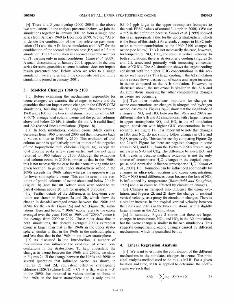
[7] We consider here GEOS CCM [Pawson et al., 2008]simulations of the past (1960–2004) and future (2000–2100). The past simulations use the observed Hadley seasurface temperatures (SSTs) and sea ice data set from Rayneret al. [2003], whereas the future simulations use SSTsand sea ice output from AR4 integrations of the NationalCenter for Atmospheric Research Community ClimateSystemModel, Version 3 for both the IPCC [2001]A1b andA2GHG scenarios. Observed surface concentrations of GHGsand halogens are used for past simulations. Future simulationsuse the A1b or A2 scenario for surface concentrations ofGHGs and the WMO [2003] Ab scenario for surface con-centrations of halogens. The time series of the surface con-centrations of the GHGs and total chlorine, normalized bytheir 1960 values, are shown in Figure 1a. The two GHGscenarios are fairly similar until about 2040, when theA2 scenario shows faster increases of CO2 and N2O. CH4

continues to increase in this scenario whereas it peaksaround 2050 in the A1b scenario.[8] Comparisons of the simulated temperature, ozone,

water vapor, and other constituents with observations havebeen discussed by Pawson et al. [2008], Eyring et al. [2006,2007], and Oman et al. [2008]. These studies have shownthat GEOS CCM performs reasonably well compared toobservations. Two noted deficiencies are a high bias in totalO3 at high latitudes when chlorine loading is low (in the1960s) and the late breakup of the Antarctic polar vortex[Pawson et al., 2008].

Figure 1. Temporal variation of (a) surface GHGs andhalogens (solid line, A1b; dashed line, A2) and (b) totalor partial column ozone averaged between 60°S and 60°N(solid line, A1b; dashed line, A2), between 1960 and 2100.

OMAN ET AL.: UPPER STRATOSPHERIC OZONE D05303D05303

2 of 13

[9] There is a 5 year overlap (2000–2004) in the abovetwo simulations. In the analysis presented below, we join thesimulations together in January 2001 to form a single timeseries from January 1960 to December 2099. We use “A1b”to denote the combination of the first reference past simu-lation (P1) and the A1b future simulation and “A2” for thecombination of the second reference past (P2) and A2 futuresimulation. The P2 simulation is a second ensemble memberof P1, varying only in initial conditions [Oman et al., 2009].A small discontinuity at January 2001, apparent in the timeseries for some quantities at some locations, does not impactresults presented here. Below when we refer to a singlesimulation, we are referring to the composite past and futuresimulations joined in January 2001.

3. Modeled Changes 1960 to 2100

[10] Before examining the mechanisms responsible forozone changes, we examine the changes in ozone and thequantities that can impact ozone changes in the GEOS CCMsimulations, focusing on the long‐term changes between1960 and 2100 for the two simulations. Evolution of the 60°S–60°N average total column ozone and the partial columnsabove and below 20 hPa is similar for the A1b (solid lines)and A2 (dashed lines) simulations (Figure 1b).[11] In both simulations, column ozone (black curves)

decreases from 1960 to around 2000 and then increases backto values similar to 1960 by 2100. This evolution of totalcolumn ozone is qualitatively similar to that of the negativeof the tropospheric total chlorine (Figure 1a), except thetotal chlorine peaks a few years earlier and has not quitereturned to 1960 values by 2100. Although the extrapolartotal column ozone in 2100 is similar to that in the 1960s,this is not necessarily the case for the ozone mixing ratio at agiven location. In general, upper stratospheric ozone in the2090s exceeds the 1960s values whereas the opposite is truefor lower stratospheric ozone. This can be seen in the evo-lution of partial columns of ozone above and below 20 hPa(Figure 1b) (note that 80 Dobson units were added to thepartial column above 20 hPa for graphical purposes).[12] Further details of the differences in long‐term evo-

lution are shown in Figures 2a and 2b, which show thechange in decadal‐averaged ozone between the 1960s and2090s for the ‐A1b (Figure 2a) and A2 (Figure 2b) simu-lations. Here and below, “1960s” ozone refers to the ozoneaveraged over the years 1960 to 1969, and “2090s” ozone isthe average from 2090 to 2099. These plots show that inboth simulations, the decadal‐averaged 2090s extrapolarozone is larger than that in the 1960s in the upper strato-sphere, similar to that in the 1960s in the midstratosphere,and less than that in the 1960s in the lower stratosphere.[13] As discussed in the Introduction, a number of

mechanisms can influence the evolution of ozone con-centrations in the stratosphere. To help understand thechanges in ozone between the 1960s and 2090s, we showin Figures 2c–2l the change between the 1960s and 2090s inseveral quantities that influence ozone. As shown inFigures 2c and 2d, equivalent effective stratosphericchlorine (EESC) (where EESC = Cly + a Bry, with a = 5)in the 2090s has returned to values similar to those inthe 1960s in the lower stratosphere and is only around

0.3–0.5 ppb larger in the upper stratosphere (compare tothe peak EESC values of around 3–4 ppb in 2000). (We usea = 5 in the definition because Daniel et al. [1999] showedthis is an appropriate value for the upper stratosphere, whichis the focus of this study.) As a result, changes in EESC onlymake a minor contribution to the 1960–2100 changes inozone (see below). This is not necessarily the case, however,for temperature, NOy, HOx, and residual vertical velocity. Inboth simulations, there is stratospheric cooling (Figures 2eand 2f), associated primarily with increasing concentra-tions of GHGs. The A2 simulation shows the largest coolingconsistent with the higher GHG concentrations in this sce-nario (see Figure 1a). This larger cooling in the A2 simulationalone causes slower destruction of ozone and larger increasesin ozone compared to the A1b simulation. However, asdiscussed above, the net ozone is similar in the A1b andA2 simulations, implying that other compensating changesin ozone are occurring.[14] Two other mechanisms important for changes in

ozone concentrations are changes in nitrogen and hydrogenozone‐loss cycles. Figures 2g–2j show that the magnitude ofchanges in NOy and HOx between the 1960s and 2090s aredifferent in the A1b andA2 simulations, with a larger increasein upper stratospheric NOy and HOx in the A2 simulation(again, consistent with higher GHG concentrations in thisscenario; see Figure 1a). It is important to note that changesin HOx and NOy do not simply follow changes in CH4 andN2O, respectively. This can be seen by comparing Figures 2gand 2i with Figure 1a: there are negative changes in someareas in NOy and HOx from the 1960s to 2090s despite largeincreases in N2O and CH4. The difference between HOx andCH4 trends is because methane oxidation is not the onlysource of stratospheric H2O; changes in the tropical tropo-pause cold point also influence stratospheric H2O [Oman etal., 2008]. HOx formation can be influenced additionally bychanges in ultraviolet radiation and ozone concentration.NOy − N2O trend differences occur because the loss of NOy

is influenced by temperature [Rosenfield and Douglass,1998] and also could be affected by circulation changes.[15] Changes in transport also influence the ozone evo-

lution, and Figures 2k and 2l show the change in residualvertical velocity, as a proxy for circulation changes. There isa similar increase in the tropical vertical velocity betweenthe 1960s and 2090s in the two simulations, with a slightlylarger change in the A2 simulation.[16] In summary, Figure 2 shows that there are larger

changes in temperature, NOy, and HOx in the A2 simulation,but the ozone change is similar in the two simulations. Thissuggests compensating ozone changes caused by differentmechanisms, which is quantified below.

4. Linear Regression Analysis

[17] We want to estimate the contribution of the differentmechanisms to the simulated changes in ozone. The prin-cipal analysis method used to do this is MLR. For a givenlocation and time, MLR is applied to determine the coeffi-cients mX such that

�O3 tð Þ ¼X

j

mXj�Xj tð Þ þ " tð Þ; ð1Þ


3 of 13

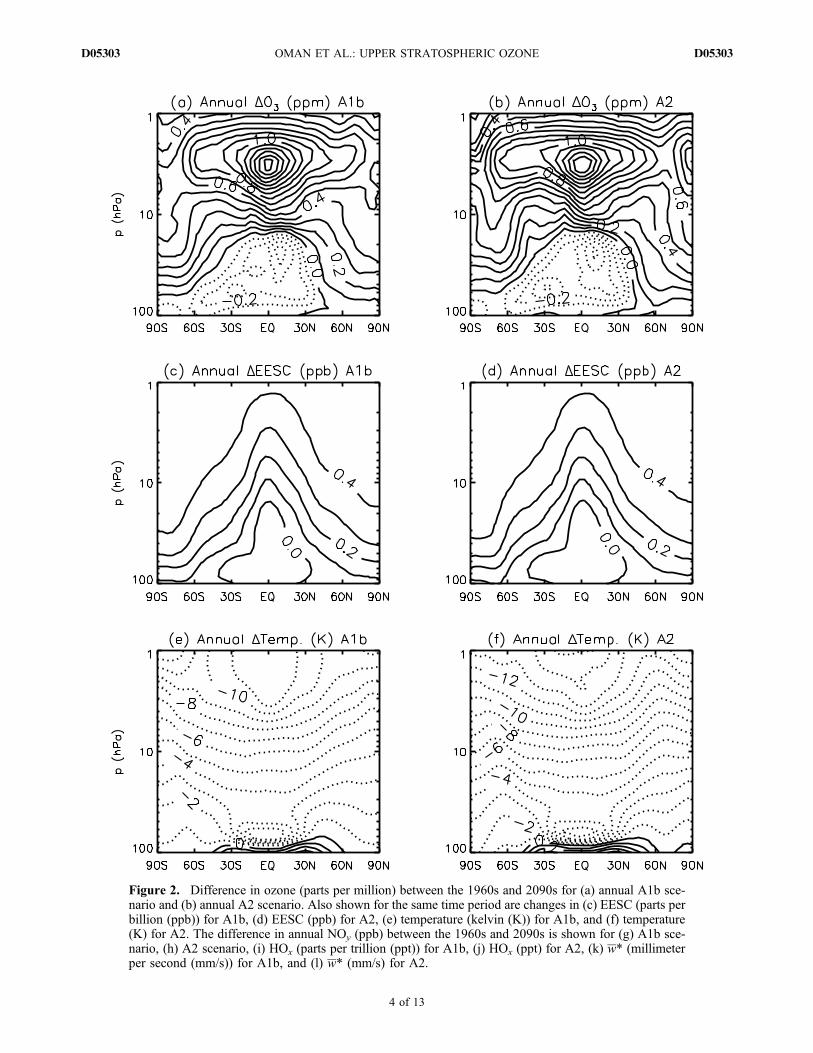
Figure 2. Difference in ozone (parts per million) between the 1960s and 2090s for (a) annual A1b sce-nario and (b) annual A2 scenario. Also shown for the same time period are changes in (c) EESC (parts perbillion (ppb)) for A1b, (d) EESC (ppb) for A2, (e) temperature (kelvin (K)) for A1b, and (f) temperature(K) for A2. The difference in annual NOy (ppb) between the 1960s and 2090s is shown for (g) A1b sce-nario, (h) A2 scenario, (i) HOx (parts per trillion (ppt)) for A1b, (j) HOx (ppt) for A2, (k) w* (millimeterper second (mm/s)) for A1b, and (l) w* (mm/s) for A2.


4 of 13

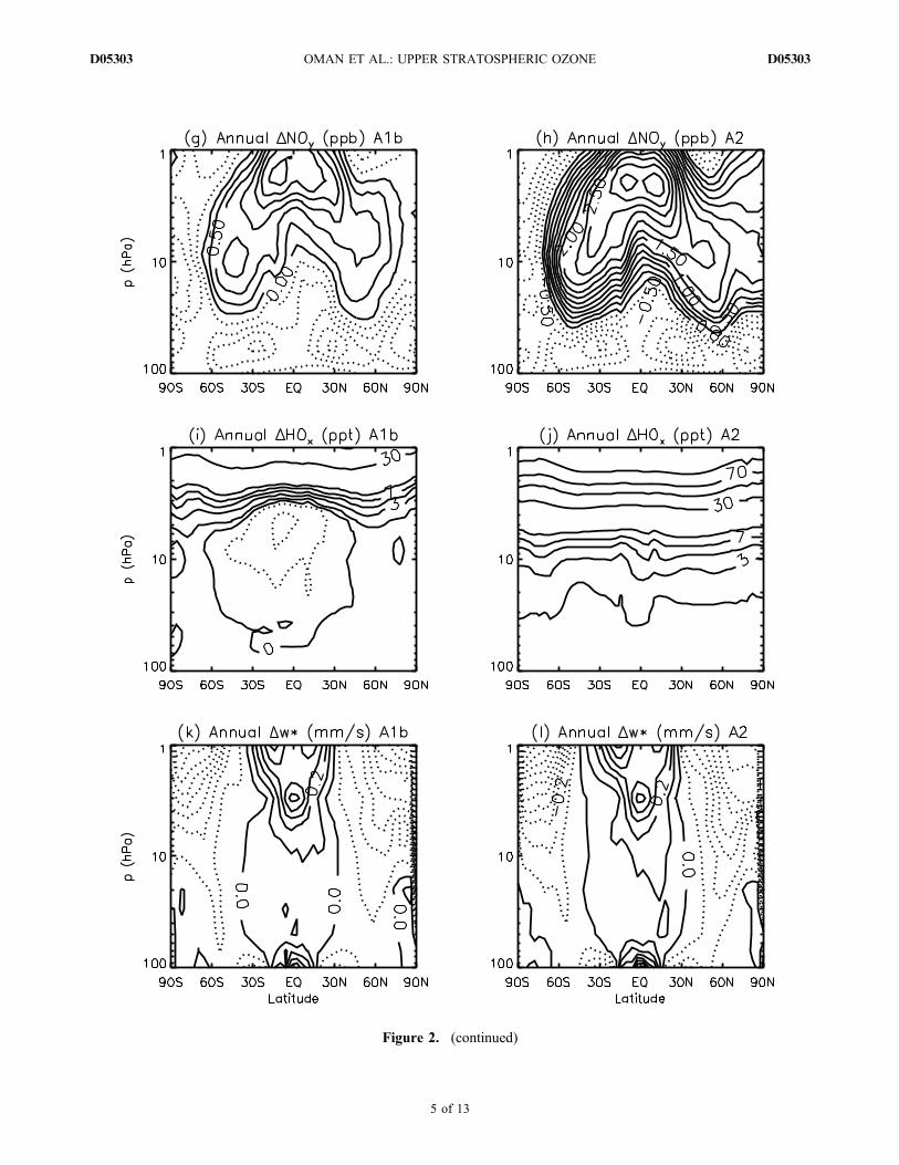
Figure 2. (continued)


5 of 13

where the Xj are the different quantities that could influenceozone, the coefficients mX are the sensitivity of ozone to thequantity X, i.e., mX = ∂O3/∂X, and " is the error in the fit.MLR analysis has been applied extensively to observationsor simulations to isolate a long‐term linear trend in ozone(and, more recently, long‐term variations in ozone corre-lated with EESC) [e.g.,WMO, 2007, and references therein].[18] To apply equation (1), we need to decide which

mechanisms we want to isolate and the quantities Xj that arethe “proxies” for these different mechanisms. In the MLRcalculations presented below, we focus on ozone changescaused by changes in halogen, nitrogen, and hydrogenozone‐loss cycles as well as changes in temperature. To dothis, four explanatory variables (Xj) are used in equation (1):EESC, reactive nitrogen (NOy = NO + NO2 + NO3 + 2*(N2O5) + HNO3 + HO2NO2 + ClONO2 + BrONO2), reac-tive hydrogen (HOx = OH + HO2), and temperature (T ).Each term on the right‐hand side of equation (1) then givesthe “contribution” of the response in ozone due to a changein X and the role the corresponding mechanism plays in theozone evolution (i.e., mEESCDEESC is the contribution dueto changes in EESC and the role of changes in halogenozone‐loss cycles). We chose HOx as an explanatory vari-able rather than H2O, even though it is a shorter‐livedspecies, to address feedbacks that are discussed in section 6that would not be seen using H2O.[19] Rather than using the above four quantities as

explanatory variables X in the MLR analysis, an alternativeapproach would be to use the surface concentrations of theODSs and GHGs as the independent variables X. Stolarski etal. [2010] used this approach when examining temperaturechanges in the GEOS CCM simulations considered here.Also, Shepherd and Jonsson [2008] used ODSs and CO2 toseparate their impact on temperature and ozone changes butcould not quantify the impact of other GHGs, although theyare likely to have a smaller impact. However, as discussedabove, changes in HOx and NOy do not simply followchanges in CH4 and N2O, respectively, and regressingagainst CH4 and N2O will not necessarily isolate the role ofchanges in the hydrogen and nitrogen cycles in the responseof ozone. Furthermore, the time series of CO2 and N2O arenot independent in terms of correlation for either scenario,and neither are CO2 andCH4 for theA2 scenario (see Figure 1).This means that the MLR could not separate the impact ofthese fields.[20] The model output used in the MLR analysis is from

instantaneous output from the first day of each month sincenot all variables were saved as monthly averages; however,using monthly mean data should not materially affect theresults. This analysis was done for individual months as wellas annual averages. Here we focus on presenting resultscalculated using annual averages. Thus, we examine inter-annual and longer time scale variations in ozone. The aboveMLR analysis presented below uses all 140 years of theGEOS CCM simulations to determine the coefficients mX.Calculations using shorter time periods (i.e., different startor end dates) show some sensitivity to the period used (e.g.,if the start date is between 1960 and 1990 and the end date isbetween 2050 and 2100, there is some variation in thecoefficients).[21] There are several complications with the above linear

regression approach. First, other mechanisms that are not

considered in the regression (e.g., transport) could play arole. Second, significant correlations can exist between thetemporal variations of the quantities, i.e., the quantities arenot necessarily independent. Third, a high correlationbetween ozone and a quantity does not show causality, asozone could be causing the quantity to change, or changes inanother quantity could be causing both ozone and thequantity of interest to change in a correlated way. Temper-ature and ozone in the upper stratosphere is an example ofthis third complication: changes in ozone cause, throughchanges in short‐wave heating, changes in temperature. Atthe same time, changes in temperature cause, throughchanges in reaction rates, differences in the response ofozone. Also, the relationship between the variables we useand ozone may not be linear. Because of the above com-plications, caution must be applied when interpreting theMLR results presented below. Additional discussion andanalysis of these issues is included below.

5. Relative Contributions to Ozone Changes

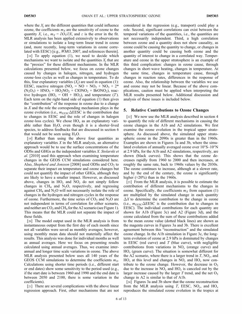
[22] We now use the MLR analysis described in section 4to quantify the role of different mechanisms in causing theozone changes in the A1b and A2 simulations. We firstexamine the ozone evolution in the tropical upper strato-sphere. As discussed above, the simulated upper strato-spheric ozone in the 2090s is greater than in the 1960s.Examples are shown in Figures 3a and 3b, where the simu-lated evolution of annually averaged ozone over 10°S–10°Nat 2.9 hPa, for the A1b and A2 simulations, respectively, areshown (black curves). This shows that the ozone de-creases rapidly from 1960 to 2000 and then increases, atroughly the same rate, back to 1960s values by the 2030s.The ozone continues to increase, although at a slower rate,and by the end of the century, the ozone is significantlyhigher (≈20%) than in the 1960s.[23] From the MLR analysis, it is possible to estimate the

contribution of different mechanisms to the changes inozone. Specifically, the coefficients mX from equation (1)are multiplied by the simulated change in each quantityDX to determine the contribution to the change in ozone(i.e., mEESCDEESC is the contribution due to changes inEESC). The individual contributions for each quantity areshown for A1b (Figure 3c) and A2 (Figure 3d), and theozone calculated from the sum of these contributions addedto the mean ozone value (dotted black lines) are shown asthe magenta curves in Figures 3a and 3b. There is excellentagreement between this “reconstruction” and the simulatedozone change. In the A1b simulation in Figure 3c, the long‐term evolution of ozone at 2.9 hPa is dominated by changesin EESC (red curve) and T (blue curve), with negligiblecontributions from variations in NOy (orange curve) andHOx (green curve). The situation is somewhat different forthe A2 scenario, where there is a larger trend in T, NOy, andHOx at this level and changes in NOy and HOx now con-tribute to the ozone change. However, the decrease in O3

due to the increase in NOy and HOx is canceled out by thelarger increase caused by the larger T trend, and the net O3

change in A2 is similar to that of A1b.[24] Figures 3a and 3b show that the ozone reconstruction

from the MLR analysis using T, EESC, NOy, and HOx

reproduces the simulated ozone evolution in the tropics at


6 of 13

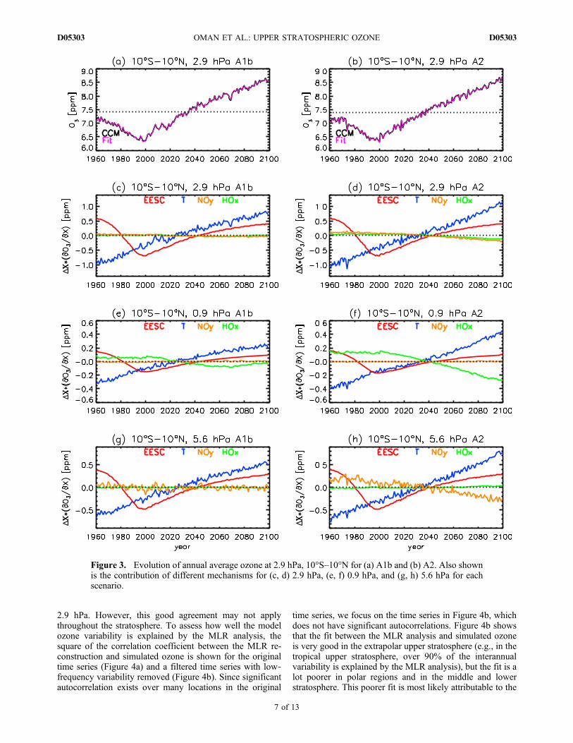
2.9 hPa. However, this good agreement may not applythroughout the stratosphere. To assess how well the modelozone variability is explained by the MLR analysis, thesquare of the correlation coefficient between the MLR re-construction and simulated ozone is shown for the originaltime series (Figure 4a) and a filtered time series with low‐frequency variability removed (Figure 4b). Since significantautocorrelation exists over many locations in the original

time series, we focus on the time series in Figure 4b, whichdoes not have significant autocorrelations. Figure 4b showsthat the fit between the MLR analysis and simulated ozoneis very good in the extrapolar upper stratosphere (e.g., in thetropical upper stratosphere, over 90% of the interannualvariability is explained by the MLR analysis), but the fit is alot poorer in polar regions and in the middle and lowerstratosphere. This poorer fit is most likely attributable to the

Figure 3. Evolution of annual average ozone at 2.9 hPa, 10°S–10°N for (a) A1b and (b) A2. Also shownis the contribution of different mechanisms for (c, d) 2.9 hPa, (e, f) 0.9 hPa, and (g, h) 5.6 hPa for eachscenario.


7 of 13

larger role of transport, which is not explicitly accounted forin the MLR analysis. Because of the above, we focus ourMLR analysis on ozone changes in the extrapolar upperstratosphere.[25] The analysis at 2.9 hPa indicates that changes in NOy

and HOx make negligible contributions to ozone changes forthe A1b simulation, but NOy and HOx do make significantcontributions for the A2 simulation. However, the con-tributions of the different quantities vary with altitude. Thisis illustrated in Figures 3e–3h, which show the contributionsfor 0.9 and 5.6 hPa. (The simulated ozone and MLR re-construction are not shown as the evolution and agreementis similar to that for 2.9 hPa.) At 0.9 hPa (Figures 3e and 3f),HOx‐related ozone loss is more important than at 2.9 hPa.This is especially evident in the A2 scenario (Figure 3f) inwhich there is a much larger CH4 trend yielding a largerHOx trend. The larger HOx‐related ozone loss is again offsetby larger T contributions. In contrast to 0.9 hPa, NOy‐relatedozone loss is important at 5.6 hPa for the A2 scenario(Figure 3h). In the A1b simulation, NOy variations con-tribute to year‐to‐year variability but not to the long‐termtrend (Figure 3g), whereas in the A2 simulation, variationsin NOy contribute to the long‐term behavior (Figure 3h).The trend caused by increased NOy results in an ozonedecrease of 0.5 ppm from the 1960s to the 2090s. As withthe larger changes in T and HOx at 0.9 hPa, the largerchanges in T and NOy in the A2 simulation at 5.6 hPa causelarger changes in ozone, but these changes are of oppositesign, and the net change in ozone in A2 is similar to that inthe A1b simulation.

[26] Close inspection of Figures 3c–3h shows the relativecontributions of the different mechanisms to changes inozone vary with time. This is quantified in Figure 5, whichshows the vertical variation of the changes in tropical ozoneand individual contributions of different mechanisms for theA1b (solid curves) and A2 (dashed curves) simulations, over1960–2000 (Figure 5a), 2000–2100 (Figure 5b), and 1960–2100 (Figure 5c).

Figure 4. Annual correlation coefficient squared for (a) theoriginal model ozone time series and MLR fit and (b) a fil-tered time series with low‐frequency variability removed byapplying a 1:2:1 filter iteratively 30 times to each quantity.

Figure 5. Vertical variation of changes in ozone (solid blackcurve) and individual contribution of different mechanismsfor annual averages over the tropics. The changes are for(a) 1990s minus 1960s P1 (solid curve) and P2 (dashed curve),(b) 2090sminus 2000sA1b (solid curve) forA2 (dashed curve)scenario, and (c) 2090s minus 1960s A1b (solid curve) forA2 (dashed curve) scenario.


8 of 13

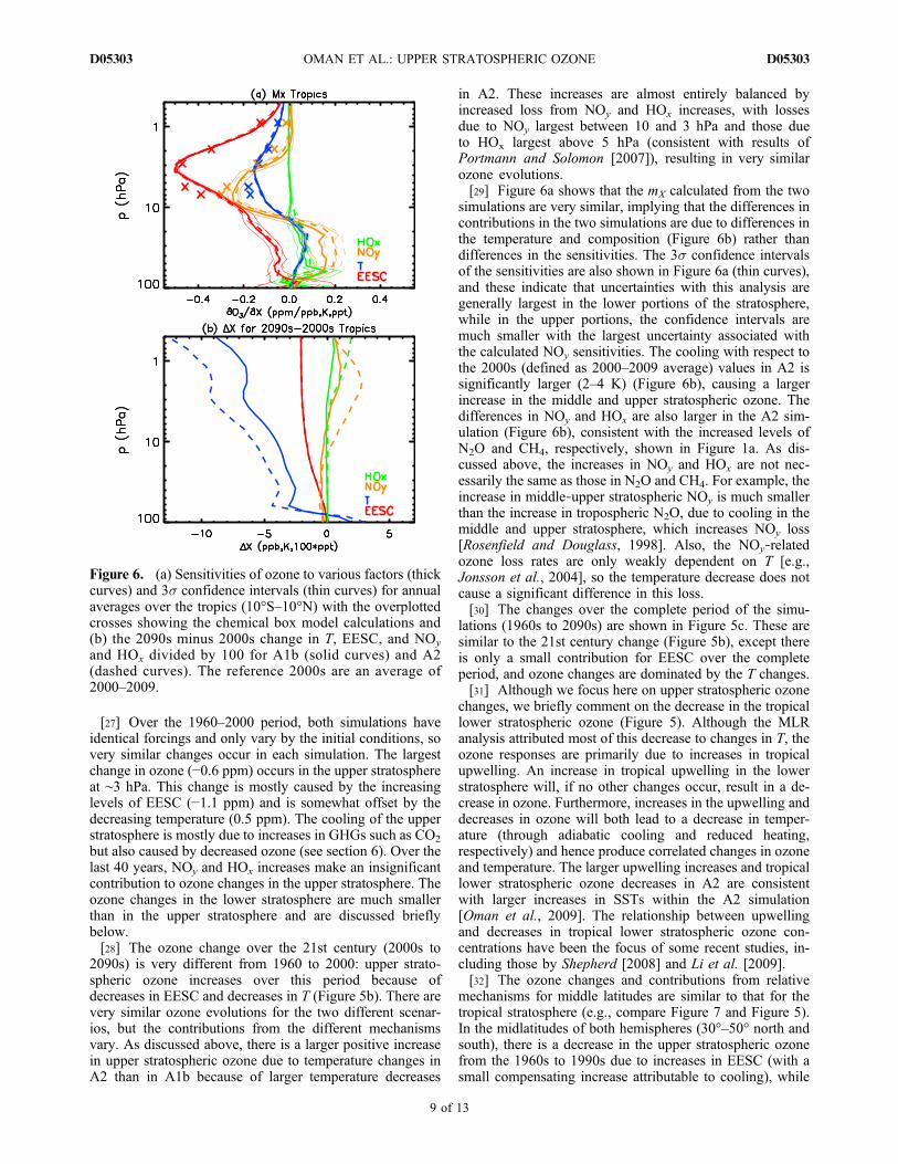
[27] Over the 1960–2000 period, both simulations haveidentical forcings and only vary by the initial conditions, sovery similar changes occur in each simulation. The largestchange in ozone (−0.6 ppm) occurs in the upper stratosphereat ∼3 hPa. This change is mostly caused by the increasinglevels of EESC (−1.1 ppm) and is somewhat offset by thedecreasing temperature (0.5 ppm). The cooling of the upperstratosphere is mostly due to increases in GHGs such as CO2

but also caused by decreased ozone (see section 6). Over thelast 40 years, NOy and HOx increases make an insignificantcontribution to ozone changes in the upper stratosphere. Theozone changes in the lower stratosphere are much smallerthan in the upper stratosphere and are discussed brieflybelow.[28] The ozone change over the 21st century (2000s to

2090s) is very different from 1960 to 2000: upper strato-spheric ozone increases over this period because ofdecreases in EESC and decreases in T (Figure 5b). There arevery similar ozone evolutions for the two different scenar-ios, but the contributions from the different mechanismsvary. As discussed above, there is a larger positive increasein upper stratospheric ozone due to temperature changes inA2 than in A1b because of larger temperature decreases

in A2. These increases are almost entirely balanced byincreased loss from NOy and HOx increases, with lossesdue to NOy largest between 10 and 3 hPa and those dueto HOx largest above 5 hPa (consistent with results ofPortmann and Solomon [2007]), resulting in very similarozone evolutions.[29] Figure 6a shows that the mX calculated from the two

simulations are very similar, implying that the differences incontributions in the two simulations are due to differences inthe temperature and composition (Figure 6b) rather thandifferences in the sensitivities. The 3s confidence intervalsof the sensitivities are also shown in Figure 6a (thin curves),and these indicate that uncertainties with this analysis aregenerally largest in the lower portions of the stratosphere,while in the upper portions, the confidence intervals aremuch smaller with the largest uncertainty associated withthe calculated NOy sensitivities. The cooling with respect tothe 2000s (defined as 2000–2009 average) values in A2 issignificantly larger (2–4 K) (Figure 6b), causing a largerincrease in the middle and upper stratospheric ozone. Thedifferences in NOy and HOx are also larger in the A2 sim-ulation (Figure 6b), consistent with the increased levels ofN2O and CH4, respectively, shown in Figure 1a. As dis-cussed above, the increases in NOy and HOx are not nec-essarily the same as those in N2O and CH4. For example, theincrease in middle‐upper stratospheric NOy is much smallerthan the increase in tropospheric N2O, due to cooling in themiddle and upper stratosphere, which increases NOy loss[Rosenfield and Douglass, 1998]. Also, the NOy‐relatedozone loss rates are only weakly dependent on T [e.g.,Jonsson et al., 2004], so the temperature decrease does notcause a significant difference in this loss.[30] The changes over the complete period of the simu-

lations (1960s to 2090s) are shown in Figure 5c. These aresimilar to the 21st century change (Figure 5b), except thereis only a small contribution for EESC over the completeperiod, and ozone changes are dominated by the T changes.[31] Although we focus here on upper stratospheric ozone

changes, we briefly comment on the decrease in the tropicallower stratospheric ozone (Figure 5). Although the MLRanalysis attributed most of this decrease to changes in T, theozone responses are primarily due to increases in tropicalupwelling. An increase in tropical upwelling in the lowerstratosphere will, if no other changes occur, result in a de-crease in ozone. Furthermore, increases in the upwelling anddecreases in ozone will both lead to a decrease in temper-ature (through adiabatic cooling and reduced heating,respectively) and hence produce correlated changes in ozoneand temperature. The larger upwelling increases and tropicallower stratospheric ozone decreases in A2 are consistentwith larger increases in SSTs within the A2 simulation[Oman et al., 2009]. The relationship between upwellingand decreases in tropical lower stratospheric ozone con-centrations have been the focus of some recent studies, in-cluding those by Shepherd [2008] and Li et al. [2009].[32] The ozone changes and contributions from relative

mechanisms for middle latitudes are similar to that for thetropical stratosphere (e.g., compare Figure 7 and Figure 5).In the midlatitudes of both hemispheres (30°–50° north andsouth), there is a decrease in the upper stratospheric ozonefrom the 1960s to 1990s due to increases in EESC (with asmall compensating increase attributable to cooling), while

Figure 6. (a) Sensitivities of ozone to various factors (thickcurves) and 3s confidence intervals (thin curves) for annualaverages over the tropics (10°S–10°N) with the overplottedcrosses showing the chemical box model calculations and(b) the 2090s minus 2000s change in T, EESC, and NOy

and HOx divided by 100 for A1b (solid curves) and A2(dashed curves). The reference 2000s are an average of2000–2009.


9 of 13

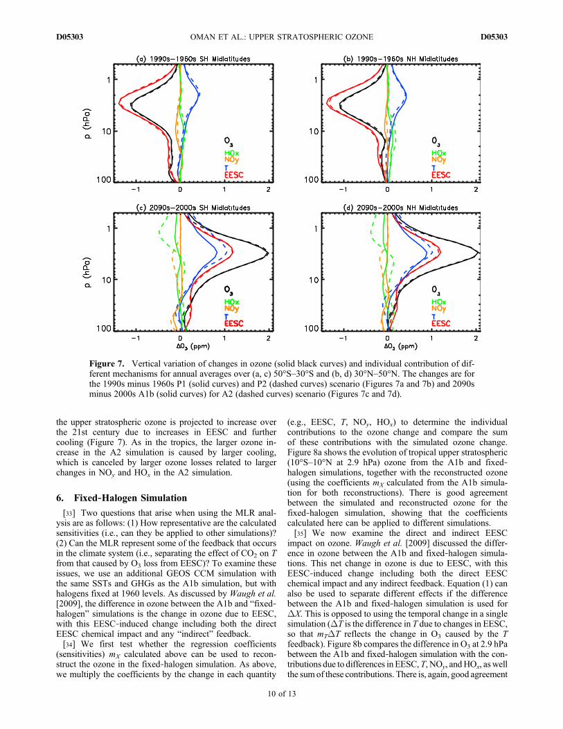
the upper stratospheric ozone is projected to increase overthe 21st century due to increases in EESC and furthercooling (Figure 7). As in the tropics, the larger ozone in-crease in the A2 simulation is caused by larger cooling,which is canceled by larger ozone losses related to largerchanges in NOy and HOx in the A2 simulation.

6. Fixed‐Halogen Simulation

[33] Two questions that arise when using the MLR anal-ysis are as follows: (1) How representative are the calculatedsensitivities (i.e., can they be applied to other simulations)?(2) Can the MLR represent some of the feedback that occursin the climate system (i.e., separating the effect of CO2 on Tfrom that caused by O3 loss from EESC)? To examine theseissues, we use an additional GEOS CCM simulation withthe same SSTs and GHGs as the A1b simulation, but withhalogens fixed at 1960 levels. As discussed by Waugh et al.[2009], the difference in ozone between the A1b and “fixed‐halogen” simulations is the change in ozone due to EESC,with this EESC‐induced change including both the directEESC chemical impact and any “indirect” feedback.[34] We first test whether the regression coefficients

(sensitivities) mX calculated above can be used to recon-struct the ozone in the fixed‐halogen simulation. As above,we multiply the coefficients by the change in each quantity

(e.g., EESC, T, NOy, HOx) to determine the individualcontributions to the ozone change and compare the sumof these contributions with the simulated ozone change.Figure 8a shows the evolution of tropical upper stratospheric(10°S–10°N at 2.9 hPa) ozone from the A1b and fixed‐halogen simulations, together with the reconstructed ozone(using the coefficients mX calculated from the A1b simula-tion for both reconstructions). There is good agreementbetween the simulated and reconstructed ozone for thefixed‐halogen simulation, showing that the coefficientscalculated here can be applied to different simulations.[35] We now examine the direct and indirect EESC

impact on ozone. Waugh et al. [2009] discussed the differ-ence in ozone between the A1b and fixed‐halogen simula-tions. This net change in ozone is due to EESC, with thisEESC‐induced change including both the direct EESCchemical impact and any indirect feedback. Equation (1) canalso be used to separate different effects if the differencebetween the A1b and fixed‐halogen simulation is used forDX. This is opposed to using the temporal change in a singlesimulation (DT is the difference in T due to changes in EESC,so that mTDT reflects the change in O3 caused by the Tfeedback). Figure 8b compares the difference in O3 at 2.9 hPabetween the A1b and fixed‐halogen simulation with the con-tributions due to differences inEESC,T, NOy, andHOx, aswellthe sum of these contributions. There is, again, good agreement

Figure 7. Vertical variation of changes in ozone (solid black curves) and individual contribution of dif-ferent mechanisms for annual averages over (a, c) 50°S–30°S and (b, d) 30°N–50°N. The changes are forthe 1990s minus 1960s P1 (solid curves) and P2 (dashed curves) scenario (Figures 7a and 7b) and 2090sminus 2000s A1b (solid curves) for A2 (dashed curves) scenario (Figures 7c and 7d).


10 of 13

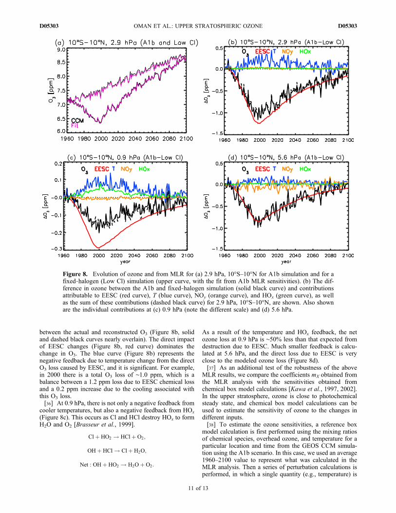
between the actual and reconstructed O3 (Figure 8b, solidand dashed black curves nearly overlain). The direct impactof EESC changes (Figure 8b, red curve) dominates thechange in O3. The blue curve (Figure 8b) represents thenegative feedback due to temperature change from the directO3 loss caused by EESC, and it is significant. For example,in 2000 there is a total O3 loss of ∼1.0 ppm, which is abalance between a 1.2 ppm loss due to EESC chemical lossand a 0.2 ppm increase due to the cooling associated withthis O3 loss.[36] At 0.9 hPa, there is not only a negative feedback from

cooler temperatures, but also a negative feedback from HOx

(Figure 8c). This occurs as Cl and HCl destroy HOx to formH2O and O2 [Brasseur et al., 1999].

Clþ HO2 ! HClþ O2;

OHþ HCl ! Clþ H2O;

Net : OHþ HO2 ! H2Oþ O2:

As a result of the temperature and HOx feedback, the netozone loss at 0.9 hPa is ∼50% less than that expected fromdestruction due to EESC. Much smaller feedback is calcu-lated at 5.6 hPa, and the direct loss due to EESC is veryclose to the modeled ozone loss (Figure 8d).[37] As an additional test of the robustness of the above

MLR results, we compare the coefficients mX obtained fromthe MLR analysis with the sensitivities obtained fromchemical box model calculations [Kawa et al., 1997, 2002].In the upper stratosphere, ozone is close to photochemicalsteady state, and chemical box model calculations can beused to estimate the sensitivity of ozone to the changes indifferent inputs.[38] To estimate the ozone sensitivities, a reference box

model calculation is first performed using the mixing ratiosof chemical species, overhead ozone, and temperature for aparticular location and time from the GEOS CCM simula-tion using the A1b scenario. In this case, we used an average1960–2100 value to represent what was calculated in theMLR analysis. Then a series of perturbation calculations isperformed, in which a single quantity (e.g., temperature) is

Figure 8. Evolution of ozone and from MLR for (a) 2.9 hPa, 10°S–10°N for A1b simulation and for afixed‐halogen (Low Cl) simulation (upper curve, with the fit from A1b MLR sensitivities). (b) The dif-ference in ozone between the A1b and fixed‐halogen simulation (solid black curve) and contributionsattributable to EESC (red curve), T (blue curve), NOy (orange curve), and HOx (green curve), as wellas the sum of these contributions (dashed black curve) for 2.9 hPa, 10°S–10°N, are shown. Also shownare the individual contributions at (c) 0.9 hPa (note the different scale) and (d) 5.6 hPa.


11 of 13

increased and decreased from its reference value. For EESC,Cly was perturbed ±0.1 ppb, and Bry was perturbed ±1 ppt;temperature was perturbed ±5 K; and NOy was perturbed±1 ppb. Each simulation was run for 20 days, by which timethe solution has closely approached steady state. The re-sulting change in ozone gives an estimate of the sensitivityof ozone to changes in this quantity, e.g., DO3/DX providesan estimate of sensitivity of ozone to changes in variable X.This sensitivity can then be directly compared with thecoefficients mX from equation (1).[39] Figure 6a shows the variation in calculated steady

state ozone to changes in T, EESC, and NOy (coloredcrosses) for reference calculations based on simulated fieldsat several levels between 6.9 and 0.9 hPa for July at 2°N.Although we use annual average values for the MLR anal-ysis, tests using other months in the chemical box modelproduced only small changes. These values are generally invery good agreement with the coefficients from the MLRanalysis. Some disagreement is seen at 5.6 and 6.9 hPa withslightly higher EESC, NOy, and T sensitivities from thechemical box. NOy sensitivities are, in general, slightlylarger in the box model than calculated in the MLR analysis.It is not clear, at this point, why there are some differencesseen in the sensitivities between the MLR analysis and thebox model. Even though there is some disagreement, overallthe two methods show a similar picture and give us confi-dence in the MLR‐based attribution of the relative con-tributions of different factors to the changes in ozone.

7. Conclusions

[40] In this study, we have quantified the contribution ofdifferent mechanisms to changes in the upper stratosphericozone from 1960 to 2100 in GEOS CCM simulations andseparated the direct and indirect impacts of EESC on ozone.Simulations using two different GHG scenarios (A1b andA2 from IPCC [2001]) were considered, and even thoughthere are significant differences in the GHG concentrationsin the latter half of the 21st century, there is a very similarincrease in the upper stratospheric ozone over the 21stcentury. Isolation of different mechanisms using MLRshows that the similar ozone evolution is because of com-pensating effects of different mechanisms. In the A1b sce-nario, the increase in ozone is caused by decreases inhalogenated ODSs and cooling, which is largely due toincreased GHGs that alter the kinetics rate of ozonedestruction, with the two mechanisms making roughly equalcontributions to the ozone change. Changes in abundance ofreactive nitrogen and hydrogen play only a minor role inlong‐term changes in the A1b scenario. In contrast, in theA2 simulation, there are significant increases in NOy andHOx that cause a long‐term negative decrease in ozone.These decreases are largely offset by a larger positive con-tribution from cooler temperatures, and the ozone evolutionin A2 ends up being very similar to that in A1b.[41] The MLR analysis, together with a fixed‐halogen

simulation, was also used to separate the direct chemicalimpact and indirect feedback of EESC on ozone. The indi-rect impact and mechanisms were shown to vary with alti-tude. At 5.6 hPa, the indirect impacts are small but makesignificant contributions at 2.9 and 0.9 hPa. At 2.9 hPa,there is a negative feedback due to temperature increases

from the direct O3 loss caused by EESC chemistry. Thisfeedback is around 15% the direct EESC impact. At 0.9 hPa,there is negative feedback from temperature and fromchanges in HOx due to changes in EESC, and the sum ofthese is around 50% of the direct EESC impact.[42] The results presented above are based on simulations

from a single model, and it will be important to considersimulations from other models. Preliminary application ofthe MLR method to A1b simulations from several of theCCMs examined by Eyring et al. [2007] yields very similarresults to those presented here for the GEOS CCM (data notshown). In particular, the sensitivities are very similar, anddifferences in ozone evolution can be related to differencesin simulated EESC, T, and NOy fields. As well as consid-ering other models, it will be important to consider a widerrange of GHG scenarios. The very similar ozone evolutionfor the A1B and A2 GHG scenarios considered here mightlead one to think that the ozone evolution would be similarfor all likely GHG scenarios. However, the similarity be-tween the A1B and A2 scenarios considered here occurs bythe chance cancellation of differences in temperature andnitrogen and hydrogen loss cycles, and this is unlikely to bethe case for all possible scenarios (e.g., for the A1F1 and B1scenarios). It will therefore be important to perform simu-lations with a wider range of GHG scenarios when makingprojections of stratospheric ozone.[43] This analysis of models using MLR raises the pos-

sibility of using MLR analysis to separate the contributionsof changes in EESC and T to observed ozone changes. Onedifficulty with applying this method to data is the avail-ability of simultaneous time series of observed ozone,EESC, T, and other quantities used in the MLR analysis.Another issue is the need to consider time periods overwhich the different quantities have sufficiently differenttemporal variations to be isolated in the MLR analysis. Forthe 140 years of simulation considered here, this is possiblefor EESC and T, but this may not be the case for shorterperiods, and more analyses are needed to determine overwhich period data will be required to perform these analyses.

[44] Acknowledgments. This research was supported by the NASAMAP and NSF Large‐scale Climate Dynamics programs. We thank J. EricNielsen for running the model simulations; Stacey Frith for helping with themodel output processing; and Chang Lang, Qing Liang, and Tak Igusa forhelpful comments. We also thank two anonymous reviewers for helpfulcomments and additions. We also thank those involved in model develop-ment at GSFC and high‐performance computing resources on NASA’s“Project Columbia.”

ReferencesAustin, J., and R. J. Wilson (2006), Ensemble simulations of the declineand recovery of stratospheric ozone, J. Geophys. Res., 111, D16314,doi:10.1029/2005JD006907.

Brasseur, G., and M. H. Hitchman (1988), Stratospheric response to tracegas perturbations: Changes in ozone and temperature distributions,Science, 240, 634–637, doi:10.1126/science.240.4852.634.

Brasseur, G. P., J. J. Orlando, and G. S. Tyndall (1999), AtmosphericChemistry and Global Change, Oxford Univ. Press, Oxford, U. K.

Chipperfield, M. P., and W. Feng (2003), Comment on “Stratosphericozone depletion at northern mid‐latitudes in the 21st century: The impor-tance of future concentrations of greenhouse gases nitrous oxide andmethane ,” Geophys . Res . Le t t . , 30 (7 ) , 1389 , do i :10.1029/2002GL016353.

Daniel, J. S., S. Solomon, R. W. Portmann, and R. R. Garcia (1999), Strato-spheric ozone destruction: The importance of bromine relative to chlo-rine, J. Geophys. Res., 104, 23,871–23,880, doi:10.1029/1999JD900381.


12 of 13

Eyring, V., et al. (2006), Assessment of temperature, trace species, andozone in chemistry‐climate model simulations of the recent past, J. Geo-phys. Res., 111, D22308, doi:10.1029/2006JD007327.

Eyring, V., et al. (2007), Multimodel projections of stratospheric ozone inthe 21st century, J. Geophys. Res., 112, D16303, doi:10.1029/2006JD008332.

Haigh, J. D., and J. A. Pyle (1979), A two‐dimensional calculation includ-ing atmospheric carbon dioxide and stratospheric ozone, Nature, 279,222–224, doi:10.1038/279222a0.

Intergovernmental Panel on Climate Change (IPCC) (2001), Contributionof Working Group I to the Third Assessment Report of the Intergovern-mental Panel on Climate Change (IPCC), 944 pp., Cambridge Univ.Press, Cambridge, U. K.

Jonsson, A. I., et al. (2004), Doubled CO2‐induced cooling in the middleatmosphere: Photochemical analysis of the ozone radiative feedback,J. Geophys. Res., 109, D24103, doi:10.1029/2004JD005093.

Kawa, S. R., et al. (1997), Activation of chlorine in sulfate as inferred fromaircraft observations, J. Geophys. Res., 102, 3921–3933, doi:10.1029/96JD01992.

Kawa, S. R., R. Bevilacqua, J. J. Margitan, A. R. Douglass, M. R. Schoeberl,K. Hoppel, and B. Sen (2002), The interaction between dynamics andchemistry of ozone in the set‐up phase of the Northern Hemisphere polarvortex, J. Geophys. Res., 107(D5), 8310, doi:10.1029/2001JD001527.[Printed 108(D5), 2003.]

Li, F., R. S. Stolarski, and P. A. Newman (2009), Stratospheric ozone in thepost‐CFC era, Atmos. Chem. Phys., 9, 2207–2213.

Newchurch, M. J., E.‐S. Yang, D. M. Cunnold, G. C. Reinsel, J. M.Zawodny, and J. M. Russell III (2003), Evidence for slowdown instratospheric ozone loss: First stage of ozone recovery, J. Geophys.Res., 108(D16), 4507, doi:10.1029/2003JD003471.

Oman, L., D. W. Waugh, S. Pawson, R. S. Stolarski, and J. E. Nielsen(2008), Understanding the changes of stratospheric water vapor in cou-pled chemistry‐climate model simulations, J. Atmos. Sci., 65, 3278–3291, doi:10.1175/2008JAS2696.1.

Oman, L., D. W. Waugh, S. Pawson, R. S. Stolarski, and P. A. Newman(2009), On the influence of anthropogenic forcings on changes in thestratospheric mean age, J. Geophys. Res., 114, D03105, doi:10.1029/2008JD010378.

Pawson, S., R. S. Stolarski, A. R. Douglass, P. A. Newman, J. E. Nielsen,S. M. Frith, and M. L. Gupta (2008), Goddard Earth Observing Systemchemistry‐climate model simulations of stratospheric ozone‐temperaturecoupling between 1950 and 2005, J. Geophys. Res., 113, D12103,doi:10.1029/2007JD009511.

Portmann, R. W., and S. Solomon (2007), Indirect radiative forcing of theozone layer during the 21st century, Geophys. Res. Lett., 34, L02813,doi:10.1029/2006GL028252.

Randeniya, L. K., P. F. Vohralik, and I. C. Plumb (2002), Stratosphericozone depletion at northern mid latitudes in the 21st century: The impor-tance of future concentrations of greenhouse gases nitrous oxide andmethane, Geophys. Res. Lett., 29(4), 1051, doi:10.1029/2001GL014295.

Rayner, N. A., D. E. Parker, E. B. Horton, C. K. Folland, L. V. Alexander,D. P. Rowell, E. C. Kent, and A. Kaplan (2003), Global analyses of seasurface temperature, sea ice, and night marine air temperature since thelate nineteenth century, J. Geophys. Res. , 108(D14), 4407,doi:10.1029/2002JD002670.

Rosenfield, J. E., and A. R. Douglass (1998), Doubled CO2 effects on NOyin a coupled 2‐D model, Geophys. Res. Lett., 25, 4381–4384,doi:10.1029/1998GL900147.

Rosenfield, J. E., A. R. Douglass, and D. B. Considine (2002), The impactof increasing carbon dioxide on ozone recovery, J. Geophys. Res., 107(D6), 4049, doi:10.1029/2001JD000824.

Shepherd, T. G. (2008), Dynamics, stratospheric ozone, and climatechange, Atmos. Ocean, 46, 117–138, doi:10.3137/ao.460106.

Shepherd, T. G., and A. I. Jonsson (2008), On the attribution of stratosphericozone and temperature changes to changes in ozone‐depleting substancesand well‐mixed greenhouse gases, Atmos. Chem. Phys., 8, 1435–1444.

Shindell, D. T., D. Rind, and P. Lonergan (1998), Climate change and themiddle atmosphere. Part IV: Ozone response to doubled CO2, J. Clim.,11, 895–918, doi:10.1175/1520-0442(1998)011<0895:CCATMA>2.0.CO;2.

Stolarski, R. S., A. R. Douglass, P. A. Newman, S. Pawson, and M. R.Schoeberl (2010), Relative contribution of greenhouse gases andozone‐depleting substances to temperature trends in the stratosphere: Achemistry/climate model study, J. Clim., 23, 28–42, doi:10.1175/2009JCLI2955.1.

Waugh, D. W., L. Oman, S. R. Kawa, R. S. Stolarski, S. Pawson, A. R.Douglass, P. A. Newman, and J. E. Nielsen (2009), Impacts of climatechange on stratospheric ozone recovery, Geophys. Res. Lett., 36,L03805, doi:10.1029/2008GL036223.

World Meteorological Organization (WMO) (2003), Scientific assessmentof ozone depletion: 2002, Global Ozone Res. Monit. Proj. Rep. 47,Geneva, Switzerland.

World Meteorological Organization (WMO) (2007), Scientific assessmentof ozone depletion: 2006, Global Ozone Res. Monit. Proj. Rep. 50,Geneva, Switzerland.

A. R. Douglass, S. R. Kawa, P. A. Newman, L. D. Oman, and R. S.Stolarski, Atmospheric Chemistry and Dynamics Branch, NASAGoddard Space Flight Center, Code 613.3, Greenbelt, MD 20771, USA.([email protected])D. W. Waugh, Department of Earth and Planetary Sciences, Johns

Hopkins University, Baltimore, MD 21218, USA.


13 of 13

Documents

Mechanisms and feedback causing changes in upper ... · Mechanisms and feedback causing changes in upper stratospheric ozone in the 21st century ... are shown in Figure 1a