Embed Size (px)
Citation preview

INSTITUTFURMECHANIK
Direct and Inverse Problems in Piezoelectricity
RICAM Miniworkshop, Linz
6.-7. Oct. 2005
Continuum mechanical modeling ofnon-linear ferroelectric material behavior
V. Mehling
Mehling, Linz, 2005 – p.1/33

INSTITUTFURMECHANIK
Outline
Introduction: Phenomenology and Structure of Ferroelectrics
Modeling of ferroelectric material behavior
Modeling through the lengthscales
Micromechanical Models
Thermodynamically consistent modeling
Numerical Examples
Mehling, Linz, 2005 – p.2/33
INSTITUTFURMECHANIK
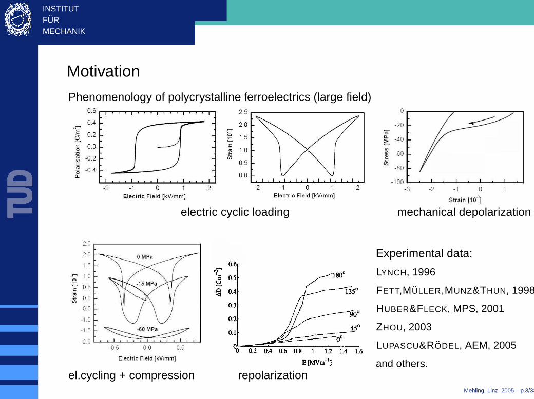
Motivation
Phenomenology of polycrystalline ferroelectrics (large field)
electric cyclic loading mechanical depolarization
Experimental data:
LYNCH, 1996
FETT,MULLER,MUNZ&THUN, 1998
HUBER&FLECK, MPS, 2001
ZHOU, 2003
LUPASCU&RODEL, AEM, 2005
and others.el.cycling + compression repolarization
Mehling, Linz, 2005 – p.3/33

INSTITUTFURMECHANIK
Piezoelectric behavior
coupling of electric/mechanic quantities
direct/inverse piezoelectric effect
’small’ fields – no switching
often considered as linear
reversible, i.e. non-dissipative
Ferroelectric behavior
’large’ fields
switching of unit-cells
non-linear
irreversible, i.e. dissipative
Examples:
tetragonal PZT, BaTiO3
ca
a
c
a
a
aa
a
a
c
a
a
ca
c
a
c
T < Tc
Mehling, Linz, 2005 – p.4/33

INSTITUTFURMECHANIK
Polycrystalline Structure
aa
c
Unit cell Domain
Structure
Polycrystal
Picture: JAFFE ET AL. 1964
Micrograph (BaTi03)
Single crystal grains consist of domains of uniform polarization
Polycrystals constist of multiple grains
The virgin state of the polycrystal
(after cooling below the Curie-Temperature is random and unpolarized)Mehling, Linz, 2005 – p.5/33
INSTITUTFURMECHANIK
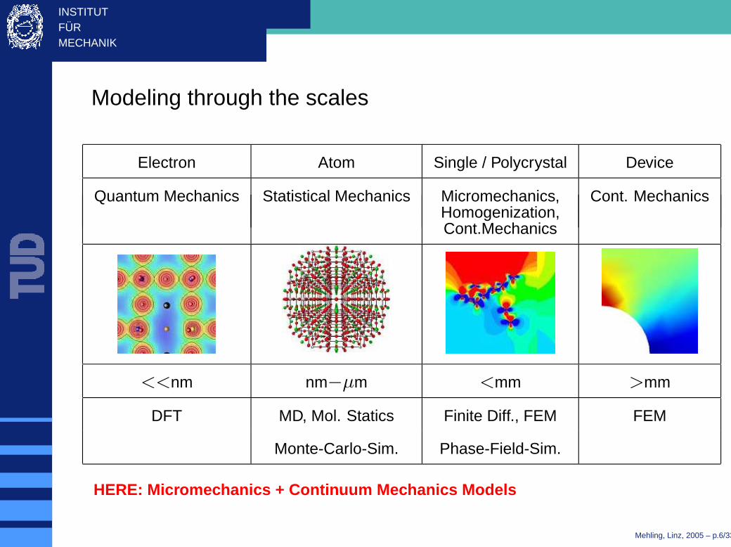
Modeling through the scales
Electron Atom Single / Polycrystal Device
Quantum Mechanics Statistical Mechanics Micromechanics, Cont. MechanicsHomogenization,Cont.Mechanics
<<nm nm−µm <mm >mm
DFT MD, Mol. Statics Finite Diff., FEM FEM
Monte-Carlo-Sim. Phase-Field-Sim.
HERE: Micromechanics + Continuum Mechanics Models
Mehling, Linz, 2005 – p.6/33

INSTITUTFURMECHANIK
Modeling Approaches Literature
Micro-electromechanical approaches:
HWANG,LYNCH&MCMEEKING,1995, CHEN,FANG&HWANG,1997,
HWANG,HUBER,MCMEEKING&FLECK,1998, MICHELITSCH&KREHER,1998,
HWANG&MCMEEKING,1998, LU,FANG,LI,HWANG,1999, KESSLER&BALKE,2001,
HUBER,FLECK,LANDIS,MCMEEKING,1999, WANG,SHI,CHEN,LI, ZHANG, 2005 and others.
Phenomenological modeling approaches:
CHEN 1980, BASSIOUNY,GHALEB&MAUGIN 1988, GHANDI&HAGOOD 1996,
FAN,STOLL&LYNCH 1999, COCKS&MCMEEKING 1999, KAMLAH&JIANG 1999,
KAMLAH&TSAKMAKIS 1999, LANDIS&MCMEEKING 1999, MCMEEKING&LANDIS 1999,
KAMLAH&BOEHLE 2001, LANDIS, JMPS, 2002, KAMLAH&WANG, FZKA, 2003,
LANDIS,WANG,SHENG, JIMSS, 2004, LANDIS, ASME, 2003B and others.
Reviews: KAMLAH 2001, LANDIS 2004.
Mehling, Linz, 2005 – p.7/33

INSTITUTFURMECHANIK Micromechanical Modeling
Single crystal models
Single-crystal – Single-domain: Complete switch
(e.g. HWANG, LYNCH& MCMEEKING 1995, LU, FANG, LI& HWANG 1999)
Single-crystal – Multi-domain: Incremental switching
(e.g. HUBER, FLECK, LANDIS& MCMEEKING 1999)
Phase-field simulations (e.g. WANG,LI,CHEN&ZHANG, 2005)
Phase-field simulation
FEM-mesh
Homogenization
REUSS-assumption: Volume-averaging
(e.g. LU, FANG, LI & HWANG 1999)
Self-consistent scheme
(e.g. HUBER, FLECK, LANDIS & MCMEEKING 1999)
Finite Element Simulations
(e.g. HWANG&MCMEEKING 1998, 1999)
Other homogenization techniques ...
Mehling, Linz, 2005 – p.8/33

INSTITUTFURMECHANIK
Phenomenological modeling
Thermodynamically consistent modeling
Thermodynamic and Electrostatic Balances
Assumptions and Simplifications
Modeling Reversible Processes: Piezoelectricity, Electrostriction
Modeling Irreversible Processes: Internal Variables
Three Examples of Models for Ferroelectricity
Other approachesThere are models, wich are not based on the 2nd law of thermodynamics
e.g. models based on loading and saturation conditions (see Presentation by Marc Kamlah)
e.g. KAMLAH&TSAKMAKIS 1999, KAMLAH&BOHLE 2001
Mehling, Linz, 2005 – p.9/33

INSTITUTFURMECHANIK
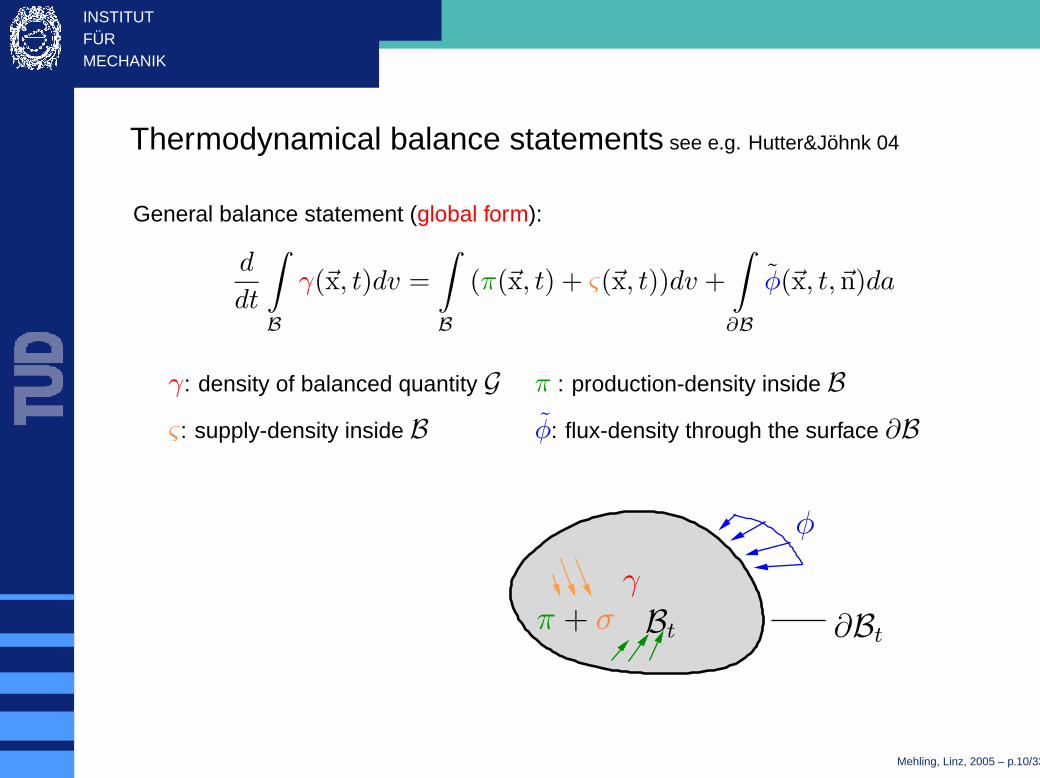
Thermodynamical balance statements see e.g. Hutter&Johnk 04
General balance statement for material body B (global form):
d
dtG = P + S + F
G: balanced quantity P : production inside B
S : supply inside B F : flux through the surface ∂B
∂Bt
F
P + S
Bt
G
Mehling, Linz, 2005 – p.10/33
INSTITUTFURMECHANIK
Thermodynamical balance statements see e.g. Hutter&Johnk 04
General balance statement (global form):
d
dt
∫
B
γ(~x, t)dv =
∫
B
(π(~x, t) + ς(~x, t))dv +
∫
∂B
φ(~x, t,~n)da
γ: density of balanced quantity G π : production-density inside B
ς : supply-density inside B φ: flux-density through the surface ∂B
∂Btπ + σ
φ
γ
Bt
Mehling, Linz, 2005 – p.10/33

INSTITUTFURMECHANIK
Thermodynamical balance statements see e.g. Hutter&Johnk 04
General balance statement (global form):
d
dt
∫
B
γ(~x, t)dv =
∫
B
(π(~x, t) + ς(~x, t))dv +
∫
∂B
φ(~x, t,~n)da
γ: density of balanced quantity G π : production-density inside B
ς : supply-density inside B φ: flux-density through the surface ∂B
CAUCHY LEMMA: φ(~x, t,~n) = −φ(~x, t)~n
Divergence theorem:∫
∂B
φ~nda =∫
B
divφdv
REYNOLDs’ transport theorem: ddt
∫
B
γ(~x, t)dv =∫
B
(ddtγ + γ div~v
)dv
∫
B
d
dtγ(~x, t) + γ div~v(~x, t) − π(~x, t) − ς(~x, t) + divφ(~x, t)dv = 0
Mehling, Linz, 2005 – p.10/33

INSTITUTFURMECHANIK
Thermodynamical balance statements see e.g. Hutter&Johnk 04
General balance statement (global form):
d
dt
∫
B
γ(~x, t)dv =
∫
B
(π(~x, t) + ς(~x, t))dv +
∫
∂B
φ(~x, t,~n)da
γ: density of balanced quantity G π : production-density inside B
ς : supply-density inside B φ: flux-density through the surface ∂B
CAUCHY Lemma: φ(~x, t,~n) = −φ(~x, t)~n
Divergence theorem:∫
∂B
φ~nda =∫
B
divφdv
REYNOLDs’ transport theorem: ddt
∫
B
γ(~x, t)dv =∫
B
(ddtγ + γ div~v
)dv
General balance statement for point inside material body B (local form):
d
dtγ(~x, t) + γ div~v(~x, t) − π(~x, t) − ς(~x, t) + divφ(~x, t) = 0
Mehling, Linz, 2005 – p.10/33

INSTITUTFURMECHANIK Specific thermodynamical balances
General balance:d
dtγ + γ div~v − π(~x, t) − ς(~x, t) + divφ(~x, t) = 0
quantity density γ production π supply ς flux φ
mass 0 0 0
momentum ~v 0 ~f +~fe −~t
ang. mom. ~x × ~v 0 ~x × (~f +~fe) + ~me −~x ×~t
energy u+ 12~v · ~v 0 (~f +~fe) · ~v + r + pe −~t · ~v + ~q · ~n
entropy s πs ≥ 0 ςs = r
θ~φs · ~n =
~q
θ· ~n
~f : body forces (e.g. gravitational force ~g),~fe: electric body force,~t = σ~n: Surface tractions,
σ: CAUCHY stress tensor, ~x × (~f +~fe): moment of body forces, ~me: electric body couple,
−~x ×~t: moment of surface tractions, u + 12~v · ~v: internal plus kinetic energy density,
~f · ~v + r + pe: power of volume forces, radiation and electric power, θ: abs. temperature,
−~t · ~v + ~q · ~n: power of surface tractions and heat flux through the surface
πs ≥ 0: Second Law of Thermodynamics
Mehling, Linz, 2005 – p.11/33

INSTITUTFURMECHANIK
Local thermodynamical balance equations
balance of massd
dt+ div~v = 0
balance of momentum d
dt~v = div σ +~f +~fe
’Equations of motion’
balance of ang.mom. σ = σT + σ(~me)
balance of tot.energy ddtu = − div~q + tr (Lσ) + r + pe (1)
balance of entropy ddts = − div
(~qθ
)
+ rθ + πs (2)
2nd law πs ≥ 0 (3)
CLAUSIUS-DUHEM inequality: (1)-θ·(2), (3) HELMHOLTZ free energy ψ
→ ψ + θs− L·σ − pe + 1θ~q · grad θ = −πs ≤ 0 , u− θs− θs =: ψ
Mehling, Linz, 2005 – p.12/33

INSTITUTFURMECHANIK
Electric contributions to the mechanical balance equations
Force exerted on an electric monopole: ~f = q~E
Force exerted on an electric dipole: ~f = ~p · grad ~E
Angular momentum exerted on a dipole: ~m = ~p × ~E
Contributions to balance of momentum / ang. momentum
electric body force: ~fe = qf~E + grad ~E~P
electric body couple: ~me = ~P × ~E
Work done by change of a dipole: dW = d~p · ~E
Work done by moving free charges: dW =~I · ~Edt
Contribution to energy balance
electric power: pe = ~E · (~D +~I)
Maxwell-stresses: σe = ~E⊗~D − ǫ012(~E · ~E)1
~fe = div σe and ~me is axial vector of σ = σe − σeT
BUT: ||σe||<1MPa≪ σc∼30..40MPa (KAMLAH&WANG ’03)
q~Eq
~E
q~E−q
~E
q
q~E1
q~E
q~E
q~E2
−q~m
~f
~f
Mehling, Linz, 2005 – p.13/33

INSTITUTFURMECHANIK MAXWELL Equations (1)(e.g. HUTTER&VAN DE VEN 1978)
Balance of electric charge
GAUSS law: ǫ0
∫
∂B
~E · ~nda =
∫
B
qdv, local form: ǫ0 div ~E = qf + qb
Introduce ~D, ~P such that:
~D/ǫ0 : el. field of the free charges qf
−~P/ǫ0 : el. field of the bound charges qb
then: ~D = ǫ0~E + ~P and div ~D = qf
Conservation of free charge
d
dt
∫
B
div ~D︸ ︷︷ ︸
qf
dv +
∫
∂B
~I · d~a = 0
local form:
qf + qf div~v + div~I = 0
~I: conductive electric current, ~D: electric displacement, ~P: Polarization
Mehling, Linz, 2005 – p.14/33

INSTITUTFURMECHANIK MAXWELL Equations (2)
Balance of magnetic flux
d
dt
∫
A
~B · ~nda = −
∮
∂A
~E · d~s (FARADAY law)
in case of quasi-electrostatics:
curl ~E = ~0
There exists a scalar field ϕ, such that
~E = − gradϕ
~B: magnetic flux, ~E: electric field strength, ϕ: electric potential∗
( ): convective time derivative
Mehling, Linz, 2005 – p.15/33

INSTITUTFURMECHANIK
Summary: Local balance equations
˙ + div~v = 0 small deformations:
~v −~f − div σ = ~0 F ≈ 1, ˙( ) ≈ ∂∂t ( ), sym(L) ≈ ε
σ − σT = 0 ρ ≈ 0, div~v ≈ 0
−sθ − 1θ~q · grad θ+ no external charges in bulk
+tr (Lσ) + ~E · (~D +~I) ≥ ψ qf ≈ 0,~I ≈ ~0
div ~D = qf (Resistance≈ 1010..1012Ω/cm)
qf + qf div~v = − div~I isothermal processes:
curl ~E = ~0, − gradϕ = ~E θ ≈const., ~q ≈ ~0
L = FF−1 quasi-static processes:~v ≈ 0
Mehling, Linz, 2005 – p.16/33

INSTITUTFURMECHANIK
Reduced set of basic equations
σ = σT , div σ = −~f momentum balances
div ~D = 0 GAUSS’ law
−∇ϕ = ~E electric potential ϕ
12(∇~u + (∇~u)T) = ε linearized strains
σ · ε + ~E · ~D ≥ ρψ CLAUSIUS–DUHEM inequality
ψ HELMHOLTZ free energy
Boundary conditions:~u = ~u on boundary with prescribed displacement
ϕ = ϕ on boundary with prescribed el. potential
σ~n = ~t on boundary with prescribed traction
~D · ~n = qf on boundary with prescribed free charge
Mehling, Linz, 2005 – p.18/33

INSTITUTFURMECHANIK
Reduced set of basic equations
σ = σT , div σ = −~f momentum balances 6 var. 3 equ.
div ~D = 0 GAUSS’ law 3 var. 1 equ.
−∇ϕ = ~E electric potential ϕ 4 var. 3 equ.
12(∇~u + (∇~u)T) = ε linearized strains 9 var. 6 equ.
22 var. 13 equ.σ · ε + ~E · ~D ≥ ρψ CLAUSIUS–DUHEM inequality
ψ HELMHOLTZ free energy
Mehling, Linz, 2005 – p.18/33
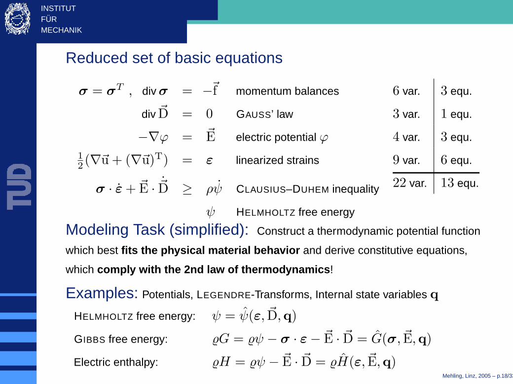
INSTITUTFURMECHANIK
Reduced set of basic equations
σ = σT , div σ = −~f momentum balances 6 var. 3 equ.
div ~D = 0 GAUSS’ law 3 var. 1 equ.
−∇ϕ = ~E electric potential ϕ 4 var. 3 equ.
12(∇~u + (∇~u)T) = ε linearized strains 9 var. 6 equ.
22 var. 13 equ.σ · ε + ~E · ~D ≥ ρψ CLAUSIUS–DUHEM inequality
ψ HELMHOLTZ free energy
Modeling Task (simplified): Construct a thermodynamic potential function
which best fits the physical material behavior and derive constitutive equations,
which comply with the 2nd law of thermodynamics !
Examples: Potentials, LEGENDRE-Transforms, Internal state variables q
HELMHOLTZ free energy: ψ = ψ(ε, ~D,q)
GIBBS free energy: G = ψ − σ · ε − ~E · ~D = G(σ, ~E,q)
Electric enthalpy: H = ψ − ~E · ~D = H(ε, ~E,q)Mehling, Linz, 2005 – p.18/33
INSTITUTFURMECHANIK
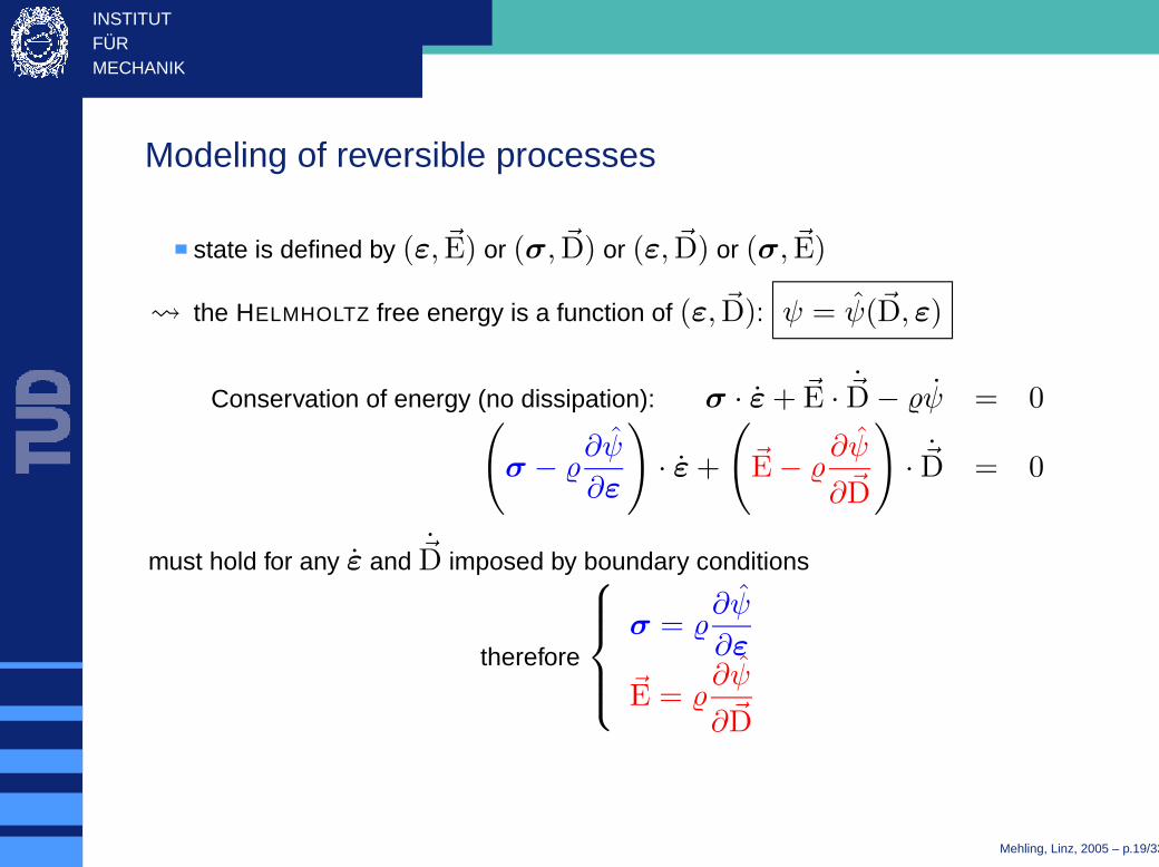
Modeling of reversible processes
state is defined by (ε, ~E) or (σ, ~D) or (ε, ~D) or (σ, ~E)
the HELMHOLTZ free energy is a function of (ε, ~D): ψ = ψ(~D, ε)
Conservation of energy (no dissipation): σ · ε + ~E · ~D − ψ = 0(
σ − ∂ψ
∂ε
)
· ε +
(
~E − ∂ψ
∂~D
)
· ~D = 0
must hold for any ε and ~D imposed by boundary conditions
therefore
σ = ∂ψ
∂ε
~E = ∂ψ
∂~D
Mehling, Linz, 2005 – p.19/33

INSTITUTFURMECHANIK Linear piezoelectric law
Quadratic form for ψpe:
ψpe(ε, ~D) =1
2ε · Cε − ε · lh~D +
1
2~D · β ~D
σ =∂ψpe
∂ε= Cε − lh~D
~E =∂ψpe
∂~D= −lhTε + β ~D
C Elastic stiffness at const. ~D
lh Tensor of piezoelectric coupling
β Dielectric compliance at const. ε
ε and ~D are given relative to the unloaded state.
Moduli C, β, lh are in general anisotropic
Moduli C, β considered isotropic in most models
lh is considerd transversely isotropic with respect to polarization direction
Quadratic electrostrictive lawCubic form for ψes:
ψes(ε, ~D) =1
2ε · Cε − ε · lh~D +
1
2~D · β ~D + ε · A(~D⊗ ~D)
Mehling, Linz, 2005 – p.20/33

INSTITUTFURMECHANIK Modeling irreversible processes (1)
Additional (internal) variables are necessary to describe the state of the material.
Decomposition of strains and electric displacements:
ε = εr + εi , ~D = ~Dr + ~Pi
εr, ~Dr: reversible, piezoelectric εi, ~Pi: irreversible, ferroelectric
The irreversible quantities are described by the set of internal state variables q
Free Energy:ψ = ψ(ε, ~D,q)
Clausius–Duhem inequality: σ · ε + ~E · ~D − ψ ≥ 0(
σ − ∂ψ
∂ε
)
· ε +
(
~E − ∂ψ
∂~D
)
· ~D −∑
j
∂ψ
∂qjqj ≥ 0
!!
!!
!!
!!
!!
!!
!!
!!
Remaining inequality: Driving forces for the internal variables
∑
j
−∂ψ
∂qjqj =
∑
j
fj qj ≥ 0 ⇒ qj = λfj , λ ≥ 0
fj : Driving forces
Mehling, Linz, 2005 – p.21/33
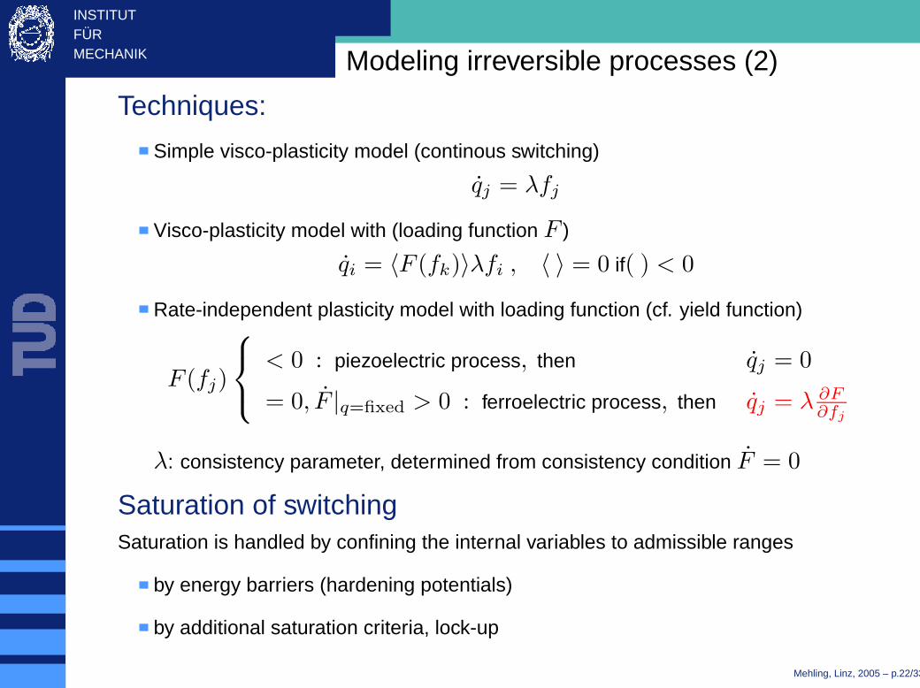
INSTITUTFURMECHANIK Modeling irreversible processes (2)
Techniques:
Simple visco-plasticity model (continous switching)
qj = λfj
Visco-plasticity model with (loading function F )
qi = 〈F (fk)〉λfi , 〈 〉 = 0 if( ) < 0
Rate-independent plasticity model with loading function (cf. yield function)
F (fj)
< 0 : piezoelectric process, then qj = 0
= 0, F |q=fixed > 0 : ferroelectric process, then qj = λ ∂F∂fj
λ: consistency parameter, determined from consistency condition F = 0
Saturation of switchingSaturation is handled by confining the internal variables to admissible ranges
by energy barriers (hardening potentials)
by additional saturation criteria, lock-up
Mehling, Linz, 2005 – p.22/33
INSTITUTFURMECHANIK
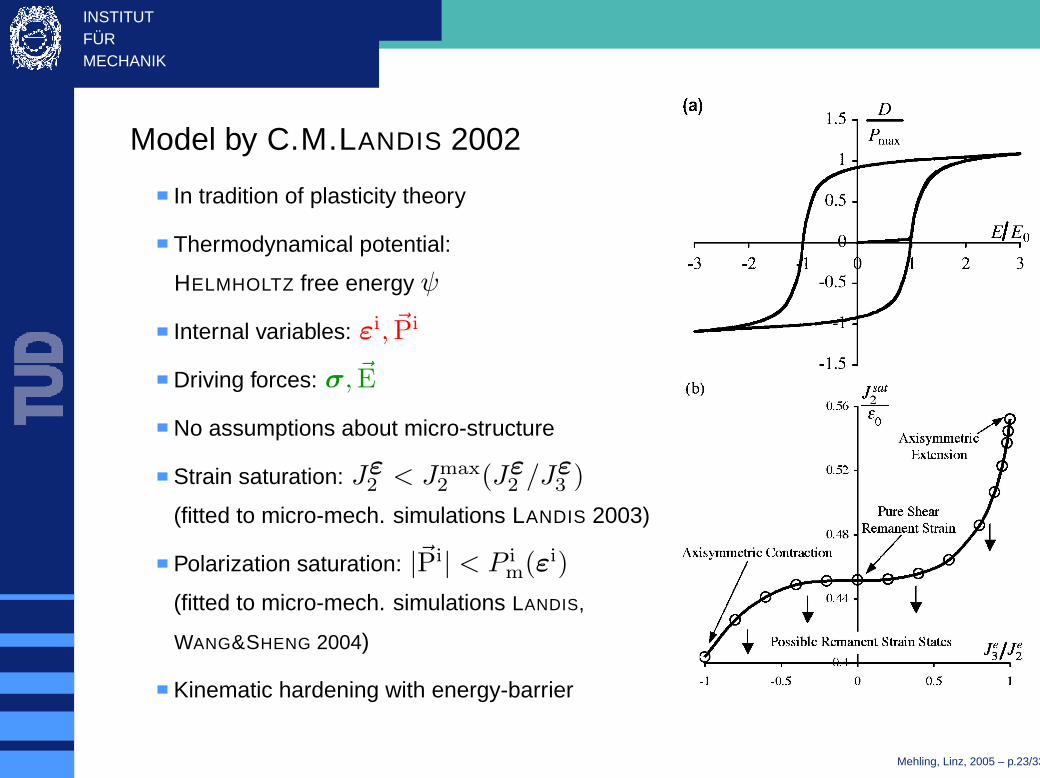
Model by C.M.LANDIS 2002
In tradition of plasticity theory
Thermodynamical potential:
HELMHOLTZ free energy ψ
Internal variables: εi, ~Pi
Driving forces: σ, ~E
No assumptions about micro-structure
Strain saturation: Jε2 < Jmax
2 (Jε2 /J
ε3 )
(fitted to micro-mech. simulations LANDIS 2003)
Polarization saturation: |~Pi| < P im(εi)
(fitted to micro-mech. simulations LANDIS,
WANG&SHENG 2004)
Kinematic hardening with energy-barrier
Mehling, Linz, 2005 – p.23/33

INSTITUTFURMECHANIK
Model by M.KAMLAH&JIANG 1999see presentation by Marc Kamlah!
Thermodyn. potential: GIBBS energy
Internal variables
β : Fraction of c-axis, within 45 -cone
γ : Measure for polarisation resulting from these c-axis
~eγ/β : later versions: Additional internal variables
for rotation of cone and polarization
Admissible states: 0 ≤ β ≤ 1 and |γ| ≤ β
Irreversible quantities:
εi(β) = ε03
2
β − β0
1 − β0
(
~n⊗~n −1
31
)
, ~Pi(γ) = P0γ~n
Later versions:
KAMLAH&JIANG 2002, KAMLAH&WANG 2003
~P
a
a
c
45
x
β = 1
γ = β
−γ = β
γ
β
∂G
1
-1
1
0
G
β0
Mehling, Linz, 2005 – p.24/33

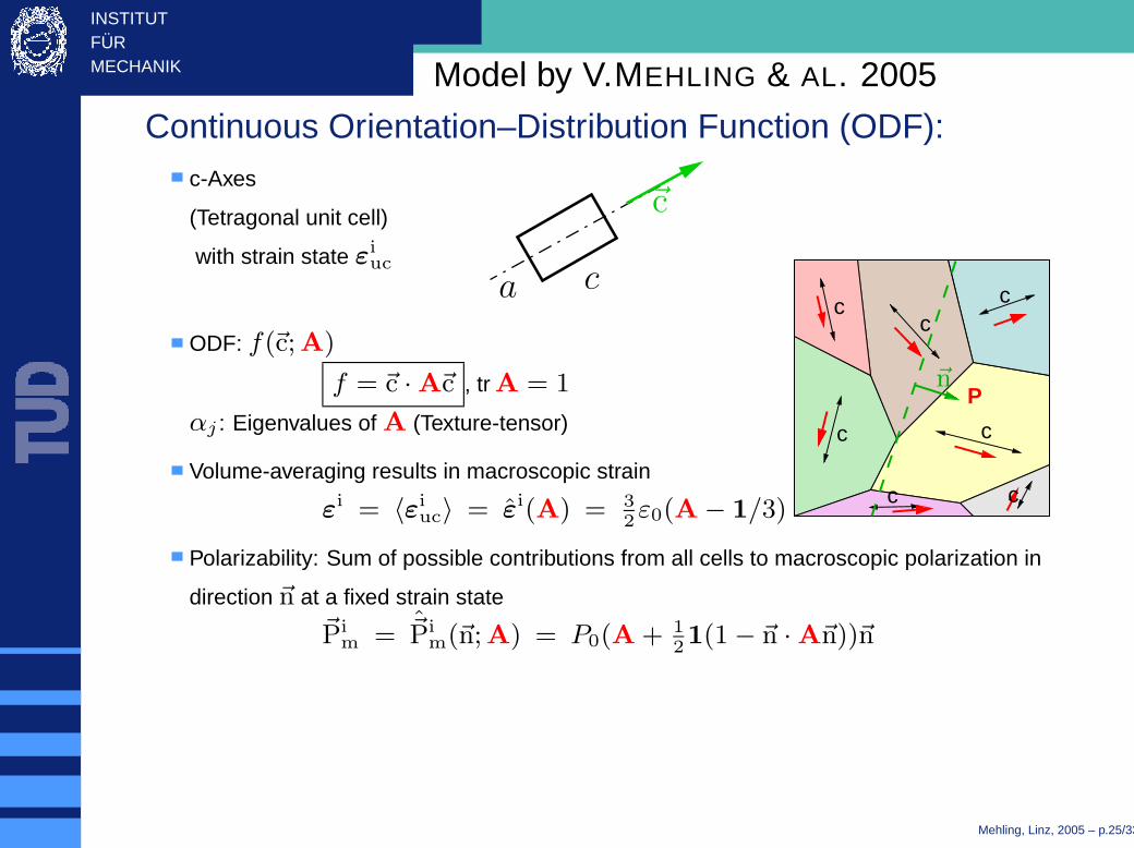
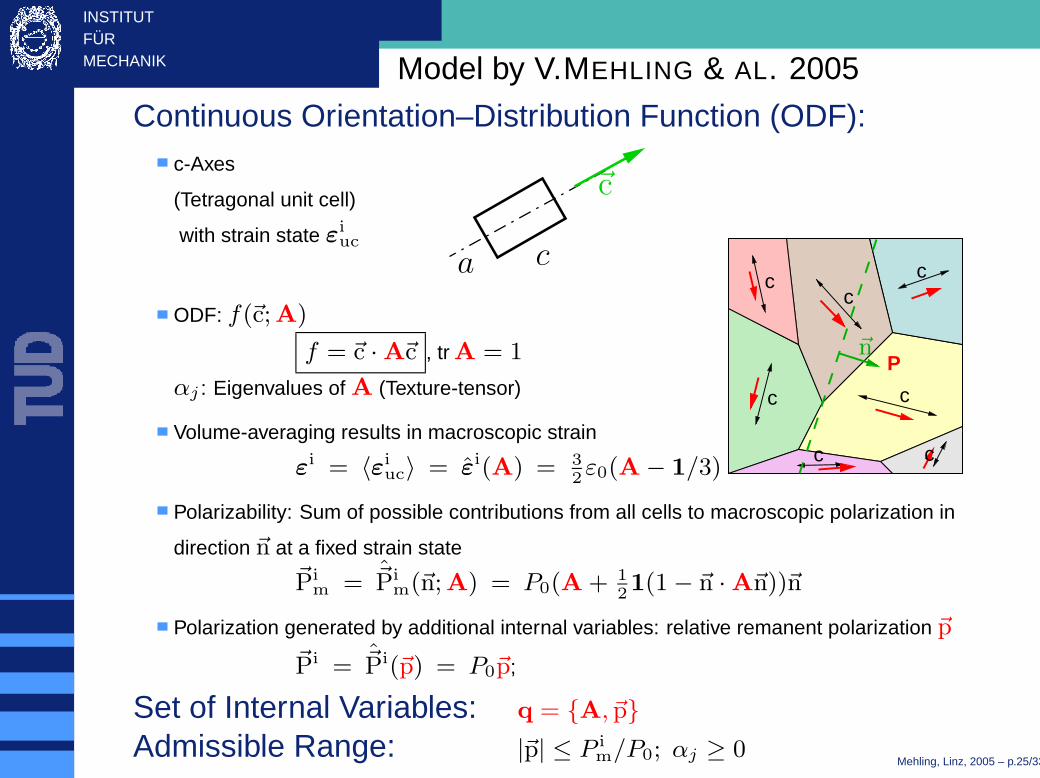
INSTITUTFURMECHANIK Model by V.MEHLING & AL. 2005
Continuous Orientation–Distribution Function (ODF):c-Axes
(Tetragonal unit cell)
c
a
~c-Achse
a
x2
x3
x1
~c~cwith strain state εi
uc
Mehling, Linz, 2005 – p.25/33

INSTITUTFURMECHANIK Model by V.MEHLING & AL. 2005
Continuous Orientation–Distribution Function (ODF):c-Axes
(Tetragonal unit cell)
ca
~c
Example: α1 = 0.95, α2 = 0.05, α3 = 0.0
~c
c1
c2
α2α1
f(~c,A)
ODF
with strain state εiuc
ODF: f(~c;A)
f = ~c · A~c , tr A = 1
αj : Eigenvalues of A (Texture-tensor)
Mehling, Linz, 2005 – p.25/33

INSTITUTFURMECHANIK Model by V.MEHLING & AL. 2005
Continuous Orientation–Distribution Function (ODF):c-Axes
(Tetragonal unit cell)
ca
~c
c
cc
c
c
c c
with strain state εiuc
ODF: f(~c;A)
f = ~c · A~c , tr A = 1
αj : Eigenvalues of A (Texture-tensor)
Volume-averaging results in macroscopic strain
εi = 〈εiuc〉 = εi(A) = 3
2ε0(A − 1/3)
Mehling, Linz, 2005 – p.25/33
INSTITUTFURMECHANIK Model by V.MEHLING & AL. 2005
Continuous Orientation–Distribution Function (ODF):c-Axes
(Tetragonal unit cell)
ca
~c
c
cc
c
c
c
P~n
c
with strain state εiuc
ODF: f(~c;A)
f = ~c · A~c , tr A = 1
αj : Eigenvalues of A (Texture-tensor)
Volume-averaging results in macroscopic strain
εi = 〈εiuc〉 = εi(A) = 3
2ε0(A − 1/3)
Polarizability: Sum of possible contributions from all cells to macroscopic polarization in
direction ~n at a fixed strain state
~Pim = ~Pi
m(~n;A) = P0(A + 121(1 − ~n · A~n))~n
Polarization generated by additional internal variables: relative remanent polarization ~p
~Pi = ~Pi(~p) = P0~p;
Set of Internal Variables: q = A, ~p
Admissible Range: |~p| ≤ P im/P0; αj ≥ 0
Mehling, Linz, 2005 – p.25/33

INSTITUTFURMECHANIK Model Summary (MEHLING, TSAKMAKIS, GROSS, 2005)
Internal variables, irrev. quantities q = A, ~p ,(
εi = εi(A), ~Pi = ~Pi(~p))
Additive decomposition ε = εr + εi; ~D = ~Dr + ~Pi
Electric enthalpy H = Hr(~E, ε, ~p) + H i(A, ~p)
Piezoelectric constitutive law Hr = Hr(Lk(~E, ε, ~p)) (cf. SCHRODER&GROSS 2004)
(invariant formulation) =1
2εr · CE(~p)εr − ε
r · e(~p)~E −1
2~E · ǫε(~p)~E
~D = −∂Hr/∂~E, σ = ∂Hr/∂ε
Hardening potential H i = H i(A, ~p)
Dissipation inequality, driving forces −∂H
∂A· A −
∂H
∂~p· ~p = f
A · A +~fp · ~p ≥ 0
(HUBER&FLECK 2001, LANDIS 1999)Coupled switching criterion F = (
‖dev (fA)‖
fAc
)2+(|~fp|
fpc
)2+φdev (fA)·(~p ⊗~fp)s
fAc fp
c
−1 ≤ 0
Evolution of internal variables A = λ∂F/∂fA, ~p = λ∂F/∂~fp , iff F = 0 and loading
Mehling, Linz, 2005 – p.27/33

INSTITUTFURMECHANIK
Numerical Implementationwww.DAEdalon.org
Implementation into standard-FEM
Nodal degrees of freedom: ux, uy, uz, ϕ (ALLIK&HUGHES, 1970)
Implicit time integration method
Predictor - corrector method
Linear/quadratic volume-elements
Material Constants (poled PZT4) for Piezo-Constants see DUNN&TAYA ’94
C11 = 139000MPa C12 = 77800MPa C44 = 25600MPa
C33 = 115000MPa C13 = 74300MPa
e333 = 15.1C/m2 e331 = −5.2C/m2 e131 = 12.7C/m2
ǫ11 = 646.4E-5C/MVm ǫ33 = 562.2E-5C/MVm
ε0 = 0.32% P0 = 0.36C/m2 Ec = 0.4MV/m σc = 35MPa
cA = 0.02MPa mA = 1 aA = 0.0001MPa
cp = 0.06MPa mp = 1 ap = 0.0006MPa φ = 2.0
Mehling, Linz, 2005 – p.28/33

INSTITUTFURMECHANIK
Example 1: Cyclic electric loadingwww.DAEdalon.org
E [MV/m]
D[C
/m²]
-2 -1 0 1 2-0.4
-0.2
0
0.2
0.4 0 MPaEσ
y
x
σ
E
E [MV/m]-2 -1 0 1 2
-0.002
-0.001
0
0.001
0.002
0.003
0.004
ε
0 MPa
(cf. experiment, e.g. LYNCH 1996)
Mehling, Linz, 2005 – p.29/33

INSTITUTFURMECHANIK
Example 1: Cyclic electric loadingwww.DAEdalon.org
...with constant mechanical compressive stress.
E [MV/m]
D[C
/m²]
-2 -1 0 1 2-0.4
-0.2
0
0.2
0.4 0 MPa-15 MPa Eσ
y
x
σ
E
E [MV/m]-2 -1 0 1 2
-0.002
-0.001
0
0.001
0.002
0.003
0.004
ε
0 MPa
-15 MPa
(cf. experiment, e.g. LYNCH 1996)
Mehling, Linz, 2005 – p.29/33

INSTITUTFURMECHANIK
Example 1: Cyclic electric loadingwww.DAEdalon.org
...with constant mechanical compressive stress.
E [MV/m]
D[C
/m²]
-2 -1 0 1 2-0.4
-0.2
0
0.2
0.4 0 MPa-15 MPa-30 MPa
Eσ
y
x
σ
E
E [MV/m]-2 -1 0 1 2
-0.002
-0.001
0
0.001
0.002
0.003
0.004
ε
0 MPa
-15 MPa
-30 MPa
(cf. experiment, e.g. LYNCH 1996)
Mehling, Linz, 2005 – p.29/33

INSTITUTFURMECHANIK
Example 1: Cyclic electric loadingwww.DAEdalon.org
...with constant mechanical compressive stress.
E [MV/m]
D[C
/m²]
-2 -1 0 1 2-0.4
-0.2
0
0.2
0.4 0 MPa-15 MPa-30 MPa-60 MPaσ
Eσ
y
x
σ
E
E [MV/m]-2 -1 0 1 2
-0.002
-0.001
0
0.001
0.002
0.003
0.004
ε
0 MPa
-15 MPa
-30 MPa
-60 MPa
(cf. experiment, e.g. LYNCH 1996)
Mehling, Linz, 2005 – p.29/33

INSTITUTFURMECHANIK
Example 2: Mechanical loadingwww.DAEdalon.org
mech. depolarization
σ
y
xP0
−σ
D [C/m 2]
σ[M
Pa]
-0.36-0.3-0.24-0.18-0.12-0.06
-70
-35
0
mech. cycling
ε
y
x
σ
ε
σ[M
Pa]
-0.0032 0 0.0032 0.0064-200
-100
0
100
200
300
mech. shear cycling
σ12
x
y
σ12
σ12
σ12
ε 12
-80 -40 0 40 80
-0.006
-0.003
0
0.003
0.006
[MPa]
Mehling, Linz, 2005 – p.30/33

INSTITUTFURMECHANIK
Example 3: Repolarization for ~E ∦ ~Pi
www.DAEdalon.org
Polarization response Strain response
E [MV/m]0 1 2 3
-0.001
0
0.001
0.002
0.003
0.004
ε
E [MV/m]D[C
/m2 ]
0 1 2 30
0.12
0.24
0.36
0.48
0.6
0.72
0°
45°
90°
135°
180°
α E
α
y
xP0
E
(cf. experiment, e.g. HUBER&FLECK 2001, ZHOU, 2003)
Mehling, Linz, 2005 – p.31/33

INSTITUTFURMECHANIK
Example 4: Polarization of a strip with holewww.DAEdalon.org
Vector of irreversible Polarization [C/m2] Vector of Electric Field Strength [MV/m]
0 2.5 5 7.5 10 12.5 15 17.5
−10
−5
0
x
Irrev. Polarisation Pi : Min.|P|= 0 Max.|P|= 0.34983
y
0 2.5 5 7.5 10 12.5 15 17.5
−10
−5
0
x
Elektric Field E : Min.|E|= 0.27167 Max.|E|= 5.1261
y∆ϕ
~D · ~n = 0
Mehling, Linz, 2005 – p.32/33

INSTITUTFURMECHANIK
Conclusion
Basic phenomenology and structure of ferroelectrics
Modeling through the length-scales
Overview over micromechanical modeling
Fundamentals of continuum thermodynamics & electrostatics
Thermodynamically consistent modeling
Piezoelectricity – Electrostriction – Ferroelectricity
Phenomenological models - three examples
Numerical examples
Mehling, Linz, 2005 – p.33/33