Embed Size (px)
Citation preview

1
Al-Mustansiriya University Dr Ali Al-Ghalib Civil Engineering Department
Course: Mechanics of Materials (Strength of Materia ls)
Two term course, number of hours: 4/week
Lecturer: Dr Ali Al-Ghalib
Academic year: 2014-2015, second year classes
Introduction
Mechanics of materials is the field of structural engineering, which studies the behavior of solid material under loads. In other words, the field of structural engineering that investigates the internal resistance and deformation of solid bodies subjected to loads.
P3 P1
S1
P1 P4
S2
P2
S3
P2 sectional plane P5
P1, P2, P3 … are external loads
If the whole body is under equilibrium condition, any part of whole body will also be under equilibrium. S1, S2, S3… are the internal forces that maintain the part of the body in equilibrium.
Mechanics of material subject deals with the forces S1, S2, S3… and their effects on the body.
Text Book
• Mechanics of Materials, second edition (SI version), by: E. Popov
• Introduction to Mechanics of Solids, by E. Popov
References
Solid body

2
Al-Mustansiriya University Dr Ali Al-Ghalib Civil Engineering Department
• Strength of Materials, fifth edition,(SI units), Schaum’s outlines, by: W. Nash and M. Potter
• Mechanics of Materials, sixth edition (U.S. customary and SI units), by: F. Beer, E. Johnston Jr, J. DeWolf and D. Mazurek
• Mechanics of Materials Volume 1 and 2, third edition, (SI units) by: E.J. Hearn
Syllabus (program)
Subject Chapter Page
Stress, Axial Loads 1 1
Strain, Hooke’s Law, Axial Load Problems 2 33
Axial Force, Shear and Bending moment 4 91
Torsion 3 57
Pure Bending of Beams 5 119
Shearing Stresses in Beams 6 163
Compound Stresses 7 199
Analysis of Plane Stress and Strain 8 235
Deflection of Beams 11 353
U.S. Customary Units and Their SI Equivalents
Quantity U.S. Customary SI Equivalent
Force lb. kip
4.448N 4.448kN
Length in ft
25.4mm 0.3048m
Area in2
ft2 645.2mm2
0.0929m2
Stress Ib/in2 (psi) 6.895kN/m2 (kPa)

3
Al-Mustansiriya University Dr Ali Al-Ghalib Civil Engineering Department
SI Prefixes
Multiplication factor Prefix Symbol
1012 Tera T
109 Giga G
106 Mega M
103 Kilo k
102 Hecto h
10-2 Centi c
10-3 Milli m
10-6 Micro µ
10-9 Nano n
10-12 Pico p

4
Al-Mustansiriya University Dr Ali Al-Ghalib Civil Engineering Department
Chapter One: Stress- Axial Loads
The concept of the stress
In the subject of mechanics of materials, we move from the explanation of forces to the term ‘stress’ because the effect of the force in the section suffers main disadvantage. In fact, any system of forces in a section can be represented as a force in a point. However, this force affects the whole section, or in other words this force influences all the points of the section not only the point where it is applied. Therefore, in the subject of mechanics of materials we determine the stress on the section instead of the force on the section.
Because of any force system on a section can be replaced by a general single force, this general force could be inclined force, hence can be resolved into normal (perpendicular) force and horizontal (parallel) force.
The intensity of the force normal to the surface of the section is called Normal stress σ.
While, the intensity of the force parallel to the surface of the section is called Shear stress τ.
P3 P1
S
P1 P4
F
P2
P2 sectional plane P5
� = lim∆�∆�∆
Where:
F is the force acting normal to the section (normal component of the force S)
A is the corresponding area of the element.
Solid body
V
ΔA

5
Al-Mustansiriya University Dr Ali Al-Ghalib Civil Engineering Department
= lim∆�∆�∆
Where:
V is the force acting parallel to the section (horizontal component of the force S)
A is the corresponding area of the element.
τthe intensity of the force parallel to the plane of section and called shear stress
Units of the stress (SI system)
N/m2 =Pa (Pascal), kN/m2 =kPa, MN/m2 =N/mm2 = MPa.
General stresses in a space element
In spatial infinitesimal element, there are 9 components of stress; 3 components are normal stresses and 6 components are shear stresses, as in the figure below:
σz
σx, σy,σz are normal stresses

6
Al-Mustansiriya University Dr Ali Al-Ghalib Civil Engineering Department
� ,��, �, �,��,� are shear stresses
In plane, there are 4 components of stresses; 2 normal stresses and 2 shear stresses, as in the plane element below:
But, this infinitesimal element is in equilibrium, therefore:
∑Mo = 0
Τxy (dy .dx) – Τyx (dx .dy) = 0
Τxy = Τyx
Consequently, shear stresses occur on perpendicular planes are equal; and as a result there are only 3 components of stresses on an infinitesimal element in plane; 2 normal stresses (σx, σy) and
one shear stress �
Types of stresses
1) Normal stresses
a) Tensile stress Where
P = axial (passes through the centroid) tensile force
A = cross-sectional area
When the applied force is axial and normal, a uniform (equal) maximum normal stress can be achieved through the section.
b) Compressive stress
7
Al-Mustansiriya University Dr Ali Al-Ghalib Civil Engineering Department
c) Bearing stress
The bearing stress is a normal compressive stress happens between two surfaces.
In this example, we have two bearing stresses. First, between the timber block and the steel base, this equals:
�� =� ���
120 ∗ 100
Second, between the steel base and the soil, this equals:
�� =� ��� ���
� ∗ �
2) Shear stress a) Direct shear stress
i. Single shear The best example for this type of stress can be given in the riveted joint applications. In the following example, the axial force is transferred from the plate A to plate B through the shear stress in the bolt.
���� =�
� !�
W1 W2
8
Al-Mustansiriya University Dr Ali Al-Ghalib Civil Engineering Department
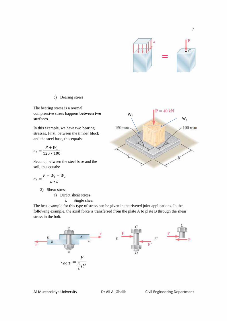
Failure of a bolt in single shear
ii. Double shear
���� ="#$
%&#
b) Punching shear stress
c) Torsional shear stress

9
Al-Mustansiriya University Dr Ali Al-Ghalib Civil Engineering Department
Example 1-1 page 12: Determine the bearing stress between the beam and wall. Also, calculate the normal stress in the bolts.
F.B.D for the beam:
'() = 0
10(3.5) = Rc (1) → Rc= 35kN
∑� = 0
RB + 10 =35 → RB = 25kN
• Normal stress on the bolt
����� =+,#�-./0 = ��.2∗�345$
%6�37#88# = 39.79(�< The stress in the threads zone of the bolt
����� =+,#�-./0 = ��.2∗�345$
%6�=7#88# = 62.17(�< The stress outside the threads zone of the bolt (critical
stress)
• Bearing stress at point C between the beam and the wall:
�? = @?�ABCDEF =35 ∗ 10HI
200JJ ∗ 200JJ = 0.875(�<

10
Al-Mustansiriya University Dr Ali Al-Ghalib Civil Engineering Department
Example 1-2:
Investigate the state of stress at level of 1.0m above the base.
Solution:
The normal stress at section a-a:
P = 20kN/m2 * 0.5m *0.5m = 5kN
W1 = [0.5+1.0]/2 m * 1.0m * 0.5m * 25kN/m3 = 9.4kN
Fa = P + W1 = 5 +9.4 = 14.4kN
σa = Fa/ Aa-a =14.4kN/ (1.0*0.5)m2 = 28.8kPa (compressive stress)
The bearing stress between the concrete block and the soil:
W = weight of the block = [0.5 + 1.5]/2 *2 *0.5 * 25 = 25kN
R = P + W = 5 + 25 = 30kN
σb = R/ Abase=30kN/ (1.5*0.5)m2 = 40kPa
Problem 1-14, page 29: find the maximum normal stress in the following rod.
0.5m0.5 0.5
2.0
m
W=20kN/m2
Side viewFront view
Concrete block
γc=25kN/m3
0.5
1.0
m
R

11
Al-Mustansiriya University Dr Ali Al-Ghalib Civil Engineering Department
∑Fx = 0
Ax = 310 +180 – 90 = 400kN
Stress @ sec 1-1:
��L� = 33M53.33�28# = 160000N�< = 160(�<
Stress @ sec 2-2:
��L� =90NI
0.0012J� = 75000N�< = 75(�<
Stress @ sec 3-3:
�HLH =180NI
0.0012J� = 150000N�< = 150(�<
Class work:
The two solid cylindrical steel rods AB and BC are welded together at B and loaded as shown in the figure. Knowing that the normal stress must not exceed 175MPa in rod AB and 150MPa in rod BC determine the smallest allowable values of d1 and d2.

12
Al-Mustansiriya University Dr Ali Al-Ghalib Civil Engineering Department
Riveted (Bolted) Joints
There are four types of stresses occur at riveted joints, these are:
1) Shearing stress in rivets 2) Tension stress in plate 3) Bearing stress between plate and rivet 4) Shearing stress in plate
• Shearing stress in rivets
Assumption:
Shearing stress in rivets is equal and uniform. This assumption is approximately true because the shearing stresses are actually distributed in a non-uniform way across the area of the cut.
Example:
Frivet = P/3
CDOA� = P/H�/ 6&7#
Example:
According to the assumption, the shear stress must be equal in the three rivets.
Therefore, the shear forces must be different.
CDOA� = �R/46!�� � !�� � !H�7
�� = CDOA� ∗ � !��
�� = CDOA� ∗R4 !�
�
�H = CDOA� ∗R4 !H
�
Example:
Double shear

13
Al-Mustansiriya University Dr Ali Al-Ghalib Civil Engineering Department
Frivet = P/4
CDOA� = �/4R/46!7�
• Tension stresses in plates
��7�L� = ��. T
��7�L� =�
6� U 2!V7. T
Where:
t = thickness of plate
dh = diameter of hole
dh = drivet + 3mm
��7�L� W ��7�L�
• Bearing stress between the plate and rivet
�� =�!. T =
�CDOA�!. T
PP
Plan
P
section
P
d
Frivet
Frivet
b

14
Al-Mustansiriya University Dr Ali Al-Ghalib Civil Engineering Department
Example:
For the lap joint shown in the figure,
Calculate the safe axial tensile force (P); if:
��7B���X = 136(�<
7B���X = 102(�<
��7B���X = 330(�<
Assume the diameter of hole =25mm.
Solution:
Shear force in rivet (Frivet) = P/4
= �CDOA�CDOA� =P �
!�= 102
Psafe = π (22)2 *102* 10-3= 155kN
��7B���X = �Y� − 46!V��A)ZT = 136
Psafe = [300-4(25)]* 6*136*10-3 = 163.2kN
��)B���X = �/4!. T = 330(�<
Psafe 4*22*6* 330*10-3 = 174.2kN
The safe force which does not cause failure neither in shear nor in tensile nor in bearing is Psafe = 155kN.
Allowable stresses; Factor of Safety
In design, the area of the member or element is the unknown, while the force is known. However, information on the parameter, stress, must be provided. In fact, information on the stress of material can be gathered from tests.
6[\N\]^\) = �6N\]^\)�6_[`aTb]\<�c`)

15
Al-Mustansiriya University Dr Ali Al-Ghalib Civil Engineering Department
Practically, the stress reaches its maximum value and the corresponding stress (at point D) is called ultimate stress. However, the stress value used in design is set significantly lower than the ultimate stress and known as allowable stress by use of factors of safety.
�<dT]e]fa<f`Tg = hcTbJ<T`aTe`aacc]^<�c`aTe`aa
Of course, the factor of safety must be greater than 1.0 if failure is to be avoided. Depending upon the circumstances, factors of safety from slightly above 1.0 to as much as 10 are used.

16
Al-Mustansiriya University Dr Ali Al-Ghalib Civil Engineering Department
Homework
1. The axial member shown in the figure is made of steel and has an allowable axial compressive stress of 100MN/m2.
a) What is the allowable axial compressive force P1 if P2 = 200kN? b) What is the allowable axial compressive force P1 if P2 = 80kN?
Answer: a) P1 = 60kN; b) P1 = 150kN.
2. For the lever mechanism shown in the figure below, find the necessary diameter for the bolt of pin B such that the allowable shearing stress in this bolt does not exceed 100MPa.
Answer: d=18mm (d=16.43mm)

17
Al-Mustansiriya University Dr Ali Al-Ghalib Civil Engineering Department
Chapter Two: Strain- Hooke’s Law- Axial Load Proble ms
The normal strain (ε) is the ratio of the total deformation (∆) to the total length (L) of the member.
i = ∆j
This type of strain is also known as axial strain or linear strain. As deformation and length are given in the same units, the normal strain (ε) obtained by dividing ∆ by L is a dimensionless quantity. Strains are very small values and could be read in micros (µ).
e.g.ε=0.00025 = 250x10-6 (or ε=250µ)
True Stress- strain diagram
Tensile testing machine
Stress-strain diagram for a typical structural steel in tension (not to scale)

18
Al-Mustansiriya University Dr Ali Al-Ghalib Civil Engineering Department
True stress � = P� (ordinate scale)
Strain i = ∆k (x-axis)
Ductile and Brittle Materials
Metallic engineering materials are commonly classified as either ductile or brittle materials. A ductile material lis one having a relatively large tensile strain up to the point of rupture (for example, structural steel or aluminum) whereas a brittle material has a relatively small strain up to this same point. An arbitrary strain of 0.05 mm/mm is taken as the dividing line between these two classes of materials. Cast iron and concrete are examples of brittle materials.
Stress-strain diagrams of two typical ductile materials
Stress-strain diagram of a typical brittle material

19
Al-Mustansiriya University Dr Ali Al-Ghalib Civil Engineering Department
Proportional Limit
The ordinate of the point A is known as the proportional limit, i.e., the maximum stress that may be developed during a simple tension test such that the stress is a linear function of strain. For a brittle material having the stress-strain curve shown in last Figure, there is no clear proportional limit.
Yield Point
The ordinate of the point B in the Figure, denoted by σy, at which there is an increase in strain with no increase in stress, is known as the yield point of the material.
Ultimate Strength or Tensile Strength
The ordinate of the point D in the Figure, the maximum ordinate to the curve, is known either as the ultimate strength or the tensile strength of the material.
Hooke’s Law
For any material having a stress-strain curve of the form shown in the first three Figures, The relation between stress and strain is linear for comparatively small values of the strain. This linear relation between elongation and the axial force causing it is called Hooke’s law. To describe this initial linear range of action of the material we may consequently write:
� = li Where: E denotes the slope of the straight-line portion OA of each of the curves in the three Figures.
The quantity E, i.e., the ratio of the unit stress to the unit strain, is the modulus of elasticity of the material in tension, or, as it is often called, Young’s modulus of elasticity.
Robert Hooke
Robert Hooke (1635–1703) was an English scientist who performed experiments with elastic bodies and developed improvements in timepieces (watches). He also formulated the laws of gravitation independently of Newton, of whom he was a contemporary. Upon the founding of the Royal Society of London in 1662, Hooke was appointed its first curator.

20
Al-Mustansiriya University Dr Ali Al-Ghalib Civil Engineering Department
Deflection of Axially Loaded Rods (applied within e lastic range only)
This general axially loaded rod has different axial loads and different cross-sectional areas. For the infinitesimal element of original length dx, the new length is dx+∆dx.
For the whole rod:
∆= m ∆!n)� .But, i = ∆&�
&� or ∆!n = i!n
∆= m i�)� !n = m op
q)� !n
∆= r ��!nl�)
�
This equation is used to calculate the deflection between points A and B, when the cross-sectional area (Ax) and/or axial load (Px) and/or modulus of elasticity (Ex) are changing constantly between points A and B.
Special cases:
1.
∆= �jl
2.
21
Al-Mustansiriya University Dr Ali Al-Ghalib Civil Engineering Department
∆���B�= P-k-q-�- � Psksqs�s � Pt/kt/
qt/�t/or∆���B�= ∑ Pukuqu�u
EDv�
Where: n= no. of segments where all parameters, the axial force, cross-sectional area and modulus of elasticity, are constant within the segment length itself.
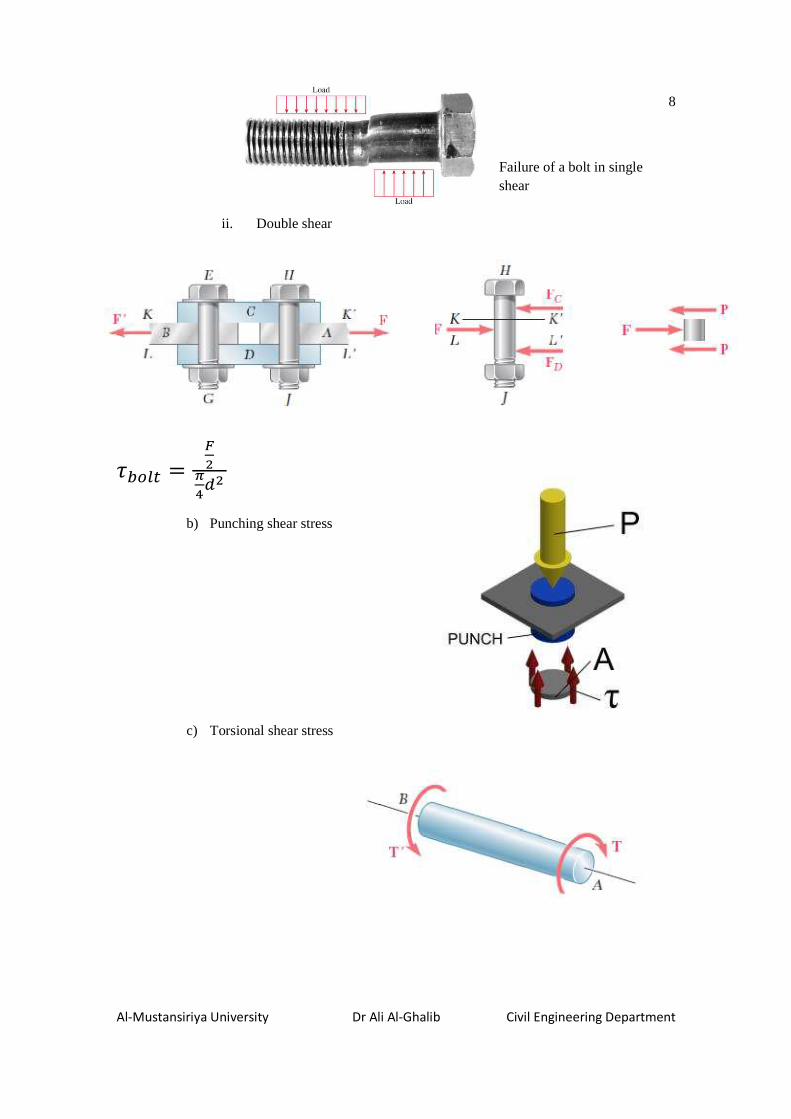
Example: For the rod of variable cross-sectional area and different materials shown below, find the maximum safe force (P) such that the total deflection is 0.5mm (shortening).
Based upon the allowable stresses:
For bronze: 3P = σb)allow * A b→ 3P = 120 N/mm2 * 500mm2 → P = 20kN
For steel: 2P = σs)allow * A s→ 2P = 140 N/mm2 * 320mm2 → P = 22.4kN
For aluminum: 2P = σal)allow * A al→ 2P = 75 N/mm2 * 640mm2 → P = 24kN
Based upon the total deflection:
∆���B�='�DjDlDDH
Dv�
−0.5 = − 3� ∗ 40085000 ∗ 500 −
2� ∗ 50070000 ∗ 640 +
2� ∗ 600210000 ∗ 320
-0.5 = -2.82*10-5P -2.23*10-5P +1.78*10-5P
-0.5 = -3.27*10-5P
P = 15.29kN
Therefore, Psafe = 15.29kN
Aluminum
100x100mm
Eal =70kN/mm2
steel
50x50mm
Es =200kN/mm2
P

22
Al-Mustansiriya University Dr Ali Al-Ghalib Civil Engineering Department
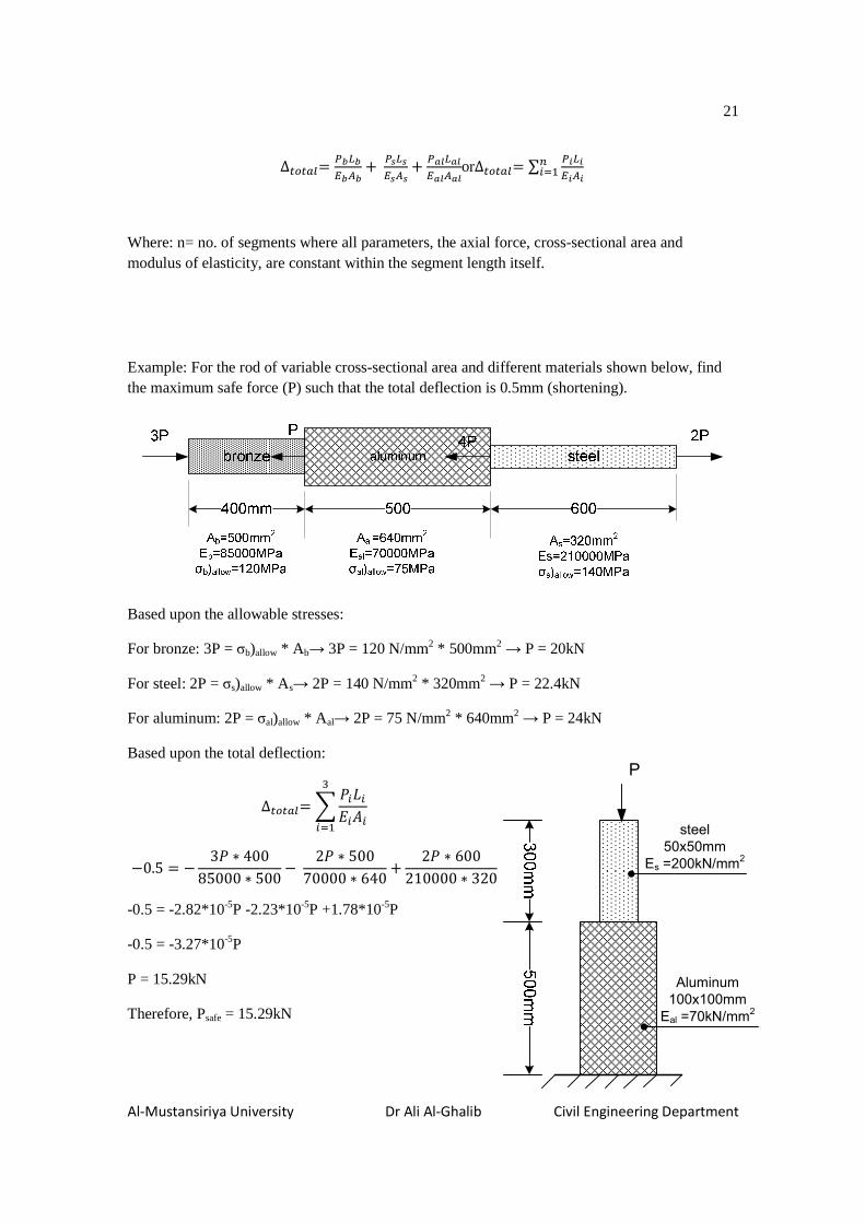
Example:
For the composite column shown:
1. Determine the maximum load P if the total deflection ∆=0.25mm. 2. Draw the vertical deflection diagram.
∆���B�= �jwlww ��jB�lB�B�
0.25 = �6300JJ7200NI/JJ�650n507JJ� � �6500JJ7
70NI/JJ�6100n1007JJ�
0.25= 0.0006P + 0.00071P
P = 190.8kN
∆B�= �jB�lB�B� =190.865007706100n1007 = 0.136JJ
∆w= �jwlww =190.863007200650n507 = 0.114JJ
Example: A rigid bar ABC, shown in Figure, is suspended by a pin at B, and loaded by a vertical force P. At A, a 10-mm-diameter steel tie rod AD connects the section to a firm ground support at D. Use E = 200GPa.Determine the vertical deflection at C.
Solution:
∑MB = 0
TAD (30) = 200 (40)
TAD = 266.67kN
40cm30cm
20cm
A B C
P=200kN
D

23
Al-Mustansiriya University Dr Ali Al-Ghalib Civil Engineering Department
∆�x= yz{∗kq∗� = �==.=|∗�33
�33∗�/ 6�37# = 3.4JJ
From the symmetry of triangles:
∆} 3 =
∆z{H3
∆C=40*∆AD/30;
∆C= 4.53mm.
Example: Determine the horizontal and vertical displacements of joint B. Assume that the normal stress in the members AB and BC are equal.
Solution: For joint B:
∑Fy = 0; �√��)? = � ⇒ �)? = √2�6d]J�e`aab]\)
∑Fx = 0; ��) = √2� � �√�� = �6T`\ab]\)
Given: σAB = σBC
��) =
√2�)?
)? = √2�)
∆�)= �z,kz,qz,�z, =
Pkq� 6lc]\�<Tb]\)
∆)?= �)?j)?l)?)? =
√2� ∗ √2jl ∗ √2
= √2�jl ∗ 6�]\Te<dTb]\)
Displacement of joint B:
∆))� = ∆�)= �jl
A BC=?,
E
∆ BC
∆B )V
P
40cm30cm
TAD

24
Al-Mustansiriya University Dr Ali Al-Ghalib Civil Engineering Department
∆)7� = g� � g� = 1√2∆)? �
1√2∆)? � ∆�)
∆)7� = 1√2 ∗
√2�jl � 1
√2 ∗√2�jl � �j
l
∆)7� = 3�jl
Statically indeterminate members (axially loaded on ly)
Example: The suspended composite rod shown in the figure is subjected to an axial force P=400kN. Determine the total deflection occurs in this rod considering that the two materials, steel and aluminum, act as one unit.
Solution:
Equilibrium equation, ∑Fy=0
Pal+Ps = 400 …… (1)
We have two unknowns and one equilibrium equation only!
We need to set another equation
∆al = ∆s……(Compatibility equation)
�B�jB�lB�B� =�wjwlww
�B� ∗ 75070 ∗ 300 = �w ∗ 750210 ∗ 300
3�B� = �� …… (2) Compatibility equation
Solve both equations (1) and (2) simultaneously:
Pal =100kN; Ps =300kN
Therefore, ∆total = ∆al = ∆s

25
Al-Mustansiriya University Dr Ali Al-Ghalib Civil Engineering Department
∆B�= �B�jB�lB�B� =100NI ∗ 750JJ
70NI/JJ� ∗ 300JJ� = 3.571JJ
∆w= �wjwlww =300NI ∗ 750JJ
210NI/JJ� ∗ 300JJ� = 3.571JJ
∆total = ∆al = ∆s =3.571mm
Check the stresses:
�B� = �B�B� =100 ∗ 10HI300JJ� = 333.3(�<
�w = �ww =300 ∗ 10HI300JJ� = 1000(�<
Example: A square reinforced concrete column of (300x300)mm cross-section with 8 reinforcing steel bars is subjected to a compressive force of 800kN. Find the compressive stress in both materials, steel and concrete, if Es=210kN/mm2, Ec=14kN/mm2. Compare these stresses with the allowable stresses, which are:
σc)allow= 0.25f’c (f’c=30MPa), σs)allow= 140MPa.
Solution:
Equilibrium equation, ∑Fy=0
Pc + Ps = 800
�� ∗ � � �w ∗ w = 800⋯⋯617 We have two unknowns, Pc and Ps, and one equilibrium equation only!
We need to set another equation
εc = εs……(Compatibility equation)
��l� =�wlw
�w = lwl� ∗ �� ⇒ �w = \�� Where: \ = J]![c<ee<Tb]\ = qsq� n = 15; �w = 15��⋯⋯627 �� ∗ � � 15�� ∗ w = 800

26
Al-Mustansiriya University Dr Ali Al-Ghalib Civil Engineering Department
As = 8[π/4(16)2] = 1608mm2
Ac = (300)2 – 1608 = 88392mm2
800*103 = σc(88392) + 15σc(1608)
σc = 7.11MPa < 7.5MPa (0.25*30MPa) O.K.
σs = 15* 7.11= 106.65MPa < 140MPa O.K.
Example: Determine the reactions at A and B for the steel bar and loading shown in the Figure, assuming a close fit at both supports before the loads are applied.
Solution:
Equilibrium equation: ∑Fy = 0;
RA + RB =900kN …. (1)
Compatibility equation, the total deformation of the bar is zero.
∆total = 0.
0 = �z∗�23q∗�23 � 6�zLH337∗�23q∗�23 � 6�zLH337∗�23
q∗ 33 − �,∗�23q∗ 33
0.6@� � 0.6@� − 180 � 0.375@� − 112.5 − 0.375@) = 0
1.575@� − 0.375@) = 292.5⋯(2) Compatibility equation
Substitute equation (1) into equation (2) gives:
1.575@� − 0.3756900 − @�7 = 292.5
1.95RA = 630; RA = 323kN.
RB = 900-323 = 577kN.
A
D
C
B
300kN
600kN
A=250mm2
A=400mm2

27
Al-Mustansiriya University Dr Ali Al-Ghalib Civil Engineering Department
Problems Involving Temperature Changes (Thermal cha nges)
Axial deflection due to the temperature change is:
∆= � ∗ j ∗ ∆�
Where:
α= coefficient of thermal expansion 1/◦C
L = original length
∆T= change in temperature (Tfinal-Tinitial) ◦C
Rising in temperature causes ∆=+ (extension), while dropping in temperature causes ∆=- (contraction).
i�VAC8B� = ∆j = � ∗ ∆�
��VAC8B� = � ∗ ∆� ∗ l
The effect of temperature changing is only important in statically indeterminate members. This means, temperature change causes stresses and strains only in indeterminate elements, while determinate elements elongate and shrink freely without any stress and strain.
Example: Find the thermal stress exists in fixed steel bar when the temperature rises 50◦C. Use α=12*10-6/◦C
Solution:
i�VAC8B� = � ∗ ∆�
��VAC8B� = � ∗ ∆� ∗ l
σthermal = 12*10-6/◦C* 50◦C* 200*103N/mm2= 120MPa.
To clarify how the internal thermal stresses develop, remove the right-hand support to allow the steel bar elongates freely, as in the figure.
∆�V= � ∗ j ∗ ∆�=12*10-6*50 *1000
∆=0.6mm.
∆�V= �jl⇒ 0.6 = � ∗ 1000
200 ∗ 100
1000mm
28
Al-Mustansiriya University Dr Ali Al-Ghalib Civil Engineering Department
P=12kN; ��V = P� = ��3335
�3388# = 120(�<
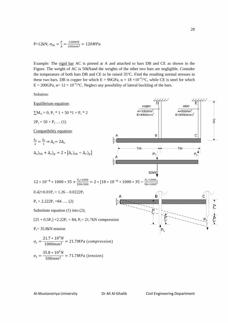
Example: The rigid bar AC is pinned at A and attached to bars DB and CE as shown in the Figure. The weight of AC is 50kNand the weights of the other two bars are negligible. Consider the temperature of both bars DB and CE to be raised 35°C. Find the resulting normal stresses in these two bars. DB is copper for which E = 90GPa, α = 18 ×10–6/°C, while CE is steel for which E = 200GPa, α= 12 × 10–6/°C. Neglect any possibility of lateral buckling of the bars.
Solution:
Equilibrium equation:
∑MA = 0; Pc * 1 + 50 *1 = Ps * 2
2Ps = 50 + Pc…. (1)
Compatibility equation:
∆s� = ∆�
� ⇒∆w= 2∆� ∆w7�V � ∆w7� = 2 ∗ �∆�7�V − ∆�7��
12 ∗ 10L= ∗ 1000 ∗ 35 � Ps∗�333�33∗233 = 2 ∗ Y18 ∗ 10L= ∗ 1000 ∗ 35 − P�∗�333
�3∗�333] 0.42+0.01Ps = 1.26 – 0.0222Pc
Ps + 2.222Pc =84 …. (2)
Substitute equation (1) into (2);
[25 + 0.5Pc] +2.22Pc = 84; Pc= 21.7kN compression
Ps= 35.8kN tension
�� = 21.7 ∗ 10HI1000JJ� = 21.7(�<6d]J�e`aab]\7
�w = 35.8 ∗ 10HI500JJ� = 71.7(�<6T`\ab]\7

29
Al-Mustansiriya University Dr Ali Al-Ghalib Civil Engineering Department
Poisson’s Ratio
When a bar is subjected to a simple tensile loading there is an increase in length of the bar in the direction of the load, but a decrease in the lateral dimensions perpendicular to the load. The ratio of the strain in the lateral direction to that in the axial direction is defined as Poisson’s ratio. It is denoted by the Greek letter ν (Nu).
ν = �c<T`e<caTe<b\<nb<caTe<b\ � = −i i� = − i�i�
This property is constant for the material within elastic range, just such as the modulus of elasticity (E).For most metals it lies in the range 0.25 to 0.35. For cork, n is very nearly zero.
ν= 0.1-0.16 concrete
ν= 0.25steel
ν= 0.333aluminum
ν= 0.5rubber
Generalized Hooke’s Law
Consider an element of an isotropic material in the shape of a cube subjected to a triaxial tensile stress, as shown in the figure. By using the principal of superposition, the general Hooke’s law can be written as:
i� = ��l − �� l − � ��l
i = � l − � ��l − ���l
i� = ��l − ���l − �� l
Final shape
Initial shape

30
Al-Mustansiriya University Dr Ali Al-Ghalib Civil Engineering Department
Example: A piece of a steel plate of (250 x 50 x 10)mm dimensions is subjected to a biaxial force system in x and y directions, as shown in the figure. Knowing that E=200000MPa and ν =0.25:
a) What is the change in the thickness b) To cause the same change in thickness as in (a) by Px alone, what must be its magnitude?
Solution:
Pp�p =a) �� =
�33∗�34523∗�388# = 200(�<
� = � =
200 ∗ 10HI250 ∗ 10JJ� = 80(�<
�� = 0
i� = ��l − � ��l − � � l = −�l ��� � � � = −0.25
200 ∗ 10H 6200 � 807 i� = −0.00035
∆� = i� ∗ TℎbdN\`aa = −0.00035 ∗ 10JJ = −0.00356d]\Te<dTb]\7
b) ∆� = −0.0035JJ ε� = −0.00035
σ� = σ = 0;σ� =? 6[\N\]^\7 i� = ��l − � ��l − � � l
−0.00035 = −0.25 ∗ ��200 ∗ 10H⇒ �� = 280(�<
�� = �� ∗ � = 280 IJJ� ∗ 650 ∗ 107JJ�
Px = 140kN.

31
Al-Mustansiriya University Dr Ali Al-Ghalib Civil Engineering Department
Example: Knowing that Poisson’s ratio ν=0.25, Determine the magnitude of a single system of force acting only in the y-direction that would cause the same deformation in the y-direction as the initial forces.
Solution:
�� = 180 ∗ 10HI100 ∗ 75JJ� = 24(�<
� = 200 ∗ 10HI50 ∗ 100JJ� = 40(�<
�� = −240 ∗ 10HI50 ∗ 75JJ� = −64(�<
i = � l − � ��l − ���l
i = 1l �40 − 0.25624) − 0.256−64)�
i = +50l
�� = �� = 0;� =?[\N\]^\
i = +� l
50l = �
l ⇒ � = 50(�<
Py = 50*103N/mm2*(50*100)mm2 = 250kN
Example:
What material should be used in order to produce a cube has no change in its volume when it is subjected to a uniform pressure?
Solution: σx =σy=σz =σ
i� = 0 = − oq + � o
q + � oq
0 = − oq 61 − 2�); oq ≠ 0
1 − 2� = 0⇒ � = 12
σ
σ
σ

32
Al-Mustansiriya University Dr Ali Al-Ghalib Civil Engineering Department
Shear Strain
Shear stresses acting on an element of material (Figure -a) are accompanied by shear strains. The shear stresses have no tendency to elongate or shorten the element in the x, y, and z directions. In other words, the lengths of the sides of the element do not change. Instead, the shear stresses produce a change in the shape of the element (Figure- b). The original element, which is a rectangular parallelepiped, is deformed into an oblique parallelepiped, and the front and rear faces become rhomboids.
Because of this deformation, the angles between the side faces change. For instance, the angles at the points q and s, which were π/2 before deformation, are reduced by a small angle γ to π/2-g (Figure- b). At the same time, the angles at points p and rare increased to π /2+ γ. The angle γ is a measure of the distortion, or change in shape, of the element and is called the shear strain. Because shear strain is an angle, it is usually measured in degrees or radians.
Hooke’s Law in Shear
For many materials, the initial part of the shear stress-strain diagram is a straight line through the origin, just as it is in tension. For this linearly elastic region, the shear stress and shear strain are proportional, and therefore we have the following equation for Hooke’s law in shear:
= ��
In which, G is the shear modulus (also called the modulus of rigidity).The moduli of elasticity in tension and shear are related by the following equation:
� = l261 � �7

33
Al-Mustansiriya University Dr Ali Al-Ghalib Civil Engineering Department
QUIZ № 1 (2nd December 2013)
Determine the axial stresses developed in the steel and aluminum rods when the temperature of the system drops 40◦C. Take αs=11.7x10⁻⁶/◦C and αAl=23x10-6/◦C.
Solution:
Compatibility equation:
|∆s| = |∆Al |
∆s)p - ∆s)T = ∆Al)T – ∆Al)p
�wjwlww − �w∆�jw =���∆�j�� − ���j��l���� �w61000721061007 − 11.7 ∗ 10L= ∗ 40 ∗ 1000
= 23 ∗ 10L= ∗ 40 ∗ 1000 − ���61000)706300)
�w21 − 0.468 = 0.92 − ���
21
Ps + PAl = 29.15 ….. (1)
Equilibrium equation:
Ps = PAl ….. (2) Substitute equation (1) into (2):
2Ps = 29.15 => Ps = PAl = 14.57kN
σs = 145.7MPa
σAl = 48.57MPa

34
Al-Mustansiriya University Dr Ali Al-Ghalib Civil Engineering Department
QUIZ № 1(2nd December 2013)
The horizontal rigid beam AD is supported by hinge at D and vertical bars BE and CF, as shown in the figure below. The bars BE and CF are made of steel (E=200GPa) and have cross-sectional areas ABE=11100mm2 and ACF=9280mm2. Determine the vertical displacement of point A.
Solution:
Equilibrium equation:
∑MD=0
FBE(3.5) +FCF(1.5)=600 (5.5)
FCF+ 2.33FBE = 2200…. .(1)
Compatibility equation:
∆)q3.5 = ∆?�1.5
∆)q= 2.33∆?�=> �)q ∗ 3000200 ∗ 11100 =�?� ∗ 2400200 ∗ 9280
FBE = 2.235FCF…. (2)
Substitute equation (2) into (1):
FCF+ 2.33[2.235FCF] =2200; FCF =354.5kN and FBE =792.1kN.
∆)q=792.1 ∗ 3000200 ∗ 11100 = 1.07JJ
∆�5.5 =
∆)q3.5 => ∆�= 5.5
3.5 ∗ 1.07 = 1.68JJ
Solution of Q2 of midyear examination, year 2014: A compressive load P is transmitted through a rigid plate to three magnesium-alloy bars that are identical except that initially the middle bar is slightly shorter than the other bars, as shown in Figure 2. All the dimensions and properties of the assembly are shown in Figure 2.
P=600kN
A DCB
2.0m 2.0m 1.5m
E
F
1mm
Rigid plate
P
A=
3000
mm
2
E=
45G
Pa
A=3
000m
m2
E=
45G
Pa
A=3
000m
m2
E=
45G
Pa L=
1m

35
Al-Mustansiriya University Dr Ali Al-Ghalib Civil Engineering Department
a) Calculate the load P1 required to close the gap. b) Calculate the downward displacement of the rigid plate when P= 400kN.
Figure 2
Solution: Due to the symmetry of the system, the rigid plate moves vertically in a straight horizontal way.
a) In order to find the axial force (F) that causes 1mm shortening in the bar:
∆= �jl => 1JJ = � ∗ 1000JJ
2M588# ∗ 3000JJ�
F=135kN
Equilibrium equation: ΣFy=0; P1=2F=2*135=270kN
b) Now, the rigid plate is supported by three symmetrical bars, as shown in the figure:
Pr = 400-270 = 130kN
Equilibrium equation: ΣMo=0; F left_bar=F right_bar=F1
Equilibrium equation: ΣFy=0; Pr =2F1+F2=130kN…….1
Compatibility equation: ∆�= ∆�
��kq� = ��k
q� => �1 = �2……….2
Substitute equation 1 into 2:
F1=130/3= 43.33kN
∆= ��∗kq∗� = H.HHM5∗�33388
%��� #∗H33388# = 0.321JJ
Therefore, the total displacement of the rigid plate =1mm+0.321mm= 1.321mm
Rigid plate
P1
F F
L=1m
1mm
Rigid plate
Pr=400-P1A
=30
00m
m2
E=
45G
Pa
A=
3000
mm
2
E=
45G
Pa
A=
3000
mm
2
E=
45G
Pa L=
1m
F1 F1F2
o x

36
Al-Mustansiriya University Dr Ali Al-Ghalib Civil Engineering Department
Solution of Q1 of midyear examination, year 2015: A rigid beam AB of 2m length is hinged at A and supported by two wires attached at B (Figure 1). Both wires have same diameter (d=25mm), and are made of steel (Es=200GPa).
c) Determine the tensile stress in the wires due to the load P=100kN acting at point B. d) Find the downward displacement at the end of the rigid beam ∆B.
'(� = 0;
�� ∗ 1√2 ∗ 2 � �� ∗ 1
√2 ∗ 2 − 100 ∗ 2 = 0
From the symmetry of steel wires; one can write down a compatibility equation (∆wire1= ∆wire2). Hence, T1=T2=T.
T=70.7kN
a)
�XDCA = � = 70.7 ∗ 10HI
� 6257�JJ� = 144(�<
b)
∆XDCA= �jl = 70.7 ∗ 10HI ∗ 1414JJ
200 ∗ 10H(�< ∗ � 625)�JJ� = 1.02JJ
∆)= ∆XDCAd]a45 =
1.02JJ�√�
= 1.414JJ
37
Al-Mustansiriya University Dr Ali Al-Ghalib Civil Engineering Department
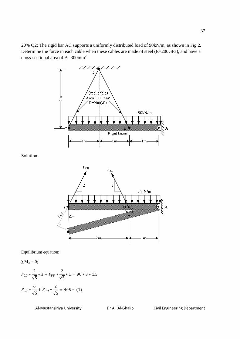
20% Q2: The rigid bar AC supports a uniformly distributed load of 90kN/m, as shown in Fig.2. Determine the force in each cable when these cables are made of steel (E=200GPa), and have a cross-sectional area of A=300mm2.
Solution:
∆C
D
∆B
D
Equilibrium equation:
∑MA = 0;
�?x ∗ 2√5 ∗ 3 � �)x ∗ 2
√5 ∗ 1 = 90 ∗ 3 ∗ 1.5
�?x ∗ 6√5 � �)x ∗ 2
√5 = 405⋯ 61)

38
Al-Mustansiriya University Dr Ali Al-Ghalib Civil Engineering Department
Compatibility equation:
∆�3 = ∆)1 => ∆?= 3∆)
∆?x ∗ √52 = 3 ∗ ∆)x ∗ √52
∆?x= 3 ∗ ∆)x
�?x ∗ √5l = 3 ∗ �)x ∗ √5l
�?x = 3 ∗ �)x⋯627 Substitute Eq.2 into Eq.1:
3 ∗ �)x ∗ =√2 � �)x ∗ �
√2 = 405
FBD=45.3kN
FCD=3 *FBD=3*45.3=135.8kN
20% Q2: The three steel bars shown in the figure support the horizontal rigid member. If a vertical load of 15kN is applied in the position shown, determine the axial force developed in each bar. Bars AB and EF each has a cross-sectional area of 50mm2, and bar CD has a cross-sectional area of 30mm2. Neglect the weight of the rigid beam. Use E=210GPa.

39
Al-Mustansiriya University Dr Ali Al-Ghalib Civil Engineering Department
Solution:
Equilibrium equation: ΣFy=0; FAB + FCD + FEF = 15 … … 1
Equilibrium equation: ΣME=0; [F AB (0.8)+ FCD (0.4) = 15(0.6)]/0.4
2FAB + FCD = 22.5…….2
Compatibility equation:
∆�) − ∆q�0.8 = ∆?x − ∆q�0.4
∆�) − ∆?x= 26∆?x − ∆q�) ∆�)= 2∆?x − ∆q�
��)j�)l�)�) = 2 �?xj?xl?x?x −
�q�jq�lq�q�
¡��)50 = 2�?x30 − �q�
50 ¢ ∗ 50
FAB= 3.33FCD - FEF … … 3
Solve Equation 1 and Equation 3 simultaneously:
FAB + FCD + FEF = 15 … … 1
FAB - 3.33FCD + FEF = 0 … … 3
4.33FCD =15
FCD = 3.46kN
From Equation 2:
2FAB + FCD = 22.5…….2
FAB = 9.52kN
From Equation 1
FAB + FCD + FEF = 15 … … 1
9.52 + 3.46 + FEF = 15
FEF = 2.02kN

40
Al-Mustansiriya University Dr Ali Al-Ghalib Civil Engineering Department
Homework
1. A tubular post of outer diameter d2 is guyed by two cables fitted with turnbuckles (see figure). The cables are tightened by rotating the turnbuckles, thus producing tension in the cables and compression in the post. Both cables are tightened to a tensile force of 110kN. The allowable compressive stress in the post is σc=35MPa. If the wall thickness of the post is 15mm, what is the minimum permissible value of the outer diameter d2? Answer: (d2)min=131mm.
2. A circle of diameter 225mm is engraved on the unstressed aluminum plate of thickness t=18mm. Forces acting in the plane of the plate later cause normal stresses σx=80MPa and σy=140MPa. For E=70GPa and ν=0.333, determine the change in (a) the length of diameter AB, (b) the length of diameter CD, (c) the thickness of the plate.
3. Two cylindrical rods, one of steel and the other of brass, are joined at C and restrained by rigid supports at A and E. For the loading shown and knowing that Es =200GPa and Eb =105GPa, determine (a) the reactions at A and E, (b) the deflection of point C.
4. A specimen of a methacrylate plastic is tested in tension at room temperature (see figure), producing the stress-strain data listed in the accompanying table. Plot the stress-strain curve and determine the proportional limit, modulus of elasticity and yield stress at 0.2% offset. Is the material ductile or brittle? Answer: σpl≈47MPa, slope≈2.4GPa; σy≈53MPa; Brittle.
375m
m

41
Al-Mustansiriya University Dr Ali Al-Ghalib Civil Engineering Department
Stress-Strain Data for Problem 4
Stress (MPa) Strain 0.0 0.0 8.0 0.0032 17.5 0.0073 25.6 0.0111 31.1 0.0129
39.8 0.0163 44.0 0.0184 48.2 0.0209 53.9 0.0260 58.1 0.0331 62.0 0.0429 62.1 Fracture
5. The data shown in the accompanying table were obtained from a tensile test of high-strength steel. The test specimen had a diameter of 12.87mm and a gage length of 51mm. At fracture, the elongation between the gage marks was 3.058mm and the minimum diameter was 10.7mm. Plot the conventional stress-strain curve for the steel and determine the proportional limit, modulus of elasticity, yield stress at 0.1% offset, ultimate stress, percent elongation in 51mm, and percent reduction in area. Answer: σpl≈448MPa; slope≈207GPa; σy≈475MPa; σu≈780MPa; Elongation=6%; Reduction=31%.

42
Al-Mustansiriya University Dr Ali Al-Ghalib Civil Engineering Department
Load N Elongation mm 0 0.0 4450 0.0051 8900 0.0153 26700 0.0484 44500 0.0841 53400 0.1 57400 0.1096 59622 0.1198 60512 0.1376 61402 0.1605 62291 0.2293 64071 0.2599 67631 0.3312 74750 0.586 81869 0.8561 88988 1.292 99666 2.823 100556 Fracture
6. For the axial steel rod shown below, determine the required force (P) to just close a gap of 0.5mm. (Take E=200kN/mm2), Answer: P=66.667kN.
7. The three bars shown in the figure support the vertical load of 20kN. The bars are joined
by the pin at A. Calculate the stress in each bar. The outer bars are each of brass and of cross-sectional area 2.5cm2. The central bar is steel and of area 2cm2. For brass, E=85GPa and for steel, E=200GPa. Answer: σb=16.8MPa, σs=79MPa.
2m

43
Al-Mustansiriya University Dr Ali Al-Ghalib Civil Engineering Department
8. The rigid bar AD is pinned at A and attached to the bars BC and ED, as shown below. The entire system is initially stress-free and the weights of all bars are negligible. The temperature of bar BC is lowered 25°C and that of bar ED is raised 25°C. Find the normal stresses in bars BC and ED. For BC, which is brass, assume E = 90GPa, α = 20 × 10–6 /°C, and for ED, which is steel, take E= 200GPa and α = 12 × 10–6/°C. The cross-sectional area of BC is 500mm2 and of ED is 250mm2.Answer: σs=43.9MPa, σb=52.6MPa.
9. The three-bar truss ABC shown in the figure has a span L=3m and is constructed of steel pipes having cross-sectional area A=3900 mm2and modulus of elasticity E=200GPa. Identical loads P act both vertically and horizontally at joint C, as shown below. (a) If P = 650kN, what is the horizontal displacement of joint B? (b) What is the maximum permissible load value Pmax if the displacement of joint B is limited to 1.5mm? Answer: (a) ∆B=2.5mm; (b) Pmax=390kN.

44
Al-Mustansiriya University Dr Ali Al-Ghalib Civil Engineering Department
10. A rigid bar of weight W= 800N hangs from three equally spaced vertical wires (length L=150mm, spacing a=50mm): two of steel and one of aluminum. The wires also support a load P acting on the bar. The diameter of the steel wires is ds= 2 mm, and the diameter of the aluminum wire is da=4 mm. Assume Es=210GPa and Eal=70GPa.
a) What load Pallow can be supported at the midpoint of the bar (x= a) if the allowable stress in the steel wires is 220MPa and in the aluminum wire is 80MPa? (see figure part a.)
b) What is Pallow if the load is positioned at x= a/2? (see figure part a.) c) Repeat (b) above if the second and third wires are switched as shown in figure part b.
Answer: a) Pallow=1504N; b) Pallow=820N; c) Pallow=703N.

45
Al-Mustansiriya University Dr Ali Al-Ghalib Civil Engineering Department
Chapter Three: Torsion
Torsion refers to the twisting of a straight bar when it is loaded by torques or twisting moments(T) that tend to produce rotation about the longitudinal axis of the bar. For example, when you turn a screwdriver (Figure), your hand applies a torque T to the handle and twists the rod of the screwdriver.
The SI unit for moment is the Newton meter (N .m).
An idealized case of torsional loading is pictured in Figure-a, which shows a straight bar supported at one end and loaded by two pairs of equal and opposite forces.
The moment of a couple may be represented by a vector in the form of a double-headed arrow (Figure-b).The direction (or sense) of the moment is indicated by the right-hand rule, using your right hand, let your fingers rotate in the direction of the moment, and then your thumb will point in the direction of the vector.
An alternative representation of a moment is curved arrow acting in the direction of rotation (Figure-c).

46
Al-Mustansiriya University Dr Ali Al-Ghalib Civil Engineering Department
Torsion formula of circular sections
Assumptions:
1. A plane section before twist remains plane after twist. 2. The distribution of shear strain (γ) through the section is linear.
3. The material of the body is linear elastic.
Length of the arc qq’ = rφ;
Also, length of arc qq’ = Lγ.
�8B� = e£j
And, 8B� = ¤C¥k [Linear variation of shear stress distribution along the radius]
r

47
Al-Mustansiriya University Dr Ali Al-Ghalib Civil Engineering Department
Torque T= stress*area*arm
dA =2π ρ dρ use θ=φ/L
� = r 62R¦7¦!¦BCAB
� = r 62R¦76�¦§7¦!¦BCAB
� = 2R�§ r¦H!¦C
� = 2R�§ e 4
� = R2 �§e
Polar moment of inertia
¨ = r ¦�!¦BCAB
¨ = r62R¦)¦�!¦C
3
¨ = 2Rr¦H!¦C
3=> ¨ = 2R e
4
¨ = Re 2
T=J G θ
As θ=φ/L
© = �j�¨
8B� =�e yk¤ªj => 8B� = �e
¨
ρ
dρτ
T
o

48
Al-Mustansiriya University Dr Ali Al-Ghalib Civil Engineering Department
Hollow circular sections
¨ = R2 6e� − e� 7
8B� = �e�¨
Cases for using of torsion formula:
1. © = yk¤ª Compare with ∆= Pk
q�
2. © = ∑ yuku¤uªu
EDv� Compare with ∆= ∑ Pukuqu�u
EDv�
Example 1:
Determine the maximum shearing stress occurs in the circular shaft AC.
8B� = �e¨
¨ = Re 2
2
1

49
Al-Mustansiriya University Dr Ali Al-Ghalib Civil Engineering Department
J=π/2(5)4=981.7mm4
8B� = 30 ∗ 10HIJJ5JJ981.7JJ = 152.8(�<
Example 2:
A circular hollow shaft with an outside diameter of 20mm and inside diameter of 16mm is subjected to a torque of 40Nm. Determine the torsional shear stress at the outside surface and inside surface of the shaft.
¨ = �� 6e� − e� 7
¨ = R2 610 − 8 7 = 9274JJ
8B� = �«� = �e�¨ = 40 ∗ 10HIJJ ∗ 10JJ
9274JJ = 43.13(�<
8DE = DE = �e�¨ = 40 ∗ 10HIJJ ∗ 8JJ
9274JJ = 34.51(�<
Example 3:
The steel shaft shown below is subjected to two concentrated torques at B and C. If the shear modulus of the steel material G is 80GPa, determine:
1. The angle of twist at the free end (total angle of twist). 2. The maximum shear strain in the shaft.
Solution:
1. ¨�) = �� �@�«� −@DE � = �
� 620 − 15 ) = 171806JJ
50
Al-Mustansiriya University Dr Ali Al-Ghalib Civil Engineering Department
¨)? = R2 6@ 7 =
R2 615 7 = 79521.5JJ
Φ� = Φ�) � Φ)�
= yk¤ª |�) � yk
¤ª |)? = − ��3∗�34∗2333∗�34∗�|�3=� ��3∗�34∗|33
3∗�34∗|�2��.2
= -0.00764+0.0132= 0.00556rad.
2. 8B� = yCª
8B�7�) = 210 ∗ 10HIJJ ∗ 20JJ171806JJ = 24.45(�<
Check the shear stress at BC:
8B�))? = 120 ∗ 10HIJJ ∗ 15JJ79521.5JJ = 22.64(�<
�8B� = � . 23333 = 0.0003e<!
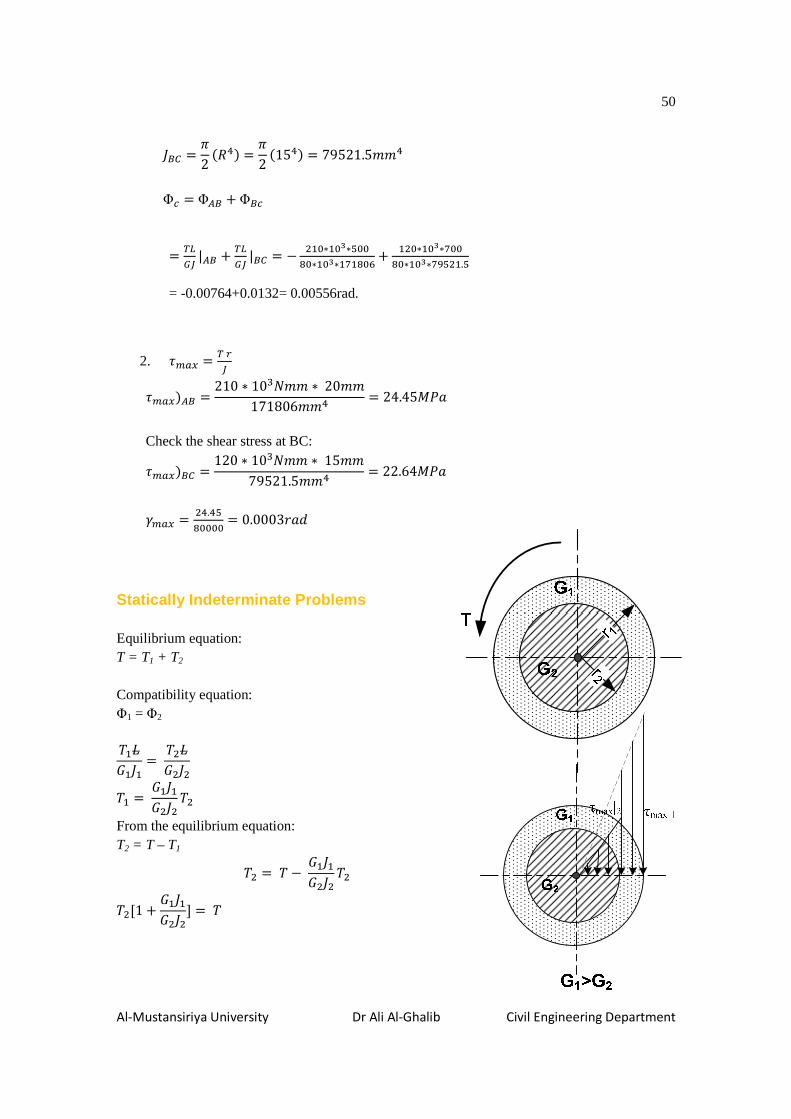
Statically Indeterminate Problems Equilibrium equation: T = T1 + T2
Compatibility equation: Φ1 = Φ2 ��j�� �
= ��j��¨� �� = �� �
��¨� ��
From the equilibrium equation: T2 = T – T1
�� = � −�� ���¨� ��
��[1 + �� ��� �
Z = �
51
Al-Mustansiriya University Dr Ali Al-Ghalib Civil Engineering Department
�� ∗ ¡�� � � �� ���¨� ¢ = �
�� = ¡��¨�∑�¨¢ ∗ �
�� = ®¤¯ª¯∑¤ª° ∗ �
Φ = ��j��¨� =®¤#ª#∑¤ª° �j��¨�
Φ = �j∑�¨
8B�|� = ��e��
8B�|� = ��e�¨�
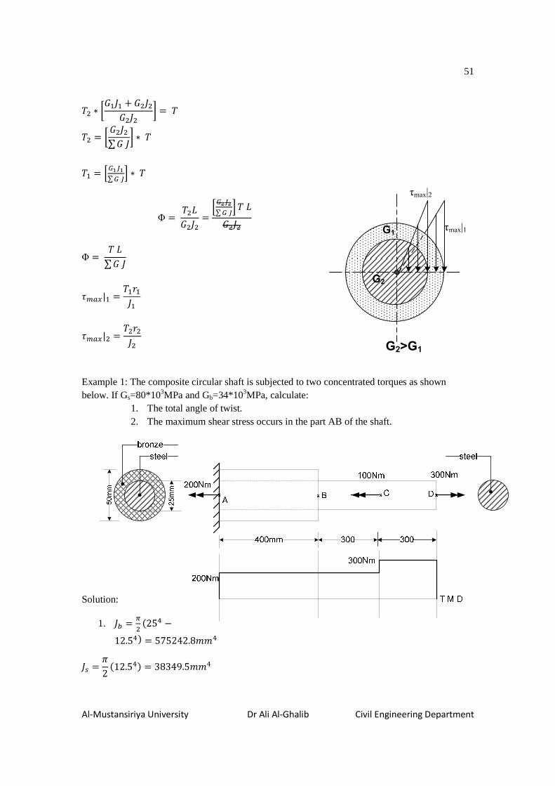
Example 1: The composite circular shaft is subjected to two concentrated torques as shown below. If Gs=80*103MPa and Gb=34*103MPa, calculate:
1. The total angle of twist. 2. The maximum shear stress occurs in the part AB of the shaft.
Solution:
1. ¨� = �� 625 −12.5 7 = 575242.8JJ
w = R2 612.5 ) = 38349.5JJ
G1
G2
τmax|2
τmax|1
G2>G1

52
Al-Mustansiriya University Dr Ali Al-Ghalib Civil Engineering Department
'�¨ = �w w � ��¨� = 80 ∗ 10H ∗ 38349.5 + 34 ∗ 10H ∗ 575242.8
'�¨ = 2.263 ∗ 10�3IJJ�
Φx = Φ�) + Φ)� +Φ?x
= �j∑�¨ |�) +
�j�¨ |)? +
�j�¨ |?x
= 200 ∗ 10H ∗ 4002.263 ∗ 10�3 + 200 ∗ 10H ∗ 300
80 ∗ 10H ∗ 38349.5 +300 ∗ 10H ∗ 300
80 ∗ 10H ∗ 38349.5 = 0.0524e<!
2. �w = ¤sªs∑¤ª ∗ � = 3∗�34∗HH �.2�.�=H∗�3¯± ∗ 200 = 27.11IJ
�� = ��¨�∑�¨ ∗ � = 34 ∗ 10
H ∗ 575242.82.263 ∗ 10�3 ∗ 200 = 172.85IJ
8B�|w = �weww= 27.11 ∗ 10H ∗ 12.5
38349.5 = 8.8(�<
8B�|� = ��e�¨� = 172.85 ∗ 10H ∗ 25
575242.8 = 7.5(�<
Example 2: A prismatic circular shaft AB is made of steel having shearing modulus G and radius r. Ends A and B are rigidly fixed. Determine the maximum shear stress in both regions, AC and BC, due to the torsional moment T applied at C. Solution: Since there are two unknowns TA
and TB, another equation (based upon deformations) is required. This is set up by realizing that the angular rotation at C is the same if we determine it at the right end of CB or the left end of AC. Compatibility equation: Φ�? = Φ)� �j�¨ |�? =
�j�¨ |)?

53
Al-Mustansiriya University Dr Ali Al-Ghalib Civil Engineering Department
��<�¨ = �)��¨
�� =�< �)
From the equilibrium equation: T = TA + TB
� = �< �) ��)
� = Y� � << ]�)
�) = Y<j]�
�� = Y�j]�
8B�|�? = ��e¨
8B�|)? = �)e¨
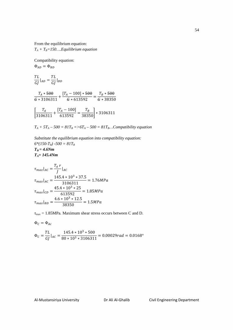
Example 3: A stepped solid circular steel shaft has the shape shown in the figure below and is having G=80*103MPa. The region AC is having D=75mm region CD having D=50mm, and region BD having D=25mm. Determine the maximum shearing stress occurs in the shaft as well as the angle of twist at C where a torsional load of 100N m is applied. Ends A and B are rigidly clamped.
¨�? = R2 637.5 7 = 3106311JJ
¨?x = R2 625 7 = 613592JJ
¨)x = R2 612.5 7 = 613592JJ
500mm 500mm500mm
x xxx100Nm 50NmTA TB
A DC B
D=75mm
D=25mmD=50mm
TMD
TA
TA -100
TA -150 TB
54
Al-Mustansiriya University Dr Ali Al-Ghalib Civil Engineering Department
From the equilibrium equation: TA + TB=150….Equilibrium equation Compatibility equation: Φ�x = Φ)x �j�¨ |�x = �j
�¨ |)x
�� ∗ 500� ∗ 3106311 �
Y�� − 100] ∗ 500� ∗ 613592 = �) ∗ 500� ∗ 38350
² ��3106311 �Y�� − 100]613592 = �)38350³ ∗ 3106311
TA + 5TA – 500 = 81TB =>6TA – 500 = 81TB…Compatibility equation Substitute the equilibrium equation into compatibility equation: 6*(150-TB) -500 = 81TB TB = 4.6Nm TA= 145.4Nm
8B�|�? = ��e¨ |�?
8B�|�? = 145.4 ∗ 10H ∗ 37.53106311 = 1.76(�<
8B�|?x = 45.4 ∗ 10H ∗ 25613592 = 1.85(�<
8B�|)x = 4.6 ∗ 10H ∗ 12.538350 = 1.5(�<
τmax = 1.85MPa. Maximum shear stress occurs between C and D.
Φ? = Φ��
Φ? = �j�¨ |�? =
145.4 ∗ 10H ∗ 50080 ∗ 10H ∗ 3106311 = 0.00029e<! = 0.0168°

55
Al-Mustansiriya University Dr Ali Al-Ghalib Civil Engineering Department
Torsion of Noncircular Members
The formulas obtained in the last sections for the distributions of stress and estimation of angle of twist under a torsional moment apply only to members with a circular cross section. Such that, it is wrong to assume that the shearing stress in the cross section of a square bar varies linearly with the distance from the axis of the bar and is, therefore, largest at the corners of the cross section. As you will see presently, the shearing stress is actually zero at these points.
Since the face of the element perpendicular to the y- axis is part of the free surface of the bar, all stresses on this face must be zero. Referring to the figure shown
below: τyx=0; τyz=0. For the same reason, all stresses on the face of the element
perpendicular to the z axis must be zero, and we write τzx=0; τzy=0
The determination of the stresses in noncircular members subjected to a torsional loading is beyond the interest of this course. However, the results obtained from the mathematical theory of elasticity for straight bars with a uniform rectangular cross section is given in this section for convenience. Denoting by L the length of the bar, by a and b, respectively, the wider and narrower side of its cross section, (Figure), The maximum shearing stress occurs along the center line of the wider face of the bar and is equal to:
8B� = ��<��
Furthermore, the angle of twist is given as:
© = �j´<�H�

56
Al-Mustansiriya University Dr Ali Al-Ghalib Civil Engineering Department
a
The coefficients α and β depend only upon the ratio a/b and are given in the Table shown below for a number of values of that ratio.
a/b α β 1.0 0.208 0.141 1.2 0.219 0.166 1.5 0.231 0.196 2 0.249 0.229
2.5 0.258 0.249 3 0.267 0.263 4 0.282 0.281 5 0.291 0.291
10 0.312 0.312 ∞ 0.333 0.333
For very thin sections (i.e. a/b>>10), α = β = 1/3. Therefore, the maximum shearing stress of the rectangular bar is written as:
8B� = 3�<��
Additionally, the angle of twist is written as:
© = 3�j<�H�

57
Al-Mustansiriya University Dr Ali Al-Ghalib Civil Engineering Department
Thin-walled members with open cross sections
R
Slotted circular pipe
a = 2πR
b = t
Slotted square tube
a = 4(a-t)
b = t
Angle
a = 2a-t
b = t

58
Al-Mustansiriya University Dr Ali Al-Ghalib Civil Engineering Department
Example: Compare the angle of twist and maximum shear stress for three members of length (L) having a square section, a rectangular section and a circular section of same area. All members are subjected to same torque (T). The circular section is of 100mm diameter, and the rectangular section is 25mm wide.
Solution:
Square Rectangular Circular
A=7854mm2 A=7854mm2 A=π/4(d)2= π/4(100)2=7854mm2
a=b= 88.6mm a=314mm b=25mm
J= π/2(r)4= π/2(50)4= 9817500mm4
µ = ¶·¸¹º»¼ © = 3�j
<�H� © = �j�¨ © = �j
0.141688.6) � © = 3�j314625)H� © = �j
�9817500�
© = �j8696532� © = �j
1633781� © = �j9817500�
8B� = ��<�� 8B� = 3�
<�� 8B� = �e¨
½¾¹¿ = ¶À. ÁÀÂ6ÂÂ. Ã)» 8B� = 3�
314625)� 8B� = �650)9817500
½¾¹¿ = ¶ÄÅÅÆû 8B� = �
65351 8B� = �196350
Summary:
©CA��BEF�A > ©wÇ«BCA > ©�DC��A
8B�CA��BEF�A > 8B�wǫBCA > 8B��DC��A

59
Al-Mustansiriya University Dr Ali Al-Ghalib Civil Engineering Department
Example: For the thin-walled square shaft with a longitudinal slot shown in the figure below, determine the angle of twist at section 1-1 and section 2-2. Take G=84kN/mm2
80N m50N m
200mm 200mm 300mm 300mm
50mm
4mm1
1
2
2
slot
30N m
50N m
30N m
T.M.D+
-
Solution: The angle of twist for the rectangular section is: © = �j´<�H �
a= 4(50-4) = 184mm
b=4mm
∴ <� = 1844 = 46 > 10; ∴ ´ = 13
© = ' 3 ∗ �j<�H �
©�L� = 3 ∗ 50 ∗ 10HIJJ ∗ 200JJ184JJ ∗ (4JJ)H ∗ 84 ∗ 10HI/JJ� − 3 ∗ 30 ∗ 10HIJJ ∗ 600JJ184JJ ∗ (4JJ)H ∗ 84 ∗ 10HI/JJ�= −0.0243e<!
©�L� = − 3 ∗ 30 ∗ 10HIJJ ∗ 300JJ184JJ ∗ (4JJ)H ∗ 84 ∗ 10HI/JJ� = −0.0273e<!

60
Al-Mustansiriya University Dr Ali Al-Ghalib Civil Engineering Department
Homework
1. The composite circular shaft is subjected to a concentrated torque (T) at point B, as shown below. The region AB is made of bronze, while the region BC is made of steel and bronze. Knowing that the allowable shearing stress of steel τallow=80MPa and the allowable shearing stress of bronze τallow=60MPa, determine the maximum torque (T) that can be applied safely at B. Use Gs=80GPa and Gb=34GPa
2. The solid square steel shaft shown in the figure below is subjected to the torque at C. Determine the maximum shearing stress occurs in the shaft. Ends A and B are rigidly clamped.

61
Al-Mustansiriya University Dr Ali Al-Ghalib Civil Engineering Department
Chapter Four: Axial Force, Shear and Bending Moment Beam: the member that resists forces applied laterally or transversely to its axis, such as main members supporting floors of buildings.
In this chapter, we are going to determine the system of internal forces that maintains equilibrium for any beam system. Types of supports
1. Roller or link: this support resists forces lie on one line of action of known direction.
In this type of supports there is only one unknown reaction in the static equilibrium equations. For the inclined support, the ratio between the two components is fixed.
2. Pin or hinge: this support resists forces act in any direction of the plane. The ratio between the components is not constant (not as in the roller).
Beam Beam
Body
Link
Beams

62
Al-Mustansiriya University Dr Ali Al-Ghalib Civil Engineering Department
3. Fixed (clamped, built in) support
This support resists movement of any type in the plane. Translation and rotation are prohibited.
Types of loadings
1. Concentrated load: this load could be either a force or moment
2. Uniformly distributed load: this is given as an intensity force per unit length (N/m, kN/m…)
w1
w2
3. Uniformly (linearly) varying load: this load is most commonly produced by the lateral soil or water pressure.
Beam
Beam

63
Al-Mustansiriya University Dr Ali Al-Ghalib Civil Engineering Department
Classification of beams according to their supporti ng system
1. Simple beam or simply supported beam
2. Clamped beam or fixed-ended beam

64
Al-Mustansiriya University Dr Ali Al-Ghalib Civil Engineering Department
3. Restrained beam (one fixed and one simple ends)
4. Cantilever beam
5. Overhanging beam
6. Continuous beam
For all beams the distance (L) between supports is called span
Classification of beams according to their analysis procedure
I. Unstable beams

65
Al-Mustansiriya University Dr Ali Al-Ghalib Civil Engineering Department
Number of unknown reactions = 2
Number of Equilibrium equations= 3, which are:
∑Fx = 0
∑Fy = 0
∑Mo = 0
When No. of unknowns < No. of Equilibrium equations, the beam is known as unstable beam
II. Stable and statically determinate beams
Number of unknown reactions = 3
Number of Equilibrium equations= 3, which are:
When No. of unknowns = No. of Equilibrium equations, the beam is known as stable and statically determinate beam
III. Stable and statically indeterminate beams
Number of unknown reactions = 5 and 4, respectively
Number of Equilibrium equations= 3, which are:
When No. of unknowns > No. of Equilibrium equations, the beam is known as stable and statically indeterminate beam

66
Al-Mustansiriya University Dr Ali Al-Ghalib Civil Engineering Department
Calculations of beams’ reactions
Example 1:
∑Fx = 0
Ax = 6kN
∑MA = 0
RB (8) = 8(4) + 6(7) +14
RB = 11.0kN
∑Fy = 0 +
Ay + 11 -8 -6 = 0
Ay = 3kN
Example 2:
The internal hinge always adds additional Equilibrium equation to the three original Equilibrium equations that is:
∑Mhinge = 0
Part BC
∑Mc = 0
4(1) – RB(2) = 0 => RB = 2kN
∑Fy = 0 +
Cy + 2 - 4 = 0
Cy = 2kN
Part AC
∑Fy = 0 +
Ay - 6 - 2 = 0
Ay = 8kN

67
Al-Mustansiriya University Dr Ali Al-Ghalib Civil Engineering Department
∑MA = 0
MA = 6(2) +2(2) = 16kN.m
∑Fx = 0
Ax = 0
Example 3:
Answer:
RA= 5600N
RB = 11200N
Internal forces and moments in beams
The part to the left of section 1-1
∑Fy = 0 +
5 - V = 0
V = 5kN
M = 5 (1) = 5kN.m
The part to the right of section 1-1:
V = 10-5 = 5kN
A B
10kN
2.0m 2.0m
1
1
5kN 5kN
1m
A B
8000
N/m
4.2m

68
Al-Mustansiriya University Dr Ali Al-Ghalib Civil Engineering Department
M = 5(3) – 10(1) = 5kN.m
Whether the left part of the section or the right part is taken, we must arrive at the same internal force results.
There are three types of internal forces in the plane as follows:
• Axial force (P), which algebraically equals the summation of all the axial forces exist on one side of the section.
• Shear force (V), which equals the algebraic summation of all the forces that exist perpendicularly on one side of the section.
• Bending moment (M), which equals the algebraic summation of the moments caused by all the perpendicular forces affect one side of the section.
Sign convention
Axial force (P)
Tensile (+)
Compressive (-)
Shear force (V)
At the right-hand side of the segment, downward (+)
At the right-hand side of the segment, upward (-)
Bending moment (M)
If the moment causes concave, that moment should be considered (+)
If the moment causes convex, that moment should be considered (-)

69
Al-Mustansiriya University Dr Ali Al-Ghalib Civil Engineering Department
Shear and moment diagrams by equations
Example 1: Draw the axial, shear force and bending moment diagrams by using equations for the beam shown below.
1) 0 ≤ x ≤ 5m
∑Fx = 0 =>P = 3kN compression
∑Fy = 0 =>V = +2kN constant
∑Mo = 0 =>M- 2(x) = 0 =>M = +2x linear
2) 5m ≤ x ≤ 10m
∑Fx = 0=>P = 0
∑Fy = 0 =>2 – 4 – V = 0 =>V = -2 constant
∑Mo = 0 =>M- 2(x) + 4(x-5) = 0 =>M = 20-2x linear

70
Al-Mustansiriya University Dr Ali Al-Ghalib Civil Engineering Department
General notes
• The three diagrams (axial, shear and bending moment) must end at zero because this is the condition that satisfies equilibrium.
• The points of concentrated force and/or concentrated moment and the points of supports are deliberate points that breaking the continuity of a period.
Example 2: Draw the shear force and bending moment diagrams by using equations for the simple beam shown below.

71
Al-Mustansiriya University Dr Ali Al-Ghalib Civil Engineering Department
0 ≤ x ≤ L
∑Fy = 0 =>
� = ^j2 − ^n ⋯ ⋯ jb\`<e
∑Mo = 0 => ( = ^jn
2 −^n�2 ⋯⋯�<e<�]c<
wL/2
A M
Vx
w
ox

72
Al-Mustansiriya University Dr Ali Al-Ghalib Civil Engineering Department
Example 3: Draw the shear force and bending moment diagrams by using equations for the beam shown below.
∑MA = 0 => RB (4) = 6(2) + 9(8/3)
RB=9kN
∑Fy = 0 => RA = 6 + 9 -9 = 6kN
0 ≤ x ≤ 4m
∑Fy = 0 =>V = 6-1.5x -xy/2;
� = 6 − 1.5n − 4.5n�8 ⋯ ⋯ �<e<�]c<
Find the point of zero shear:
Set V=0; 6 − 1.5n − 4.5n�
8 = 0
−0.563n� − 1.5n + 6 = 0
n = 1.5 ∓ Ê1.5� + 4(0.563)(6)−2(0.563) = 2.2J
∑Mo = 0 => ( � 1.5n�
2 � 4.5n4 ∗ n2 ∗ n3 − 6n = 0
( = 6n − + 1.5n�2 − 4.5nH
24 ⋯ ⋯ �[�bd
6kN
A M
Vx
1.5kNy
ox
73
Al-Mustansiriya University Dr Ali Al-Ghalib Civil Engineering Department
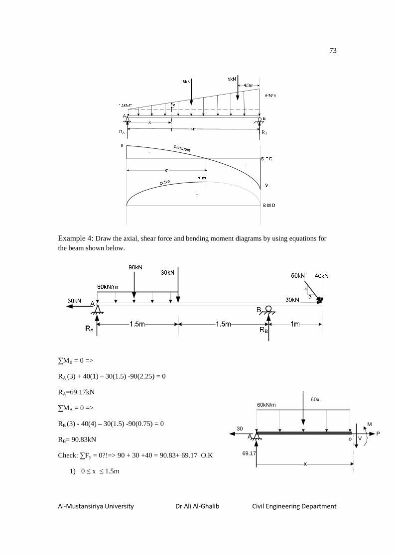
Example 4: Draw the axial, shear force and bending moment diagrams by using equations for the beam shown below.
∑MB = 0 =>
RA (3) + 40(1) – 30(1.5) -90(2.25) = 0
RA=69.17kN
∑MA = 0 =>
RB (3) - 40(4) – 30(1.5) -90(0.75) = 0
RB= 90.83kN
Check: ∑Fy = 0?!=> 90 + 30 +40 = 90.83+ 69.17 O.K
1) 0 ≤ x ≤ 1.5m
A
69.17
x
V
M
60kN/m
30P
60x
o

74
Al-Mustansiriya University Dr Ali Al-Ghalib Civil Engineering Department
∑Fx = 0 => P = 30
∑Fy = 0 => V = 69.17-60x
∑Mo = 0 =>
( + 60n�2 − 69.17n = 0
( = 69.17n − 30n�
2) 1.5m ≤ x ≤ 3m ∑Fx = 0 => P = 30
∑Fy = 0 => V +30 - 69.17 + 90 = 0; V = -50.83
∑Mo = 0 =>
M + 30(x-1.5) + 90(x-0.75) – 69.17(x) = 0
( = 112.5 − 50.83n
3) 3m ≤ x ≤ 4m
∑Fx = 0 => P = 30
∑Fy = 0 => V +90 + 30 - 69.17 – 90.83 = 0; V = 40
∑Mo = 0 =>
M + 30(x-1.5) + 90(x-0.75) – 69.17(x) -90.83(x-3) = 0
( = 40n − 160
A
69.17
x
V
M
60kN/m
30P
9030
o
A
69.17
x
V
60kN/m
30
9030
o
M
P
90.83
B
1.5m 1.5m

75
Al-Mustansiriya University Dr Ali Al-Ghalib Civil Engineering Department
Shear and moment diagrams by summation approach
Upward load +
Downward load -
For the element ∆x ∑Fy = 0 + (V+∆V) - p(x). ∆x - V = 0 ∆�∆n = �6n7
lim∆�→3∆�∆n = !Ì!n = �6n7
!Ì!n = �6n7………… . . 617 ∑MA = 0 (M + ∆M) – M –V. ∆x - p(x) ∆x(∆x/2) = 0 ∆(∆n = � − �6n7 ∆n2

76
Al-Mustansiriya University Dr Ali Al-Ghalib Civil Engineering Department
lim∆�→3∆(∆n = lim∆�→3� − lim∆�→3 �6n7
∆n2
!(!n = �6n7………… . . 627 From equation (2): !�(!n� = !�
!n
!�(!n� = �6n7…………637 Or, in opposite way:
From equation (1): dV = p(x) dx, hence; �6n7 = m �6n7!n ����3
That means the shear force at the section equals the summation (area) of all normal loadings that exists on one side of the section.
Also, from equation (2): dM = V(x) dx, hence; (6n7 = m �6n7!n ����3
That means the bending moment at the section equals the summation (area) of all shear forces that exists on one side of the section.
Examples
1.

77
Al-Mustansiriya University Dr Ali Al-Ghalib Civil Engineering Department
General notes on drawing the axial, shear and bendi ng moment diagrams
• Start drawing each diagram from the origin point, at the left hand side. The plot must end at the zero ordinate, at the right hand side.
• Any concentrated horizontal (axial) force to the right hand side makes a vertical downward jump with its magnitude in the axial force diagram, and vice versa.
• Any concentrated upward vertical (shear) force makes a vertical upward jump with its magnitude in the shear force diagram, and vice versa.
• Any concentrated clockwise bending moment makes a vertical upward jump with its magnitude in the bending moment diagram, and vice versa.
• When the loading diagram consists only of concentrated normal loads, the shear diagram will be of constant functions and the moment diagram will be of linear variation.
• When the loading diagram consists only of uniformly distributed loads, the shear diagram will be of linear functions and the moment diagram will be of second order variation.
• When the loading diagram consists only of linearly varying loads, the shear diagram will be of second order functions and the moment diagram will be of third order variation.
• The point of zero shear force represents a maximum bending moment point. 2.

78
Al-Mustansiriya University Dr Ali Al-Ghalib Civil Engineering Department
3.
4.

79
Al-Mustansiriya University Dr Ali Al-Ghalib Civil Engineering Department
5.
S.F.D
wkN/m
L
wL/2_
wL/2
wL2/3
2nd
order
wL/2L/3
_B.M.D
wL2/3
3rd
order
6.

80
Al-Mustansiriya University Dr Ali Al-Ghalib Civil Engineering Department
7.
Cuboid Parabola
Line
ar
8.

81
Al-Mustansiriya University Dr Ali Al-Ghalib Civil Engineering Department
Solution of example 8 by equations:
0 ≤ x ≤ 3
∑Fy =0; V= +450 (constant)
∑M0 =0; M= +450x (linear)
3 ≤ x ≤ 6
∑Fy =0; V= +450-300(x-3) (linear)
@x=3; V=450
@x=6; V=-450
∑M0 =0; M= +450x - 300/2(x-3)2(parabola)
@x=3; M=1350
@x=6; M=1350
@x=4.5; M=2025-337.5=1687.5
6 ≤ x≤ 9
∑Fy =0; V= +450+1350-300(x-3); V= 1800-300(x-3) (linear)
@x=6; V=900
@x=9; V=0
∑M0 =0; M= +450x +1350(x-6) - 300/2(x-3)2(parabola)
@x=6; M=1350
@x=9; M= 2700
82
Al-Mustansiriya University Dr Ali Al-Ghalib Civil Engineering Department
9.
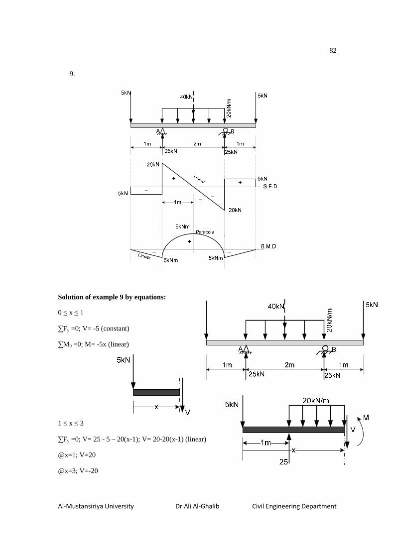
Solution of example 9 by equations:
0 ≤ x ≤ 1
∑Fy =0; V= -5 (constant)
∑M0 =0; M= -5x (linear)
1 ≤ x ≤ 3
∑Fy =0; V= 25 - 5 – 20(x-1); V= 20-20(x-1) (linear)
@x=1; V=20
@x=3; V=-20

83
Al-Mustansiriya University Dr Ali Al-Ghalib Civil Engineering Department
∑M0 =0; M= -5x- 20/2(x-1)2 +25(x-1) (parabola)
@x=1; M=-5
@x=3; M=-5
3 ≤ x ≤ 4
∑Fy =0; V= 25 + 25 -5-40; V= +5 (constant)
∑M0 =0; M= 25(x-1) +25(x-3) -5x-40(x-2) (linear)
10. Draw the SFD and BMD for the beam AC. Also, draw the deflected shape of the beam,
and show the point of contra flexure. Determine the maximum positive bending moment and find its location.
∑MB = 0
Rc (6) + 80 + 30(1.5) = 144(2);
Rc =27.2kN.
∑Fy = 0
RB + 27.2 -30 – 144 = 0;
RB = 146.8kN.
To find the position of zero shear point, take a free body diagram for the beam segment exists to the right of a section passes through the zero shear point, as shown below:
= = �
y=8x.
From the equilibrium equation:
∑Fy = 0; find x, as:
27.2 − 8n�2 = 0
xV=0
M
y
Rc
o

84
Al-Mustansiriya University Dr Ali Al-Ghalib Civil Engineering Department
x=2.61m.
∑Mo = 0;
( = 27.2(2.61) − 8 ∗ 2.61 ∗ 2.61 ∗ 2.612 ∗ 3
M=47.3kN.m
10kN/m
AB
C
48kN/m
80kN.m
3m 6m
-30
116.8
-27.2
SFD
BMD
__
+
x
Parabola
linear
-45
-125
Mmax
+
__
cubic
Parabola

85
Al-Mustansiriya University Dr Ali Al-Ghalib Civil Engineering Department
11. For the beam loaded as shown below, plot the shear and bending moment diagrams. Determine the magnitude of the maximum positive bending moment and find its location.

86
Al-Mustansiriya University Dr Ali Al-Ghalib Civil Engineering Department
To find the location of zero shear point, take the free body diagram of the section shown below:
2003 = gn
y=66.66x.
From the equilibrium equation ∑Fy = 0, find the value of x, as:
400 = 200n + 66.66n�2
33.33n� + 200n − 400 = 0
n = −200 ∓ Ê40000 + 4(33.33)(400)2(33.33)
x=1.583m
In order to find the maximum positive moment, use the following equilibrium equation:
∑Mo = 0;
(8B� = 400(1.583) − 200(1.583)(1.5832 7 − 66.6661.583761.5832 761.5833 7 Mmax=338.3N.m

87
Al-Mustansiriya University Dr Ali Al-Ghalib Civil Engineering Department
12. The overhanging beam AC supports a uniform load of intensity (w). Determine the value of x1 in terms of L such that the maximum positive bending moment equals the maximum negative bending moment.
∑MB=0;
@�j = ^(j + n�) ∗ [j − j + n�2 ] @�j = 2 (j + n�) ∗ (j − n�)
@� = 2j (j� − n��)�
(Î(n) = X�k (j� − n��)n − X�#�
!(!n = 2j (j� − n��) − ^n = 0
n = j� − n��2j
(8B�Î = X�k (j� − n��) ∗ k#L�#�k = X k 6j� − n��7�
(8B�L = ^n��2
Find the value of x1 when M+max= M-
max:
^4j (j� − n��)� = ^n��2
(j� − n��)�2j� = n��

88
Al-Mustansiriya University Dr Ali Al-Ghalib Civil Engineering Department
Take the square root of both sides of the equation,
(j� − n��)√2j = n�
n�� + 1.414jn� − j� = 0
n� = −1.414j ∓ √2j + 4j�2 = −1.414j + 2.45j2 = 0.518j

89
Al-Mustansiriya University Dr Ali Al-Ghalib Civil Engineering Department
Homework
1. The bending moment diagram of a beam is shown in the figure below. Construct the corresponding shear force and vertical loading diagrams.(Ans. Reaction at right-hand end= 100N)
2. Determine the shear force V and bending moment M at the midpoint C of the simple beam AB shown in the figure.(Ans. Vc=-0.9375kN; Mc=4.125kNm)
3. A simply supported beam AB supports a linearly distributed load (see figure). The intensity of the load varies linearly from50kN/m at support A to 25kN/m at support B. Construct the shear force and bending moment diagrams of the beam.(Ans. Vmidspan=-4.167kN; Mmidspan=75kNm)

90
Al-Mustansiriya University Dr Ali Al-Ghalib Civil Engineering Department
4. An overhanging beam AC carries a linearly varying load as shown below. Determine the position and the magnitude of the maximum positive bending moment. (Ans. Mmax=310Nm at x=2.12m from point A)
5. Write the shear force and bending moment equations at any point of the simply supported beam shown below. Plot the corresponding diagrams.(Ans. Mmax=12000Nm)
AB
C
1000N/m
1m 2m

91
Al-Mustansiriya University Dr Ali Al-Ghalib Civil Engineering Department
Chapter Five: Pure Bending of Beams
Pure bending refers to flexure of a beam under a constant bending moment. Therefore, pure bending occurs only in regions of a beam where the shear force is zero, as shown in the Figure 1. However, nonuniform bending refers to flexure in the presence of shear forces, which means that the bending moment changes as we move along the axis of the beam (Figure 2).
Figure 1: Simple beam in pure bending (M = M1)
Figure 2: Simple beam with central region in pure bending and end regions in nonuniform bending

92
Al-Mustansiriya University Dr Ali Al-Ghalib Civil Engineering Department
Curvature of a beam
When loads are applied to a beam, its longitudinal axis is deformed into a curve, as illustrated in Figure 3. The resulting strains and stresses in the beam are directly related to the curvature of the deflection curve.
Curvature is a measure of how sharply a beam is curved (bent). If the load on a beam is small, the beam will be nearly straight, the radius of curvature will be very large, and the curvature will be very small. If the load is increased, the amount of bending will increase - the radius of curvature will become smaller, and the curvature will become larger.
Figure 3: Bending of a cantilever beam
To point up the idea of curvature, the two points (m1 and m2) are located on the deflection curve. Point m1 is chosen at an arbitrary distance x from the y axis and point m2 is located at small distance ds further along the curve. At each of these points, a line normal to the tangent to the deflection curve is drawn. These normals intersect at point O’, which is the center of curvature of the deflection curve (Figure 4).
The distance O’m1 from the centre of curvature to the curve is called the radius of curvature ρ (Greek letter rho), and the curvature κ (Greek letter kappa) is defined as the reciprocal of the radius of curvature. Therefore,
Ï = 1¦
Figure 4: Curvature of a bent beam

93
Al-Mustansiriya University Dr Ali Al-Ghalib Civil Engineering Department
Bending formula
Basic assumptions
1. A plane section before bending remains plane after bending. 2. The material is linear elastic (i.e. follows Hooke’s law). 3. The modulus of elasticity (E) is same in both tension and compression.
Figure 5: Deformations of a beam in pure bending: (a) side view of beam, (b) deformed beam

94
Al-Mustansiriya University Dr Ali Al-Ghalib Civil Engineering Department
Figure 6: Behavior of a beam in bending
J� = ¦!§
ff ′ = g!§
i = ff′J� =
g¦
Since the material is linear elastic:
� = lg¦ ⋯⋯617
The normal bending stress is varying linearly from zero at NA to a maximum value at extreme fibers (mp and nq).

95
Al-Mustansiriya University Dr Ali Al-Ghalib Civil Engineering Department
Figure 7: Distribution of bending stress in a beam
( = r �!.gBCAB
( = r l. g¦ !.g
BCAB
( = l¦ r g�!BCAB
( = l¦ ∗Ð5�
¦ = lÐ( ⋯⋯ 627
And from equation (1):
¦ = lg� ⋯⋯617
lg� = lÐ
(
� = (gÐ ⋯⋯Ñ`\!b\�f]eJ[c<
In symmetrical sections about x-axis, the maximum bending stress is:

96
Al-Mustansiriya University Dr Ali Al-Ghalib Civil Engineering Department
�8B� = (�Ð ⋯⋯Ñ`\!b\�f]eJ[c<
In unsymmetrical sections about x-axis, the maximum bending stresses are:
C1
C2
��78B� = (�1Ð ⋯⋯Ñ`\!b\�f]eJ[c<
��78B� = (�2Ð ⋯⋯Ñ`\!b\�f]eJ[c<
Elastic section modulus
�78B� = Ò?Ó =Ò�
Where:
Ô = Ð�
For a rectangular section:
Ð5� = �ℎH12
Ô = Ð5�� = �ℎ�6
h
b
NA

97
Al-Mustansiriya University Dr Ali Al-Ghalib Civil Engineering Department
For a circular section:
Ð5� = R4 @
Ô = Ð5�� = R4 @H
Some useful moments of inertia
Triangle
Ð5� = �V4H=
Semicircle
� = R8 @
Ð� = Ð� � Õ4@3RÖ�
� = 0.11@
RNA
h
b
NA
h/3

98
Al-Mustansiriya University Dr Ali Al-Ghalib Civil Engineering Department
Example 1: The cantilever beam, shown in the figure below, has 2.0m span and carries a uniformly distributed load of magnitude 2kN/m and a concentrated vertical load of 10kN. Determine the bending stress distribution at the critical section.
Solution: a critical section is the section where the maximum bending moment and consequently the maximum bending stress occurs.
In order to find the location of NA, y1:
g1 = ∑ g∑
g1 = 20062076107 � 1806207611072006207 � 1806207 = 57.37JJ
Ð5� ='6Ð� �!�7
Ð5� = 2006207H12 � 2006207647.37)� + 20(180)H
12+ 20(180)(110 − 57.37)�= 2.88 ∗ 10|JJ
��)8B� = (�1Ð = 24 ∗ 10=IJJ ∗ 6200 − 57.377JJ
2.88 ∗ 10|JJ = 118.85(�<6�`\ab]\7
��78B� = (�2Ð = 24 ∗ 10=IJJ ∗ 657.377JJ
2.88 ∗ 10|JJ = 47.81(�<6�]J�e`aab]\7
24kN.m
14kN
2kN/m10kN
10kN
14kN
-
24kNm
-

99
Al-Mustansiriya University Dr Ali Al-Ghalib Civil Engineering Department
Stress blocks at the critical section

100
Al-Mustansiriya University Dr Ali Al-Ghalib Civil Engineering Department
Example 2: Determine the maximum tensile and compressive bending stresses developed in the overhanging beam shown below.
Section
Solution: from the bending moment diagram, there appear two critical sections because there are a maximum positive moment and a maximum negative moment.
In order to find the location of NA, y1:
g1 = ∑ g∑
g1 = 400(600)(300) − [R(100)�(300)] − 100(100)(550)400(600) − R(100)� − 100(100) = 287.4JJ
Ð5� = '(Ð� + !�)
Ð5� = 400(600)H12 + 400(600)(300 − 287.4)� − 2 ∗ ²R(100)
8 + R(100)�2 (300 − 287.4)�³
− ²100(100)H12 + 100(100)(550 − 287.4)�³ = 6.46 ∗ 10�JJ
200m
m20
0mm
200m
m
++
100
150 150100
y1
NA
12kN/m
6m 2m
AB
96kN
64kN32kN
2.67m
32 24
40
SFD
BMD
24
42.67
+ +
+
_
-

101
Al-Mustansiriya University Dr Ali Al-Ghalib Civil Engineering Department
Positive bending moment zone:
��)8B� = (�1Ð = 42.67 ∗ 10=IJJ ∗ 6600 − 287.4)JJ6.46 ∗ 10�JJ = 2(�<
��78B� = (�2Ð = 42.67 ∗ 10=IJJ ∗ 6287.4)JJ6.46 ∗ 10�JJ = 1.9(�<
Negative bending moment zone:
��78B� = (�2Ð = 24 ∗ 10=IJJ ∗ 6287.4)JJ6.46 ∗ 10�JJ = 1.07(�<
��78B� = (�1Ð = 24 ∗ 10=IJJ ∗ 6600 − 287.4)JJ6.46 ∗ 10�JJ = 1.16(�<

102
Al-Mustansiriya University Dr Ali Al-Ghalib Civil Engineering Department
Example 3: When two concentrated forces were applied at a W460 x 82 steel beam as shown in figure, an elongation of 0.12mm was observed between the gauge points A and B. What was the magnitude of the applied forces? Take E=200GPa and I= 371x106mm4.
Solution:
i�����8 = i�) = ∆�)j�) = 0.12JJ200JJ = 0.0006
��) = i�) ∗ l = 0.0006 ∗ 200 ∗ 10H= 120(�<
Bending formula:
��) = ( ∗ �Ð => 120 = ( ∗ 62307JJ
371 ∗ 10=JJ
120 = 62000 ∗ �7 ∗ 62307JJ371 ∗ 10=JJ => � = 96783I = 96.8NI
P P
P P
P
P
+
-
+
SFD
BMD
2m 2m2m
2*P
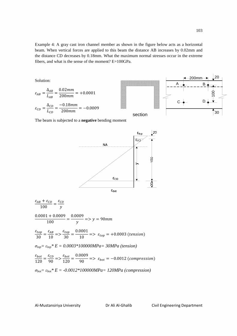
103
Al-Mustansiriya University Dr Ali Al-Ghalib Civil Engineering Department
Example 4: A gray cast iron channel member as shown in the figure below acts as a horizontal beam. When vertical forces are applied to this beam the distance AB increases by 0.02mm and the distance CD decreases by 0.18mm. What the maximum normal stresses occur in the extreme fibers, and what is the sense of the moment? E=100GPa.
Solution:
i�) = ∆�)j�) = 0.02JJ200JJ = +0.0001
i?x = ∆?xj?x = −0.18JJ200JJ = −0.0009
The beam is subjected to a negative bending moment
i�) + i?x100 = i?xg
0.0001 + 0.0009100 = 0.0009g => g = 90JJ
i���30 = i�)10 => i���30 = 0.000110 => i��� = �0.00036T`\ab]\7 σtop= εtop* E = 0.0003*100000MPa= 30MPa (tension)
i���120 =i?x90 => i���120 =
0.000990 => i��� = −0.00126d]J�e`aab]\7
σbot= εbot* E = -0.0012*100000MPa= 120MPa (compression)
200mm
100
20
30
A
DC
B
section

104
Al-Mustansiriya University Dr Ali Al-Ghalib Civil Engineering Department
Beams of Two Materials
Stress Distribution in Composite Sections (Method o f Transformed section)
Same assumptions used in deriving the bending formula are valid in the composite sections.
Modular ratio \ = q¯q#
Reinforcing steel
Concrete
………..……
…..
wood
steel

105
Al-Mustansiriya University Dr Ali Al-Ghalib Civil Engineering Department
\′ = l�l�
Example: A composite beam is constructed from a wood beam (150mm x 250mm) and a steel reinforcing plate (10mm thick x 150mm wide), as shown in the figure below. If the beam is subjected to a positive bending moment of 30kN.m around its horizontal axis, determine the maximum stresses developed in steel and wood. Take Es=200GPa and Ew=10GPa.
25
0m
m1
0
y1
Solution: The first step in the analysis is to locate the neutral axis of the cross section.
Modular ratio \ = qsq× = �33
�3 = 20
��∗ = \. �� = 2061507 = 3000JJ
g1 = 30006107657 � 150625076135730006107 � 15062507 = 77JJ
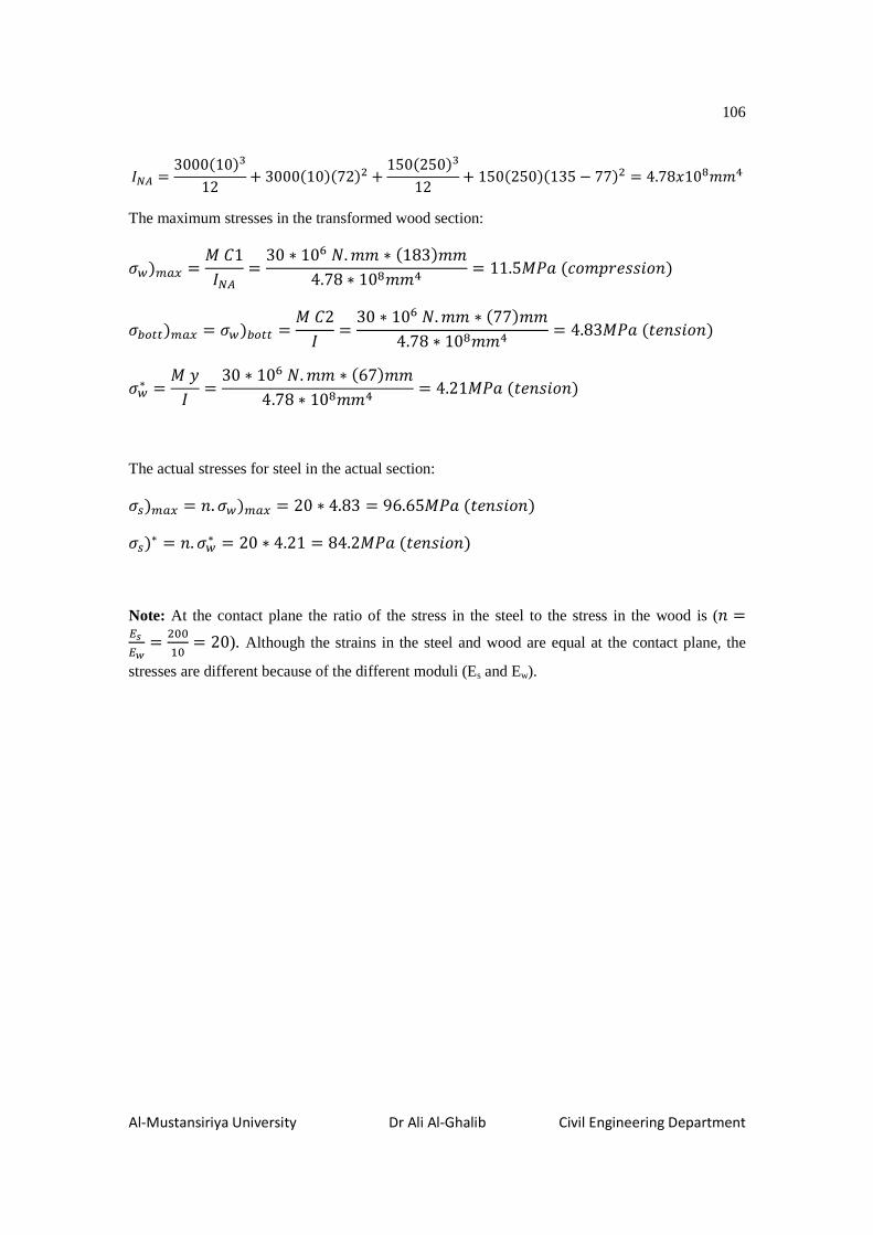
106
Al-Mustansiriya University Dr Ali Al-Ghalib Civil Engineering Department
Ð5� = 3000(10)H12 + 3000(10)(72)� + 150(250)H
12 + 150(250)(135 − 77)� = 4.78n10JJ
The maximum stresses in the transformed wood section:
�X)8B� = (�1Ð5� = 30 ∗ 10=I.JJ ∗ 61837JJ4.78 ∗ 10JJ = 11.5(�<6d]J�e`aab]\7
�����78B� = �X7���� = (�2Ð = 30 ∗ 10=I.JJ ∗ 6777JJ4.78 ∗ 10JJ = 4.83(�<6T`\ab]\7
�X∗ = (gÐ = 30 ∗ 10=I.JJ ∗ 6677JJ4.78 ∗ 10JJ = 4.21(�<6T`\ab]\7
The actual stresses for steel in the actual section:
�w78B� = \. �X78B� = 20 ∗ 4.83 = 96.65(�<6T`\ab]\7 �w7∗ = \. �X∗ = 20 ∗ 4.21 = 84.2(�<6T`\ab]\7
Note: At the contact plane the ratio of the stress in the steel to the stress in the wood is (\ =qsq× = �33
�3 = 20). Although the strains in the steel and wood are equal at the contact plane, the
stresses are different because of the different moduli (Es and Ew).

107
Al-Mustansiriya University Dr Ali Al-Ghalib Civil Engineering Department
Example 2: Determine the maximum stress in concrete and steel for the reinforced concrete beam of the section shown below. The section is subjected to a positive bending moment of 70kN.m. Assume the modular ratio n=15. Compare the maximum stresses with the allowable stresses in both concrete and steel.
��
�..
��
�..
Solution: As the concrete under tension stresses is very weak, it will crack below the neutral surface (for the positive moment) and the steel rods will carry the entire tensile load, while the upper part of the concrete beam will carry the compressive load. That is to say, we consider the concrete area in the tension zone is negligible.
w = 2 ∗ R4 (30)� = 1413.7JJ�
\. w = 15 ∗ 1413.7 = 21206JJ�
To find the location of the NA:
The first moment of the compression area around the NA = the first moment of the tension area around the NA.
250* kd* kd/2 = 21206* (500-kd)
N!� + 169.65N! − 84823 = 0
kd=218.5mm
Ð5� = 250(218.5)H3 + 21206(500 − 218.5)� = 2.55 ∗ 10�JJ
��)8B� = (�1Ð5� = 70 ∗ 10=I.JJ ∗ 6218.57JJ
2.55 ∗ 10�JJ = 6.0(�<6d]J�e`aab]\7 < 0.45f�′= 0.45(21) = 9.45(�<
�w = \ ∗ (�2Ð5� = 15 ∗ 70 ∗ 10=I.JJ ∗ 6281.57JJ
2.55 ∗ 10�JJ = 115.9(�< < fw7B���X = 140(�<

108
Al-Mustansiriya University Dr Ali Al-Ghalib Civil Engineering Department
Example 3: A hollow rectangular reinforced concrete section is cast as shown in the figure below. The modular ratio n=10, and the maximum compressive stress in the concrete caused by positive bending moment is 7MPa. Determine the stress in the steel and the bending moment applied to the section.
Solution: We need first to transform the actual composite section to a concrete transformed section.
nAs= 10*3600 = 36000mm2
Now, we need to find the location of the neutral axis for the transformed section:
N! = 2 ∗ 100 ∗ N! ∗ M&� + 400 ∗ 120 ∗ 60 + 36000 ∗ 11202 ∗ 100 ∗ N! + 400 ∗ 120 + 36000
N! = 100N!� + 43200000200N! + 48000 + 36000
N!� + 840N! − 432000 = 0
N! = −840 + Ê840� + 4(432000)2 = 360JJ
Ð5� = 100 ∗ (360)H3 ∗ 2 + 400 ∗ (120)H
12 + 400(120)(300)� + 36000(760)�
Ð5� = 3.1 ∗ 10� + 5.76 ∗ 10| + 4.32 ∗ 10� + 2.08 ∗ 10�3 = 2.83 ∗ 10�3JJ
��) tp = ( ∗ N!Ð5� => 7 IJJ� = ( ∗ 360JJ2.83 ∗ 10�3JJ => ( = 550NI. J
�w = \ ∗ ( ∗ (1120 − N!)Ð5� = 10 ∗ 550 ∗ 10=I. JJ ∗ (1120 − 360)JJ2.83 ∗ 10�3JJ = 147.7(�<

109
Al-Mustansiriya University Dr Ali Al-Ghalib Civil Engineering Department
20% Q3: The reinforced concrete section of the T-shape shown in Fig.3 is subjected to a positive bending moment of 150kN.m.If the modular ratio n=10, determine the maximum compressive stress in the concrete and the stress in the steel.
Solution:
600mm
300mm
4 ɸ 25mm
w = I]. ]f�<ea ∗ R4 !� = 4 ∗ R4 (25)� = 1963.5JJ�
e`<]fTe<\af]eJ`!aT``cT]d]\de`T` = \ ∗ w = 10 ∗ 1963.5 = 19635JJ�
After making the transformed section (as shown in the figure above), obtain the position of N.A.
First moment of compression area about N.A = First moment of tension area about N.A.
600 ∗ 100 ∗ 6N! − 507 � 3006N! − 1007 ∗ 6N! − 10072 = 196356500 − N!7
150N!� � 3006N! − 1007 ∗ 6N! − 10072 = 196356500 − N!7
150N!� � 49635N! − 11317500 = 0
N!� + 330.9N! − 75450 = 0
N! = −330.9 + Ê330.9� + 4(75450)2 = 155JJ
Ð5� = 600 ∗ (100)H12 + 600 ∗ 100 ∗ (155 − 50)� + 300 ∗ (55)H
3 + 19635(500 − 155)�
600mm
500m
m10
0
kd
nAs
300mm
Transformed section
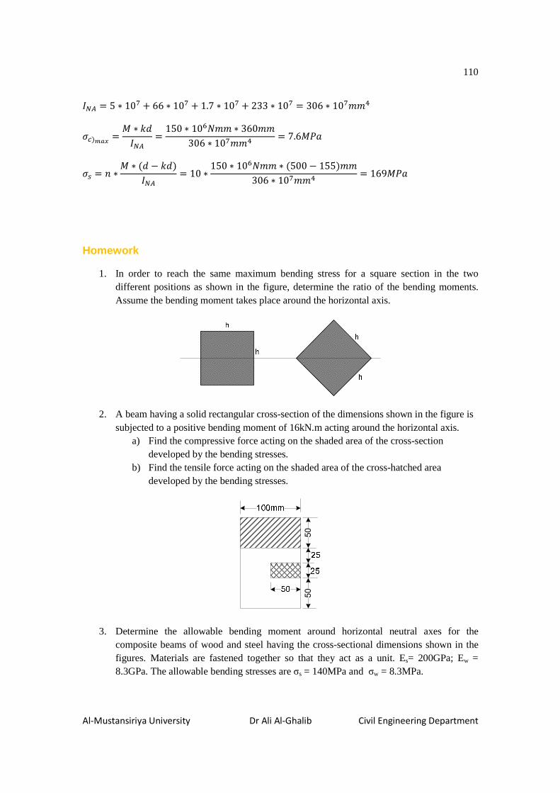
110
Al-Mustansiriya University Dr Ali Al-Ghalib Civil Engineering Department
Ð5� = 5 ∗ 10| + 66 ∗ 10| + 1.7 ∗ 10| + 233 ∗ 10| = 306 ∗ 10|JJ
��) tp = ( ∗ N!Ð5� = 150 ∗ 10=IJJ ∗ 360JJ306 ∗ 10|JJ = 7.6(�<
�w = \ ∗ ( ∗ (! − N!)Ð5� = 10 ∗ 150 ∗ 10=IJJ ∗ (500 − 155)JJ306 ∗ 10|JJ = 169(�<
Homework
1. In order to reach the same maximum bending stress for a square section in the two different positions as shown in the figure, determine the ratio of the bending moments. Assume the bending moment takes place around the horizontal axis.
2. A beam having a solid rectangular cross-section of the dimensions shown in the figure is subjected to a positive bending moment of 16kN.m acting around the horizontal axis.
a) Find the compressive force acting on the shaded area of the cross-section developed by the bending stresses.
b) Find the tensile force acting on the shaded area of the cross-hatched area developed by the bending stresses.
50
50
3. Determine the allowable bending moment around horizontal neutral axes for the composite beams of wood and steel having the cross-sectional dimensions shown in the figures. Materials are fastened together so that they act as a unit. Es= 200GPa; Ew = 8.3GPa. The allowable bending stresses are σs = 140MPa and σw = 8.3MPa.

111
Al-Mustansiriya University Dr Ali Al-Ghalib Civil Engineering Department
4. A simple beam of span length 3.2m carries a uniform load of intensity 48kN/m. The cross section of the beam is a hollow box with wood flanges and steel side plates, as shown in the figure. The wood flanges are 75mm by 100mm in cross section, and the steel plates are 300 mm deep. What is the required thickness t of the steel plates if the allowable stresses are 120MPa for the steel and 6.5MPa for the wood? (Assume that the moduli of elasticity for the steel and wood are 210GPa and 10GPa, respectively, and disregard the weight of the beam.) Answer: tmin=15mm.

112
Al-Mustansiriya University Dr Ali Al-Ghalib Civil Engineering Department
Chapter Six: Shearing Stresses in Beams
In a beam loaded by transverse forces acting perpendicular to the axis of the beam, as shown in the figure below, not only are bending stresses generated parallel to the axis of the beam but shearing stresses also act over cross sections of the beam perpendicular to the axis of the beam.
A Bdx
jjb
dd
b j
ff
b
h
y1
j h
f g
Neutral axis
FA FBdF
dx
Vx
Mx

113
Al-Mustansiriya University Dr Ali Al-Ghalib Civil Engineering Department
Assume: MB>MA; σB>σA; FB>FA
dF = FB-FA
!� = m �. ! −BCABÙFVÚ m �. !BCABB�&A
!� = r() . gÐ5� ! − r(�. gÐ5� !
!� = () −(�Ð5� rg. !
Let: MB = MA + dM
!� = (� � !( −(�Ð5� rg. !
Divide both sides by dx:
!�!n = !(/!nÐ5� r g. !
Let: q= dF/dx = shear flow, which is the shear force per unit length.
� = !(!n
Û = r g! = gÜBCABB�&AB�&A = fbeaTJ]J`\T]f<e`<<�][TI
_ = �ÛÐ5�
Then, the shear stress can be given as:
dF

114
Al-Mustansiriya University Dr Ali Al-Ghalib Civil Engineering Department
= &�&Ý� = _� = �ÛÐ5��
Q is the first moment of area separated by the fibe r about NA
Q= 100*30*85= 255000mm3
Or, alternatively:
Q=100*170*15= 255000mm3
The Shear Flow (q) would help to find the spacing between bolts, as follow:
Ô = �Ç
Where:
S= spacing between the bolts, and
F= allowable shearing force per bolt.
Example 1: The T shaped wooden beam of the cross-sectional dimensions given in the figure below transmits a vertical shear force of 3000N. Find the necessary spacing of the nails connected the two planks in order to make the beam acts as a unit. Assume that the allowable shearing force carried by each nail is 700N.
Solution:
Find the location of the NA:
g1 = 200(50)(25) + 50(200)(150)200(50) + 50(200) = 87.5JJ
Ð5� = 200(50)H12 + 200(50)(87.5 − 25)� + 50(200)H
12+ 50(200)(150 − 87.5)�= 1.135 ∗ 10JJ
Q = 200 (50) (87.5-25) = 625000mm3
b=100mm
h=20
0mm y1
Neutral axis
30mm
fiber
S
50m
m20
0mm
50
200x
NA
y1

115
Al-Mustansiriya University Dr Ali Al-Ghalib Civil Engineering Department
Or, Q =50 (200) (150-87.5) = 625000mm3
_ = �ÛÐ5� = 3000I ∗ 625000JJH
1.135 ∗ 10JJ = 16.51I/JJ
Ô�<db\��`T^``\\<bca, Ô = �_ = 700I
16.51I/JJ = 42.4JJ
Practically, use nails spacing @ 40mm c/c.
Solution for alternative arrangement of planks:
Nails between planks 1 and 2:
Q= 25(50) (87.5-25) = 78125mm3
_ = �ÛÐ5� = 3000I ∗ 78125JJH
1.135 ∗ 10JJ = 2.06I/JJ
Ô�<db\��`T^``\\<bca, Ô = �_ = 700I
2.06I/JJ = 340JJ
Nails between planks 2 and 3:
Q = 75 (50) (87.5-25) = 234375mm3
_ = �ÛÐ5� = 3000I ∗ 234375JJH
1.135 ∗ 10JJ = 6.19I/JJ
Ô�<db\��`T^``\\<bca, Ô = �_ = 700I
6.19I/JJ = 113JJ
50m
m20
0mm
50
NA
87.5
150 2525
1
3
2

116
Al-Mustansiriya University Dr Ali Al-Ghalib Civil Engineering Department
Example 2: A simply supported beam of 6.0m span supports a uniformly distributed load of intensity of 3.0kN/m, and has the cross-sectional dimensions shown below. Determine the necessary spacing between 10mm vertical screws whereby each screw can transmit a shear force of 2.0kN. Take INA = 2.36x10⁻³m4
Solution:
First moment of area (shaded area) about NA, Û = ∑ gÞ Q = 200(50) (225) +2 (50) (100) (200) = 4.25* 106mm3
_ = �ÛÐ5� = 9000I ∗ 4.25 ∗ 10=JJH
2.36 ∗ 10�JJ = 16.2I/JJ
Near the supports:
Ô = �_ = 2000I16.2I/JJ = 123.5JJ
Similar calculation when V=4.5kN, to cover the mid span zone:
_ = �ÛÐ5� = 4500I ∗ 4.25 ∗ 10=JJH
2.36 ∗ 10�JJ = 8.1I/JJ
Ô = �_ = 2000I8.1I/JJ = 247JJ
The shearing stress formula for a rectangular cross-section:
3kN/m
6m
9kN
9kN
+-1.5m
3m
SFD
200mm50 50
500
100
NA
100
50
section
aa

117
Al-Mustansiriya University Dr Ali Al-Ghalib Civil Engineering Department
= �ßÓ�z�
� = �[� �V� − g�� ∗ �� �V� + g��]Ð5��
� = �2Ð5� Y6
ℎ27� − g��]
To find the maximum shear stress,
!!g� =
�2Ð5� �0 − 2g� � = 0;g� = 0
½¾¹¿ = à ∗ áÁ ∗ âãä
½¾¹¿ = à ∗ áÁ ∗ ºá»
ÄÁ= »àÁºá = »
Áàä
If ½¹åæ = àä;
½¾¹¿ = Ä. ç½¹åæ
Volume of shear stresses block= 2/3*τmax*b*h
�]c[J` = 23 Õ
32��ℎÖℎ� = �
b
h
y1
Neutral axis
fiber

118
Al-Mustansiriya University Dr Ali Al-Ghalib Civil Engineering Department
Example 1: Determine the shearing stresses at different levels of an I-section beam, which is loaded as shown in the figure below.
500kN
250kN 250kN
a
a
Solution:
Ð5� = 150(300)H12 − 138(276)H
12 = 95.7 ∗ 10=JJ
= �ÛÐ5��
�L� = 0, �`d<[a`Û = 0
�L�7Ù�BEFA = 250000 ∗ Y150 ∗ 12 ∗ 144]95.7 ∗ 10= ∗ 150 = 4.5(�<
�L�)XA� = 250000 ∗ [150 ∗ 12 ∗ 144]95.7 ∗ 10= ∗ 12 = 56.4(�<
HLH = 250000 ∗ [150 ∗ 12 ∗ 144 + 12 ∗ 12 ∗ 132]95.7 ∗ 10= ∗ 12 = 60.5(�<
L = 250000 ∗ [150 ∗ 12 ∗ 144 + 12 ∗ 138 ∗ 69]95.7 ∗ 10= ∗ 12 = 81.3(�<

119
Al-Mustansiriya University Dr Ali Al-Ghalib Civil Engineering Department
Example 2: A T-beam has cross-sectional dimensions shown in the figure below is subjected to a shear force V=68kN. Determine the maximum shear stress in the web of the beam.
g1 = 210 ∗ 20 ∗ 10 + 16 ∗ 280 ∗ 160210 ∗ 20 + 16 ∗ 280 = 87.42JJ
Ð5� = 210(20)H12 + 210 ∗ 20 ∗ (87.42 − 10)� + 16(280)H
12 + 16∗ 280 ∗ (160 − 87.42)� = 7.82 ∗ 10|JJ
= �ßÓ�z�
8B� = 5� = 68000 ∗ [16 ∗ 212.58 ∗ 106.29]7.82 ∗ 10| ∗ 16 = 19.64(�<
Example 3: A steel cantilever beam is made of two structural tee- section beams welded together as shown in the figure below. Determine the allowable safe load (P) that the beam can carry. The allowable stresses are: σ=150MPa in tension and compression, τ=100MPa in shear, and q=2000N/mm on the welded joint.
Solution: Find the position of the neutral axis.
g1 = �23(�2)(��.2)�2(�33)(��2)�33(�2)(�H|.2)�23(�2)�2(�33)�33(�2) = 135.2JJ
Determine the moment of inertia of the section about neutral axis.
210mm
300m
m
280
16mm
section
NA
y1
200mm
150
100
150
weld
25
25
section
y1
NA
25

120
Al-Mustansiriya University Dr Ali Al-Ghalib Civil Engineering Department
Ð5� = 1506257H12 � 15062576135.2 U 12.57� � 2562007H12 � 25620076135.2 U 1257�
� 2006257H12 � 20062576237.5 U 135.27� � 1.26 ∗ 10JJ
• The allowable force (P) based on the bending stresses:
� � (�Ð5�
�B���X � 150(�<, f]e�]T�T`\ab]\<\!d]J�e`aab]\
150(�< � 1000� ∗ 135.21.26 ∗ 10 �W � � 140NI
• The allowable force (P) based on the shearing stresses: V=P;
� �ÛÐ5��
5� � � ∗ Y200 ∗ 25 ∗ 102.3 � 25 ∗ 89.8 ∗ 44.9Z1.26 ∗ 10 ∗ 25 � 100(�< �W � � 514.5NI
• The allowable force (P) based on the shear flow in the welding joint:
_ � �ÛÐ5�
Q=200(25)(102.3)+25(125)(27.3)= 5.97*105mm3
_XA�& � � ∗ 5.97 ∗ 1021.26 ∗ 10 � 2000 �W � � 422.2NI
The safe allowable load Psafe= 140kN
Example: A wood box beam shown in the figure is constructed of two boards, each 180x40mm in cross section, that serve as flanges and two plywood webs, each 15mm thick. The total height of the beam is 280mm. The plywood is fastened to the flanges by wood screws having an allowable load in shear of F=800N each. If the shear force V acting on the cross section is 10.5kN, determine the maximum permissible longitudinal spacing (S) of the screws.
Solution:
Ð5� � 21062807H12 U 18062007H12 � 2.64 ∗ 10JJ

121
Al-Mustansiriya University Dr Ali Al-Ghalib Civil Engineering Department
Û � 12 (180 ∗ 40 ∗ 120) = 432000JJH
_ = �ÛÐ5�
_ = 10.5 ∗ 10H ∗ 4320002.64 ∗ 10 = 17.18IJJ
Ô = �_ = 80017.18 = 46.6JJ
For practical fabrication of the beam, use spacing between screws S=45mm.
Example: A beam is loaded so that the moment diagram of it varies as shown in the figure.
a. Find the maximum longitudinal shearing force in the 12mm diameter bolts spaced 300mm apart.
b. Find the maximum shearing stress in the glued joint.
Solution: Find the position of the neutral axis
g1 = 200(50)(25) + 100(150)(125)200(50) + 100(150) = 85JJ
Determine the moment of inertia of the section about neutral axis
Ð5� = 200(50)H12 + 200(50)(85 − 25)� + 100(150)H
12 + 100(150)(125 − 85)� = 9 ∗ 10|JJ

122
Al-Mustansiriya University Dr Ali Al-Ghalib Civil Engineering Department
a) Find Q @ the red fiber, which represents Q for the bolt
Q= 100(50) (-60) +150(50) (40) =-300000+300000=0
q=0
b) Find Q @ the glued joint
Q=200(50) (60) =600000mm3
Or: Q=100(150) (40) =600000mm3
� �ÛÐ5��
F�«A � 5000 ∗ 6000009 ∗ 10| ∗ 100 = 0.333(�<

123
Al-Mustansiriya University Dr Ali Al-Ghalib Civil Engineering Department
% Q3: A double T beam is constructed of three wood boards, as shown in the figure. The flange and the webs are joined together by screws of an allowable shear force F=1200N per screw.
a) Calculate the maximum permissible longitudinal spacing of the screws. b) Calculate the maximum bending stress in the beam section.
500mm
100 100
2m 2m
12kN
x
NA6kN
6kN
S.F.D+
-
+
12kNm
B.M.D
Solution: In order to find the location of NA, y1:
g1 = ∑ g∑
g1 = 500(100)(50) + 2[300(100)(250)]500(100) + 2(300)(100) = 159JJ
Ð5� = '(Ð� + !�)
Ð5� = 500(100)H12 + 500(100)(159 − 50)� + 2
∗ ²100(300)H12 + 100(300)(250 − 159)�³ = 1.58 ∗ 10�JJ
a) V=6kN

124
Al-Mustansiriya University Dr Ali Al-Ghalib Civil Engineering Department
Û � 12 [500(100)(159 − 50)] = 2725000JJH
_ = �ÛÐ5� � 6000I ∗ 2725000JJH1.58 ∗ 10�JJ = 10.34I/JJ
Ô = �_ = 1200I�3.H 588= 116JJ
b) M=12kN.m
��)8B� = (��Ð � 12 ∗ 10=IJJ ∗ 159JJ1.58 ∗ 10�JJ = 1.2(�< ��78B� � (��Ð � 12 ∗ 10=IJJ ∗ (400 − 159)JJ1.58 ∗ 10�JJ = 1.8(�<

125
Al-Mustansiriya University Dr Ali Al-Ghalib Civil Engineering Department
Homework
1. Two wood box beams (beams A and B) have the same outside dimensions (200mm x 360mm) and the same thickness (t=20mm) throughout, as shown in the figure on the next page. Both beams are formed by nailing, with each nail having an allowable shear load of 250N. The beams are designed for a shear force V=3.2kN.
a) What is the maximum longitudinal spacing A for the nails in beam A? s=78.3mm. b) What is the maximum longitudinal spacing B for the nails in beam B? s=97.9mm. c) Which beam is more efficient in resisting the shear force?
2. A cast-iron beam has the cross-sectional dimensions shown in the figure. If the allowable
stresses are 50MPa in tension, 205MPa in compression and 55MPa in shear, what are the maximum allowable shear and the maximum allowable bending moment in this beam? Confine your calculations at the holes at section a-a. Ans: 417kN, 39.6 kN.m.
3. A steel welded box girder having the dimensions shown in the figure transmits a vertical shear force V=1500kN. Determine the shearing stresses at the sections a, b and c. For the section, I=15x109mm4.

126
Al-Mustansiriya University Dr Ali Al-Ghalib Civil Engineering Department
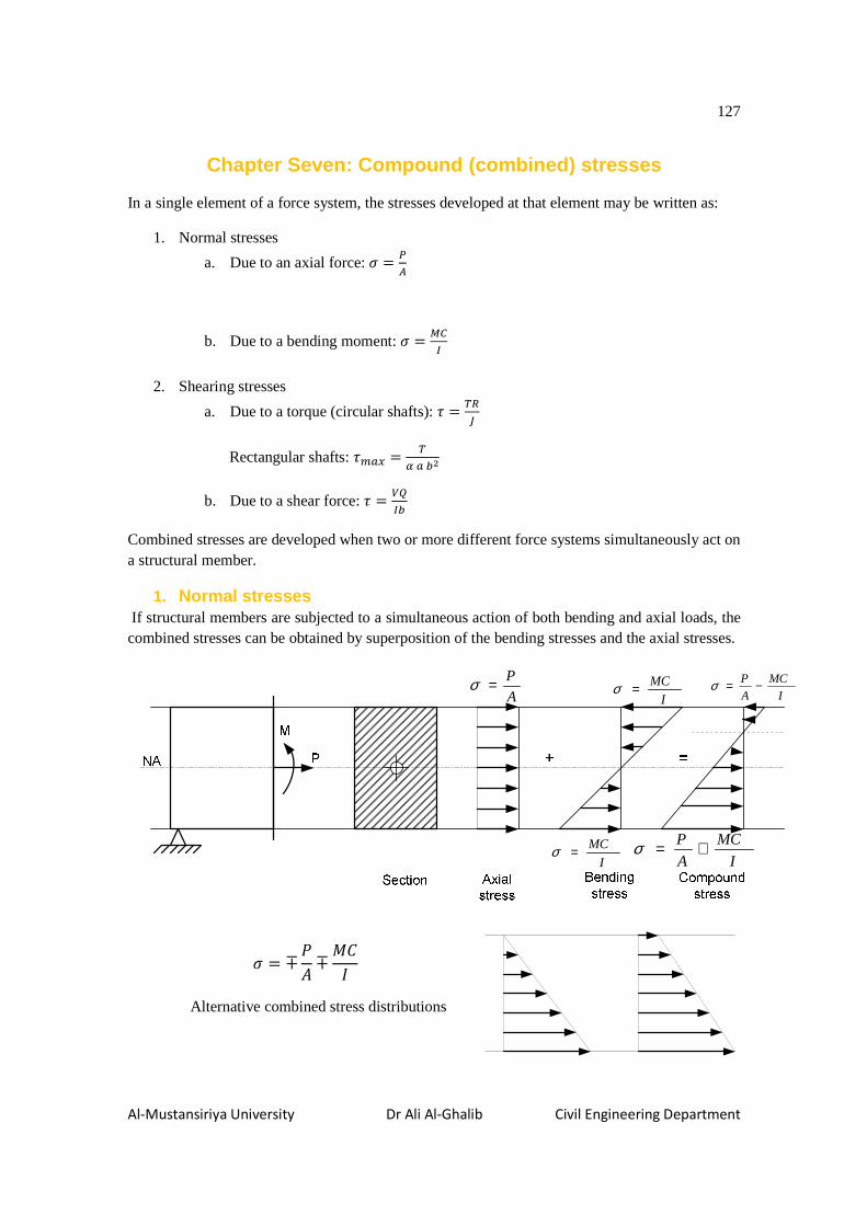
127
Al-Mustansiriya University Dr Ali Al-Ghalib Civil Engineering Department
Chapter Seven: Compound (combined) stresses
In a single element of a force system, the stresses developed at that element may be written as:
1. Normal stresses
a. Due to an axial force: � � P�
b. Due to a bending moment: � � Ò?Ó
2. Shearing stresses
a. Due to a torque (circular shafts): � y�ª
Rectangular shafts: 8B� � yèB�# b. Due to a shear force: � �ßÓ�
Combined stresses are developed when two or more different force systems simultaneously act on a structural member.
1. Normal stresses If structural members are subjected to a simultaneous action of both bending and axial loads, the combined stresses can be obtained by superposition of the bending stresses and the axial stresses.
I
MC
A
P −=σ
I
MC
A
P +=σ
I
MC=σ
I
MC=σ
A
P=σ
� � ∓� ∓(�Ð
Alternative combined stress distributions

128
Al-Mustansiriya University Dr Ali Al-Ghalib Civil Engineering Department
Example: A 50mmx75mm, 1.5m bar is loaded as shown in the figure below. Determine the maximum tensile and compressive stresses acting normal to the section through the beam.
75m
m
Solution:
Axial stress:
�B�DB� � P� � �233323∗|2 = 6.67(�<
Bending stresses:
��AE&DEF = (�Ð = 1.013 ∗ 10= ∗ 37.523∗|24��= 21.6(�<
Using the superposition principal:
���� = + � − (�Ð = 6.67 − 21.6 = −14.93(�<
���� = + � + (�Р= 6.67 + 21.6 = +28.27(�<
MPa67.6=σ MPa6.21=σ
MPa6.21=σ
MPa93.14=σ
MPa27.28=σ
375mm 1125
3.6kN
25kN25kN
2.7kN 0.9kN
2.7kN
0.9kN
SFD+
-
+BMD
1.013kN.m

129
Al-Mustansiriya University Dr Ali Al-Ghalib Civil Engineering Department
From the symmetry of the triangles:
g14.93 = 7514.93 + 28.27 => g = 25.92JJ
� = 14.93 ∗ 25.922 ∗ 50 ∗ 10LH = 9.68NI
� = 28.27 ∗ (75 − 25.92)2 ∗ 50 ∗ 10LH = 34.68NI
The axial force: P = T-C= 34.68-9.68= 25kN
M = (T * d1) + (C * d2)
( = 34.68NI ∗ 32.721000 J + 9.68NI ∗ 17.281000 J = 1.30NI. J
M – P.e =1.3 + 25*(25.92-37.5)/1000 = 1.013kN.m

130
Al-Mustansiriya University Dr Ali Al-Ghalib Civil Engineering Department
A force applied to a prismatic member anywhere para llel to its axis
The meaning of the couple:
≡o
P
e
≡o
P
P
P
eo
M=P.e
P
� � ∓� ∓
( ��Ð ∓(���
��
b
y
P
Myy
Mzz z
h
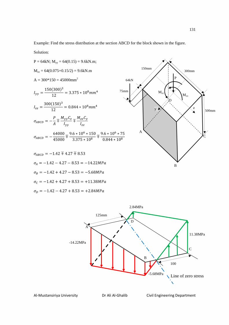
131
Al-Mustansiriya University Dr Ali Al-Ghalib Civil Engineering Department
Example: Find the stress distribution at the section ABCD for the block shown in the figure.
Solution:
P = 64kN; Myy = 64(0.15) = 9.6kN.m;
Mzz = 64(0.075+0.15/2) = 9.6kN.m
A = 300*150 = 45000mm2
Ð � 150(300)H12 = 3.375 ∗ 10JJ
Ð�� = 300(150)H12 = 0.844 ∗ 10JJ
��)?x = − � ∓ ( ��Ð ∓ (��� Ð��
��)?x = − 6400045000 ∓ 9.6 ∗ 10= ∗ 1503.375 ∗ 10 ∓ 9.6 ∗ 10= ∗ 750.844 ∗ 10
��)?x = −1.42 ∓ 4.27 ∓ 8.53
�� = −1.42 − 4.27 − 8.53 = −14.22(�<
�) = −1.42 + 4.27 − 8.53 = −5.68(�<
�? = −1.42 + 4.27 + 8.53 = +11.38(�<
�x = −1.42 − 4.27 + 8.53 = +2.84(�<
Myy Mzz
P
z y
150mm 300mm
A
B
C
D
500mm
64kN
75mm
A
B
C
D
-14.22MPa
-5.68MPa
11.38MPa
2.84MPa
Line of zero stress
125mm
100

132
Al-Mustansiriya University Dr Ali Al-Ghalib Civil Engineering Department
Example: A short 100mm square steel bar with a 50mm diameter axial hole is built at the base and is loaded at the top as shown in the figure. Determine the value of the force P so that the maximum normal stress at the fixed-end would not exceed 140MPa.
Solution:
� 6100)� − R(50)�4 = 8037JJ�
Ð = 100(100)H12 − R(25)
4 = 8.03 ∗ 10=JJ
�� = − �d]a30 − (�ab\30 ∗ 400) ∗ �Ð + (�d]a30 ∗ 50) ∗ �Ð = 140(�<
140 = − �d]a308037 − (�ab\30 ∗ 400) ∗ 508.03 ∗ 10= + (�d]a30 ∗ 50) ∗ 508.03 ∗ 10=
140 = −1.078 ∗ 10L � − 1.25 ∗ 10LH� + 2.7 ∗ 10L � = −1.088 ∗ 10LH�
140 = �954.4 => � = 129NI
�) = − �d]a30 + (�ab\30 ∗ 400) ∗ �Ð − (�d]a30 ∗ 50) ∗ �Ð = 140(�<
140 = − �d]a308037 + (�ab\30 ∗ 400) ∗ 508.03 ∗ 10= − (�d]a30 ∗ 50) ∗ 508.03 ∗ 10=
140 = −1.078 ∗ 10L � + 1.25 ∗ 10LH� − 2.7 ∗ 10L � = +8.72 ∗ 10L �

133
Al-Mustansiriya University Dr Ali Al-Ghalib Civil Engineering Department
140 = P�� | => � = 161NI. The safe force P=129kN
Example: A cast iron block is loaded as shown in the figure. Determine the stresses acting normal to a section (ABCD) at 0.5m from the top, and locate the line of zero stress. Solution: Myy = 10kN * 0.5m = 5.0kN.m Mzz = 15kN * 0.38m = 5.7kN.m
Ð = 100(200)H12 = 6.67 ∗ 10|JJ
Ð�� = 200(100)H12 = 1.67 ∗ 10|JJ
��)?x = − � ∓ ( ��Ð ∓ (��� Ð��
��)?x = ∓ 5.0 ∗ 10= ∗ 1006.67 ∗ 10| ∓ 5.7 ∗ 10= ∗ 501.67 ∗ 10|
��)?x = ∓7.5 ∓ 17.1 �� = +7.5 + 17.1 = +24.6(�<
�) = −7.5 + 17.1 = +9.6(�<
�? = −7.5 − 17.1 = −24.6(�<
�x = +7.5 − 17.1 = −9.6(�<
Myy
Mzz
z y
50mm
100mm
A
B
C
D
500mm
100mm
50mm 10kN
120
15kN
A
B
C
D
+24.6MPa
+9.6MPa
-24.6MPa
-9.6MPa
Line of zero stress
71.9mm

134
Al-Mustansiriya University Dr Ali Al-Ghalib Civil Engineering Department
Example: A small dam of triangular shape as shown in the figure is made from concrete, which weighs 2550kg/m3. Find the normal stress distribution at the base AB when the water behind the dam is as indicated in the figure. For the purpose of calculation, consider one lineal meter of the dam in the direction perpendicular to the plane of paper.
é � � � ¡12 (3.3J) Õ10NIJH Ö¢ (3.3J)(1J) = 54.45NI
� = � = ¡12 (2.1J)(3.6J)(1J)¢ Õ25NIJH Ö = 94.5NI
( = é(1.1J) − �(0.35J) = 54.45NI ∗ 1.1J − 94.5NI ∗ 0.35J = 26.82NIJ
�) = − � + (�Ð = − 94.5(2.1)(1) + 26.82(1.05)�(�.�)4
��= −45 + 36.5 = − 8.5NIJ� (d]J�e`aab]\)
�� = − � − (�Ð = − 94.5(2.1)(1) − 26.82(1.05)�(�.�)4
��= −45 − 36.5 = − 81.5NIJ� 6d]J�e`aab]\7

135
Al-Mustansiriya University Dr Ali Al-Ghalib Civil Engineering Department
2. Superposition of shearing stresses
Example: Find the maximum shearing stress due to the applied forces in the plane AB of the 10mm diameter circular shaft.
Solution:
a. Shear stress due to the shear force
τ @ A and B =0;
τ @ C, D and E = τmax .
� �ÛÐ�
8B� � �23∗¡$��#�# ∗�%∗�)4$ �¢$(�)%
% ∗�3 = 4.24(�<
b. Shear stress due to the torque
τ @ C =0;
τ @ A, B, D and E = τmax .
8B� = �@¨
8B� � 20000 ∗ 5�� (5 ) = 101.86(�<
8B�]dd[ea@�]b\Tl � 4.24 + 101.86 = 106.1(�<
A
E DC
B
t max
A
E DC
B
T

136
Al-Mustansiriya University Dr Ali Al-Ghalib Civil Engineering Department
Example: Find the maximum shearing stress due to the applied forces in the fixed end
50kN1
00
mm
50250mm
100kN
Torque (T) = 50* 0.05/2 = 1.25kN.m
Shear force (V) = 50kN
Bending moment (M) = 50*0.25 = 12.5kN.m
Axial force (P) = 100kN
• Normal stresses
Axial stress:
�B�DB� � P� � �3333323∗�33 = 20(�<
Bending stresses:
��AE&DEF = (�Ð = 12.5 ∗ 10= ∗ 5023∗�334��
= 150(�<
Using the superposition principal:
���� = + � + (�Р= 20 + 150 = 170(�<
���� = + � − (�Ð = 20 − 150 = −130(�<
• Shear stresses a) Due to the shear force
τ @ A, B, E and F =0;
τ @ C, O and D is τmax .

137
Al-Mustansiriya University Dr Ali Al-Ghalib Civil Engineering Department
� �ÛÐ�
8B� � 50 ∗ 10H ∗ [50 ∗ 50 ∗ 25]23(�33)4
�� ∗ 50 = 15(�<
b) Due to the torque
τ @ A, B, E, F and O =0;
τ @ C, and D is τmax
8B� = ��<�� a /b = 100/50 = 2 (α = 0.246)
8B� � 1.25 ∗ 10=0.246 ∗ 100 ∗ (50)� = 20.33(�<
8B�)��8��«E&@ë � ![`T]� � ![`T]� � 15 + 20.33 = 35.33(�<

138
Al-Mustansiriya University Dr Ali Al-Ghalib Civil Engineering Department
Homework
1. An inclined beam having a cross-section of 0.2m by 0.3m supports a downward load as shown in the figure. Determine the maximum stress acting normal to the section A-A. Neglect the weight of the member.
0.3m
2. An Aluminum –alloy block is loaded as shown in the figure. The application of this load produces a tensile strain of 500 x 10-6 at gage A. Calculate the magnitude of the applied load P. Let E = 100GPa.
P
z y
120mm 180mm
400mm
20mm
Gage A

139
Al-Mustansiriya University Dr Ali Al-Ghalib Civil Engineering Department
Chapter Eight: Analysis of Plane Stress and Strain
In fact, if a plane element is taken out from a body, it will be subjected to the normal stresses σx
and σy together with the shearing stress τxy, as shown in the figure below. No stresses are assumed to act on the element in the z-direction.
We shall assume that the stresses σx, σy and τxy are known. Regularly, it is desirable to investigate
the state of stress on a plane perpendicular to the axis x’ of an angle θ, measured counter-clockwise to the x-axis, as shown in the figure. Assume the area of the inclined plane is one unit. Then, by applying the equations of static equilibrium to the forces on the wedge, stresses σx and
τxy can be found:
From ∑��ì � 0
��í (1) = ��(cos §)( cos §) + � (ab\§)(d]a§) + � (sin §)( sin §) + � (cos §)( sin §)
��í = ��(cos� §) + � (sin� §) + 2� (sin §) (cos §)
��í = ��(1 + d]a2§2 ) + � (1 − d]a2§2 ) + � (ab\2 §)
��í = (�� + � 2 ) + �� − � 2 (d]a2§) + � (ab\2 §) ⋯⋯61)
Similarly, from ∑ � ì = 0

140
Al-Mustansiriya University Dr Ali Al-Ghalib Civil Engineering Department
�í í61) = � (cos §)( cos §) − ��(ab\§)(d]a§) − � (sin §)( sin §) + � (cos §)(ab\§)
�í í = � (cos� § − sin� §) − ��(ab\§)(d]a§) + � (cos §)(ab\§)
�í í = − ��� − � 2 � ab\2§ + � d]a2§ ⋯ ⋯ (2)
Equations 1 and 2 are the general expressions for the normal and shearing stresses, respectively,
on any plane located by the angle θ and caused by a known system of stresses.
Sign convention
σx, σy= + tensile
σx, σy= - compressive
τxy = + on the right-hand face, tends to rotate the element counterclockwise
θ = + counterclockwise
Principal Stresses
To find the direction of the maximum or minimum normal stress, Equation 1 is differentiated with respect to θ, and the derivative is set equal to zero i.e.
&opí&ò = − opLoó� ∗ 2ab\2§ + 2� (cos2 §) = 0
Therefore, tan 2§� = öpó(opLoó)/� ⋯ ⋯ (3)
The two planes defined by the angles θ1 are called principal planes. The normal stresses that exist on these planes are designated as principal stresses. They are the maximum and minimum values of the normal stress in the element under consideration. The expression for the maximum normal stress, denoted by σ1, and the minimum normal stress, denoted by σ2, become:

141
Al-Mustansiriya University Dr Ali Al-Ghalib Civil Engineering Department
��,� = �� + � 2 ∓ ÷��� − � 2 �� + (� )� ⋯⋯ 64)
Maximum shearing stresses
To determine the maximum value of the shearing stress, Equation 2 should be differentiated with respect to the angle θ2 and set this derivative equal to zero. Therefore:
!�′ ′!§ = −��� − � �d]a2§ − 2� ab\2§ = 0
tan 2§� = − opLoó� � ⋯⋯65)
The values of sin2θ2 and cos2θ2 may now be substituted in Equation 2 to yield the maximum and minimum values of the normal stresses.
Therefore, the maximum shearing stress can be found from the Equation 6:
8B�,8DE = ∓÷��� − � 2 �� + (� )� ⋯⋯66)
Mohr’s Circle of Stress
��í = (�� + � 2 ) + �� − � 2 (d]a2§) + � (ab\2 §) ⋯ ⋯ (1)
�ì í = − ��� − � 2 � ab\2§ + � cos2θ ⋯ (2)
Equation 1)2 + Equation 2)2, will lead to eliminate the variable θ as in the following expression:
(��í − (�� + � 2 ))� + (�ì í)� = (�� − � 2 )� + (� )� ⋯ ⋯ (7)
Compare Equation 7 with the following standard equation:
(n − <)� + (g)� = e�
Therefore, Equation 7 represents a circle equation whereby its centre (a, 0) is:
< = �� + � 2
And its radius (r) is:

142
Al-Mustansiriya University Dr Ali Al-Ghalib Civil Engineering Department
e � � � ù6�� U � 2 )� + (� )�

143
Al-Mustansiriya University Dr Ali Al-Ghalib Civil Engineering Department
The constructed circle is named a circle of stress or Mohr’s circle of stress. It is so named in honor of the German Professor in civil engineering Otto Christian Mohr (1835-1918), who in 1895 suggested its use in the stress analysis.
Important conclusions on Mohr’s circle of stress
1. The largest possible normal stress is σ1; the smallest possible normal stress is σ2. No shearing stresses exist together with either one of these principal stresses.
2. The largest shearing stress τmax is numerically equal to the radius of the circle, also to (σ1-σ2)/2. A normal stress equal to (σ1 + σ2)/2 acts on each plane of the maximum shearing stress.
3. If σ1 = σ2, Mohr’s circle degenerates into a point, and no shearing stresses at all develop in the xy plane.
4. If σx + σy = 0, the centre of Mohr’s circle coincides with the origin of σ-τ coordinates, and the state of pure shear stress exists.
5. The sum of the normal stresses on any two mutually perpendicular planes is invariant, i.e.
σx+ σy = σ1 + σ2 = σx’ + σy’ = constant
Construction of Mohr’s circle of stress
1. Make a sketch of the element for which the normal stresses and shearing stresses are
known with the proper sense.
2. Set up a rectangular coordinate system of axes. The horizontal x-axis is the normal stress axis and the vertical y-axis is the shearing stress axis.
3. Locate the centre of the circle, which is on the horizontal axis at a distance of (σx+ σy)/2 from the origin.
Otto MohrOtto MohrOtto MohrOtto Mohr
The famous German civil engineer Otto Christian Mohr (1835–1918) was both a theoretician and a practical designer. He was a professor at the Stuttgart Polytechnic and later at the Dresden Polytechnic. He developed the circle of stress in1895.
Mohr made numerous contributions to the theory of structures, including the Williot-Mohr diagram for truss displacements, the moment-area method for beam deflections, and the Maxwell-Mohr method for analyzing statically indeterminate structures.

144
Al-Mustansiriya University Dr Ali Al-Ghalib Civil Engineering Department
4. Compute the radius of the circle of value e � ù6opLoó� 7� � 6� 7� and draw the circle.
5. The points of the circle intersection with horizontal x-axis represent the largest normal stresses (principal stresses) of coordinates (σ1, 0) and (σ2, 0).
6. Draw a line between the centre of the circle and a point called the control point A. The coordinates of the control point is A (σx , τxy). Alternatively, the control point could be B (σy , -τxy).
7. To determine the direction and the sense of the stresses, each angle on the Mohr’s circle represents twice the angle on the direction of the stress on the real element.
8. The clockwise rotation on the circle represents counter-clockwise rotation on the element and vice versa.
Example 1: Draw Mohr’s circle of stress for the state of plane stress shown on the element below.
a) Show the planes on which the principal stresses act, and for each plane indicate its direction and sense.
b) Same as (a) for the maximum shearing stresses. c) Find the magnitude and the sense of the normal and shearing stresses on an inclined plane
of 30° from the vertical plane.
Solution:
The centre of the circle is C (a, 0) where:
< � �� � � 2 = −2 + 42 = 1
Therefore, C (1, 0)
And its radius (r) is:
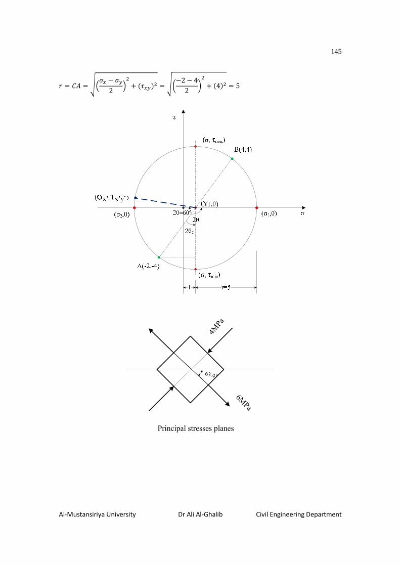
145
Al-Mustansiriya University Dr Ali Al-Ghalib Civil Engineering Department
e � � � ÷��� U � 2 �� + (� )� = ÷Õ−2 − 42 Ö� + (4)� = 5
4MPa
6MPa
63.4°
Principal stresses planes
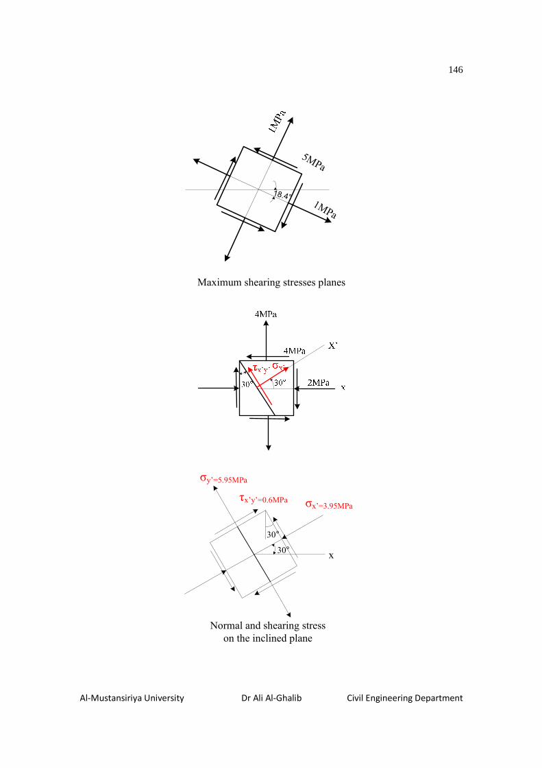
146
Al-Mustansiriya University Dr Ali Al-Ghalib Civil Engineering Department
1MPa
5MPa
18.4°
Maximum shearing stresses planes
σx’=3.95MPa
30°
τx’y’=0.6MPa
σy’=5.95MPa
x
30°
Normal and shearing stress
on the inclined plane

147
Al-Mustansiriya University Dr Ali Al-Ghalib Civil Engineering Department
Example 2: For the state of stress shown on the element below, use Mohr’s circle of stress to determine:
a) The principal stresses and the direction of their planes. b) The maximum shearing stresses and the direction of their planes.
Solution: σx= +20; σy= +40; τxy= +40
The centre of the circle is C (a, 0) where:
< � �� � � 2 = +20 + 402 = 30
Therefore, C (30, 0)
And its radius (r) is:
e = � = ÷��� − � 2 �� + (� )� = ÷Õ+20 − 402 Ö� + (40)� = 41.2
The Principal Stresses are:
��,� = �� + � 2 ∓ ÷��� − � 2 �� + (� )� = 20 + 402 ∓ ÷Õ20 − 402 Ö� + (40)�
��,� = 30 ∓ 41.2 = L��.�ÒPB|�.�ÒPB
The maximum shearing stresses are:
8B�8DE = ÷��� − � 2 �� + (� )� = ÷Õ+20 − 402 Ö� + (40)� = ∓41.2(�<

148
Al-Mustansiriya University Dr Ali Al-Ghalib Civil Engineering Department
The direction of maximum normal stresses on the Mohr’s circle is:
2§� = 14° + 90° = 104°��
The direction of maximum shearing stresses on the Mohr’s circle is:
sin2§� = 1041.2 => 2§� = 14° ��

149
Al-Mustansiriya University Dr Ali Al-Ghalib Civil Engineering Department
30MPa
30MPa
41.2MPa
7°
Maximum shearing stresses planes
Example 3: Draw Mohr’s circle of stress for the states of stress given in the figure.
a) Clearly show the planes on which the principal stresses act, and for each stress indicate with arrows its direction and sense.
b) Same as (a) for the maximum shearing stresses and the associated normal stresses.
Solution: σx= +10; σy= +10; τxy= 0
The centre of the circle is C (a, 0) where:
< � �� � � 2 = +10 + 102 = 10
Therefore, C (10, 0)
And its radius (r) is:

150
Al-Mustansiriya University Dr Ali Al-Ghalib Civil Engineering Department
e � ÷��� U � 2 �� + (� )� = ÷Õ+10 − 102 Ö� + (0)� = 0

151
Al-Mustansiriya University Dr Ali Al-Ghalib Civil Engineering Department
Homework
1. A plane element is subject to the stresses shown in the figure below. Using Mohr’s circle, determine (a) the principal stresses and their directions, and (b) the maximum shearing stresses and the directions of the planes on which they occur. Ans: σ1 = 20MPa at 63.4°, σ2 = -80MPa, τmax = 50MPa at 18.4°
2. A plane element removed from a thin-walled circular tube loaded in torsion is subject to the shearing stresses shown in the figure below. Determine the principal stresses existing in this element and the directions of the planes on which they occur. Ans: 50MPa at 45°
3. Draw each one of the infinitesimal elements A, B and C individually, and indicate the stress state on the isolated element. For each stress, show the direction and sense by arrows.

152
Al-Mustansiriya University Dr Ali Al-Ghalib Civil Engineering Department
Transformation Equations of Plane Strain
It follows that an element in plane strain has no normal strain εz in the z-direction and no shear
strains γxz and γyz in the xz and yz planes, respectively. Thus, plane strain is defined by the following conditions:
εz = 0; γxz = 0; γyz = 0
The transformation equations for plane stress can also be used for the stresses in plane strain.
Only, the symbol σ must be replaced by ε and τ must be replaced by γ/2. Therefore, the transformation expressions of plane strain become:
i�í � 6i� � i 2 ) + i� − i 2 (d]a2§) + �� 2 (sin2 §) ⋯ ⋯ (8) ��ì í2 = − �i� − i 2 � ab\2§ + �� 2 cos2θ
��ì í = −�i� − i �ab\2§ + �� cos2θ ⋯ ⋯ (9)
Sign convention
εx, εy= +elongation
εx, εy= - contraction
γxy = + elongation for the diagonal of positive slope
θ = + counterclockwise
Principal strains
i�,� = i� + i 2 ∓ ÷�i� − i 2 �� + (�� 2 )� ⋯⋯610)
γxy = 0, No shear strain associated with the principal strains

153
Al-Mustansiriya University Dr Ali Al-Ghalib Civil Engineering Department
Principal strains exist on perpendicular planes with the principal angles θ1 calculated from the following equation:
tan2§� = �� (i� − i ) ⋯ ⋯ (11)
Maximum shear strain
�8B�2 = ∓÷�i� − i 2 �� + (�� 2 )� ⋯⋯ 612) In the directions of maximum shear strain, the normal strains are:
i � i� � i 2 ⋯ ⋯ (13)
The maximum shear strains in the xy plane are associated with axes at 45° to the directions of the principal strains.
Mohr’s Circle of Plane Strain
Mohr’s circle for plane strain is constructed in the same manner as the circle for plane stress, as
illustrated in the figure below. Normal strain ε is plotted as the abscissa (positive to the right)
and one-half the shear strain (γxy/2) is plotted as the ordinate (positive upward). The center C of
the circle has an abscissa equal to a( εaverage) (Eq. 13).
2
2
)2
()2
(γεε xyyxr +=
−

154
Al-Mustansiriya University Dr Ali Al-Ghalib Civil Engineering Department
Example: An infinitesimal element on a body contracts along the x-axis by 0.0005m/m, elongates along the y-axis by 0.0003m/m and the shear stain of this element is -0.0006rad, as shown below. Determine the principal strains and their directions.
Solution:
εx= -5 x 10⁻⁴
εy= +3 x 10⁻⁴
γxy = -6 x 10⁻⁴ (contraction for the diagonal of positive slope)
� Õi� � i 2 , 0Ö => � ûU5x10L + 3x10L 2 , 0ý => �(−1,0)x10L
e = ÷û−5x10L − 3x10L 2 ý� + (−6x10L
2 )� � 5x10L
ε1= +4 x 10⁻⁴
ε2= -6 x 10⁻⁴
2θ1 = 143.13° counterclockwise
4x10⁻⁴
71.56
Principal strains
6x10⁻⁴

155
Al-Mustansiriya University Dr Ali Al-Ghalib Civil Engineering Department
Chapter Eleven: Deflection of Beams
Under the action of lateral applied forces, the axis of a beam deflects from its initial position. Deflection amounts in the structural elements must be very small in order to:
• Avoid the undesirable psychological feelings on the occupants.
• Minimize or prevent the failure in finishing materials.
Figure 1: Deflection of a cantilever beam
Therefore, specifications limit the maximum permissible deflection to a certain value, span/360, span/ 480…etc.
In this chapter, only deflections caused by bending moments are considered. Additionally, the elastic deflections of the beams are only considered.
Double Integration Method
In chapter five, the relationship between the curvature and the bending moment is derived, and given as:
Ï � 1¦ = (lÐ ⋯⋯ 61)
Figure 2: Behavior of a beam in bending

156
Al-Mustansiriya University Dr Ali Al-Ghalib Civil Engineering Department
In analytical geometry, the curvature of a line is defined as:
1¦ = &# &�#
¡1 + �& &���¢4#⋯ ⋯ (2)
In small deflections theory, the square of the slope, (dy/dx)2, is a negligible quantity because the deflection of the elastic curve is very small.
Therefore, the curvature of a line becomes:
1¦ ≈ !�g!n� ⋯ ⋯ (3)
!�g!n� ≈ (lÐ ⋯⋯64)
Alternatively, Equation 4 can be written as:
lÐ !�g!n� ≈ (6n7⋯⋯65) Examples
Determine the general formula for estimating the rotation and deflection at any section of the beams shown below. Also, find the maximum rotation and maximum deflection. Assume EI= constant.
1. lÐ &# &�# � (6n7 lÐ !�g!n� � UJ
Integrate both sides of the above equation:
lР& &� � UJn � ��
Apply the Boundary Conditions (B.C):
@n � 0; !g!n � 0 => �� = 0
lÐ !g!n � UJn⋯@]T<Tb]\`_[<Tb]\
L
Elastic curve
mm
B.M.D-
m
x

157
Al-Mustansiriya University Dr Ali Al-Ghalib Civil Engineering Department
@n � j;Õ!g!nÖ8B� � §8B� � UJjlÐ
Integrate both sides of the rotation equation:
lÐg � UJn�2 � �� Apply the Boundary Conditions (B.C):
@n � 0; g � 0 => �� = 0
lÐg � UJn�2 ⋯ ë`fc`dTb]\`_[<Tb]\ @n � j;g8B� � ∆8B�� UJj�2lÐ
2. lÐ &# &�# � (6n7 lÐ !�g!n� � U�j � �n
Integrate both sides of the above equation:
lР& &� � U�jn � P�#� � �� Apply the Boundary Conditions (B.C):
@n � 0; !g!n � 0 => �� = 0
lÐ !g!n � U�jn � �n�2 ⋯@]T<Tb]\`_[<Tb]\
@n � j;Õ!g!nÖ8B� � §8B� � U �j�2lÐ Integrate both sides of the rotation equation:
lÐg � U�jn�2 + �nH6 + ��
Apply the Boundary Conditions (B.C):
@n � 0; g � 0 => �� = 0
Elastic curve
x
L
P
B.M.D-
PL
P
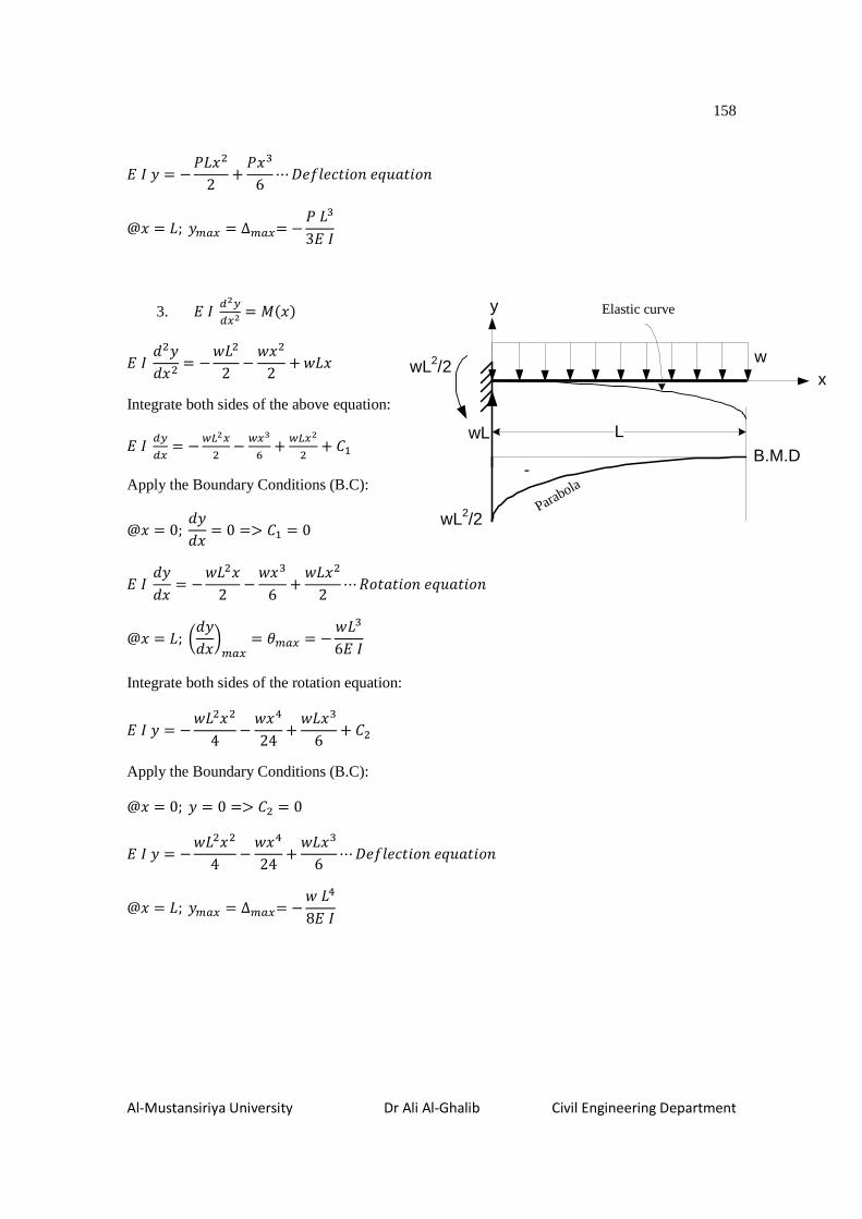
158
Al-Mustansiriya University Dr Ali Al-Ghalib Civil Engineering Department
lÐg � U�jn�2 + �nH6 ⋯ ë`fc`dTb]\`_[<Tb]\
@n � j;g8B� � ∆8B�� U�jH3lÐ
3. lÐ &# &�# � (6n7 lÐ !�g!n� � U^j�2 − ^n�
2 + ^jn
Integrate both sides of the above equation:
lР& &� � UXk#�� U X�4= � Xk�#� � ��
Apply the Boundary Conditions (B.C):
@n � 0; !g!n � 0 => �� = 0
lÐ !g!n � U^j�n2 − ^nH6 + ^jn�
2 ⋯ @]T<Tb]\`_[<Tb]\
@n � j;Õ!g!nÖ8B� � §8B� � U ^jH6lÐ Integrate both sides of the rotation equation:
lÐg � U^j�n�4 − ^n 24 + ^jnH
6 + ��
Apply the Boundary Conditions (B.C):
@n = 0; g � 0 => �� = 0
lÐg � U^j�n�4 − ^n 24 + ^jnH
6 ⋯ ë`fc`dTb]\`_[<Tb]\ @n � j;g8B� � ∆8B�� U^j 8lÐ
Elastic curve
x
L
w
B.M.D-
y
wL
wL2/2
wL2/2Para
bola

159
Al-Mustansiriya University Dr Ali Al-Ghalib Civil Engineering Department
4. lÐ &# &�# � (6n7 lÐ !�g!n� � U^nH6j
Integrate both sides of the above equation:
lР& &� � UX�%� k � ��
Apply the Boundary Conditions (B.C):
@n � j;!g!n � 0 => �� = ^jH24
lÐ !g!n � U^n 24j + ^jH24 ⋯ @]T<Tb]\`_[<Tb]\
@n � 0; Õ!g!nÖ8B� � §8B� � � ^jH24lÐ Integrate both sides of the rotation equation:
lÐg � U ^n2120j − ^jHn24 + ��
Apply the Boundary Conditions (B.C):
@n = j; g � 0 => �� = − ^j 30
lÐg � U ^n2120j − ^jHn24 − ^j 30 ⋯ ë`fc`dTb]\`_[<Tb]\
@n � 0; g8B� � ∆8B�� U ^j 30lÐ
w
L
y
x
wL/2
wL2/6

160
Al-Mustansiriya University Dr Ali Al-Ghalib Civil Engineering Department
5. lР&# &�# � (6n7 ; lР&# &�# � Xk�� U X�#�
Integrate both sides of the above equation:
lР& &� � Xk�# U X�4= � ��
Apply the Boundary Conditions (B.C):
@n � j2 ; !g!n � 0 => �� = − ^jH24
lÐ !g!n � ^jn�4 − ^nH6 − ^jH
24 ⋯ @]T<Tb]\`_[<Tb]\
@n � 0]en � j;Õ!g!nÖ8B� � §8B� � U ^jH24lÐ Integrate both sides of the rotation equation:
lÐg � ^jnH12 − ^n 24 − ^jHn24 + ��
Apply the Boundary Conditions (B.C):
@n = 0; g � 0 => �� = 0
lÐg � ^jnH12 − ^n 24 − ^jHn24 ⋯ ë`fc`dTb]\`_[<Tb]\
@n � k� ; g8B� � ∆8B�� U 2Xk%H qÓ Very popular value of maximum deflection in a simply
supported beam

161
Al-Mustansiriya University Dr Ali Al-Ghalib Civil Engineering Department
6. Part AB: 0 ≤ n ≤ 2<; lÐ &# &�# � (6n7; lÐ !2g!n2 = �n3
2a a
A CB
P
xxP/3 2P/3
Integrate both sides of the above equation:
lÐ & &� � P�#= � ��⋯⋯61)
Integrate both sides of the rotation equation:
lÐg � �n318 + ��n + �� ⋯ ⋯ (2)
Part BC: 2< ≤ n ≤ 3<; lÐ !2g!n2 = �n3 − �(n − 2<) = 2�3 (3< − n)
lÐ !g!n � 2�3 û3<n − n�2 ý + �H ⋯ ⋯ (3)
lÐg � 2�3 û3<n�2 − nH
6 ý + �Hn + � ⋯ ⋯ (4)
The four constants are found by using two boundary conditions known as:
@n = 0; g � 0<\!@n � j; g � 0
Also, two continuity conditions must be applied at point B:
@�]b\TÑ6n � 2<); !g!n |�) � !g!n |)?
@�]b\TÑ6n � 2<); g|�) � g|)?
From Equation 2: 0 = �(0)3
18 + ��(0) + �� => �� � 0 ⋯ (5)
From Equation 4:

162
Al-Mustansiriya University Dr Ali Al-Ghalib Civil Engineering Department
0 = 2�3 û3<(j)�2 − (j)H
6 ý + �H(j) + � ⋯ (6)
From Equation 1 and Equation 3:
�(2<)�6 + �� = 2�3 û3<(2<) − (2<)�
2 ý + �H ⋯ (7)
From Equation 2 and Equation 4:
�(2<)H18 + �1(2<) + �2 = 2�3 û3<(2<)�
2 − (2<)H6 ý + �H(2<) + � ⋯ (8)
Solving Equations (5-8) simultaneously, we get:
�� = − 4�<�9
�� = 0
�H = − 22�<�9
� = 4�<H3
Equations (1-4) become:
Part AB: 0 ≤ n ≤ 2<
lÐ !g!n � �n�6 − 4�<�9 ⋯ (9)
lÐg � �n318 − 4�n<29 ⋯ (10)
Part BC: 2< ≤ n ≤ 3<
lÐ !g!n � 2�3 û3<n − n�2 ý − 22�<�
9 ⋯ (11)
lÐg � 2�3 û3<n�2 − nH
6 ý − 22�n<�9 + 4�<H
3 ⋯ (12)
By inspecting the elastic curve, the maximum deflection occurs at point D, somewhere in the region AB. At point D the slope must be zero.

163
Al-Mustansiriya University Dr Ali Al-Ghalib Civil Engineering Department
Therefore, from Equation 9:
0 = �n�6 − 4�<�
9
x= 1.633a
Substituting in Equation 10:
lÐg8B� � �61.633<)318 − 4�(1.633<)<2
9
g8B� � U0.484 �(<)3lÐ
Macaulay’s Method (Singularity Functions)
The techniques discussed in the preceding section are adequate if the loadings are continuously
varying over the length of the beam. Nevertheless, if concentrated forces or moments are present,
a distinct pair of shearing force and bending moment equations must be written for each interval
between such concentrated forces or moments. Although this presents no fundamental
difficulties, it is usually elaborated approach and gives very cumbersome results. These results
are particularly unwieldy to work with in dealing with deflections of beams.
As a minimum, some shortness of representation can be achieved by introduction of singularity or
half-range functions. Let us introduce, by definition, the pointed brackets <x- a> and define this
quantity to be zero if (x – a) < 0, that is, x < a, and to be simply (x – a) if (x – a) > 0, that is, x > a.
That is, a half-range function is defined to have a value only when the argument is positive. When
the argument is positive, the pointed brackets behave just as ordinary parentheses.
Solution of example 6 by using singularity functions:
lÐ &# &�# � (6n7; (6n7 � � < n W1
3 − � < n − 2< >1

164
Al-Mustansiriya University Dr Ali Al-Ghalib Civil Engineering Department
lÐ !2g!n2 = � < n >�3 − � < n − 2< >�
Integrate both sides of the above equation:
lÐ !g!n = � < n >�6 − � < n − 2< >�
2 + �� ⋯ ⋯ (13)
Integrate both sides of the rotation equation:
lÐg = � < n >H18 − � < n − 2< >H
6 + ��n + ��
Apply the two boundary conditions known as:
@n = 0; g � 0<\!@n � 3<; g � 0
�� = 0
0 = �(3<)H18 − �(3< − 2<)H
6 + ��(3<)
�� = − 4�<�9
Therefore, the deflection equation of the whole beam can be written as:
lÐg = � < n >H18 − � < n − 2< >H
6 − 4�<�n9 ⋯ ⋯ (14)
Once again, by inspecting the elastic curve, the maximum deflection occurs at point D, somewhere in the region AB. At point D the slope must be zero.
Therefore, from Equation 13:
0 = �n�6 − 4�<�
9
x= 1.633a
Substituting in Equation 14:
lÐg8B� � �61.633<)318 − 4�(1.633<)<2
9
g8B� � U0.484 �(<)3lÐ

165
Al-Mustansiriya University Dr Ali Al-Ghalib Civil Engineering Department
7. Using the singularity functions, determine the deflection equation of the cantilever beam loaded as shown below.
lÐ &# &�# � (6n7; (6n7 � U� < n W1− 2� < n − j4 >1
Therefore, the differential curvature equation for the beam becomes:
lÐ !2g!n2 = −� < n >�− 2� < n − j4 >�
Integrate both sides of the above equation:
lÐ !g!n = −� < n >�2 − � < n − j4 >�+ ��
The second integration leads to:
lÐg = −� < n >H6 − � < n − k >H
3 + ��n + ��
Apply the first boundary condition known as:
@n = j; !g!n � 0 0 = − �j�
2 − �(3j4 )� + ��
�� = �j�2 + 9�j�
16
�� = 17�j�16
Apply the second boundary condition known as:
@n = j; g � 0:
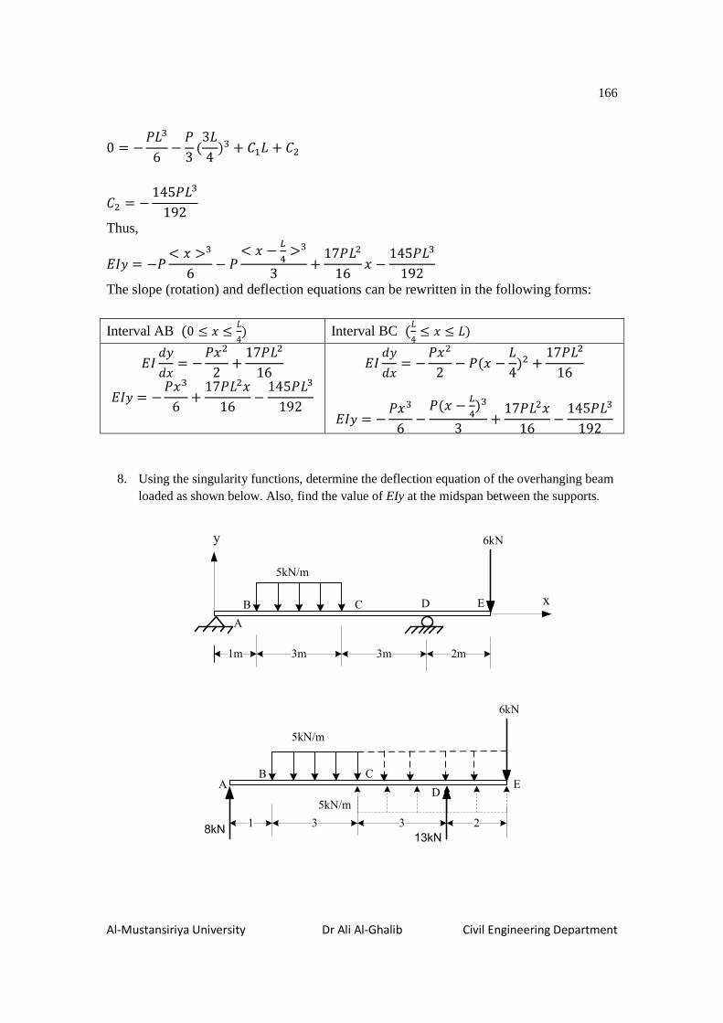
166
Al-Mustansiriya University Dr Ali Al-Ghalib Civil Engineering Department
0 = − �jH6 − �3 (3j4 )H + ��j + ��
�� = − 145�jH192
Thus,
lÐg = −� < n >H6 − � < n − k >H
3 + 17�j�16 n − 145�jH
192
The slope (rotation) and deflection equations can be rewritten in the following forms:
Interval AB (0 ≤ n ≤ j4) Interval BC (j4 ≤ n ≤ j) lÐ !g!n = − �n�
2 + 17�j�16
lÐg = − �nH6 + 17�j�n16 − 145�jH
192
lÐ !g!n = − �n�2 − �(n − j4)� + 17�j�
16
lÐg = − �nH6 − �(n − k )H
3 + 17�j�n16 − 145�jH192
8. Using the singularity functions, determine the deflection equation of the overhanging beam loaded as shown below. Also, find the value of EIy at the midspan between the supports.
x
1m
A
B
y 6kN
3m 3m
5kN/m
C D E
2m
8kN1
AB
6kN
3 3
5kN/m
C
DE
2
13kN
5kN/m

167
Al-Mustansiriya University Dr Ali Al-Ghalib Civil Engineering Department
(6n7 � 8n U 5 < n − 1 >�2 + 5 < n − 4 >�
2 + 13 < n − 7 >
Therefore, the differential curvature equation for the elastic curve becomes:
lÐ !2g!n2 = 8n U 5 < n − 1 >�2 + 5 < n − 4 >�
2 + 13 < n − 7 >
Integrate both sides of the above equation twice gives:
lÐ !g!n = 4n� U 5 < n − 1 >H6 + 5 < n − 4 >H
6 + 13 < n − 7 >�2 + ��
lÐg = 4nH3 − 5 < n − 1 > 24 + 5 < n − 4 >
24 + 13 < n − 7 >H6 + ��n + ��
To find the value of C2, we apply the B.C. @x=0; y=o. That gives C2=0.
Also, to obtain C1, we note that @x=7; y=0. This gives:
0 = 467)H3 − 5(6)
24 + 5(3) 24 + 0 + ��(7) + 0
C1= -29.17
lÐg = 4nH3 − 5 < n − 1 > 24 + 5 < n − 4 >
24 + 13 < n − 7 >H6 − 29.17n
In order to obtain the midspan deflection, the value x=3.5m is substituted in the
deflection equation and ignoring the negative values of the pointed brackets <x-4>4 and
<x-7>3. We find:
lÐg = 463.5)H3 − 5 < 3.5 − 1 >
24 − 29.17(3.5)
g = − 53lÐ NI − JH

168
Al-Mustansiriya University Dr Ali Al-Ghalib Civil Engineering Department
Note: example on writing the moment expression for the entire beam when a couple
applied at a point:
(6n7 � (3j n U (3 < n U < W3
Example: a simply supported beam carries a triangularly distributed load.
Because of the symmetry of the beam and loading, only the moment equation for the part
AB is used.
lÐ !�g!n� � 24n − nH2
lÐ !g!n � 12n� − n 8 + ��
lÐg � 4nH − n240 + ��n + ��
In order to work out the constant of integration, it is obvious that at support A (x=0; y=0). In
addition and because of symmetry, at point B (midspan of the beam) x=4; dy/dx=0.
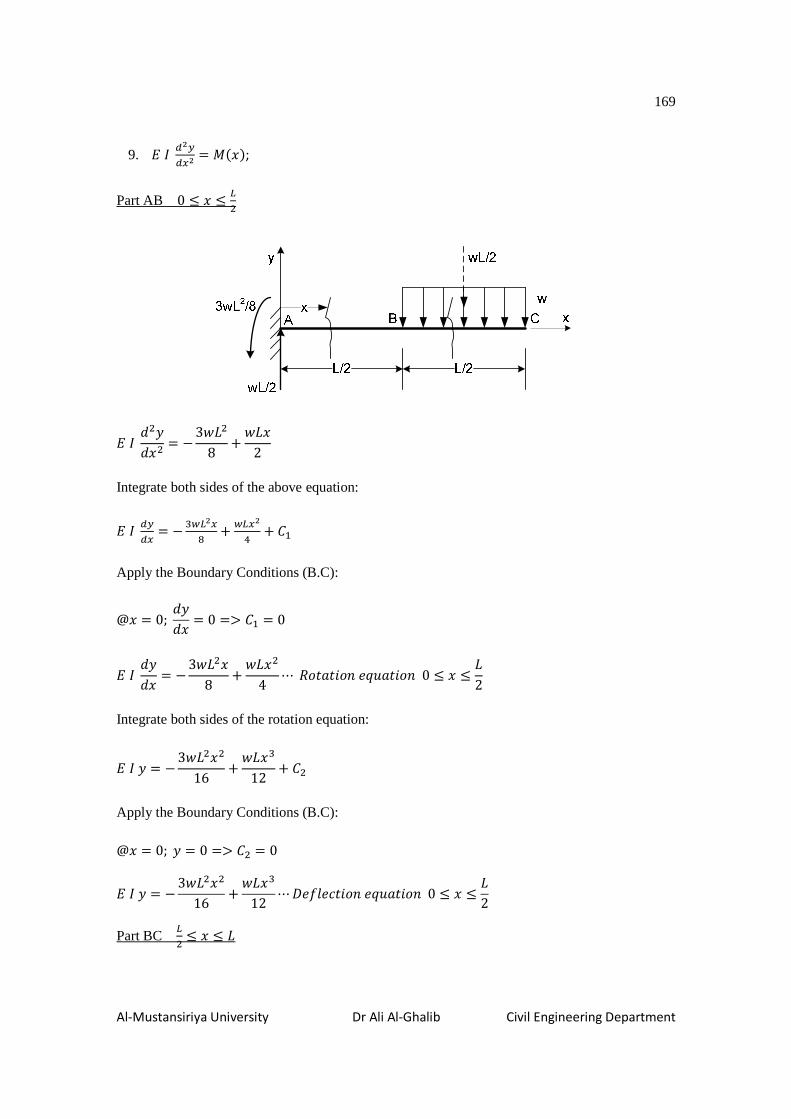
169
Al-Mustansiriya University Dr Ali Al-Ghalib Civil Engineering Department
9. lÐ &# &�# � (6n7; Part AB 0 ≤ n ≤ k�
lÐ !�g!n� � U3^j�8 + ^jn2
Integrate both sides of the above equation:
lР& &� � U HXk#� � Xk�# � �� Apply the Boundary Conditions (B.C):
@n � 0; !g!n � 0 => �� = 0
lÐ !g!n � U3^j�n8 + ^jn�4 ⋯ @]T<Tb]\`_[<Tb]\0 ≤ n ≤ j2
Integrate both sides of the rotation equation:
lÐg � U3^j�n�16 + ^jnH
12 + ��
Apply the Boundary Conditions (B.C):
@n = 0; g � 0 => �� = 0
lÐg � U3^j�n�16 + ^jnH
12 ⋯ ë`fc`dTb]\`_[<Tb]\0 ≤ n ≤ j2 Part BC
k� ≤ n ≤ j

170
Al-Mustansiriya University Dr Ali Al-Ghalib Civil Engineering Department
lÐ !�g!n� � U3^j�8 + ^jn2 − 2 (n − j2)�
Integrate both sides of the above equation:
lÐ & &� � U HXk#� � Xk�# U X� ��4H U k�#� � k#� � � �H⋯⋯63)
Apply the Continuity Condition:
@�]b\TÑ6n � j2); !g!n |�) � !g!n |)?
lÐ !g!n7) � U3^j� ∗ k�8 + ^j(k�)�4
lÐ !g!n7) � U^jH8 a[�aTbT[T`T�bab\`_63) lÐ6U^jH8lÐ) = − 3^jH
16 + ^jH16 − ^jH
48 + �H
�H = ^jH48
lÐ !g!n � U3^j�n8 + ^jn�4 − 2 ûnH
3 − jn�2 + j�n4 ý + ^jH
48 @]T<Tb]\`_[<Tb]\ j2 ≤ n ≤ j
Integrate both sides of the rotation equation:
lÐg � U3^j�n�16 + ^jnH
12 − 2 ûn 12 − jnH
6 + j�n�8 ý + ^jHn48 + � ⋯ ⋯ (4)
Apply the Continuity Conditions:
@�]b\TÑ6n � j2); g|�) � g|)?
lÐg7) � U 3^j� ∗ (k�)�16 + ^j(k�)H
12
lÐg7) � U 7^j 192lÐ a[�aTbT[T`T�bab\`_64)
lÐ6U |Xk%���qÓ7 � U HXk#6�#7#�= � Xk6�#74�� U X� û6�#7%�� U k6�#74= � k#6�#7# ý � Xk46�#7 � �
� � ^j 248

171
Al-Mustansiriya University Dr Ali Al-Ghalib Civil Engineering Department
lÐg � U 3^j�n�16 + ^jnH
12 − 2 ûn 12 − jnH
6 + j�n�8 ý + ^jHn48 + ^j
248 ë`fc`dTb]\`_[<Tb]\ j2 ≤ n ≤ j
10. lÐ &# &�# � (6n7
A
P
BC
a a
2Pa
P
EI1 EI2
x
y
x
Part AB 0 ≤ n ≤ <
l� &# &�# � U2�< + �n
Integrate both sides of the above equation:
l� & &� � U2�<n + P�#� + ��
Apply the Boundary Conditions (B.C):
@n = 0; !g!n � 0 => �� = 0
!g!n � U2�<nlÐ� � �n�2lÐ� ⋯@]T<Tb]\`_[<Tb]\0 ≤ n ≤ <
Integrate both sides of the rotation equation:
g = − �<n�lÐ� � �nH6lÐ� � ��
Apply the Boundary Conditions (B.C):
@n � 0; g � 0 => �� = 0
g = − �<n�lÐ� � �nH6lÐ�⋯ë`fc`dTb]\`_[<Tb]\0 ≤ n ≤ <

172
Al-Mustansiriya University Dr Ali Al-Ghalib Civil Engineering Department
Part BC < ≤ n ≤ 2<
l� !�g!n� � U2�< + �n
Integrate both sides of the above equation:
& &� � U �PB�qÓ# � P�#�qÓ# � �H g � U�<n�lÐ� � �nH6lÐ� � �Hn � �
Apply the First Continuity Conditions:
@�]b\TÑ;!g!nZ�) � !g!nZ)?
f]e�<eTÑ:¡!g!n¢) � U 2�<�lÐ� � �<�2lÐ� � U 3�<�
2lÐ� f]e�<eTÑ�:¡!g!n¢) � U2�<�
l� � �<�2l� � �H � U 3�<�2l� � �H
U 3�<�2l� � U 3�<�
2l� � �H �W �H � U3�<�2l� � 3�<�
2l�
Apply the Second Continuity Condition:
@�]b\TÑ;gZ�) � gZ)?
f]e�<eTÑ:YgZ) � U�<HlÐ� � �<H6lÐ� � U5�<H6lÐ�
f]e�<eT�:YgZ) � U�<Hl� � �<H6l� U 3�<H2l� � 3�<H
2l� � �
U 5�<H6l� � 2�<H
3l� U 3�<H2l� � �
� � 2�<H3l� U 2�<H
3l�
g � U�<n�l� � �nH6l� U 3�<�n2l� � 3�<�n2l� � 2�<H3l� U 2�<H
3lÐ�⋯ë`fc`dTb]\`_[<Tb]\< ≤ n ≤ 2<
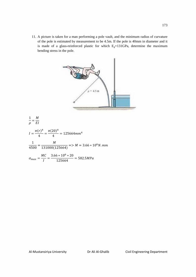
173
Al-Mustansiriya University Dr Ali Al-Ghalib Civil Engineering Department
11. A picture is taken for a man performing a pole vault, and the minimum radius of curvature of the pole is estimated by measurement to be 4.5m. If the pole is 40mm in diameter and it is made of a glass-reinforced plastic for which Eg=131GPa, determine the maximum bending stress in the pole.
1¦ = (lÐ Ð = R(e)
4 = R(20) 4 = 125664JJ
14500 = (131000(125664) => ( = 3.66 ∗ 10=I. JJ
�8B� = (�Ð = 3.66 ∗ 10= ∗ 20125664 = 582.5(�<

174
Al-Mustansiriya University Dr Ali Al-Ghalib Civil Engineering Department
Homework
For the beams loaded as shown in the figures below, determine the equation of rotation and equation of deflection.
1. Answer: g � Xk#�#=qÓ U Xk�4��qÓ � X����3kqÓ
2.
3.
12. Determine the slope and deflection at point C of the cantilever beam shown below. Take E=12GPa, and I=1.0667x109mm4.

175
Al-Mustansiriya University Dr Ali Al-Ghalib Civil Engineering Department
Solution: If the uniformly partially distributed load is extended virtually to cover the whole span, the added uniform load must be balanced by same load of opposite direction, as shown below:
(6n7 � U63 + 16n − 2n ∗ �� + 2(n − 3) ∗ (�LH)� − 4(n − 4.5)
lÐ !�g!n� = −63 + 16n − n� + (n − 3)� − 4(n − 4.5)
lÐ !g!n = −63n + 8n� − nH3 + (n − 3)H
3 − 2(n − 4.5)� + ��
lÐg = − 63n�2 + 8nH
3 − n 12 + (n − 3)
12 − 2 (n − 4.5)H3 + ��
Apply the first Boundary Conditions (B.C):
@n = 0; !g!n � 0 => �� = 0
Apply the second Boundary Conditions (B.C):
@n = 0; g � 0 => �� = 0

176
Al-Mustansiriya University Dr Ali Al-Ghalib Civil Engineering Department
!g!n |� � §� � 1lÐ ²−63 ∗ 6 + 8 ∗ 6� − 6H3 + (6 − 3)H
3 − 2(6 − 4.5)�³ = −157.5NI. J� ∗ 10�12 ∗ 10H ∗ 1.0667 ∗ 10�
= −0.0123e<!
g� = ∆�= 1lÐ ²− 63 ∗ 6�2 + 8 ∗ 6H
3 − 6 12 + (6 − 3)
12 − 2 (6 − 4.5)H3 ³ = −661.5NI. JH ∗ 10��
12 ∗ 10H ∗ 1.0667 ∗ 10�= −51.7JJ