Embed Size (px)
Citation preview
Mechanics of Machines
Dr. Mohammad Kilani
Class 3Position Analysis
TYPES OF MECHANISM ANALYSESE
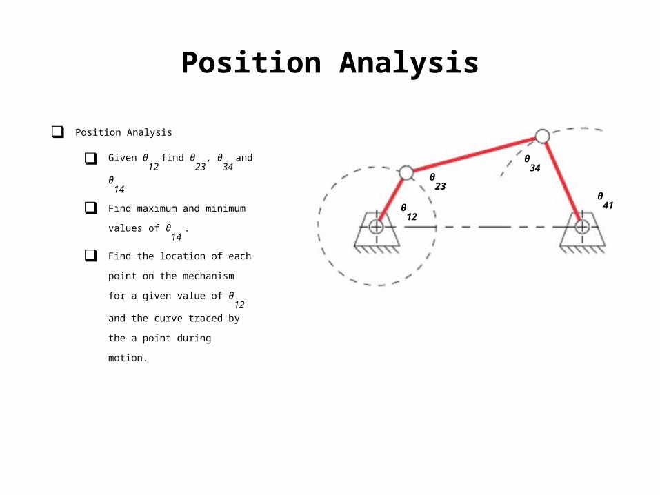
Position Analysis
Position Analysis
Given θ12
find θ23
, θ34
and θ14
Find maximum and minimum values
of θ14
.
Find the location of each point on
the mechanism for a given value of
θ12
and the curve traced by the a
point during motion.
θ12
θ41
θ23
θ34
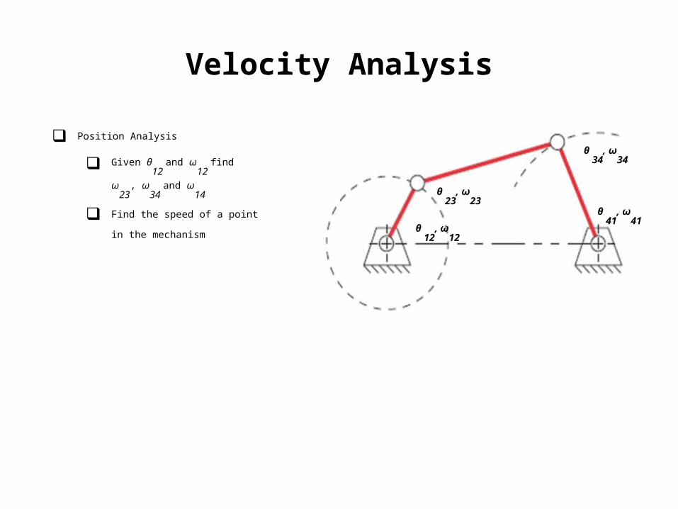
Velocity Analysis
Position Analysis
Given θ12
and ω12
find ω23
, ω34
and ω14
Find the speed of a point in the
mechanismθ
12, ω
12
θ 23
, ω23
θ 34
, ω34
θ 41
, ω41
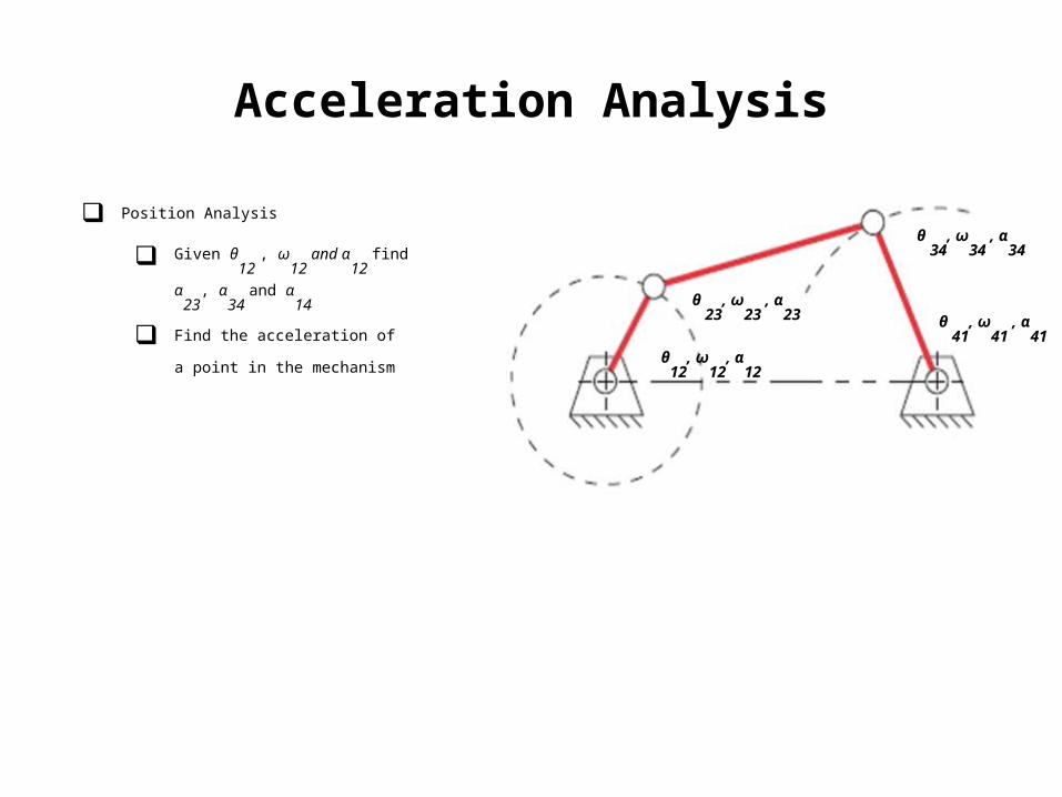
Acceleration Analysis
Position Analysis
Given θ12
, ω12
and α12
find α23
,
α34
and α14
Find the acceleration of a point in the
mechanismθ
12, ω
12, α
12
θ 23
, ω23
, α23
θ 34
, ω34
, α34
θ 41
, ω41
, α41
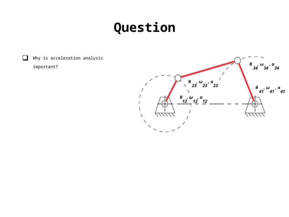
Question
Why is acceleration analysis important?
θ12
, ω12
, α12
θ 23
, ω23
, α23
θ 34
, ω34
, α34
θ 41
, ω41
, α41

GRAPHICAL POSITION ANALYSIS
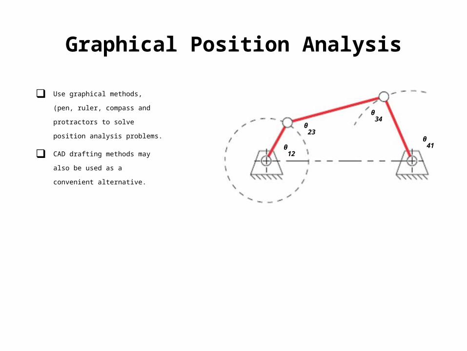
Graphical Position Analysis
Use graphical methods, (pen, ruler,
compass and protractors to solve
position analysis problems.
CAD drafting methods may also be used
as a convenient alternative.θ
12
θ41
θ23
θ34
VECTOR POSITION ANALYSIS
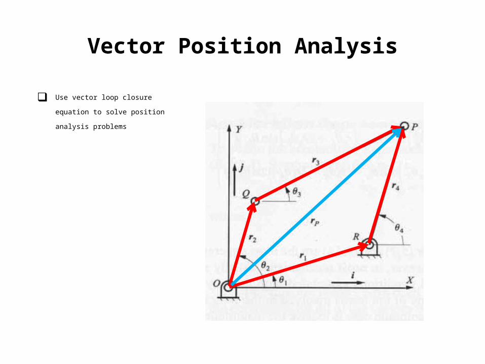
Vector Position Analysis
Use vector loop closure equation to
solve position analysis problems
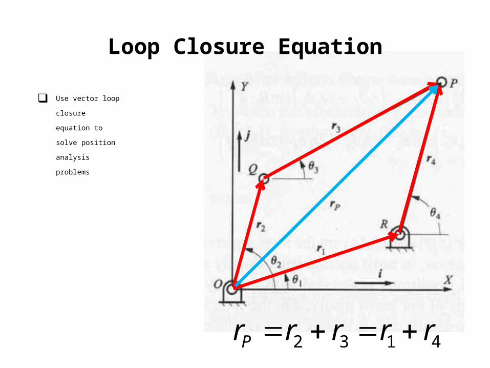
Loop Closure Equation
Use vector loop
closure equation to
solve position analysis
problems
4132 rrrrrP
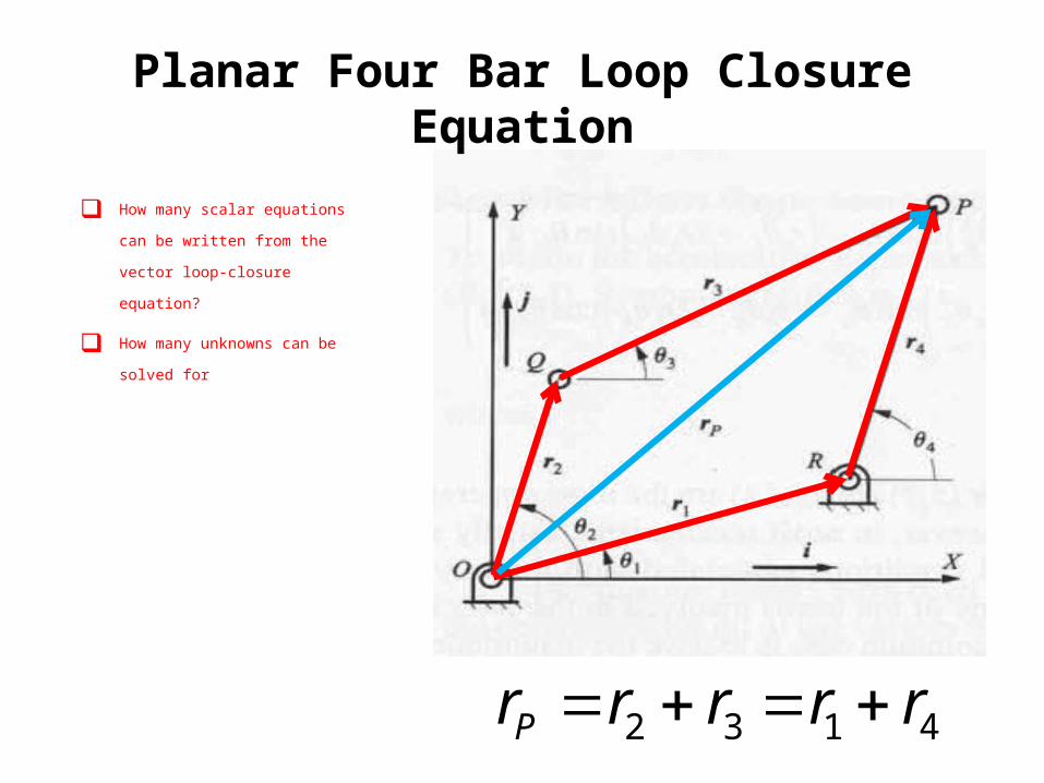
Planar Four Bar Loop Closure Equation
How many scalar equations can be
written from the vector loop-closure
equation?
How many unknowns can be solved for
4132 rrrrrP
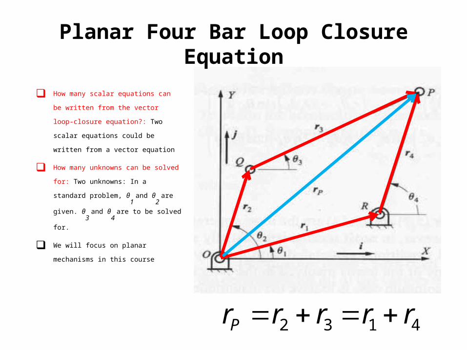
Planar Four Bar Loop Closure Equation
How many scalar equations can be written
from the vector loop-closure equation?: Two
scalar equations could be written from a
vector equation
How many unknowns can be solved for: Two
unknowns: In a standard problem, θ1
and θ2
are given. θ3
and θ4
are to be solved for.
We will focus on planar mechanisms in this
course
4132 rrrrrP
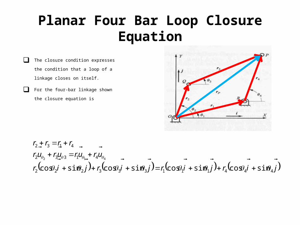
Planar Four Bar Loop Closure Equation
The closure condition expresses the condition
that a loop of a linkage closes on itself.
For the four-bar linkage shown the closure
equation is
jirjirjirjir
urururur
rrrr
444111333222
41332
4132
sincossincossincossincos
412
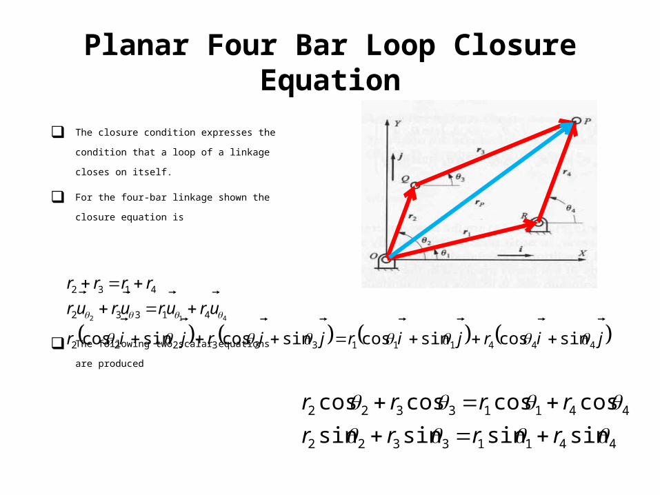
Planar Four Bar Loop Closure Equation
The closure condition expresses the condition that a
loop of a linkage closes on itself.
For the four-bar linkage shown the closure equation is
The following two scalar equations are produced
jirjirjirjir
urururur
rrrr
444111333222
41332
4132
sincossincossincossincos
412
44113322
44113322
sinsinsinsin
coscoscoscos
rrrr
rrrr
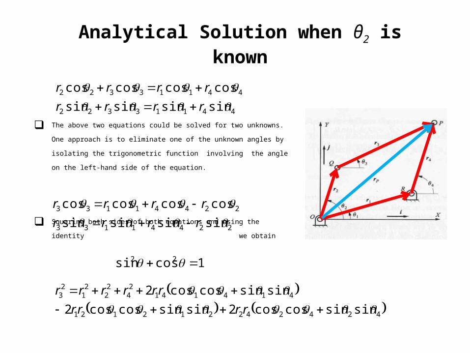
Analytical Solution when θ2 is known
The above two equations could be solved for two unknowns. One approach is to
eliminate one of the unknown angles by isolating the trigonometric function involving
the angle on the left-hand side of the equation.
Squaring both sides of both equations and using the identity we
obtain
44113322
44113322
sinsinsinsin
coscoscoscos
rrrr
rrrr
22441133
22441133
sinsinsinsin
coscoscoscos
rrrr
rrrr
1cossin 22
424242212121
41414124
22
21
23
sinsincoscos2sinsincoscos2
sinsincoscos2
rrrr
rrrrrr
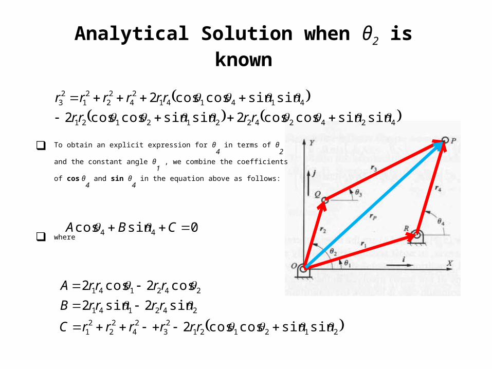
Analytical Solution when θ2 is known
To obtain an explicit expression for θ4
in terms of θ2
and the constant angle θ1
,
we combine the coefficients of cos θ4
and sin θ4
in the equation above as
follows:
where
21212123
24
22
21
242141
242141
sinsincoscos2
sin2sin2
cos2cos2
rrrrrrC
rrrrB
rrrrA
424242212121
41414124
22
21
23
sinsincoscos2sinsincoscos2
sinsincoscos2
rrrr
rrrrrr
0sincos 44 CBA
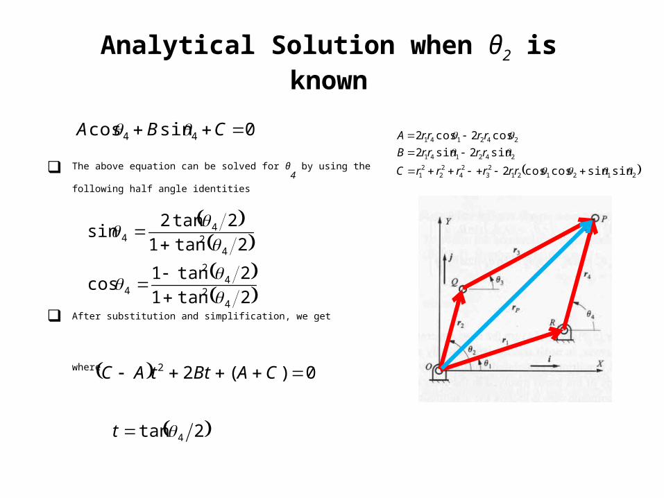
The above equation can be solved for θ4
by using the following half angle
identities
After substitution and simplification, we get
where
21212123
24
22
21
242141
242141
sinsincoscos2
sin2sin2
cos2cos2
rrrrrrC
rrrrB
rrrrA0sincos 44 CBA
2tan1
2tan1cos
2tan1
2tan2sin
42
42
4
424
4
0)(22 CABttAC
2tan 4t
Analytical Solution when θ2 is known
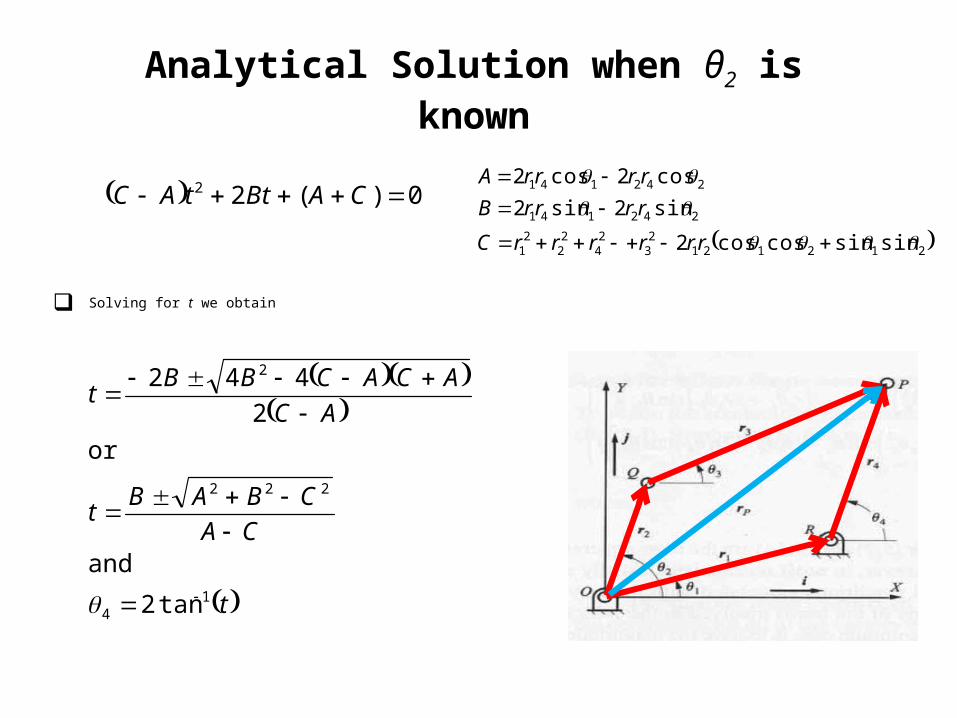
Solving for t we obtain
21212123
24
22
21
242141
242141
sinsincoscos2
sin2sin2
cos2cos2
rrrrrrC
rrrrB
rrrrA 0)(22 CABttAC
t
CA
CBABt
AC
ACACBBt
14
222
2
tan2
2
442
and
or
Analytical Solution when θ2 is known
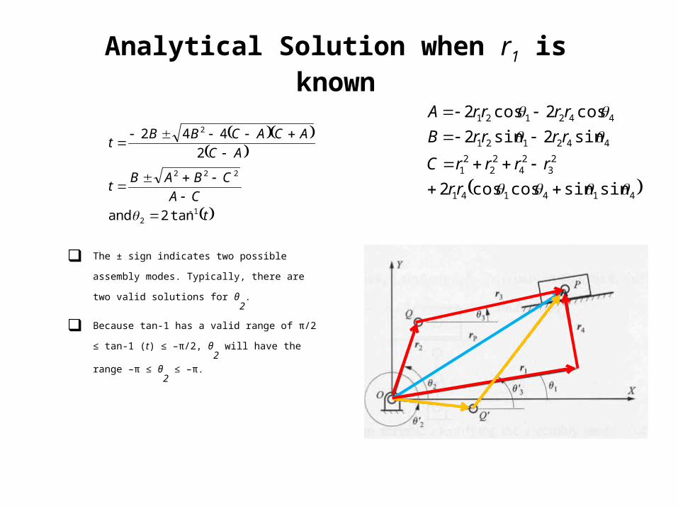
The ± sign identifies the two possible assembly modes of the linkage
t
CA
CBABt
rr
rrrrC
rrrrB
rrrrA
14
222
212121
23
24
22
21
242141
242141
tan2
sinsincoscos2
sin2sin2
cos2cos2
and
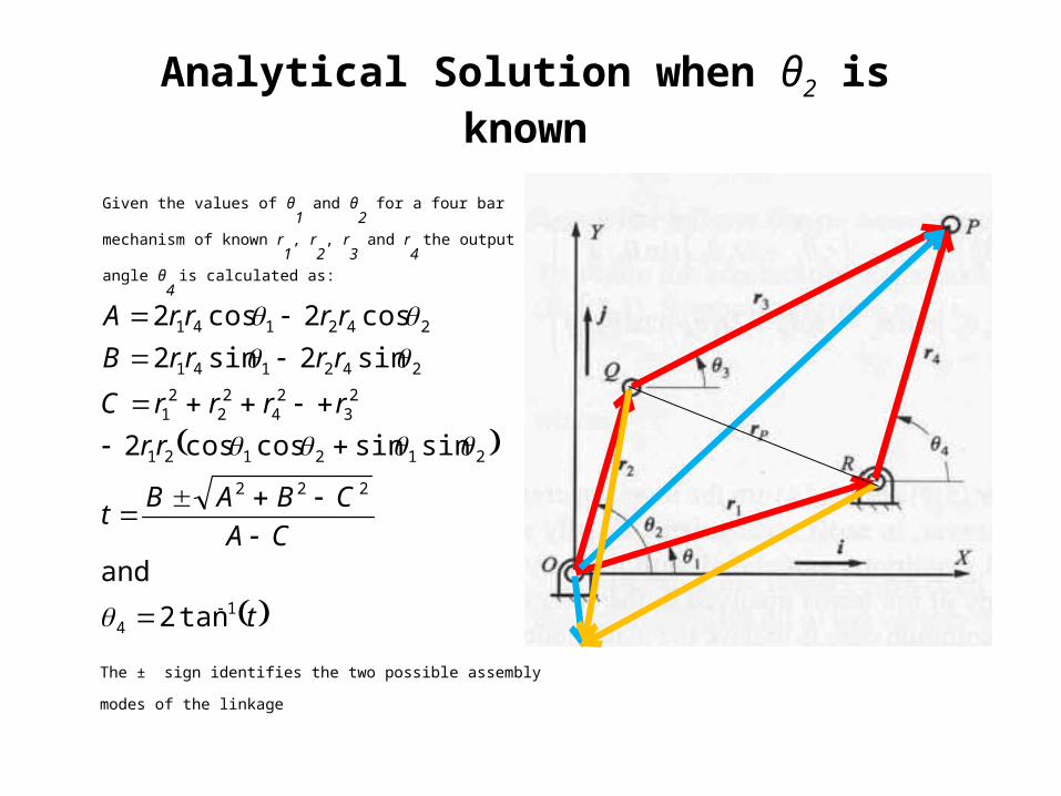
Given the values of θ1
and θ2
for a four bar mechanism of known r1
,
r2
, r3
and r4
the output angle θ4
is calculated as:
Analytical Solution when θ2 is known
The ± sign identifies the two possible assembly modes of the linkage
t
CA
CBABt
rr
rrrrC
rrrrB
rrrrA
14
222
212121
23
24
22
21
242141
242141
tan2
sinsincoscos2
sin2sin2
cos2cos2
and
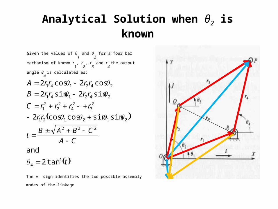
Given the values of θ1
and θ2
for a four bar mechanism of known r1
,
r2
, r3
and r4
the output angle θ4
is calculated as:
Analytical Solution when θ2 is known
t
CA
CBABt
rr
rrrrC
rrrrB
rrrrA
14
222
212121
23
24
22
21
242141
242141
tan2
sinsincoscos2
sin2sin2
cos2cos2
and
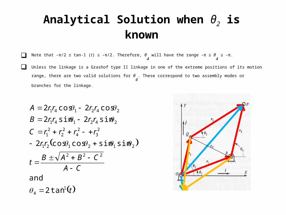
Note that –π/2 ≤ tan-1 (t) ≤ –π/2. Therefore, θ4
will have the range –π ≤ θ4
≤ –π.
Unless the linkage is a Grashof type II linkage in one of the extreme positions of its motion range, there are two valid solutions for θ4
.
These correspond to two assembly modes or branches for the linkage.
Analytical Solution when θ2 is known
t
CA
CBABt
rr
rrrrC
rrrrB
rrrrA
14
222
212121
23
24
22
21
242141
242141
tan2
sinsincoscos2
sin2sin2
cos2cos2
and
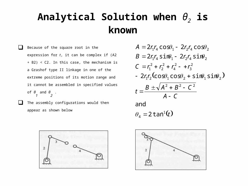
Because of the square root in the expression for t, it can be
complex if (A2 + B2) < C2. In this case, the mechanism is a
Grashof type II linkage in one of the extreme positions of its
motion range and it cannot be assembled in specified values of
θ1
and θ2
.
The assembly configurations would then appear as shown
below
Analytical Solution when θ2 is known
t
CA
CBABt
rr
rrrrC
rrrrB
rrrrA
14
222
212121
23
24
22
21
242141
242141
tan2
sinsincoscos2
sin2sin2
cos2cos2
and
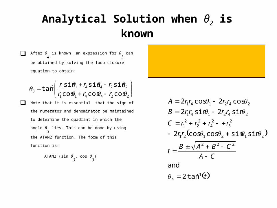
After θ4
is known, an expression for θ3
can be obtained by
solving the loop closure equation to obtain:
Note that it is essential that the sign of the numerator and
denominator be maintained to determine the quadrant in
which the angle θ3
lies. This can be done by using the ATAN2
function. The form of this function is:
ATAN2 (sin θ3
, cos θ3
)
22441133
22441133
sinsinsinsin
coscoscoscos
rrrr
rrrr
224411
22441113 coscoscos
sinsinsintan
rrr
rrr
Analytical Solution when θ2 is known
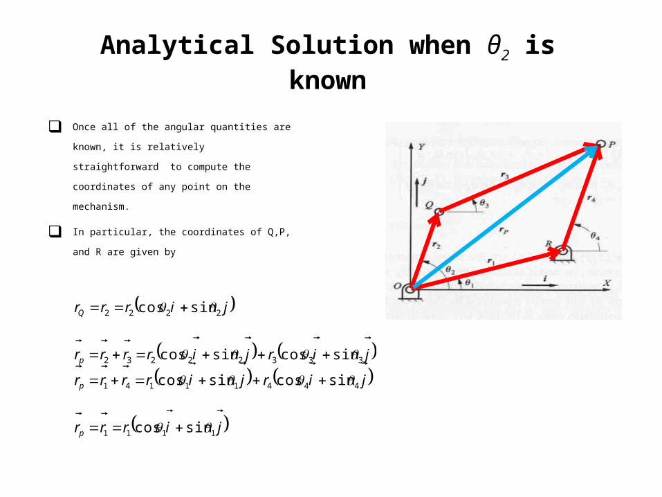
Once all of the angular quantities are known, it is
relatively straightforward to compute the coordinates
of any point on the mechanism.
In particular, the coordinates of Q,P, and R are given by
jirrr
jirjirrrr
jirjirrrr
jirrr
p
p
p
Q
1111
44411141
33322232
2222
sincos
sincossincos
sincossincos
sincos
Analytical Solution when θ2 is known
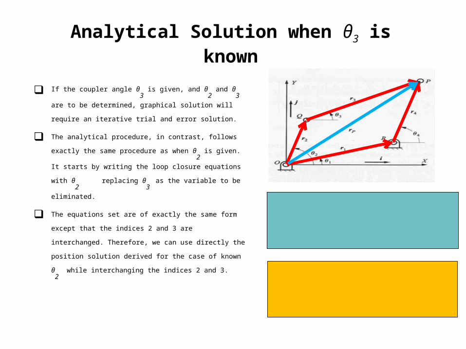
If the coupler angle θ3
is given, and θ2
and θ3
are to be determined,
graphical solution will require an iterative trial and error solution.
The analytical procedure, in contrast, follows exactly the same
procedure as when θ2
is given. It starts by writing the loop closure
equations with θ2
replacing θ3
as the variable to be
eliminated.
The equations set are of exactly the same form except that the indices
2 and 3 are interchanged. Therefore, we can use directly the position
solution derived for the case of known θ2
while interchanging the
indices 2 and 3.
Analytical Solution when θ3 is known
33441122
33441122
sinsinsinsin
coscoscoscos
rrrr
rrrr
22441133
22441133
sinsinsinsin
coscoscoscos
rrrr
rrrr
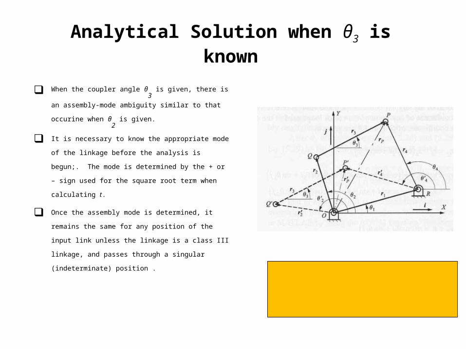
When the coupler angle θ3
is given, there is an assembly-mode
ambiguity similar to that occurine when θ2
is given.
It is necessary to know the appropriate mode of the linkage
before the analysis is begun;. The mode is determined by the +
or – sign used for the square root term when calculating t.
Once the assembly mode is determined, it remains the same for
any position of the input link unless the linkage is a class III
linkage, and passes through a singular (indeterminate) position .
Analytical Solution when θ3 is known
33441122
33441122
sinsinsinsin
coscoscoscos
rrrr
rrrr
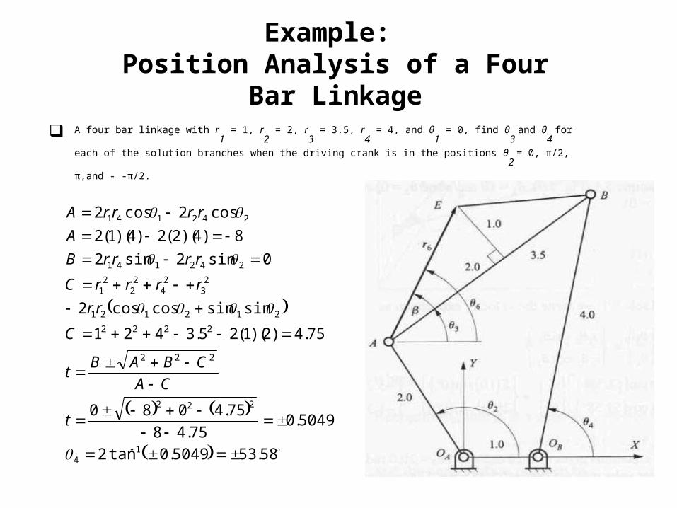
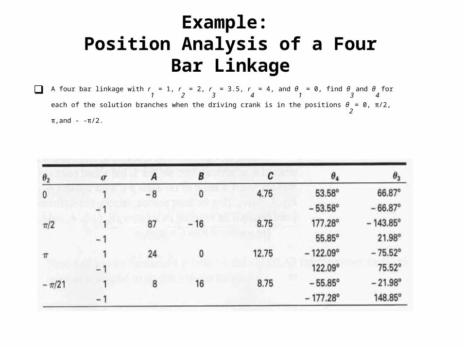
A four bar linkage with r1
= 1, r2
= 2, r3
= 3.5, r4
= 4, and θ1
= 0, find θ3
and θ4
for each of the solution branches when the
driving crank is in the positions θ2
= 0, π/2, π,and - -π/2.
Example: Position Analysis of a Four Bar Linkage
58.535049.0tan2
5049.075.48
75.4080
75.4)2)(1(25.3421
sinsincoscos2
0sin2sin2
8)4)(2(2)4)(1(2
cos2cos2
14
222
222
2222
212121
23
24
22
21
242141
242141
t
CA
CBABt
C
rr
rrrrC
rrrrB
A
rrrrA
A four bar linkage with r1
= 1, r2
= 2, r3
= 3.5, r4
= 4, and θ1
= 0, find θ3
and θ4
for each of the solution branches when the driving
crank is in the positions θ2
= 0, π/2, π,and - -π/2.
Example: Position Analysis of a Four Bar Linkage
POSITION ANALYSIS FOR A RIGID BODY WHEN TWO POINTS ARE KNOWN
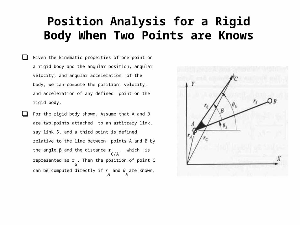
Given the kinematic properties of one point on a rigid body and the
angular position, angular velocity, and angular acceleration of the
body, we can compute the position, velocity, and acceleration of any
defined point on the rigid body.
For the rigid body shown. Assume that A and B are two points
attached to an arbitrary link, say link 5, and a third point is defined
relative to the line between points A and B by the angle β and the
distance rC/A
, which is represented as r6
. Then the position of point
C can be computed directly if rA
and θ5
are known.
Position Analysis for a Rigid Body When Two Points are Knows
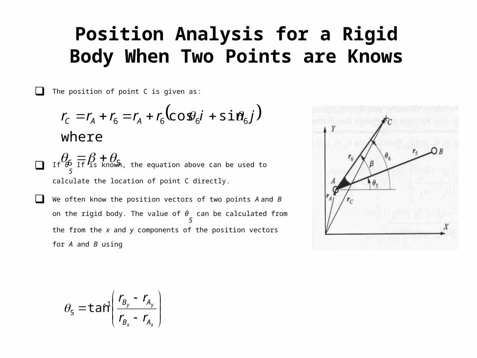
The position of point C is given as:
If θ5
If is known, the equation above can be used to calculate the location of point
C directly.
We often know the position vectors of two points A and B on the rigid body. The
value of θ5
can be calculated from the from the x and y components of the position
vectors for A and B using
Position Analysis for a Rigid Body When Two Points are Knows
56
6666 sincos
where
jirrrrr AAC
xx
yy
AB
AB
rr
rr1
5 tan
POSITION ANALYSIS FOR A SLIDER-CRANK MECHANISM
HW#2 (Prob. 4-6 and 4-7, with data in row (a)
Table P4-1).(4-10, 4-12, 4-18(f))
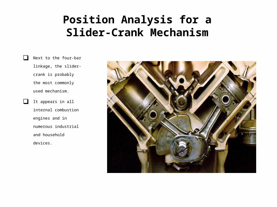
Next to the four-bar linkage,
the slider-crank is probably
the most commonly used
mechanism.
It appears in all internal
combustion engines and in
numerous industrial and
household devices.
Position Analysis for a Slider-Crank Mechanism
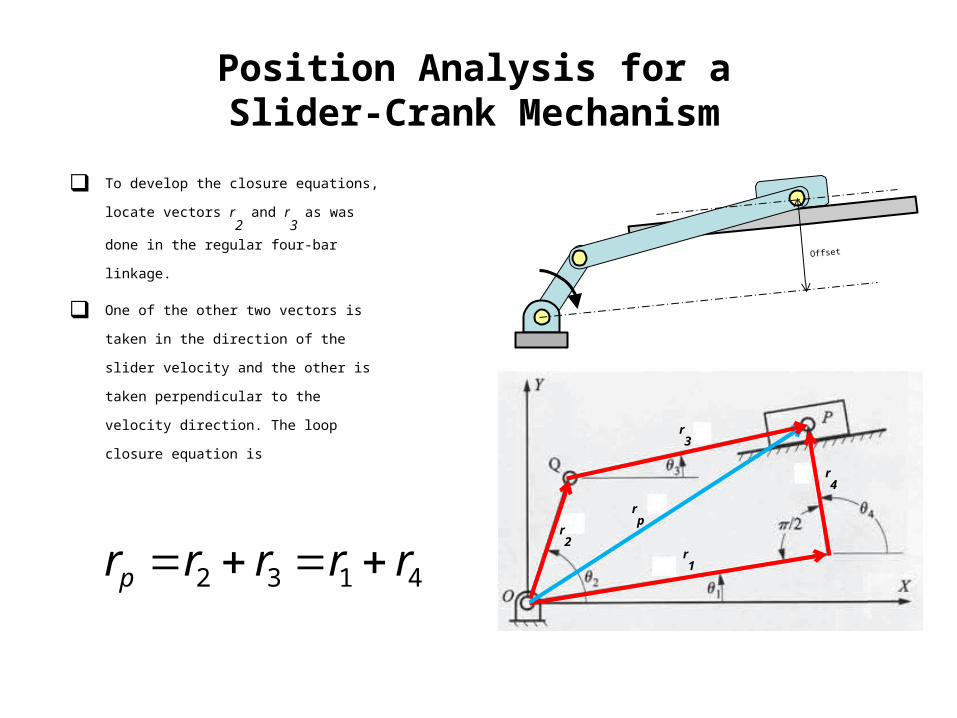
To develop the closure equations, locate vectors
r2
and r3
as was done in the regular four-bar
linkage.
One of the other two vectors is taken in the
direction of the slider velocity and the other is
taken perpendicular to the velocity direction.
The loop closure equation is
Position Analysis for a Slider-Crank Mechanism
4132 rrrrrp
Offset
r3
r2
r1
r4
rp
Position Analysis for a Slider-Crank Mechanism
2
sincossincos
sincossincos
14
444111
333222
41332
4132
412
wherejirjir
jirjir
urururur
rrrr
44113322
44113322
sinsinsinsin
coscoscoscos
rrrr
rrrr
Writing the loop closure equation in terms of the
vector angles, we obtain
Two scalar equations are produced. The equations
can be solved for two unknowns.
r3
r2
r1
r4
rp
Position Analysis for a Slider-Crank Mechanism
44113322
44113322
sinsinsinsin
coscoscoscos
rrrr
rrrr
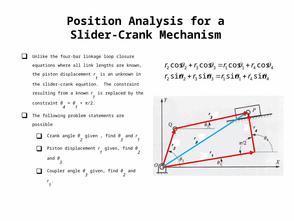
Unlike the four-bar linkage loop closure equations where all link
lengths are known, the piston displacement r1
is an unknown in
the slider-crank equation. The constraint resulting from a
known r1
is replaced by the constraint θ4
= θ1
+ π/2.
The following problem statements are possible
Crank angle θ2
given , find θ3
and r1
Piston displacement r1
given, find θ2
and θ3
Coupler angle θ3
given, find θ2
and r1
.
r3
r2
r1
r4
rp
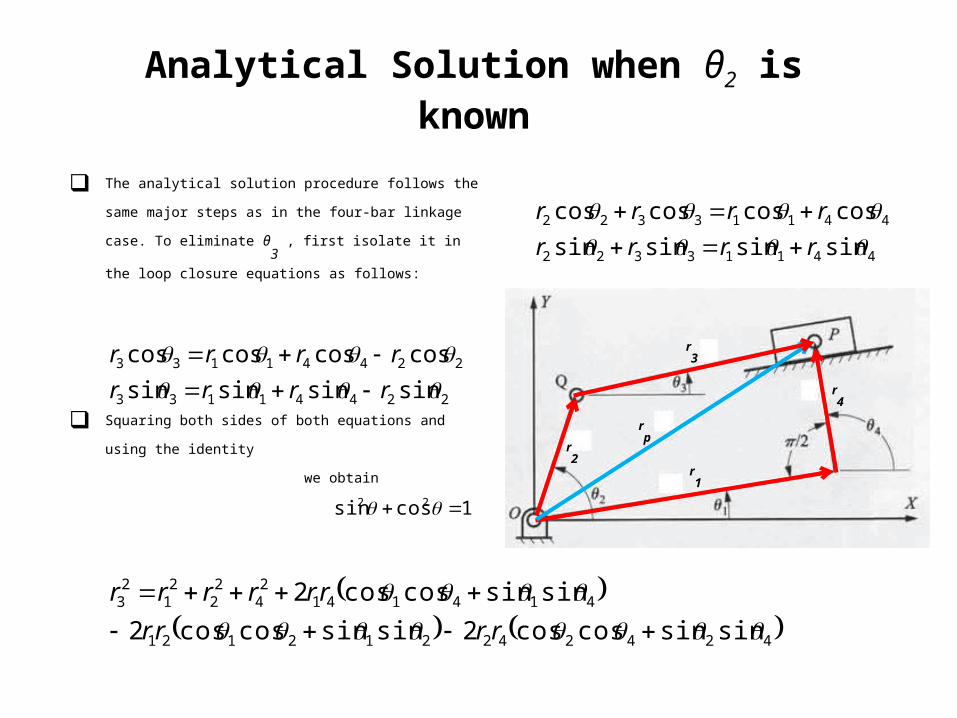
Analytical Solution when θ2 is known
44113322
44113322
sinsinsinsin
coscoscoscos
rrrr
rrrr
The analytical solution procedure follows the same major steps as
in the four-bar linkage case. To eliminate θ3
, first isolate it in the
loop closure equations as follows:
Squaring both sides of both equations and using the identity
we obtain
r3
r2
r1
r4
rp
22441133
22441133
sinsinsinsin
coscoscoscos
rrrr
rrrr
1cossin 22
424242212121
41414124
22
21
23
sinsincoscos2sinsincoscos2
sinsincoscos2
rrrr
rrrrrr
Analytical Solution when θ2 is known
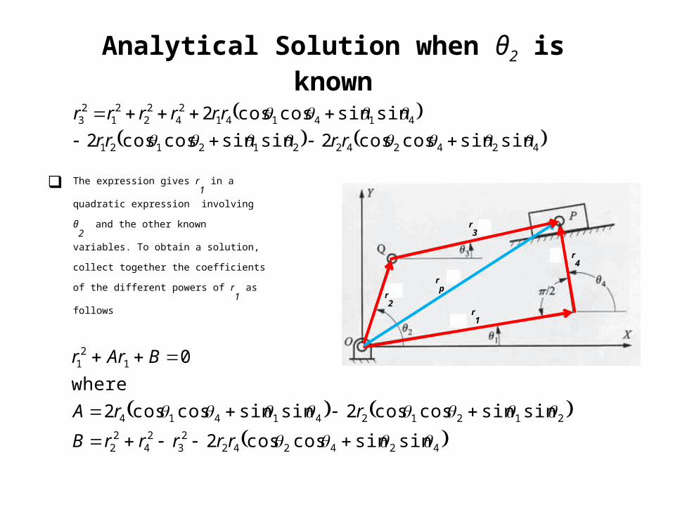
The expression gives r1
in a quadratic expression
involving θ2
and the other known variables. To
obtain a solution, collect together the
coefficients of the different powers of r1
as
follows
r3
r2
r1
r4
rp
424242212121
41414124
22
21
23
sinsincoscos2sinsincoscos2
sinsincoscos2
rrrr
rrrrrr
424242
23
24
22
2121241414
121
sinsincoscos2
sinsincoscos2sinsincoscos2
0
rrrrrB
rrA
BArr
where
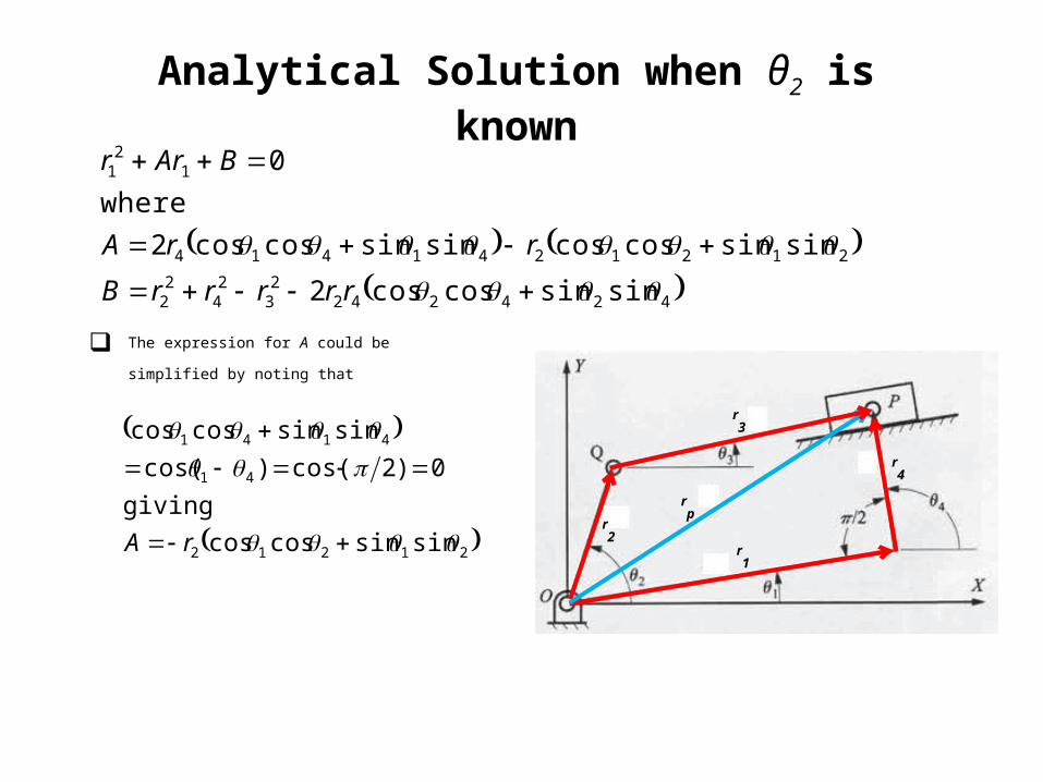
Analytical Solution when θ2 is known
r3
r2
r1
r4
rp
424242
23
24
22
2121241414
121
sinsincoscos2
sinsincoscossinsincoscos2
0
rrrrrB
rrA
BArr
where
21212
41
4141
sinsincoscos
0)2cos()cos(
sinsincoscos
rA
giving
The expression for A could be simplified by
noting that
Analytical Solution when θ2 is known
424242
23
24
22
21212
121
sinsincoscos2
sinsincoscos
0
rr
rrrB
rA
BArr
where
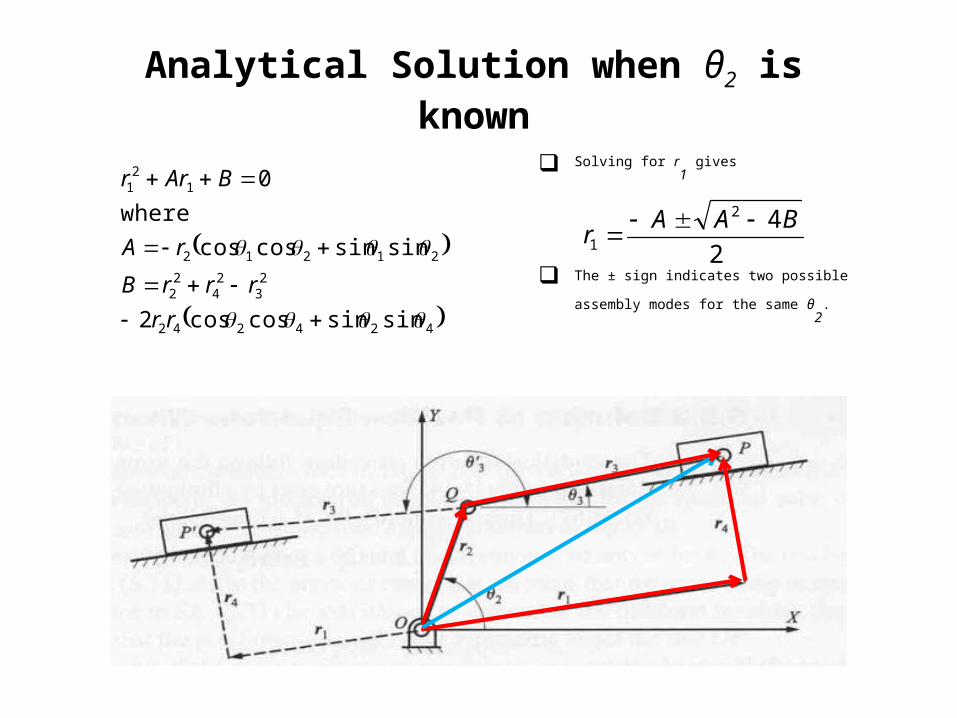
Solving for r1
gives
The ± sign indicates two possible assembly
modes for the same θ2
.
2
42
1
BAAr
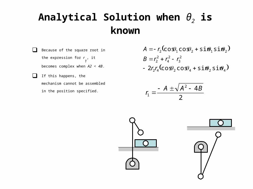
Analytical Solution when θ2 is known
424242
23
24
22
21212
sinsincoscos2
sinsincoscos
rr
rrrB
rA Because of the square root in the
expression for r1
, it becomes complex
when A2 < 4B.
If this happens, the mechanism cannot be
assembled in the position specified.
2
42
1
BAAr
Analytical Solution when θ2 is known
424242
23
24
22
21212
sinsincoscos2
sinsincoscos
rr
rrrB
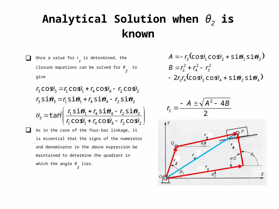
rA Once a value for r1
is determined, the closure equations can be
solved for θ3
to give
As in the case of the four-bar linkage, it is essential that the signs
of the numerator and denominator in the above expression be
maintained to determine the quadrant in which the angle θ3
lies.
2
42
1
BAAr
224411
22441113
22441133
22441133
coscoscos
sinsinsintan
sinsinsinsin
coscoscoscos
rrr
rrr
rrrr
rrrr
r3
r2
r1
r4
rp
Analytical Solution when θ2 is known
424242
23
24
22
21212
sinsincoscos2
sinsincoscos
rr
rrrB
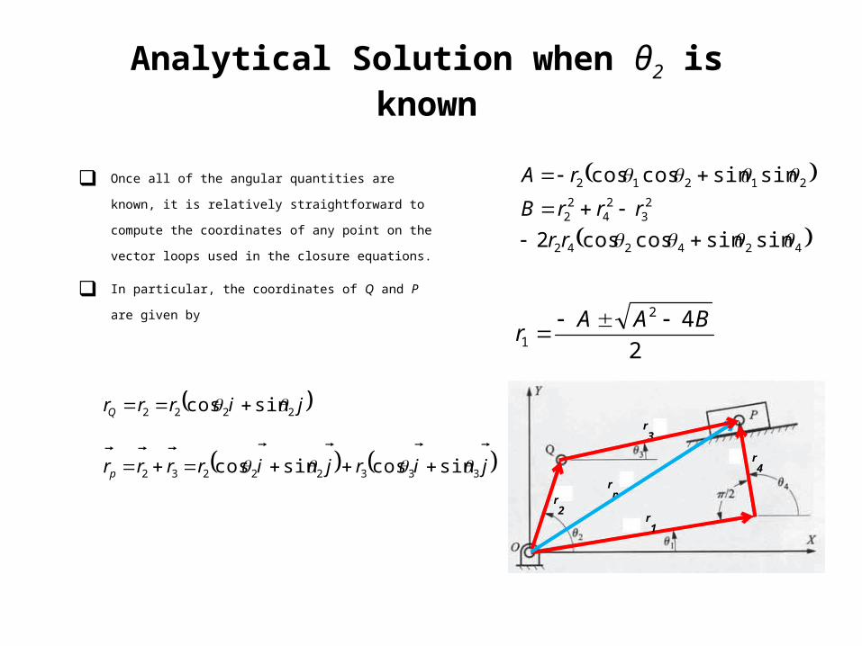
rA Once all of the angular quantities are known, it is relatively
straightforward to compute the coordinates of any point on the
vector loops used in the closure equations.
In particular, the coordinates of Q and P are given by
2
42
1
BAAr
r3
r2
r1
r4
rp
jirjirrrr
jirrr
p
Q
33322232
2222
sincossincos
sincos
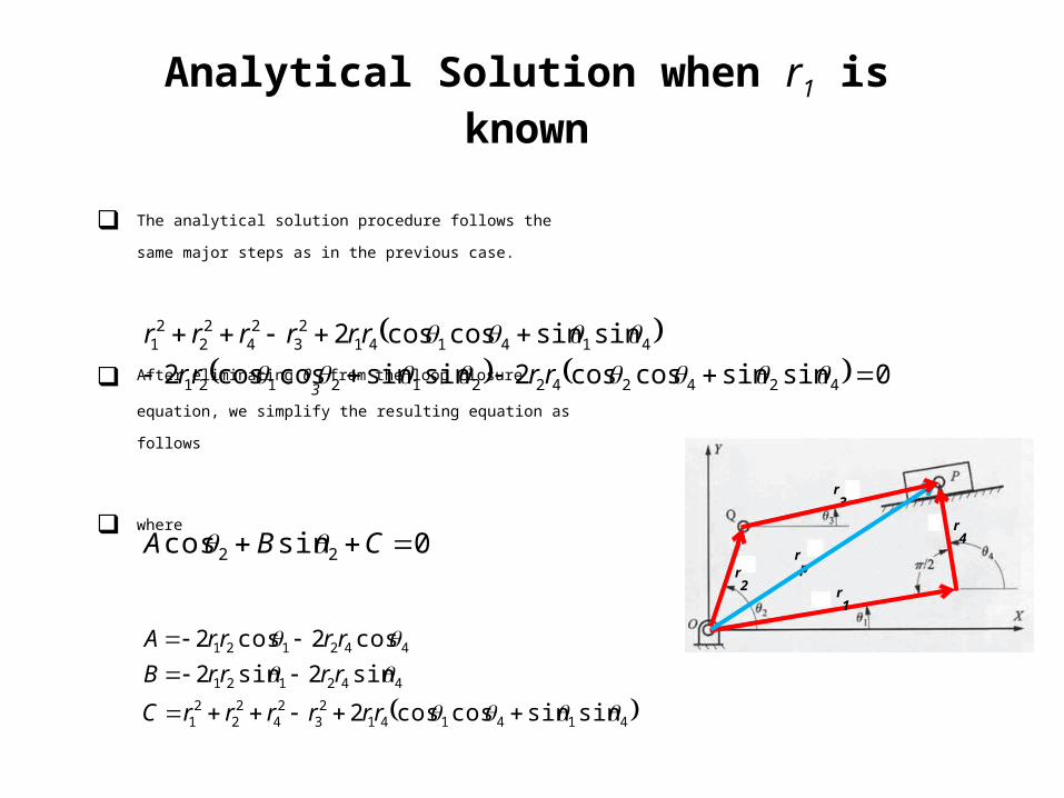
Analytical Solution when r1 is known
The analytical solution procedure follows the same major steps as in
the previous case.
After eliminating θ3
from the loop closure equation, we simplify the
resulting equation as follows
where r3
r2 r
1
r4
rp
0sincos 22 CBA
0sinsincoscos2sinsincoscos2
sinsincoscos2
424242212121
41414123
24
22
21
rrrr
rrrrrr
41414123
24
22
21
442121
442121
sinsincoscos2
sin2sin2
cos2cos2
rrrrrrC
rrrrB
rrrrA
Analytical Solution when r1 is known
The trigonometric half-angle identities can be used to solve the
equation above for θ2
. Using these identities and simplifying gives
Solving for t gives
r3
r2 r
1
r4
rp
0sincos 22 CBA
414141
23
24
22
21
442121
442121
sinsincoscos2
sin2sin2
cos2cos2
rr
rrrrC
rrrrB
rrrrA
2tan1
2tan1cos
2tan1
2tan2sin
22
22
2
222
2
2tan
0)(2
2
2
t
CABttAC
where
tCA
CBABt
AC
ACACBBt
12
222
2
tan2
2
442
and
Analytical Solution when r1 is known
The ± sign indicates two possible assembly modes.
Typically, there are two valid solutions for θ2
.
Because tan-1 has a valid range of π/2 ≤ tan-1 (t) ≤ –π/2,
θ2
will have the range –π ≤ θ2
≤ –π.
414141
23
24
22
21
442121
442121
sinsincoscos2
sin2sin2
cos2cos2
rr
rrrrC
rrrrB
rrrrA
tCA
CBABt
AC
ACACBBt
12
222
2
tan2
2
442
and
Analytical Solution when r1 is known
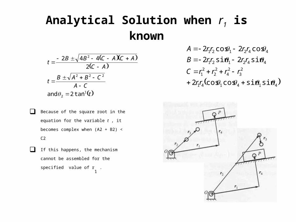
Because of the square root in the equation for the
variable t , it becomes complex when (A2 + B2) <
C2
If this happens, the mechanism cannot be
assembled for the specified value of r1
.
414141
23
24
22
21
442121
442121
sinsincoscos2
sin2sin2
cos2cos2
rr
rrrrC
rrrrB
rrrrA
tCA
CBABt
AC
ACACBBt
12
222
2
tan2
2
442
and
Analytical Solution when r1 is known
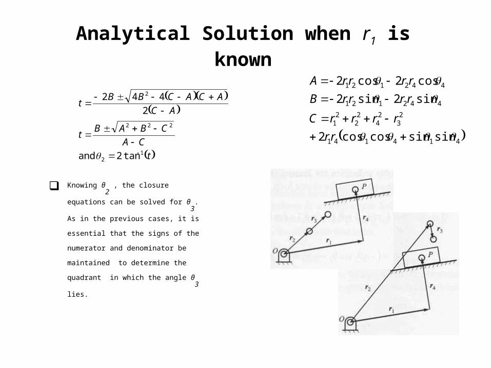
Knowing θ2
, the closure equations can be
solved for θ3
. As in the previous cases, it is
essential that the signs of the numerator and
denominator be maintained to determine the
quadrant in which the angle θ3
lies.
414141
23
24
22
21
442121
442121
sinsincoscos2
sin2sin2
cos2cos2
rr
rrrrC
rrrrB
rrrrA
tCA
CBABt
AC
ACACBBt
12
222
2
tan2
2
442
and
Analytical Solution when θ3 is known
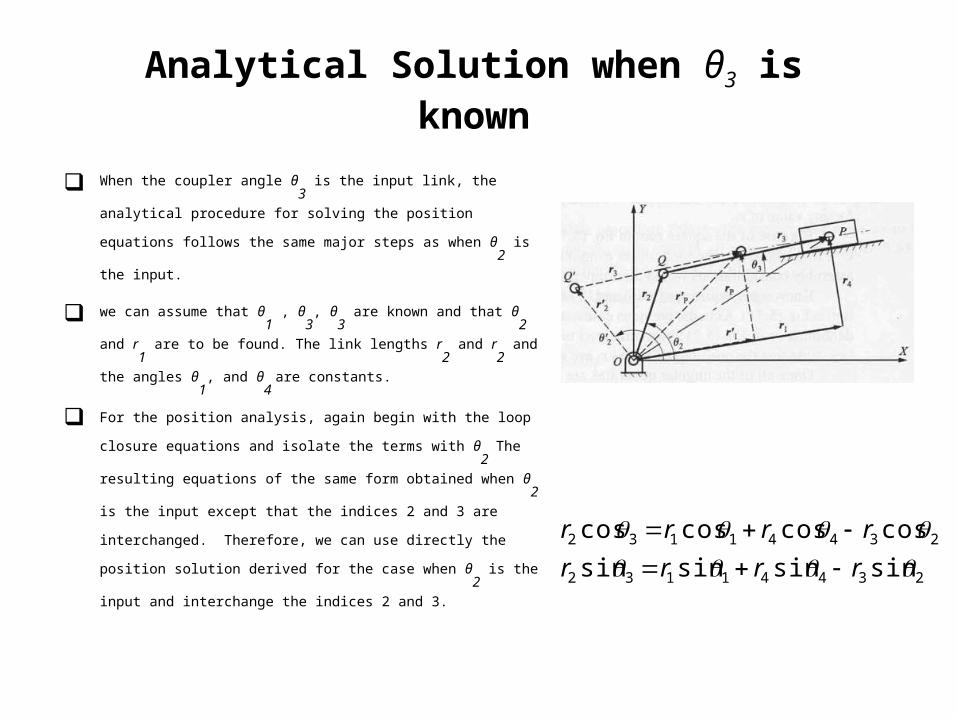
When the coupler angle θ3
is the input link, the analytical procedure for solving
the position equations follows the same major steps as when θ2
is the input.
we can assume that θ1
, θ3
, θ3
are known and that θ2
and r1
are to be found.
The link lengths r2
and r2
and the angles θ1
, and θ4
are constants.
For the position analysis, again begin with the loop closure equations and
isolate the terms with θ2
The resulting equations of the same form obtained
when θ2
is the input except that the indices 2 and 3 are interchanged.
Therefore, we can use directly the position solution derived for the case when
θ2
is the input and interchange the indices 2 and 3.
23441132
23441132
sinsinsinsin
coscoscoscos
rrrr
rrrr
POSITION ANALYSIS FOR AN INVERTED SLIDER-CRANK MECHANISM
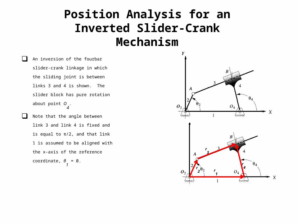
An inversion of the fourbar slider-crank linkage
in which the sliding joint is between links 3
and 4 is shown. The slider block has pure
rotation about point O4
.
Note that the angle between link 3 and link 4
is fixed and is equal to π/2, and that link 1 is
assumed to be aligned with the x-axis of the
reference coordinate, θ1
= 0.
Position Analysis for an Inverted Slider-Crank Mechanism
r3
r2 r
1
r4
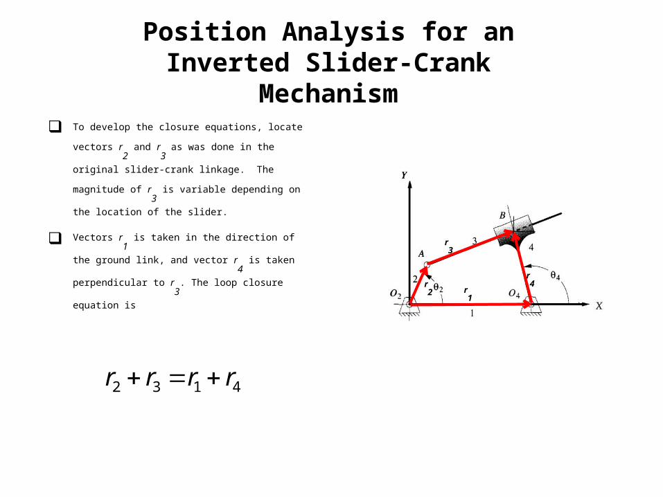
To develop the closure equations, locate vectors r2
and r3
as was done in the original slider-crank linkage. The
magnitude of r3
is variable depending on the location of
the slider.
Vectors r1
is taken in the direction of the ground link, and
vector r4
is taken perpendicular to r3
. The loop closure
equation is
Position Analysis for an Inverted Slider-Crank Mechanism
4132 rrrr
r3
r2 r
1
r4
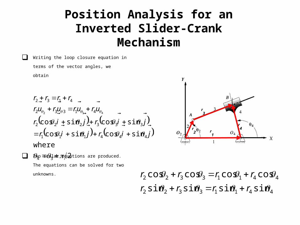
Position Analysis for an Inverted Slider-Crank Mechanism
2
sincossincos
sincossincos
34
444111
333222
41332
4132
412
wherejirjir
jirjir
urururur
rrrr
44113322
44113322
sinsinsinsin
coscoscoscos
rrrr
rrrr
Writing the loop closure equation in terms of the
vector angles, we obtain
Two scalar equations are produced. The equations
can be solved for two unknowns.
r3
r2 r
1
r4
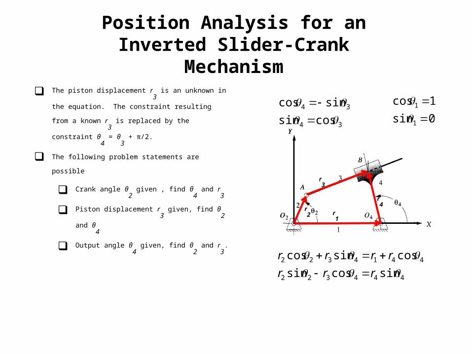
Position Analysis for an Inverted Slider-Crank Mechanism
The piston displacement r3
is an unknown in the equation. The
constraint resulting from a known r3
is replaced by the
constraint θ4
= θ3
+ π/2.
The following problem statements are possible
Crank angle θ2
given , find θ4
and r3
Piston displacement r3
given, find θ2
and θ4
Output angle θ4
given, find θ2
and r3
.
r3
r2 r
1
r4
34
34
cossin
sincos
0sin
1cos
1
1
444322
4414322
sincossin
cossincos
rrr
rrrr
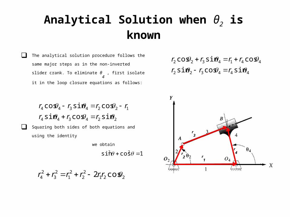
Analytical Solution when θ2 is known
The analytical solution procedure follows the same major steps as
in the non-inverted slider crank. To eliminate θ4
, first isolate it in
the loop closure equations as follows:
Squaring both sides of both equations and using the identity
we obtain
1cossin 22
22122
21
23
24 cos2 rrrrrr
r3
r2 r
1
r4
224344
1224344
sincossin
cossincos
rrr
rrrr
444322
4414322
sincossin
cossincos
rrr
rrrr
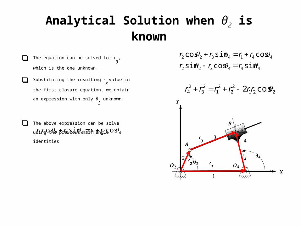
Analytical Solution when θ2 is known
The equation can be solved for r3
, which is the one
unknown.
Substituting the resulting r3
value in the first closure
equation, we obtain an expression with only θ3
unknown
The above expression can be solve using the previous
half angle identities
22122
21
23
24 cos2 rrrrrr
r3
r2 r
1
r4
444322
4414322
sincossin
cossincos
rrr
rrrr
4414322 cossincos rrrr
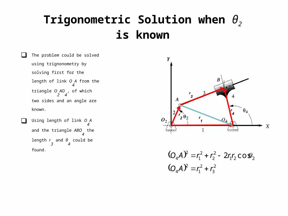
Trigonometric Solution when θ2 is known
The problem could be solved using
trignonometry by solving first for the
length of link O4
A from the triangle
O2
AO4
, of which two sides and an angle
are known.
Using length of link O4
A and the
triangle ABO4
the length r3
and θ4
could be found.
r3
r2 r
1
r4
2
321
24
22122
21
24 cos2
rrAO
rrrrAO
Analytical Solution when θ2 is known
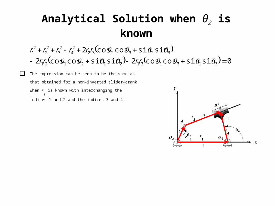
The expression can be seen to be the same as that obtained for a
non-inverted slider-crank when r1
is known with interchanging the
indices 1 and 2 and the indices 3 and 4.
r3
r2 r
1
r4
0sinsincoscos2sinsincoscos2
sinsincoscos2
313131212121
32323224
23
22
21
rrrr
rrrrrr
TRANSMISSION ANGLES
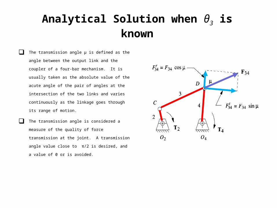
Analytical Solution when θ3 is known
The transmission angle μ is defined as the angle between the
output link and the coupler of a four-bar mechanism. It is
usually taken as the absolute value of the acute angle of the
pair of angles at the intersection of the two links and varies
continuously as the linkage goes through its range of motion.
The transmission angle is considered a measure of the quality
of force transmission at the joint. A transmission angle value
close to π/2 is desired, and a value of 0 or is avoided.

![Fluid Mechanics - An-Najah National Universityvideos.najah.edu/sites/default/files/3--1.pdf · [3] Fall –2010 –Fluid Mechanics Dr. Mohammad N. Almasri [3-1] Fluid Statics Pressure](https://img.pdfslide.us/doc/110x75/5a8724087f8b9a14748d4e3e/fluid-mechanics-an-najah-national-3-fall-2010-fluid-mechanics-dr-mohammad.jpg)


![Fluid Mechanics - An-Najah Videos · [3] Fall –2010 –Fluid Mechanics Dr. Mohammad N. Almasri [3-1] Fluid Statics Fluid Pressure Fluid pressure is the normal force exerted by the](https://img.pdfslide.us/doc/110x75/5adc4efd7f8b9a8b6d8b62a3/fluid-mechanics-an-najah-videos-3-fall-2010-fluid-mechanics-dr-mohammad.jpg)