Al A I '11 :3l MECHANICS OF ICE JAM FORMATION IN RIV[RS(Ul COl|R fGIONS RFSEARCH AND ENGINEERINi LAB HANOVER NHlN I ACKIRMANN [I AL DEC 83 CRR81 83 31

II( I ', hhh hhh) Ih, FA I

I~lllllll4

Lm"

V IA

SI

It I1 1,

1.2 I 'lK 11.6

MICROCOPY RESOLUTION TEST CH4ART

NATIONAL BUREAU OF STAN4POS - 63 -A

ADA1 38371 ZI

US Army CorpsREPORT383831.FEB2 - of Engineers

Cold RgosRsacEngineering Laboratory

Stib~o ju lift

Mechanics of ice ja0omaininrvr

-.9

For conversion of SI metric units to U.S./Britishcustomary units of measurement consult ASTMStandard E380, Metric Practice Guide, publishedby the American Society for Testing and Materi-als, 1916 Race St., Philadelphia, Pa. 19103.

Cover: Simulating river ice transport withsuspended plastic disks In an airtable chute.

I

,iI! I

CRREL Report 83-31December 1983

Mechanics of ice jam formation in rivers

Norbert L. Ackermann and Hung Tao Shen

PI'

1.

i i

UnclassifiedSECURITY CLASSIFICATION Of THIS PAGE ("o/an Data Entsrod9

PAGE READ INSTRUCTIONSREPORT DOCUMENTATION PBEFORE COMPLETING FORMI. REPORT NUMBER 2. GOVT ACCESSION NO. 3. RECIPIENT'S CATALOG NUMBER

CRREL Report 83-31 l b 4 if ?a *7 _

4. TITLE (aidSubtitle) S. TYPE OF REPORT & PERIOD COVERED

MECHANICS OF ICE JAM FORMATION IN RIVERS

6. PERFORMING ORG. REPORT NUMBER

7. AUTHOR(q) 8. CONTRACT OR GRANT NUMBER(*)

Norbert L. Ackermann and Hung Tao Shen

e. PERFORMING ORGANIZATION NAME AND ADDRESS 10. PROGRAM ELEMENT, PROJECT, TASK

AREA & WORK UNIT NUMBERSClarkson College of Technology CWIS 31750Potsdam, New York

11. CONTROLLING OFFICE NAME AND ADDRESS 12. REPORT DATE

Office of the Chief of Engineers December 1983Washington, D.C. 20314 Is. NUMBER OF PAGES

2114. MONITORING AGENCY NAME & ADDRESS(If difterent from Controllig Office) IS. SECURITY CLASS. (of this report)

U.S. Army Cold Regions Research and Engineering LaboratoryHanover, New Hampshire 03755 Unclassified

IS&. OECL ASSI FICATION/ DOWN GRADINGSCHEDULE

I*. DISTRIBuTION STATEMENT (.of dift Repori)

Approved for public release; distribution unlimited.

17. DISTRIBUTION STATEMENT (of the abstract entered In Block 20, It different fom Report)

Is. SUPPLEMENTARY NOTES

19. KEY WORDS (Conth,,,e # overs* aide it necessar d Identity by block number)Hydraulics Mathematical modelIce RiversIce bridge Surface ice jamIce jam

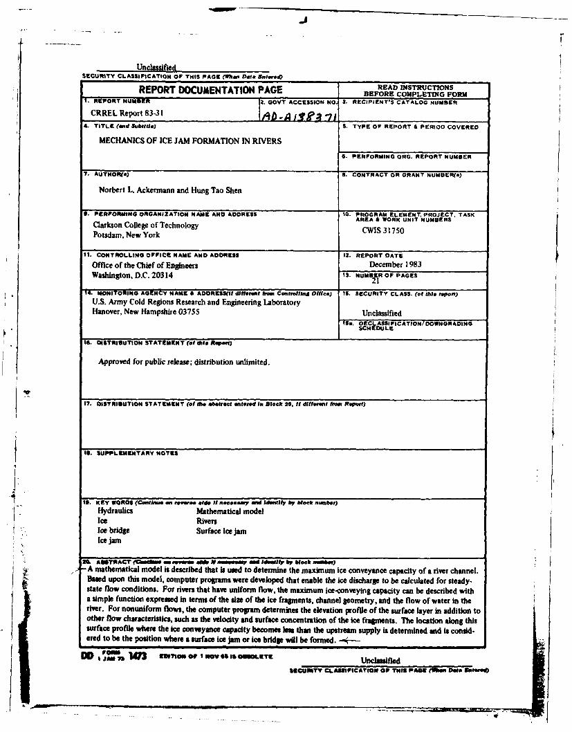
ft ATmACr (Cm" = mve rsora N amm w my fdelfy by blek tnmber)A mathematical model is described that is used to determine the maximum ice conveyance capacity of a river channel.

anted upon this model, computer programs were developed that enable the ice discharge to be calculated for steady-state flow conditions. For rivers that have uniform flow, the maximum ice-conveying capacity can be described witha simple function expressed in terms of the size of the ice fragments, channel geometry, and the flow of water in theriver. For nonuniform flows, the computer program determines the elevation profile of the surface layer in addition toother flow characteristics, such as the velocity and surface concentration of the ice fragments. The location along thissurface profile where the ice conveyance capacity becomes less than the upstream supply is determined and is consid-ered to be the position where a surface ice jam or ice bridpe will be formed. ---

DD,~, 343 M'"lon or IOSS mov to w aeI UnclassifiedSIECUIUN1 CLAM5FICATIO11 O0 TWOS PAOl (1010 D0e re

' -

PREFACE

This report was prepared by Norbert L. Ackermann and Hung Tao Shen of Clarkson Collegeof Technology, Potsdam, New York. Funding for this research was provided by Civil WorksProgram, Ice Engineering. CWIS 31750, Prediction of Ice Formation.

The authors have benefited greatly from discussions with G.E. Frankenstein, G.D. Ashton andD.J. Calkins regarding the mechanics of the formation of river jams.

I3'

ii

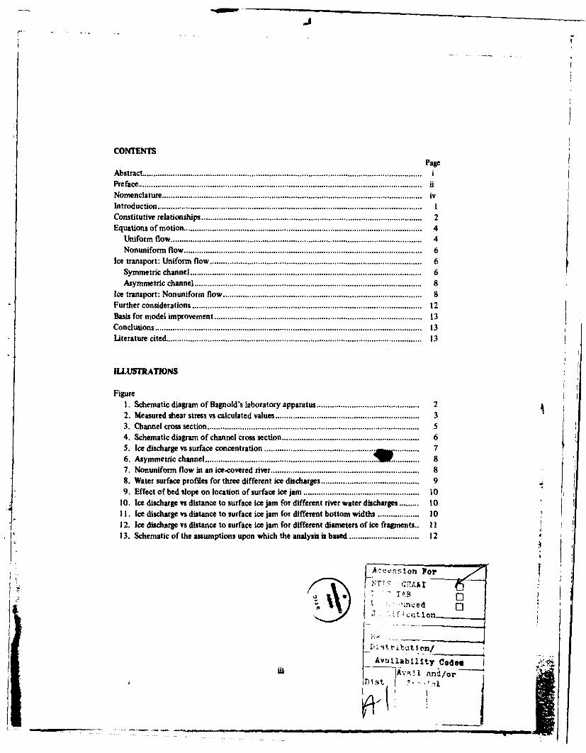
CONTENTSPage

Abstract.......................................................................................Preface ......................................................................................... uNomenclature................................................................................... ivIntroduction..................................................................................... IConstitutive relationships ........................................................................ 2Equations of motion.............................................................................. 4

Uniform flow ................................................................................. 4Nonuniform flow.............................................................................. 6

Ice transport: Uniform flow...................................................................... 6Symmetric channel............................................................................ 6Asymmetric channel........................................................................... 8

Ice transport: Nonuniform flow ................................................................. 8Further considerations........................................................................... 12Basis for model improvement.................................................................... 13Conclusions..................................................................................... 13Li4terature cited .................................................................................. 13

ILLUSTRATINS

Figure

I . Schematic diagram of Bagnold's laboratory apparatus................................... 22. Measured shear stress vs calculated values ................................................ 33. Channel cross section...................................................................... 54. Schematic diagram of channel cross section.............................................. 6S. Ice discharge vs; surface concentration ........................................ 76. Asymmetric channel ............................................................ 87. Nonuniform flow in an ice-covered river ................................................. 88. Water surface profiles for three different ice discharges ................................. 99. Effect of bed slope on location of surface ice jam....................................... 10

10. Ice discharge vs distance to surface ice jam for different river water discharges....... 10]IL Ice discharge vs distance to surface ice jam for different bottom widths.............. 1012. Ice discharge vs distance to surface ice jam for different diameters of ice fragments I I13. Schematic of the assumptions upon which the analysis is based ................... 12

Ac',,sslon For

'.nce4

D: ctthtlon

Avulalilty Codes

IlllAv,.l flna/or-

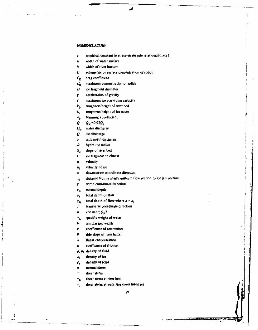
NOMENCLATURE

a empirical constant in stress-strain rate relationship, eq I

B width of water surface

b width of river bottom

C volumetric or surface concentration of solids

CD drag coefficient

C0 maximum concentration of solids

D ice fragment diameter

g acceleration of gravity

I maximum ice-conveying capacity

kb roughness height of river bed

ki roughness height of ice cover

nb Manning's coefficient

Q Qw +0.92Q i

Qw water discharge

Qj ice discharge

q unit width discharge

R hydraulic radiusSo slope of river bed

t ice fragment thickness

u velocityui velocity of ice

x downstream coordinate direction

x i distance from a nearly uniform flow section to ice jam section

y depth coordinate directionYn normal depth

Yt total depth of flow

Ytj total depth of flow where x = xjz transverse coordinate direction

a constant; Qi!!

ow specific weight of water

6 annular gap width

e coefficient of restitution

0 side slope of river bank

A linear concentration

p coefficient of friction

p, pf density of fluidPi density of ice

p, density of solid

a normal stress

shear stress

7b shear stress at river bed

r' shear stress at water/ice cover interface

iv

,.,I

MECHANICS OF ICE JAMFORMATION IN RIVERS

Norbert L. Ackermann and Hung Tao Shen

INTRODUCTION

The principles that govern the motion of ice fragments on the surface of a river are of interest

because of their possible influence on the formation of a river's surface ice cover. When floating inisolation, an ice fragment moves at approximately the local surface velocity of the river or stream.However, if ice fragments occur in sufficient concentration, they collide with one another as wellas with the river banks, reducing their downstream velocity. The mutual interference created byadjacent ice fragments can significantly reduce a river's ice.carrying capacity. The extent of thisinterference depends upon the size distribution and physical characteristics of the ice fragments,their number density, and their mean velocity, as well as the boundary conditions formed by theriver banks.

This report presents an analysis of the stresses produced by the collisional transfer of momentumbetween adjacent ice fragments on a river's surface and describes how stresses influence a river's icetransporting capacity. The maximum ice.conveying capacity of a river can be determined using thetheoretical relationships developed in this report. If the upstream supply of ice particles exceedsthe maximum value, a rapid increase in the concentration of the surface layer develops and a sta-tionary cover starts to form.

During a river's prefreeze-up period, ice pans commonly form on the river surface and are trans-ported downstream with the river flow. These ice pans may grow in size and occur in sufficient

abundance to create a surface ice jam across the river or stream. This surface restriction or barriercauses the upstream progression of an ice cover, since the incoming ice supply cannot be transported

farther downstream. Such a surface ice jam or bridge also creates a potential location for a river ice

jam in the spring if ice fragments created upstream by spring break-up are arrested by this surfacebarrier.

It is believed that the motion of the surface layer created by the ice pans in the fall, as well asJfragmented ice elements in the stream following the spring break-up, can be described by the analy-

s presented in this report.

Aim -

J

CONSTITUTIVE RELATIONSHIPS

When ice fragments are transported along the surface of a river, the mixture of ice and water thatforms the surface layer can be considered as a material or continuum with its own distinctive mate-

rial properties. At rest, this surface layer forms a rigid boundary that is subject to stresses identicalto those that are produced at the river banks and bottom. Stresses within the rigid ice layer are thenof interest for determining ice thickening processes, the development of ice pressure ridges, or the

conditions for incipient break-up.Before a stationary, rigid ice cover is formed, the surface layer is formed from a mixture of ice

fragments, water, and slush that is transported downstream by gravity. The stresses generated within

this moving surface layer have a significant influence upon the rate with which the mixture is trans.

ported downstream and, ultimately, upon the conditions required for the formation of a rigid icecover.

If the stresses within the surface layer result from the collisional transfer of momentum between

adjacent particles, the flow of this layer is considered to be inertia-dominated. When a river is at itsmaximum ice-transporting capacity, the velocities of the ice fragments in the surface layer are of the

same order of magnitude as the average water velocities in the river. For these conditions, therefore,the assumption that the stresses within the surface layer are inertia-dominated appears to be reason-able. Although experimental information describing the stresses within a rapidly sheared mixture ofice fragments and water is not available, there are data available on the constitutive (stress-strainrate) relationships of other cohesionless granular solids that can be modified to provide information

about the stress state that would exist in the surface layer of a river covered with rapidly flowing icefragments.

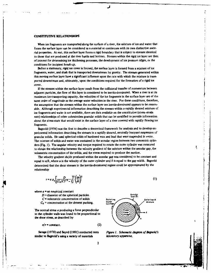
Bagnold (1954) was the first to describe a theoretical framework for analysis and to develop ex-perimental information describing the stresses in a rapidly sheared, neutrally buoyant suspension of

granular solids. He used spherical solids of hardened wax and lead that were suspended in weter.

The mixture of solids and water was contained in the annular region between two concentric cylin-

ders (Fig. 1). The angular velocity and torque required to rotate the outer cylinder was measuredto obtain the relationship between the velocity gradient of the mixture within the annular gap, the

volumetric concentration of the solids, and the stress required to produce the motion.

The velocity gradient du/dz produced within the annular gap was considered to be constant and

equal to u/8, where u is the velocity of the outer cylinder and 6 is equal to the gap width. Bagnold

determined that the shear stresses in the inertia-dominated regime could be approximated by the

relationship

7 a ,, 01 C)(1

where a = an empirical constantD diameter of the spherical particles Ap u)I

C = volumetric concentration of solids Rotting Solid-liquid

Co = concentration at the densest packing. Outer MijtureCylinder

The normal stress a producing a force perpendicular Ftzto the cylinder walls was found to be proportional to Cylinde

the shear stress, as described by U

O/r constant. (2)

Savage (1978) and Sayed (1981) conducted tests Figure 1. Schenmtic diagrm of Basold'ssimilar to BDaold's using a variety of materials laboratory apparatus.

2

I!

- -.-------------.---

4.I

create different solid-liquid mixtures, but the mixture for which experimental data was availablethat most closely represented the ice fragments and water found on a river surface is the mixture ofhard wax spheres in water that was first studied by Bagnold (1954).

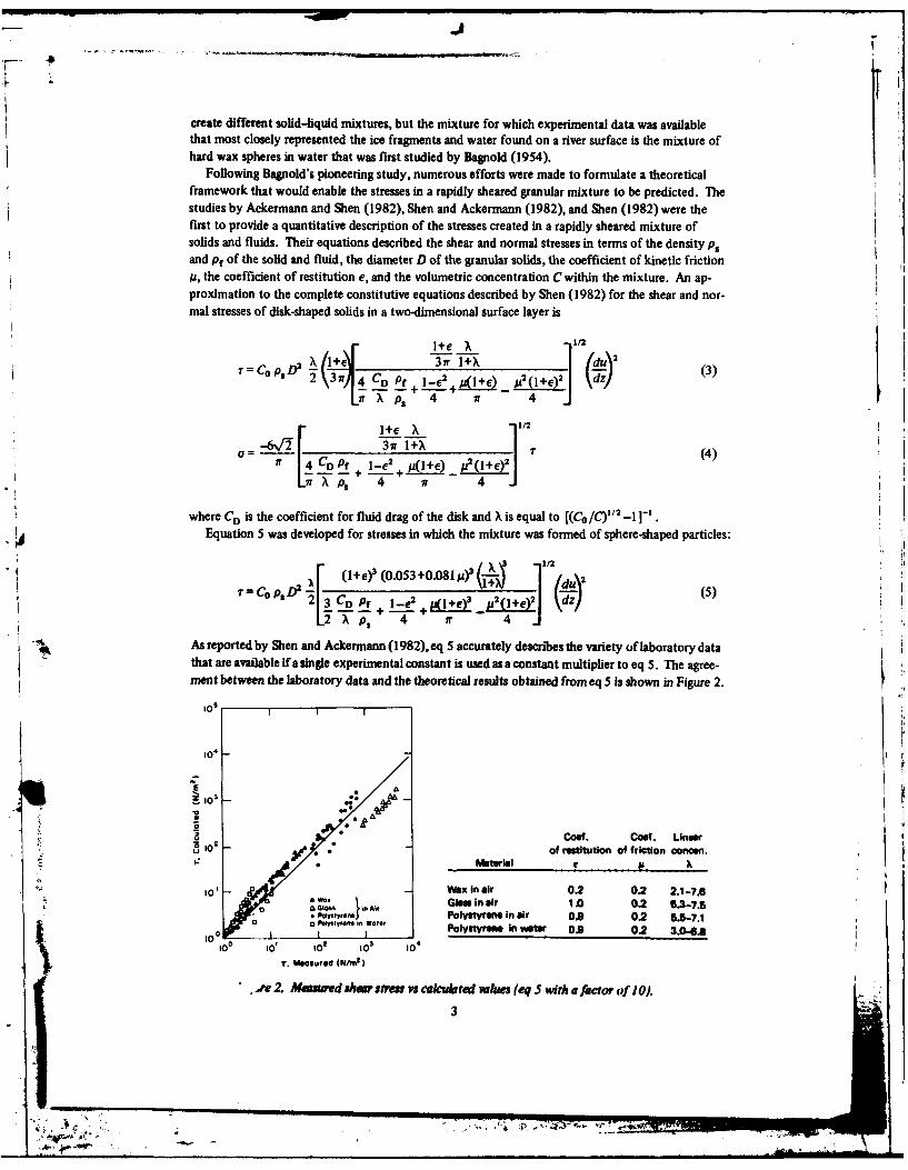
Following Bagnold's pioneering study, numerous efforts were made to formulate a theoreticalframework that would enable the stresses in a rapidly sheared granular mixture to be predicted. Thestudies by Ackermann and Shen (1982), Shen and Ackermann (1982), and Shen (1982) were thefirst to provide a quantitative description of the stresses created in a rapidly sheared mixture ofsolids and fluids. Their equations described the shear and normal stresses in terms of the density p.and pf of the solid and fluid, the diameter D of the granular solids, the coefficient of kinetic frictionj, the coefficient of restitution e, and the volumetric concentration C within the mixture. An ap-proximation to the complete constitutive equations described by Shen (1982) for the shear and nor-mal stresses of disk-shaped solids in a two-dimensional surface layer is

l+e X 112

33 7Aw3 (2SCD l-e2 p(l+e)2 ( (4)iX p. 4 Vr 4

where CD is the ~ rcoefficient for fluid drag of the disk and X is equal to [(C0o/C)"/2 -1J ]-.Equation 5 was developed for stresses in which the mixture was formed of sphere-shaped particles:

.r (~l+ C'5+'8p(--6F 31 c.If: +X~ (4)

CPf +-2 u1e ~ Z 5X S 4 7 4

" qtAs reported by Shen and Ackermann (1982), eq 5 accurately describes the variety of laboratory datathat are available ifa single experimental constant is usedasaconstant multiplier to eq . The agree-ment between the labotory data and the theoretical results obtained from eqS is shown in Figure 2.

I102

!•a 3

oz 9.0z _ -of restitution of friction concert.

0 Wax In air .2 0.2 2.1-76

S1. G&e in air 1.0 0.2 6.(-7.5,~ le Polystyrene in air 0 .9 0.2 5 -7.1

iO I PoI. I~WO Polystyrene in wes 0.9 0.2 3.06100 3 |01 Pf 104

r, Measured (N/rn')

t e 2. Mumued ahw r es vs calculated whies (eq s wth a factor of 10).

P - - + 4

The data presented consist of all published data presently available and include tests in which thesolids were either of hardened wax, polystyrene, or glass and the fluid was either water or air. Lab-oratory data were not available, however, with which to determine the validity of eq 3 describingthe shear stresses in a surface layer of disk-shaped solids. The ratio of eqs 3 and 5 was therefore usedas a multiplying factor to convert Bagnold's experimental data for rapidly sheared sphere-shapedsolids to an equation appropriate for disk-shaped solids, such as ice fragments on the surface of astream. Chiou (1982) describes in detail how eqs 3 and 5 and other independent methods were usedto modify Bagnold's experimental results to determine the constitutive relationships for rapidlysheared disk-shaped solids in a two-dimensional layer. Each of the methods used to modify eq I torepresent the motion of disk-shaped solids produced approximately similar results. Chiou deter-mined that the equation that best described the shear stress in a surface layer of ice fragments is

r = 0.021 pi X(l + X) D2 (du/dz) 2 (6)

where X = [(0.91/C),12 - 1

pi = density of iceD = ice fragment diameter

du/dz = velocity gradientof the surface ice layer.

EQUATIONS OF MOTION

Uniform flowThe motion of the surface ice layer in a river is produced by the downstream component of the

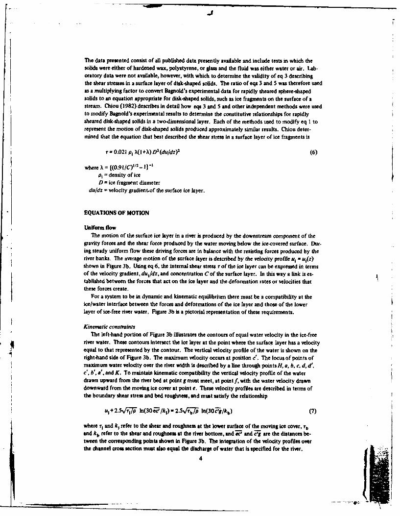
gravity forces and the shear force produced by the water moving below the ice-covered surface. Dur.ing steady uniform flow these driving forces are in balance with the resisting forces produced by theriver banks. The average motion of the surface layer is described by the velocity profile ui = u1(z)shown in Figure 3b. Using eq 6, the internal shear stress r of the ice layer can be expressed in termsof the velocity gradient, dui/dz, and concentration C of the surface layer. In this way a link is es-tablished between the forces that act on the ice layer and the deformation rates or velocities thatthese forces create.

For a system to be in dynamic and kinematic equilibrium there must be a compatibility at theice/water interface between the forces and deformations of the ice layer and those of the lowerlayer of ice-free river water. Figure 3b is a pictorial representation of these requirements.

Kinematic constraintsThe left-hand portion of Figure 3b illustrates the contours of equal water velocity in the ice-free

ariver water. These contours intersect the ice layer at the point where the surface layer has a velocityequal to that represented by the contour. The vertical velocity proffle of the water is shown on theright-hand side of Figure 3b. The maximum velocity occurs at position c'. The locus of points ofmaximum water velocity over the river width is described by a line through points H, a, b, c, d, d',c', b', a', and K. To maintain kinematic compatibility the vertical velocity profile of the waterdrawn upward from the river bed at point g must meet, at point f, with the water velocity drawndownward from the moving ice cover at point e. These velocity profiles are described in terms ofthe boundary shear stress and bed roughness, and must satisfy the relationship

u, + 2.5vr'T7 ln(3Oe'/k 1 )- 2.SV~7~ ln(30Og-/kb) (7)

where rj and k, refer to the shear and roughness at the lower surface of the moving ice cover, rband kb refer to the shear and roughness at the river bottom, and W; and crg are the distances be-tween the corresponding points shown in Figure 3b. The integration of the velocity profiles overthe channel cross section must also equal the discharge of water that is specified for the river.

4

2 ~P

Ii

a. Schematization for numerical solution.

Hz

Velocity Profile X

of Ice Layer orUi Ui (Z) C..e. C ef._ X

Equal VelocityContours

b. Velocity contours and velocity profile of surface ice layer.

Figure 3. Channel cross section.

Dynamic equilibriumThe shear stress r within the ice layer and the boundary stresses i, and Tb can all be determined

i from force balances on free-body diagrams of elements within the flow system. If r, Ti, and Tb areI to be the only stresses involved in the free-body analysis, the selection of the free bodies must de-

pend upon the shape of the velocity contours shown in Figure 3b. Since the line through points.1 H, a, b, c, d, d', c', b', a', and K represents a locus of points of maximum velocity, it can be as.sumed that this is also a line along which the longitudinal shear stress is zero. This can be furtherillustrated by considering the vertical velocity profile shown on the right-hand side of Figure 3b.Since dudy at pointfon the vertical velocity proftle is zero, the shear sur e is also equal to zero,

since fluid stresses are proportional to some power of the velocity gradient. For a river with uni-form flow and no ice cover, the total area HIJII multiplied by the bed slope and specific weightof water would equal the total resistance force per unit length of river exerted by the bed shear .For an ice-covered channel, the saded area on the righthand side of Figure 3b multiplied by the

bed slope S0 and specific weight 'yw of water therefore represents the force per unit of river lengthacting on the ie-overed surface. In steady uniform flow, the boundary stresses can be detcribedby the relationships

H, a , ,d d, c', bs, a' an( ersnsalcso onso aiu eoiy tcnb s

S(Tb). "*v.So i (9)

Si

... ........ ................ line al n wh c the... . . . ... .... l n iti na ....... stes isz r .T i c n b u t e

,,J

where (Ti). and (Tb)s refer to the boundary stresses at locations e and g, respectively. The equa-tion for the stress T within the ice cover KK'JJL is obtained from a force balance on the free body(Fig. 3b). This force balance includes the downstream component of the weight of the ice fragmentsand water contained in the surface layer as well as the shear forces on the underside of the ice layerrepresented by the shaded area LMb'aKL.

These conditions for dynamic equilibrium and kinematic compatibility enable sufficient equa-tions to be written to determine the velocity and volume rate of flow of the ice in the surface lay-er. The formulation of these equations and their method of solution are described by Ackermann(1979), Free (1979), and Chiou (1982). The solution procedure involves discretizing the channelinto P strips or volume elements, as shown in Figure 3 a. The equations of motion were written forthe water and ice portions of each of the volume elements. These equations were then solved nu-merically.

Nonuniform flowNumerous complications are introduced by considering conditions where the river's depth

changes in the direction of flow. The stresses T1 and Tb can no longer be described by eq 8 and 9,since there is then a variation in the momentum flux in the stream direction. Since none of thechannel boundaries then have parallel surfaces, the geometric complexities involved in discretizingthe channel into subelements greatly complicate the analysis. For nonuniform flow conditionsthere are also nonzero values of the transverse mass and momentum flux between each of the Psubelements. The development of the equations of motion considering these nonuniform effects

is described by Chiou (1982).

ICE TRANSPORT: UNIFORM FLOW

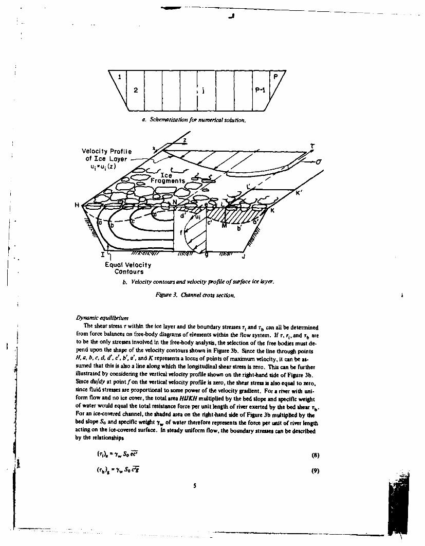
Synmetric channelThe ice-transporting capacity of the river shown in Figure 4 is to be determined when the flow

conditions are steady and uniform. Conditions of uniform flow represent an idealized situation inwhich the depth of flow as well as all other flow conditions remain constant along the length ofthe river. The channel shown in Figure 4 is symmetric about its centerline, which further simpli-fies the analysis.

If the number density of the ice fragments on the river surface is sufficiently low, there will befew collisions between the ice particles and the river banks. The gravity component of the ice/water system in the stream direction can then be assumed to be balanced entirely by the shearstresses t b between the water and the river banks and bottom. In such a situation, the normaldepth y, can be approximated from the Manning equation expressed in the following form:

I" bQ 1 31 (10)

where R(y,) is the hydraulic radius ofthe channel cross section that can beexpressed in terms of the normal depth B

Y., Yb is Manning's coefficient for theriver bed, and Q is equal to Q,+0.92Q,, where 0.92 Qj represen ts the vol-ume of ice transformed to its equiv-

alent volume of water. At low sur-face concentrations, the volume flow b

rate of the ice can be expressed as Fige 4. Schenmtic digram of channel cross section.

6

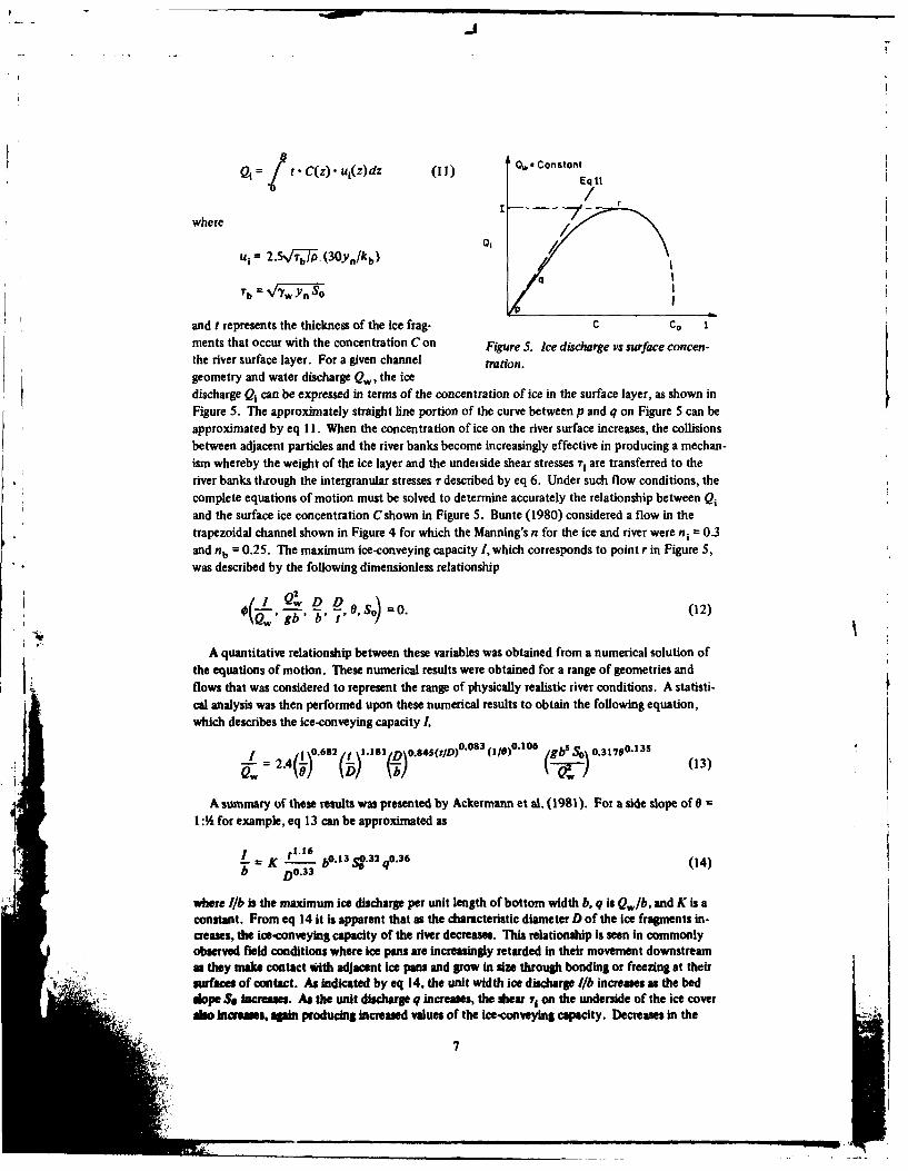
Qi t -t C(z) - u(z) dz (1.-Ow Constont

Eq It

whereci /

u,= 2.Sv'IT.(30y,/kb)= I

tb ,V'VW Y. So

and t represents the thickness of the ice frag- C CO I-ments that occur with the concentration Con Figure 5. Ice discharge vs surface concen-the river surface layer. For a given channel tration.geometry and water discharge Qw, the ice

discharge Qi can be expressed in terms of the concentration of ice in the surface layer, as shown inFigure 5. The approximately straight line portion of the curve between p and q on Figure 5 can beapproximated by eq 11. When the concentration of ice on the river surface increases, the collisionsbetween adjacent particles and the river banks become increasingly effective in producing a mechan-ism whereby the weight of the ice layer and the unde, side shear stresses Ti are transferred to theriver banks through the intergranular stresses r described by eq 6. Under such flow conditions, thecomplete equations of motion must be solved to determine accurately the relationship between Qiand the surface ice concentration C shown in Figure 5. Bunte (1980) considered a flow in thetrapezoidal channel shown in Figure 4 for which the Manning's n for the ice and river were n i = 0.3and nb = 0.25. The maximum ice-conveying capacity 1, which corresponds to point r in Figure 5,was described by the following dimensionless relationship

(w Qiw D D O , =. (12)Q' gb' b' t i

A quantitative relationship between these variables was obtained from a numerical solution ofthe equations of motion. These numerical results were obtained for a range of geometries andflows that was considered to represent the range of physically realistic river conditions. A statisti-cal analysis was then performed upon these numerical results to obtain the following equation,which describes the ice-conveying capacity I,

1 jl 0,I , (O.S45(t)D)0 03(1/0).106 gbSSo 0.3170 -13 5

-= 2" " t ) (-r) (13)

A summary of these results was presented by Ackermann et al. (1981). For a side slope of 9 =

1: for example, eq 13 can be approximated as

I-I

/ K ! bp.'13 S .32 q 0 .36 (14)T D 0.33

where I/b is the maximum ice discharge per unit length of bottom width b, q is Qw/b, and K is aconstant. From eq 14 it is apparent that as the characteristic diameter D of the ice fragments in-creases, the ice-conveying capacity of the river decreases. This relationship is seen in commonlyobserved field conditions where ice pans are increasingly retarded in their movement downstreamas they make contact *ith adjacent ice pans and grow in size through bonding or freezing at theirsurfaces of contact. As indicated by eq 14, the unit width ice discharge Ib increases as the beddope S Increases. As the unit discharge q increases, the shear Ti on the underside of the ice coveralso increases, spin producing increased values of the ice-conveying capacity. Decreases in the

7

unit discharge Ib are produced by a decrease in the river's base width b. This decrease occurssince, for the same unit discharge, a reduction in the channel width b produces an increase in thevelocity gradient du1/dz, which, as shown in eq 6, increases the intergranular stress within the ice/water mixture in the surface layer.

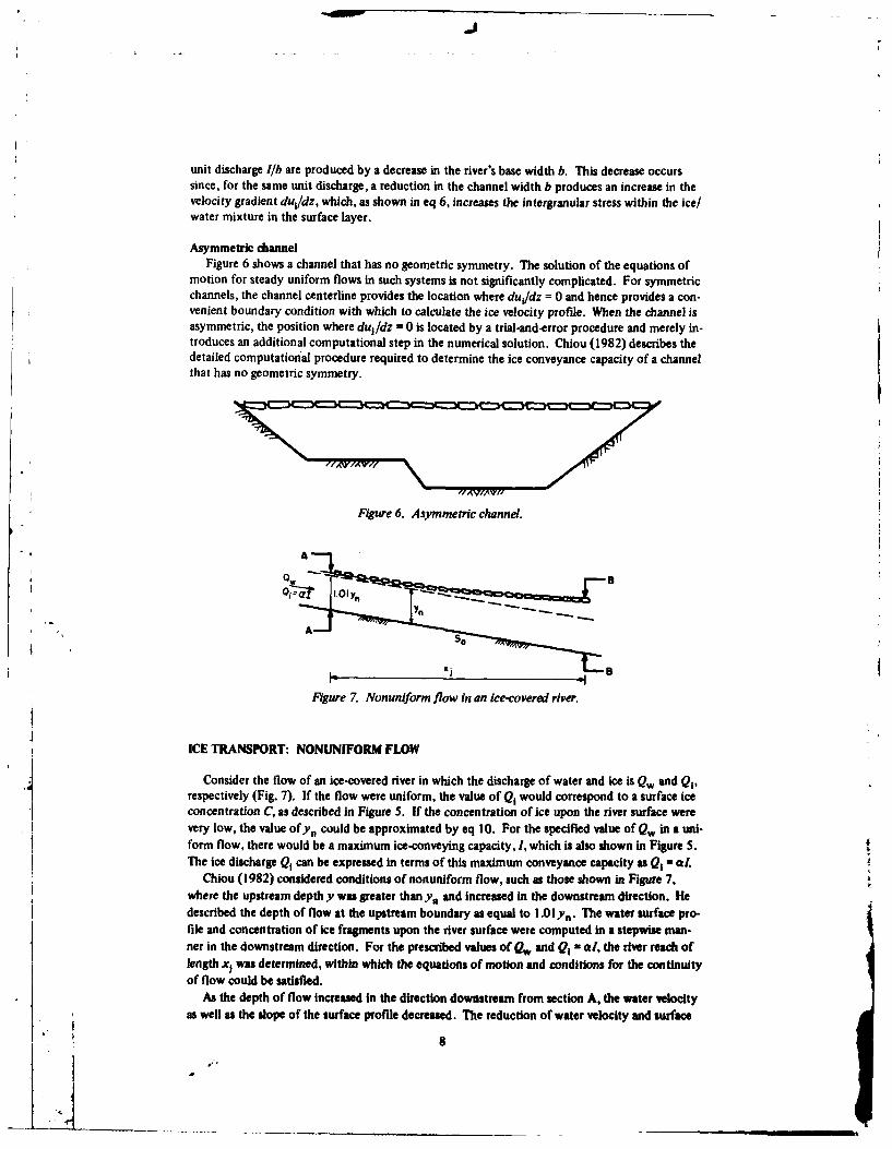
Asymmetric channelFigure 6 shows a channel that has no geometric symmetry. The solution of the equations of

motion for steady uniform flows in such systems is not significantly complicated. For symmetricchannels, the channel centerline provides the location where dujdz = 0 and hence provides a con-venient boundary condition with which to calculate the ice velocity profile. When the channel isasymmetric, the position where dui/dz = 0 is located by a trial-and-error procedure and merely in-troduces an additional computational step in the numerical solution. Chiou (1982) describes thedetailed computational procedure required to determine the ice conveyance capacity of a channelthat has no geometric symmetry.

Figure 6. Asymmetric channel.

A

i . B

Figure 7. Nonuniform flow in an ice-covered river.

ICE TRANSPORT: NONUNIFORM FLOW

Consider the flow of an ice-covered river in which the discharge of water and ice is Qw and Q,respectively (Fig. 7). If the flow were uniform, the value of Q, would correspond to a surface iceconcentration C, as described in Figure 5. If the concentration of ice upon the river surface werevery low, the value of y, could be approximated by eq 10. For the specified value of Qw in a uni-form flow, there would be a maximum ice-conveying capacity, 1, which is also shown in Figure 5. 4The ice discharge Q can be expressed in terms of this maximum conveyance capacity as Q,= 1. .

Chiou (1982) considered conditions of nonuniform flow, such as those shown in Figure 7,where the upstream depth y was greater than y, and increased in the downstream direction. Hedescribed the depth of flow at the upstream boundary as equal to 1.01 y. The water surface pro-file and concentration of ice fragments upon the river surface were computed in a stepwise man-ner in the downstream direction. For the prescribed values of Qw and Q, = aI, the river reach oflength x1 was determined, within which the equations of motion and conditions for the continuityof flow could be satisfied.

As the depth of flow increased in the direction downstream from section A, the water velocityas well as the slope of the surface profile decreased. The reduction of water velocity and surface

8

slope correspondingly reduced the driving force on the ice layer, thereby producing an increase inthe concentration C of the ice fragments on the surface and a reduction in their downstream velo-city ui. As long as the product of the surface concentration and the velocity of the ice particlescould provide for the transport of the specified upstream ice supply Q as shown by eq 15, steady-state flow conditions could be maintained and the equations of motion would be satisfied.

R

Q=al= tf vi(z,x) C(z,x)dz. (15)0

By traveling sufficiently far downstream, however, a location such as section B will eventuallybe reached where a set of values ui(z) and C(z) cannot be found that satisfy the equations of mo-tion. The volume rate of flow Qi established at the upstream boundary can therefore not be main-tained below that section, and unsteady-state conditions are created. The concentration of ice atsection B will increase with time, the ice fragments will be compressed by forces from the upstreamflow, and a solid ice cover will start to form. This situation creates the conditions required to initi-ate an ice jam or obstruction of the surface layer at location B.

Chiou (1982) simulated numerous flow situations by solving the equations of motion for non-uniform flows in a river with a trapezoidal cross section. He developed the digital computer pro-gram that was used to find the numerical solutions; it was restricted to nonuniform flows in sym-metric channels in which the depth increased in the downstream direction. Figures 8 through 12provide some of Chiou's (1982) results.

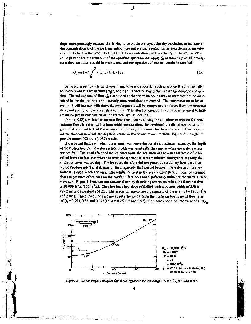
It was found that, even when the channel was conveying ice at its maximum capacity, the depthof flow described by the water surface profile was essentially the same as when the water surfacewas ice-free. The small effect of the ice cover upon the deviation of the water surface profle re-

suited from the fact that when the river transported ice at its maximum conveyance capacity theentire ice cover was moving. The ice cover therefore did not present a stationary boundary thatwould produce interfacial stresses of the magnitude that existed between the water and the riverbottom. Hence, when applying these results to rivers in the pre-freezeup period, it can be assumedthat the presence of ice pans on the river's surface does not significantly influence the water surfaceelevation. Figure 8 demonstrates this condition by describing conditions when the flow in a riveris 30,000 ft3 /s (850 m 3 Is). The river has a bed slope of 0.0001 with a bottom width of 250 ft(77.2 m) and side slopes of 2: 1. The maximum ice-conveying capacity of the river is I = 1950 ft 3 /S

(55.2 m3 ). Three conditions are given, with the ice entering the upstream boundary at flow ratesof Qi = 0251,0.51, and 0971 (i.e. ac 0.25,0.5 and 0.97). For these conditions the value of 10y n

00

a-0.25t~i

90-0.0001

20 01. 7 0- loftt=2 ftI _960 ft3 I

0 40 -120 10 Y 225ftfora-0.25 ad.5

O,ta.Ce (miles) 22.6 ft for a 0.97

Fiure 8. Water surfaee pro lies for three different ice dbehrges to -0.25, 0.5 and 0. 9 7).

9

.. . ...

C I OI

MEMO!

So. 0.000110.001 (1-1950 tt 3

/5)3895)

4-- -.

0C /" - . 0,00001

00 0w = 30,000 ft3 1s

2 (I2 It

D - 10 ft

0 10 20 30xl0 4

Dimensionless Length

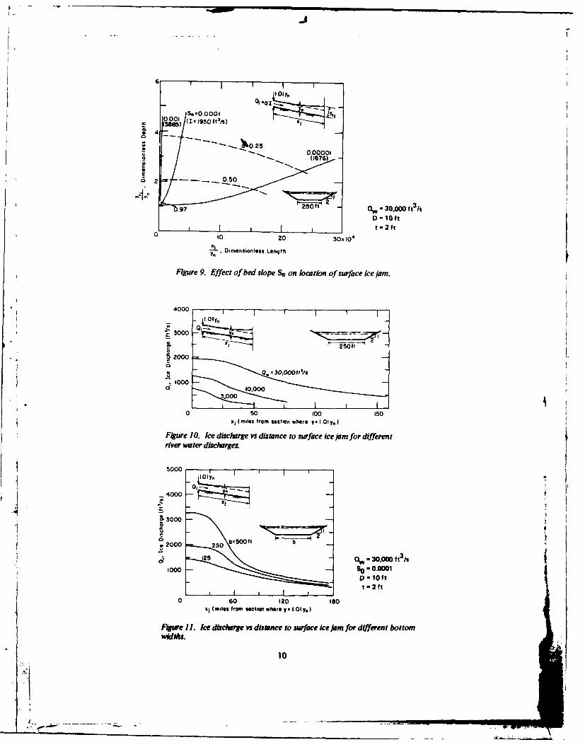
Figure 9. Effect of bed slope So on location of surface ice jam.

4000 I I I

-1i 3000

250f1

_2000

o 0. ; '30,,00tl's

-1000

3.000

00 so00 150

x, (miles from section where y- • ,0yn )

Figue 10. Ice discharge vs distance to surface ice jam for differentriver wter discharges.

50 0 0 1 s 1I

4000

93000

2000 2 50 0 f b

125 Q, 3.000 It /Z1000 SO -0.0001

D - 10ft

• I I+ I t =2 ft

0 60 120 ISOR, (miles from beciotf where y I.Oly,)

Figure 11. Ice discharge vs disnce to surface ice jam for d(fferent bottom"Widhs.

10

uha

_J

400CIlOly n

)C " " 250 ft -

O0,2- ft (1. 265 Wt/o)

- 0, -30000 t3/

So- o.OOlS60 120 ISO t - 2 ft

x, (miles from section where y-l.Oly,)

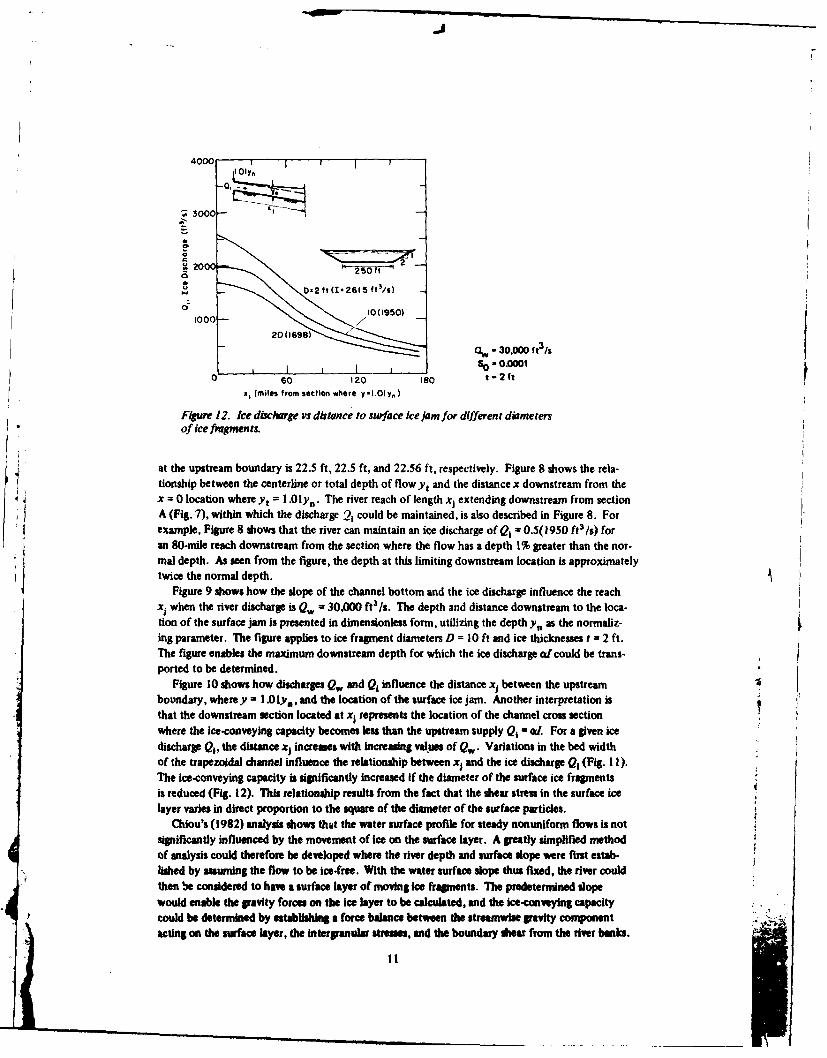
Figure 12. Ice discharge vs distance to surface ice jam for different diametersof ice fragments.

at the upstream boundary is 22.5 ft, 22.5 ft, and 22.56 ft, respectively. Figure 8 shows the rela-tionship between the centerline or total depth of flow Yt and the distance x downstream from thex = 0 location where Yt = 1.Oly,. The river reach of length xj extending downstream from sectionA (Fig. 7), within which the discharge 21 could be maintained, is also described in Figure 8. Forexample, Figure 8 shows that the river can maintain an ice discharge of Qi -0.5(l950 ft 3/s) foran 80-mile reach downstream from the section where the flow has a depth 1% greater than the nor-mal depth. As seen from the figure, the depth at this limiting downstream location is approximatelytwice the normal depth.

Figure 9 shows how the slope of the channel bottom and the ice discharge influence the reachxj when the river discharge is Qw - 30,000 ft3 /s. The depth and distance downstream to the loca-tion of the surface jam is presented in dimensionless form, utilizing the depth ya as the normaliz-ing parameter. The figure applies to ice fragment diameters D = 10 ft and ice thicknesses t = 2 ft.The figure enables the maximum downstream depth for which the ice discharge of could be trans-ported to be determined.

Figure 10 shows how discharges Qw and Q4 influence the distance xj between the upstreamboundary, where y - 1.0ly,, and the location of the surface ice jam. Another interpretation isthat the downstream section located at xj represents the location of the channel cross sectionwhere the ice-conveying capacity becomes less than the upstream supply Q, = ad. For a given icedischarge Qj, the distance xj increases with increasing values of Qw. Variations in the bed widthof the trapezoidal channel influence the relationship between x| and the ice discharge Qi (Fig. 1I).The ice-conveying capacity is significantly increased if the diameter of the surface ice fragmentsis reduced (Fig. 12). This relationship results from the fact that the shear stress in the surface icelayer varies in direct proportion to the square of the diameter of the surface particles.

Chiou's (1982) analysis shows that the water surface profile for steady nonuniform flows is notsignificantly influenced by the movement of ice on the surface layer. A greatly simplified methodof analysis could therefore be developed where the river depth and surface slope were first estab-lished by assuming the flow to be ice-free. With the water surface slope thus fixed, the river couldthen be considered to have a surface layer of moving ice frapnents. The predetermined slopewould enable the gravity forces on the ice layer to be calculated, and the ice-conveying capacitycould be determined by establishing a force balance between the streamwiue gravity componentacting on the surface layer, the intergranular stresm, and the boundary shear from the river banks.

11

In such an analysis. the shear stresses ri from the water would be ignored, and the results wouldthus underestimate the ice-conveying capacity. Such an analysis, however, would be very simpleto perform and would provide a reasonable approximate solution.

FURTHER CONSIDERATIONS

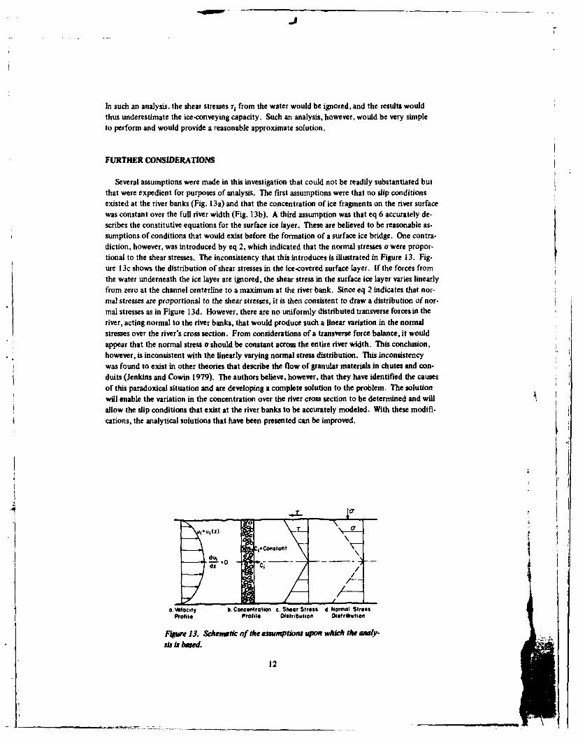
Several assumptions were made in this investigation that could not be readily substantiated butthat were expedient for purposes of analysis. The first assumptions were that no slip conditionsexisted at the river banks (Fig. 13a) and that the concentration of ice fragments on the river surfacewas constant over the full river width (Fig. 13b). A third assumption was that eq 6 accurately de-scribes the constitutive equations for the surface ice layer. These are believed to be reasonable as-sumptions of conditions that would exist before the formation of a surface ice bridge. One contra.diction, however, was introduced by eq 2, which indicated that the normal stresses o were propor-tional to the shear stresses. The inconsistency that this introduces is illustrated in Figure 13. Fig-ure 13c shows the distribution of shear stresses in the ice-covered surface layer. If the forces fromthe water underneath the ice layer are ignored, the shear stress in the surface ice layer varies linearlyfrom zero at the channel centerline to a maximum at the river bank. Since eq 2 indicates that nor-mal stresses are proportional to the shear stresses, it is then consistent to draw a distribution of nor-mal stresses as in Figure 13d. However, there are no uniformly distributed transverse forces in theriver, acting normal to the river banks, that would produce such a linear variation in the normalstresses over the river's cross section. From considerations of a transverse force balance, it wouldappear that the normal stress o should be constant across the entire river width. This conclusion,however, is inconsistent with the linearly varying normal stress distribution. This inconsistencywas found to exist in other theories that describe the flow of granular materials in chutes and con-duits (Jenkins and Cowin 1979). The authors believe, however, that they have identified the causesof this paradoxical situation and are developing a complete solution to the problem. The solutionwill enable the variation in the concentration over the river cross section to be determined and willallow the slip conditions that exist at the river banks to be accurately modeled. With these modifi-cations, the analytical solutions that have been presented can be improved.

~L11

d,* . conston 'n

/--

0. Velocity b. Conceritrotion c. Shear Stress d. Normal StressProfile Profile Oistribution Oistribution

Figure 13. &hewfic of the asumptions upon which the amly-s is tined.

12

BASIS FOR MODEL IMPROVEMENT

In Ackermann and Shen (1982), the authors developed a theory that describes the mechanismby which both normal and shear stresses are developed in a rapidly sheared granular material. Byincluding a single empirical constant, their theory has been shown to agree with experimental re-sults where granular mixtures have been sheared in the opening created between two closely spacedboundaries having a relative velocity y (Fig. I). Within such small gaps the velocity distribution isconsidered to be linear. If the granular flow occurs within boundaries that are not closely spaced,such as between two river banks, the mechanism for stress generation within the granular mixtureis believed to be more complicated than that previously reported by Ackermann and Shen (1982),who reported that Reynolds-type stresses were produced by the transfer of momentum betweencolliding particles. Unlike existing theories for describing the turbulence of homogeneous fluids,these Reynolds-type stresses could be accurately determined from theoretical considerations. Thelateral diffusion of the turbulent energy created by the collision of the ice fragments was ignored,however, when eq 6 was derived to describe the shear stresses in the mixture of ice and water on theriver's surface layer. To describe completely the stress state within the surface layer of a river, anenergy balance equation that includes the generation of turbulent energy within the mixture, itsdissipation into heat, and its lateral transfer must be considered. Only by introducing these modifi-cations will it be possible to obtain the complete solution to the problem of the transportation ofice on a river surface. The concentration of ice is not constant over the river's width, and the nor-mal stresses between the ice fragments and the river banks are an important quantity in the solution.The identification of these normal stresses will permit evaluation of the slip of ice fragments at theboundary.

By using the changes suggested above to modify the constitutive relationships and by includingthe simplifications that were made obvious from the work by Chiou (1982), a more accurate modelof the transportation of ice on a river surface can be developed. The authors are currently conduct-

ing laboratory tests in which disk-shaped solids are transported by gravity forces down a smoothand evenly inclined chute. Numerous holes on the chute surface provide a vertical air supply thatgreatly reduces the frictional forces between the disks and the surface of the chute. The correct

interpretation of the results from these tests is believed to depend upon obtaining an analyticalsolution to the problem described above, which considers the dispersion of turbulent energythrough the granular flow.

CONCLUSIONS

The maximum ice-conveying capacity of a river depends upon the amount of river water dis-charge, the channel geometry, the size of the ice fragments, the depth of flow, and the slope of thewater surface profile. A single equation has been found that describes the ice conveyance capacityof the channel when the flow in a river is uniform so that the depth of the flow remains constant.When the flow is nonuniform, however, the velocity and concentration of ice fragments upon theriver surface are obtained from a numerical solution of the equations of motion. If the volume

rate of the flow of ice supplied by the upstream reach of a river is specified, the depth of flow canbe determined at the point where the incoming supply exceeds the local ice-conveying capacity ofthe river. At such a location a surface ice jam is going to occur.

4 LITERATURE CITED

A&Anmn, N.L and H.H. Shen (1982) Stresses in rapidly sheared fluid-solid mixtures. Journalof Engineering Mechancs Division, ASCE, 10(EM 1): 95-113.

13

~.1

Ackermun, N.L., H.T. Shen and A.P. Free (1979) Mechanics of river ice jams. In Proceedings ofthe Third Engineering Mechanics Division Specialty Conference, Austin, Texas. American Societyof Civil Engineers, pp. 815-818.Ackermann, N.L, H.T. Shen and R.W. Ruges (1981) Transportation of ice in rivers. IARH-Inter-national Symposium on Ice, Quebec Cty, 1981. pp. 333-342.Banold, R.A. (1954) Experiments on gravity-free dispersion of large solid spheres in a Newtonianfluid under shear. Proceedings of the Royal Society. London, Ser. A, 225: 49-63.

aunte, D.A. (1980) Ice jam formation in trapezoidal channels. M.S. thesis, Clarkson College ofTechnology, Potsdam, New York.Chiou, K.F. (1982) Surface ice jams in rivers having nonuniform flow. Ph.D. dissertation, ClarksonCollege of Technology, Potsdam, New York.Free, A.P. (1979) Ice jam formation: A mathematical model. M.S. thesis, Clarkson College of Tech.nology, Potsdam, New York.Jenkins, J.T. and S.C. Cowin (1979) Theories for flow granular materials. In Symposium Volumeon Mechanics Applied to the Transport of Bulk Materials. Buffalo, New York: American Societyof Mechanical Engineers, pp. 79-89.Savage, S.B. (1978) Experiments of shear flows of cohesionless granular materials. In Proceedingsof the U.S.-Japan Seminar on Continuum Mechanical and Statistical Approaches in the Mechanicsof Granular Materials (S.C. Cowin and M. Satake, Eds.). Tokyo: Gakujutsu Bunken Fukyukai,pp. 241-254.Sayed, M. (198 1) Theoretical and experimental studies of the flow of cohesionless granular materials.Ph.D. dissertation, McGill University, Montreal, Part 1, 91 pp.Shen, H.H. (1982) Constitutive relationships for fluid-solid mixtures. Ph.D. dissertation, ClarksonCollege of Technology, Potsdam, New York.Sben, H.H. and N.L Ackermann (1982) Constitutive relationships of fluid-solid mixtures. Journalof Engineering Mechanics Division, ASCE, 108(EMS): 748-763.

14i1 ____

A facsimile catalog card in Library of Congress MARCformat is reproduced below.

Ackermann, Norbert L.Mechanics of ice jam formation in rivers / by Norbert

L. Ackermann and Hung Tao Shen. Hanover, N.H.: U.S.Cold Regions Research and Engineering Laboratory;Springfield, Va.: available from National TechnicalInformation Service, 1983.

iv, 21 p., illus.; 28 cm. ( CRREL Report 83-31. )Bibliography: p. 13.1. Hydraulics. 2. Ice. 3. Ice bridge. 4. Ice jam.

5. Mathematical model. 6. Rivers. 7. Surface icejam. I. United States. Army. Corps of Engineers.II. Cold Regions Research and Engineering Laboratory,Hanover, N.H. 03755. III. Series: CRREL Report83-31.