Mechanical)proper-es)of) nanosheets)by)AFM)

Mechanical proper-es of nanosheets by AFM

Suresh Kumar Journal club ,IMS group,21-‐02-‐2012

Outline

•  Why mechanical proper-es of 2D materials ? •  Introduc-on

•  Nano-‐ indenta-on Vs Peak Force QNM

•  Conclusions

Why mechanical proper-es of 2D materials are important ?

•  Macroscopic materials fracture are dominated by grain boundary defect and defects

•  Uncertainty in sample geometry , stress concentra-on and

distribu-on , structural defects for example Nano tubes

•  Applicability in flexible electronic applica-ons ex.MoS2 nanosheets •  Nanoelectromechanical systems(NEMS) –as resonators

•  2 D sheets geometry are precisely are defined and less sensi-ve to defects

Mechanical proper-es-‐Different AFM modes

Nano-‐Indenta-on Peak force-‐Quanta-ve

nanomechanical mapping

Harmonic force Microscopy

Nano-‐indenta-on

Ø  Hertz model-‐ Approach-‐retract cycle at the rate of 0.5 to 1 Hz (Very slow)

Ø  Every pixel in an image – force Vs piezo displacement curve is obtained Ø  Samples :Insulin fibrils, biological substrates ,polymeric materials

Peak Force QNM

Ø  Derjaguin–Muller–Toporov (DMT) in-‐built model -‐includes visco-‐elas-city and adhesion between -p and the surface

Ø  High-‐Resolu-on Mapping of Modulus and Adhesion

Ø  Direct Force Control Keeps Indenta-ons Small for higher Resolu-on and Non-‐Destruc-ve Imaging

Ø  Widest Opera-ng Range for Samples from So_ Gels (~1 MPa) to Rigid Polymers

(>20 GPa)

Peak Force QNM

PeakForceTM QNMTM is a patent-pending, groundbreaking atomic force microscope (AFM) imaging mode that provides AFM researchers unprecedented capability to quantitatively characterize nanoscale materials. It maps and distinguishes between nanomechanical properties, including modulus and adhesion, while simultaneously imaging sample topography at high resolution. PeakForce QNM operates over an extremely wide range, approximately 1 MPa to 50 GPa for modulus and 10 pN to 10 µN for adhesion, enabling characterization of a large variety of sample types.

Because it is based on Bruker’s proprietary Peak Force TappingTM technology, the forces applied to the sample are precisely controlled and a variety of probes can be used. This allows indentations to be limited to several nanometers in most cases, which both maintains resolution and prevents sample damage.

These capabilities dramatically exceed those of any other technique for nanoscale materials characterization. Established quantitative techniques, such as conventional nanoindentation, make much larger indentations and are therefore low resolution and destructive. Techniques that operate at higher resolution, such as phase imaging, higher harmonic imaging, and Dual AC imaging, generate contrast related to material properties, but don’t readily distinguish between modulus and adhesion, and are not quantitative even when the sources of the image contrast are understood.

This exclusive imaging mode exceeds even HarmoniX® mode, surpassing its range of applicability. No other AFM technique on the market today approaches the power and flexibility of Peakforce QNM.

! Obtain maps of sample modulus and adhesion simultaneously along with high-resolution topography images

! Exclusive Peak Force Tapping technology precisely controls imaging force, keeping indentations small to deliver non-destructive, high-resolution imaging

! Material properties can be characterized over a very wide range to address samples in many different research areas

Easily Visualize and Quantify Materials in Multi-Component Polymer BlendsThe properties of multi-component polymer blends depend not only on the individual components, but also on how they are distributed in the bulk material. The image to the right is a PeakForce QNM modulus map (scan size 7 µm) of a polymer blend with three components. The contrast directly reflects different moduli, where A is stiffest, C is most compliant, and B has an intermediate stiffness. These components can be quantified by bearing analysis, yielding both the average modulus of each component as well as its proportion of the total area.

Discover More with PeakForce QNM

Go Beyond Topography

For example. Mixture of polymer blends

Peak Force QNM Unambiguously Distinguish Adhesion Variations from Modulus VariationsThe images shown here are 10 µm scans of a multilayered polymer film, where a-c are PeakForce QNM images and d-e are TappingModeTM images. Peakforce QNM simultaneously generates height (a), adhesion (b), and modulus (c) data, while TappingMode yields only height (d) and phase (e) data.

Comparison of the images clearly shows that the phase image (e) is dominated by adhesion, not modulus as one might otherwise expect. This demonstrates that phase imaging is not always easily or clearly interpreted.

The PeakForce QNM data, however, is easily understood because adhesion (b) and modulus (c) are measured separately and unambiguously. Moreover, the data is quantitative, as shown in f, where one can easily see that the darker, wider strips in c correspond to a modulus of approximately 100 MPa while the lighter, narrower strips represent a modulus of approximately 300 MPa.

Explore Nanomechanical Properties of Biological SamplesPeakForce QNM can also be used to investigate the role of mechanical properties in biological structures and processes. It may even be used in liquids, opening the possibility of mapping not only modulus but also binding and recognition events.

The example at right is from a butterfly wing (500 nm scan size). The wings are covered by many tiny scales. The image is of the melanin layer underneath one of these scales. Quantitative modulus data has been overlaid on a 3D representation of the surface topography, making it easy to relate the mechanical properties to their corresponding structures.

a d

b e

c

f

Unambiguously Distinguish Adhesion Variations from Modulus VariationsThe images shown here are 10 µm scans of a multilayered polymer film, where a-c are PeakForce QNM images and d-e are TappingModeTM images. Peakforce QNM simultaneously generates height (a), adhesion (b), and modulus (c) data, while TappingMode yields only height (d) and phase (e) data.





a d

b e

c

f

Unambiguously Distinguish Adhesion Variations from Modulus VariationsThe images shown here are 10 µm scans of a multilayered polymer film, where a-c are PeakForce QNM images and d-e are TappingModeTM images. Peakforce QNM simultaneously generates height (a), adhesion (b), and modulus (c) data, while TappingMode yields only height (d) and phase (e) data.





a d

b e

c

f

Mul--‐layer polymer films a)Height b)Adhesion c)Modulus d)Height e)phase

Harmonic Force Microscopy

Ø  T-‐shaped AFM can-levers have enabled the measurement of -me-‐varying -p–sample forces with good signal to noise ra-o

Ø  Torsional harmonic can-levers (THC) Ø  Detected torsional mo-on is used to generate high-‐

speed force–distance curves.

Nanotechnology 19 (2008) 445717 O Sahin and N Erina

material properties [13]. Relationships between the steadystate vibration amplitude, phase, and tip–sample forces havebeen established [14–17]. These investigations showed thatexcept for the overall tip–sample energy dissipation, much ofthe information about sample properties is lost or convoluted.Nevertheless, force spectroscopic methods have demonstratedthe recovery of tip–sample interaction potentials [18, 19] andidentification of energy dissipation processes [20].

Realization of the information loss in phase images wasfollowed by investigations of higher-harmonic vibrations of thecantilever [21, 22]. These high frequency vibrations are exciteddue to the nonlinear spatial dependency of the tip–sampleinteraction, which translates into time-varying forces as thetip is moving back and forth against the sample. Thus, higherharmonics have the potential to recover the information abouttip–sample interactions. Imaging and reconstruction of time-varying forces with higher harmonics have been demonstratedin both ambient [23–25] and liquids [26, 27]. Despite the vastpotential of higher harmonics, the low signal to noise ratio ofthe high frequency vibrations and difficulties in calibrating thecantilever frequency response have limited their widespreaduse.

Recently, various groups have made attempts to improveefficient access to high frequency components of the tip–sample forces. Simultaneous excitation and detection ofmultiple eigenmodes of the cantilever [28–31], improvingthe response of the cantilever at high frequencies throughgeometric design [32], adaptation of sensitive and ultra-widebandwidth ultrasonic transducers as force sensors [33, 34], andintegrating a diffraction grating into the cantilever [35] can belisted among these approaches.

Recently introduced T-shaped AFM cantilevers haveenabled the measurement of time-varying tip–sample forceswith good signal to noise ratio [36, 37]. These cantileversare called torsional harmonic cantilevers (THC) and theyhave their tips at an offset distance from the longitudinalaxis (figure 1), which allows using faster torsional modes tomeasure the time-varying tip–sample force waveforms duringthe vertical oscillations of the tip. High-speed force–distancecurves can be generated from the time-varying forces to extractmaterial properties of the sample.

In this paper, we report real-time measurement of time-varying tip–sample forces and mapping of material propertieslike elasticity and adhesion with high spatial resolution andgentle forces in TM-AFM through the use of the THC.We have implemented the mathematical procedures andphysical models described in [36] in a computer programto measure tip–sample force waveforms and calculate thelocal elastic modulus (see experimental details section fora brief description). The speed of the calculations permitsreal-time detailed mechanical analysis as the surface isscanned in TM-AFM. We also improved the THC designby placing the tip further away from the longitudinal axisand applying reflective aluminum coating on the backsideof the cantilever. The former modification improved thesensitivity and the latter reduced the noise in the lateral detectorsignal, as well as false higher-harmonic contributions dueto substrate reflections. These improvements enable real-time mapping of local elastic response with peak tapping

Figure 1. Schematic diagram of the torsional harmonic cantileveroperation. The T-shaped cantilever with an offset tip is vibratedvertically at its resonance frequency. Tip–sample interactions twistthe cantilever and generate torsional vibrations. Detected torsionalmotion is used to generate high-speed force–distance curves.

forces as low as 600 pN and indentation depths in theangstrom scale, suitable for high spatial resolution mappingof material properties. A supplementary movie file (availableat stacks.iop.org/Nano/19/445717) based on experimental dataillustrates the real-time visualization capability of time-varying tip–sample force measurements and mapping of elasticmodulus across the surface of a multilayer polyethylene samplecomposed of high density and low density regions.

2. Experimental details

2.1. Experimental setup

A commercial AFM system (Multimode™ series with aNanoscope 5 controller, and a signal breakout box) has beenused. Cantilever vibration signals are collected with a dataacquisition card (NI-DAQ S-series 6115). Calculation ofelastic modulus values from the torsional vibration signalsis performed with a personal computer equipped with twoprocessors (3.2 GHz, 2 GB shared memory).

2.2. Torsional harmonic cantilevers

THCs were fabricated using the conventional manufacturingprocesses of commercial probes (single crystal silicon), butwith a custom T-shaped geometry and offset tip. The backsidesof the THCs are coated with aluminum to reduce reflectionsfrom the substrate. Two different THC designs were usedin this study. The first THC is used in the experimentsfor figures 2 and 3. It is 300 µm long, 30 µm wide, andapproximately 4.5 µm thick. The tip offset distance is 22 µm.The free end of the cantilever is 55 µm wide. The torsionalresonance frequency of this cantilever is 905.3 KHz. The ratioof torsional to vertical resonance frequencies is 16.35. Thesecond THC is used in the experiments for figure 4. It is

2

h"p://www.rowland.harvard.edu/rjf/sahin/pubs.html

Harmonic Force Microscopy

h"p://www.rowland.harvard.edu/rjf/sahin/pubs.html

Nano-‐indenta-on of graphene monolayer

Measurement of the Elastic Properties and Intrinsic Strength of Monolayer Graphene

Changgu Lee1,2, Xiaoding Wei1, Jeffrey W. Kysar1,3, James Hone1,2,4,*

1Department of Mechanical Engineering

2DARPA Center for Integrated Micro/Nano-Electromechanical Transducers (iMINT) 3Center for Nanostructured Materials

4 Center for Electronic Transport in Molecular Nanostructures Columbia University New York, NY 10027

Materials and Methods Preparation of samples The substrate was fabricated using nanoimprint lithography and reactive ion etching (RIE). The nanoimprint master, consisting of a 5 u 5 mm array of circles (1 and 1.5 µm diameters), was fabricated by electron-beam lithography, and etched to a depth of 100 nm using RIE, and coated with an anti-adhesion agent (NXT-110, Nanonex). The sample wafer (Si with a 300 nm SiO2 epilayer) was coated with 10 nm Cr by thermal evaporation, followed by a 120 nm spin-coated PMMA layer. The imprint master was used to imprint the PMMA do a depth of 100 nm. The residual layer of the PMMA was etched in oxygen RIE, and the chromium layer was etched in a chromium etchant (Cr-7S, Cyantek) for 15 seconds. Using the chromium as an etch mask, fluorine-based RIE was used to etch through the oxide and into the silicon to a total depth of 500nm. The chromium layer was then removed.

Flake #2

Flake #1(I)

(II) (III)(A) (B)

Flake #2

Flake #1(I)

(II) (III)(A) (B)

Figure S1. Graphene layer identification using (a) optical microscopy; (b) Raman spectroscopy at 633 nm. The flakes marked I, II, and III contain one, two, and three atomic sheets, respectively.

Graphene was deposited by mechanical cleavage and exfoliation according to the method in (S1). A small piece of Kish graphite (Toshiba Ceramics) was laid on Scotch tape, and thinned by folding repeatedly. The thinned graphite was pushed down onto the patterned substrate, rubbed gently, and then detached. The deposited flakes were examined with an optical microscope to identify candidate graphene flakes with very few atomic layers. The number of graphene layers was confirmed using Raman spectroscopy (S2). Fig. S1A shows an optical image of graphene * Corresponding author. E-mail: [email protected]

- 1 -

Channggu Lee et al.”Measurement of the elas/c proper/es and Intrinsic strength of Monolayer graphene”,Science ,vol 321,385-‐388,2008


(A) (B)

F (n

N)

dF/d

T

(A) (B)

F (n

N)

dF/d

T

Figure S3. (A)Measured force vs. time for one indentation test. The inset shows the “snap-down” of the indenter tip; (B) Time-derivative of the force vs. time. Points A,B,O, and C correspond to the same locations as in Figure S3a. Figure S4 shows the measured load vs. indentation depth for two membranes, each tested four times to successively deeper indentation depths. The membrane deflection is obtained by subtracting the tip deflection from the z piezo displacement: /piezo F kG G � .

Figure S4. (A)Measured force vs. displacement for four sequential tests on a 1ȝm diameter membrane. The lower curves show the measured force vs. z piezo displacement, while the upper curves show the force vs. membrane displacement, obtained after subtracting the cantilever deflection. (B) Measured force vs. displacement curves for a 1.5 ȝm membrane.

(A) (B)

Young’s Modulus, Pre-tension, and Ultimate Strength Analysis As discussed in the main text, the force vs. displacement curves can be modeled as a clamped circular elastic membrane under point load. As discussed in (S8, 9), there is no closed-form analytical solution that accounts for both finite deformation as well as a pre-tension in a material that has a Poisson’s ratio other then one-half. Even solutions that do exist for special cases are approximate. In this work, we combine solutions from two special cases to obtain an expression for the force-displacement relationship that agrees with a numerical solution to within experimental uncertainty. One such special case that of a membrane with a large initial pre-tension as compared to the additional induced stress at very small indentation depths, and shows a linear force-displacement relationship. The other special case is valid for stresses much greater

- 4 -

than the initial pre-tension, in which case the force varies as the cube of displacement. The sum of these two special cases is employed to analyze the data. For a clamped freestanding elastic thin membrane under point load, when bending stiffness is negligible and load is small, the relationship of force and deflection due to the pre-tension in the membrane derived by Wan et al. (S10) can be approximately expressed as: 2

0( )DF SV G (S2)

where is applied force, F 20

DV is the membrane pre-tension, and G is the deflection at the center point. When 1/ !!hG , the relationship of deflection and force has been given by Komaragiri et al.(S9)

13

2

1D

Fa q E aG § ¨

© ¹·¸ (S3)

where is the radius of the membrane, a 2DE is the two-dimensional Young’s Modulus, and 21/ .049 0.15 0.16 )q (1 Q Q � � , with Ȟ Poisson’s ratio (taken here as 0.165, the value for bulk

graphite). Summing the contribution of the pre-tension term and the large-displacement term, we can write

3

2 2 30 ( ) ( )D DF a E q a

a aG GV S § · § · �¨ ¸ ¨ ¸© ¹ © ¹

. (S4)

The Young’s modulus, 2DE , and pre-tension, 20

DV , can be characterized by least-squares fitting the experimental curves using Eq. S4. This relationship, while approximate, is shown in Fig. S5 to agree with the numerical solution to within the uncertainty of the experiments. Since the point-load assumption yields a stress singularity at the center of the membrane, it is necessary to consider the indenter geometry in order to quantify the maximum stress under the indenter tip. Bhatia et al. (S11) derived the maximum stress for the thin clamped, linear elastic, circular membrane under a spherical indenter as a function of applied load

12 2

2

4

DD

mFE

RV

S§

¨© ¹

·¸ (S5)

where 2DmV is the maximum stress and R is the indenter tip radius. Eq. S5 suggests that the

breaking force is mainly a function of indenter tip radius, and is not affected by membrane diameter when , and this is consistent with our observation. As shown in Fig. 4a of the main paper, the breaking force with the 16.5 nm radius tip was about 1.8 PN for both membrane sizes (1 µm and 1.5 µm diameter), while the breaking force for the 27.5 nm radius tip was about 2.9 PN.

1/ ��aR

- 5 -

Assump-ons: Ø  Bending s-ffness and load of free standing film is negliglble Ø  Channggu Lee et al.”Measurement of the elas/c proper/es and Intrinsic strength of Monolayer

graphene”,Science ,vol 321,385-‐388,2008


than the initial pre-tension, in which case the force varies as the cube of displacement. The sum of these two special cases is employed to analyze the data. For a clamped freestanding elastic thin membrane under point load, when bending stiffness is negligible and load is small, the relationship of force and deflection due to the pre-tension in the membrane derived by Wan et al. (S10) can be approximately expressed as: 2

0( )DF SV G (S2)

where is applied force, F 20

DV is the membrane pre-tension, and G is the deflection at the center point. When 1/ !!hG , the relationship of deflection and force has been given by Komaragiri et al.(S9)

13

2

1D

Fa q E aG § ¨

© ¹·¸ (S3)

where is the radius of the membrane, a 2DE is the two-dimensional Young’s Modulus, and 21/ .049 0.15 0.16 )q (1 Q Q � � , with Ȟ Poisson’s ratio (taken here as 0.165, the value for bulk

graphite). Summing the contribution of the pre-tension term and the large-displacement term, we can write

3

2 2 30 ( ) ( )D DF a E q a

a aG GV S § · § · �¨ ¸ ¨ ¸© ¹ © ¹

. (S4)

The Young’s modulus, 2DE , and pre-tension, 20

DV , can be characterized by least-squares fitting the experimental curves using Eq. S4. This relationship, while approximate, is shown in Fig. S5 to agree with the numerical solution to within the uncertainty of the experiments. Since the point-load assumption yields a stress singularity at the center of the membrane, it is necessary to consider the indenter geometry in order to quantify the maximum stress under the indenter tip. Bhatia et al. (S11) derived the maximum stress for the thin clamped, linear elastic, circular membrane under a spherical indenter as a function of applied load

12 2

2

4

DD

mFE

RV

S§

¨© ¹

·¸ (S5)

where 2DmV is the maximum stress and R is the indenter tip radius. Eq. S5 suggests that the

breaking force is mainly a function of indenter tip radius, and is not affected by membrane diameter when , and this is consistent with our observation. As shown in Fig. 4a of the main paper, the breaking force with the 16.5 nm radius tip was about 1.8 PN for both membrane sizes (1 µm and 1.5 µm diameter), while the breaking force for the 27.5 nm radius tip was about 2.9 PN.

1/ ��aR

- 5 -



Mean value of E2D is 342 N/m with the standard devia-on of 30 N/m



Elas-c s-ffness for monolayer graphene are E2D = 340 ± 50 N/ m D2D = –690 ± 120 N/m Intrinsic strength is σ2Dint = 42 ± 4N/m Young's modulus E= 1.0 ± 0.1 Tpa , Intrinsic stress is σint = 130 ± 10 GPa at a strain of ϵint = 0.25.


Peak Force QNM of Inorganic –organic hybrid nanosheets

Ø MnDMS [Mn(C6H8O4) (H2O)] Mn 2,2-‐dimethlysuccinate

Ø Inorganic and organic building blocks covalently bonded together having distored MnO6 octahedra

Jin-‐Chong Tan etal,”Hybrid nanosheets of an inorganic –Organic framework Material”,ACS Nano ,Vol 6,No.1,615-‐621,2012


Jin-‐Chong Tan etal,”Hybrid nanosheets of an inorganic –Organic framework Material”, ACS Nano ,Vol 6,No.1,615-‐621,2012

Two fully exfoliated nanosheets

Par-ally exfolaited nanosheets

Mul--‐layer films


Deforma-on of the -p (Ver-cal displacement) 2,5 nm

Elas-c or young’s modulus-‐ 6-‐7 GPa from the histogram

Jin-‐Chong Tan etal,”Hybrid nanosheets of an inorganic –Organic framework Material”, ACS Nano ,Vol 6,No.1,615-‐621,2012

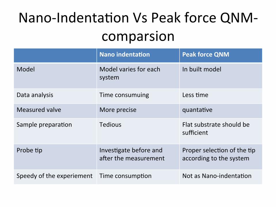
Nano-‐Indenta-on Vs Peak force QNM-‐ comparsion Nano indenta:on Peak force QNM

Model Model varies for each system

In built model

Data analysis Time consumuing Less -me

Measured valve More precise quanta-ve

Sample prepara-on Tedious Flat substrate should be sufficient

Probe -p Inves-gate before and a_er the measurement

Proper selec-on of the -p according to the system

Speedy of the experiement Time consump-on Not as Nano-‐indenta-on

Conclusions

Nanoindenta-on by AFM technique is very useful technique to precisely measure the mechanical proper-es of 2D structures compared to conven-onal test where their values are dominated by the defects, stalking faults and grain boundary in the 3D structures or nano tubes Peak Force QNM is an useful technique for samples where there are two or three mixtures of components for example a bio-‐molecule between two nanosheets, mixtures of nanosheets , mul--‐layer films or surface termina-on in pervoskites etc

Documents

Mechanical)proper-es)of) nanosheets)by)AFM)