Contents lists available at ScienceDirect

Mechanical Systems and Signal Processing

Mechanical Systems and Signal Processing 84 (2017) 241–264

http://d0888-32

n CorrE-m

journal homepage: www.elsevier.com/locate/ymssp

Parametric system identification of resonantmicro/nanosystems operating in a nonlinear response regime

A.B. Sabater, J.F. Rhoads n

School of Mechanical Engineering, Birck Nanotechnology Center, and Ray W. Herrick Laboratories, Purdue University, West Lafayette, IN47907, USA

a r t i c l e i n f o

Article history:Received 2 June 2015Received in revised form22 November 2015Accepted 6 June 2016Available online 22 July 2016

Keywords:Parametric system identificationNonlinearResonanceMicrocantileverMicro/nanosystemsAveragingPerturbation theoryHarmonic balanceMEMSNEMS

x.doi.org/10.1016/j.ymssp.2016.06.00370/& 2016 Elsevier Ltd. All rights reserved.

esponding author.ail addresses: asabater@purdue.edu (A.B. Sab

a b s t r a c t

The parametric system identification of macroscale resonators operating in a nonlinearresponse regime can be a challenging research problem, but at the micro- and nanoscales,experimental constraints add additional complexities. For example, due to the small andnoisy signals micro/nanoresonators produce, a lock-in amplifier is commonly used tocharacterize the amplitude and phase responses of the systems. While the lock-in enablesdetection, it also prohibits the use of established time-domain, multi-harmonic, and fre-quency-domain methods, which rely upon time-domain measurements. As such, the onlymethods that can be used for parametric system identification are those based on fittingexperimental data to an approximate solution, typically derived via perturbation methodsand/or Galerkin methods, of a reduced-order model. Thus, one could view the parametricsystem identification of micro/nanosystems operating in a nonlinear response regime asthe amalgamation of four coupled sub-problems: nonparametric system identification, orproper experimental design and data acquisition; the generation of physically consistentreduced-order models; the calculation of accurate approximate responses; and the ap-plication of nonlinear least-squares parameter estimation. This work is focused on thetheoretical foundations that underpin each of these sub-problems, as the methods used toaddress one sub-problem can strongly influence the results of another. To provide context,an electromagnetically transduced microresonator is used as an example. This exampleprovides a concrete reference for the presented findings and conclusions.

& 2016 Elsevier Ltd. All rights reserved.

1. Introduction

There are many established uses of resonant microelectromechanical systems (MEMS) in inertial and pressure sensingapplications [1,2], as well as emerging applications such as mass sensing [3], filtering [4] and timing [5], which are enabledby the small size and low power consumption metrics associated with these systems. As these devices continue to shrink tothe nanoscale, the aforementioned advantages are often double-edged in that system characterization becomes morechallenging. For example, the dynamic range, or the range of excitations where the response is linear, decreases with areduction in scale [6], which inhibits the use of established linear characterization techniques.

System identification in the presence of nonlinearity can be a challenging problem. Due to the relevance of this problemto systems of many different scales, it has spawned a vast amount of research literature, of which a review can be found in

ater), jfrhoads@purdue.edu (J.F. Rhoads).

A.B. Sabater, J.F. Rhoads / Mechanical Systems and Signal Processing 84 (2017) 241–264242

[7]. Unfortunately, due to experimental constraints, the majority of system identification methods that have been developedcannot be used with micro/nanosystems, as a lock-in amplifier is used to acquire the typically small and noisy response ofthese systems [8–11]. This largely inhibits the use of time-domain methods, multi-harmonic methods, or frequency-domainmethods, which rely upon a time-domain measurement, as the lock-in amplifier is only capable of measuring the amplitudeand phase of a single harmonic of the steady-state response. The methods that are amenable to use when a lock-in amplifieris employed in the measurement system are based on fitting experimental data to an approximate solution of a reduced-order model. These approximate solution-based methods have applicability beyond micro/nanosystem characterization, asthey have also been applied in the parametric identification of macroscale systems [12–16]. More recent works have adaptedapproximate solution-based methods for resonant micro/nanosystems [11,17–22], but there are significant limitations. Thiswork is focused on these limitations, and more generally the conditions under which a resonant micro/nanosystem can becharacterized by approximate solution-based methods.

In order to facilitate the parametric system identification of a resonant micro/nanosystem operating in a nonlinear re-sponse regime when a lock-in amplifier is employed, several sub-problems must be addressed: nonparametric systemidentification, or experimental design and data acquisition; the generation of physically consistent reduced-order models;the calculation of accurate approximate responses; and the application of nonlinear least-squares parameter estimationmethods. This work is focused on the theoretical foundations of these sub-problems, and how each is intrinsically coupledto the others. Accordingly, a general theoretical framework is presented that is independent of the final application of theestimated parameters. Thus, while one could potentially the relax constraints that one of the sub-problems might introducebased on the final application, a common framework allows one to communicate with a larger audience, enables technicaladvancements in one application to benefit all of them, and mitigates the need for subjective expert knowledge.

Since this work is theoretical in nature, the only nonparametric system identification issue considered herein is noise. Aswill be shown in later sections, with a sufficiently accurate model, noise only influences the variability of the parameterestimates. Accordingly, the bulk of this work is focused on the latter of the three sub-problems noted above. It is importantto point out that few prior works have, as identified by the authors, considered all four major aspects of parametricallyidentifying resonant systems operating in a nonlinear response regime. A notable exception, however, that focused onmacroscale systems was [23]. In that work, a multi-term harmonic balance solution was used to produce steady-stateresponses for a model that included often-ignored, higher-than-third-order nonlinearities. Two major challenges that werealso encountered by the authors of this work were issues related to converging to the correct solution, in particular whenmultiple stable solutions were present, and the sensitivity of the fully nonlinear estimation technique to initial parameterestimates. The authors of [23] elected to use a sub-optimal cost function as the fully nonlinear estimation technique wassensitive to initial parameter estimates. A significant limitation with using a sub-optimal estimation technique is that it doesnot necessarily satisfy the requirements needed for statistical inference, such as generating confidence intervals for theparameter estimates, performing hypothesis testing to compare the estimated model to the nominal one or a lower-orderversion, or ascertaining model adequacy.

While by no means the only way of modeling resonant micro/nanosystems, reduced-order methods are often preferableover others as they can accurately describe dynamic responses in a manner that can be used with the other sub-problems.Without considering the other sub-problems, though, this notion of accuracy can be subjective. There are many ways thatthe accuracy of a reduced-order model can be improved, such as the inclusion of multiple modes, but in this work, it will beshown that differences between third-order and fifth-order models at excitations close to the critical one, or the one atwhich bistability is present in the steady-state response, can be significant enough to prohibit accurate parametric iden-tification. A common method of calculating approximate steady-state responses of a micro/nanoresonator is to use first-order perturbation methods. These methods are very useful, particularly in regards to design, as they can distill complexphenomena to something much simpler, but they can also introduce two issues: errors between the first-order solution andhigher-order or more accurate solutions and effective parameter coupling.

There are several ways of estimating system parameters based on observed responses, such as maximum-likelihoodmethods, but the most commonly used for micro/nanosystem characterization are based on least-squares methods. In thesemethods, parameter estimation results from minimizing an error function that is equal to the squared sum of the residualsbetween the model and data. A fundamental assumption is that in the absence of noise, the nominal parameters yield anerror function equal to zero. If a first-order perturbation-based solution, or more generally a deficient model, violates thiszero error function condition, the estimated parameters may not correspond to the nominal parameters (i.e. the physicalsignificance of the estimated parameters may be dubious). It is important to note that the use of a high-fidelity modelintroduces its own problems, such as the classic bias-variance issue [24]. However, since careful experimental design inconjuction with the proper use of a lock-in amplifier can significantly reduce the variability of the measured response, it ispossible to estimate parameters that correspond to a high-fidelity model to within a reasonable tolerance. In addition, inorder for the nominal parameters to minimize the error function, the error function's Hessian, evaluated with the nominalparameters, must be positive definite. If the first-order perturbation-based solution effectively couples parameters together,this positive definite condition is violated. Note that this issue of effectively coupled parameters is not limited to pertur-bation-based solutions, and can occur with any solution when its corresponding error function's Hessian is not positivedefinite.

The starting point for this research related to the parametric system identification of resonators operating in a nonlinearresponse regime arose from characterizing microscale cantilevers. Accordingly, Section 2 presents a fifth-order model for an

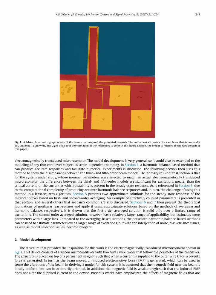
Fig. 1. A false-colored micrograph of one of the beams that inspired the presented research. The entire device consists of a cantilever that is nominally350 μm long, 75 μm wide, and 2 μm thick. (For interpretation of the references to color in this figure caption, the reader is referred to the web version ofthis paper.)

A.B. Sabater, J.F. Rhoads / Mechanical Systems and Signal Processing 84 (2017) 241–264 243

electromagnetically transduced microresonator. The model development is very general, so it could also be extended to themodeling of any thin cantilever subject to strain-dependent damping. In Section 3, a harmonic-balance-based method thatcan produce accurate responses and facilitate numerical experiments is discussed. The following section then uses thismethod to show the discrepancies between the third- and fifth-order beam models. The primary result of that section is thatfor the system under study, whose nominal parameters were selected to match an actual electromagnetically transducedmicroresonator, the differences between the third- and fifth-order models are significant for excitations greater than thecritical current, or the current at which bistability is present in the steady-state response. As is referenced in Section 3, dueto the computational complexity of producing accurate harmonic balance responses and, in turn, the challenge of using thismethod in a least-squares algorithm, Section 5 presents two approximate solutions for the steady-state response of themicrocantilever based on first- and second-order averaging. An example of effectively coupled parameters is presented inthat section, and several others that are fairly common are also discussed. Sections 6 and 7 then present the theoreticalfoundations of nonlinear least-squares and apply it using approximate solutions based on the methods of averaging andharmonic balance, respectively. It is shown that the first-order averaged solution is valid only over a limited range ofexcitations. The second-order averaged solution, however, has a relatively larger range of applicability, but estimates someparameters with a large bias. Compared to the averaging-based methods, the presented harmonic-balance-based methodscan be used to estimate parameters over a larger range of excitations, but with the interjection of noise, bias-variance issues,as well as model selection issues, become relevant.

2. Model development

The structure that provided the inspiration for this work is the electromagnetically transduced microresonator shown inFig. 1. This device consists of a silicon microcantilever with two Au/Cr wire traces that follow the perimeter of the cantilever.The structure is placed on top of a permanent magnet, such that when a current is supplied to the outer wire trace, a Lorentzforce is generated. In turn, as the beam moves, an induced electromotive force (EMF) is generated, which can be used tosense the vibrations of the beam. In deriving a model for this system, it is assumed that the magnetic field near the beam islocally uniform, but can be arbitrarily oriented. In addition, the magnetic field is weak enough such that the induced EMFdoes not alter the supplied current to the device. Previous works have emphasized the effects of magnetic fields that are

Fig. 2. Schematic diagram of the beam element and dynamic variables used for modeling [28].

A.B. Sabater, J.F. Rhoads / Mechanical Systems and Signal Processing 84 (2017) 241–264244

parallel to the beam [25], but tangential magnetic fields can be used to parametrically excite the beam [26–28] as well. Sincethis device was tested in a vacuum chamber, in an attempt to reduce viscous damping effects, the amplitude of the currentneeded to observe responses in a nonlinear response regime was relatively small. The authors of this work have consideredthe dynamic response of similar devices [11], but in the noted effort, the excitations were limited to near the onset of thenonlinear response regime. In order to observe responses in that regime, significant effort was required to mitigate noise-related issues with the excitation and measurement systems. Thus, a motivation for the study of electromagneticallytransduced microresonators, and more generally micro/nanoresonators, operating in a nonlinear response regime is that itallows one to mitigate these experimental problems [6].

The model developed here is very similar to the ones presented in previous works [28,29–31], however, it has beenmodified to include effects related to nonlinear damping. The need for the model to account for nonlinear damping is basedon experimental results, however, since nonlinear damping is not the focus of the present work, the justification for it isrelegated to Appendix A. It is assumed that all damping effects are small, viscous damping is insignificant, and that thesource of dissipation is strain-dependent viscoelastic effects. Similar work has been done on modeling thin cantileverssubject to viscoelastic damping [32], but the current work attempts to account for the total nonconservative moment andnot just the contribution that directly affects the transverse displacement.

One of the fundamental assumptions of modeling thin beams is that bending is due to moments applied to the beam. Putin a mathematical context,

ψϵ = − ′ ( )z , 1s

where ϵs is the axial strain in the beam, z is the distance from the neutral axis of the beam, ψ is defined in the schematic ofthe beam element in Fig. 2, and (•)′ denotes a derivative with respect to the arc length variable s. Assuming a Kelvin–Voigtmaterial model [33], stress and strain are related by

σ = ϵ + ϵ ( )E G , 2s s s

where ss is the axial stress in the beam, E is the modulus of elasticity, G is the loss modulus, and (•) denotes a derivative withrespect to time. In turn, the bending moment is given by

∬ σ ψ ψ= = − ( ′ + ′) ( )M z A I E Gd , 3As

where A is the particular cross section under study and I is the cross-sectional moment of inertia. Therefore, the totalmoment can be said to be due to the sum of the conservative and nonconservative moments, and it is this nonconservativemoment from which nonlinear damping arises. Further details on the selection of the Kelvin-Voigt material model can befound in Appendix A.

With Eq. (3) in hand, a reduced-order model for the dynamics of a thin cantilever beam can be derived using variationalprincipals. To do this, a specific Lagrangian L is defined as

ρ ψ¯ = + − ′ ( )⎡⎣ ⎤⎦L A u v EI

12

12

, 42 2 2

where u and v are defined in Fig. 2 as the longitudinal and transverse displacements, respectively, and ρ and A are the massdensity and cross-sectional area, respectively. It is important to note that this particular Lagrangian prohibits the in-vestigation of certain dynamic phenomena, like torsional vibrations or out-of-plane motion, but previous works haveconsidered flexural–flexural–torsional vibrations [29,30]. The assumption of ignoring torsional vibrations is experimentallygrounded, as the first bending and torsional modes of the microcantilever shown in Fig. 1 are significantly spaced. Thesemodes were recorded at 22.7 kHz and 209.3 kHz, respectively, with a Polytec MSA-400 laser Doppler vibrometer. Since themicrocantilever was designed to be weakly sensitive to out-of-plane Lorentz forces and the MSA-400 was not configured tomeasure motion parallel to the surface it was interrogating, no out-of-plane modes were measured. Effects related tobending due to shear and in-plane torsional inertia that are accounted for in Timoshenko beam models are also neglected asit is assumed that the beam is thin. In addition, the microcantilever shown in Fig. 1 is assumed to be narrow such that platedynamics can be ignored and the mechanical effects of the two wires along its perimeter are insignificant. These wire traces

A.B. Sabater, J.F. Rhoads / Mechanical Systems and Signal Processing 84 (2017) 241–264 245

are assumed to be small, but if the device was modified such that the wires were coiled or the beamwas much wider, whichmight be done to decrease the current needed to actuate the beam and increase the induced EMF due to vibrations, thespecific Lagrangian may need to be modified [35,36,19].

This specific Lagrangian can be used in conjunction with the extended Hamilton's principle to yield the variationalequation of motion for the system:

∫ ∫ ∫ ∫ { }δ δ λ δ δ δψ= = ¯ + − ( + ′) − ( ′) + + + ′( )

ψ ′⎧⎨⎩

⎡⎣ ⎤⎦⎫⎬⎭H L u v s t Q u Q v Q s t0

12

1 1 d d d d ,5t

t l

t

t l

u v0

2 2

01

2

1

2

where l is the undeformed length, λ is a Lagrange multiplier used to enforce an inextensibility constraint, Qu and Qv are thenonconservative forces in the longitudinal and transverse directions, respectively, and ψ′Q is the nonconservative momentapplied to the beam. Note that the nonconservative forces and moment are assumed to be zero at the fixed and free ends ofthe cantilever such that these effects do not need to be accounted for in the boundary conditions. These nonconservativeforces and moment, however, must be present to account for both the forces used to actuate the cantilever and effectsrelated to dissipation.

Dissipation in micro/nanosystems is a rather complex and diverse field, as it requires knowledge of many differentdisciplines [37,38], but in this effort, as previously noted, it is assumed that all damping effects are strain dependent.Specifically, all damping is assumed to be due to the viscoelastic behavior of the beam's material. The reason for thisassumption is that it can account for experimentally observed nonlinear damping, not only with the system being modeled,but with other nanoresonators operated such that viscous damping is negligible (i.e. operation in vacuum) [39,21,22].Damping due to viscoelastic behavior has been considered before [40], and it is possible that other loss mechanisms, such asthermoelastic damping or clamping loss, could also contribute to nonlinear damping mechanisms. The broader goal,however, is to show that any damping effects that are strain dependent will result in a system with nonlinear damping, andthat by using the model that will be subsequently presented, an estimate for the influence of nonlinear damping can beascertained from how strong the linear damping is. That is, in an experimental context, if the excitations are limited suchthat nonlinear effects are small, a quality factor that captures the total contributions of linear damping effects can beextracted. This quality factor can then be used to estimate the loss modulus, provided loss mechanisms are linearly de-pendent on strain as in the previously discussed model. In turn, this loss modulus can then be used to estimate the influenceof nonlinear damping.

It is possible to manipulate Eq. (5) such that the inclusion of the nonconservative moment alters the nonconservativeforces. By integrating the term with ψ′Q by parts,

∫ ∫ ∫ ∫

∫ ∫

δψ δψ ψ δ ψ δ

ψ δ ψ δ

′ = − ′ ∂∂ ′

+ ′ ∂∂ ′

+ ′ ∂∂ ′

′ + ′ ∂∂ ′

′( )

ψ ψ ψ ψ

ψ ψ

′ ′ ′ ′

′ ′

⎧⎨⎩⎡⎣⎢

⎤⎦⎥

⎡⎣⎢

⎤⎦⎥

⎫⎬⎭⎧⎨⎩

⎡⎣⎢

⎤⎦⎥

⎡⎣⎢

⎤⎦⎥

⎫⎬⎭

Q s t Q t Qu

u Qv

v t

Qu

u Qv

v s t

d d d d

d d .6

t

t l

t

t l

t

t l

t

t l

0 0 0

0

1

2

1

2

1

2

1

2

If ideal cantilever boundary conditions are assumed, the boundary terms vanish, and the end result is that the non-conservative moment effectively adds to the nonconservative forces. From this point forward, the rest of the reduced-ordermodel derivation parallels [28], but a complete derivation follows.

Integrating Eq. (5) by parts, and assuming that effects related to the nonconservative moment have been included in thenonconservative forces, the variation of the Hamiltonian can be rewritten as

∫ ∫ ∫ ∫

∫ ∫ ∫

{ } { }

{ }

δ ρ δ ρ δ

ρ δ δ δ δ ψ ψ ψ δ

= − ¨ + + ′ + − ¨ + + ′

+ [ + ] + − − + − ′∂∂ ′

′′

+ ∂∂ ′

′( )

′ ′

′ ′⎡⎣⎢

⎛⎝⎜

⎞⎠⎟

⎤⎦⎥

H Au Q G u s t Av Q G v s t

A u u v v s G u G v t EIu

dudv v

v t

d d d d

d d d ,7

t

t l

u ut

t l

v v

l

t

t

t

t

u v

l

t

tl

0 0

0 0 0

1

2

1

2

1

2

1

2

1

2

where

ψ ψ λ

ψ ψ λ

= − ″∂∂ ′

+ ( + ′)

= − ″∂∂ ′

+ ′ ( )

′

′

G EIu

u

G EIv

v

1 ,

. 8

u

v

In order for the variations of u and v to be arbitrary, the terms proportional to their respective variations yield twocoupled partial differential equations

ρ ψ ψ λ

ρ ψ ψ λ

= ¨ + ″∂∂ ′

− ( + ′)′

= ¨ + ″∂∂ ′

− ′′

( )

⎡⎣⎢

⎤⎦⎥

⎡⎣⎢

⎤⎦⎥

Q Au EIu

u

Q Av EIv

v

1 ,

.9

u

v

A.B. Sabater, J.F. Rhoads / Mechanical Systems and Signal Processing 84 (2017) 241–264246

The last three terms of Eq. (7) yield initial and boundary conditions, which will be assumed to be approximately satisfied.Using the kinematic constraint that there is no bending due to shear forces,

ψ = ′+ ′ ( )v

utan

1,

10

and the inextensibility constraint,

′ + ( + ′) = ( )v u1 1, 112 2

u and ψ can be approximated to fifth-order as

ψ

′ ≈ − ′ − ′ + ( ′ )

≈ ′ + ′ + ′ + ( ′ ) ( )

u v v O v

v v v O v

12

18

,

16

340

. 12

2 4 6

3 5 7

The results from Eq. (12) can then be used with the first equation in Eq. (9) to calculate an approximate Lagrange multiplier

∫ ∫ ∫ ∫ ∫ ∫

∫ ( )

λ ρ ρ ρ≈ − ¨′ − ¨′ − ′ ¨′

− + ′ + ′ − ′ ‴ + ′ ″ + ′ ‴( )

⎛⎝⎜

⎞⎠⎟

A v s s A v s s Av v s s

v v Q s EI v v v v v v

12

d d18

d d14

d d

112

38

d .13

l

s s

l

s s

l

s s

l

s

u

02

1 20

41 2

20

21 2

2 41

2 2 3

2 2 2

The approximate Lagrange multiplier can then be used in the second equation of Eq. (9) to yield a single partial dif-ferential equation that describes the transverse displacement of the beam

∫ ∫

∫ ∫ ∫ ∫

∫ ∫ ∫ ∫

ρ ρ

ρ ρ ρ

ρ ρ

¨ + + ″ + ′ ″ ‴ + ′ + ′ ″ + ′ ″ ‴ + ′ + ″ ′

+ ′ ′ + ″ ′ + ′ ′

+ ′ ″ ′ + ′ ′ + ″ + ′ ″ + ′ ″

+ ′ + ′ + ′ =( )

⎡⎣ ⎤⎦ ⎡⎣ ⎤⎦

⎛⎝⎜

⎞⎠⎟

⎛⎝⎜

⎞⎠⎟

Av EIv EI v v v v v v EI v v v v v v v Avddt

v s s

Avddt

v s Avddt

v s s Avddt

v s

Av vddt

v s s Avddt

v s v v v v v Q s

v v v Q Q

4 6 812

d d

12

d18

d d18

d

34

d d14

d32

158

d

12

38

.14

iv iv iv

l

s s

s

l

s s s

l

s s s

l

s

u

u v

3 2 2 3 3 42

2 02

1 2

2

2 02

1

2

2 04

1 2

2

2 04

1

22

2 02

1 23

2

2 02

12 4

1

3 5

2

2

2

Before proceeding to deriving the reduced-order model, the nonconservative forces can be introduced into the governingequation. For this particular model, the Lorentz force is assumed to only interact with the beam near its free end, but for amore general model, different force profiles can be introduced at this stage. The nonconservative forces on the beam,including viscoelastic effects, are

δ ψ

δ ψ

= ( ) ( − ) + ″ ′ ′

= − ( ) ( − ) + − ″( + ′) ′ ( )

⎡⎣ ⎤⎦⎡⎣ ⎤⎦

Q gB i t s l GI v

Q gB i t s l GI u

,

1 , 15

u y

v x

where Bx and By are the components of the magnetic field in the x and y directions, respectively, δ ( )s is the Dirac deltafunction and i(t) is the current supplied to the beam. Note that the delta functions are applied an infinitesimal distance fromthe free end of the beam such that the boundary conditions are not modified. Furthermore, in the schematic of the beamshown in Fig. 2, current is flowing into the page at the tip of the beam.

To help facilitate analysis, Eq. (14) can be nondimensionalized such that

^ = ^ = ^ =( )

vvv

ssl

ttT

, , ,160

where v0 is the thickness of the beam and

ρ=( )

TAlEI

.17

4

By assuming a single-mode expansion for the dimensionless displacement

( ) ( ) ( )Ψ^ ^ ^ = ^ ^( )v s t z t s, , 18

where ( )Ψ s solves the dimensionless boundary value problem for the first bending mode of an ideal cantilever, and re-

scaling dimensionless time again, a reduced-order model can be derived

Table 1Numerical values used in the subsequently presented numerical experiments as the nominalparameters of Eq. (19).

=k 3.271273λ = −

gB l

EIv0.375962 Ay

1

4

02

1

=k 17.32405λ = −

gB l

EIv1.16482 Ay

3

4

02

1

β = 4.59677λ = −

gB l

EIv5.82913 Ay

5

4

02

1

ν = 51.26071=Q

ETv

Gl0.284413 0

2

2

ν = 25.63042 γ = GET

17.25283

η = − −gB l

EIv0.161781 Ax

1

5

03

1 γ = GET

162.4305

A.B. Sabater, J.F. Rhoads / Mechanical Systems and Signal Processing 84 (2017) 241–264 247

( )λ τ λ τ γ β λ τ γ ν

ν η τ

″ + ϵ′ + + ϵ ( ) + ϵ + ϵ ( ) + ϵ ′ + ϵ ′ + ″ + ϵ + ϵ ( ) + ϵ ′ + ϵ ′

+ ϵ ″ = ϵ ( ) ( )

⎡⎣ ⎤⎦ ⎡⎣ ⎤⎦ ⎡⎣ ⎤⎦zQ

z i z k i z z z zz z z k i z z z z z

z z i

1

, 19

1 32

33

32 2 2 2

53

55 2

54 2

13 2

22

41

where ϵ = ( )v l/02 and the rest of the parameters are defined in Tables B1 and B2. Numerical values for the parameters in Eq.

(19) are given in Table 1. The current supplied to the microcantilever is assumed to be of the form

τ Ωτ( ) = ( ) ( )i i cos , 200

where i0 is the amplitude of the supplied current and Ω is the dimensionless ratio of the excitation frequency to themicrocantilever's first natural frequency. That is, assuming the excitation frequency is defined as fd in Hertz, then

Ωπω

=( )

Tf2.

21d

0

As will be shown in the following section, an approximate solution for Eq. (19) can be found via the method of averaging.This method, however, requires a small scaling value. The parameter ϵ, which is the square of the beam's aspect ratio, is anatural choice for this parameter, as it allows one to relate a physical quantity, the aspect ratio, to how nonlinear the beam'sresponse is to a given excitation. Assuming that the aspect ratio is small, then Eq. (19) can be said to describe a weaklynonlinear resonator [41]. Often this parameter ϵ is referred to as a “bookkeeping” parameter and is used to denote thatcertain values in the governing equation are small, but in many efforts that use perturbation-based parametric systemidentification methods, ϵ is assumed to be unity. For first-order perturbation methods, this assumption has a small influenceon the accuracy of the approximate solution, but with the second-order method that will be derived, assuming ϵ = 1 canprohibit parameter estimation. Explicitly, a selection of ϵ = 1 can yield error functions with rank-deficient approximateHessians. Beyond prohibiting parameter estimation, it is possible that the interplay between the selection of a too large ϵand the approximate form ofΩ can also introduce spurious steady-state responses to second-order solutions that have an ϵdependence [42]. The appropriate selection of ϵ also seems to be an important aspect of modeling micro/nanosystems ingeneral, as this scaling was needed with the harmonic-balance-based identification methods presented in Section 7.

At this juncture, it is important to note that it is assumed that only a single mode is excited. Since, in general, a Galerkinsolution tends to converge to the true solution as the number of modes increases to infinity, this implies that an infinitenumber of modes are excited. The relative influence of higher-order modes may be small, but as will be shown in thefollowing section, the relative discrepancies between the third- and fifth-order versions of Eq. (19) can also be small. One ofthe purposes of this work, however, is to highlight that often neglected effects can complicate or prohibit parametric systemidentification. Most of this effort focuses on approximate solution and reduced-order model selection, but future works mayassess how the inclusion or exclusion of higher-order modes influences parametric system identification of micro/nano-systems operating near their primary mode.

3. Numerical experiment design

In order to test a given parametric system identification method's capabilities, it is important to have benchmarks or stan-dards. While this assessment could be done with experimental data, this requires the control of well known issues, such as noise,and less well known issues, such as excitation frequency sweep rate and response bias due to the lock-in amplifier's low-passcharacteristics. As such, the authors have elected to use numerical experiments for validation within this work. A significantcontributing factor for this choice was also the ability to control the underlying model of the system generating the data.

A.B. Sabater, J.F. Rhoads / Mechanical Systems and Signal Processing 84 (2017) 241–264248

Generation of the data for these numerical experiments requires accurate approximate solutions to Eq. (19). To this end,the method selected was one similar to the harmonic balance method in [43], except thatΩwas the continuation parameterand a few other modifications were introduced to reduce computational complexity. That is, by rescaling time such thatsolutions are π2 periodic, which aids in simplifying the sampling requirements that are subsequently discussed, and as-suming that even harmonics do not contribute to the solution (which is not only expected, as Eq. (19) does not possess anyeven nonlinearities, but was also validated with a different set of numerical experiments), the solution to Eq. (19) wasassumed to be of the form

{ }∑τ τ τ( ) = ([ − ] ) + ([ − ] )( )=

x C n S ncos 2 1 sin 2 1 .22n

N

n n1

Provided N is large enough, the relative error of this method is small. Since the application of this model is for micro/nanosystems sensed using a lock-in detection method, only the first-harmonic of the steady-state response is of interest,thus the steady-state amplitude response is defined as

= + ( )a C S . 2312

12

A detailed explanation of how to find the values of Cn and Sn that satisfy Eq. (19) can be found in [43], but a succinctexplanation follows. Note that the foundations of the method are described in Refs. [44–46]. First, Eq. (19) is modified suchthat it is equal to zero. Then, for a given set of Cn and Sn, a sampled version of this equation is generated. Next, a discreteFourier transform is performed to estimate the Fourier coefficients of the sampled equation. A solution is found when these

N2 coefficients are all equal to zero, so the process of selecting a set of Cn and Sn is repeated until a solution converges. Anadvantage of this discrete Fourier transform based method is the ease of increasing or decreasing the number of harmonicsin a given approximate solution. A limitation of this method is that it does not allow one to analytically calculate theJacobian of the system of equations one solves to get a given solution, which is important in a parametric identificationmethod, as this Jacobian is used, in part, to calculate solution sensitivities.

One of the motivating reasons for using continuation methods is that, near turning points, the Jacobian of the system ofequations for the Cn and Sn becomes singular, thus an additional equation is introduced such that the Jacobian is no longersingular. For the harmonic balance method implemented for this work, this equation was of the form

∑Ω Ωσ

Δ = ( − ) + ( − ) + ( − )( )=

⎡⎣ ⎤⎦sN

C C S S2

,24scale n

N

n n n n2

02

21

02

02

where the subscript 0 denotes the previously found solution and the scaling factor sscale, which is needed to aid the con-vergence of the method, is defined as

∑σΩ

= +( )=

C S1

.25

scalen

N

n n1

2 2

To determine the stability of a given solution, Floquet theory was used. Classically, as was done in [43], this amounts todetermining the eigenvalues of the monodromy matrix, or characteristic multipliers. If these characteristic multipliers allhave a magnitude less then one, then the system is stable, and if this is not true, then the solution is unstable. However,calculating the monodromy matrix via numerical integration can take as long or longer than calculating its associatedharmonic balance solution. Instead, a harmonic-based method for computing stability that is founded on computing theeigenvalues of the associated Hill matrix problem is used [47].

In the numerical experiments, Δ =s 0.02, N¼10 and stable and unstable solutions are denoted by solid and dashed lines,respectively. The justification for the large N used is that accuracy is paramount. For the largest excitation considered, the C9,S9, C10 and S10 terms were on the order of 10�16 or less. The closeness of the 9th and 10th terms suggests that the Cn and Snfor N¼10 are as accurate as can possibly be obtained by the current method and are limited by numerical issues. Moregenerally, Refs. [44–46] argue that if certain conditions are met, then the harmonic balance solution uniformly converges tothe exact solution for sufficiently high N. The first condition is that the solution must be isolated, or has non-unitarycharacteristic multipliers. The second condition is that if the differential equation can be written as a series of first-orderdifferential equations of the form = ( )x X x t, , the function X must have first-order derivatives with respect to both time andthe spatial variables. The criteria of a sufficiently high N may seem nebulous, but these references also provide methods ofestimating the error of the harmonic balance solution for a finite value of N. Using Stoke's error estimate [46], the error ofthe harmonic balance solution is less than twice the product of the residual of the harmonic balance solution and a termthat is referred to asM. Definitions of the residual and thisM that are useful for calculation can be found in [45], but as notedby Stokes, for a sufficiently high number of harmonics in the harmonic balance solution, this M converges to a finite value.Thus, the term that dominates the error of the harmonic balance solution is its residual. For clarity and for the specificsystem being studied, the residual is defined as a constant that must be greater than the maximum difference between theleft- and right-hand sides of Eq. (19). The subtle point to this is that both the previously referenced terms vary with time.

Fig. 3 shows the residual of the harmonic balance solution as a function of the parameter N, as defined in this work, for

Fig. 3. A plot of the residual of the harmonic balance solution as a function of N, or the number of harmonics used in the approximate solution, for thelargest excitation case considered in this work.

A.B. Sabater, J.F. Rhoads / Mechanical Systems and Signal Processing 84 (2017) 241–264 249

the largest excitation case considered in this work, and with the nominal parameters. For N¼8 and larger, this residual tendsto reach a very small minimum value. As will be shown in a later section, in cases where the residuals between the harmonicbalance solution and ones based on averaging are much greater than the one corresponding to the N¼10 harmonic balancesolution, the authors of this work argue that these differences are due to inaccuracies of the averaged solutions. One wouldbe correct to point out that an N¼10 harmonic balance solution is not computationally efficient, and that the convergence ofthe residual to a small finite value implies that the accuracy of the harmonic balance solution is limited by its currentimplementation, but the selection of N¼10 was guided solely on the need for a benchmark solution where further increasesin N would yield no further increases in accuracy.

While the previously described method allows one to generate steady-state responses, typically in an experimentalcontext, one measures the response at discrete frequencies. In addition, these discrete frequencies are selected and changedbased on a need to reveal different hysteretic behavior. Therefore, the previously described harmonic balance method needsto be adapted such that steady-state responses at defined frequencies can be calculated, and in a fashion consistent with theprevious state of the microresonator. The first step in generating this data is reformulating the response using an amplitudeand phase representation, as was done in [43]. While the sine and cosine basis in this work mitigates the issue of multipleequivalent phases, the amplitude and phase representation allows the components of the response to be a smooth functionsofΩ. This smoothness is important, as it allows one to interpolate the response at specified frequencies. Next, the amplitudeand phase representation of the harmonic balance solution was sampled using a linear interpolation, and in a fashionconsistent with slow and discrete forward and reverse sweeps of the excitation frequency. The dimensionless frequencybandwidth considered was from Ω = 0.9995 to Ω = 1.001with a ΩΔ , or the change inΩ between discrete frequencies, set tobe × −2 10 5. For the nominal system discussed in the following sections, this corresponds to the excitation frequency beingdiscretely swept from approximately 11 Hz below the natural frequency of the microcantilever to approximately 22 Hzabove the natural frequency of the microcantilever in steps of 0.4 Hz. Thus, the selection of Δ =s 0.02 provided a minimumof four responses between frequencies at which the response was interpolated at, which enabled relatively smooth inter-polations. Finally, in order to alleviate interpolation errors, the interpolated solution was then converted back into the sineand cosine basis, and was used as a starting guess for the harmonic balance solution at the specified frequency. This lastsolution was the one used to generate data and was found to be of nontrivial importance.

4. Comparison of third-order versus fifth-order beam models

Many of the classic works on the nonlinear dynamics of cantilever beams only consider third-order nonlinearities [29–31]. Third-order models are quite useful, as with minimal adjustments to the linear theory, experimentally observedphenomena, such as the hardening or softening nature of the steady-state response or bistability, can be qualitativelypredicted. It is assumed, a priori, that third-order models are quantitatively accurate, but there are cases when higher-ordermodels are needed to even be qualitatively accurate [28]. Motivated by such findings, this section explores the differencesbetween the two models, as well as if and when these differences are significant.

Figs. 4–6 depict the steady-state amplitude response for =i 0.4, 0.70 and 1.0 mA, respectively. These three excitations willbe subsequently referred to as Cases 1, 2 and 3, respectively. The nominal parameters that are used to generate theseresponses, and the ones that are used in the following sections for system identification, are ϵ = ( )2/350 2, ϵ =Q / 6500,

Fig. 4. The steady-state responses for Case 1 where i0 is 0.4 mA. The third- and fifth-order models are shown in red and blue, respectively. (For inter-pretation of the references to color in this figure caption, the reader is referred to the web version of this paper.)

A.B. Sabater, J.F. Rhoads / Mechanical Systems and Signal Processing 84 (2017) 241–264250

ηϵ = −2 A11 and By¼0 T. Assuming that the modulus of elasticity E is 159 GPa, and the density of silicon is 2330 kg/m3, then

for the dimensions of the beam given in Fig. 1 and the value of ηϵ 1 given, the in-plane magnetic field Bx is approximately�61 mT. The third- and fifth-order models are denoted by red and blue curves, respectively. For Case 1, shown in Fig. 4 andan example of an excitation before bistability is present in the response, there are relatively insignificant differences be-tween the two models. Based on previous works [11], using first-order averaging, the presented scaling, and ignoringnonlinear damping, the critical current, or the current at which bistability is observed in the steady-state response, is

α η=

ϵ|ϵ | |ϵ |

=

( )⎛⎝⎜

⎞⎠⎟

iQ

4 2

3

0.53 mA.

26

cr

3/43/2

3 1

Thus for currents less than this value, it is expected that the two models will agree.For currents greater than the critical current, as in Case 2 shown in Fig. 5, there are some differences between the two

models. While the error may seem to be insignificant, the difference is great enough to introduce issues with the parameterestimation method presented in the following section. As one might expect, as the excitation increases, the differencesbetween the third- and fifth-order models increase. This is shown in Fig. 6, which is for Case 3.

Since there is a need for accurate models of nonlinear resonators that can be used for parametric system identification, abalance between computational complexity and implementation must be found. As Figs. 4–6 show, third-order models may

Fig. 5. The steady-state responses for Case 2 where i0 is 0.7 mA. As in the previous figure, third- and fifth-order models are shown in red and blue,respectively. In addition, stable and unstable solutions are denoted by solid and dashed lines, respectively. (For interpretation of the references to color inthis figure caption, the reader is referred to the web version of this paper.)

Fig. 6. For Case 3, an excitation of 1.0 mA was considered.

A.B. Sabater, J.F. Rhoads / Mechanical Systems and Signal Processing 84 (2017) 241–264 251

not sufficiently describe experimental results beyond the critical excitation. Ignoring terms related to parametric excitation,the third- and fifth-order models require five and nine parameters, respectively. Given that nonlinear system identificationwith five parameters can be challenging, nine parameters can be prohibitively difficult. Thus, in the following section, anapproximate solution to the third-order model is found, but it is assumed from the onset that it may fail to accurately modelresults for currents beyond the critical one. Part of Section 7, in contrast, considers a method to estimate all nine parametersof the fifth-order model.

5. Approximate solutions using the method of averaging

While several methods could be used to find an approximate solution to Eq. (19), the method of averaging was selectedbecause of the accuracy and efficiency of generating an approximate solution. In addition, since the steady-state amplitudepredicted by the method of averaging is found by solving a polynomial equation, the implicit function theorem can be usedto find solution sensitivities, which in turn can be used in parameter estimation algorithms. Moreover, compared to themethod described in Section 3, calculating stability and generating forward and reverse frequency sweep responses is muchmore straightforward. Before using this method, though, a coordinate transformation needs to be applied to Eq. (19) suchthat the transformed system can be written as a polynomial in ϵ. Specifically, the following constrained coordinate trans-formation is assumed:

τ τ Ωτ ϕ τ

τ τ Ω Ωτ ϕ τ

( ) = ( ) [ + ( )]

′( ) = − ( ) [ + ( )] ( )

z a

z a

cos ,

sin . 27

In conjunction with the transformation in Eq. (27), a constraint is needed such that one can solve for τ( )a and ϕ τ( )

Ωτ ϕ ϕ Ωτ ϕ= ′ ( + ) − ′ ( + ) ( )a a0 cos sin . 28

If Eq. (19) is written in the form of a weakly nonlinear resonator

″ + = ( ′ ϵ) ( )z z f z z t, , , , 29

where ( ′ ) =f z z t, , , 0 0, then the transformed version of Eq. (19) is

( )

( )Ω

Ω Ωτ ϕ Ωτ ϕ

ϕΩ

Ω Ωτ ϕ Ωτ ϕ

′ = − + − ( + ) ( + )

′ = − + − ( + ) ( + ) ( )

⎡⎣ ⎤⎦⎡⎣ ⎤⎦

a f a

af a

11 cos sin ,

11 cos cos . 30

2

2

At this junction, no approximations of Eq. (19) have been made. While ideally one might want to develop a systemidentification method that could uniquely and accurately determine all of the parameters in Eq. (19), the difficulty of systemidentification increases with the number of parameters. A much less computationally challenging problem, however, wouldbe the determination of all of the (ϵ)O parameters, except for λ1 which is related to parametric excitation. This is akin toignoring fifth-order nonlinearities, which as shown in the previous section, are relevant for excitations greater than thecritical excitation. Thus, provided the excitations are limited, but possibly beyond the critical current, an approximate

A.B. Sabater, J.F. Rhoads / Mechanical Systems and Signal Processing 84 (2017) 241–264252

solution to Eq. (19) that only considers third-order nonlinearities, and based on second-order averaging [48], could be usedto build qualitatively accurate models that have unique parameters. While Section 7 considers the use of a harmonic-balance-based methods, these methods are much more computationally demanding and are sensitive to initial parameterestimates.

In order to derive an approximate solution for Eq. (19), some additional assumptions are needed. Specifically, the di-mensionless excitation frequency is redefined as

Ω σ= + ϵ ( )1 , 31

and to second order the transformed variables are defined to be

ϕ ϕ ϕ ϕ

= + ϵ + ϵ

= + ϵ + ϵ ( )

a a a a ,

, 32

0 12

2

0 12

2

where a0 and ϕ0 are solutions to the averaged equations

ϕ

′ = ϵ + ϵ

′ = ϵ + ϵ ( )ϕ ϕ

a g g

g g

,

. 33

a a0 12

2

0 12

2

The solutions to the averaged equations are of primary interest, as it is assumed that provided ϵ is sufficiently small, thehigher-order contributions to the solution (i.e. a1) can be ignored. Thus, the averaged equations are

( )

γ η ϕ

β σ η ϕ

= −+ + ( )

=− − − ( )

( )ϕ

ga a Q i Q

Q

ga k a i

a

4 4 sin8

,

3 2 8 4 cos

8, 34

a1

33 0 1

1

33 0 1

and

()

( )

( )

γ βγ γ σ β η ϕ βη ϕ γ η ϕ η σ ϕ η ϕ

β β γ σ βσ γ η ϕ

βη ϕ γ η ϕ η σ ϕ η ϕ

= + − + + + − + +

= − + − + − − +

+ − − + −

ϕ

35

gQ

a k Q a Q a Q a a i k Q a i Q a i Q i Q i

gaQ

a k Q a k Q a Q a Q a k Q a Q a Q a i k Q

a i Q a i Q a i Q i Q

132

2 4 8 3 sin 6 sin cos 8 sin 4 cos ,

1256

12 51 20 11 96 64 48 72 cos

16 cos 40 sin 32 64 cos 32 sin .

a25

3 35

33

33 2

0 3 12

0 12

0 3 1 0 1 0 1

2 25

32 5

32 2 5 2 2 5 2

32 3

32 3 2 3

32

0 32

1

20

21

20

23 1 0

21 0 1

Careful analysis of Eq. (34) will show that with the first-order averaged solution, a set of k3 and β exist that produce thesame response, but this is not the case with the second-order averaged solution. Specifically, for the first-order averagedequations, a parameter

α β= − ( )k3 2 363 3

can be defined and will be subsequently referred to as the effective nonlinear coefficient.If this effective nonlinear coefficient or a similar one is not used when the first-order averaged solution is employed in a

least-squares fitting method, it can introduce significant issues. One way of decoupling the geometric and inertial effectswould be to also conduct static tests, but this method is not always feasible with micro/nanoresonators. In a more generalsense, similar effective nonlinear coefficients have been derived from the models of other micro/nanoresonators, likeelectromagnetically actuated microcantilevers with parametric excitation [28] and resonant microbeams with electrostaticexcitation [49]. Other effectively coupled parameters can result from transduction mechanisms, or the way by which inputsignals produce forces and in turn how displacements produce output signals. This was noted in a previous work by theauthors [11], but it is a common issue with micro/nanoresonators that use different phenomena for actuation and sensing.For example, previous works have shown the limitations of capacitive detection of micro/nanoresonators. To combat highfeedthrough currents and impedance mismatch, piezoresisitive detection is used [50]. The models for these devices requireknowledge about both the piezoresistive gauge factor and the modulus of elasticity. Based on the characterization methodsused, these parameters could not be independently determined. Thus, this issue of parameters being effectively coupled bysystem identification methods is by no means an isolated problem.

6. Approximate solution selection: fitting to model-generated data with averaged solutions

In order to demonstrate the advantages of the second-order averaged solution over the first-order averaged solution,both of these solutions were used to produce fits to data generated from the previously presented harmonic balance methodin a least-squares sense. Before results can be shown, however, some background information is requisite. An estimate of theparameters for a given model are defined as the parameters that minimize the error function

A.B. Sabater, J.F. Rhoads / Mechanical Systems and Signal Processing 84 (2017) 241–264 253

(^) = (^) (^) ( )S p R p R p , 37T

where p is a ×p 1 vector of the parameter estimates, p is the number of parameters for the corresponding model, R is the×R 1 residual column vector between the model and the data and R is the number of measurements. In general, an explicit

solution for the minimum of Eq. (37) cannot be found, so iterative methods are used. While many methods exist to solve thisproblem [51], the method used here exploits the implicit function theorem and an approximate Hessian. A Taylor seriesexpansion of Eq. (37) in the neighborhood of ⁎p , assuming that ⁎p is close to p such that the residual between the model andthe data is small, is

( ) ( ) ( )(^) ≈ ( ) + ( ) ( ) ^ − + ^ − ( ) ( ) ^ − ( )⁎ ⁎ ⁎ ⁎ ⁎ ⁎ ⁎ ⁎⎡⎣ ⎤⎦ ⎡⎣ ⎤⎦S Sp p J p R p p p p p J p J p p p2

12

2 , 38T T T

where J is the ×R p Jacobian of R and the terms in brackets are the Jacobian and approximate Hessian of the error function,respectively. One method for finding the minimum of a function is to search for a solution such that its gradient is zero andits Hessian is positive definite. Thus the minimization problem is converted to solving the following system of equations,

= (^) (^) ( )0 J p R p , 39T

subject to the constraint that its approximate Jacobian (^) (^)J p J pT must be positive definite. The requirement that the Jacobianmust be positive definite at a solution not only results from the need to find a minimum to the error function, but it also isrequired to find unique parameters. If the Jacobian is rank deficient, or close to singular, it is possible to define sets ofparameters that will yield nearly identical fits. To solve Eq. (39), MATLAB's fsolve algorithmwas used. A starting guess for theparameters is also needed, so except for a single numerical experiment, the nominal parameters were selected as the initialguess. The convergence capabilities of this method are not of primary interest, so the use of the nominal parameters ingeneral decreases the number of iterations needed for convergence. In the one experiment where the nominal parameterswere not used, a different set was specifically used to address convergence issues. While how robust a method is to poorinitial parameter estimates is important, the selection of the nominal parameters as the initial guess allows ones to in-directly investigate the biases of the estimated parameters.

Note that in the numerical experiments, the case that ϵ is set to 1 and the rest of the parameters were scaled appro-priately was considered. It was found, that for this case, this Jacobian is nearly singular such that standard nonlinearequation solvers could not be used. An application of Gu and Eisenstat's strong rank revealing QR algorithm [52], as im-plemented in [53], showed that the parameter mostly responsible for this singularity is Q. In the numerical experiments, Qwas selected to qualitatively match the ones found from experiments, thus it might be possible to set ϵ to 1 for systems withlower Qs, or identically, systems with stronger damping. The application of this research, however, is for modeling micro/nanosystems with small damping, thus, the appropriate selection of ϵ is important.

While the numerical experiments in this section were conducted without simulating noise being added to the data, giventhe distribution of the noise added to the data, it is possible to estimate the mean and standard deviation of the estimates.Specifically, assuming that noise is added to the data from the same distribution, and that this distribution has a zero meanand standard deviation of sm, then under a few other assumptions, the details of which can be found in [51], it can be statedthat the parameters found from the least-squares method are unbiased estimates of the actual parameters and that thecovariance of the parameter estimates is

σ(^) = (^) (^) ( )−⎡⎣ ⎤⎦p J p J pCov . 40m

T2 1

In practice, sm is not known a priori. Thus, the unbiased estimate of sm, or σm, is used, where

σ = (^)− ( )

SR p

p,

41m2

so in conjunction with the assumption that R is large, confidence intervals for p can be calculated from a t-distribution with−R p degrees of freedom. The authors of this work would like to note two issues with generating confidence intervals for

the parameter estimates. The first is that while Monto Carlo experiments with small levels of noise have been conducted tovalidate that under the given assumptions, p and σm belong to the expected distributions, there can be limitations with usingan approximate linearization method for calculating confidence intervals [54]. The second is that σm is an unbiased esti-mator assuming that the model is accurate. In the numerical experiments presented in this work, a case where σm issignificantly greater than sm can be indicative of an issue or issues with the associated sub-problems related to parametricsystem identification.

Much of the presented fitting method requires the Jacobian J. This Jacobian is often found approximately, such as withfinite difference methods, but it is possible to calculate the Jacobian directly using the implicit function theorem. While notshown in the previous section, it is possible to use the averaged equations to find a single polynomial equation for thesteady-state amplitude by using the trigonometric identity

ϕ ϕ= + ( )1 cos sin . 422 2

Fig. 7. The harmonic balance solution to Eq. (19) with the nominal parameters and accounting for fifth-order nonlinearities, the first-order averagedsolution with its fitted parameters, and the second-order averaged solution with its fitted parameters are shown in red, black and blue, respectively, forCase 1. Note that the green dots and magenta circles correspond to the discretely sampled harmonic balance solution for forward and reverse sweeps of theexcitation frequency, respectively. (For interpretation of the references to color in this figure caption, the reader is referred to the web version of this paper.)

A.B. Sabater, J.F. Rhoads / Mechanical Systems and Signal Processing 84 (2017) 241–264254

From the steady-state amplitude equation, which is of the form

= ( ^) ( )h a p0 , , 43

it is then possible to find the derivative of the steady-state amplitude with respect to a given parameter pi by

= − ∂∂

∂∂ ( )

dadp

hp

ha

.44i i

Figs. 7, 8 and 10, which correspond to Cases 1, 2, and 3, respectively, show the harmonic balance solutions to Eq. (19) withthe nominal parameters and accounting for fifth-order nonlinearities, the first-order averaged solution with its fittedparameters, and the second-order averaged solution with its fitted parameters, in red, black and blue, respectively. In orderto show how well the fits match the numerically generated data, green dots and magenta circles corresponding to thesampled harmonic balance solution for discrete forward and reverse sweeps of the excitation frequency, respectively, areincluded in the figures. The parameter estimates, and corresponding standard deviations, are given in Tables 2–4. In ad-dition, these tables give the value of the error function for the estimated parameters and an estimate of the standarddeviation of the noise. Note that no noise was added to the data in the numerical experiments in this section, thus theestimated noise is an artifact of issues associated with sub-optimal approaches to dealing with the sub-problems associatedwith parametric system identification.

For Case 1, as one might expect, the two fits based on the averaged solutions quantitatively match the data generated bythe harmonic balance method. This is validated numerically, since the values of the estimated noise, which are given inTable 2, are much smaller than all of the numerically generated data (i.e. the relative error is very small). The limitations ofthe two fits, however, are the significant biases between the estimated and nominal parameters. Thus, while the fittedparameters could be used in models that quantitatively match experimental results, these parameters lack physical sig-nificance. However, given that in experiments one might conduct trials with different excitation amplitudes, or morepractically, a model that is applicable for multiple excitation amplitudes is of greater utility, an excitation-dependent biassignificantly complicates the selection of parameters needed to even qualitatively match the experimental results. Thelargest relative difference between the estimated and nominal parameters for both fits comes from the γ3 estimate, which isrelated to nonlinear damping effects. The estimate for γ3 from the first-order averaged solution is particularly troublesome,as it is negative.1 The significance of nonlinear damping for excitations in that range, however, is small, which is oneexplanation as to why these fitting methods yield poor estimates.

Comparing the results of the two fits, the model based on the second-order averaged solution performs better. In Case 1,this solution yielded estimates with smaller biases. Using the results from Case 2, which are shown in Table 3, in conjunctionwith the results from Case 1, one might extrapolate that between trials, the biases of the second-order averaged modelparameters vary less than the biases of the first-order averaged model parameters. That is, provided the error function is

1 A negative third-order nonlinear damping coefficient corresponds to a system with self-excitation capabilities [55], or a condition where dampingmechanisms can add energy to the system. Thus, the issue of estimating a negative third-order nonlinear damping coefficient is twofold, in that besides theparameter estimate being significantly biased, the estimate incorrectly predicts a physical phenomena not found in the nominal system.

Fig. 8. A figure similar to Fig. 7, except for Case 2. Note that for Case 2, since the amplitude of the current supplied to the system is greater than the criticalcurrent, stable and unstable solutions are present in the steady-state response, and are denoted by solid and dashed lines, respectively.

Table 2A table of the nominal system parameters, parameter estimates, and error functions resulting from fitting the generated data to the first- and second-orderaveraged solutions for Case 1.

Nominal (ϵ)O Avg. (ϵ )O 2 Avg.

Q × −2.12245 10 1 × −2.11719 10 1 × −2.12522 10 1

± × −1.44262 10 4 ± × −1.09806 10 7

k3 3.27127 NA 5.22693

± × −2.54069 10 4

β 4.59677 NA 7.53027

± × −3.81350 10 4

η1 × −6.12500 10 A4 1 × −6.12476 10 A4 1 × −6.12500 10 A4 1

±9.03395 ± × − −5.97615 10 A3 1

γ3 × −7.54910 10 4 − × −1.05212 10 3 × −1.66898 10 3

± × −4.39020 10 4 ± × −3.44050 10 7

α3 × −6.20270 10 1 × −6.24179 10 1 × −6.20269 10 1

± × −1.92456 10 4 ± × −5.11481 10 7

(^)S p NA × −7.36553 10 5 × −3.19327 10 11

σm NA × −7.05458 10 4 × −4.66078 10 7

A.B. Sabater, J.F. Rhoads / Mechanical Systems and Signal Processing 84 (2017) 241–264 255

small, with the second-order averaged solution as the model, one might only need to conduct a few trials to generate aparametric model that quantitatively matches experimental results. This is important when testing with micro/nanosystemswhen a lock-in detection method is used, since it can take a significant amount of time to conduct a single trial. This mightnot be possible when the first-order averaged solution is employed as the approximate solution, since its correspondingerror function for Case 2 was large.

For the Case 2 responses, which are shown in Fig. 8, the differences between averaged solutions and the harmonicbalance solution may appear to be small, but the second-order averaged solution fits the data much more closely. To showthe differences between the various responses, the same responses shown in Fig. 8 are shown in Fig. 9, but over a smallerrange of excitation frequencies. It is important to note that for Case 2, the parameters for the first-order averaged solution donot actually minimize the error function, since the error of the approximate Hessian in this case is significant. It might bepossible for the first-order averaged solution to more closely match the harmonic balance solution if the exact Hessian wasused, but fundamentally the first-order averaged solution poorly models the numerical experiment.

As expected, the error of the second-order averaged solution increases as the excitation increases. Case 3 is an example ofthis. Unlike the two previous cases, the averaged solutions for Case 3, shown in Fig. 10, do not as closely mirror the harmonicbalance solution. This is highlighted in Fig. 11. In particular, the averaged solutions have the largest differences near theirrespective maximum amplitudes. This error can be described numerically, as the estimated noises, which are given inTable 4, are on par with the numerically generated data. The biases of the parameters in Table 4 may appear to be sur-prisingly small, but this is due to the use of the nominal parameters as the starting guesses. This particular case was alsoconducted using a finite-difference method for the Jacobian, since the previously mentioned approximate Hessian is

Table 3A table similar to Table 2, but for Case 2.

Nominal (ϵ)O Avg. (ϵ )O 2 Avg.

Q × −2.12245 10 1 × −2.22576 10 1 × −2.13102 10 1

± × −7.35502 10 2 ± × −6.89473 10 7

k3 3.27127 NA 5.22831

± × −1.73339 10 4

β 4.59677 NA 7.53234

± × −2.60450 10 4

η1 × −6.12500 10 A4 1 × −6.14063 10 A4 1 × −6.12499 10 A4 1

± × −3.66949 10 A2 3 ± × − −3.28912 10 A2 1

γ3 × −7.54910 10 4 × −1.90501 10 2 × −1.68953 10 3

± × −7.66647 10 2 ± × −6.94497 10 7

α3 × −6.20270 10 1 × −6.22351 10 1 × −6.20264 10 1

± × −4.03425 10 2 ± × −9.41794 10 7

(^)S p NA ×3.12047 101 × −2.26869 10 9

σm NA × −4.59176 10 1 × −3.92852 10 6

A.B. Sabater, J.F. Rhoads / Mechanical Systems and Signal Processing 84 (2017) 241–264256

inaccurate due to a significant residual. The finite-difference version of this experiment was conducted with an N¼5 har-monic balance solution as the benchmark, since for N¼10 it failed to converge after 105 iterations. The Jacobians corre-sponding to both the first- and second-order averaged solutions were rank-deficient, which at best suggests sets of para-meters for both models can be defined that can satisfy Eq. (39) and at worst suggests no solutions exist. One might be able toargue that the averaged solutions based on the third-order model qualitatively match the harmonic balance solution. Thedanger of such a statement is that this type of incorrect correlation between qualitative and quantitative match leads toparameter estimates that do not correspond to the system's reduced-order model, and thus lack any physical significance. Inaddition, the authors are unaware of statistical methods that can be applied in a case when the noise-free residual is large,so these parameters also lack statistical significance. Thus, besides the difficulties associated with finding parameter esti-mates, in general, a model that produces significant residuals between it and a more accurate one and/or has a corre-sponding error function with a rank-deficient Hessian will yield parameter estimates that lack uniqueness and significance,in both a physical and statistical sense.

7. Reduced-order model selection: fitting to model-generated data with harmonic balance solutions

In the previous section, two system identification methods based on averaging were presented. While these methods arequite computationally efficient, and generating steady-state responses to slow forward and reverse sweeps in excitationfrequency is simple, they can only be applied successfully for a limited range of excitations. In addition, some of theparameter estimates are strongly biased. As mentioned in the introduction and Section 5, there are many cases where the

Fig. 9. The same responses shown in Fig. 8, but over a smaller range of excitation frequencies so as to highlight the differences between the variousresponses.

Fig. 10. The Case 3 steady-state responses.

Fig. 11. The same responses shown in Fig. 10, except over a smaller range of excitation frequencies.

Table 4A table similar to Table 2, but for Case 3.

Nominal (ϵ)O Avg. (ϵ )O 2 Avg.

Q × −2.12245 10 1 × −2.16252 10 1 × −2.05738 10 1

± × −2.15475 10 1 ± × −1.34565 10 1

k3 3.27127 NA 3.27231

± ×2.08386 101

β 4.59677 NA 4.59382

± ×3.13021 101

η1 × −6.12500 10 A4 1 × −6.12528 10 A4 1 × −6.15264 10 A4 1

± ×9.90679 10 A3 3 ± × −6.09218 10 A3 1

γ3 × −7.54910 10 4 × −1.09870 10 2 − × −1.29205 10 4

± × −1.16776 10 1 ± × −7.14132 10 2

α3 × −6.20270 10 1 × −6.27085 10 1 × −6.29295 10 1

± × −7.13136 10 2 ± × −9.75496 10 2

(^)S p NA ×3.17104 102 ×1.11675 102

σm NA 1.46376 × −8.71603 10 1

A.B. Sabater, J.F. Rhoads / Mechanical Systems and Signal Processing 84 (2017) 241–264 257

A.B. Sabater, J.F. Rhoads / Mechanical Systems and Signal Processing 84 (2017) 241–264258

first-order averaged solution effectively couples parameters, which in turn complicates the design, characterization, andimplementation of such systems. Thus, there is need for characterization methods that can uniquely identify parameterswith small biases. This section explores the use of harmonic-balance-based methods that seek to accomplish both tasks.

Section 3 describes the method used to generate the data for the numerical experiments. In order to produce accurateapproximate solutions to Eq. (19), a high number of harmonics were used. Given the difficulty of explicitly generating thefunctions that must be solved in order to find the Cn and Sn, a discrete Fourier transform method was used. Based on theresults of the residual convergence test shown in Fig. 3, it is possible that a lower-order approximation could be used toproduce steady-state responses with relatively smaller residuals between the lower-order approximation and the higher-order approximation than between the averaged solutions and the higher-order approximation. Thus, in this section, twoN¼3 harmonic balance solutions, one for the third-order reduced order model and one for the fifth-order reduced ordermodel, which are based on solving a system of explicitly defined equations, are used to facilitate parametric systemidentification. An important reason that one would want to use explicitly defined equations is that it allows one to use theimplicit function theorem to calculate solution sensitivities.

In order to generate the system of equations used for the harmonic balance solution, MATHEMATICA was used to per-form the various substitutions, factorizations, and simplifications needed. As referenced in Section 6, the Jacobian of thesteady-state solution is needed, so the higher-order version of the implicit function theoremwas invoked. Given a system ofequations of the form

= ( ^ ^) ( )0 H CS p, , 45

where the components of the vector function H are the equations that need to be solved and CS denotes a vector of the Cnand Sn concatenated together, the sensitivities of the Cn and Sn to a particular component of p can be found by solving thefollowing linear system of equations:

∂

∂ ^

^= − ∂

∂ ( )

⎡⎣⎢⎢

⎤⎦⎥⎥

ddp p

H

CS

CS H.

46i i

Note that the term on the left and in brackets is simply the Jacobian of the vector function with respect to the Cn and Sn.When numerical experiments were conducted with the method that employs the fifth-order reduced-order model on

the cases presented in the previous section, this method failed due to a rank deficiency of the error function's approximateHessian. This failure was not caused by the relative error of the lower-order harmonic balance solution, but by deficiencies ofthe isolated cases’ sensitivity to the parameters. Using the same strong rank revealing algorithm as referenced earlier, therank deficiencies for the Cases 1 and 2 were caused by β, ν1, and ν2, and for Case 3 it was caused by just β and ν1. In order toproduce a full rank approximate Hessian, all three cases were considered simultaneously. The estimated parameters areshown in Table 5 and the fitted responses are shown in Fig. 12. In Fig. 12, the N¼10 responses used to generate the nu-merical experiment's data are shown in red, the fitted responses from the N¼3 harmonic balance solution corresponding tothe third-order reduced-order model are shown in black, and the fitted responses from the N¼3 harmonic balance solutioncorresponding to the fifth-order reduced-order model are shown in blue. As in the previous section, the numerical ex-periment's data corresponding to responses from forward and reverse sweeps in frequency are shown with green dots andmagenta circles, respectively. However, in order to not only demonstrate these methods in the presence of disturbances, butalso a model selection method, a small amount of noise was added to the data. That is, random values from a normaldistribution with zero mean and standard deviation of × −5 10 3 were added to the numerically generated data. The esti-mated parameters for both methods, as well as their corresponding error functions and noise estimates, are shown inTable 5. Finally, in regards to how the numerical experiments were setup, while the starting parameter estimates for theN¼3 harmonic balance solution corresponding to the fifth-order reduced order model were the nominal parameter esti-mates, some of the starting parameter estimates for the N¼3 harmonic balance solution corresponding to the third-orderreduced order model were slightly perturbed to address issues associated with bias and convergence. That is, the initialestimates for k3 and β were set as 5.22819 and 7.53215, respectively, as these methods are very sensitive to poor initialparameter estimates.

In order to put the aforementioned numerical experiments in context, a brief review of parameter estimation in theabsence of noise can be illustrative. When the N¼3 harmonic balance solution corresponding to the fifth-order reduced-order model was used, to within the precision reported in the tables in this work, the estimated parameters were equal tothe nominal parameters. This was due to the bias of this estimation method being relatively small. Furthermore, the noiseestimate, σm, was × −8.03322 10 12. For the parameters estimated with the third-order reduced-order model, the bias of theestimates was akin to those in Table 3 for the second-order averaged solution and the noise estimate was × −1.64532 10 3.Thus, when the standard deviation of the noise present in a given experiment is less than the previously given value, onewould expect that the fifth-order reduced-order model provides a better fit. Conversely, when the level of noise is muchgreater than this value, it may not be possible for one to determine which model provides a better fit.

With the interjection of noise, the estimated parameters corresponding to both models provide an exemplar case of theclassic bias-variance issue [24]. While the confidence intervals for the parameters corresponding to the fifth-order, reduced-order model encompass the nominal values, most of these intervals span several orders of magnitude. The relative

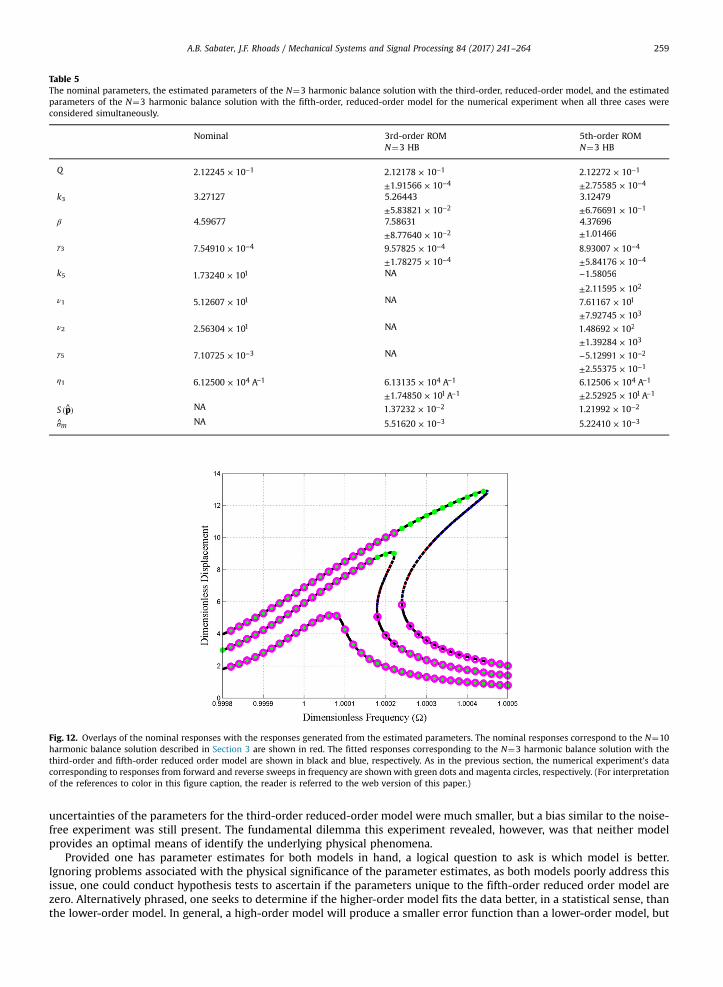
Table 5The nominal parameters, the estimated parameters of the N¼3 harmonic balance solution with the third-order, reduced-order model, and the estimatedparameters of the N¼3 harmonic balance solution with the fifth-order, reduced-order model for the numerical experiment when all three cases wereconsidered simultaneously.

Nominal 3rd-order ROM 5th-order ROMN¼3 HB N¼3 HB

Q × −2.12245 10 1 × −2.12178 10 1 × −2.12272 10 1

± × −1.91566 10 4 ± × −2.75585 10 4

k3 3.27127 5.26443 3.12479

± × −5.83821 10 2 ± × −6.76691 10 1

β 4.59677 7.58631 4.37696

± × −8.77640 10 2 ±1.01466γ3 × −7.54910 10 4 × −9.57825 10 4 × −8.93007 10 4

± × −1.78275 10 4 ± × −5.84176 10 4

k5 ×1.73240 101 NA −1.58056

± ×2.11595 102

ν1 ×5.12607 101 NA ×7.61167 101

± ×7.92745 103

ν2 ×2.56304 101 NA ×1.48692 102

± ×1.39284 103

γ5 × −7.10725 10 3 NA − × −5.12991 10 2

± × −2.55375 10 1

η1 × −6.12500 10 A4 1 × −6.13135 10 A4 1 × −6.12506 10 A4 1

± × −1.74850 10 A1 1 ± × −2.52925 10 A1 1

(^)S p NA × −1.37232 10 2 × −1.21992 10 2

σm NA × −5.51620 10 3 × −5.22410 10 3

Fig. 12. Overlays of the nominal responses with the responses generated from the estimated parameters. The nominal responses correspond to the N¼10harmonic balance solution described in Section 3 are shown in red. The fitted responses corresponding to the N¼3 harmonic balance solution with thethird-order and fifth-order reduced order model are shown in black and blue, respectively. As in the previous section, the numerical experiment's datacorresponding to responses from forward and reverse sweeps in frequency are shownwith green dots and magenta circles, respectively. (For interpretationof the references to color in this figure caption, the reader is referred to the web version of this paper.)

A.B. Sabater, J.F. Rhoads / Mechanical Systems and Signal Processing 84 (2017) 241–264 259

uncertainties of the parameters for the third-order reduced-order model were much smaller, but a bias similar to the noise-free experiment was still present. The fundamental dilemma this experiment revealed, however, was that neither modelprovides an optimal means of identify the underlying physical phenomena.

Provided one has parameter estimates for both models in hand, a logical question to ask is which model is better.Ignoring problems associated with the physical significance of the parameter estimates, as both models poorly address thisissue, one could conduct hypothesis tests to ascertain if the parameters unique to the fifth-order reduced order model arezero. Alternatively phrased, one seeks to determine if the higher-order model fits the data better, in a statistical sense, thanthe lower-order model. In general, a high-order model will produce a smaller error function than a lower-order model, but

A.B. Sabater, J.F. Rhoads / Mechanical Systems and Signal Processing 84 (2017) 241–264260

this test seeks to answer the question of if this difference is statistically significant. One test statistic one could use is thefollowing:

^ =(^ ) − (^)

(^)−− ( )

FS S

S

R pp p

p p

p,

471

1

where, as before, p is a vector of the parameter estimates corresponding to the higher-order model and p1 is a vector of theparameter estimates corresponding to the lower-order model [51]. Note that in order to calculate this test statistic, oneneeds to estimate parameters for both models. Assuming that the null hypothesis is true, or that the parameters that are

unique to the high-order model are zero, F is approximately F-distributed with −p p1 and −R p degrees of freedom, where

p1 is the length of p1. For the numerical experiments reported in Table 5, ^ =F 13.9611. The associated probability of this

occurrence (i.e. ( > ^)P F F ) is × −9.66659 10 11, which is sufficiently low that even most conservative significance levels wouldreject the null hypothesis. This might lead one to conclude that the fifth-order model is the better model. This assessment,however, is based on how the experiment was setup. With a well designed experiment, a dimensionless noise level on theorder of × −5 10 3 or smaller is obtainable. However, if experimental issues arise such that the dimensionless noise level islarger, the additional fidelity of the fifth-order reduced-order model may be unwarranted. When the level of noise was

increased to × −5 10 2, ^ = × −F 6.77104 10 1 and the associated probability of this occurrence was × −6.08117 10 1. Thus, for thecase of a poorly designed experiment, one would accept the null hypothesis.

The larger point that this section seeks to address is that the determination of the accuracy of a given parametric systemidentification is relative. The previous section sought to demonstrate that fundamentally, certain approximate solutions areflawed. However, once that issue has been addressed, the determination of the appropriate reduced-order model is con-tingent on howwell it compares to other reduced-order models. In the numerical experiments conducted in this section, theonly nonparametric system identification issue considered was noise, and it was shown that changing the level of the noisecan change which model is accepted. With poor experimental design, or in the case that the micro/nanosystem is operatingin a noisy environment, a low-fidelity model may be sufficient. Conversely, with a well designed experiment, a high-fidelitymodel is needed to mitigate issues associated with parameter estimate bias. Other challenges one might encounter in anexperimental context are issues associated with the data being biased due to how the lock-in amplifier was setup or howclose the amplitude of the microresonator is to steady-state. Comparing both lower- and higher-order models against ex-perimentally acquired results could also help one to identify these experimental issues. Thus, there is a strong utility incomparing reduced-order models, as besides providing a basis for assessment, doing so can also identify issues with theother associated sub-problems. Hopefully, this dilemma and the ones mentioned in previous sections will inspire furtherresearch on the parametric system identification of resonant micro/nanosystems that operate in a nonlinear responseregime.

8. Conclusions and future directions

Due to experimental constraints, parametric system identification of micro/nanosystems can be challenging. Specifically,since a lock-in amplifier is used, only the amplitude and phase of the measured response at a single frequency can bemeasured. Thus, many of the methods used to characterize macroscale systems are not applicable. Methods that can beused, however, are methods based on fitting the experimentally recovered response to an approximate solution. With this ismind, it is proposed that parametric system identification of resonant micro/nanosystems operating in a nonlinear regimebe decomposed into four sub-problems: nonparametric system identification, reduced-order modeling, approximate re-sponse calculation, and nonlinear least-squares parameter estimation. Due to the issues related to each of these sub-pro-blems, which were discussed in this work, this effort focused on the theoretical aspects of the last three sub-problems. Theprimary results recovered are as follows:

� At excitations close to the critical one, or at ones which hysteretic behavior can be observed in the steady-state response,discrepancies between third- and fifth-order models can prohibit accurate parameter estimation. This result is notspecifically constrained to the previously referenced model orders, and is more generally regarding model fidelity, butthird-order models are often used in attempts to explain observed responses.

� Approximate solutions that one could derive using common perturbation methods can yield significant residuals betweenthe approximate solution and a more accurate one, which again can prohibit parameter estimation. If used judiciously,however, these perturbation-based methods can be used to produce quantitatively accurate fits. The caveat with these fitsis that the parameter estimates may be significantly biased.

� Approximate solutions, or those that could be found from either perturbation methods like the method of averaging orthe harmonic balance method, can effectively couple parameters together, which besides introducing problems withstandard least-squares methods, inhibits unique parameter estimation. In this work, an example of effectively couplinggeometric and inertial nonlinearities was presented. Other notable ones can arise due to the interplay between actuationand mechanical nonlinearities or cases when different phenomena are exploited for actuation and sensing.

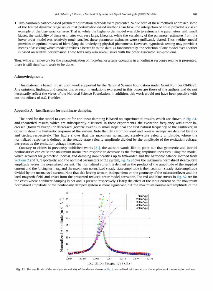
A.B. Sabater, J.F. Rhoads / Mechanical Systems and Signal Processing 84 (2017) 241–264 261

� Two harmonic-balance-based parameter estimation methods were presented. While both of these methods addressed someof the limited dynamic range issues that perturbation-based methods can have, the interjection of noise provided a classicexample of the bias-variance issue. That is, while the higher-order model was able to estimate the parameters with smallbiases, the variability of these estimates was very large. Likewise, while the variability of the parameter estimates from thelower-order model was relatively much smaller, these parameter estimates were significantly biased. Thus, neither modelprovides an optimal means of identifying the underlying physical phenomena. However, hypothesis testing may provide ameans of assessing which model provides a better fit to the data, as fundamentally, the selection of one model over anotheris based on relative performance. These tests may also reveal issues with the other associated sub-problems.

Thus, while a framework for the characterization of micro/nanosystems operating in a nonlinear response regime is presented,there is still significant work to be done.

Acknowledgments

This material is based in part upon work supported by the National Science Foundation under Grant Number 0846385.Any opinions, findings, and conclusions or recommendations expressed in this paper are those of the authors and do notnecessarily reflect the views of the National Science Foundation. In addition, this work would not have been possible without the efforts of A.G. Hunkler.

Appendix A. Justification for nonlinear damping

The need for the model to account for nonlinear damping is based on experimental results, which are shown in Fig. A1,and theoretical results, which are subsequently discussed. In these experiments, the excitation frequency was either in-creased (forward sweep) or decreased (reverse sweep) in small steps near the first natural frequency of the cantilever, inorder to show the hysteretic response of the system. Note that data from forward and reverse sweeps are denoted by dotsand circles, respectively. This figure shows that the maximum normalized steady-state velocity amplitude, where thenormalized response is defined as the steady-state velocity amplitude divided by the amplitude of the excitation voltage,decreases as the excitation voltage increases.

Contrary to claims in previously published works [21], the authors would like to point out that geometric and inertialnonlinearities can cause the maximum normalized response to decrease as the forcing amplitude increases. Using the model,which accounts for geometric, inertial, and damping nonlinearities up to fifth-order, and the harmonic balance method fromSections 2 and 3, respectively, and the nominal parameters of the system, Fig. A2 shows the maximum normalized steady-stateamplitude verses the normalized current. The normalized current is defined as the product of the amplitude of the suppliedcurrent and the forcing term ηϵ 1, and the maximum normalized steady-state amplitude is the maximum steady-state amplitudedivided by the normalized current. Note that this forcing term ηϵ 1 is dependent on the geometry of the microcantilever and thelocal magnetic field, and arises from the presented reduced-order model derivation. The red and blue curves in Fig. A2 are forthe cases where nonlinear damping is not and is present, respectively. Clearly the effect of the input current on the maximumnormalized amplitude of the nonlinearly damped system is more significant, but the maximum normalized amplitude of the

Fig. A1. The amplitude of the steady-state velocity of the device shown in Fig. 1, normalized with respect to the amplitude of the excitation voltage.

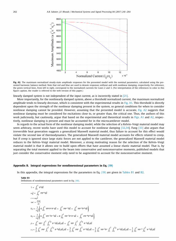
Fig. A2. The maximum normalized steady-state amplitude responses for the presented model with the nominal parameters, calculated using the pre-sented harmonic balance method. Note that red and blue are used to denote responses without and with nonlinear damping, respectively. For reference,the green vertical lines, from left to right, correspond to the normalized currents for Cases 2 and 3. (For interpretation of the references to color in thisfigure caption, the reader is referred to the web version of this paper.)

A.B. Sabater, J.F. Rhoads / Mechanical Systems and Signal Processing 84 (2017) 241–264262

linearly damped system is not independent of the input current, as is incorrectly stated in [21].More importantly, for the nonlinearly damped system, above a threshold normalized current, the maximum normalized

amplitude tends to linearly decrease, which is consistent with the experimental results in Fig. A1. This threshold is directlydependent upon the strength of the nonlinear damping present in the system, so general conditions for when to considernonlinear damping cannot be provided. However, assuming that the presented model is accurate, Fig. A2 suggests thatnonlinear damping must be considered for excitations close to, or greater than, the critical one. Thus, the authors of thiswork judiciously, but cautiously, argue that based on the experimental and theoretical results in Figs. A1 and A2, respec-tively, nonlinear damping is present and must be accounted for in the microcantilever model.

In regards to the actual form of the nonlinear damping model, while the selection of a Kelvin–Voigt material model mayseem arbitrary, recent works have used this model to account for nonlinear damping [32,34]. Fung [33] also argues thatirreversible heat generation suggests a generalized Maxwell material model, thus failure to account for this effect wouldviolate the second law of thermodynamics. The generalized Maxwell material model accounts for effects related to creep,but if creep is ignored since large static forces are not applied to the cantilever, the generalized Maxwell material modelreduces to the Kelvin–Voigt material model. Moreover, a strong motivating reason for the selection of the Kelvin–Voigtmaterial model is that it allows one to build upon efforts that have assumed a linear elastic material model. That is, byseparating the total moment applied to the beam into conservative and nonconservative moments, published models thatjust consider the conservative moment only need to be augmented to account for the nonconservative moment.

Appendix B. Integral expressions for nondimensional parameters in Eq. (19)

In this appendix, the integral expressions for the parameters in Eq. (19) are given in Tables B1 and B2.

Table B1Definitions of nondimensional parameters used in Eq. (19).

∫

∫

∫ ∫ ∫

∫ ∫ ∫

∫ ∫ ∫ ∫ ∫ ∫

∫ ∫ ∫ ∫ ∫ ∫ ∫ ∫ ∫ ∫

″ ′

′ ″ ′ ′

′ ′

′ ′ ′ ′ ′ ′

Ψ

ω ΨΨ

τ ω

τ

ωΨΨ Ψ Ψ ΨΨ ΨΨ Ψ

ωΨΨ Ψ ΨΨ Ψ Ψ ΨΨ Ψ

β ΨΨ Ψ ΨΨ Ψ

ν ΨΨ Ψ ΨΨ Ψ ΨΨ Ψ Ψ ΨΨ Ψ

= ^

= ^

= ^

(•)′ = ∂(•)∂

= ′ ″ ‴ ^ + ^ + ^

= ^ + ″ ‴ ^ + ^

= ″ ^ ^ ^ + ′ ^ ^

= ″ ^ ^ ^ + ′ ^ ^ + ″ ^ ^ ^ + ^ ^

^ ^ ^ ^

^ ^ ^ ^ ^ ^

⎛⎝⎜⎜

⎞⎠⎟⎟

⎛⎝⎜⎜

⎞⎠⎟⎟

s

s

t

k s s s

k s s s

s s s s s

s s s s s s s s s s

1 d

d

1 4 d d d

1 6 d 8 d d

d d d d d

32

d d d 32

d d 32

d d d 12

d d

iv

iv

iv

s s s s

s s s s s s

0

12

02

0

1

0

302 0

1

0

13

0

12

502 0

12 3

0

13

0

14

0

1

1 0

2 21 2

0

1

1 0

2 21

10

1

1 0

2 41 2

0

1

04

10

12

1 0

2 21 2

0

13

02

1

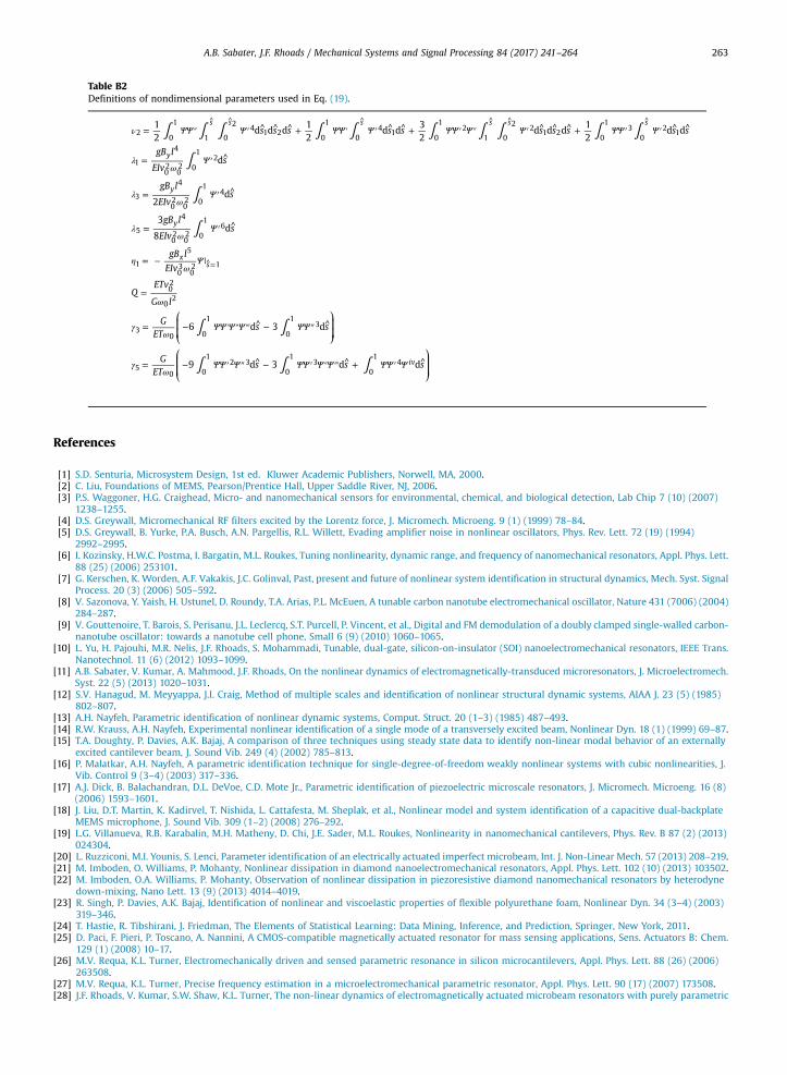
Table B2Definitions of nondimensional parameters used in Eq. (19).

∫ ∫ ∫ ∫ ∫ ∫ ∫ ∫ ∫ ∫

∫

∫

∫

∫ ∫

∫ ∫ ∫

′ ′ ′ ′ ′ ′

′

′

′

″

′ ″ ′ ′

ν ΨΨ Ψ ΨΨ Ψ ΨΨ Ψ Ψ ΨΨ Ψ

λω

Ψ

λω

Ψ

λω

Ψ

ηω

Ψ

ω

γω

ΨΨ Ψ Ψ ΨΨ

γω

ΨΨ Ψ ΨΨ Ψ Ψ ΨΨ Ψ

= ″ ^ ^ ^ + ′ ^ ^ + ″ ^ ^ ^ + ^ ^

= ^

= ^

= ^

= − |

=

= − ′ ″ ‴ ^ − ^

= − ^ − ″ ‴ ^ + ^

^ ^ ^ ^ ^ ^

^=

⎛

⎝⎜⎜

⎞

⎠⎟⎟

⎛

⎝⎜⎜

⎞

⎠⎟⎟

s s s s s s s s s s

gB l

EIvs

gB l

EIvs

gB l

EIvs

gB l

EIv

QETv

G l

GET

s s

GET

s s s

12

d d d 12

d d 32

d d d 12

d d

d

2d

3

8d

6 d 3 d

9 d 3 d d

s s s s s s

y

y

y

xs

iv

20

1

1 0

2 41 2

0

1

04

10

12

1 0

2 21 2

0

13

02

1

1

4

02

02 0

12

3

4

02

02 0

14

5

4

02

02 0

16

1

5

03

02 1

02

02

30 0

1

0

13

50 0

12 3

0

13

0

14

A.B. Sabater, J.F. Rhoads / Mechanical Systems and Signal Processing 84 (2017) 241–264 263

References

[1] S.D. Senturia, Microsystem Design, 1st ed. Kluwer Academic Publishers, Norwell, MA, 2000.[2] C. Liu, Foundations of MEMS, Pearson/Prentice Hall, Upper Saddle River, NJ, 2006.[3] P.S. Waggoner, H.G. Craighead, Micro- and nanomechanical sensors for environmental, chemical, and biological detection, Lab Chip 7 (10) (2007)

1238–1255.[4] D.S. Greywall, Micromechanical RF filters excited by the Lorentz force, J. Micromech. Microeng. 9 (1) (1999) 78–84.[5] D.S. Greywall, B. Yurke, P.A. Busch, A.N. Pargellis, R.L. Willett, Evading amplifier noise in nonlinear oscillators, Phys. Rev. Lett. 72 (19) (1994)

2992–2995.[6] I. Kozinsky, H.W.C. Postma, I. Bargatin, M.L. Roukes, Tuning nonlinearity, dynamic range, and frequency of nanomechanical resonators, Appl. Phys. Lett.

88 (25) (2006) 253101.[7] G. Kerschen, K. Worden, A.F. Vakakis, J.C. Golinval, Past, present and future of nonlinear system identification in structural dynamics, Mech. Syst. Signal

Process. 20 (3) (2006) 505–592.[8] V. Sazonova, Y. Yaish, H. Ustunel, D. Roundy, T.A. Arias, P.L. McEuen, A tunable carbon nanotube electromechanical oscillator, Nature 431 (7006) (2004)

284–287.[9] V. Gouttenoire, T. Barois, S. Perisanu, J.L. Leclercq, S.T. Purcell, P. Vincent, et al., Digital and FM demodulation of a doubly clamped single-walled carbon-

nanotube oscillator: towards a nanotube cell phone, Small 6 (9) (2010) 1060–1065.[10] L. Yu, H. Pajouhi, M.R. Nelis, J.F. Rhoads, S. Mohammadi, Tunable, dual-gate, silicon-on-insulator (SOI) nanoelectromechanical resonators, IEEE Trans.

Nanotechnol. 11 (6) (2012) 1093–1099.[11] A.B. Sabater, V. Kumar, A. Mahmood, J.F. Rhoads, On the nonlinear dynamics of electromagnetically-transduced microresonators, J. Microelectromech.

Syst. 22 (5) (2013) 1020–1031.[12] S.V. Hanagud, M. Meyyappa, J.I. Craig, Method of multiple scales and identification of nonlinear structural dynamic systems, AIAA J. 23 (5) (1985)

802–807.[13] A.H. Nayfeh, Parametric identification of nonlinear dynamic systems, Comput. Struct. 20 (1–3) (1985) 487–493.[14] R.W. Krauss, A.H. Nayfeh, Experimental nonlinear identification of a single mode of a transversely excited beam, Nonlinear Dyn. 18 (1) (1999) 69–87.[15] T.A. Doughty, P. Davies, A.K. Bajaj, A comparison of three techniques using steady state data to identify non-linear modal behavior of an externally

excited cantilever beam, J. Sound Vib. 249 (4) (2002) 785–813.[16] P. Malatkar, A.H. Nayfeh, A parametric identification technique for single-degree-of-freedom weakly nonlinear systems with cubic nonlinearities, J.

Vib. Control 9 (3–4) (2003) 317–336.[17] A.J. Dick, B. Balachandran, D.L. DeVoe, C.D. Mote Jr., Parametric identification of piezoelectric microscale resonators, J. Micromech. Microeng. 16 (8)

(2006) 1593–1601.[18] J. Liu, D.T. Martin, K. Kadirvel, T. Nishida, L. Cattafesta, M. Sheplak, et al., Nonlinear model and system identification of a capacitive dual-backplate

MEMS microphone, J. Sound Vib. 309 (1–2) (2008) 276–292.[19] L.G. Villanueva, R.B. Karabalin, M.H. Matheny, D. Chi, J.E. Sader, M.L. Roukes, Nonlinearity in nanomechanical cantilevers, Phys. Rev. B 87 (2) (2013)

024304.[20] L. Ruzziconi, M.I. Younis, S. Lenci, Parameter identification of an electrically actuated imperfect microbeam, Int. J. Non-Linear Mech. 57 (2013) 208–219.[21] M. Imboden, O. Williams, P. Mohanty, Nonlinear dissipation in diamond nanoelectromechanical resonators, Appl. Phys. Lett. 102 (10) (2013) 103502.[22] M. Imboden, O.A. Williams, P. Mohanty, Observation of nonlinear dissipation in piezoresistive diamond nanomechanical resonators by heterodyne

down-mixing, Nano Lett. 13 (9) (2013) 4014–4019.[23] R. Singh, P. Davies, A.K. Bajaj, Identification of nonlinear and viscoelastic properties of flexible polyurethane foam, Nonlinear Dyn. 34 (3–4) (2003)

319–346.[24] T. Hastie, R. Tibshirani, J. Friedman, The Elements of Statistical Learning: Data Mining, Inference, and Prediction, Springer, New York, 2011.[25] D. Paci, F. Pieri, P. Toscano, A. Nannini, A CMOS-compatible magnetically actuated resonator for mass sensing applications, Sens. Actuators B: Chem.

129 (1) (2008) 10–17.[26] M.V. Requa, K.L. Turner, Electromechanically driven and sensed parametric resonance in silicon microcantilevers, Appl. Phys. Lett. 88 (26) (2006)

263508.[27] M.V. Requa, K.L. Turner, Precise frequency estimation in a microelectromechanical parametric resonator, Appl. Phys. Lett. 90 (17) (2007) 173508.[28] J.F. Rhoads, V. Kumar, S.W. Shaw, K.L. Turner, The non-linear dynamics of electromagnetically actuated microbeam resonators with purely parametric

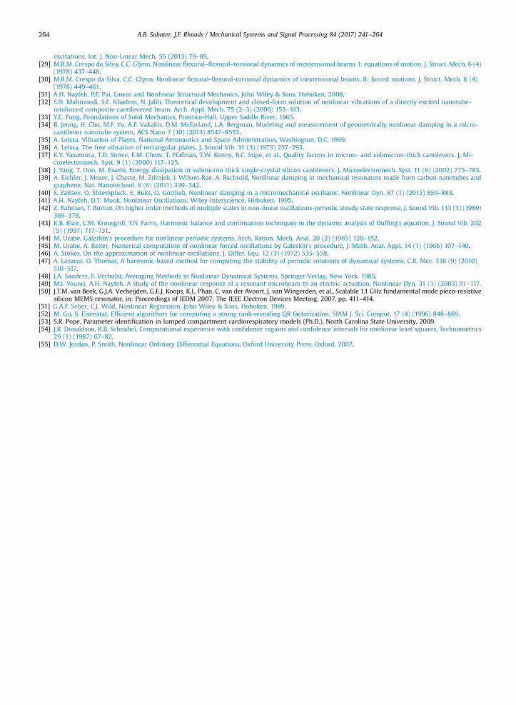
A.B. Sabater, J.F. Rhoads / Mechanical Systems and Signal Processing 84 (2017) 241–264264

excitations, Int. J. Non-Linear Mech. 55 (2013) 79–89.[29] M.R.M. Crespo da Silva, C.C. Glynn, Nonlinear flexural–flexural–torsional dynamics of inextensional beams. I: equations of motion, J. Struct. Mech. 6 (4)

(1978) 437–448.[30] M.R.M. Crespo da Silva, C.C. Glynn, Nonlinear flexural-flexural-torsional dynamics of inextensional beams. II: forced motions, J. Struct. Mech. 6 (4)

(1978) 449–461.[31] A.H. Nayfeh, P.F. Pai, Linear and Nonlinear Structural Mechanics, John Wiley & Sons, Hoboken, 2008.[32] S.N. Mahmoodi, S.E. Khadem, N. Jalili, Theoretical development and closed-form solution of nonlinear vibrations of a directly excited nanotube-

reinforced composite cantilevered beam, Arch. Appl. Mech. 75 (2–3) (2006) 153–163.[33] Y.C. Fung, Foundations of Solid Mechanics, Prentice-Hall, Upper Saddle River, 1965.[34] B. Jeong, H. Cho, M.F. Yu, A.F. Vakakis, D.M. McFarland, L.A. Bergman, Modeling and measurement of geometrically nonlinear damping in a micro-

cantilever nanotube system, ACS Nano 7 (10) (2013) 8547–8553.[35] A. Leissa, Vibration of Plates, National Aeronautics and Space Administration, Washington, D.C, 1969.[36] A. Leissa, The free vibration of rectangular plates, J. Sound Vib. 31 (3) (1973) 257–293.[37] K.Y. Yasumura, T.D. Stowe, E.M. Chow, T. Pfafman, T.W. Kenny, B.C. Stipe, et al., Quality factors in micron- and submicron-thick cantilevers, J. Mi-

croelectromech. Syst. 9 (1) (2000) 117–125.[38] J. Yang, T. Ono, M. Esashi, Energy dissipation in submicron thick single-crystal silicon cantilevers, J. Microelectromech. Syst. 11 (6) (2002) 775–783.[39] A. Eichler, J. Moser, J. Chaste, M. Zdrojek, I. Wilson-Rae, A. Bachtold, Nonlinear damping in mechanical resonators made from carbon nanotubes and

graphene, Nat. Nanotechnol. 6 (6) (2011) 339–342.[40] S. Zaitsev, O. Shtempluck, E. Buks, O. Gottlieb, Nonlinear damping in a micromechanical oscillator, Nonlinear Dyn. 67 (1) (2012) 859–883.[41] A.H. Nayfeh, D.T. Mook, Nonlinear Oscillations, Wiley-Interscience, Hoboken, 1995.[42] Z. Rahman, T. Burton, On higher order methods of multiple scales in non-linear oscillations-periodic steady state response, J. Sound Vib. 133 (3) (1989)

369–379.[43] K.B. Blair, C.M. Krousgrill, T.N. Farris, Harmonic balance and continuation techniques in the dynamic analysis of Duffing's equation, J. Sound Vib. 202

(5) (1997) 717–731.[44] M. Urabe, Galerkin's procedure for nonlinear periodic systems, Arch. Ration. Mech. Anal. 20 (2) (1965) 120–152.[45] M. Urabe, A. Reiter, Numerical computation of nonlinear forced oscillations by Galerkin's procedure, J. Math. Anal. Appl. 14 (1) (1966) 107–140.[46] A. Stokes, On the approximation of nonlinear oscillations, J. Differ. Equ. 12 (3) (1972) 535–558.[47] A. Lazarus, O. Thomas, A harmonic-based method for computing the stability of periodic solutions of dynamical systems, C.R. Mec. 338 (9) (2010)

510–517.[48] J.A. Sanders, F. Verhulst, Averaging Methods in Nonlinear Dynamical Systems, Springer-Verlag, New York, 1985.[49] M.I. Younis, A.H. Nayfeh, A study of the nonlinear response of a resonant microbeam to an electric actuation, Nonlinear Dyn. 31 (1) (2003) 91–117.[50] J.T.M. van Beek, G.J.A. Verheijden, G.E.J. Koops, K.L. Phan, C. van der Avoort, J. van Wingerden, et al., Scalable 1.1 GHz fundamental mode piezo-resistive

silicon MEMS resonator, in: Proceedings of IEDM 2007: The IEEE Electron Devices Meeting, 2007, pp. 411–414.[51] G.A.F. Seber, C.J. Wild, Nonlinear Regression, John Wiley & Sons, Hoboken, 1989.[52] M. Gu, S. Eisenstat, Efficient algorithms for computing a strong rank-revealing QR factorization, SIAM J. Sci. Comput. 17 (4) (1996) 848–869.[53] S.R. Pope, Parameter identification in lumped compartment cardiorespiratory models (Ph.D.), North Carolina State University, 2009.[54] J.R. Donaldson, R.B. Schnabel, Computational experience with confidence regions and confidence intervals for nonlinear least squares, Technometrics

29 (1) (1987) 67–82.[55] D.W. Jordan, P. Smith, Nonlinear Ordinary Differential Equations, Oxford University Press, Oxford, 2007.