Mechanical Systems and Signal Processing - · PDF fileThe complex phenomenon of hysteresis in mechanical systems motivates some researchers to explore the dynamic behavior of the systems

Contents lists available at ScienceDirect

Mechanical Systems and Signal Processing

Mechanical Systems and Signal Processing 49 (2014) 209–233

http://d0888-32

n CorrE-m

journal homepage: www.elsevier.com/locate/ymssp

Review

A survey on hysteresis modeling, identification and control

Vahid Hassani n, Tegoeh Tjahjowidodo, Thanh Nho DoNanyang Technological University, School of Mechanical and Aerospace Engineering, Division of Mechatronics & Design, 50 NanyangAvenue, Singapore 639798, Singapore

a r t i c l e i n f o

Article history:Received 22 June 2013Received in revised form27 January 2014Accepted 18 April 2014Available online 13 May 2014

Keywords:Hysteresis characterizationSmart materialsHysteresis nonlinearityParameter estimationSystem identificationHysteresis control

x.doi.org/10.1016/j.ymssp.2014.04.01270/& 2014 Elsevier Ltd. All rights reserved.

esponding author. Tel.: þ65 84317280.ail addresses: [email protected] (V. Has

a b s t r a c t

The various mathematical models for hysteresis such as Preisach, Krasnosel’skii–Pokrovs-kii (KP), Prandtl–Ishlinskii (PI), Maxwell-Slip, Bouc–Wen and Duhem are surveyed interms of their applications in modeling, control and identification of dynamical systems.In the first step, the classical formalisms of the models are presented to the reader, andmore broadly, the utilization of the classical models is considered for development ofmore comprehensive models and appropriate controllers for corresponding systems. Inaddition, the authors attempt to encourage the reader to follow the existing mathematicalmodels of hysteresis to resolve the open problems.

& 2014 Elsevier Ltd. All rights reserved.

Contents

1. Introduction . . . . . . . . . . . . . . . . . . . . . . . . . . . . . . . . . . . . . . . . . . . . . . . . . . . . . . . . . . . . . . . . . . . . . . . . . . . . . . . . . . . . . . . . . . . 2102. Hysteresis in a nutshell . . . . . . . . . . . . . . . . . . . . . . . . . . . . . . . . . . . . . . . . . . . . . . . . . . . . . . . . . . . . . . . . . . . . . . . . . . . . . . . . . . 2103. Mathematical models for hysteresis . . . . . . . . . . . . . . . . . . . . . . . . . . . . . . . . . . . . . . . . . . . . . . . . . . . . . . . . . . . . . . . . . . . . . . . . 211

3.1. Preisach model . . . . . . . . . . . . . . . . . . . . . . . . . . . . . . . . . . . . . . . . . . . . . . . . . . . . . . . . . . . . . . . . . . . . . . . . . . . . . . . . . . . 2113.2. Krasnosel’skii–Pokrovskii (KP) model . . . . . . . . . . . . . . . . . . . . . . . . . . . . . . . . . . . . . . . . . . . . . . . . . . . . . . . . . . . . . . . . . 2143.3. Prandtl–Ishlinskii (PI) model. . . . . . . . . . . . . . . . . . . . . . . . . . . . . . . . . . . . . . . . . . . . . . . . . . . . . . . . . . . . . . . . . . . . . . . . 215

3.3.1. Stop operator . . . . . . . . . . . . . . . . . . . . . . . . . . . . . . . . . . . . . . . . . . . . . . . . . . . . . . . . . . . . . . . . . . . . . . . . . . . . . 2153.3.2. Play operator . . . . . . . . . . . . . . . . . . . . . . . . . . . . . . . . . . . . . . . . . . . . . . . . . . . . . . . . . . . . . . . . . . . . . . . . . . . . . 216

3.4. Maxwell-Slip model. . . . . . . . . . . . . . . . . . . . . . . . . . . . . . . . . . . . . . . . . . . . . . . . . . . . . . . . . . . . . . . . . . . . . . . . . . . . . . . 2193.5. Bouc–Wen model. . . . . . . . . . . . . . . . . . . . . . . . . . . . . . . . . . . . . . . . . . . . . . . . . . . . . . . . . . . . . . . . . . . . . . . . . . . . . . . . . 2203.6. Duhem model . . . . . . . . . . . . . . . . . . . . . . . . . . . . . . . . . . . . . . . . . . . . . . . . . . . . . . . . . . . . . . . . . . . . . . . . . . . . . . . . . . . 220

4. System identification strategies in hysteresis characterization . . . . . . . . . . . . . . . . . . . . . . . . . . . . . . . . . . . . . . . . . . . . . . . . . . . 2214.1. Least mean square-based system identification . . . . . . . . . . . . . . . . . . . . . . . . . . . . . . . . . . . . . . . . . . . . . . . . . . . . . . . . . 2214.2. Recursive least square-based system identification . . . . . . . . . . . . . . . . . . . . . . . . . . . . . . . . . . . . . . . . . . . . . . . . . . . . . . 2234.3. Genetic algorithm-based system identification . . . . . . . . . . . . . . . . . . . . . . . . . . . . . . . . . . . . . . . . . . . . . . . . . . . . . . . . . 2234.4. System identification by particle swarm optimization (PSO) . . . . . . . . . . . . . . . . . . . . . . . . . . . . . . . . . . . . . . . . . . . . . . 2244.5. System identification by neural network . . . . . . . . . . . . . . . . . . . . . . . . . . . . . . . . . . . . . . . . . . . . . . . . . . . . . . . . . . . . . . 225

5. Control strategies in hysteretic systems . . . . . . . . . . . . . . . . . . . . . . . . . . . . . . . . . . . . . . . . . . . . . . . . . . . . . . . . . . . . . . . . . . . . . 227

sani), [email protected] (T. Tjahjowidodo), [email protected] (T.N. Do).

www.sciencedirect.com/science/journal/08883270

www.elsevier.com/locate/ymssp

http://dx.doi.org/10.1016/j.ymssp.2014.04.012



http://crossmark.crossref.org/dialog/?doi=10.1016/j.ymssp.2014.04.012&domain=pdf



mailto:[email protected]




V. Hassani et al. / Mechanical Systems and Signal Processing 49 (2014) 209–233210

5.1. Feedforward control with open-loop schemes. . . . . . . . . . . . . . . . . . . . . . . . . . . . . . . . . . . . . . . . . . . . . . . . . . . . . . . . . . 2275.2. Close-loop control with feedback information . . . . . . . . . . . . . . . . . . . . . . . . . . . . . . . . . . . . . . . . . . . . . . . . . . . . . . . . . . 2285.3. Close-loop control with a combination of feedback and feedforward . . . . . . . . . . . . . . . . . . . . . . . . . . . . . . . . . . . . . . . 229

6. Conclusion . . . . . . . . . . . . . . . . . . . . . . . . . . . . . . . . . . . . . . . . . . . . . . . . . . . . . . . . . . . . . . . . . . . . . . . . . . . . . . . . . . . . . . . . . . . . 229

1. Introduction

When speaking of hysteresis, one refers to the systems that have memory, where the effects of input to the system areexperienced with a certain delay in time. This phenomenon is originated from magnetic, ferromagnetic and ferroelectricmaterials. It is like the elastic property of materials in which a lag occurs between the application and the removal of a forceor field and its subsequent effect. The output of the system cannot be predicted without knowledge about the current stateof the hysteretic system.

The importance of this study manifests itself in a mathematical modeling of some systems that involve hysteresis such asin smart materials, magnetic fields or micro-sliding friction where hysteresis is dramatically appeared as compared to other(geometric nonlinear) systems.

Amid the smart materials, piezoceramics, one of the most researched materials, are extensively used in widespreadapplications involving vibration control [1], adaptive structural shape control [2–4], structural health monitoring [5,6],structural acoustic systems [7–9], hybrid transducers and ultrasonic motors [10,11], nanopositioning stages [12,13], andmore applications for the reason of high precision, high speed position control, high stiffness and fast response. They alsoare able to endure compressive forces up to several tons, while providing high resolutions and high bandwidth strainssimultaneously.

In addition to piezoceramics, shape memory alloys and magnetostrictive actuators are also classified in the category ofsmart materials. The application of magnetostrictive materials is reported in transducer design [14], acoustic and industrialapplications [10,15,16], and hybrid transducers [17–19].

In comparison with piezoceramics and magnetostrictive materials, shape memory alloys (SMA) are relatively newinvention of large field of smart materials [20]. SMA is widely used in industrial applications such as vibration attenuation incivil structures [21] and SMA-based microactuator [22–24], etc.

In spite of large variety of applications assigned for smart materials, they are all subjected to the main source ofnonlinearity, namely the hysteresis. This type of nonlinearity might lead to performance degradation specifically inpositioning applications. If this phenomenon is neglected, it will give rise to inaccuracy in open loop control and degradesthe tracking performance of the actuator. Also, it could cause undesirable oscillations in the systemwhich could even lead toinstability in the closed loop.

In contrast to a simple (but incomplete) representation of friction, i.e., the classical Coulomb friction modelapproximation that defines the friction force only at non-zero relative velocity (va0), in fact, micro-sliding displacementsare actually observed [25]. When a contacting body is sliding and moving away from a reversal point, the friction forcepredominantly appears as a function of velocity, similar as presented by the Coulomb model. However, when the motion isreversed, the frictional effects of the mechanism are also determined by displacement function. Therefore, at a certaininstance after the motion reversal, the friction behavior depends not only on the velocity, but also on the displacement,where the particular relation between friction and displacement involves a so-called non-local memory hysteresis [25–30].This unique behavior attracts many researchers to thoroughly model the behavior of the contact between the two surfaces,which is realized using asperity junctions that can deform elastically or plastically depending on the load and on thedisplacement and/or the relative velocity of the surfaces [31].

In high precision positioning applications, the effects of friction present in a mechanical system can lead to significantpositioning error. In order to compensate the error due to frictional forces, an effective control strategy is a prerequisite.As a consequence of the complex behavior of friction, linear control strategies are generally unsuitable for providing anoptimal performance for controlling a motion of systems with friction. If an accurate model of the system is available,a compensation of the error in the system can be made by applying a feedforward command that is equal to and opposite tothe instantaneous force.

In this paper, the various types of hysteresis models are investigated as well as their applications in modeling andcontrol. In the remaining part of this study, different types of methods which are utilized for parameter estimation, systemidentification and system control will be briefly discussed. This paper will be wrapped up by conclusion.

2. Hysteresis in a nutshell

The presence of hysteresis in ferroelectric-based materials (such as piezoelectric materials) is an important propertywhich creates constitutive nonlinearities in the relation between input fields E (V/m) and stresses s (N/m2) and outputpolarization P (C/m2) and strains ε (m/m) as illustrated in Fig. 1. As detailed in [20], hysteresis is directly associated with thenon-centro-symmetric structure of ferroelectric compounds and is observed to some degree at essentially all drive levels.

One of the main characteristics of ferroelectric materials is polarization reversal or switching by an electric field.Application of an electric field in ferroelectric materials will reduce domain walls in ceramics [20]. This phenomenon

Fig. 1. Hysteresis and switching logic in ferroelectric materials [20].

V. Hassani et al. / Mechanical Systems and Signal Processing 49 (2014) 209–233 211

(reducing and increasing in domain walls) is observed in terms of the hysteresis loop in ferroelectric materials. For furtherunderstanding, the switching phenomenon is discussed based on Fig. 1 as follows [20]:

Point A: In maximum amount of positive field, all dipoles are aligned with the field and material acts as a single domain.Increasing the field beyond this point results in the linear constitutive relations between the polarization and the field.Point B (positive remanence): At point B, the applied field is zero and the dominant polarization in material is a positiveremanence polarization PR. Within this regime, the linear direct and converse constitutive equations of piezoelectricactuators are satisfied.Point C: As the field is reduced down to negative coercive field �Ec, the polarization begins to switch and results in thehysteresis loop that has to be modeled by some mathematical expressions other than those applied for linear direct andconverse constitutive equations.Point D: At minimum amount of negative electrical field, similar to point A but opposite in polarization, the materialagain acts as a single domain.Point E (negative remanence): Increasing the field E to zero at point E causes dipoles to reorient to the negativeremanence polarization �PR. The behavior of polarization at this point is analogous to that at point B.Point F: As the field increases up to positive coercive field Ec, switching of 1801 domains produces the burst highlynonlinear region in the E–P relation which causes the hysteresis loop like point C.

To investigate the hysteresis phenomenon in ferromagnetic materials, reader may refer to [32,33] in which the hystereticbehavior in MnZn ferrite, NiZn ferrite, NiFe Tape and CoCr film is considered.

The complex phenomenon of hysteresis in mechanical systems motivates some researchers to explore the dynamicbehavior of the systems in a simpler way. Al-Bender et al. [34] analyzed the dynamic behavior of mechanical systemscomprising rolling elements that exhibit the pre-sliding friction phenomena by performing the describing function technique.Tjahjowidodo [35] evaluated the geometric-nonlinear-equivalent of the rolling friction by utilizing the skeleton method andwavelet analysis. These attempts are proven to be able to simplify the dynamic analysis of systems with hysteresis nonlinearitythat helps us to develop appropriate controllers; however, these do not capture the hysteresis properties in terms of modeling.The next section will discuss mathematical models to capture the properties in various mechanical systems.

3. Mathematical models for hysteresis

In order to simulate the hysteresis phenomenon discussed in previous section, some mathematical models have beendeveloped. These models are classified into two types: (1) operator-based (the models which use operators to characterizehysteresis) and (2) differential-based (the models which use differential equation to characterize hysteresis). Our review iscommenced by describing four well-known operator-based models, namely (1) Preisach, (2) Krasnosel'skii–Pokrovskii (KP),(3) Prandtl–Ishlinskii (PI) and (4) Maxwell-Slip.

3.1. Preisach model

This model is one of the most popular operator-based models to capture the hysteresis behavior in nonlinear systems.In general, the Preisach model is expressed using a double integrator in continuous form as

xðtÞ ¼∬αZβμðα; βÞγαβ½uðtÞ�dαdβ ð1Þ

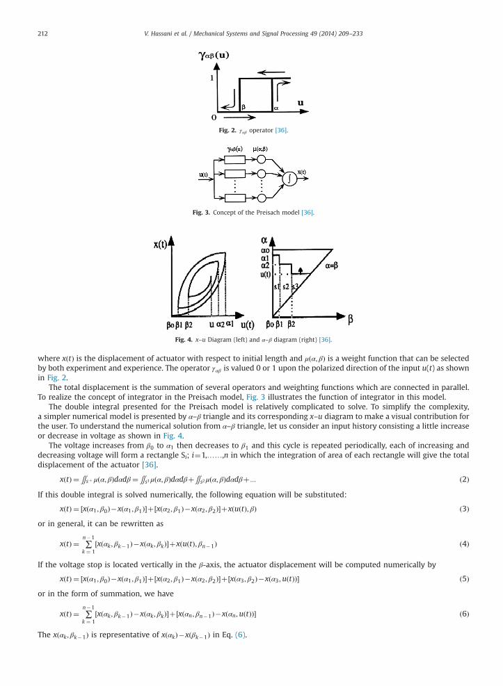
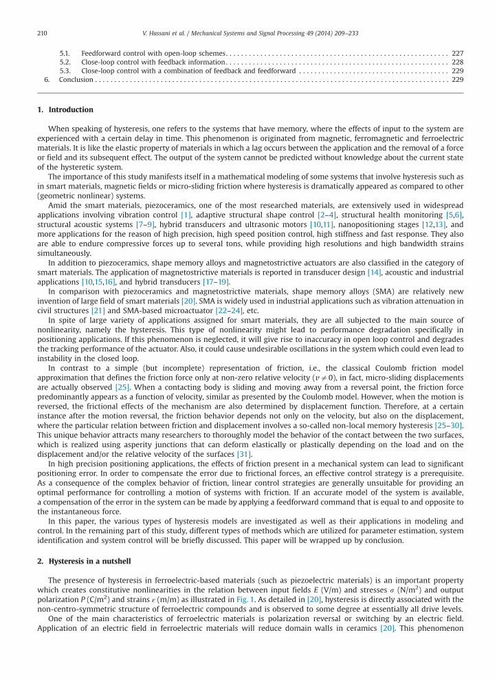
Fig. 2. γαβ operator [36].

Fig. 3. Concept of the Preisach model [36].

Fig. 4. x–u Diagram (left) and α–β diagram (right) [36].


where xðtÞ is the displacement of actuator with respect to initial length and μðα; βÞ is a weight function that can be selectedby both experiment and experience. The operator γαβ is valued 0 or 1 upon the polarized direction of the input u(t) as shownin Fig. 2.

The total displacement is the summation of several operators and weighting functions which are connected in parallel.To realize the concept of integrator in the Preisach model, Fig. 3 illustrates the function of integrator in this model.

The double integral presented for the Preisach model is relatively complicated to solve. To simplify the complexity,a simpler numerical model is presented by α–β triangle and its corresponding x–u diagram to make a visual contribution forthe user. To understand the numerical solution from α–β triangle, let us consider an input history consisting a little increaseor decrease in voltage as shown in Fig. 4.

The voltage increases from β0 to α1 then decreases to β1 and this cycle is repeated periodically, each of increasing anddecreasing voltage will form a rectangle Si; i¼1,……,n in which the integration of area of each rectangle will give the totaldisplacement of the actuator [36].

xðtÞ ¼∬sþ μðα; βÞdαdβ¼∬s1μðα; βÞdαdβþ∬s2μðα; βÞdαdβþ ::: ð2Þ

If this double integral is solved numerically, the following equation will be substituted:

xðtÞ ¼ ½xðα1; β0Þ�xðα1; β1Þ�þ½xðα2; β1Þ�xðα2; β2Þ�þxðuðtÞ; βÞ ð3Þor in general, it can be rewritten as

xðtÞ ¼ ∑n�1

k ¼ 1½xðαk; βk�1Þ�xðαk; βkÞ�þxðuðtÞ; βn�1Þ ð4Þ

If the voltage stop is located vertically in the β-axis, the actuator displacement will be computed numerically by

xðtÞ ¼ ½xðα1; β0Þ�xðα1; β1Þ�þ½xðα2; β1Þ�xðα2; β2Þ�þ½xðα3; β2Þ�xðα3;uðtÞÞ� ð5Þor in the form of summation, we have

xðtÞ ¼ ∑n�1

k ¼ 1½xðαk; βk�1Þ�xðαk; βkÞ�þ½xðαn; βn�1Þ�xðαn;uðtÞÞ� ð6Þ

The xðαk; βk�1Þ is representative of xðαkÞ�xðβk�1Þ in Eq. (6).

Table 1Construction of α–β triangle [39].

α (V) β (V)

0 30 60 90 120 150 180 210 240 270

300 19.98 19.40 18.25 16.29 13.72 10.76 7.95 5.46 3.33 1.54270 18.13 17.36 16.22 14.32 11.81 8.90 6.11 3.69 1.67240 15.75 14.98 13.85 11.97 9.50 6.66 3.96 1.78210 12.86 12.09 10.97 9.13 6.72 4.11 1.78180 9.69 8.92 7.80 5.96 3.78 1.59150 6.82 6.06 4.95 3.25 1.42120 4.34 3.60 2.54 1.2490 2.46 1.77 0.8560 1.22 0.5830 0.57

Preisach function: X(α,β) (mm).


The Preisach model is widely used in the modeling of hysteresis in smart materials. This model shows good performanceto characterize hysteresis satisfactorily at narrow-band frequency as well as no-load condition. The accuracy of the Preisachmodel is gradually deteriorated as the pre-loading force and input frequency to the actuator are increased [37].

To increase the accuracy of the Preisach model, the modified Preisach is proposed for an integrated piezo-drivencantilever beam under quasi-static condition [38]. In this case, the Preisach model is modified using the finer mesh triangleand weighting functions in order to estimate the hysteretic behavior of the structure more accurately. An example of datareduction to build triangle of the Preisach model is shown in Table 1.

In some approaches, a hybrid model can improve the performance of the Preisach model, e.g., the Preisach model is fusedinto a 3-layered neural network to overcome inherent disadvantages in the Preisach model which mainly arise from thenumber of data points to train the model [40]. Similarly, the prediction accuracy of the Preisach model is effectivelyimproved using a neural network in which the input vector is designed such that the network is applied in real-timeapplication [41]. In another type of hybrid model, the tabulated Everette function is used in terms of the Preisach model toreduce the number of data points required in the classical Preisach model [42].

The classical Preisach model is rate-independent; meanwhile, the model is not sensitive to variation of rate of inputapplied to the system. On the other hand, hysteresis is a rate-dependent phenomenon [36]. As a result, to achieve the rate-dependent Preisach model, some modifications are needed. To get the gist of it, these modifications have to change themodel such that it is used in dynamic applications. In this respect, a hysteresis operator first order differentialequation (HOFODE) can be replaced by the Preisach model [43]. Since the Preisach model is similar to the modifieddiagonal recurrent neural network (MDRNN) regarding the structural point of view, the proposed HOFODE is implementedusing the MDRNN.

As a substitute, a neural network can be used with the Preisach model such that the input vector of the network includesthe same input vector as utilized in the Preisach model in addition to the velocity of the actuator in order to predict thedisplacement output of the actuator over a wide range of frequency [36].

Dissimilar to [36,43] in which the Preisach model is replaced by neural network, a novel modified rate-dependentPreisach model is proposed based on the approximation of density function using the fast Fourier transform (FFT) [44].

The Preisach model can also be used in the control framework. The inverse of the Preisach model is used as feedforwardcompensator in a control loop. This compensator is normally used as a tool to mitigate the effect of hysteresis nonlinearity inmaterials. If the linear model of the actuator is approximated, the inverse of the Preisach model can be employed parallelwith any types of linear controllers such as PD/lead-lag compensator to improve the tracking performance of the controlsystem [45].

Similarly, the inverse of the modified Preisach model is used as feedforward controller with PID controller to improve theperformance of the linear PID controller [46] and also to control the joint angle of a manipulator driven by pneumaticartificial muscles [47].

The methodology proposed in [47] is pursued in [48] in which a linear–nonlinear system identification and control arecarried out using the composite approach which combines the nonlinear properties of the piezoelectric mechanism whichmainly arise from hysteresis in piezoelectric actuator and linear approximation of the mechanism regardless of nonlinearityin the system.

The dual integral in the Preisach mathematical model presents a big challenge to construct the inverse of the modeleasily. Using the inverse multiplicative technique enables us to split the Preisach model into non-memory and memoryparts. Thanks to this methodology, it is only sufficient to derive the inverse of the non-memory part to obtain an expressionfor the control input signal [49].

Alternatively, the Preisach model is used along with some nonlinear controllers, e.g., a neural network sliding modecontrol is fused to the Preisach model to control a system with unknown hysteresis. In this work, neural network is utilizedto predict the effect of hysteresis, while the sliding mode controller cancels the hysteresis effect on the system [50].


Atomic force microscopy is a method to measure the surface roughness and topology within the manufacturing process.If the piezoelectric scanning system is built accurate enough, the results of the scanning process will be more reliable.To measure the surface roughness precisely, an indirect adaptive controller is used as feedback controller to control themotion of the piezoelectric scanning system. In order to increase the accuracy of the system, the inverse of the Preisachmodel is used as feedforward controller with the indirect adaptive controller [51].

In an innovative control system design, a Preisach model is substituted by plant model of a shape memory alloy actuatorand cascaded with a PID controller. The error between the desired output and the output stemmed from the Preisach modelis feedback to PID controller. The parameters of the PID controller are optimized using the genetic algorithm to minimize acost function which is expressed in terms of sum of square of errors between the desired output and the output of thePreisach model [52]. Alternatively, the parameters of the PID controller are tuned by fuzzy logic rules in another design [53].

The combination of the LuGre friction model and the Preisach model enables us to characterize the hysteresis behavior inmaterials efficiently. Using the combined model, a back-stepping sliding mode control strategy is applied to seed the controlalgorithm and estimate the parameters of the controller by Lyapunov function, accordingly [54]. For detailed investigation ofthe control strategies designed for a system suffering from the hysteresis nonlinearity, readers may refer to Section 5.

Notwithstanding, the Preisach model is widely used for hysteresis characterization, it has some disadvantages that arelisted below [40]:

(1)
Total amount of data collected through the experiment will influence the accuracy of the Preisach model. (2) Since this model uses double integrator, constructing the inverse of the model is not easy. In result, it is not convenient
to use this model in real-time applications.
(3) True physics of the system cannot be implemented through this model.
As a result, the Krasnosel'skii–Pokrovskii (KP) model and Prandtl–Ishlinskii (PI) model are derived from the Preisachmodel to overcome the disadvantages existing in the Preisach model.

3.2. Krasnosel’skii–Pokrovskii (KP) model

After proposing the Preisach model by a German physicist F. Preisach, the Russian mathematician, Krasnosel’skii,introduced the Preisach model into a pure formalized mathematical form in which hysteresis is modeled by linearcombination of hysteresis operators [55].

Contrary to the operator used in the Preisach model that creates jump discontinuities in the model, the KP model allowsa great combination of functions to be replaced by the Preisach operators. The KP kernel, the elementary operator of the KPmodel which is a special case of generalized play operator, is a continuous function on the Preisach plane including minorloops within its major loop, where the Preisach plane is defined as

P ¼ fpðp1; p2ÞAℜ2:U� rp1rp2rUþ �ag ð7Þ

where Uþ and U� represent the positive and negative saturation values of input uðtÞAC½0; T � respectively. The positiveconstant value, a, is the rise constant of the kernel. Let C½0; T � denote the space of continuous piecewise monotone functionson the interval ½0; T�, then the elementary KP hysteresis operator is expressed as

Kpðu; ξpÞ:C½0; T �-y½0; T�

where ξp, parameterized by P, represents the initial condition of the kernel and the memory of the previous extreme outputof the kernel, and y½0; T � is the output space. For a specific amount of uðtÞ, the KP operator Kpðu; ξpÞ maps points pðp1; p2Þ tothe interval ½�1;1� and is given by

Kpðu; ξpÞðtÞ ¼max fξp; rðuðtÞ�p2Þg _uðtÞ40min fξp; rðuðtÞ�p1Þg _uðtÞo0

(ð8Þ

where rð:Þ is the Lipschitz continuous ridge function. The ridge function can be expressed in any form but it is popular to beselected in terms of a continuous piecewise linear function defined as

rðxÞ ¼�1 xo0�1þ2x

a 0rxra

þ1 x40

8><>: ð9Þ

Using the above equations, the KP operator is illustrated in Fig. 5. By comparing the Preisach operator, it is evidentlyobserved that the KP operator consists of family of curves that are bounded by the curves rðu�p2Þ and rðu�p1Þ between theenvelop ranging from p1 to p2þa.

The KP hysteresis output is expressed using the double integral as follows:

yðtÞ ¼∬pkpðuðtÞ; ξpÞμðp1; p2Þdp1dp2 ð10Þ

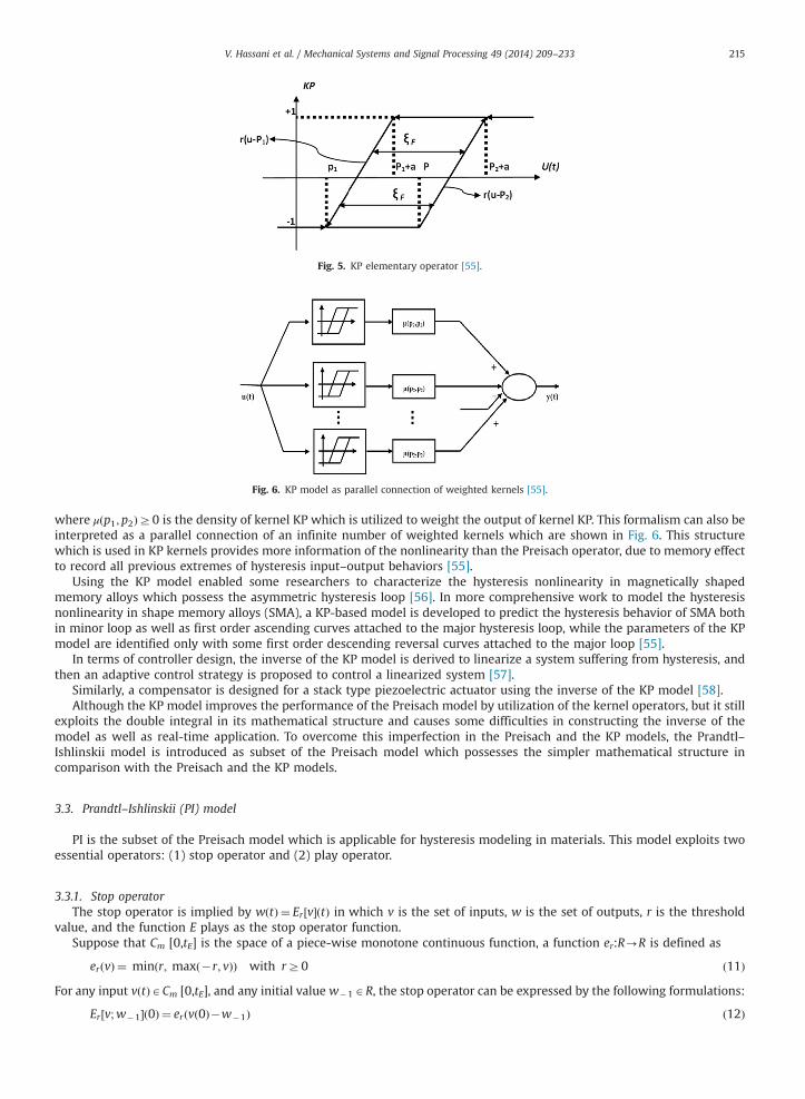
Fig. 5. KP elementary operator [55].

Fig. 6. KP model as parallel connection of weighted kernels [55].


where μðp1; p2ÞZ0 is the density of kernel KP which is utilized to weight the output of kernel KP. This formalism can also beinterpreted as a parallel connection of an infinite number of weighted kernels which are shown in Fig. 6. This structurewhich is used in KP kernels provides more information of the nonlinearity than the Preisach operator, due to memory effectto record all previous extremes of hysteresis input–output behaviors [55].

Using the KP model enabled some researchers to characterize the hysteresis nonlinearity in magnetically shapedmemory alloys which possess the asymmetric hysteresis loop [56]. In more comprehensive work to model the hysteresisnonlinearity in shape memory alloys (SMA), a KP-based model is developed to predict the hysteresis behavior of SMA bothin minor loop as well as first order ascending curves attached to the major hysteresis loop, while the parameters of the KPmodel are identified only with some first order descending reversal curves attached to the major loop [55].

In terms of controller design, the inverse of the KP model is derived to linearize a system suffering from hysteresis, andthen an adaptive control strategy is proposed to control a linearized system [57].

Similarly, a compensator is designed for a stack type piezoelectric actuator using the inverse of the KP model [58].Although the KP model improves the performance of the Preisach model by utilization of the kernel operators, but it still

exploits the double integral in its mathematical structure and causes some difficulties in constructing the inverse of themodel as well as real-time application. To overcome this imperfection in the Preisach and the KP models, the Prandtl–Ishlinskii model is introduced as subset of the Preisach model which possesses the simpler mathematical structure incomparison with the Preisach and the KP models.

3.3. Prandtl–Ishlinskii (PI) model

PI is the subset of the Preisach model which is applicable for hysteresis modeling in materials. This model exploits twoessential operators: (1) stop operator and (2) play operator.

3.3.1. Stop operatorThe stop operator is implied by wðtÞ ¼ Er ½v�ðtÞ in which v is the set of inputs, w is the set of outputs, r is the threshold

value, and the function E plays as the stop operator function.Suppose that Cm [0,tE] is the space of a piece-wise monotone continuous function, a function er:R-R is defined as

erðvÞ ¼ minðr; maxð�r; vÞÞ with rZ0 ð11Þ

For any input vðtÞACm [0,tE], and any initial value w�1AR, the stop operator can be expressed by the following formulations:

Er ½v;w�1�ð0Þ ¼ erðvð0Þ�w�1Þ ð12Þ

Fig. 7. Hysteresis operators: (a) stop operator and (b) play operator [60].


Er½v;w�1�ðtÞ ¼ erðvðtÞ�vðtiÞþEr ½v;w�1�ðtiÞÞtiotrtiþ1 and 0r irN�1 ð13Þ

It is also assumed that the function v is monotone on each of the sub-intervals [ti,tiþ1]. This operator basically determinesthe height of the hysteresis region in the input–output or ðv;wÞ plane [59]. This operator can be seen in Fig. 7(a).

3.3.2. Play operatorPlay operator is a continuous and rate-independent operator. In this operator, repeatedly, suppose Cm [0,tE] represents

the space of piecewise monotone continuous function. The function v is monotone on [0,tE] and each of the sub-intervals[ti,tiþ1].

The operator is defined by

Fr½v�ð0Þ ¼ f rðvð0Þ;0Þ ¼wð0Þ ð14Þ

Fr½v�ðtÞ ¼ f rðvðtÞ; Fr½v�ðtiÞÞ; for tiotrtiþ1 and 0r irN�1 ð15Þwhere

f rðv;wÞ ¼ maxðv�r; minðvþr;wÞÞ ð16ÞThe relation between the stop operator and the play operator is expressed as

Er½v;w�1�ðtÞþFr ½v;w�1�ðtÞ ¼ vðtÞ ð17ÞBasically, two main elements of the play operator are the input v and the threshold value r [59]. The play operator is shownin Fig. 7(b).

In a continuous format of the play operator, the hysteresis relationship between the output, y, and the input, v, can berepresented by the following integral:

yp ¼ qvðtÞþZ R

0pðrÞFr ½v�ðtÞdr ð18Þ

where p(r)Z0 is a density function which is usually identified by experimental data and q is a constant. For the reason ofconvenience, the value, R is assumed R¼1 in the literatures. For further understanding of the operators applied in the PImodel, reader may refer to the procedure of the simulation in MATLAB Simulink presented in [61]. In [62], a modified PI isproposed in terms of the right-hand and the left-hand play operators to model the multi-loop ascending and descendinghysteresis loops.

In practice, depending on the input magnitude and the input frequency applied to the actuator, the hysteresis loop showsdifferent behaviors. One of these behaviors appears as an asymmetric hysteresis loop. The generalized rate-independent PIis proposed to overcome the imperfections that we face in modeling the asymmetric hysteresis loops with the classical PI.The only change made in the classical model to transform it to the generalized one is attributed to the threshold value.Two envelop functions as γl and γr are defined instead of the threshold value, r, in the classical model that are subsequentlyrepresented for left and right envelops of the hysteresis curve [63]. Regarding the shape of the hysteresis curve, differentmathematical functions such as linear, tangent hyperbolic, etc. can be used as envelop function. The generalized PI model is

Fig. 8. Generalized play operator [63].


expressed for the play operator as

Fγlr ½v�ð0Þ ¼ f γlr ðvð0Þ;0Þ ¼wð0Þ ð19Þ

Fγlr ½v�ðtÞ ¼ f γlr ðvðtÞ; Fγlr½v�ðtiÞÞ; ð20Þ

For tiotrtiþ1 and 0r irN�1

f γlr ðv;wÞ ¼ maxðγlðvÞ�r; minðγrðvÞþr;wÞÞ ð21Þ

and for the stop operator, we have

Eγlr ½v;w�1�ð0Þ ¼ eγlr ðvð0Þ�w�1Þ ð22Þ

Eγlr ½v;w�1�ðtÞ ¼ eγlr ðvðtÞ�vðtiÞþEγlr ½v;w�1�ðtiÞÞ; ð23Þ

For tiotrtiþ1 and 0r irN�1

eγlrðvÞ ¼ minðγlðvÞþr; maxðγrðvÞ�r; vÞÞ ð24ÞFig. 8 shows an example of asymmetric hysteresis loop and the respective envelop functions for ascending and

descending hysteresis curves [63].A different approach is used to model the asymmetric hysteresis loop occurring in piezoelectric actuator utilized for

atomic force microscopy imaging. In this approach, as an alternative approach to [63] at which envelop functions areproposed for ascending and descending loops, different slope values describe the forward and backward hysteresisloops [64].

As described earlier in Section 3.1, the hysteresis phenomenon apparently appears as a function of frequency. Meanwhile,by increasing or decreasing the input rate or input frequency, the intensity of the hysteresis will increase or decreaseconsequently. Due to this property, different PI models are proposed in terms of rate-dependent model. In [60,65,66], a newmathematical model is proposed with a logarithmic threshold function in the play operator of the classical PI model whichis the function of the input rate applied to the actuator. This function is written as

r¼ α ∏z

l ¼ 1ln ðβlþλlj_vðtÞjεÞ ð25Þ

where α and λl are the positive constants, βlZ1, εZ1 and z determines the number of operators in a particular problem,whereas _vðtÞ stands for the rate of input applied to the material. Based on this definition, the output of the rate-dependentplay operator is obtained by means of the following formulation:

ypðkÞ ¼wkvkþ ∑Q

k ¼ 1gkpkFrk ð26Þ

where wk and gk depend on the nature of hysteresis and the type of material used in the actuator. These values can beselected either as constant quantities or in terms of mathematical expression as

wðv; _vÞ ¼ a1e�m1 _vem2v ð27Þ

gðv; _vÞ ¼ a2e� s1 _ves2v ð28Þwhere a140 and a240, m1; m2; s1 and s2 are constants to be determined by experimental data. Frk is the play operator asgiven in Eqs. (15) and (16). On the contrary, the threshold value rk is a function of input frequency. In the following model,a generalized rate-dependent PI is designed to capture the asymmetric hysteresis curve at relatively wide range of frequencybetween 0 and 200 Hz [65].


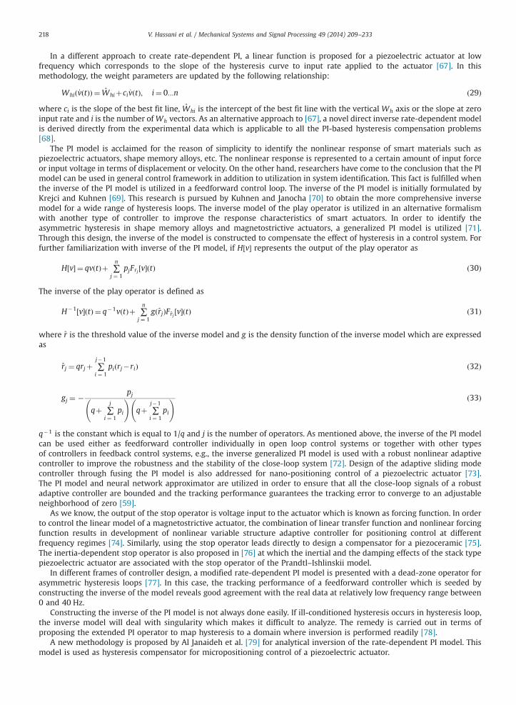
In a different approach to create rate-dependent PI, a linear function is proposed for a piezoelectric actuator at lowfrequency which corresponds to the slope of the hysteresis curve to input rate applied to the actuator [67]. In thismethodology, the weight parameters are updated by the following relationship:

Whið_vðtÞÞ ¼ Whiþci _vðtÞ; i¼ 0:::n ð29Þ

where ci is the slope of the best fit line, Whi is the intercept of the best fit line with the vertical Wh axis or the slope at zeroinput rate and i is the number ofWh vectors. As an alternative approach to [67], a novel direct inverse rate-dependent modelis derived directly from the experimental data which is applicable to all the PI-based hysteresis compensation problems[68].

The PI model is acclaimed for the reason of simplicity to identify the nonlinear response of smart materials such aspiezoelectric actuators, shape memory alloys, etc. The nonlinear response is represented to a certain amount of input forceor input voltage in terms of displacement or velocity. On the other hand, researchers have come to the conclusion that the PImodel can be used in general control framework in addition to utilization in system identification. This fact is fulfilled whenthe inverse of the PI model is utilized in a feedforward control loop. The inverse of the PI model is initially formulated byKrejci and Kuhnen [69]. This research is pursued by Kuhnen and Janocha [70] to obtain the more comprehensive inversemodel for a wide range of hysteresis loops. The inverse model of the play operator is utilized in an alternative formalismwith another type of controller to improve the response characteristics of smart actuators. In order to identify theasymmetric hysteresis in shape memory alloys and magnetostrictive actuators, a generalized PI model is utilized [71].Through this design, the inverse of the model is constructed to compensate the effect of hysteresis in a control system. Forfurther familiarization with inverse of the PI model, if H½v� represents the output of the play operator as

H½v� ¼ qvðtÞþ ∑n

j ¼ 1pjFrj ½v�ðtÞ ð30Þ

The inverse of the play operator is defined as

H�1½v�ðtÞ ¼ q�1vðtÞþ ∑n

j ¼ 1gðrjÞFrj ½v�ðtÞ ð31Þ

where r is the threshold value of the inverse model and g is the density function of the inverse model which are expressedas

rj ¼ qrjþ ∑j�1

i ¼ 1piðrj�riÞ ð32Þ

gj ¼ � pj

qþ ∑j

i ¼ 1pi

!qþ ∑

j�1

i ¼ 1pi

! ð33Þ

q�1 is the constant which is equal to 1/q and j is the number of operators. As mentioned above, the inverse of the PI modelcan be used either as feedforward controller individually in open loop control systems or together with other typesof controllers in feedback control systems, e.g., the inverse generalized PI model is used with a robust nonlinear adaptivecontroller to improve the robustness and the stability of the close-loop system [72]. Design of the adaptive sliding modecontroller through fusing the PI model is also addressed for nano-positioning control of a piezoelectric actuator [73].The PI model and neural network approximator are utilized in order to ensure that all the close-loop signals of a robustadaptive controller are bounded and the tracking performance guarantees the tracking error to converge to an adjustableneighborhood of zero [59].

As we know, the output of the stop operator is voltage input to the actuator which is known as forcing function. In orderto control the linear model of a magnetostrictive actuator, the combination of linear transfer function and nonlinear forcingfunction results in development of nonlinear variable structure adaptive controller for positioning control at differentfrequency regimes [74]. Similarly, using the stop operator leads directly to design a compensator for a piezoceramic [75].The inertia-dependent stop operator is also proposed in [76] at which the inertial and the damping effects of the stack typepiezoelectric actuator are associated with the stop operator of the Prandtl–Ishlinskii model.

In different frames of controller design, a modified rate-dependent PI model is presented with a dead-zone operator forasymmetric hysteresis loops [77]. In this case, the tracking performance of a feedforward controller which is seeded byconstructing the inverse of the model reveals good agreement with the real data at relatively low frequency range between0 and 40 Hz.

Constructing the inverse of the PI model is not always done easily. If ill-conditioned hysteresis occurs in hysteresis loop,the inverse model will deal with singularity which makes it difficult to analyze. The remedy is carried out in terms ofproposing the extended PI operator to map hysteresis to a domain where inversion is performed readily [78].

A new methodology is proposed by Al Janaideh et al. [79] for analytical inversion of the rate-dependent PI model. Thismodel is used as hysteresis compensator for micropositioning control of a piezoelectric actuator.


3.4. Maxwell-Slip model

This model is basically a tool to express hysteresis nonlinearity in both mechanical and electrical systems. Originally, thismodel was proposed to show the behavior of friction in mechanical systems. The function of this model is similar to the stopoperator in the PI model.

This model operates with an elasto-slide element comprising of a massless linear spring and a massless block which aresusceptible to Coulomb friction, F. The relationship for this element is described by

F ¼kðx�xbÞ kðx�xbÞ

�� o f

f sgnð_xÞ xb ¼ x� fksgnð_xÞ

8<: ð34Þ

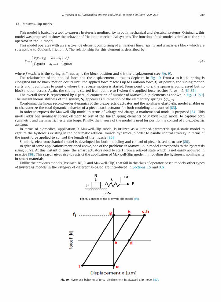
where f ¼ μ:N, k is the spring stiffness, xb is the block position and x is the displacement (see Fig. 9).The relationship of the applied force and the displacement output is depicted in Fig. 10. From a to b, the spring is

elongated but no block motion occurs until the applied force reaches up to Coulomb force, fi. At point b, the sliding motionstarts and it continues to point c where the reverse motion is started. From point c to e, the spring is compressed but noblock motion occurs. Again, the sliding is started from point e to f when the applied force reaches force �fi [81,82].

The overall force is represented by a parallel connection of number of Maxwell-Slip elements as shown in Fig. 11 [80].The instantaneous stiffness of the system, Sj, appears as summation of the elementary springs, ∑n

i ¼ jki.Combining the linear second-order dynamics of the piezoelectric actuator and the nonlinear elasto-slip model enables us

to characterize the total dynamic behavior of a piezo-stack actuator for both modeling and control [83].In order to express the Maxwell-Slip model in terms of voltage and charge, a mathematical model is proposed [84]. This

model adds one nonlinear spring element to rest of the linear spring elements of Maxwell-Slip model to capture bothsymmetric and asymmetric hysteresis loops. Finally, the inverse of the model is used for positioning control of a piezoelectricactuator.

In terms of biomedical application, a Maxwell-Slip model is utilized as a lumped-parametric quasi-static model tocapture the hysteresis existing in the pneumatic artificial muscle dynamics in order to handle control strategy in terms ofthe input force applied to control the length of the muscle [85].

Similarly, electromechanical model is developed for both modeling and control of piezo-based structure [80].In spite of some applications mentioned above, one of the problems in Maxwell-Slip model corresponds to the hysteresis

rising curve. At this instant of time, the smart actuators need to start from a relaxed state which is not easily acquired inpractice [86]. This reason gives rise to restrict the application of Maxwell-Slip model in modeling the hysteresis nonlinearityin smart materials.

Unlike the previous models (Preisach, KP, PI and Maxwell-Slip) that fall in the class of operator-based models, other typesof hysteresis models in the category of differential-based are introduced in Sections 3.5 and 3.6.

Fig. 9. Concept of the Maxwell-Slip model [80].

Fig. 10. Hysteresis behavior of force–displacement in Maxwell-Slip model [80].

Fig. 11. Multiple elasto-slide elements (left) and multiple elasto-slide elements behavior (right) [80].


3.5. Bouc–Wen model

In general, the Bouc–Wen model is expressed by means of a nonlinear differential equation as follows:

_z¼ A _u�βj _ujzjzjn�1�γ _ujzjn ð35Þwhere the parameters A, β and γ determine the shape of hysteresis and n is an integer number. Z in this equation is a statevariable which is integrated by the state-space equations of the system and _u is the derivative of existing input [87].

In this context, one can find myriad of proposed models in modeling and control of hysteresis. To model the hysteresisnonlinearity in a large scale magnetorheological damper, an innovative identification model is used to estimate theparameters of a Bouc–Wen model [88].

To transform the Bouc–Wen model into a rate-dependent one, this model is formulated together with a linearHammerstein model in which the former one models the static hysteresis in a piezoelectric actuator while the latter is usedto model the rate-dependent hysteresis in a relatively low range frequency from 1 Hz to 100 Hz [89].

The Bouc–Wen model can also be applied with different types of controllers, e.g., in one design, three control laws aredefined in terms of PID controller for micro-positioning control of a piezoelectric actuator modeled by the Bouc–Wenhysteresis model [90]. The PID controller with time-varying parameter shows the best tracking performance among theothers.

To evaluate the combination of fuzzy T–S model and the genetic algorithm in control system design, the linearization ofthe Bouc–Wen model is carried out by T–S fuzzy rule and the parameters of the model are estimated by genetic algorithm[91]. In the last part of controller design, an LMI-based controller is designed to stabilize the system in an optimal manner.

Alternatively, a fuzzy-based PD controller is used for a piezoelectric actuator which is dynamically modeled by the Bouc–Wen hysteresis model [92]. Simulation results reveal that the controller is robust against external disturbances.

In order to improve the performance of nonlinear system, a back-stepping nonlinear control is proposed for a piezo-based structure [93]. In this design, first of all, the Bouc–Wen model is established for modeling the hysteresis in actuator,then the back-stepping controller is designed based on the parameters of the model. Finally, the performance of the back-stepping controller is compared with a linear PID controller. In the area of nonlinear control, repeatedly, a model referenceadaptive nonlinear controller is designed to control a piezoelectric moving element [94].

Since the Bouc–Wen model is not invertible, a Bouc–Wen least square support vector machine (LSSVM) is designedeither to identify or compensate hysteresis in feedforward path without the need to model hysteresis inverse [95]. In otherresearch, a multiplicative-inverse structure approach is proposed to design a compensator for the hysteresis nonlinearity inthe piezoelectric actuator which is expressed by the Bouc–Wen model [96]. This strategy allows us that no morecomputation is carried out for the compensator as well as adaptation with the Bouc–Wen model.

3.6. Duhem model

This model is another type of differential-based hysteresis model which is presented in a more complex way than theBouc–Wen model. This model was proposed in 1897 to simulate an active hysteresis. The design was based on the approachthat the output (w) can change its characteristics when the input (v) changes its direction [97]. To express it into amathematical form, suppose we have

dwdt

¼ αdvdt

�� f ðvÞ�w� �þdv

dtgðvÞ ð36Þ

where α is constant and positive.


This model is fulfilled, if the following conditions are satisfied:

Condition 1: f (.) is piecewise smooth, monotone increasing, odd, with limv-1

f 0ðvÞ finite.Condition 2: g (.) is piecewise continuous, even, with lim

v-1gðvÞ ¼ lim

v-1f 0ðvÞ.

Condition 3: f 0ðvÞ4gðvÞ4αeαvR1v f 0ðξÞ�gðξÞ�� e�αξdξ for all v40.

The differential Duhem model is solved:

w¼ f ðvÞþ½w0� f ðv0Þ�e�αðv�v0Þsgnð_vÞþe�αvsgnð_vÞZ v

v0½gðξÞ� f 0ðξÞ�eαξsgnð_vÞdξ ð37Þ

and the above solution can be simplified by

w¼ f ðvÞþφðvÞ ð38ÞAscending wl belongs to a time sgnð_vÞ ¼ 1 and the solution changes to

wlðvÞ ¼ f ðvÞþ½w0� f ðv0Þ�e�αðv�v0Þ �e�αvZ v

v0½f 0ðξÞ�gðξÞ�eαξdξ vZv0 ð39Þ

and the descending wu is when the sgnð_vÞ ¼ �1 and the new solution is

wuðvÞ ¼ f ðvÞþ½w0� f ðv0Þ�e�αðv0 �vÞ �e�αvZ v0

v½f 0ðξÞ�gðξÞ�eαξdξ vrv0 ð40Þ

As can be seen from both the relationships for wu and wl, when v is going to 1 or �1 the condition 2 is satisfied [97]

limv-1

½wlðv; v0;w0Þ� f ðvÞ� ¼ 0 ð41Þ

limv-�1

½wuðv; v0;w0Þ� f ðvÞ� ¼ 0 ð42Þ

The Duhem model is rate-independent. The big challenge in this model is to find out f ðvÞ and gðvÞ which are functions ofinput voltage influencing on both the model performance and the hysteresis loop [86]. In order to approximate thesefunctions, in one research, a polynomial is proposed based on the well-known Weierstrass theorem [98]. Finally, thecoefficients of these polynomials are estimated using the recursive least squares method.

The Coleman–Hodgdon model, special case of the Duhem model, is used to model unknown hysteresis nonlinearity in asystem [99]. Consequently, in this work, a robust sliding mode control scheme is proposed to mitigate the effect of hysteresisusing the Coleman–Hodgdon model without any need of constructing the inverse of the model.

Similarly, the Duhem model can be fused to a robust control law in order to achieve the desired precision in trackingperformance [97]. As said earlier, since the Duhem model is a differential-based model, construction of the inverse is adifficult task. This fact motivated Feng et al. [97] to present an adaptive nonlinear controller based on the Duhem model toensure the stability of the system globally in spite of unknown hysteresis existing in the system.

Based on the system identification performed for a giant magnetostrictive actuator (GMA), a combination of linear–nonlinear model is obtained to model the dynamic characteristics of GMA. Using this model, a robust sliding modecontroller is designed to improve the tracking performance as compared to linear controllers [100].

In addition to hysteresis models discussed in Sections 3.1–3.6, reader may refer to some works done with othermathematical models for hysteresis characterization in materials [101–103].

4. System identification strategies in hysteresis characterization

Most of the models considered in the previous section consist of many parameters to build the shape of the hysteresiscurve. In the first place, a suitable model has to be assigned to describe a nonlinear behavior of the system properly, andthen the parameters of the proposed model have to be estimated. This matter can be considered from two different points ofviews. In one hand, an identifier can be designed and substituted to the model of the system for imitating the behavior ofthe real system as nearly as possible with a minimum error. This kind of identification is known as non-parametricidentification. On the other hand, parameters of the proposed model can be estimated through an optimization tools.This type of identification is known as parametric identification in which the parameters of the system are estimated usingseveral methods such as least mean square, recursive least square, genetic algorithm, particle swarm optimization, etc.

4.1. Least mean square-based system identification

Within this discipline, the model is often presented in a regression form, afterward, the parameters of the regressionmodel will be estimated through the least mean square method on the input and output data sets which are taken from anexperiment or simulation. The mechanism of this methodology is shown in Fig. 12.

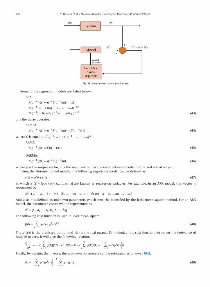
Fig. 12. Least mean square mechanism.


Some of the regression models are listed below:

ARX:

Aðq�1ÞyðtÞ ¼ q�dBðq�1ÞuðtÞþεðtÞAðq�1Þ ¼ 1þa1q�1þ :::::::þanaq�na

Bðq�1Þ ¼ b0þb1q�1þ ::::::þbnbq�nb ð43Þ

q is the delay operator.

ARMAX:

Aðq�1ÞyðtÞ ¼ q�dBðq�1ÞuðtÞþCðq�1ÞεðtÞ ð44Þwhere C is equal to Cðq�1Þ ¼ 1þc1q�1þ ::::::þcncqnc

ARMA:

Aðq�1ÞyðtÞ ¼ Cðq�1ÞεðtÞ ð45Þ

DARMA:

Aðq�1ÞyðtÞ ¼ q�dBðq�1ÞuðtÞ ð46Þwhere y is the output vector, u is the input vector, ε is the error between model output and actual output.

Using the aforementioned models, the following regression model can be defined as:

yðtÞ ¼ φTθþeðtÞ ð47Þin which φT ðtÞ ¼ ½φ1ðtÞ;φ2ðtÞ; :::::::;φnðtÞ� are known as regression variables. For example, in an ARX model, this vector isrecognized by

φT ðtÞ ¼ ½�yðt�1Þ; �yðt�2Þ; :::; �yðt�nÞ;uðt�dÞ;uðt�d�1Þ; :::;uðt�d�mÞ�And also, θ is defined as unknown parameters which must be identified by the least mean square method. For an ARXmodel, the parameter vector will be represented as

θT ¼ ½a1; a2; :::; an; b0;b1; :::; bn�The following cost function is used in least mean square:

JðθÞ ¼ ∑N

t ¼ 1½yðtÞ�φT ðtÞθ�2 ð48Þ

The φT ðtÞθ is the predicted output and y(t) is the real output. To minimize this cost function, let us set the derivative of∂JðθÞ=∂θ to zero, it will give the following relation:

∂JðθÞ∂θ

¼ �2 ∑N

t ¼ 1φðtÞ½yðtÞ�φT ðtÞθ� ¼ 0 ) ∑

N

t ¼ 1φðtÞyðtÞ ¼ ∑

N

t ¼ 1φðtÞφT ðtÞ

� �θ

Finally, by making the inverse, the unknown parameters can be estimated as follows [104]:

θN ¼ ∑N


� ��1

∑N

t ¼ 1φðtÞyðtÞ ð49Þ


Regarding system identification by the least mean square method, a bivariate probability density function (pdf) is used interms of the Preisach model to capture hysteresis in shape memory alloys and ferromagnetic materials [105].

An adaptive inverse model approach is also used for micropositioning control of a piezoelectric actuator in which thehysteresis is mathematically modeled and the parameters of the model are updated by least mean square algorithm [106].

4.2. Recursive least square-based system identification

This method is a tool to estimate unknown parameters of a system in a dynamic manner. This method is the extendedtype of least mean square algorithm.

At the beginning of this algorithm, let us assume,

∑N


� �¼ RðtÞ ð50Þ

∑N

t ¼ 1φðtÞyðtÞ

� �¼ f ðtÞ ð51Þ

Then we have

θt ¼ R�1ðtÞf ðtÞ ð52Þ

where RðtÞ and f ðtÞ can be written in time-dependent terms as

RðtÞ ¼ λðtÞRðt�1ÞþφðtÞφT ðtÞ ð53Þ

f ðtÞ ¼ λðtÞf ðt�1ÞþφðtÞyðtÞ ð54Þ0oλðtÞo1 is the forgetting factor that will exponentially give less weight to earlier samples. By substituting (54) into (52),we have

RðtÞ ¼ λðtÞRðt�1ÞþφðtÞφT ðtÞ ð55Þ

θðtÞ ¼ θðt�1ÞþR�1ðtÞφðtÞ½yðtÞ�φT ðtÞθðt�1Þ� ð56Þ

Calculating the inverse of RðtÞ is the time consuming process. To overcome this problem, the matrix inverse lemma is used toeliminate R

�1from (56). By utilizing this lemma, the recursive least square rule changes into the following form:

θðtÞ ¼ θðt�1Þþ pðt�1ÞφðtÞλðtÞþφT ðtÞpðt�1ÞφðtÞ yðtÞ�φT ðtÞθðt�1Þ

h ið57Þ

pðtÞ ¼ 1λðtÞ pðt�1Þ�pðt�1ÞφðtÞφT ðtÞpðt�1Þ

λðtÞþφT ðtÞpðt�1ÞφðtÞ

� �ð58Þ

φ is the regression variable vector and θ is the parameter vector. P(t) is initialized by a large number in a positive definitematrix. These relationships show the time-dependent version of the least mean square algorithm that makes it adaptive andusable in on-line parameter estimation [104].

The hysteresis in piezoelectric actuators can be characterized using NMAX and NARMAX models [107]. The parameters ofthese models are estimated by the recursive least square method.

In another example of application of this methodology in parameter estimation, the dynamic equations of the impactdrive mechanism including two masses and one piezoelectric element are implemented together with the hysteresis modelof the piezoelectric actuator using the Bouc–Wen model [87]. After identification of the parameters by the adaptiverecursive least square method, the inverse of the model is used as feedforward controller to alleviate the effect of hysteresisin the impact drive mechanism.

4.3. Genetic algorithm-based system identification

This algorithm is used as a heuristic method of optimization in a category of random search methods. In thismethodology, parameters underlying estimation process are considered as chromosomes that form a string called gene asshown in Fig. 13. A certain amount of chromosomes are forming the population [108].

At the beginning of the algorithm, a fitness function is defined. The values of the initial chromosomes are selectedrandomly to form a population. The fitness function is calculated for each set of the chromosome and the algorithm ispreceded through iterations till the fitness function reaches out the best value. Upon the optimization process, i.e.,minimization or maximization, some steps of this algorithm can be briefly summarized as follows:

(1)
initialize the first population; (2) evaluate fitness function;

Fig. 13. Gene and chromosome in genetic algorithm [108].

Fig. 14. Conventional genetic algorithm flow chart.


(3)
select chromosomes; (4) perform crossover; (5) perform mutation; (6) report best chromosome as solution; and (7) go to step 2 for the next generation or iteration.
Fig. 14 shows the summary of the conventional genetic algorithm.In one research, three fitness functions are defined for estimation of the parameters of the Bouc–Wen model [109–111].

Kwok et al. [112] proposed an asymmetric Bouc–Wen model for characterization of hysteresis in a magnetorheological fluiddamper. A novel genetic algorithm with adaptive crossover and mutation stage is developed to optimize the parameters ofthe model.

A dual-stage X–Y positioned which is operated by permanent magnet for course displacement and two piezoelectricelements for fine displacement is dynamically modeled [113]. The hysteresis nonlinearity in piezoelectric actuator ismodeled by the Bouc–Wen model and the parameters of the model are identified by real-coded genetic algorithm. In aninnovative research, the hysteresis nonlinearity is approximated in the blood vessels using the Maxwell-Slip model [114].In this work, a new optimization strategy is opted to estimate the parameters of the model in terms of new geneticalgorithm approach which exploits locally crossover with pressure selection for variable length genotype.

4.4. System identification by particle swarm optimization (PSO)

Over the past decade, many types of optimization methods have been developed and used in many applicationsspecifically in identification, control, etc. The particle swarm optimization has been recently considered as a highperformance optimization tool that is very easy to understand and implement. It is known as an alternative method to


genetic algorithm. The idea is originated from the swarm movements of some groups of animals like bird flocking, fishschooling and swarm theory [115]. Owing to the genetic algorithm formalism, PSO has some advantages that makes it easyto implement and also has a memory for good solutions. In genetic algorithm, the previous knowledge of the problem isdestroyed once the population changes. Unlike genetic algorithm, each individual so-called the particle and each particleupdates its velocity towards its Pbest and gbest locations. “Pbest” is the best value for each agent and “gbest” is the best valuefor the agent in the group among Pbest [115].

The procedure of PSO is described as follows:

(1)
Initialize the time to zero and set a number for initial position xjð0Þ and initial velocity vjð0Þ. (2) Evaluate the fitness of each particle FðxjðtÞÞ. (3) Set the Pbestj(t) to the better performance via
PbestjðtÞ ¼Pbestjðt�1Þ FðxjðtÞÞZFðPbestjðt�1ÞxjðtÞ FðxjðtÞÞoFðPbestjðt�1Þ

(ð59Þ

(4)
Set the gbest(t) to the position of article with the best fitness within the swarm as
gbestðtÞAfPbest1ðtÞ; Pbest2ðtÞ; :::; PbestNS ðtÞg=FðgbestðtÞÞ ¼ min fFðPbest1ðtÞÞ; ::::; FðPbestNs ðtÞÞg ð60Þ

(5)
Update the velocity vector for each particle according to both equations and the following rule:
vjðtþ1Þ ¼Vmax vjðtþ1Þ4Vmax

�Vmax vjðtþ1Þo�Vmax

vjðtþ1Þ else

8><>: ð61Þ

Vmax is usually selected to be half of the length of the search space.
(6) Update the position of each particle according to its equation. (7) Update the inertial weight. (8) Let t¼tþ1. (9) Compute the new FðxjðtÞÞ until the iteration to be terminated or the least value for F to be achieved.
Ye and Wang [116] utilized improved particle swarm optimization (IPSO) combined with chaotic map to identify theparameters of the Bouc–Wen model proposed as hysteresis model for a system. Alternatively, the modified particle swarmoptimization (MPSO) is used to identify the parameters of Scott–Russell mechanism which is driven by a piezoelectricelement [114,115].

4.5. System identification by neural network

Neural network is one of the most powerful methods in system identification. It plays a role as a block box to substituteas a model of a plant. As mentioned earlier, the system identification is accomplished in two forms of parametric and non-parametric regimes. Most of the modeling performed by neural network is based on non-parametric identification;meanwhile, neural network is applied as a block box instead of a physical model of the system.

The dynamic neural network usually appears in the form of recurrent network (the network in which the output incurrent time is dependent to the output and the input of previous time (s)) to identify the behavior of a plant.

To apply neural network in hysteresis characterization, Dang and Tan [43] proposed a modified recurrent neural networkwhich is replaced by the Preisach model for a piezoelectric actuator. This network covers a certain range of frequency tocreate more adaptive model to variation of frequency. This network is trained by set of input and output at wide range offrequency. For further understanding, the summary of the training procedure is rewritten as follows:Output of the neuralnetwork is given by

yðkÞ ¼ ∑n

j ¼ 1w3

j HjðkÞ ð62Þ

where w3 is the output weight and HðkÞ is the hidden layer neurons, and n is the number of hidden layer. Hidden layer iscomputed as

HjðkÞ ¼ f ðsjðkÞÞ ð63Þ

where f is the activation function and s is calculated by the following relationship:

sjðkÞ ¼ ð1�αÞw22Hðk�1Þþα ∑n

j ¼ 1w1

j xðkÞ ð64Þ


α is an adjustable factor and its value varies between 0 and 1, w22 is the recurrent weight and xðkÞ is the input vector ofnetwork.

This network is trained (the weights are updated) by using the following cost function:

E¼ 12ðyrðkÞ�yðkÞÞ2 ¼ 1

2e2ðkÞ ð65Þ

yr is the desired output and y(k) is the neural network output.The training process is followed by tracking the following derivatives in terms of steepest descent gradient method

which is used for updating the weights and biases of the network.

∂E∂w3 ¼ �eHjðkÞ ð66Þ

∂E∂w22 ¼ �ew3f 0ðsjðkÞÞPjðkÞ ð67Þ

∂E∂w1 ¼ �ew3f 0ðsjðkÞÞQjðkÞ ð68Þ

PjðkÞ ¼∂SjðkÞ∂w22 ¼ ð1�αÞHjðk�1Þ; Pjð0Þ ¼ 0 ð69Þ

QjðkÞ ¼∂SjðkÞ∂w1 ¼ αxðkÞ Qjð0Þ ¼ 0 ð70Þ

If we assign three different learning rates of η1; η2; η3, the weights of three layers are updated as follows:

w1ðkþ1Þ ¼w1ðkÞ�η1∂E∂w1 ð71Þ

w22ðkþ1Þ ¼w22ðkÞ�η2∂E

∂w22 ð72Þ

w3ðkþ1Þ ¼w3ðkÞ�η3∂E∂w3 ð73Þ

This network is able to predict the output vector one step ahead and also to estimate the shape of hysteresis at differentfrequencies, accordingly.

One type of neural network as a form of radial basis function (RBF) is applied to characterize the behavior of the Preisachmodel as a rate-dependent model [117]. The configuration of their proposed system is shown in Fig. 15 and the proposednetwork is displayed in Fig. 16.

The RBF neural network is a three-layered neural network which contains input layer, hidden layer which comprises aGaussian activation function and an output layer. The activation function of hidden layer is expressed as

ϕi ¼ exp�jjx�cijj2

2s2i

!ð74Þ

x is the input vector, ci is the center of each input vector and si is the width of the Gaussian function.Also, a neural network can be replaced by the Preisach model [40]. The input vector of the neural network consists of

ascending and descending values for voltage input at a certain frequency and the output of the neural network representsthe displacement of the actuator.

Fig. 15. Identifying system using RBF network (reproduced after [117]).

Fig. 16. Structure of RBF network [117].

Fig. 17. Block diagram of feedforward control.


Dang and Tan [43] proposed a modified diagonal recurrent neural network or MDRNN. This network is traineddynamically to imitate the behavior of the Preisach model. Furthermore, in some works, the hysteresis nonlinearity isdirectly identified using dynamic neural networks [118–122].

5. Control strategies in hysteretic systems

The compensation control for nonlinear hysteresis systems has been reported in literature for wide ranges of applicationfrom piezoelectric actuations, micro-sliding friction, magnetorheological and magnetic damper, nanopositioning systems,shape memory alloy wires to medical devices with tendon-sheath mechanisms. In general, we can classify two mainapproaches for such compensator, namely (i) open-loop control with no feedback from the output and (ii) close-loop controlwith availability of output feedback.

In this section, a review on control approaches for nonlinear hysteresis systems will be presented.

5.1. Feedforward control with open-loop schemes

In some nonlinear hysteresis systems, output feedback is usually unavailable due to size constraints and safety problems,which limits the application of feedback control structures. Therefore, in such applications, only open-loop control isfeasible to be implemented.

For this purpose, the inverse models of the nonlinear hysteresis systems, most of the cases, have to be developed prior tothe application of the feedforward control. Some methodologies for obtaining the inverse model have been introduced inthe previous sections. The developed inverse mathematical model of the hysteresis is subsequently utilized to determine thecontrol input for the nonlinear system.

A general structure of a feedforward compensation for hysteresis system is illustrated in Fig. 17. In a case of trajectorytracking of a mechanical systemwith hysteresis property, the hysteresis inverse model provides a control input uFF , which isrepresented as a function of a desired trajectory,yd, to keep the output y to follow the desired trajectory.

The feedforward compensation approach has been widely implemented in various mechanical systems. In someapplications, an inverse hysteresis model is sufficient to deal with the error compensation. However, it is only efficient forlow-frequency systems regardless to the creep and vibrations.

As previously discussed, the development of feedforward compensation for hysteresis systems requires two major steps.The first one is to determine the parameters of the hysteresis model, which is based on nonlinear identification methods aspresented in Section 4, while the second step is to inverse the hysteresis model to determine the inverse function H�1 forcontroller purpose.

A “conventional” feedforward controller scheme is performed based on the inverse model. Rosenbaum et al. [123]applied an inverse Preisach model-based feedforward for improvement of an accurate control of electromagnetic actuators.Gu et al. [124] used an inverse of a modified asymmetric Prandtl–Ishlinskii-based open-loop compensation for piezoceramicactuators, where nonlocal memory behavior was also taken into consideration. Al-Janaideh et al. [125] utilized afeedforward compensation control scheme for a piezo-micropositioning actuator (PA) based on an exact inversion of therate-dependent model under the condition that the distances between the thresholds do not increase in time. Similarapproaches have been reported in [126–128]. In terms of damping control system, Smith [129] developed a generalframework of inverse compensation technique for a class of ferromagnetic transducer including magnetostrictive actuator,


in which the hysteresis model was developed based on the wall theory. In [130,131], an inverse model was proposed formagneto-rheological dampers to enhance force tracking control under the effect of nonlinear hysteresis.

The challenges for the above approaches are the complexity of the inversion problem and the parameter sensitivity thatis required to be met. In order to minimize the complexity, a direct inverse model-based feedforward is introduced. In thisapproach, the compensator does not need any inverse model, which leads to more computational time and complicatedmodeling. The inverse is directly constructed from the nonlinear hysteresis model. Do et al. [132,133] utilized a directinverse-based feedforward compensator to enhance tracking performance for a tendon-sheath mechanism employed forflexible endoscopic systems. Xu et al. [134,135] used a direct inverse Dahl model in open loop control to compensate thehysteresis in piezoelectric actuators. Rakotondrabe [96] developed a new inverse multiplicative structure to compensate forthe hysteresis nonlinearity in a piezoelectric actuator without using any inverse model for the compensator. Creep andinadvertent vibrations were considered in feedforward approach [136–139]. One thing that should be highlighted withregard to the direct inverse approach is that the model is easy to implement and does not require an intermediate step toevaluate the (inverse) hysteresis parameters.

Although the feedforward compensation offers advantages of simplicity and easy implementation, the tracking error isnot significantly reduced if external loads or disturbances occur in the hysteresis systems. The reason is that the accuracy ofthe feedforward control depends on the performance of hysteresis observers which estimate un-measured states, e.g.,internal state in Bouc–Wen model of hysteresis. In addition, offline identification of hysteresis parameters results ininaccurate estimation if the dynamics of hysteresis system and unknown effects are considered. To alleviate thesedrawbacks, a close-loop control is desired and it will be discussed in the next sections.

5.2. Close-loop control with feedback information

In a feedback scheme, typically, hysteresis nonlinearities are treated as uncertainties and the proposed controller willforce the output y to follow desired trajectory yd based on the tracking error between the input and the output. With thefeedback scheme as shown in Fig. 18, the tracking performance can be improved in the presence of unexpected disturbancesand dynamics of mechanical systems.

At low frequencies, integral control (or PID) has been used to provide a high gain feedback and overcome creep andvibrations in the systems suffering from hysteresis. Lin et al. [140] used a gray relation analyses with tuning PID controller tocompensate for the hysteresis in micro piezo-stage. Hsin-Jang et al. [141] utilized optimal PID for improving trackingperformance in a piezoelectric micropositioner. Abramovitch et al. [142] tuned PID gains to obtain desired tracking error foratomic force microscopy. Although the conventional PID is able to reduce the error, disturbances and uncertainties are stillmajor challenges in these control approaches. To deal with such drawbacks, nonlinear adaptive controls are potentialsubstitutes. One of the simple approaches in nonlinear adaptive control is the sliding mode control strategy. Li et al. [143]and Yongmin et al. [144] used an adaptive sliding mode control for minimizing the tracking error of a piezo-drivenmicromanipulator. Nguyen et al. [145] and Lu et al. [146] utilized decentralized sliding mode control for a steel framestructure using multiple magnetorheological damper. Although sliding mode control is proven to be able to satisfactorilyreduce the unexpected effects of uncertainties and disturbances, the discontinuous property of the controller causeschattering problems. In order to respond to such challenges, a smooth adaptive control for hysteresis systems is introduced.In [147,148], a smooth robust adaptive backstepping control of a class of uncertain nonlinear systems with unknownbacklash hysteresis is introduced. Esbrook et al. [149] proposed a nonlinear adaptive control for a commercial nanoposi-tioner using PI model for hysteresis with desirable robustness under loading conditions. Other advanced control approachessuch as a state feedback for diamond turning machines [150], optimal control and adaptive neural network methods havebeen applied to piezoelectric actuators [151]. Although the feedback control scheme offers advantages over feedforwardscheme, notable tracking error is still observed as the hysteresis phenomenon by itself is considered as a source of

Fig. 18. Block diagram of feedback control scheme.

Fig. 19. Block diagram of the feedforward and feedback control.


disturbance and uncertainty in this scheme. To further improve the tracking performances in hysteretic systems, acombination between feedforward and feedback control is introduced and will be presented in particular in the nextsection.

5.3. Close-loop control with a combination of feedback and feedforward

Feedforward control scheme is normally implemented when the output feedback is difficult to obtain and the stabilityproblem related to feedback is also difficult to guarantee. To improve the tracking error in hysteretic systems related tomodeling imperfection, dynamics, and uncertainties, a combination of feedforward and feedback is preferred. Fig. 19illustrates a combined structure of a feedforward and feedback compensation scheme.

In order to deal with the tracking error caused by hysteresis modeling, feedback loop is highly recommended. Anti-windup strategy is also considered to deal with chattering in the actuator. In this class of controllers, Chen et al. [128] andRiccardi et al. [152] applied adaptive control algorithms to deal with uncertainties and disturbances occurring in the shapememory which allow applications based on an inverse PI-model with close-loop feedback. Ru et al. [153] eliminatednonlinear hysteresis and creep effects in a piezoelectric actuator using adaptive inverse controller with online estimation ofhysteresis parameters. PID controller based on tracking error has been used to eliminate other effects. There are someapproaches on the adaptive control compensations for hysteresis systems without presenting experimental validation. Sunet al. [154] overviewed approaches on the robust adaptive control of nonlinear hysteresis systems with unknown modeldynamics, uncertainties, and unknown control directions. Rakotondrabe et al. [155] implemented a robust feedforward–feedback control of hysteresis piezo-cantilever under the thermal disturbances. Different approaches in the controlproblems from piezoactuator to magnetic damper with global stability in the controller designs can be found in theliterature. Readers may refer to Tao et al. [156], Zheng et al. [157], and Yangqiu et al. [158] for more details.

6. Conclusion

In this study, the various types of mathematical models of hysteresis were surveyed. This paper was organized toillustrate two classes of hysteresis models, namely the operator-based model and the differential-based model which areintroduced to the reader. In the second part of the paper, the author addressed the specific issue like the several methodsutilized for parameter estimation of the proposed models. Implementations of the presented models are subsequentlydiscussed in the last section, in terms of controlling mechanical systems that comprise hysteresis nonlinear elements. Twomajor approaches of controller, namely feedforward and feedback, are detailed in the section. Feedforward controllers arecommonly offered in the absence of output feedback in the systems. This approach is proven to be effective; however, itrequires a well-developed inverse mathematical model of the system. As an alternative solution, adaptive feedforwardcontrollers are available to improve the controller performance to deal with creeping and aging problems. Combinedfeedback and feedforward controller schemes are also presented upon the availability of output feedback in the systems. Thecascaded controllers are normally implemented when, for instance, stability of the system is difficult to guarantee.

Within this work, the authors encourage readers to get familiarized with several tools required for modeling andidentification of nonlinear systems, in particular to those that involve hysteresis property.

References

[1] I.Y. Shen, W. Guo, Y.C. Pao, Adaptive structures and composite materials:analysis and application, in: Proceedings of the ASME InternationalMechanical Engineering Congress and Exposition, 1994, pp. 133–143.

[2] D.G. Cole, R.L. Clark, Adaptive compensation of piezoelectric sensoriactuator, J. Intell. Mater. Syst. Struct. 5 (1994) 665–672.[3] E.H. Anderson, N.W. Hagood, Self-sensing piezoelectric actuation:analysis and application to controlled structures, in: Proceedings of the AIAA/ASME/

ASCE/AHS/ASC Structures, Structural Dynamics and Materials Conference, 1992, pp. 2141–2155.[4] J. Dosch, D.J. Inman, E. Garcia, A self-sensing piezoelectric actuator for collocated control, J. Intell. Mater. Syst. Struct. 3 (1992) 166–185.[5] H.T. Banks, R.C. Smith, Y. Wang, Smart Material Structures: Modeling, Estimation and Control, Masson/John Wiley, Paris/Chichester, 1996.[6] D.J. Inman, S.H.S. Carneiro, Smart structures, structural health monitoring and crack detection, Soc. Ind. Appl. Math. 27 (2003) 169–186.[7] K. Elliot, TItan vibroacoustics, in: Proceedings of the NASA-Industry Conference on Launch Environments of ELV Payloads, Elkridge, MD, 1990,

pp. 189–215.[8] R.L. Sarno, M.E. Franke, Suppression of flow-induced pressure oscillations in cavities, J. Aircr. 31 (1994) 90–96.[9] J.M. Wiltse, A. Glezer, Manipulation of free shear flows using piezoelectric actuators, J. Fluid Mech. 249 (1993) 261–285.

[10] M.J. Dapino, F.T. Calkins, A.B. Flatau, Magnetostrictive devices, in: J.G. Webster (Ed.), Journal of Magnetostrictive Devices, vol. 12, John Wiley and Sons,New York, 1999, pp. 278–305.

[11] K. Uchino, Piezoelectric Actuators and Ultrasonic Motors, Kluwer Academic Publishers, Boston/Dordrecht/London, 1997.[12] J.A. Main, E. Garcia, D.V. Newton, Precision position control of piezoelectric actuator using charge feedback, J. Guid. Control Dyn. 18 (1995) 1068–1073.[13] S. Salapaka, A. Sebastian, J.P. Cleveland, M.V. Salapaka, High band-width nano-positioner, J. Rev. Sci. Instrum. 73 (2002) 3232–3241.[14] J.B. Restorff, Magnetostrictive materials and devices, Encyclopedia of Applied Physics, vol. 9, , 1994, 229–244.[15] M.J. Dapino, On magnetostrictive materials and their use in adaptive structures, Struct. Eng. Mech. 17 (2004) 303–329.[16] M.J. Dapino, Magnetostrictive Materials, John Wiley and Sons, New York, 2002.[17] J.L. Butler, S.C. Butler, A.E. Clark, Unidirectional magnetostrictive piezoelectric hybrid transducer, J. Acoust. Soc. Am. 88 (1990) 7–11.[18] S.C. Butler, F.A. Tito, A broadband hybrid magnetostrictive/piezoelectric transducer array, in: Proceedings of the IEEE Conference and Exhibition on

Oceans, vol. 3, 2000, pp. 1469–1475.[19] H. Janocha, B. Clephas, Hybrid actuator with piezoelectric and magnetostrictive material, in: Proceedings of 5th International Conference on New

Actuators, 1996, pp. 304–307.

http://refhub.elsevier.com/S0888-3270(14)00118-6/sbref1
















[20] R.C. Smith, Smart Material Systems: Model Development, Society of Industrial and Applied Mathematics, Raleigh, North Carolina, 2005.[21] S. Aizawa, T. Kakizawa, M. Higasino, Case studies of smart materials for civil structures, J. Smart Mater. Struct. 7 (1998) 617–626.[22] C.C. Ma, R. Wang, Frequency response of TiNi shape memory alloy thin film micro-actuators, in: Proceedings of IEEE, 13th Annual International

Conference on Micro Electro Mechanical Systems, 2000, pp. 370–374.[23] D.D. Shin, G.P. Garman, Operating frequency of thin film NiTi in fluid media, in: Proceedings of the ASME IMECE, MEMS Symposium, 2001.[24] P. Krulevitch, A.P. Lee, P.B. Ramsey, J.C. Trevino, J. Hamilton, M.A. Northrup, Thin film shape memory alloy microactuators, J. Microelectromech. Syst. 5

(1996) 270–282.[25] T. Prajogo, Experimental study of pre-rolling friction for motion-reversal error compensation on machine tool drive systems (Ph.D. thesis),

Department Werktuigkunde, Katholieke Universiteit Leuven, Belgium, 1999.[26] B. Armstrong-Hélouvry, Control of Machines with Friction, Kluwer Academic Publishers, Massachusetts, 1991.[27] C. Canudas de Wit, H. Olsson, K.J. Åstrom, P. Lischinsky, A new model for fontrol of systems with friction, IEEE Trans. Autom. Control 40 (3) (1995)

419–425.[28] J. Swevers, F. Al-Bender, C.G. Ganseman, T. Prajogo, An integrated friction model structure with improved pre-sliding behavior for accurate friction

compensation, IEEE Trans. Autom. Control 45 (4) (2000) 675–686.[29] F. Al-Bender, V. Lampaert, J. Swevers, Modeling of dry sliding friction dynamics: from heuristic models to physically motivated models and back,

Chaos: Interdiscip. J. Nonlinear Sci. 14 (2) (2004) 446–460.[30] F. Al-Bender, W. Symens, J. Swevers, H. Van Brussel, Theoretical analysis of the dynamic behavior of hysteresis elements in mechanical systems, Int. J.

Non-linear Mech. 39 (2004) 1721–1735.[31] V. Lampaert, Modelling and control of dry sliding friction in mechanical systems (Ph.D. thesis), Department Werktuigkunde, Katholieke Universiteit

Leuven, Belgium, 2003.[32] Jack W. Macki, Paolo Nistri, Pietro Zecca, Mathematical models for hysteresis, SIAM Rev. 35 (1993) 94–123.[33] M.L. Hodgdon, Application of a theory of ferromagnetic hysteresis, IEEE Trans. Magn. 24 (1998) 218–221.[34] F. Al-Bender, W. Symens, J. Swevers, H. Van Brussel, Theoretical analysis of the dynamic behavior of hysteresis elements in mechanical systems, Int. J.

Non-linear Mech. 39 (2004) 1721–1735.[35] T. Tjahjowidodo, Theoretical analysis of the dynamic behavior of presliding rolling friction via skeleton technique, Mech. Syst. Signal Process. 29

(2012) 296–309.[36] D.W. Song, C.J. Li, Modeling of piezo actuator's nonlinear and frequency dependent dynamics, J. Mechatron. 9 (1999) 391–410.[37] H. Hu, R. Ben Mrad, On the classical Preisach model for hysteresis in piezoceramic actuators, J. Mechatron. 13 (2002) 85–94.[38] A. Raghavan, P. Seshu, P.S. Gandhi, Hysteresis modelling in piezoceramic actuator systems, in: S. Mohan, B. Dattaguru, S. Gopalakrishnan (Eds.),

Journal of Smart Materials, Structures, and System, vol. 5062, 2003, pp. 560–567.[39] Yunggoi Lv, Y. Wei, Study on open-loop precision positioning control of a micropositioning platform using a piezoelectric actuator, in: Proceedings of

the 5th World Congress on Intelligent Control and Automation, 2004, pp. 1255–1259.[40] J.K. Park, G. Washington, Prediction of hysteretic effects in PZT stack actuators using a hybrid modeling strategy, J. Smart Struct. Mater.: Model., Signal

Process., Control 5383 (2004) 48–59.[41] X.F. Yang, W. Li, Y.Q. Wang, G. Ye, X.P. Su, Hysteresis modeling of piezo actuator using neural networks, in: Proceedings of the IEEE International

Conference on Robotics and Biomimetics, 2009, pp. 988–991.[42] Z. Szabo, I. Tugyi, G. Kadar, J. Fuzi, Identification procedures for scalar Preisach model, J. Phys. B: Condens. Matter 343 (2004) 142–147.[43] X. Dang, Y. Tan, Neural networks dynamic hysteresis model for piezoceramic actuator based on hysteresis operator of first-order differential equation,

J. Phys. B: Condens. Matter 365 (2005) 173–184.[44] Shunli Xiao, Yangmin Li, Modeling and high dynamic compensating the rate-dependent hysteresis of piezoelectric actuators via a novel modified

inverse Preisach model, IEEE Trans. Control Syst. Technol. 21 (2013) 1549–1557.[45] G. Song, J.Q. Zhao, X.Q. Zhou, J.A. de Abreu-Garcia, Tracking control of a piezoceramic actuator with hysteresis compensation using inverse Preisach

model, IEEE/ASME Trans. Mechatron. 10 (2005) 198–209.[46] X.F. Zhou, S.X. Yanga, G.N. Qi, X.P. Hu, Tracking control of piezoceramic actuators by using preisach model, in: Proceedings of the ICMIT 2005: Control

Systems and Robotics, vol. 6042, 2005, p. 4248.[47] F. Schreiber, Y. Sklyarenko, K. Schluter, J. Schmitt, Tracking control with hysteresis compensation for manipulator segments driven by pneumatic

artificial muscles, in: Proceedings of the IEEE International Conference on Robotics and Biomimetics, 2011, pp. 2750–2755.[48] P. Yadmellat, M.R. Kermani, Adaptive modeling of a fully hysteretic magneto-rheological clutch, in: Proceedings of the IEEE International Conference

on Robotics and Automation, 2012, pp. 2698–2703.[49] L. Zhi, C.Y. Su, C. Tianyou, Compensation of hysteresis nonlinearity in magnetostrictive actuators with inverse multiplicative structure for Preisach

model, IEEE Trans. Autom. Sci. Eng. (2013) 1–7.[50] C.T. Li, Y.H. Tan, Neural sliding mode control for systems with hysteresis, in: Proceedings of the IEEE International Symposium on Intelligent Control,

2005, pp. 467–472.[51] Y. Chen, M.T. Yan, Hysteresis compensation and adaptive controller design for a piezoceramic actuator system in atomic force microscopy, Asian J.

Control 14 (2009) 1012–1027.[52] K.K. Ahn, B.K. Nguyen, Optimal proportional–integral–derivative control of shape memory alloy actuators using genetic algorithm and the Preisach

model, Proc. Inst. Mecha. Eng. Part I – J. Syst. Control Eng. 221 (2007) 531–540.[53] K.K. Ahn, N.B. Kha, Modeling and control of shape memory alloy actuators using Preisach model, genetic algorithm and fuzzy logic, J. Mechatron. 18

(2008) 141–152.[54] J.J. Choi, S.I. Han, J.S. Kim, Development of a novel dynamic friction model and precise tracking control using adaptive back-stepping sliding mode

controller, J. Mechatron. 16 (2006) 97–104.[55] M.R. Zakerzadeh, H. Sayyadi, M.A. Vaziri Zanjani, Characterizing hysteresis nonlinearity behavior of SMA actuators by Krasnosel’skii-Pokrovskii

model, J. Appl. Math. 1 (2011) 28–38.[56] Z. Miaolei, W. Shoubin, G. Wei, Hysteresis modeling of mgnetic shape memory alloy actuator based on Krasnosel’skii-Pokrovskii model, Appl. Math.

2013 (2013) 1–7.[57] V.W. Glenn, C.L. Dimitris, K.J. Andrew, Hysteresis modeling of SMA actuators for control applications, J. Intell. Mater. Struct. 9 (1998)

432–448.[58] W.S. Galinaitis, R.C. Rogers, Control of hysteretic actuator using inverse hysteresis compensation, Proc. SPIE – Int. Soc. Opt. Eng. 3323 (1998)

267–277.[59] Q. Wang, C.Y. Su, S.S. Ge, A direct method for robust adaptive nonlinear control with unknown hysteresis, in: Proceedings of the 44th IEEE Conference

on Decision and Control & European Control Conference, vol. 1–8, 2005, pp. 3578–3583.[60] M. Al Janaideh, S. Rakheja, C.Y. Su, Characterization of rate dependent hysteresis of piezoceramic actuators, in: Proceedings of the 13th International

Carpathian Conference, 2007, pp. 550–556.[61] J. Los, J. Zavadil, J. Tuma, Simulation model of the piezoelectric stack actuator, in: Proceedings of the ICMA International Conference on Mechatronics

and Automation, 2012, pp. 448–451.[62] H. Jiang, H.L. Ji, J.H. Qiu, Y.S. Chen, A modified Prandtl–Ishlinskii model for modeling asymmetric hysteresis of piezoelectric actuators, IEEE Trans.

Ultrason. Ferroelectr. Freq. Control 57 (2010) 1200–1210.[63] M. Al Janaideh, C.Y. Su, S. Rakehja, Modeling hysteresis of smart actuators, in: Proceedings of the 5th International Symposium on Mechatronics and

its Application (ISM08), 2008.























































[64] W. Dong, D. Zaili, J. Niandong,Y. Shuai, An asymmetric PI hysteresis model for piezoceramics in nanoscale AFM imaging, in: Proceedings of the IEEEInternational Conference on Nano/Micro-Engineered and Molecular Systems (NEMS), 2011, pp. 1075–1079.

[65] M. Al Janaideh, S. Rakheja, C.Y. Su, Modeling rate-dependent symmetric and asymmetric hysteresis loops of smart actuators, Int. J. Adv. Mechatron.Syst. 1 (2008) 32–43.

[66] M. Al Janaideh, S. Rakehja, C.Y. Su, Experimental characterization and modeling of rate-dependent hysteresis of a piezoceramic actuator, J.Mechatron. 19 (2009) 656–670.

[67] W.T. Ang, F.A. Garmon, P.K. Khosla, C.N. Riviere, Modeling rate-dependent hysteresis in piezoelectric actuators, in: Proceedings of the IEEE/RSJInternational Conference on Intelligent Robots and Systems, vol. 2, 2003, pp. 1975–1980.

[68] Q. Yanding, T. Yanling, Z. Dawei, B. Shirinzadeh, A novel direct inverse modeling approach for hysteresis compensation of piezoelectric actuator infeedforward application, IEEE/ASME Trans. Mechatron. 18 (2013) 981–989.

[69] P. Krejci, K. Kuhnen, Inverse control of systems with hysteresis and creep, IEEE Proc. Control Theory Appl. 148 (2001) 185–192.[70] K. Kuhnen, H. Janocha, Complex hysteresis modeling of a broad class of hysteretic nonlinearities, in: Proceedings of the 8th International Conference

on New Actuators, 2002.[71] M. Al Janaideh, S. Rakehja, J. Mao, C.Y. Su, Inverse generalized asymmetric Prandtl–Ishlinskii model for compensation of hysteresis nonlinearities in

smart actuators, in: Proceedings of the 2009 IEEE International Conference on Networking, Sensing and Control, 2009.[72] M. Al Janaideh, Y. Feng, S. Rakheja, C.Y. Su, C.A. Rabbath, Hysteresis compensation for smart actuators using inverse generalized Prandtl–Ishlinskii

model, in: Proceedings of the American Control Conference, vols. 1–9, 2009, pp. 307–312.[73] X. Chen, High precision control for piezo-actuated positioners, in: Proceedings of the IEEE International Conference on Mechatronics and

Automation, 2009, pp. 966–971.[74] X.S. Wang, Y.M. Mao, X.J. Wang, C.Y. Su, Adaptive variable structure control of hysteresis in GMM actuators based on Prandtl–Ishlinskii model, in:

Proceedings of the IECON: 33rd Annual Conference of the IEEE Industrial Electronics Society, vols. 1–3, 2007, pp. 721–726.[75] O. Aljanaideh, S. Rakheja, C.Y. Su, Compensation of piezoceramic actuator hysteresis nonlinearities using the stop operator-based Prandtl–Ishlinskii

model, in: Proceedings of the International Conference on Modeling, Identification and Control (ICMIC), 2010, pp. 364–369.[76] V. Hassani, T. Tjahjowidodo, Integrated rate and inertial dependent Prandtl-Ishlinskii model for piezoelectric actuator, in: Proceedings of the

International Conference on Instrumentation, Control and Automation, 2011, pp. 35–40.[77] W.T. Ang, P.K. Khosla, C.N. Riviere, Feedforward controller with inverse rate-dependent model for piezoelectric actuators in trajectory-tracking

applications, IEEE/ASME Trans. Mechatron. 12 (2007) 134–142.[78] U-Xuan Tan, Win Tun Latt, Cheng Yap Shee, Cameron N. Riviere, W.T. Ang, Feedforward controller of ill-conditioned hysteresis using singularity-free

Prandtl–Ishlinskii model, IEEE/ASME Trans. Mechatron. 14 (2009) 598–605.[79] M. Al Janaideh, C.Y. Su, S. Rakheja, Compensation of rate-dependent hysteresis nonlinearities in a piezo micro-positioning stage, in: Proceedings of

the IEEE International Conference on Robotics and Automation, 2010, pp. 512–517.[80] M. Quant, H. Elizalde, A. Flores, R. Ramirez, P. Orta, G.B. Song, A comprehensive model for piezoceramic actuators: modelling, validation and

application, J. Smart Mater. Struct. 18 (2009).[81] T. Tjahjowidodo, Characterization, modeling and control of mechanical systems comprising material and geometrical nonlinearities (Ph.D.

dessertation), Mechanical Department, Katholic Universiteit Leuven, Belgium, 2006.[82] T. Tjahjowidodo, F. Al-Bender, H. Van Brussel, W. Symens, Friction characterization and compensation in electro-mechanical systems, Int. J. Sound

Vib. 308 (2007) 632–646. (The Special Issue of Vibro-Impact System).[83] M. Goldfarb, N. Celanovic, Modeling piezoelectric stack actuators for control of micromanipulation, IEEE Control Syst. Mag. 17 (1997) 69–79.[84] T.J. Yeh, S.W. Lu, T.Y. Wu, Modeling and identification of hysteresis in piezoelectric actuators, J. Dyn. Syst., Meas. Control – Trans. ASME 128 (2006)

189–196.[85] Vo-Minh Tri, T. Tjahjowidodo, H. Ramon, H. Van Brussel, A new approach to modeling hysteresis in a pneumatic artificial muscle, IEEE/ASME Trans.

Mechatron. 16 (2011) 177–186.[86] N. Miri,M. Mohammadzaheri, L. Chen, A comparative study of different physics-based approaches to modeling of piezoelectric actuators, in:

Proceedings of the IEEE/ASME International Conference on Advanced Intellignet Mechatronics (AIM), 2013, pp. 1211–1216.[87] J.L. Ha, R.F. Fung, C.S. Yang, Hysteresis identification and dynamic responses of the impact drive mechanism, J. Sound Vib. 283 (2005) 943–956.[88] A. Bahar, F. Pozo, L. Acho, J. Rodellar, A. Barbat, Parameter identification of large-scale magnetorheological dampers in a benchmark building, J.

Comput. Struct. 88 (2010) 198–206.[89] W. Zhenyan, Z. Zhen, M. Jianqin, Z. Kemin, A Hammerstein-based model for rate-dependent hysteresis in piezoelectric actuator, in: Proceedings of the

24th Chinese Control and Decision Conference, 2012, pp. 1391–1396.[90] O. Gomis-Bellmunt, F. Ikhouane, D. Montesinos-Miracle, Control of Bouc-Wen hysteretic systems: application to a piezoelectric actuator, in:

Proceedings of the 13th IEEE International Conference on Power Electronics and Motion Control Conference, vols. 1–5, 2008, pp. 1670–1675.[91] G.R. Yu, L.W. Haung, Optimal control of a nano-positioning stage using linear matrix inequality and hierarchical genetic algorithms, in: Proceedings of

the IEEE International Conference on Systems, Man and Cybernetics, 2008, pp. 2833–2838.[92] G.R. Yu, C.S. You, R.J. Hong, Self-tuning fuzzy control of a piezoelectric actuator system, in: Proceedings of the IEEE International Conference on

Systems, Man, and Cybernetics, vols. 1–6, 2006, pp. 1108–1113.[93] A.F. Payam, M. Fathipour, M.J. Yazdanpanah, A backstepping controller for piezoelectric actuators with hysteresis in nanopositioning, in: Proceedings

of the IEEE International Conference on Nano/Micro-Engineered and Molecular Systems, 2009, pp. 711–716.[94] K.M. Chang, Adaptive control for piezoelectric positioning system, in: Proceedings of the IEEE International Symposium on Industrial Electronics,

2006, pp. 37–42.[95] Qingsong Xu, Identification and compensation of piezoelectric hysteresis without modeling hysteresis inverse, IEEE Trans. Ind. Electron. 60 (2013)

3927–3937.[96] M. Rakotondrabe, Bouc-Wen modeling and inverse multiplicative structure to compensate hysteresis nonlinearity in piezoelectric actuators, IEEE

Trans. Autom. Sci. Eng. 8 (2011) 428–431.[97] Ying Feng, Camille Alain Rabbath, Tianyou Chai, C.Y. Su, Robust adaptive control of systems with hysteretic nonlinearities:a duhem hysteresis

modeling approach, in: Proceedings of the IEEE AFRICON, 2009.[98] H. Chen, Y. Tan, X. Zhou, R. Dong, Identification of dynamic hysteresis based on Duhem model, in: Proceedings of the International Confrence on

Intelligent Computation Technology and Automation (ICICTA), 2011, pp. 810–814.[99] Juan Du, C.Y.S. Ying Feng, Y.M. Hu, On robust control of systems preceded by Coleman Hodgdon hysteresis, in: Proceedings of the IEEE International

Conference on Control and Automation, 2009, pp. 685–689.[100] X.S. Wang, X.J. Wang, Y. Mao, Hysteresis compensation in GMA actuators using Duhem model, in: Proceedings of the 7th World Congress on

Intelligent Control and Automation, 2008, pp. 388–393.[101] J.S. Lin, Y.G. Zhang, Nonlinear structural identification using extended kalman filter, J. Comput. Struct. 52 (1994) 757–764.[102] X. Zhang, Y. Tan, M. Su, Y. Xie, Neural networks based identification and compensation of rate-dependent hysteresis in piezoelectric actuators, J. Phys.

B: Condens. Matter 405 (2010) 2687–2693.[103] M.B. Issam, K.M. James, A new model of hysteresis in piezoelectric actuators, in: Proceedings of the IEEE International Conference on Mechatronics

and Automation, 2011, pp. 789–794.[104] G.C. Goodwin, K.S. Sin, Adaptive Filtering Prediction and Control, Prentice-Hall, Englewood Cliffs, 1984.[105] A. Ktena, D.I. Fotiadis, P.D. Spanos, C.V. Massalas, A Preisach model identification procedure and simulation of hysteresis in ferromagnets and shape-

memory alloys, J. Phys. B 306 (2001) 84–90.



































[106] C.H. Ru, L.G. Chen, B. Shao, W.B. Rong, L.N. Sun, A hysteresis compensation method of piezoelectric actuator: model, identification and control, J.Control Eng. Pract. 17 (2009) 1107–1114.

[107] Liang Deng, Y. Tan, Modeling hysteresis in piezoelectric actuators using NARMAX models, J. Sens. Actuators (2009) 106–112.[108] S.N. Sivanandam, S.N. Deepa, Introduction to Genetic Algorithms, Springer, Berlin, New York, 2007.[109] J.L. Ha, Y.S. Kung, R.F. Fung, S.C. Hsien, A comparison of fitness functions for the identification of a piezoelectric hysteretic actuator based on the real-

coded genetic algorithm, J. Sens. Actuators A: Physical 132 (2006) 643–650.[110] T.N. Do, T. Tjahjowidodo, M.W.S. Lau, S.J. Phee, Dynamic friction model for tendon-sheath actuated surgical robots: modelling and stability analysis,

in: The Proceedings of 3rd IFToMM International Symposium on Robotics and Mechatronics, Singapore, 2013, pp. 302–311.[111] T.N. Do, T. Tjahjowidodo, M.W.S. Lau, S.J. Phee, Nonlinear modeling and parameter identification of dynamic friction model in tendon sheath for

flexible endoscopic systems, in: ICINCO 2013 – Proceedings of the 10th International Conference on Informatics in Control, Automation and Robotics,Reykjavik, Iceland, vol. 2, 2013, pp. 5–10.

[112] N.M. Kwok, Q.P. Ha, M.T. Nguyen, J. Li, B. Samali, Bouc-Wen model parameter identification for a MR fluid damper using computationally efficient GA,ISA Trans. 46 (2007) 167–179.

[113] R.F. Fung, Y.L. Hsu, M.S. Huang, System identification of a dual-stage XY precision positioning table, J. Int. Soc. Precis. Eng. Nanotechnol. 33 (2009)71–80.

[114] D. Arotaritei, R. Ciorap, I. Mihai, M. Turnea, A viscoelestic model for hysteresis loop applicable to aorta and other soft biological tissues,in: Proceedings of the IEEE International Workshop on Medical Measurements and Applications, 2011, pp. 75–79.

[115] C.C. Kao, R.F. Fung, Using the modified PSO method to identify a Scott–Russell mechanism actuated by a piezoelectric element, J. Mech. Syst. SignalProcess. 23 (2009) 1652–1661.

[116] M.Y. Ye, X.D. Wang, Parameter identification of hysteresis model with improved particle swarm optimization, in: Proceedings of the IEEE Conferenceon Chinese Control and Decision, 2009, pp. 415–419.

[117] X.J. Dang, Y.H. Tan, RBF neural networks hysteresis modelling for piezoceramic actuator using hybrid model, J. Mech. Syst. Signal Process. 21 (2007)430–440.

[118] R. Dong, Y. Tan, Neural networks based model for systems with input hysteresis, in: Proceedings of the 27th Chinese Control Conference (CCC), 2008,pp. 180–183.

[119] C. Serpico, C. Visone, Magnetic hysteresis modeling via feed-forward neural networks, IEEE Trans. Magn. 3 (1998) 623–628.[120] S.V. Minchev, Neural networks for modeling of dynamic systems with hysteresis, in: Proceedings of the 1st International IEEE Symposium on

Intelligent Systems, vol. 3, 2002, pp. 42–47.[121] Y. Kobayashi, T. Okita, Identification of nonlinear systems with hysteresis characteristics, in: Proceedings of the 41st Annual Conference of SICE, vol. 3,

2002, pp. 1577–1581.[122] Z. Xinlong, T. Yonghon, Modeling hysteresis and its inverse model using neural networks based on expanded input space method, IEEE Trans. Control

Syst. Technol. 16 (2008) 484–490.[123] S. Rosenbaum, M. Ruderman, T. Strohla, T. Bertram, Use of Jiles–Atherton and Preisach hysteresis models for inverse feed-forward control, IEEE Trans.

Magn. 46 (2010) 3984–3989.[124] G.Y. Gu, L.M. Zhu, C.Y. Su, Modeling and compensation of asymmetric hysteresis nonlinearity for piezoceramic actuators with a modified Prandtl–

Ishlinskii model, IEEE Trans. Ind. Electron. 61 (2013) 1583–1595.[125] M. Al Janaideh, P. Krejci, Inverse rate-dependent Prandtl–Ishlinskii model for feedforward compensation of hysteresis in a piezomicropositioning

actuator, IEEE/ASME Trans. Mechatron. 18 (2012) 1498–1507.[126] S. Bashash, N. Jalili, A polynomial-based linear mapping strategy for feedforward compensation of hysteresis in piezoelectric actuators, Trans. ASME J.

Dyn. Syst., Meas. Control 130 (2008) 031008.[127] A. Badel, Q. Jinhao, T. Nakano, A new simple asymmetric hysteresis operator and its application to inverse control of piezoelectric actuators, IEEE

Trans. Ultrason., Ferroelectr., Freq. Control 55 (2008) 1086–1094.[128] Y. Chen, J. Qiu, J. Palacios, E.C. Smith, Tracking control of piezoelectric stack actuator using modified Prandtl–Ishlinskii model, J. Intell. Mater. Syst.

Struct. 24 (2013) 753–760.[129] R.C. Smith, Inverse compensation for hysteresis in magnetostrictive transducers, Math. Comput. Model. 33 (2001) 285–298.[130] P. Liu, Z. Zhang, J. Mao, Modeling and control for giant magnetostrictive actuators with rate-dependent hysteresis, J. Appl. Math. 2013 (2013) 1–8.[131] W. En-Rong, Y. Liang, W. Wan-Jun, S. Rakheja, S. Chun-Yi, Analyses of inverse model based semi-active control of vehicle suspension with magneto-

rheological dampers, in: Proceedings of the IEEE International Conference on Control Applications, 2007, pp. 220–225.[132] T.N. Do, T. Tjahjowidodo, M.W.S. Lau, T. Yamamoto, S.J. Phee, Hysteresis modeling and position control of tendon-sheath mechanism in flexible

endoscopic systems, Mechatronics 24 (2014) 12–22.[133] T.N. Do, T. Tjahjowidodo, M.W.S. Lau, S.J. Phee, An investigation of friction-based tendon sheath model appropriate for control purposes, Mech. Syst.

Signal Process. 42 (2013) 97–114.[134] Q. Xu, Y. Li, Dahl model-based hysteresis compensation and precise positioning control of an XY parallel micromanipulator with piezoelectric

actuation, J. Dyn. Syst., Meas., Control 132 (2010) 041011–041012.[135] Q. Xu, P.-K. Wong, Hysteresis modeling and compensation of a piezostage using least squares support vector machines, Mechatronics 21 (2011)

1239–1251.[136] M. Rakotondrabe, C. Clévy, P. Lutz, Complete open loop control of hysteretic, creeped, and oscillating piezoelectric cantilevers, IEEE Trans. Autom. Sci.

Eng. 7 (2010) 440–450.[137] D. Croft, G. Shed, S. Devasia, creep, hysteresis, and vibration compensation for piezoactuators: atomic force microscopy application, J. Dyn. Syst.,

Meas., Control 123 (2001) 35–43.[138] R. Changhai, S. Lining, Hysteresis and creep compensation for piezoelectric actuator in open-loop operation, Sens. Actuators A: Phys. 122 (2005)

124–130.[139] G.Y. Gu, L.M. Zhu, Motion control of piezoceramic actuators with creep, hysteresis and vibration compensation, Sens. Actuators A: Phys. 197 (2013)

76–87.[140] J. Lin, H. Chiang, C.C. Lin, Tunnung PID control gains for micro-piezo-stage in using grey relational analysis, 2008, pp. 3863–3868.[141] S. Hsin-Jang, C. Yun-Jen, C. Yen-Ting, Optimal PID control system of a piezoelectric microospitioner, in: Proceedings of the 2008 IEEE/SICE

International Symposium on System Integration, 2008, pp. 1–5.[142] D.Y. Abramovitch, S. Hoen, R. Workman, Semi-automatic tuning of PID gains for atomic force microscopes, Asian J. Control 11 (2009) 188–195.[143] Y. Li, Q. Xu, Adaptive sliding mode control with perturbation estimation and PID sliding surface for motion tracking of a piezo-driven

micromanipulator, IEEE Trans. Control Syst. Technol. 18 (2010) 798–810.[144] L. Yangmin, X. Qingsong, Adaptive sliding mode control with perturbation estimation and PID sliding surface for motion tracking of a piezo-driven

micromanipulator, IEEE Trans. Control Syst. Technol. 18 (2010) 798–810.[145] T.H. Nguyen, N.M. Kwok, Q.P. Ha, J. Li, B. Samali, Adaptive sliding mode control for civil structures using magnetorheological dampers, 2006, pp. 636–

641.[146] K.C. Lu, C.H. Loh, J.N. Yang, P.Y. Lin, Decentralized sliding mode control of a building using MR dampers, Smart Mater. Struct. 17 (2008) 055006.[147] C.Y. Su, Y. Stepanenko, J. Svoboda, T.P. Leung, Robust adaptive control of a class of nonlinear systems with unknown backlash-like hysteresis, IEEE

Trans. Autom. Control 45 (2000) 2427–2432.[148] Z. Jing, W. Changyun, Z. Ying, Adaptive backstepping control of a class of uncertain nonlinear systems with unknown backlash-like hysteresis, IEEE

Trans. Autom. Control 49 (2004) 1751–1759.



























































[149] A. Esbrook, T. Xiaobo, H.K. Khalil, Control of systems with hysteresis via servocompensation and its application to nanopositioning, IEEE Trans.Control Syst. Technol. 21 (2013) 725–738.

[150] Y. Okazaki, A micro-positioning tool post using a piezoelectric actuator for diamond turning machines, Precis. Eng. 12 (1990) 151–156.[151] F.J. Lin, H.J. Shieh, P.K. Huang, L.T. Teng, Adaptive control with hysteresis estimation and compensation using RFNN for piezo-actuator, IEEE Trans.

Ultrason., Ferroelectr., Freq. Control 53 (2006) 1649–1660.[152] L. Riccardi, D. Naso, B. Turchiano, H. Janocha, Adaptive control of positioning systems with hysteresis based on magnetic shape memory alloys, IEEE

Trans. Control Syst. Technol. 53 (2012) 1649–1661.[153] C. Ru, B. Shao, L. Chen, W. Rong, L. Sun, Design, Identification, and control of piezoactuated positioning mechanism based on adaptive inverse

method, Proc. Inst. Mech. Eng.. Part I: J. Syst. Control Eng. 222 (2008) 501–509.[154] J. Sun, M. Krstic, N. Bekiaris-Liberis, Robust adaptive control: legacies and horizons, Int. J. Adapt. Control Signal Process. 27 (2013) 1–3.[155] M. Rakotondrabe, M. Diouf, P. Lutz, Robust feedforward-feedback control of a hysteretic piezocantilever under thermal disturbance, 2008.[156] G. Tao, J.O. Burkholder, J. Guo, Adaptive state feedback actuator nonlinearity compensation for multivariable systems, Int. J. Adapt. Control Signal

Process. 27 (2013) 82–107.[157] Y. Zheng, C. Wen, Z. Li, Robust adaptive asymptotic tracking control of uncertain nonlinear systems subject to nonsmooth actuator nonlinearities, Int.

J. Adapt. Control Signal Process. 27 (2013) 108–121.[158] X. Yangqiu, T. Yonghong, D. Ruili, Nonlinear modeling and decoupling control of XY micropositioning stages with piezoelectric actuators, IEEE/ASME

Trans. Mechatron. 18 (2013) 821–832.

















Documents

Mechanical Systems and Signal Processing - · PDF fileThe complex phenomenon of hysteresis in mechanical systems motivates some researchers to explore the dynamic behavior of the systems