Mechanical Response of the

Endothelial Glycocalyx to

Pulsatile Flow

Author: Arnau Perdigó Oliveras

Supervisor: Dr Peter E Vincent

Department of Aeronautics, Imperial College London, South Kensington Campus, London SW7 2AZ

July 2012

To my parents, Josep Ma. Perdigó and

Ma. Dolors Oliveras, without whose

effort and continuous support I would

not have had the opportunity to

research at Imperial College London.

- 1 -

Acknowledgements First of all, I would like to thank everyone who has contributed to this project:

Dr Peter E Vincent, my supervisor, has guided me through the research process of this project,

having always the cleverest piece of advice at every progress review meeting we had. His

guidance could not have been better.

Veronique Peiffer provided me with exquisitely presented essential data and explained me a few

tricks to deal with it.

Dr Peter Weinberg motivated me even further to develop the mechanical model of the glycocalyx

when he explained to me how the patterns of atherogenesis evolve with age.

Ravi Khiroya is working on a different method to solve the presented model in order to double-

check my results and maybe increase precision and speed up calculations.

Mark Van Logtestijn and Luca Pesaresi helped me find a few bugs and inspired some solutions

for my MATLAB code.

Your collaboration, guidance, help, inspiration and support has been invaluable. Thank you very

much.

- 3 -

Abstract The endothelial glycocalyx is a thin layer lining the internal wall of all blood vessels. It is in the

arteries wall where cholesterol and other fatty materials can accumulate eventually obstructing the

blood flow and causing atherosclerosis and other vascular diseases to occur. Although the

correlation between regions of this arterial disease and areas with low and disturbed wall shear

stress has been established, its patterns still do not match.

The glycocalyx is considered to be responsible for the transduction of the fluid-induced shear stress

to biomechanical forces in the endothelium. A mechanical model of the glycocalyx as a dense matt of

regularly distributed stiff rods attached to the endothelial cell membrane and subject to the wall

shear stress and drag forces has been developed to study how blood flow forces are actually ‘felt’ by

the arterial wall.

It is found that for oscillating forces with high amplitude, compared to its average value, the

frequency of the applied force is a key factor to determine the actual pulling force transferred

through the fibres of the glycocalyx to the endothelium. However, the post-processing of simulated

wall shear stress in a rabbit’s descending thoracic aorta with the developed mechanical model has

not revealed major changes in the transduced force pattern.

- 5 -

Contents Acknowledgements ...................................................................................................................................................................... 1

Abstract ............................................................................................................................................................................................. 3

1 Introduction........................................................................................................................................................................... 7

1.1 The endothelial glycocalyx .................................................................................................................................... 7

1.2 Atherosclerosis........................................................................................................................................................... 7

1.3 Motivation and intention of this project ......................................................................................................... 8

2 The one dimensional model............................................................................................................................................ 9

2.1 Model discussion ....................................................................................................................................................... 9

2.2 Governing equation ................................................................................................................................................12

2.3 Model parameter values.......................................................................................................................................14

2.4 Simplification of the governing equation......................................................................................................14

2.5 Non-dimensionalisation .......................................................................................................................................15

2.6 Numerical solution .................................................................................................................................................15

2.7 Post-processing ........................................................................................................................................................16

3 1D model results ................................................................................................................................................................19

3.1 With fixed average force ......................................................................................................................................19

3.2 With fixed force amplitude..................................................................................................................................20

4 The two dimensional model .........................................................................................................................................21

4.1 Model discussion and system of governing equations............................................................................21

4.2 Numerical solution and post-processing ......................................................................................................23

5 Study of simulated shear stress in a rabbit’s blood vessel ..............................................................................25

5.1 Original data and previous considerations ..................................................................................................25

5.2 Analysis of specific data points .........................................................................................................................27

5.3 2D model results in the 3D geometry .............................................................................................................28

6 Conclusions and future research ................................................................................................................................33

6.1 Conclusions ................................................................................................................................................................33

6.2 Future research ........................................................................................................................................................33

Nomenclature ...............................................................................................................................................................................35

Bibliography ..................................................................................................................................................................................37

- 7 -

1 Introduction

1.1 The endothelial glycocalyx The endothelial glycocalyx layer (glycocalyx), also known as the endothelial surface layer, is a bushy,

gel-like layer of 200-500nm of thickness (Nieuwdrop et al. [1]) that covers the inner wall of all blood

vessels, i.e. a total area of 350m2 in an average human (Pries et al. [2]). According to Reitsma et al.

[3], the glycocalyx is mainly formed by proteoglycans (consisting of a core protein linking

glycosaminoglycans) and glycoproteins, also incorporating plasma and other soluble molecules.

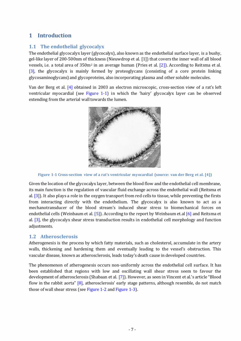
Van der Berg et al. [4] obtained in 2003 an electron microscopic, cross-section view of a rat’s left

ventricular myocardial (see Figure 1-1) in which the ‘hairy’ glycocalyx layer can be observed

extending from the arterial wall towards the lumen.

Figure 1-1 Cross-section view of a rat’s ventricular myocardial (source: van der Berg et al. [4])

Given the location of the glycocalyx layer, between the blood flow and the endothelial cell membrane,

its main function is the regulation of vascular fluid exchange across the endothelial wall (Reitsma et

al. [3]). It also plays a role in the oxygen transport from red cells to tissue, while preventing the firsts

from interacting directly with the endothelium. The glycocalyx is also known to act as a

mechanotransducer of the blood stream’s induced shear stress to biomechanical forces on

endothelial cells (Weinbaum et al. [5]). According to the report by Weinbaum et.al [6] and Reitsma et

al. [3], the glycocalyx shear stress transduction results in endothelial cell morphology and function

adjustments.

1.2 Atherosclerosis Atherogenesis is the process by which fatty materials, such as cholesterol, accumulate in the artery

walls, thickening and hardening them and eventually leading to the vessel’s obstruction. This

vascular disease, known as atherosclerosis, leads today’s death cause in developed countries.

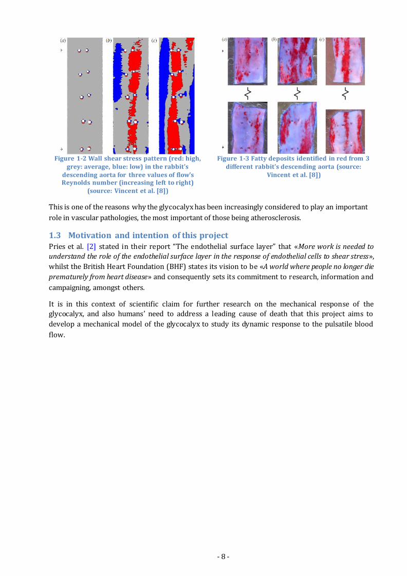
The phenomenon of atherogenesis occurs non-uniformly across the endothelial cell surface. It has

been established that regions with low and oscillating wall shear stress seem to favour the

development of atherosclerosis (Shabaan et al. [7]). However, as seen in Vincent et al.’s article “Blood

flow in the rabbit aorta” [8], atherosclerosis’ early stage patterns, although resemble, do not match

those of wall shear stress (see Figure 1-2 and Figure 1-3).

- 8 -

Figure 1-2 Wall shear stress pattern (red: high,

grey: average, blue: low) in the rabbit’s descending aorta for three values of flow’s Reynolds number (increasing left to right)

(source: Vincent et al. [8])

Figure 1-3 Fatty deposits identified in red from 3 different rabbit’s descending aorta (source:

Vincent et al. [8])

This is one of the reasons why the glycocalyx has been increasingly considered to play an important

role in vascular pathologies, the most important of those being atherosclerosis.

1.3 Motivation and intention of this project Pries et al. [2] stated in their report “The endothelial surface layer” that «More work is needed to

understand the role of the endothelial surface layer in the response of endothelial cells to shear stress»,

whilst the British Heart Foundation (BHF) states its vision to be «A world where people no longer die

prematurely from heart disease» and consequently sets its commitment to research, information and

campaigning, amongst others.

It is in this context of scientific claim for further research on the mechanical response of the

glycocalyx, and also humans’ need to address a leading cause of death that this project aims to

develop a mechanical model of the glycocalyx to study its dynamic response to the pulsatile blood

flow.

- 9 -

2 The one dimensional model In this chapter, the first approach to model mechanically the glycocalyx is discussed and

mathematically expressed. Furthermore, the solving process and final metric calculation are also

discussed.

To start with, a simplistic one dimensional (1D) model was developed in order to assess the

importance of the shear stress being pulsatile to the glycocalyx’ induced dynamics.

2.1 Model discussion For the reasons mentioned in 1 Introduction, the properties of the glycocalyx have been extensively

researched over the past decade. Yet, there is still some uncertainty on how its structure actually is

(Reitsma et al. [3]) and, specifically, how it behaves mechanically when exposed to the pulsatile

blood flow. That is why a very simplistic model was required: no unknown or uncertain properties

had to be implied by the developed mechanical model.

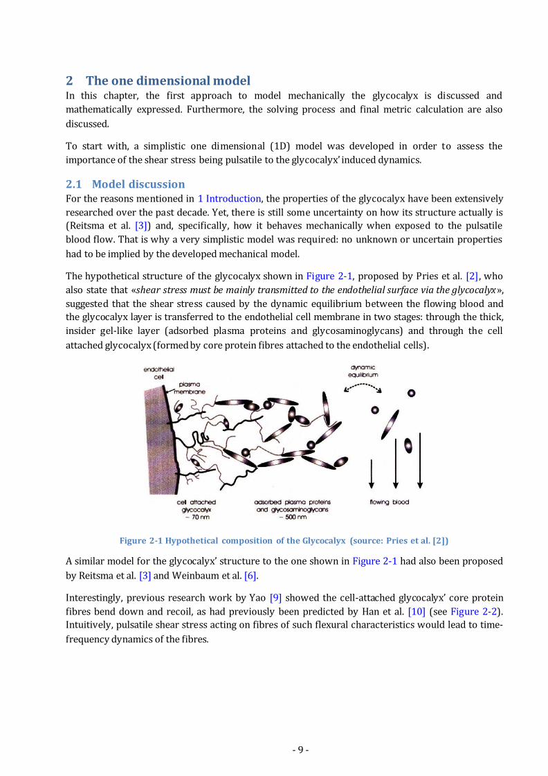
The hypothetical structure of the glycocalyx shown in Figure 2-1, proposed by Pries et al. [2], who

also state that «shear stress must be mainly transmitted to the endothelial surface via the glycocalyx»,

suggested that the shear stress caused by the dynamic equilibrium between the flowing blood and

the glycocalyx layer is transferred to the endothelial cell membrane in two stages: through the thick,

insider gel-like layer (adsorbed plasma proteins and glycosaminoglycans) and through the cell

attached glycocalyx (formed by core protein fibres attached to the endothelial cells).

Figure 2-1 Hypothetical composition of the Glycocalyx (source: Pries et al. [2])

A similar model for the glycocalyx’ structure to the one shown in Figure 2-1 had also been proposed

by Reitsma et al. [3] and Weinbaum et al. [6].

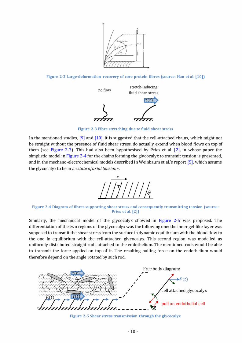
Interestingly, previous research work by Yao [9] showed the cell-attached glycocalyx’ core protein

fibres bend down and recoil, as had previously been predicted by Han et al. [10] (see Figure 2-2).

Intuitively, pulsatile shear stress acting on fibres of such flexural characteristics would lead to time-

frequency dynamics of the fibres.

- 10 -

Figure 2-2 Large-deformation recovery of core protein fibres (source: Han et al. [10])

Figure 2-3 Fibre stretching due to fluid shear stress

In the mentioned studies, [9] and [10], it is suggested that the cell-attached chains, which might not

be straight without the presence of fluid shear stress, do actually extend when blood flows on top of

them (see Figure 2-3). This had also been hypothesised by Pries et al. [2], in whose paper the

simplistic model in Figure 2-4 for the chains forming the glycocalyx to transmit tension is presented,

and in the mechano-electrochemical models described in Weinbaum et al.’s report [5], which assume

the glycocalyx to be in a «state of axial tension».

Figure 2-4 Diagram of fibres supporting shear stress and consequently transmitting tension (source: Pries et al. [2])

Similarly, the mechanical model of the glycocalyx showed in Figure 2-5 was proposed. The

differentiation of the two regions of the glycocalyx was the following one: the inner gel-like layer was

supposed to transmit the shear stress from the surface in dynamic equilibrium with the blood flow to

the one in equilibrium with the cell-attached glycocalyx. This second region was modelled as

uniformly distributed straight rods attached to the endothelium. The mentioned rods would be able

to transmit the force applied on top of it. The resulting pulling force on the endothelium would

therefore depend on the angle rotated by such rod.

𝜏(𝑡)

no flow stretch-inducing

fluid shear stress

Free body diagram: 𝜏(𝑡)

𝜏(𝑡) 𝐹(𝑡)

pull on endothelial cell

cell attached glycocalyx

𝐹(𝑡)

Figure 2-5 Shear stress transmission through the glycocalyx

- 11 -

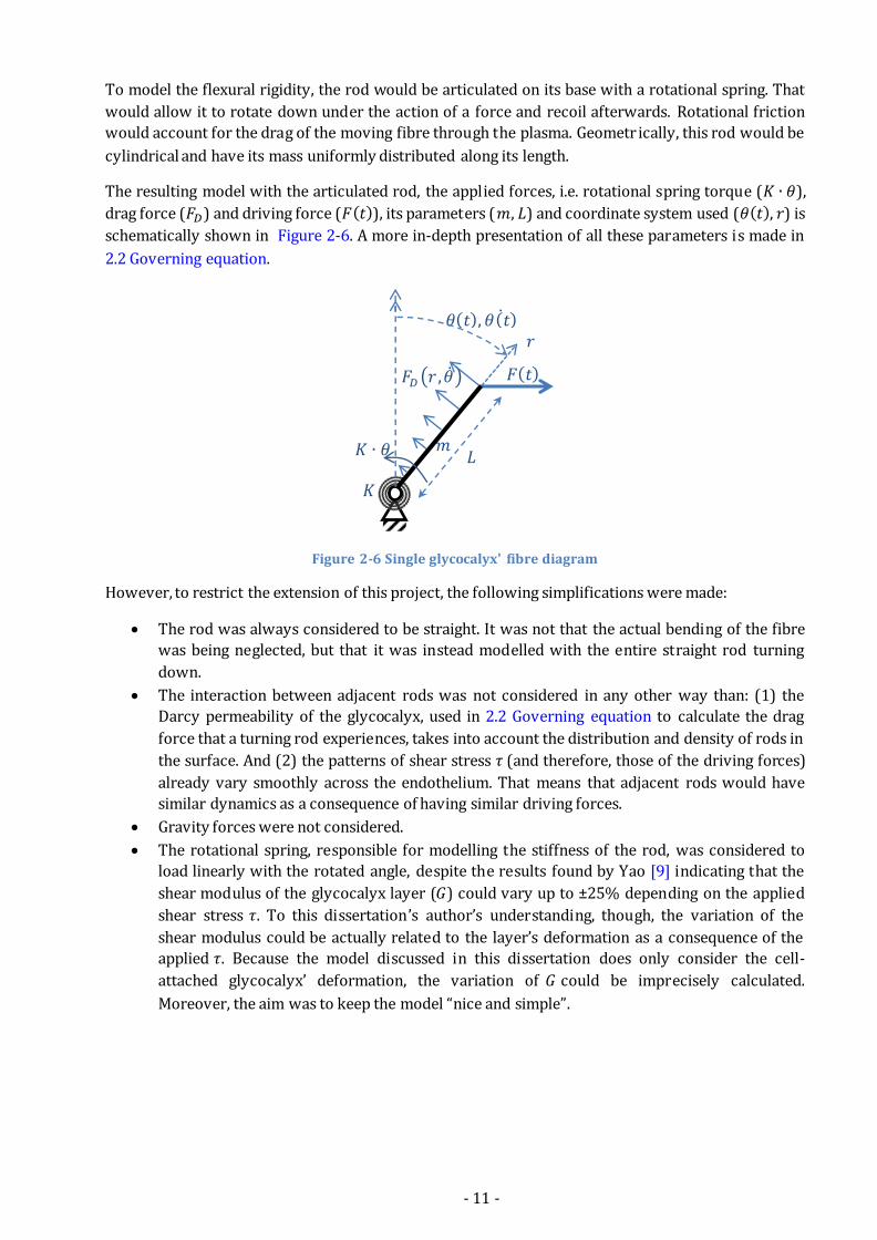
To model the flexural rigidity, the rod would be articulated on its base with a rotational spring. That

would allow it to rotate down under the action of a force and recoil afterwards. Rotational friction

would account for the drag of the moving fibre through the plasma. Geometr ically, this rod would be

cylindrical and have its mass uniformly distributed along its length.

The resulting model with the articulated rod, the applied forces, i.e. rotational spring torque ( ),

drag force ( ) and driving force ( ( )), its parameters ( , ) and coordinate system used ( ( ), ) is

schematically shown in Figure 2-6. A more in-depth presentation of all these parameters is made in

2.2 Governing equation.

Figure 2-6 Single glycocalyx' fibre diagram

However, to restrict the extension of this project, the following simplifications were made:

The rod was always considered to be straight. It was not that the actual bending of the fibre

was being neglected, but that it was instead modelled with the entire straight rod turning

down.

The interaction between adjacent rods was not considered in any other way than: (1) the

Darcy permeability of the glycocalyx, used in 2.2 Governing equation to calculate the drag

force that a turning rod experiences, takes into account the distribution and density of rods in

the surface. And (2) the patterns of shear stress (and therefore, those of the driving forces)

already vary smoothly across the endothelium. That means that adjacent rods would have

similar dynamics as a consequence of having similar driving forces.

Gravity forces were not considered.

The rotational spring, responsible for modelling the stiffness of the rod, was considered to

load linearly with the rotated angle, despite the results found by Yao [9] indicating that the

shear modulus of the glycocalyx layer ( ) could vary up to ±25% depending on the applied

shear stress . To this dissertation’s author’s understanding, though, the variation of the

shear modulus could be actually related to the layer’s deformation as a consequence of the

applied . Because the model discussed in this dissertation does only consider the cell-

attached glycocalyx’ deformation, the variation of could be imprecisely calculated.

Moreover, the aim was to keep the model “nice and simple”.

𝐹𝐷 𝑟 ,𝜃

𝑟

𝑚

𝐹(𝑡)

𝜃(𝑡), 𝜃(𝑡)

𝐿

𝐾

𝐾 𝜃

- 12 -

2.2 Governing equation The differential equation governing the aforementioned model is the following one:

( ) ( ) ( ) ( ) ( ) (Eq 2-1)

Where:

( ) is the angle rotated by the rod [ ].

is the inertia of the rod [ ], which depends on its mass ( [ ]) and length ( [ ]). The

corresponding cylinder inertia is:

(Eq 2-2)

is the coefficient of rotational friction [

], modelling the drag force experienced by the

turning rod in the plasma-like media. According to Weinbaum et al. [5], such drag force [ ]

can be calculated as follows:

,

(Eq 2-3)

Here is the plasma viscosity [ ], is the fibre radius [ ], is the fibre volume fraction

[ ], is the Darcy permeability of the glycocalyx [ ] and is the fibre gap [ ].

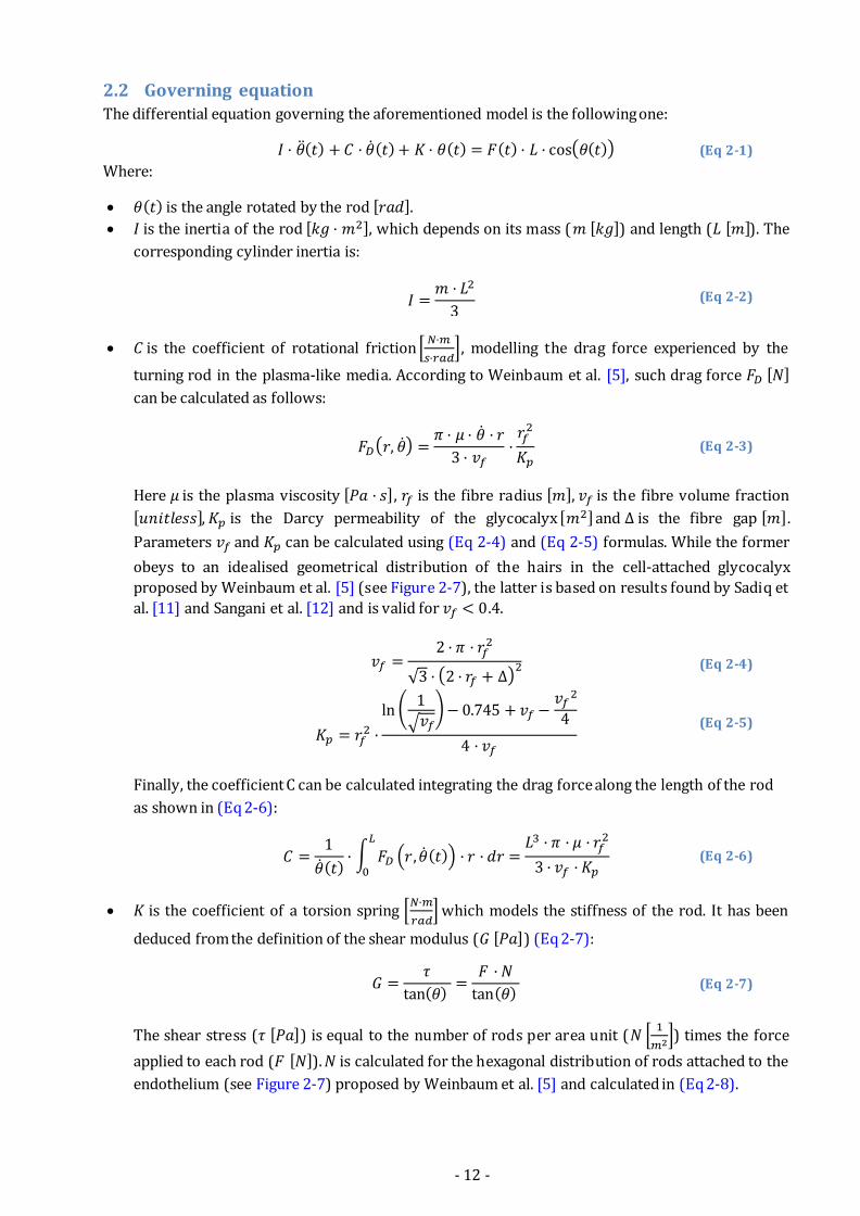
Parameters and can be calculated using (Eq 2-4) and (Eq 2-5) formulas. While the former

obeys to an idealised geometrical distribution of the hairs in the cell-attached glycocalyx

proposed by Weinbaum et al. [5] (see Figure 2-7), the latter is based on results found by Sadiq et

al. [11] and Sangani et al. [12] and is valid for .

√ (Eq 2-4)

(

√ )

(Eq 2-5)

Finally, the coefficient C can be calculated integrating the drag force along the length of the rod

as shown in (Eq 2-6):

( ) ∫ ( , ( ))

(Eq 2-6)

is the coefficient of a torsion spring [

] which models the stiffness of the rod. It has been

deduced from the definition of the shear modulus ( [ ]) (Eq 2-7):

( )

( ) (Eq 2-7)

The shear stress ( [ ]) is equal to the number of rods per area unit ( [

]) times the force

applied to each rod ( [ ]). is calculated for the hexagonal distribution of rods attached to the

endothelium (see Figure 2-7) proposed by Weinbaum et al. [5] and calculated in (Eq 2-8).

- 13 -

Figure 2-7 Idealised geometrical distribution of rods on the endothelium

√ (Eq 2-8)

Linearizing (Eq 2-7) for with: ( )

, the formula in (Eq 2-9) for the coefficient

K is obtained:

(Eq 2-9)

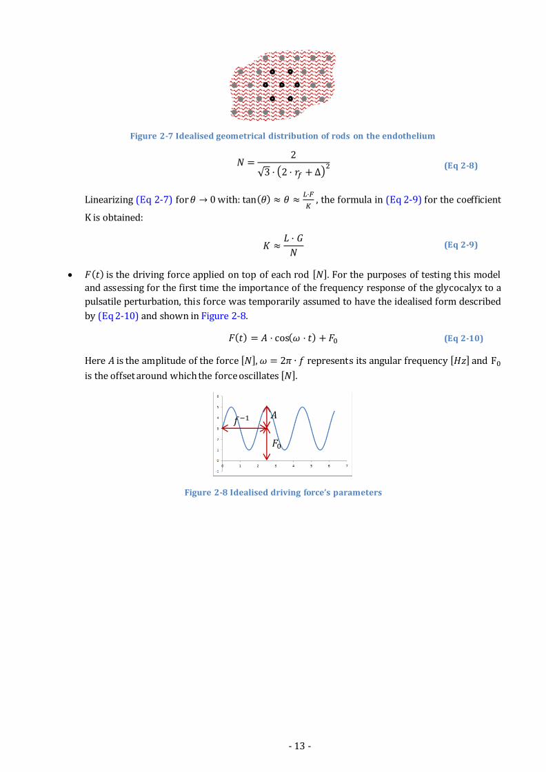
( ) is the driving force applied on top of each rod [ ]. For the purposes of testing this model

and assessing for the first time the importance of the frequency response of the glycocalyx to a

pulsatile perturbation, this force was temporarily assumed to have the idealised form described

by (Eq 2-10) and shown in Figure 2-8.

( ) ( ) (Eq 2-10)

Here is the amplitude of the force [ ], represents its angular frequency [ ] and

is the offset around which the force oscillates [ ].

Figure 2-8 Idealised driving force’s parameters

𝑓− 𝐴

𝐹

- 14 -

2.3 Model parameter values The parameters that appear in the governing equation depend on the characteristics of the

glycocalyx. Table 2-1 shows these characterising parameters and the references that were used to

determine them.

Description Parameter value Comments Rod’s mass − According to Reitsma et al. [3], high-weight

glycosaminoglycan chains present in the glycocalyx have a mass of up to 104 kDa.

Rod’s length − Pries et al. [2] stated the thickness of the glycocalyx to be comprised between 70nm and 400nm, being the lowest value the one associated with the cell-attached glycocalyx.

Plasma viscosity − Value of the blood plasma viscosity measured by Haidekker et al. [13] using fluorescent molecular rotors.

Fibre gap − From the structural model of the glycocalyx presented in Weinbaum et al. [5], consistent with results from Curry et al. [14] (center-to-center spacing around 20 nm)

Fibre radius −

Shear modulus Yao [9], calculated it using an imaging technique tracing the motion of quantum dots attached to the glycocalyx and stated that .

Table 2-1 Defining parameters: glycocalyx characteristics

As a result, dependant parameters shown in Table 2-2, and particularly , and (highlighted in

blue) which appear in the governing equation, could be calculated:

Description Parameter value Comments Rod’s inertia − Fibre volume fraction

Validates the equation (Eq 2-5) for the Darcy permeability of the glycocalyx ( ).

Darcy permeability of the glycocalyx

− In some references, and particularly in the article by Sadiq et al. [11], it is also expressed as the non-dimensional parameter

− [ ].

Rotational friction coefficient

−

Number of rods per area unit

Rotational spring coefficient

−

Table 2-2 Calculated parameters, including I, C and K

2.4 Simplification of the governing equation

From the results in Table 2-2 it turned out that: − , − . Therefore, the governing

equation could be simplified by omitting to the first-order, nonlinear differential equation shown in

(Eq 2-11):

( ) ( ) ( ) ( ) (Eq 2-11)

- 15 -

2.5 Non-dimensionalisation Given the high dependence of the governing equation’s parameters on the characteristics of the

glycocalyx, it was a good practice to non-dimensionalise it in a convenient manner. Using (Eq 2-10) in

(Eq 2-11) and dividing the resulting equation by one obtains (Eq 2-12):

( ) ( )

( ( ) ) ( ) (Eq 2-12)

The new non-dimensional parameters were defined in (Eq 2-13) to (Eq 2-15):

,

[ ] (Eq 2-13)

[ ] (Eq 2-14)

,

[ ] (Eq 2-15)

Consequently, the governing equation could be expressed in terms of these new parameters and

variable as follows:

( ) ( ) ( ) ( ) (Eq 2-16)

A solution of this equation would therefore be valid for the chosen values of , and , which can

correspond to different combinations of the actual characteristics of the glycocalyx (length, spacing,

stiffness…). Hence, the convenience of this non-dimensionalisation.

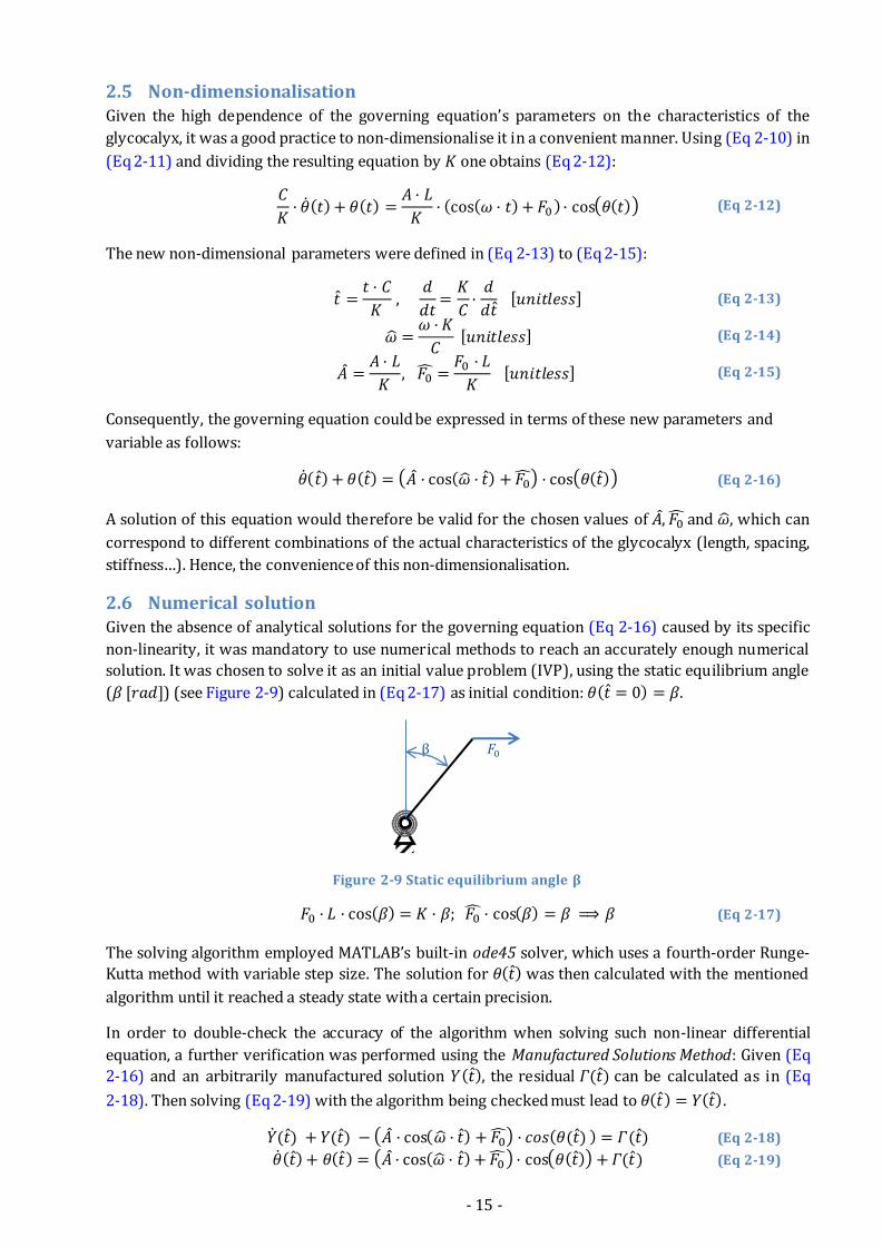
2.6 Numerical solution Given the absence of analytical solutions for the governing equation (Eq 2-16) caused by its specific

non-linearity, it was mandatory to use numerical methods to reach an accurately enough numerical

solution. It was chosen to solve it as an initial value problem (IVP), using the static equilibrium angle

( [ ]) (see Figure 2-9) calculated in (Eq 2-17) as initial condition: ( ) .

Figure 2-9 Static equilibrium angle β

( ) ( ) ⇒ (Eq 2-17)

The solving algorithm employed MATLAB’s built-in ode45 solver, which uses a fourth-order Runge-

Kutta method with variable step size. The solution for ( ) was then calculated with the mentioned

algorithm until it reached a steady state with a certain precision.

In order to double-check the accuracy of the algorithm when solving such non-linear differential

equation, a further verification was performed using the Manufactured Solutions Method: Given (Eq

2-16) and an arbitrarily manufactured solution ( ), the residual ( ) can be calculated as in (Eq

2-18). Then solving (Eq 2-19) with the algorithm being checked must lead to ( ) ( ).

( ) ( ) ( ) ( ( ) ) ( ) (Eq 2-18)

( ) ( ) ( ) ( ) ( ) (Eq 2-19)

𝐹 β

- 16 -

In regards to the values of the non-dimensional parameters appearing in the equation to be solved,

(Eq 2-16), a range of them was chosen for each parameter in order to generate a map of solutions

(see 3 1D model results). Table 2-3 specifies these parameters’ ranges:

Parameters’ values Comments

It corresponds approximately to , which according to [15] is a sensible range.

Corresponding to , the range of shear stress values found in simulations by [16].

Table 2-3 Ranges for the non-dimensional parameters

2.7 Post-processing Once each solution of ( ) for a certain combination of values of the non-dimensional parameters

had been found, a further calculation was performed in order to determine the actual pull being

transferred to the endothelial cell membrane. This calculation consisted in taking the driving force in

the direction of the rod ( ) (Eq 2-20) and integrating it through all the intervals within one period

of the steady state for which the rod was under traction (Eq 2-21).

( ) ( ) ( ) ( ) ( ) (Eq 2-20)

∑∫ ( ) { , }

(Eq 2-21)

In (Eq 2-21), is an ascending integer number (0, 1, 2…), is the value of for which

( ) , is an arbitrary value of for which ( ) has reached the steady state,

is the

non-dimensional oscillation period of both the driving force and the rod’s turned angle, and

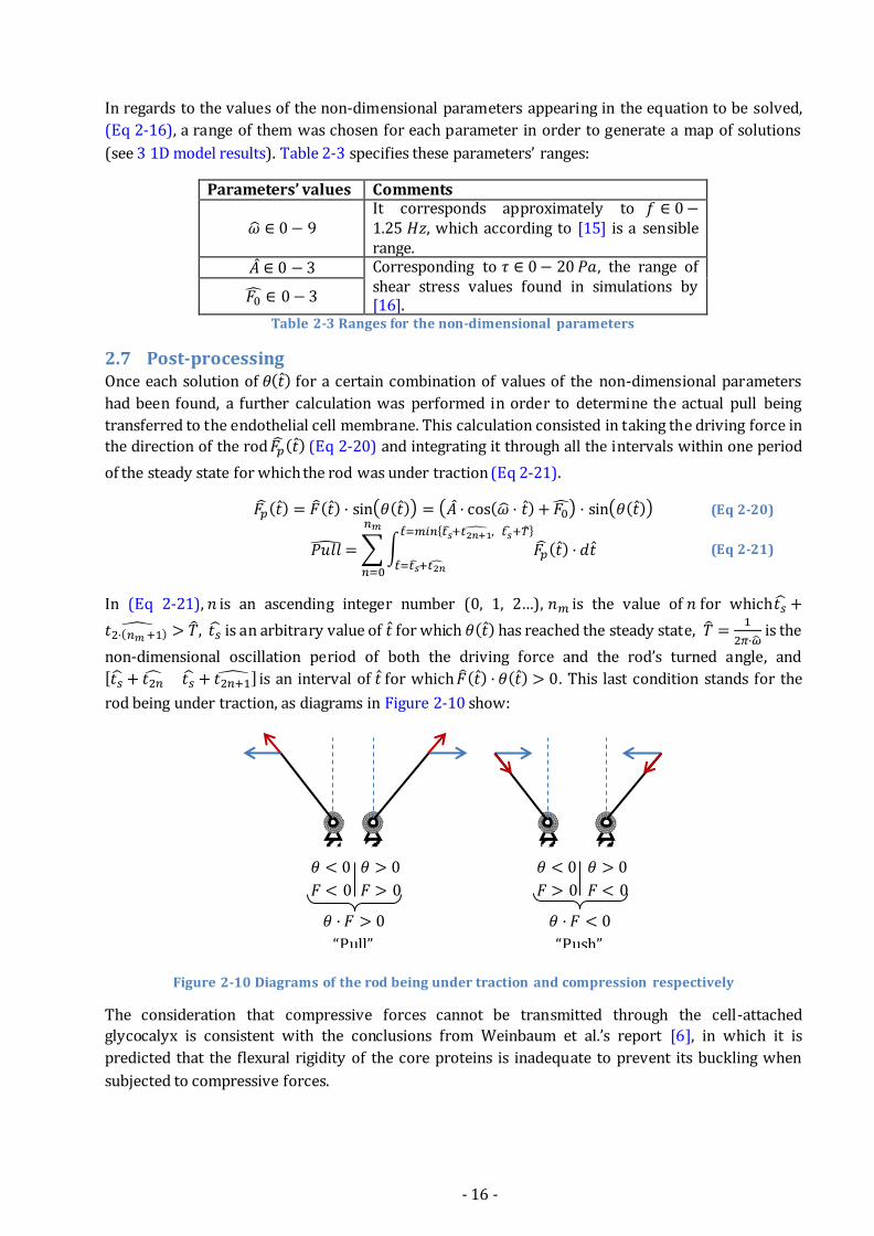
[ ] is an interval of for which ( ) ( ) . This last condition stands for the

rod being under traction, as diagrams in Figure 2-10 show:

Figure 2-10 Diagrams of the rod being under traction and compression respectively

The consideration that compressive forces cannot be transmitted through the cell-attached

glycocalyx is consistent with the conclusions from Weinbaum et al.’s report [6], in which it is

predicted that the flexural rigidity of the core proteins is inadequate to prevent its buckling when

subjected to compressive forces.

𝜃

𝐹

𝜃

𝐹

𝜃 𝐹

“Push”

𝜃

𝐹

𝜃

𝐹

𝜃 𝐹

“Pull”

- 17 -

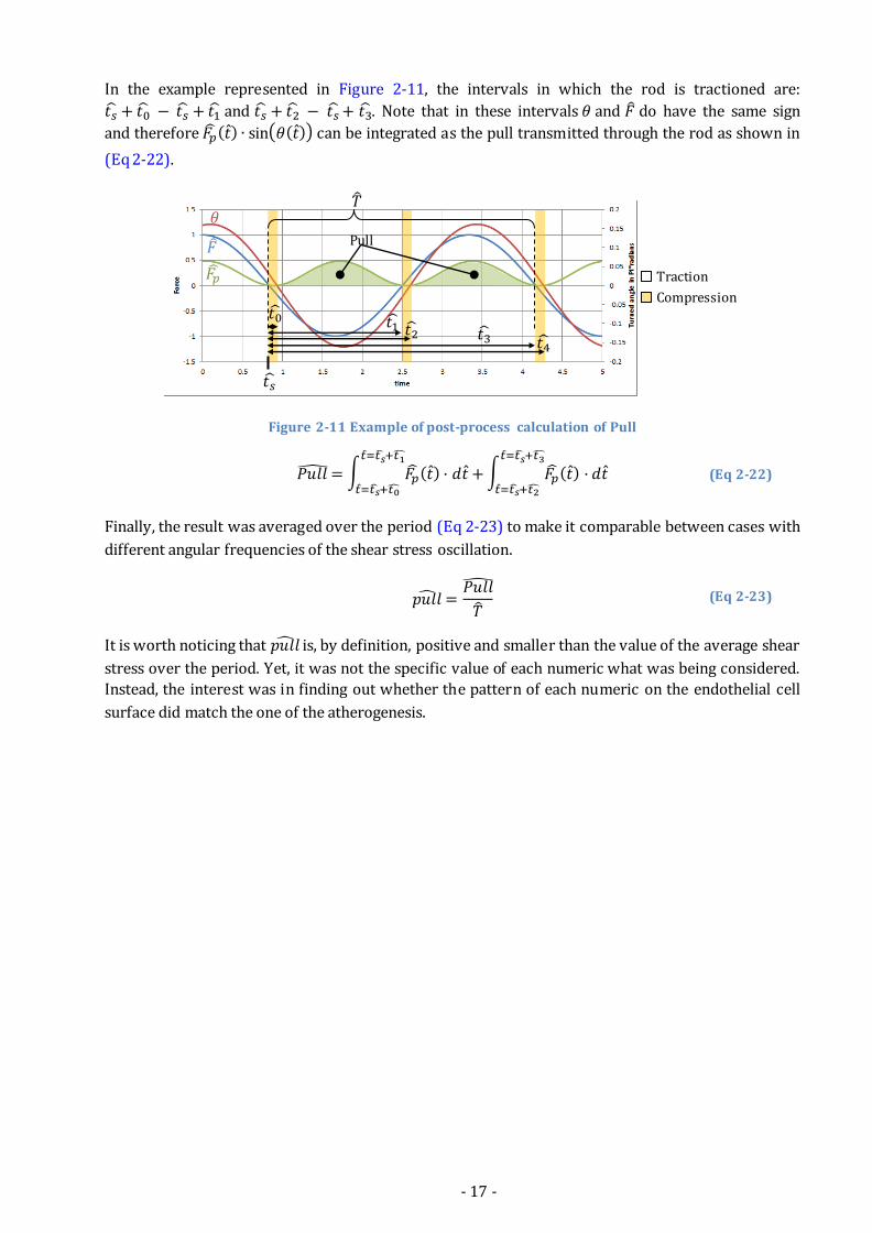
In the example represented in Figure 2-11, the intervals in which the rod is tractioned are:

and . Note that in these intervals and do have the same sign

and therefore ( ) ( ) can be integrated as the pull transmitted through the rod as shown in

(Eq 2-22).

Figure 2-11 Example of post-process calculation of Pull

∫ ( )

∫ ( )

(Eq 2-22)

Finally, the result was averaged over the period (Eq 2-23) to make it comparable between cases with

different angular frequencies of the shear stress oscillation.

(Eq 2-23)

It is worth noticing that is, by definition, positive and smaller than the value of the average shear

stress over the period. Yet, it was not the specific value of each numeric what was being considered.

Instead, the interest was in finding out whether the pattern of each numeric on the endothelial cell

surface did match the one of the atherogenesis.

𝐹��

��

𝜃 ��

Traction

Compression

Pull

𝑡��

𝑡 𝑡 𝑡 𝑡

𝑡4

- 19 -

3 1D model results Results obtained from solving the rod’s steady state dynamic response to different pulsatile driving

forces (for different values of , and ) were used to calculate the transferred force ( ) in each

case. Such results were vast and thus, laborious to analyse at a first glance. In this chapter, they are

presented and analysed in different “slices”. All 1D results were calculated using the non-

dimensionalising parameter values from 2.3 Model parameter values.

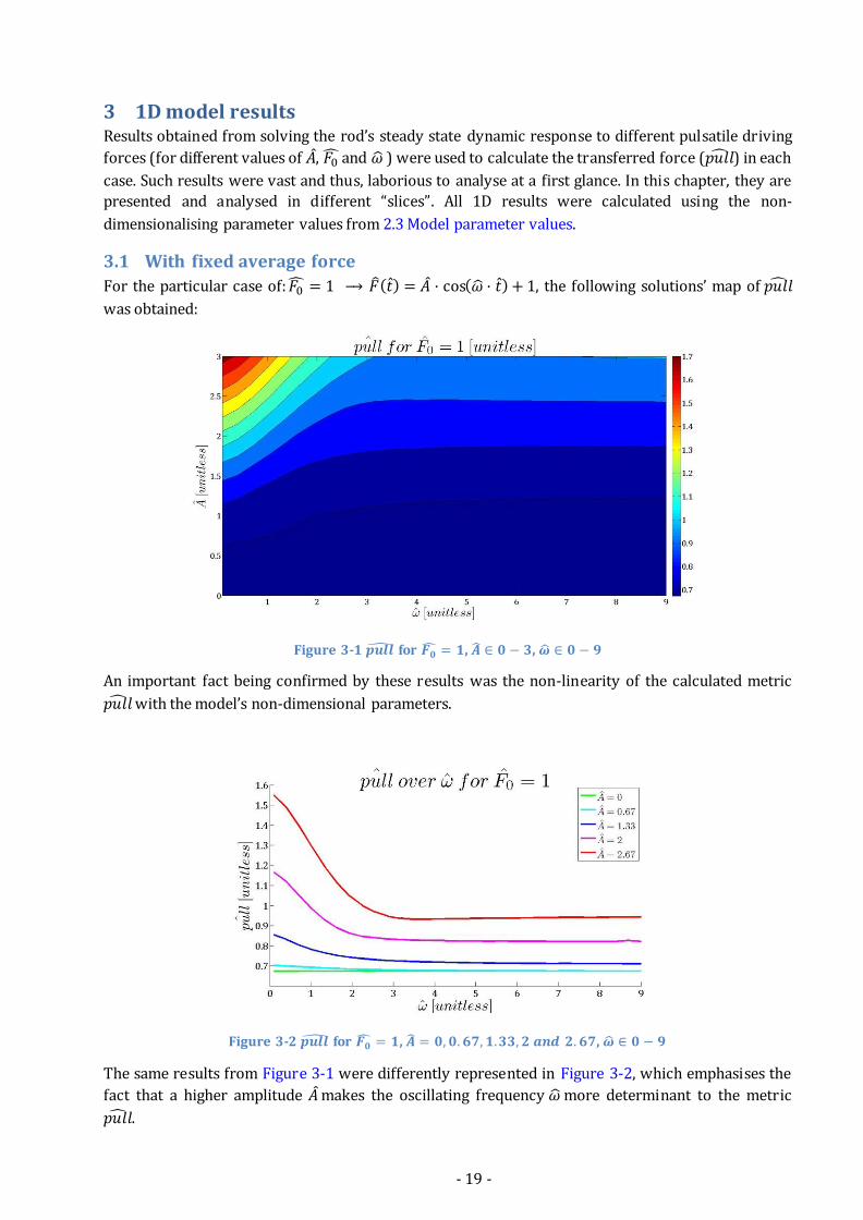
3.1 With fixed average force

For the particular case of: → ( ) ( ) , the following solutions’ map of

was obtained:

Figure 3-1 for , ,

An important fact being confirmed by these results was the non-linearity of the calculated metric

with the model’s non-dimensional parameters.

Figure 3-2 for , , , , ,

The same results from Figure 3-1 were differently represented in Figure 3-2, which emphasises the

fact that a higher amplitude makes the oscillating frequency more determinant to the metric

.

- 20 -

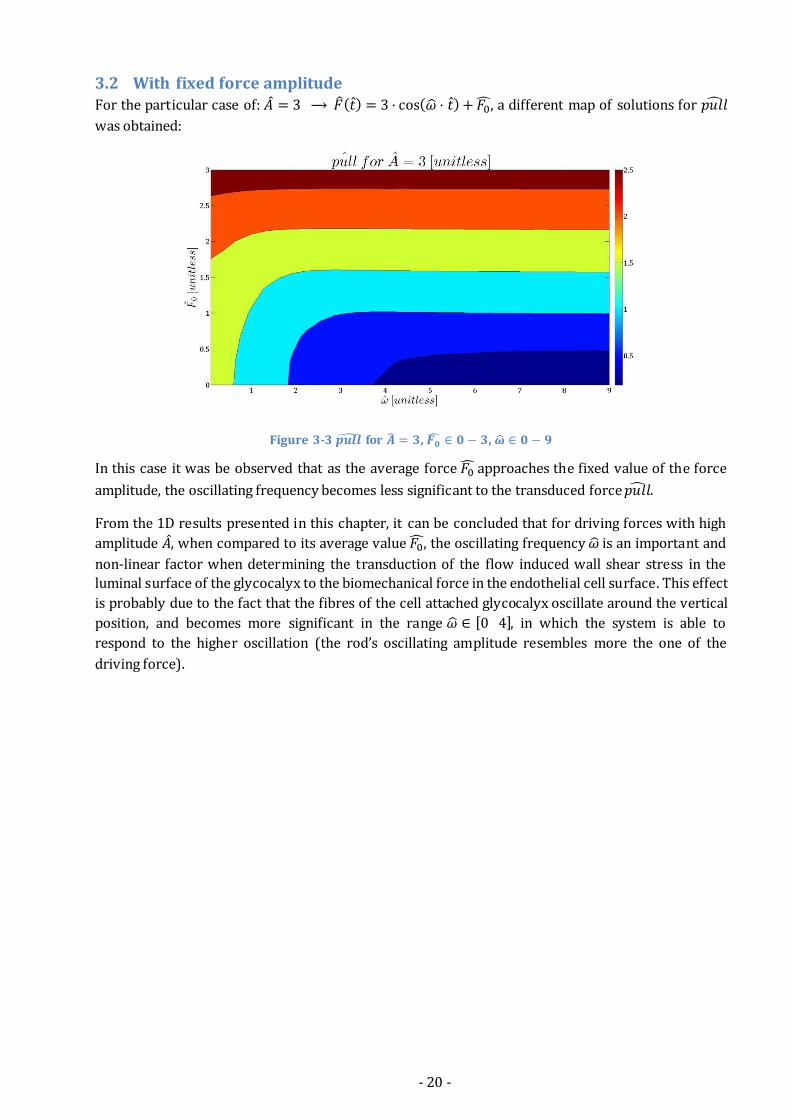
3.2 With fixed force amplitude For the particular case of:

→ ( ) ( ) , a different map of solutions for

was obtained:

Figure 3-3 for , ,

In this case it was be observed that as the average force approaches the fixed value of the force

amplitude, the oscillating frequency becomes less significant to the transduced force .

From the 1D results presented in this chapter, it can be concluded that for driving forces with high

amplitude , when compared to its average value , the oscillating frequency is an important and

non-linear factor when determining the transduction of the flow induced wall shear stress in the

luminal surface of the glycocalyx to the biomechanical force in the endothelial cell surface. This effect

is probably due to the fact that the fibres of the cell attached glycocalyx oscillate around the vertical

position, and becomes more significant in the range [ ], in which the system is able to

respond to the higher oscillation (the rod’s oscillating amplitude resembles more the one of the

driving force).

- 21 -

4 The two dimensional model Having explored the importance of the frequency response of the 1D model of the glycocalyx, the

next step was to post-process a larger, more realistic set of shear stress data. Although this larger set

of data was three dimensional, simplifications described in 2.1 Model discussion allowed to post-

process it using a two dimensional (2D) model. In other words, since interactions between adjacent

rods were not considered, each one could be processed regardless of its position and orientation.

Hence, an extension of the previous model to 2D was discussed and mathematically defined.

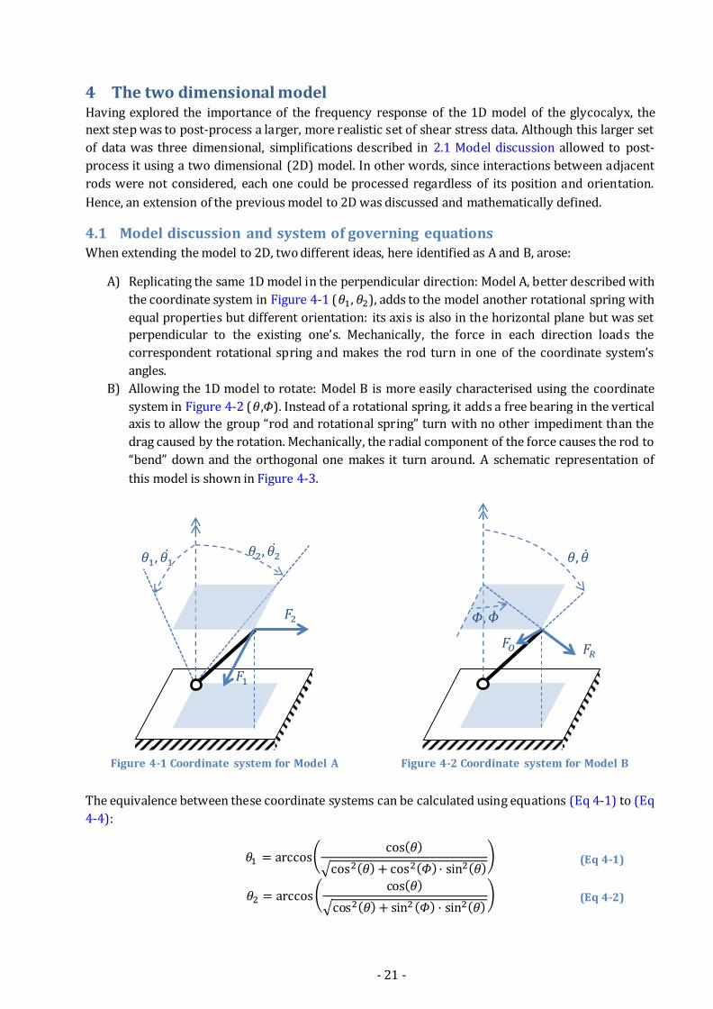
4.1 Model discussion and system of governing equations When extending the model to 2D, two different ideas, here identified as A and B, arose:

A) Replicating the same 1D model in the perpendicular direction: Model A, better described with

the coordinate system in Figure 4-1 ( , ), adds to the model another rotational spring with

equal properties but different orientation: its axis is also in the horizontal plane but was set

perpendicular to the existing one’s. Mechanically, the force in each direction loads the

correspondent rotational spring and makes the rod turn in one of the coordinate system’s

angles.

B) Allowing the 1D model to rotate: Model B is more easily characterised using the coordinate

system in Figure 4-2 ( , ). Instead of a rotational spring, it adds a free bearing in the vertical

axis to allow the group “rod and rotational spring” turn with no other impediment than the

drag caused by the rotation. Mechanically, the radial component of the force causes the rod to

“bend” down and the orthogonal one makes it turn around. A schematic representation of

this model is shown in Figure 4-3.

Figure 4-1 Coordinate system for Model A Figure 4-2 Coordinate system for Model B

The equivalence between these coordinate systems can be calculated using equations (Eq 4-1) to (Eq

4-4):

( ( )

√ ( ) ( ) ( )) (Eq 4-1)

( ( )

√ ( ) ( ) ( )) (Eq 4-2)

𝐹

𝜃 , 𝜃 𝜃 , 𝜃

𝐹

𝜃, 𝜃

𝛷,𝛷

𝐹𝑅 𝐹𝑂

- 22 -

( ( ) ( )

√ ( ) ( ) ( )

) (Eq 4-3)

( ( ) ( )

√ ( ) ( ) ( )

( )) (Eq 4-4)

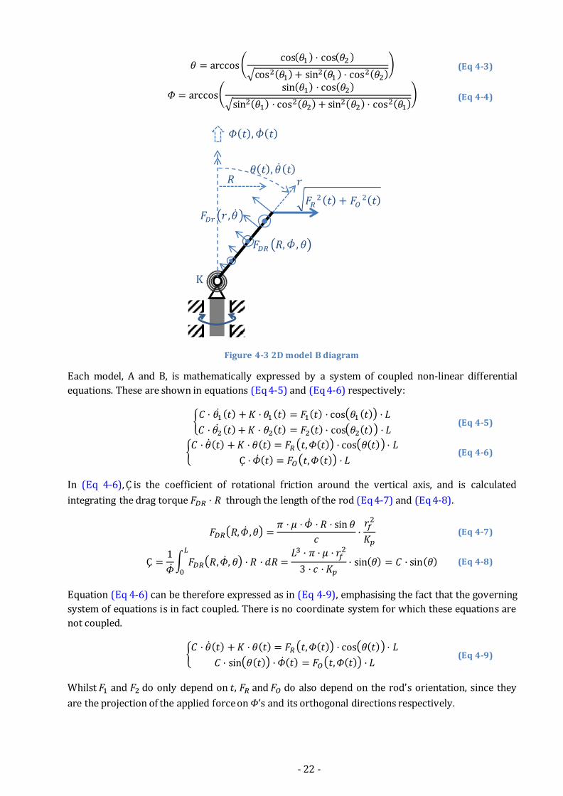
Figure 4-3 2D model B diagram

Each model, A and B, is mathematically expressed by a system of coupled non-linear differential

equations. These are shown in equations (Eq 4-5) and (Eq 4-6) respectively:

{ ( ) ( ) ( ) ( )

( ) ( ) ( ) ( ) (Eq 4-5)

{ ( ) ( ) , ( ) ( )

( ) , ( ) (Eq 4-6)

In (Eq 4-6), is the coefficient of rotational friction around the vertical axis, and is calculated

integrating the drag torque through the length of the rod (Eq 4-7) and (Eq 4-8).

, ,

(Eq 4-7)

∫ , ,

( ) ( ) (Eq 4-8)

Equation (Eq 4-6) can be therefore expressed as in (Eq 4-9), emphasising the fact that the governing

system of equations is in fact coupled. There is no coordinate system for which these equations are

not coupled.

{ ( ) ( ) , ( ) ( )

( ) ( ) , ( ) (Eq 4-9)

Whilst and do only depend on , and do also depend on the rod’s orientation, since they

are the projection of the applied force on ’s and its orthogonal directions respectively.

𝑅

𝛷(𝑡),𝛷 (𝑡)

𝐹𝐷𝑟 𝑟 ,𝜃

𝑟

𝐹𝑅 (𝑡) 𝐹𝑂

(𝑡)

𝜃(𝑡), 𝜃 (𝑡)

K

𝐹𝐷𝑅 𝑅,𝛷 , 𝜃

- 23 -

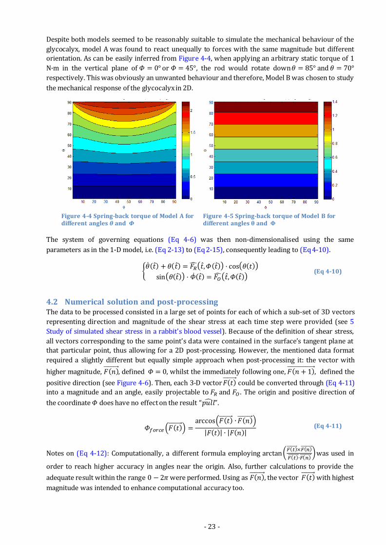
Despite both models seemed to be reasonably suitable to simulate the mechanical behaviour of the

glycocalyx, model A was found to react unequally to forces with the same magnitude but different

orientation. As can be easily inferred from Figure 4-4, when applying an arbitrary static torque of 1

N·m in the vertical plane of or , the rod would rotate down and

respectively. This was obviously an unwanted behaviour and therefore, Model B was chosen to study

the mechanical response of the glycocalyx in 2D.

Figure 4-4 Spring-back torque of Model A for different angles and

Figure 4-5 Spring-back torque of Model B for different angles θ and Φ

The system of governing equations (Eq 4-6) was then non-dimensionalised using the same

parameters as in the 1-D model, i.e. (Eq 2-13) to (Eq 2-15), consequently leading to (Eq 4-10).

{ ( ) ( ) , ( ) ( )

( ) ( ) , ( ) (Eq 4-10)

4.2 Numerical solution and post-processing The data to be processed consisted in a large set of points for each of which a sub-set of 3D vectors

representing direction and magnitude of the shear stress at each time step were provided (see 5

Study of simulated shear stress in a rabbit’s blood vessel). Because of the definition of shear stress,

all vectors corresponding to the same point’s data were contained in the surface’s tangent plane at

that particular point, thus allowing for a 2D post-processing. However, the mentioned data format

required a slightly different but equally simple approach when post-processing it: the vector with

higher magnitude, ( ) , defined , whilst the immediately following one, ( ) , defined the

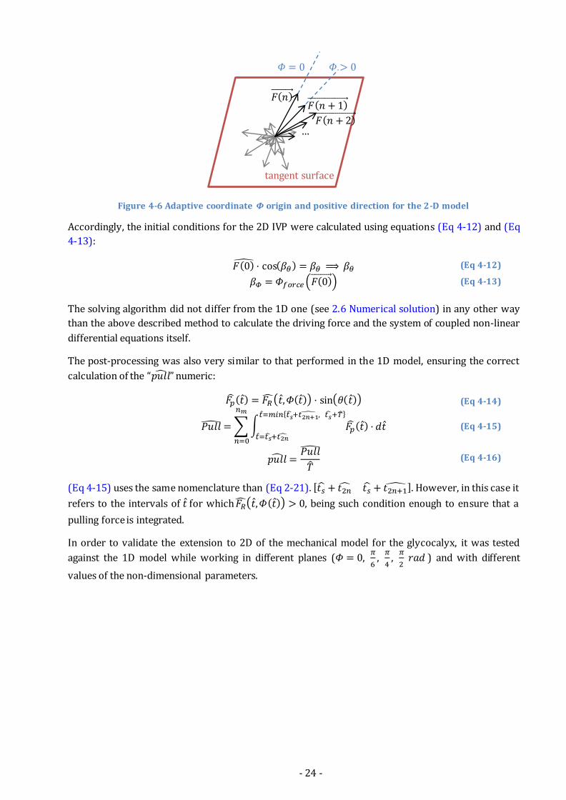
positive direction (see Figure 4-6). Then, each 3-D vector ( ) could be converted through (Eq 4-11)

into a magnitude and an angle, easily projectable to and . The origin and positive direction of

the coordinate does have no effect on the result “ ”.

( ( ) )

( ( ) ( ) )

| ( )| | ( )| (Eq 4-11)

Notes on (Eq 4-12): Computationally, a different formula employing ( ( ) ( )

( ) ( ) ) was used in

order to reach higher accuracy in angles near the origin. Also, further calculations to provide the

adequate result within the range were performed. Using as ( ) , the vector ( ) with highest

magnitude was intended to enhance computational accuracy too.

- 24 -

Figure 4-6 Adaptive coordinate origin and positive direction for the 2-D model

Accordingly, the initial conditions for the 2D IVP were calculated using equations (Eq 4-12) and (Eq

4-13):

( ) ( ) ⇒ (Eq 4-12)

( ( ) ) (Eq 4-13)

The solving algorithm did not differ from the 1D one (see 2.6 Numerical solution) in any other way

than the above described method to calculate the driving force and the system of coupled non-linear

differential equations itself.

The post-processing was also very similar to that performed in the 1D model, ensuring the correct

calculation of the “ ” numeric:

( ) , ( ) ( ) (Eq 4-14)

∑∫ ( ) { , }

(Eq 4-15)

(Eq 4-16)

(Eq 4-15) uses the same nomenclature than (Eq 2-21). [ ] However, in this case it

refers to the intervals of for which , ( ) , being such condition enough to ensure that a

pulling force is integrated.

In order to validate the extension to 2D of the mechanical model for the glycocalyx, it was tested

against the 1D model while working in different planes ( ,

,

4,

) and with different

values of the non-dimensional parameters.

tangent surface

𝐹(𝑛) 𝐹(𝑛 )

𝐹(𝑛 ) …

𝛷 𝛷

- 25 -

5 Study of simulated shear stress in a rabbit’s blood vessel The 2D model had been prepared to post-process simulated data from a 3D geometry, with which

more realistic results and conclusions could be obtained. Before presenting the results of such study,

though, considerations regarding the original data and the different cases considered are made in the

following section:

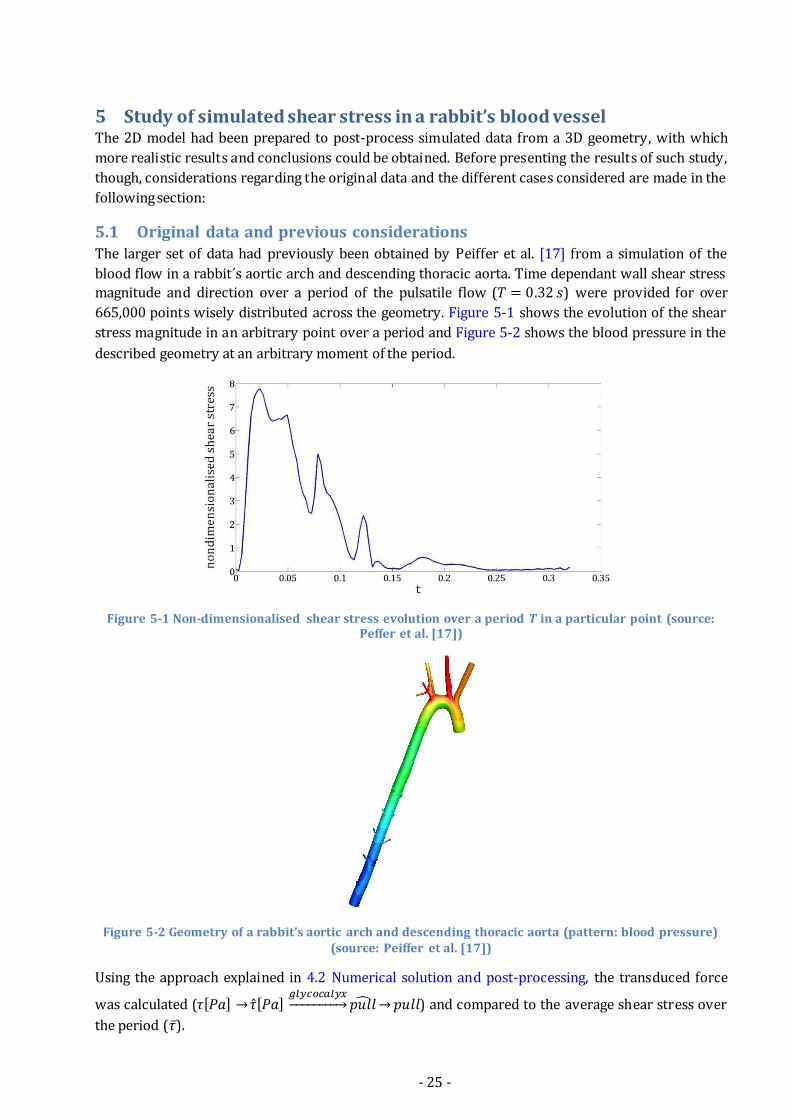
5.1 Original data and previous considerations The larger set of data had previously been obtained by Peiffer et al. [17] from a simulation of the

blood flow in a rabbit´s aortic arch and descending thoracic aorta. Time dependant wall shear stress

magnitude and direction over a period of the pulsatile flow ( ) were provided for over

665,000 points wisely distributed across the geometry. Figure 5-1 shows the evolution of the shear

stress magnitude in an arbitrary point over a period and Figure 5-2 shows the blood pressure in the

described geometry at an arbitrary moment of the period.

Figure 5-1 Non-dimensionalised shear stress evolution over a period in a particular point (source: Peffer et al. [17])

Figure 5-2 Geometry of a rabbit’s aortic arch and descending thoracic aorta (pattern: blood pressure) (source: Peiffer et al. [17])

Using the approach explained in 4.2 Numerical solution and post-processing, the transduced force

was calculated ( [ ] [ ] → ) and compared to the average shear stress over

the period ( ).

- 26 -

Firstly, a much reduced set of 11 points was chosen both to check the model and to extract the first

conclusions. Secondly, a larger set of -data corresponding to a cropped section of the geometry

(including over 70,700 points, that is 10% of the whole set) was also studied. This cropped geometry

corresponds to a region of the descending thoracic aorta including two intercostal branches. In both

studies, different combinations of the glycocalyx defining parameters (including the baseline case)

were considered.

In the non-dimensionalisation defined by (Eq 2-13) to (Eq 2-15), two dimensional reference

magnitudes had been used: the reference time ( [ ]) (Eq 5-1), and the reference force ( [ ]).

The latter is expressed in (Eq 5-2) as reference shear stress ( [ ]). These reference

magnitudes account for the glycocalyx properties in the non-dimensional model.

(Eq 5-1)

(Eq 5-2)

Note that, from (Eq 2-13), (Eq 2-15), (Eq 5-1) and (Eq 5-2)

and

. Therefore

⁄ ( )

. Equivalently, one can re-dimensionalise as follows: [ ] .

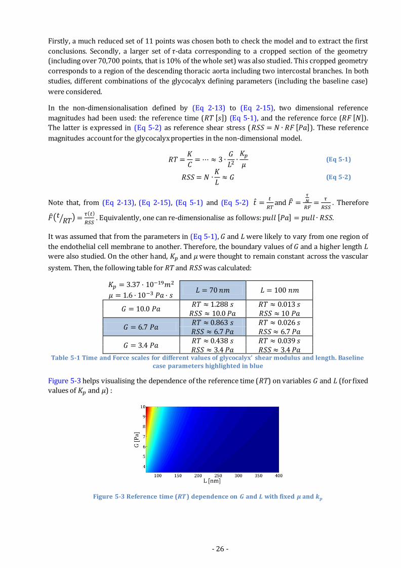
It was assumed that from the parameters in (Eq 5-1), and were likely to vary from one region of

the endothelial cell membrane to another. Therefore, the boundary values of and a higher length

were also studied. On the other hand, and were thought to remain constant across the vascular

system. Then, the following table for and was calculated:

−

−

Table 5-1 Time and Force scales for different values of glycocalyx’ shear modulus and length. Baseline case parameters highlighted in blue

Figure 5-3 helps visualising the dependence of the reference time ( ) on variables and (for fixed

values of and ) :

Figure 5-3 Reference time ( ) dependence on and with fixed and

- 27 -

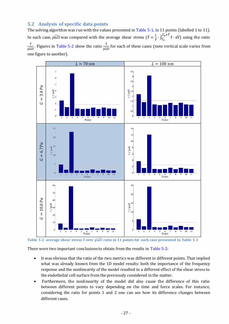
5.2 Analysis of specific data points The solving algorithm was run with the values presented in Table 5-1, in 11 points (labelled 1 to 11).

In each case, was compared with the average shear stress (

∫

) using the ratio

. Figures in Table 5-2 show the ratio

for each of these cases (note vertical scale varies from

one figure to another).

Table 5-2 average shear stress over ratio in 11 points for each case presented in Table 5-1

There were two important conclusions to obtain from the results in Table 5-2:

It was obvious that the ratio of the two metrics was different in different points. That implied

what was already known from the 1D model results: both the importance of the frequency

response and the nonlinearity of the model resulted in a different effect of the shear stress to

the endothelial cell surface from the previously considered in the matter.

Furthermore, the nonlinearity of the model did also cause the difference of this ratio

between different points to vary depending on the time and force scales. For instance,

considering the ratio for points 1 and 2 one can see how its difference changes between

different cases.

- 28 -

Although these conclusions could make one think that the two patterns of and would indeed

differ, it was important to realise that it could also be the case that smaller differences between both

patterns, such as sharpening or smoothening would be obtained.

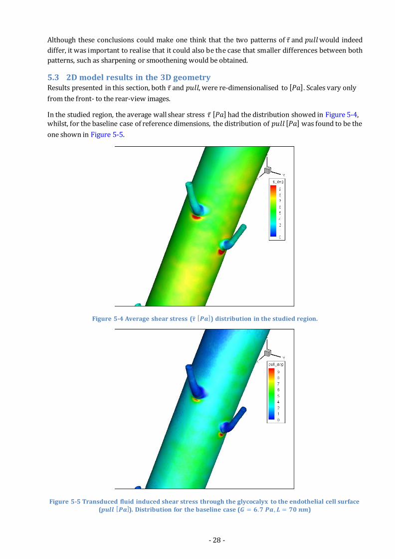
5.3 2D model results in the 3D geometry Results presented in this section, both and , were re-dimensionalised to [ ]. Scales vary only

from the front- to the rear-view images.

In the studied region, the average wall shear stress [ ] had the distribution showed in Figure 5-4, whilst, for the baseline case of reference dimensions, the distribution of [ ] was found to be the

one shown in Figure 5-5.

Figure 5-4 Average shear stress ( [ ]) distribution in the studied region.

Figure 5-5 Transduced fluid induced shear stress through the glycocalyx to the endothelial cell surface ( [ ]). Distribution for the baseline case ( , )

- 29 -

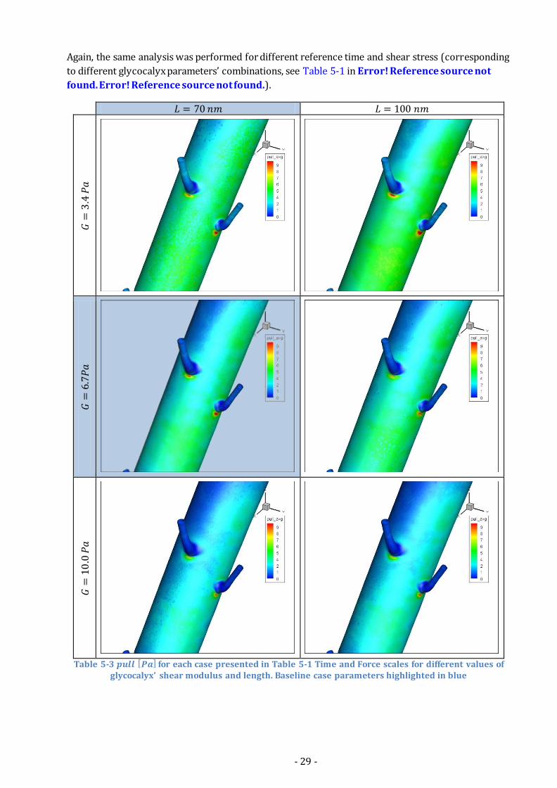
Again, the same analysis was performed for different reference time and shear stress (corresponding

to different glycocalyx parameters’ combinations, see Table 5-1 in Error! Reference source not

found. Error! Reference source not found.).

Table 5-3 [ ] for each case presented in Table 5-1 Time and Force scales for different values of

glycocalyx’ shear modulus and length. Baseline case parameters highlighted in blue

- 30 -

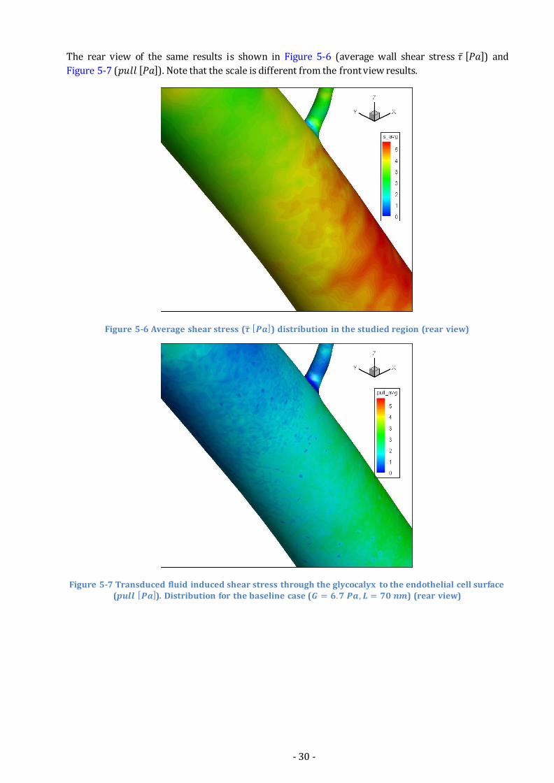
The rear view of the same results is shown in Figure 5-6 (average wall shear stress [ ]) and

Figure 5-7 ( [ ]). Note that the scale is different from the front view results.

Figure 5-6 Average shear stress ( [ ]) distribution in the studied region (rear view)

Figure 5-7 Transduced fluid induced shear stress through the glycocalyx to the endothelial cell surface ( [ ]). Distribution for the baseline case ( , ) (rear view)

- 31 -

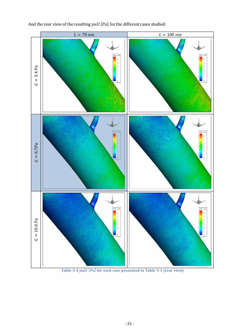
And the rear view of the resulting [ ] for the different cases studied:

Table 5-4 [ ] for each case presented in Table 5-1 (rear view)

- 32 -

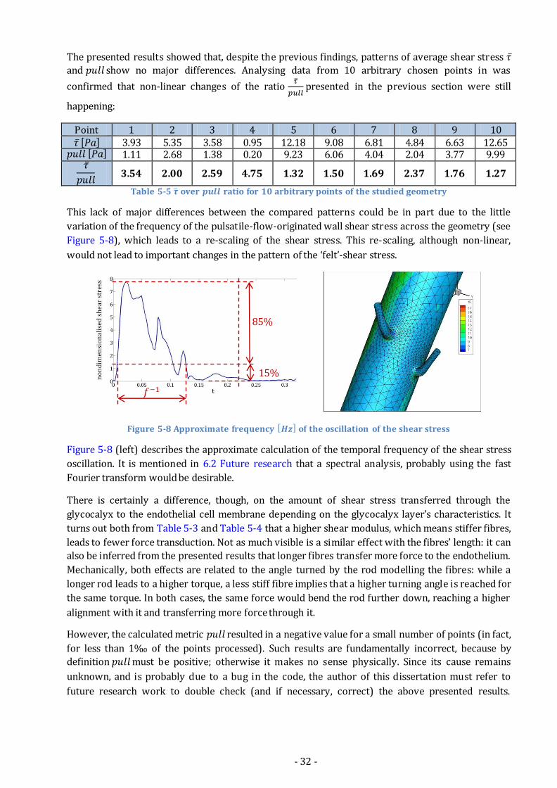
The presented results showed that, despite the previous findings, patterns of average shear stress

and show no major differences. Analysing data from 10 arbitrary chosen points in was

confirmed that non-linear changes of the ratio

presented in the previous section were still

happening:

Point 1 2 3 4 5 6 7 8 9 10 [ ] 3.93 5.35 3.58 0.95 12.18 9.08 6.81 4.84 6.63 12.65

[ ] 1.11 2.68 1.38 0.20 9.23 6.06 4.04 2.04 3.77 9.99

3.54 2.00 2.59 4.75 1.32 1.50 1.69 2.37 1.76 1.27

Table 5-5 over ratio for 10 arbitrary points of the studied geometry

This lack of major differences between the compared patterns could be in part due to the little

variation of the frequency of the pulsatile-flow-originated wall shear stress across the geometry (see

Figure 5-8), which leads to a re-scaling of the shear stress. This re-scaling, although non-linear,

would not lead to important changes in the pattern of the ‘felt’-shear stress.

Figure 5-8 Approximate frequency [ ] of the oscillation of the shear stress

Figure 5-8 (left) describes the approximate calculation of the temporal frequency of the shear stress

oscillation. It is mentioned in 6.2 Future research that a spectral analysis, probably using the fast

Fourier transform would be desirable.

There is certainly a difference, though, on the amount of shear stress transferred through the

glycocalyx to the endothelial cell membrane depending on the glycocalyx layer’s characteristics. It

turns out both from Table 5-3 and Table 5-4 that a higher shear modulus, which means stiffer fibres,

leads to fewer force transduction. Not as much visible is a similar effect with the fibres’ length: it can

also be inferred from the presented results that longer fibres transfer more force to the endothelium.

Mechanically, both effects are related to the angle turned by the rod modelling the fibres: while a

longer rod leads to a higher torque, a less stiff fibre implies that a higher turning angle is reached for

the same torque. In both cases, the same force would bend the rod further down, reaching a higher

alignment with it and transferring more force through it.

However, the calculated metric resulted in a negative value for a small number of points (in fact,

for less than 1‰ of the points processed). Such results are fundamentally incorrect, because by

definition must be positive; otherwise it makes no sense physically. Since its cause remains

unknown, and is probably due to a bug in the code, the author of this dissertation must refer to

future research work to double check (and if necessary, correct) the above presented results.

𝑓−

%

%

- 33 -

6 Conclusions and future research

6.1 Conclusions A mechanical model of the glycocalyx was developed in accordance with the literature on the matter.

For this model, the glycocalyx’ inertia was found to be negligible when compared to drag- and

stiffness-induced forces.

A convenient mathematical expression allowed defining, coding and checking a MATLAB algorithm

that calculated the glycocalyx’ response and a new metric called . This was defined, for a given

oscillating driving force, as the actual average pulling force transferred through the glycocalyx to the

endothelial cell surface. This new metric would then be compared to the average driving force (or

equivalently to the average shear stress ).

From the 1D analysis of idealised, sinusoidal driving forces it was concluded that for driving forces

with high amplitude, when compared to its average value, the oscillating frequency is a key, non-

linear factor when determining . This effect was increasingly important as the oscillating

frequency decreased, allowing the system to respond effectively to the higher amplitude.

The 1D mechanical model of the glycocalyx was appropriately extended to 2D in order to study

simulated shear stress data from a 3D geometry, corresponding to the descending thoracic aorta of a

rabbit. From the surface analysis of this large data set, comparing and , it was concluded that

although no major differences between the two metrics were observed, the glycocalyx does certainly

play a role in determining the amount of force transferred to the endothelium. Both higher length of

its fibres (a thicker cell-attached glycocalyx layer) and less stiff fibres resulted in higher amounts of

transduced force. It was also hypothesised that the lack homogeneity of shear stress oscillation

frequency across the geometry could cause the pattern of to be so similar to the ’s one.

6.2 Future research In the near future, the presented model could be double-checked and improved, although that would

probably lead to a model with increased complexity. Some of these next-steps are summarised

below:

As pointed out in 5.3 2D model results in the 3D geometry, a further check of the results with

special attention to the very few cases in which the calculated metric results in a negative

value is needed.

Given that the limitation in time of this project did not allow post-processing the entire set of

data available (see 5.3 2D model results in the 3D geometry), the first ‘next thing to do’ would be

it. That would also allow for a more in-depth analysis of the results and the importance of the

frequency response of the glycocalyx to the pulsatile blood flow.

It would be also desirable to present results as in Figure 1-2 (source: Vincent et al. [8]), for

which a ‘computational incision’ along the aortic wall to unwrap the geometry of the descending

aorta was made.

Solve the system of non-linear system of coupled differential equations with a different

approach: assuming the response’s oscillating frequency is the same as the perturbation’s

(driving force), it can be solved as a boundary values problem (BVP) instead of doing it as an

IVP. That might increase the solution’s accuracy. As mentioned in the Acknowledgements

section, another student in the Department of Aeronautics of Imperial College London is already

trying this new approach using University of Oxford’s chebfun solver for MATLAB.

The solving algorithms described in this dissertation have been coded in MATLAB and use this

software’s built-in solver ode45. However, the process takes a lot of time and in order to speed it

- 34 -

up, a wise option would be to code it in C++. Yet, that arises the problem of implementing a

differential equation solver which, although feasible (in fact I did so to check ode45’s accuracy

with the specific nonlinearity featured by the presented model), that would likely lead to a

decrease in accuracy. A different way to solve the model faster which was considered, but not

explored, would be using spectral methods.

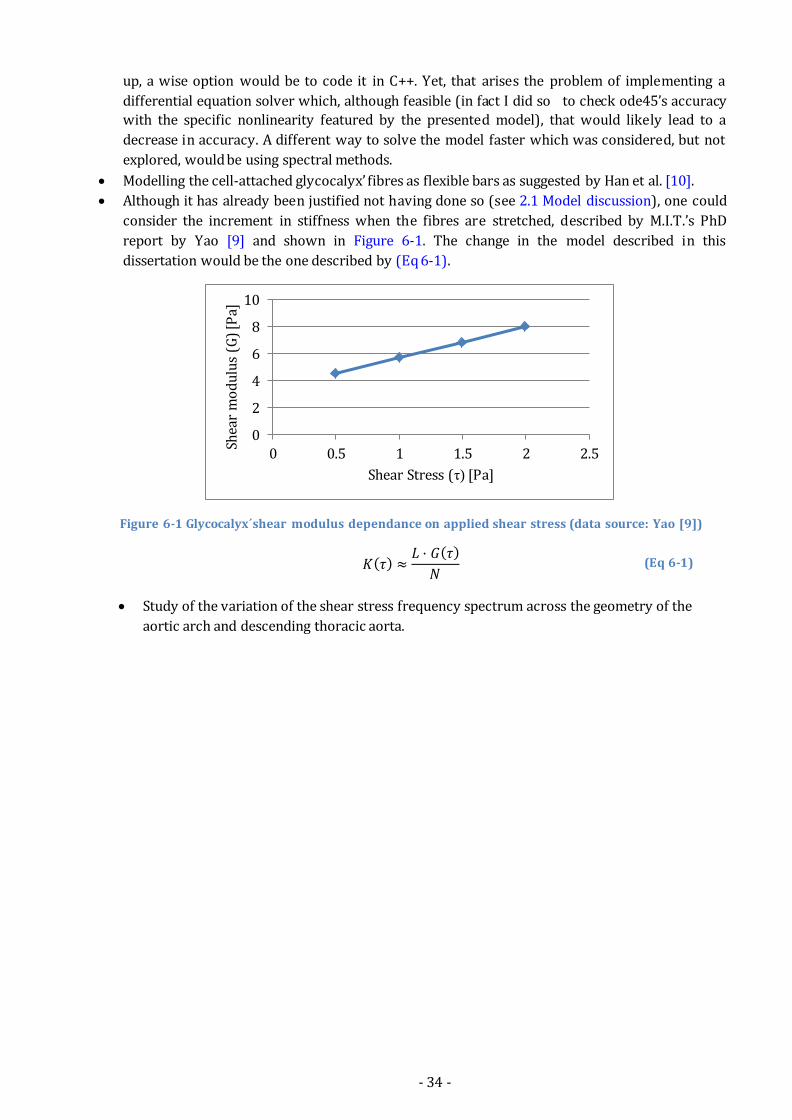
Modelling the cell-attached glycocalyx’ fibres as flexible bars as suggested by Han et al. [10].

Although it has already been justified not having done so (see 2.1 Model discussion), one could

consider the increment in stiffness when the fibres are stretched, described by M.I.T.’s PhD

report by Yao [9] and shown in Figure 6-1. The change in the model described in this

dissertation would be the one described by (Eq 6-1).

Figure 6-1 Glycocalyx´shear modulus dependance on applied shear stress (data source: Yao [9])

( ) ( )

(Eq 6-1)

Study of the variation of the shear stress frequency spectrum across the geometry of the

aortic arch and descending thoracic aorta.

0

2

4

6

8

10

0 0.5 1 1.5 2 2.5

Shea

r m

od

ulu

s (G

) [P

a]

Shear Stress (τ) [Pa]

- 35 -

Nomenclature 1 Introduction

Glycocalyx Endothelial Glycocalyx Layer, Endothelial Surface Layer BHF British Heart Foundation

2 The one dimensional model 1D One dimensional

( ) Second derivative ( )

( ) First derivative ( )

( ) Angle rotated down by the rod [ ] Inertia of the rod [ ]

Coefficient of rotational friction [

]

Rod’s mass [ ] Rod’s length [ ] Linear coordinate with the direction of the rod and origin at its articulation Drag force with respect to rotation [ ] Plasma viscosity [ ] Fibre radius [ ] Fibre volume fraction [ ] Darcy permeability of the glycocalyx [ ]

Fibre gap [ ]

Coefficient of a torsion spring [

]

Shear modulus [ ] Shear stress [ ]

Number of rods per area unit [

]

( ) Driving force applied on top of each rod [ ] Angular frequency [ ] Period [ ] Amplitude of the force [ ] Offset around which the force oscillates [ ] Non-dimensional time [ ] Non-dimensional frequency [ ] Non-dimensional period [ ] Non-dimensional amplitude [ ] Non-dimensional offset [ ]

IVP Initial Value Problem Initial condition ( ) [ ] Residual in the Manufactured Solutions Method [ ]

( ) Projection of the driving force in the direction of the rod [ ]

Tractioning ( ) integrated over a period [ ]. Its physical meaning

is the actual pulling force transferred through the glycocalyx to the endothelial cell surface

averaged over a period [ ] Ascending integer number (0, 1, 2…) [ ] Value of for which ( ) [ ]

Arbitrary value of for which ( ) has reached the steady state [ ] [ ] Interval of for which ( ) ( ) [ ]

- 36 -

4 The two dimensional model 2D Two dimensional Rod’s turned angle in xz-plane (from coordinate system A) [ ] Rod’s turned angle in yz-plane (from coordinate system A) [ ]

Rod’s turned angle in z-plane (from coordinate system B) [ ] Rod’s turned angle in xy-plane (from coordinate system B) [ ] Driving force in x direction [ ] Driving force in y’s direction [ ] Driving force in ’s direction [ ] Driving force in ’s orthogonal direction [ ]

Coefficient of rotational friction [

] for ’s rotation

Linear coordinate within the horizontal plane, origin in the z-axis and direction

Drag force with respect to rotation [ ]

( ) Vector representing magnitude and direction of a driving force at [ ]

( ) Vector of a ( ) set with maximum magnitude. Initial condition ( ) [ ] Initial condition ( ) [ ]

( ) orientation in coordinate

5 Study of simulated shear stress in a rabbit’s blood vessel Reference time (used in the nondimensionalisation) [ ]

Reference force (used in the nondimensionalisation) [ ]

Reference shear stress, equivalent to the reference fore ( ), (used in the nondimensionalisation) [ ]

6 Conclusions BVP Boundary Values Problem

- 37 -

Bibliography

[1] M. Nieuwdrop, M. C. Meuwese, H. L. Mooij, C. Ince, L. N. Broekhuizen, J. J. P. Kastelein and E. S. G.

Stries, “Measuring endothelial glycocalyx dimensions in humans: a potential novel tool to

monitor vascular vulnerability,” Journal of Applied Physiology, vol. 104, pp. 845-852, 2007.

[2] A. Pries, T. Secomb and P. Gaehtgens, “The endothelial surface Layer,” Pflügers Archiv European

Journal of Physiology, pp. 653-666, 2000.

[3] S. Reitsma, D. W. Slaaf, H. Vink, M. A. M. J. van Zandvoort and M. G. A. oude Egbrink, “The

endothelial glycocalyx: composition, functions, and visualization,” Pflügers Archiv European

Journal of Physiology, vol. 454, pp. 345-359, 2007.

[4] B. M. van den Berg, H. Vink and J. A. E. Spaan, “The Endothelial Glycocalyx Protects Against

Myocardial Edema,” Circulation Research, vol. 92, pp. 592-594, 2003.

[5] S. Weinbaum, X. Zhang, Y. Han, H. Vink and S. Cowin, “Mechanotransduction and flow across the

endothelial glycocalyx,” Proceedings of the National Academy of Sciences of the USA, vol. 100, no.

13, pp. 7988-7995, 2003.

[6] S. Weinbaum, J. M. Tarbell and E. R. Damiano, “The Structure and Function of the Endothelial

Glycocalyx Layer,” Annual Reviews, Boston, 2007.

[7] A. M. Shaaban and A. J. Duerinckx, “Wall Shear Stress and Early Atherosclerosis: A review,”

American Journal of Roentgenology, vol. 174, no. 6, pp. 1657-1665, 2000.

[8] P. E. Vincent, A. M. Plata, A. A. E. Hunt, P. D. Weinberg and S. J. Sherwin, “Blood flow in the rabbit

aortic arch and descending thoracic aorta,” J. R. Soc. Interface, pp. 1-12, 2011.

[9] Y. Yao, “Three-dimensional Flow-induced Dynamics of the Endothelial Surface Glycocalyx

Layer,” Massachusetts Institute of Technology, Boston, 2007.

[10] Y. Han, S. Weinbaum, J. A. E. Spaan and H. Vink, “Large-deformation analysis of the elastic recoil

of fibre layers in a Brinkman medium with application to the endothelial glycocalyx,” Journal of

Fluid Mechanics, vol. 554, pp. 217-235, 2006.

[11] T. Sadiq, S. Advani and R. Parnas, “Experimental investigation of transverse flow through aligned

cylinders,” International Journal of Multiphase Flow, vol. 21, no. 5, pp. 755-774, 1995.

[12] A. S. Sangani and A. Acrivos, “Slow flow thorugh a periodic array of spheres,” Int. J. Multiphase

Flow, vol. 8, no. 4, pp. 343-360, 1982.

[13] M. Haidekker, A. Tsai, T. Brady and H. Stevens, “A novel approach to blood plasma viscosity

measurement using fluorescent molecular rotors,” American Journal of Physiology, Heart and

Circulatory Physiology, vol. 282, p. H1609–H1614, 2002.

- 38 -

[14] F. E. Curry and R. H. Adamson, “Endothelial Glycocalyx: Permeability Barrier and

Mechanosensor,” Annals of Biomedical Engineering, vol. 40, no. 4, pp. 828-839, 2012.

[15] H. Luczak and W. Laurig, “An Analysis of Heart Rate Variability,” Ergonomics, vol. 16, no. 1, pp.

85-97, 1973.

[16] P. Vincent, “A Cellular Scale Study of Low Density Lipoprotein Concentration Polarisation in

Arteries,” Department of Aeronautics, Imperial College London, London, 2009.

[17] V. Peiffer, E. M. Rowland, S. G. Cremers, P. D. Weinberg and S. J. Sherwin, “Effect of aortic taper

on patterns of blood flow and wall shear stress in rabbits: Association with age,” Atherosclerosis,

vol. 223, no. 1, pp. 114-121, 2012.