Mechanical Quality Factor of Sapphire Membranes

Kane ScipioniUniversity of Florida

Università di Perugia / INFNUF IREU

August 10, 2010

Abstract

In the pursuit of ground-based gravitational wave detection, design of next generation detectors will need to consider many different limiting factors to their sensitivity that arise from improvements such as high powered lasers and monolithic suspension systems. One of these limiting factors is the thermal noise in the signal associated with the properties of the materials used to make the detector's mirrors. The high refractive mirror coatings are specifically the focus of understanding this noise. The purpose of this study is to see the behavior of specifically sapphire thin films, and the mechanical quality factor is a very good indicator of a material's ability to retain energy through oscillatory phenomena. Furthermore, this study includes a different technique to measuring the mechanical-Q that is alternative to cantilever driven oscillation. Sapphire could possibly be used as a replacement coating to tantalum pentoxide for future detectors, and is thus why the study of its mechanical-Q is of importance.

Introduction to Thermal Noise

Thermal noise is the excitation of charges in the lattice of a solid body due directly to the average thermal energy factor of the lattice constituents, kbT. This noise is created largely in part by the electrons in the material due to the stationary behavior of the positive ions in the lattice of a solid body. In mechanical measuring systems, such as a laser interferometer, these excitations interfere with the signals of very small oscillations of mechanical bodies, and thus limit the sensitivity of the interferometer. For future gravitational-wave detectors to operate with maximum sensitivity, the understanding of this noise in the materials of the test masses and knowing how to reduce it depends on relating the effects of thermal noise to mechanical oscillators in general. This can be done with the special case of Brownian motion of mechanical bodies, and the fluctuation-dissipation theorem is the most realistic approach to modeling the relationship between the power spectrum of thermal noise and the random forces that cause Brownian motion. A simple damped oscillator that works for this has the equation of motion

mx'' + ƒx' + kx = F

where ƒ is the damping coefficient of the dampening force, and k is the spring constant of the restoring force in the oscillator. According to Peter Saulson (1990) (et al.), the spectral density of the random thermal driving force as derived from the fluctuation-dissipation theorem can be expressed as

F2 = 4kbTR(ω)

with R(ω) as the mechanical resistance of the oscillator. Through Saulson's derivation of the admittance and solution of the system you obtain the complete position power spectrum of the mass in a damped oscillator system

x2(ω) = 4kbTƒ / [(k – mω2) + ƒ2ω2]

as a function of ω. This spectrum shows the relationship between the random motion of a body in a mechanically damped system and the thermal driving force. This relation manifests itself as the thermal noise spectrum. It is an important relation that shows us the behavior of this noise at different temperatures, masses, and frequencies. In the next section, we will see how the damped harmonic oscillator can show us the mechanical properties of systems that we wish to study, such as the coatings on interferometer mirrors.

The Quality Factor

The quality factor is a dimensionless quantity that measures the dampness of a mechanical system, or how long it takes a resonator to decay in amplitude. It is also the quantity of focus for this study of sapphire. Thus knowing the measurable properties that are related to the Q-factor, is of utmost importance. The most basic definition of Q is

Q = 2π * total energy of system / energy loss per cycle of oscillation

However, there are multiple ways of defining Q that are equivalent. Another being,

Q = f0 / Δf

where f0 is the resonant frequency of a system, and Δf is the bandwidth of the peak response at half the peak value. A third definition of Q is

Q = 1 / 2ζ

where ζ is the damping ratio for a damped harmonic oscillator. Because this is the particular system that is being studied, it is the definition that will be used in the calculation of Q for this experiment. The solution to the equation of motion for the damped oscillator is

x(t) = Ae-ζωt sin(√(1- ζ2) *ω0t + φ).

However, fitting this equation to the actual data would prove to be very difficult, and error prone. So, instead of doing this the measurement will be of the peak-to-peak amplitude of oscillation in very short intervals of time. This way the sinusoidal portion of the solution is approximately unity at these points and then only the exponential needs to be fitted to the data. This is convenient because the product of the damping ratio and the angular frequency of oscillation happens to equal the exponential attenuation. So it follows that

ζω0 = 1/τ

with τ being the time decay constant. With this it is easy to see that

Q = π f0τ

This relation is what is used to calculate the quality factor of the sapphire membranes in this study. The only quantity that needs to be measured is the time decay constant. The frequency of oscillation is controlled.

Typical Measurement of the Quality Factor

Typically the calculation of the Q-factor for thin films is done using a small film-coated silicon cantilever excited by an electrostatic drive. The fundamental resonant frequency of the cantilever is excited. Once the amplitude reaches its maximum, the drive is turned off and the decay of the peak-to-peak amplitude is recorded from a high sampling rate single-tone extractor. A Michelson interferometer is used to detect the decay of this amplitude, and the data from the photodetector is read by the tone extractor. A diagram of this setup is shown in the figure below (fig. 1). However, it is not a very simple process. The error in this kind of measurement is typically very high, and much care is needed to ensure that the cantilever is thermally and mechanically isolated. First, when this measurement is made, the Q that is actually calculated is the Q of the whole system, and not just the thin film. The energy losses due to the silicon, the clamping, and other various aspects of the apparatus contribute their properties to the Q. So to remedy this, the Q is measured before the cantilever has the film deposited on it, and then measured again after the physical vapor deposition. The energy losses are subtracted out using the loss angle of the components of the system. The loss angle is the inverse of the quality factor. It is a useful quantity because it is cumulative in nature, and can thus be subtracted out. However, during this process unclamping and reclamping of the cantilever can cause these losses to be different. As well, the physical vapor deposition can put stresses on the surface of the silicon changing this even when annealing has been preformed. So since this is a very delicate procedure, the experimental setup

for the study of sapphire membranes in this paper was slightly different. In the next section I will go over the setup used for this study.

fig.1 the typical setup for measuring Q

Experimental Procedure

vacuum chamber, sample, and interferometer

In this study, the sample films used were sapphire (Al2O3) membranes in the holes of a silicon substrate. The 0.5mm thick substrate had an array of 0.5mm diameter circular holes, in which after the deposition was performed, were the holes that the membranes stretched across. These membranes in particular were 92-96nm thick. This technique for mounting the sample eliminates the need to subtract out losses due to the silicon because the amplitude of oscillation being measured is that of just the membrane. Furthermore, the mounting system is extremely isolated by clamping a relatively very large substrate, and therefore the membranes were expected to not be significantly effected by the losses associated with the clamping. The interferometer optics were mounted in the vacuum chamber with the sample. One arm of the interferometer was used as a lever arm to be able to adjust the alignment of the laser beam as well as change the optical path on extremely small scales. A picomotor on one mirror and a piezoelectric motor on the other mirror of the lever arm were used to do this. The other arm, with the sample, has the beam aligned on one of the membranes, with the electrostatic drive pen mounted within 1mm on the other side of this membrane. The electrostatic drive is powered with a function generator signal from a high voltage amplifier. The beam size on the membrane was approximately 0.1mm, so the interferometer should be sensitive enough to detect the oscillations of the fundamental “drum-mode” of the sample. The 633nm 5mW laser and the photodetector were mounted outside the vacuum chamber, but inside a dark inclosure. A diagram of this experimental setup is shown below (fig. 2).

the control system

With the need for the interferometer to maintain its average intensity at the optimal operational point, a control system that uses feedback is required. In this particular system, the popular proportional-integral-derivative (PID) controller was used. The signal from the photodetector was sent through a

low-pass filter and preamplifier, with a cut-off frequency of 0.1Hz and a gain of 10. This signal, essentially as a DC offset, was sent to the DAQ, where the Labview feedback control VI collected data for the PID and made to corrections by adjusting the piezoelectric motor through a high-voltage piezoelectric amplifier. The operational point of the interferometer output was set to be at the middle between the highest average output and the lowest average output. Since the output of an interferometer behaves like a cosine-squared function with respect to optical path length, the desired operational point is in the linear region between the maximum and minimum average intensity. A DC offset was added to the piezoelectric amplifier to allow the motor to expand and contract with the PID.

the data acquisition

In this study, two different types of data acquisition were required for finding the preliminary frequency response (FRF) data and the decay oscillation of the membrane resonance. The FRF data was collected using the FFT analyzer. It acted as an oscilloscope for the raw signal from the photodetector on one input channel, and it took the output of the function generator on another input channel. The FFT analyzer creates a bode plot, and preforms averaging through a frequency sweep. The frequency sweep is preformed by the function generator, and then the FFT analyzer collects data on the system's response to the function generator's signal. This data is saved on to a 3.5” floppy disk. The FRF then reveals the resonance peak in the system. Now the function generator is set to drive the resonant frequency, and the amplitude decay data is taken. The raw signal is put through a hardware band-pass filter and preamplifier, to reduce the signal outside the realm of the frequency of oscillation. Then the signal goes to the DAQ where a second Labview VI is used to collect the data. Inside the Labview VI a DAQ assistant is used to sample the data, and the samples are sent through another band-pass filter. Then a waveform builder reconstructs the sinusoidal wave of the oscillation and sends this to a single-tone extractor. The extractor function outputs the frequency of the detected tone, and its peak-to-peak amplitude. The amplitude is the value that is collected for the exponential fitting. So, the exact procedure for obtaining this data starts with having the control system stabilized. The electric drive is turned on until the amplitude of the sample's oscillation is at a maximum. Then, the drive is turned off and the analytic data collection begins. The exponential fit is made, and the value of Q is calculated.

fig.2 the experimental setup

Results

The results I collected from this experiment did not exclusively include the time decay constants. As a matter of fact, the time decay ended up being the least important information I obtained. This is the case because the experiment was unable to detect a clean exponential decay. The analytic signal from the VI was extremely noisy, and every decay was just seen as a instantaneous drop in amplitude. I will discuss this later in this section in detail, as well as possible remedies. However, the most important information I obtained through the course of the experiment included the resonance mode modeling and the many frequency response functions.

resonance mode modeling

Using ANSYS Multiphysics, the range of resonant frequencies were calculated based on the geometry of the membranes, which were 0.5mm in diameter and 92-96nm thick. The upper and lower limits of possible thickness, Poisson ratio, and density variation. The range came to be between 6348Hz and 7475Hz. With this the range at which to search for resonance via a frequency sweep can be decided. This range was typically 6kHz to 8kHz during this experiment. Along with the value of the resonant frequency, the actual plots of average perpendicular displacement for each mode were printed. This is to ensure the mode being excited is the drum-mode of the sample, due to the interferometer sensitivity of this mode. However, during the initial data collection, the expected size of amplitude was not seen. In response, the next two circularly symmetrical modes were considered. In fact, near the center of the membrane ANSYS calculated a much larger average perpendicular displacement at these higher-order modes. The three plots of perpendicular displacement are shown below (fig. 3-5). The plots are of the frequencies 6865Hz, 26857Hz, and 60696Hz.

fig.3 average perpendicular displacement at 6865Hz

fig.4 average perpendicular displacement at 26857Hz

fig.5 average perpendicular displacement at 60696Hz

If the other modes were to be considered, the specifications of the high-voltage amplifier driving the sample needed to be checked. This is to ensure the response from the amplifier is full range. Instead it was found that the amplifier was out of specification during the initial data collections. The amplifier being used had a full scale cutoff at 2kHz and a low response cutoff at 5kHz. This was fixed very quickly by replacing it with another amplifier that had a full scale cutoff at 8kHz and low response at 35kHz. The effects of this change on the frequency response functions were relatively significant.

the frequency response function (FRF)

The FRF was the preliminary data that needs to be taken to know exactly what the resonance frequency of the sample is. The range of frequencies needed to be analyzed were determined by the ANSYS models. The calculated range was between 6kHz and 8kHz, so that is the range seen in the charts below (fig. 6-7). The frequency sweep done by the function generator was in 1 sec steps with 0.1Hz as the frequency stepping. In fig.6 the range was extended down to 4kHz as a comparison to show the activity of the resonance in the upper range. Also in this figure, the black and red plots show the first two FRF collected, and the green shows the third FRF collected. This was done to ensure the consistency of behavior in the system. This data was collected with the previously used amplifier, and therefore the response from the resonance was relatively smaller than it should be. Other peaks were relativity larger than they were supposed to be, so all of the peak frequencies were excited to see the response. This method was used until the amplifier was changed. The higher response amplifier produced the FRF seen in fig.7. In this figure the response of the resonance is much more obvious. Its frequency was around 6562Hz. However, The actual response in the analytic signal from the tone extractor, was still minimal.

fig. 6 frequency response function 6kHz to 8kHz, and 4kHz to 6kHz

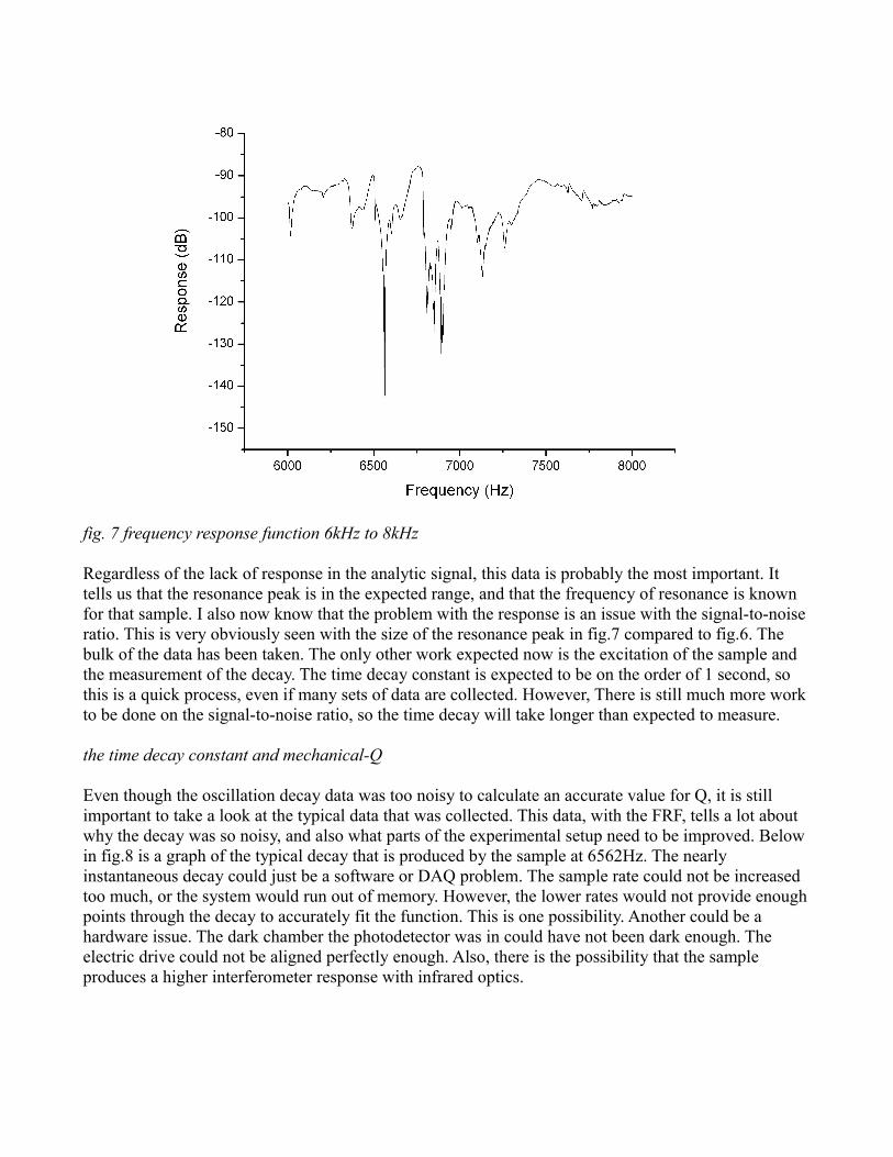
fig. 7 frequency response function 6kHz to 8kHz

Regardless of the lack of response in the analytic signal, this data is probably the most important. It tells us that the resonance peak is in the expected range, and that the frequency of resonance is known for that sample. I also now know that the problem with the response is an issue with the signal-to-noise ratio. This is very obviously seen with the size of the resonance peak in fig.7 compared to fig.6. The bulk of the data has been taken. The only other work expected now is the excitation of the sample and the measurement of the decay. The time decay constant is expected to be on the order of 1 second, so this is a quick process, even if many sets of data are collected. However, There is still much more work to be done on the signal-to-noise ratio, so the time decay will take longer than expected to measure.

the time decay constant and mechanical-Q

Even though the oscillation decay data was too noisy to calculate an accurate value for Q, it is still important to take a look at the typical data that was collected. This data, with the FRF, tells a lot about why the decay was so noisy, and also what parts of the experimental setup need to be improved. Below in fig.8 is a graph of the typical decay that is produced by the sample at 6562Hz. The nearly instantaneous decay could just be a software or DAQ problem. The sample rate could not be increased too much, or the system would run out of memory. However, the lower rates would not provide enough points through the decay to accurately fit the function. This is one possibility. Another could be a hardware issue. The dark chamber the photodetector was in could have not been dark enough. The electric drive could not be aligned perfectly enough. Also, there is the possibility that the sample produces a higher interferometer response with infrared optics.

fig. 8 the noisy decay of the sample membrane oscillation

conclusion

The minimal response in the analytic signal is the limiting factor for finding the mechanical-Q of these sapphire membranes. The measurement is very difficult due to the geometry of the samples being 0.5mm diameter circular films. When the decay is accurately measured, though, the other arbitrary losses are much lower than when using a cantilever experiment. I propose that with a few improvements we will see a higher response in the system, and thus the response in the amplitude of oscillation will be collected with less noise. One improvement that is particularly important is the alignment of the electric drive. Since it is what excites the resonant mode, it needs to do so with the highest efficiency possible. With the electric drive pen attached to a picomotor, the pen can be nearly perfectly aligned in the center of the membrane as well as perfectly perpendicular to the plane of the film. This I believe was not possible to obtain using alignment by hand. Improvements in the isolation of the photodetector from the ambient light would be beneficial. The dark chamber could possibly have let light that distorts the signal in the chamber. This is especially so when using visible light laser beams. One last improvement is to change all the optics to infrared. This would be a complete over haul of the experimental setup. If it is possible to align the beam correctly with an infrared laser, the membranes may produce a stronger signal for the photodetector. However, the other options for improvement should be explored first, as this is just a hypothesis.

Sources

Cagnoli G, Gammaitoni L, Hough J, Kovalik J, McIntosh S, Punturo M, Rowen S, Very High Q “Measurements on a fused Silica Monolithic Pendulum for Use in Enhanced Gravity Wave Detectors”, 2000, Physical Review Letters, vol 85, #12

Levin, Yur'evich, “Internal thermal noise in the LIGO test masses: A direct approach”, 1998, Physical Review D, vol 57, #2

Martin I, Armandula H, Comtet C, Fejer M, Gretarsson A, Harry G, Hough J, Mackoski J, MacLaren I, Michel C, Montorio J, Morgado N, Nawrodt R, Penn S, Reid S, Remillieux A, Route R, Rowan S, Schwarz C, Seidel P, Vodel W, Zimmer A, “Measurements of a low-temperature mechanical dissipation peak in a single layer of Ta2O5 doped with TiO2”, 2008, IOP publishing, Classical and Quantum Gravity, vol 25

Mattox, Donald, “The Foundations of Vacuum Coating Technology”, 2003, William Andrew Publishing

Numata K, Otsuka S, Ando M, Tsubono K, “Intrinsic losses in various kends of fused silica”, 2002, IOP, Classical and Quantum Gravity, vol 19, 1697-1702

Saulson, Peter, “Thermal noise in mechanical experiments”, 1990, Physical Review D, vol 42, #8

Zener, Clarence, “Internal Friction in Solids”, 1937, Physical Review, vol 52, 230-235