MECHANICAL PERFORMANCE OF V-RIBBED BELT DRIVES

MECHANICAL PERFORMANCE OF

V-RIBBED BELT DRIVES

Seyed Mohammad Tabatabaei Lotfy

A thesis submitted in accordance with the requirements

for the degree of Doctor of Philosophy

The University of Leeds

Department of Mechanical Engineering

April 1996

(The candidate confirms that the work submitted is his own and that appropriate)

(credit has been given where reference has been made to the work of others)

ABSTRACT

The design and shape of a v-ribbed belt affects its radial movement in the pulley

. _._,grooves. When rib bottom I groove tip contact occurs the wedge action decreaSes ... :-,-.....;~,

The beginning of the contact depends on belt tension, fit between rib and groove,

wear and material properties.

For the first time a non-contact laser displacement meter has been used for

dynamic measurements of the radial movement of a v-ribbed belt (type 3PK) around

the arc of wrap running on a belt testing rig. Accurate and repeatable results are

possible. By the help of this device, the radial movement and the beginning of the rib

bottom I groove tip contact around the arc of wrap ha.ve been determined

experimentally for tested v-ribbed belts. This point plays an important role in the

mechanical performance of v-ribbed belt drives.

Two sizes of standard pulleys were used for mechanical testing. These were paired with nominal effective diameters, de =45 mm and de =80 mm. Tests were

carried out at the speed of c.o =2000 RPM and two different values of total belt tensions (F, + F,.) for three different types of rib bottom I groove tip contact.

(i) Without contact

(ii) With contact

(iii) Mixed contact

Slip, torque loss and maximum torque capacity have been measured

experimentally during the tests.

A v-ribbed belt is assumed to be a combination of a flat belt and a v-belt with the

same radial movement of the two parts. Based on these assumptions a new theory is

developed for the mechanical performance of v-ribbed belt drives, which gives a new

modification to Euler's equation (capstan formula). By the help of Maple V

(mathematical standard library software) numerical solutions for theoretical modelling

give the variation of non-dimensional values of v-ribbed belt tension, flat belt part of

v-ribbed belt tension, v-belt part of v-ribbed belt tension, radial movement and sliding

angle with the length of active arc. This theory has been developed to obtain

expressions for speed loss (slip) in linear and non-linear zones.

The experimental and theoretical results show that the radial movement and slip of

the v-ribbed belt with rib bottom I groove tip contact is slightly less than the values

without contact. However, in spite of more or less apparent similar performance of v

ribbed belt wi~ and without rib bottom contact, it is found experimentally and'

theoretically that the compressed rubber of the belt (between cord and pulley) is

subjected to a variable internal shear force around the pulley after contact~

Acknowledgement

.. The author wishes to express his sincere gratitude to his supervisor Prof. T. H. C.

Childs for his assistance, guidance and encouragement throughout this work.

Thanks are also due to superb technical assistance provided by the staff of the

Department of Mechanical Engineering and all the friends in the department for their

support and assistance.

The financial support by the Islamic Republic of Iran, specially Ministry of Culture

and Higher Education and Ministry of Education and Training, is gratefully

acknowledged.

Finally, the author wishes to express his utmost appreciation to his wife and

children for their support and patience during this work.

In the name of God

To my parents

and

my family

Table of Contents

List of Tables

List of Figures

List of Symbols

Chapter One:

Chapter Two:

Table of Contents

Introduction

Belt Drives (Literature Review)

2.1 Introduction

2.2 Flat Belt Drives

2.2.1 Classical Theory

2.2.2 Different Mechanisms of Speed Loss

2.2.2.1 Belt extension

2.2.2.2 Rubber compliance

2.2.2.3 Shear deflection

2.2.2.4 Seating and unseating

2.2.3 Torque Loss

2.3 V-belt Drives


2.3.2 Radial Movement

2.3.3 Gerbert's V-belt Theory

2.3.3.1 Gerbert's Contribution to Radial

Movement

2.3.3.2 V-belt Equations Solution

2.3.3.3 Non-Linear Slip

2.3.4 Torque Loss

2.4 V-ribbed Belt Drives

i

v

vii

xii

1

4

4

6

6

8

8

8

9

10

11

12

12

12

15

18

22·

28

30

31

ii

2.4.1 Torque Capacity 33

2.4.2 V -ribbed Belt Slip 34

2.4.3 Gerbert's V-ribbed Theory 37

2.4.4 V -ribbed Belt Torque Loss 43

2.4.5 Development of V -ribbed Belt in This Thesis 43

Chapter Three: V -ribbed Belt Theory 44

3.1 Introduction 44

3.2 Equilibrium Equations 46

3.3 Radial Movement 47

3.3.1 Radial Movement of V -belt Part 48

3.3.2 Radial Movement of Flat Belt Part 52

3.4 Basic Equations 53

3.4.1 V -ribbed Belt Equations ·Solution 56

3.4.2 Non-Linear Slip 68

Chapter Four: Belt Testing Rig and Instrumentation 72

4.1 Introduction 72

4.2 Dynamometer 73

4.3 Instrumentation of Dynamometer 75

4.3.1 Non-Contact Laser Displacement Meter 75

4.3.2 Speed Measurements 76

4.3.3 Torque Measurements 76

4.4 Rig Calibration 78

4.4.1 Radial Movement 79

4.4.2 Slip Calibration 80

4.4.3 Torque Calibration 81

4.4.4 Total Tension Calibration 85·

Chapter Five: V -ribbed Belt Material Properties 86

5.1 Introduction 86

5.2 Radial Spring Constants 91

Chapter Six:

iii

5.2.1 Preliminary Test 91

5.2.2 Tests For Determination of Radial Spring 92

,,_.:.Constant kv

5.2.3 Tests For Determination of Radial Spring 96

Constant kF

5.3 Coefficient of Friction 98

5.3.1 Introduction 98

5.3.2 Coefficient of Friction for V-ribbed Belts 99

5.3.3 Measurements Methods 100

5.4 Extension Modulus, c 102

Experimental Investigation of

V -ribbed Belt Performance

104

6.1 Introduction 104

6.2 Experimental Method 105

6.3 Fundamental Experiments 109

6.3.1 Radial Movement 109

6.3.2 Slip and Torque Loss 121

6.3.3 Subsidiary Tests for Slip and Torque Loss 125

Chapter Seven: Discussion of the Experimental 140 ,

and Theoretical Results

7.1 Introduction 140

7.2 Radial Movement 141

7.2.1 Experimental Results 141

7.2.2 Theoretical Non-Skidding Condition Results 144

7.2.3 Theoretical Skidding Condition Results 144

7.2.4 Mixed Contact 146-

7.2.5 Discussion of Results 156

7.3 Slip 159

7.4 Maximum Traction 164

iv

7.5 Torque Loss and Efficiency 167

7.6 Is the V-ribbed Belt a V-belt or Flat Belt? 169

Chapter Eight: Conclusions and Recommendations for Future Work 174

References

Appendix (A)

Appendix (B)

Appendix (C)

Appendix (D)

8.1 Conclusions 174

8.2 Recommendations for Future Work 176

178

186

191

192

196

v

List of Tables

Table 2.1 Numerical results for Gerbert's equations (driven pulley) 26

Table 2.2 Numerical results for Gerbert's equations (driving pulley) 27

Table 3.1 Numerical results for v-ribbed belt equation (driven pulley) 70

Table 3.2 Numerical results for v-ribbed belt equation (driving pulley) 71

Table 4.1 Pulley diameter measurements 81

Table 4.2 Experimental results for linearity between digital units 83

and applied torque

Table 4.3 Experimental results for windage calibration 84

Table 5.1 Sheave or pulley groove dimensions for v-ribbed belts 88

Table 5.2 Tests for the variation of HT across the belt' width at 92

angular position 90 degrees

Table 5.3 Tests for determination of kv 95

Table 5.4 Tests for determination of kF 97

Table 6.1 Range of variables in mechanical tests 107

Table 6.2 The amount of wear during each set of tests 109

Table 6.3 Experimental readings of H T (mm), for (F, + F; =200 N, de =45mm) 129

Table 6.4 Experimental readings of HT (mm), for (F, +F;=300 N, de =45mm) 130

Table 6.5 Experimental readings of H T (mm), for (F, + F; =200 N, de =80mm) 131

Table 6.6 Experimental readings of HT (mm), for (F, + F; =600 N, 132, 133

de=80mm)

Table 6.7 Experimentalreadings of HT (mm), for (F, +F;=600 N, de =45mm) 134

Table 6.8 Experimental data for slip and torque loss, de=45mm 135

Table 6.9 Experimental data for slip and torque loss, de =80mm 136

vi

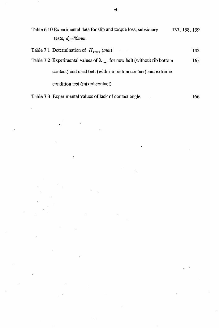
Table 6.10 Experimental data for slip and torque loss, subsidiary

tests, de =80mm

137, 138, 139

Table 7.1 Determination of HTmax (mm) 143

Table 7.2 Experimental values of "'max for new belt (without rib bottom 165

contact) and used belt (with rib bottom contact) and extreme

condition test (mixed contact)

Table 7.3 Experimental values of lack of contact angle 166

vii

List of Figures , . ~;' "'~' . ~

Fig. 2.1 Typical view of a belt drive 5

Fig.2.2 Flat belt power transmission (driving pulley) 7

Fig. 2.3 Tension variation for driving pulley 11

Fig.2.4 An exaggerated view of a v-belt drive 14

Fig. 2.5 Defining the sliding angle 'Y 14

Fig. 2.6 Forces acting on a v-belt element 17

Fig. 2.7 Belt wedge angle at the sliding angle 17

Fig. 2.8 Three sources of belt deformation allowing radial movement . 19

Fig.2.9 Perpendicular forces acting on a belt cross-section 19

Fig. 2.10 Solution to Gerbert's equations for driven pulley 24

Fig. 2.11 Solution to Gerbert's equations for driving pulley 25 Fig. 2.12 Theoretical relation between F I F, and <p for 29

matching real and fictitious system

Fig. 2.13 Theoretical slip sc I (F, + F,.) as a function of traction coefficient 29

Fig. 2.14 Cross-section of a K-section v-ribbed belt (dimensions mm) 32

Fig. 2.15 The slip as a function of transmitted torque in a v-ribbed belt 34

Fig. 2.16 Experimental slip quantity ( c . tloo) vs coefficient 36 F,+F,. 0)

of traction A. for different total tension (F, + F,.),

(v-ribbed belt). Comparison with "classical" flat belt theory

Fig. 2.17 Theoretical slip quantity ( c . tloo) vs coefficient 36 F,+F,. 0)

of traction A. for different total tension (F, + F,.), (v-ribbed belt)

Fig. 2.18 Wedge load Pv and bottom load PF of the rib 38

Fig. 2.19 Defining the mechanism of rib bottom I groove tip contact 42

Fig. 3.1 Flat belt part and v-belt part of a v-ribbed belt load 45

Fig.3.2 Forces acting on a v-ribbed element 46·

Fig.3.3 Perpendicular forces acting on a v-ribbed belt cross-section 47

Fig.3.4 Geometry of radial movement and axial strain 49 Fig.3.5 Solution to v-ribbed belt theory for driven pulley (de=45mm) 62

viii

Fig.3.6 Solution to v-ribbed belt theory for driven pulley (de =80mm)

Fig.3.7 Solution to v-ribbed belt theory for driving pulley (de =45mm)

Fig. 3.8· Solution to v-ribbed belt theory for driven pulley (de =80mm)

63

64

65

Fig. 3.9 Variation of belt tractions of flat and v- belt parts ·of a v-ribbed 66

belt against active arc for driven pulley

Fig. 3.10 Variation of belt tractions of flat and v- belt parts of a v-ribbed 66

belt against· active arc for driving pulley

Fig. 3.11 Variation of belt normal load of flat and v- belt parts of a v-ribbed 67


Fig. 3.12 Variation of belt tractions of flat and v- belt parts of a v-ribbed 67


Fig. 3.13 Theoretical slip sc I (F, + F,) as a function of traction coefficient 68

Fig. 4.1 Schematic of the belt testing rig 74

Fig.4.2 Schematic of the non-contact laser displacement meter 76

Fig 4.3 Configuration of laser sensor head stand and speed 77

measurement arrangements

Fig. 4.4 Determination of pitch diameter

Fig. 4.5 Response between transducer and digital output

Fig. 4.6 Windage resistance against speed

Fig. 5.1 Fully molded v-ribbed belt construction

Fig.5.2 V-ribbed belt with ribs formed by grinding

Fig. 5.3 Standard groove dimensions

Fig. 5.4 The variation of radius Rr against belt tension F, for a

new v-ribbed belt

79

82

84

87

87

89

95

Fig. 5.5 The variation of radius Rr against belt tension F, for a 97

used v-ribbed belt

Fig. 5.6 Test rig for coefficient of friction measurements 102

Fig.6.1 Variation of drive radius and radial movement against angular 112

position for a new v-ribbed belt (without rib bottom contact)

(F,+F,=200N, de=45mm)

Fig.6.2 Variation of drive radius and radial movement against angular 113

position for a used v-ribbed belt (with rib bottom contact)

(F, + F,=200 N, de =45 mm)

ix

Fig. 6.3 Variation of drive radius and radial movement against angular 114


(F, + F, =300 N, de =45 mm)



(F,+F,=300N, de=45mm)


position for a new v-ribbed belt (without rib bottom conta<?t)

(F, + F,=200 N, de =80 mm)



(F, + F, =200 N, de =80 mm)



(F, + F, =600 N, de =80 mm)



(F, +F,=600N, de=80mm)

Fig. 6.9 Variation of drive radius and radial movement agains~ angular 120

position for a new v-ribbed belt (extreme conditions

test with mixed contact) (F, + F, =600 N, de =45 mm)

Fig. 6.10 Slip (s) verses (F, - F,.) for new (without rib bottom contact) 128

and used (with rib bottom contact) v-ribbed belts and extreme

conditions test (mixed contact) (de =45mm)

Fig. 6.11 Slip (s) verses (F, - F,.) for new (without rib bottom contact) 128

and used (with rib bottom contact) v-ribbed belts (de=80mm)

Fig. 6.12 Torque loss (TL ) verses (F, - F,.) for new 130

(without rib bottom contact) and used (with rib bottom contact)

v-ribbed ~elts (de =45mm) , (a) F, + F,.=200 N, (b) F, +F,.=300 N,

(c) extreme conditions test, F, + F,. =600 N

Fig. 6.13 Torque loss (TL ) verses (F, - F,.) for new (without rib bottom contact) 131

and used (with rib bottom contact) v-ribbed belts (de =80mm),

x

(a) F, + F,.=200 N, (b) F, + F,.=600 N

Fig. 6.14 Slip (s) verses (F, - F,.) for (a) new, half-used and used cut belts 133

(b) new cut, new molded and new anti-wear belts (c) new cut,

0)~1000 RPM and 0)=2000 RPM (de =80mm, F, + F,. =470 N)

Fig. 6.15 Torque loss verses (F, - F,.) for (a) new, half-used and used belts 134

(b) cut, molded and anti-wear belts (c) 0)=1000 RPM,

0)=2000 RPM (de =80mm, F, + F,. =470 N)

Fig.7.1 Experimental and theoretical results of radial movement against 147

angular position for v-ribbed belt with rib bottom I groove tip contact

(used belt) and without contact (new belt), (de =45mm,

F, + F,. =200N.m, non-skidding condition, Torque =2.5N.m)

Fig. 7.2 Experimental and theoretical results of radial movement against 148



F, + F,.=200N.m, skidding condition, Torque =4N.m)



(used belt) and without contact (new belt), (de=45mm,

F, + F,. =300N.m, non-skidding condition, Torque =2.5N.m)




F, + F,. =300N.m, skidding condition, Torque =6N.m)



(used belt) and without contact (new belt), (de=80mm,

F, + F,.=200N.m, non-skidding condition, Torque =5N.m)

Fig.7.6 Experimental and theoretical results of radial movement against 152·




xi

Fig.7.7 Experimental and theoretical results of radial movement against 153

angular position for v-ribbed belt with rib bottom / groove tip contact


F, +F,.=600N.m, non-skidding condition, Torque =10N.m)

Fig.7.8 Experimental and theoretical results of radial movement against 154·

angular position for v-ribbed belt with rib bottom / groove tip contact



Fig. 7.9 Experimental and .theoretical results of radial movement against 155

angular position for v-ribbed belt (extreme conditions test) with mixed

rib bottom / groove tip contact (de =45mm, F, + F,. =600N.m,

skidding condition, Torque =13N.m)

Fig. 7.10 Variation of FIR against HT' for a new v-ribbed belt or

without rib bottom / groove tip contact (data from table 5.3)

Fig.7.11 Variation of FIR against HT' for a used v-ribbed belt or 158

with rib bottom / groove tip contact (data from table 5.4)

Fig. 7.12 Experimental, theoretical and semi-theoretical slip (s . c) / (F, +F,.) 162

as a function of traction coefficient (de =45mm)

Fig. 7.13 Experimental, theoretical and semi-theoretical slip (s ·c) / (F, + F,.) 163

as a function of traction coefficient (de =80mm)

Fig. 7.14 Efficiency versus transmitted torque for new, half-used, used, 168

molded, anti-wear v-ribbed belt (00=1000 RPM and 00=2000 RPM)

xii

List of Symbols

B Belt pitch

E Young's modulus

F Belt tension

H Total belt depth

HT Radial belt depth (Fig. 4.4)

P Input power

PL Power loss

R Pitch radius of belt

Re Pulley effective radius (outside Radius)

Rea Pulley actual effective radius

Rr Pulley radius over top of belt (Rr=HT+Rea)

T Input torque

TL Torque loss

T Traction force per unit length

V Belt tension member speed

c Belt extension modulus (F=CE)

de Pulley nominal effective diameter

dea Pulley actual effective diameter

k Spring constant

p

s

x

r

A.

S

fl

xiii

Axial spring constant

Radial spring constant

Longitudinal spring constant

Radial spring constant of flat belt part of a v-ribbed belt

Radial spring constant of v-belt part of a v-ribbed belt

Total spring constant of v-ribbed belt (kYR=ky+kF)

Groove pressure (force per unit length)

Normal force per unit length

Slip factor

Radial movement

Arc of wrap

Angular position

Half angle of pulley groove

Belt half wedge angle at sliding angle (Fig. 2.7)

Longitudinal strain

Angular co-ordinate (active arc)

Length of arc of wrap with rib bottom I groove tip contact (Fig. 2.19)

Length of arc of wrap without rib bottom I groove tip contact (Fig.

2.19)

Sliding angle

Coefficient of traction (A. = F, - F, I F, + F,)

Inclination of belt in groove

Coefficient of friction

v

(0

Indices

F

V

dg

dn

g

m

r

t

w

X,Y,z

xiv

Poisson's ratio

Angular speed

Flat belt of a v-ribbed belt

V -belt part of a v-ribbed belt

Driving pulley

Driven pulley

Generator

Motor

Relax (slack) side

Tight side

Windage

Radial, circumferential (longitudinal) and axial directions

CHAPTER ONE

INTRODUCTION

Belt drives have played an important role in the industrial development of the

world for more than 200 years. They are used as a means of transmitting power by

frictional forces developed between the belt and the pulley. Belt drives are used in a

wide range of power transmissions due to their advantages such as low maintenance

cost, quiet operation, low initial cost and fairly efficient operation (usually 95% for v

and v-ribbed belt drives).

In 1917 John Gates'developed the first rubber v-belt to replace the round hemp

rope used to drive the fan on a 1917 Cole coupe'. V-belts through wedge action,

increased the frictional force between the belt and the pulley for the same coefficient

of friction. This gave the v-belt a very fast rise in popularity within a few years.

The v-ribbed belt was introduced in the 1950s. It is a cross between a flat and a

v-belt. This belt is essentially a flat belt with v-shaped ribs projecting from the bottom

of the belt which guides the belt and make it more stable than a flat belt. In the

original concept, the v-ribs of the belt completely filled the grooves of the pulley. For

this reason, the v-ribbed belt did not have the wedging action of the. v-belt and

2

consequently had to operate at higher belt tensions. Later versions of v-ribbed belts

have truncated ribs to more closely emulate the wedging effect of a v-belt [1,29].

,,<,._~",~"" " . "~'·lT''''''''".',u.,~''1''- ,._ .... ,

The design· and shape of a v-ribbed belt affects its radial movement in the pulley

grooves. When rib bottom I groove tip contact occurs the wedge action decreases.

The beginning of the contact depends on belt tension, fit between rib and groove,

wear and material properties. Therefore it is not obvious if a v-ribbed belt functions

as a v-belt or a flat belt. The purpose of this work was to investigate theoretically and

experimentally the factors that influence the mechanical performance of v-ribbed belt

drives. Investigating the mechanical performance of v-ribbed belt drives requires a

clear idea to be developed on radial movement of the v-ribbed belt and its effect on

the other parameters of the mechanism.

Chapter two gives a literature review on v-ribbed belt drives and elements of

theory from flat and v-belt drives related to v-ribbed belt mechanical performance.

In chapter three on belt theory, a v-ribbed belt is assumed to be a combination of a

flat belt and a v-belt with the same radial movement of the two parts. Based on these

assumptions a new theory is developed for the mechanical performance of v-ribbed

belt drives, which gives a new modification to Euler's equation (capstan formula). By

the help of Maple V (mathematical standard library software) numerical solutions for

theoretical modelling give the variation of non-dimensional values of v-ribbed belt

tension, flat belt part of v-ribbed belt tension, v-belt part of v-ribbed belt tension,

radial movement and sliding angle with the length of active arc. This theory has been

developed to obtain expressions for speed loss (slip) in linear and non-linear zones.

Chapter four describes a test rig and its instrumentation to measure the values of

. radial movement, speed and torque losses.

For the first time a non-contact laser displacement meter has been used for'

dynamic measurements of the radial movement of a v-ribbed belt (type 3PK) around

the arc of wrap running on a belt testing rig. Accurate and repeatable results are

3

possible. By the help of this device, the radial movement and the beginning of the rib

bottom I groove tip contact around the arc of wrap have been determined

experimentally for tested v-ribbed belts. This point'pra.)rs'aniiriportant role in the

mechanical performance of v-ribbed belt drives.

Material properties of v-ribbed belts required in the theoretical modelling have

been measured experimentally in chapter five.

Experimental results of the tests carried out are given in chapter six. Two sizes of

standard pulleys were used for mechanical testing. These were paired with nominal

effective diameters, de =45 mm and de =80 mm. Tests were carried out at the speed of

0>=2000 RPM and two different values of total belt tensions (F, + F,) for three

different types of rib bottom I groove tip contact.

(i) Without contact

(ii) With contact

(iii) Mixed contact

Slip, torque loss and maximum torque capacity have been measured

experimentally during the tests.

The experimental and theoretical results are compared and discussed in chapter

seven. The results show that the radial movement and slip of the v-ribbed belt with

rib bottom I groove tip contact is slightly less than the values without contact.

However, in spite of more or less apparent similar performance of v-ribbed belt with

and without contact, it is found experimentally and theoretically that he compressed

rubber of the belt (between cord and pulley) is subjected to a variable internal shear

force around the pulley after contact.

Chapter eight summarises the major findings of the work and makes,

recommendations for future programmes of research in this and related areas.

4

CHAPTER TWO

BELT DRIVES

(Literature Review)

2.1 Introduction

This chapter will review v-ribbed belt drive literature and elements of theory

from flat and v-belt drives related to v-ribbed belt mechanical performance. In this

work special attention will be made to radial movement and its contribution to the

slip and speed loss. There will also be a brief review of torque loss contribution to

power loss.

When a belt drive is transmitting power, the strand tensions are not equal. There is

a tight side tension F, and a slack side tension F, and difference between these

tensions is often called the effective tension or net pull. This is the force that

produces work, and the rate at which work is performed is called power.

In Fig. 2.1 a typical view of a belt drive with two pulleys is shown. The pulleys are

taken to be rotating clockwise. The belt is represented as a band by its cord line. The,

driving pulley is denoted dg and the driven pulley dn. The drive consists of two

pulleys with pitch radius R.

5

When torque is applied to the system, the input power to the driving pulley is

given by (0) Ddg where 0) is the angular speed and T is the torque on the pulley. The

output power from the driven pulley is (0) D dn , Their difference is'the power loss PL

in the drive.

For pulleys of equal size the power loss may be written

Dividing by the input power P we have the fractional power loss

PL =s+ TL P T

where

(2.1)

(2.2)

(2.3)

In a belt drive the slip s and the fractional torque loss TL I T result from several

effects [1].

Driven pulley Driving pulley

Fig. 2.1 Typical view of a belt drive

./

6

2.2 Flat Belt Drives

It is appropriate to review flat belt theory as some aspects are related to v-ribbed

belt drives.


The role of friction in the equilibrium of ropes wrapped around shafts was

analysed by Euler [2]. He presented the well-known capstan formula, which relates

the slack and tight tensions of a rope to the friction coefficient J.1 and angle of wrap

of the rope on the pulley a.

F -' =exp(J.1a) Fr

(2.4)

According to Gerbert [3], this theory was applied to flat and v-belt drives by

Eytelwein [4]. The angle a was taken as the geometrical angle of wrap. Norman [5]

recognised that stiffness in the belt causes arching in the strands between the pulleys

and reduces the arc of contact between belt and pulley. More comprehensive theory

was given by Hornung [6]. The lack of contact angle reduces the maximum traction

of the drive [1].

When equation (2.4) is satisfied and skidding occurs, the fractional speed loss s

tends to 1.0. A smaller tension ratio than in equation (2.4) requires a sliding arc <P s

(active or sliding arc) obtained from

F ; = exp(J.1<p s)

r

<P s is located towards the exit region (Fig. 2.2). In this region belt tension F is given

by (for a driving pulley)

F F = exp(J.1<p) r

<P is the angular co-ordinate and Fr is the tension at <P =0. If the geometric contact

arc is a there is no sliding and no friction within the arc epa =a-<ps (adhesion or

7

idle arc). At this region the belt force remains constant [7]. The size of the active arc

is dependent on (F, - Fr) .

F t

~v t

<p =0

Fig. 2.2 Flat belt power transmission (driving pulley)

When torque is applied to the system the resulting difference in tension (F, - F,.)

round the pulleys causes the elastic belt to change length. On the driving pulley there

is a reduction in tension from F, to F,. and the belt will contract. The speed of the

belt is therefore slightly less than the pulley and belt is said to lag the pulley. On the

driven side the tension increases from F,. to F, the belt stretches and leads the

pulley. Extension of the belt, caused by the variable tension, makes the belt slide

against the pulley and different velocities Vr and V, arise at the slack side and tight

side. Conservation of mass leads to the relationship

s= V, -Vr = F, -Fr Vr C

where c is longitudinal extension stiffness and having units of force defined by

F=CE

(2.5)

8

HereE is longitudinal strain. (F, - Fr) the speed loss due to extensional elasticity of c

the belt, is termed the extensional creep [8,9].

2.2.2 Different Mechanisms of Speed Loss

Childs et al. [10,11] in extensive measurements found that both belt speed and

torque losses increased more rapidly with decreasing pulley radius than expected by

current theories. Based on experimental results of Childs's work Gerbert [12]

considered the following list to highlight the different mechanisms that may

contribute to speed loss on belt drives.

• Belt extension (along the belt)

• Rubber compliance(radial direction)

• Shear deflection

• Seating and unseating

2.2.2.1 Belt extension already discussed in the last section (2.1.1), is the most

familiar mechanism and known since long ago (see Ref. 13). The major property to

consider is the extension stiffness along the belt.

2.2.2.2 Rubber compliance is not mentioned in the literature on flat belts before

Gerbert [12], but it is well known for v-belts. He mentioned that it should be

considered on thick flat belts, depending on combination of cross sectional data and

material properties.

The rubber layer is subjected to a radial load per unit length FIR when it is pressed

against a pulley with pitch radius R . The compression is

9

1 F x=-·-

kF R (2.6)

where k F is a radial spring stiffness.

When the belt seats on the driven pulley, the slack side velocity Vr follows the

pulley giving

Vr =(R - xr)oo dn

1 F,. x=-·-

r k R F

In the same way the tight side velocity follows the driving pulley giving

V, =(R - x, )00 dg

1 F, x=-·-, k R

F

Conservation of mass leads to the relation ship,

From equation (2.6) we have

(1' F,) (1 F, - F,.)(1 Fr) --- rod = + --- ro k R2 g c k R2 dn F F

Neglecting small quantities results in a decrease in the output speed by

(2.7)

(2.8)

(2.9)

The first term is the extensional creep (equation 2.5). The second term is the

decrease in output speed due to the radial compression of the rubber.

2.2.2.3 Shear deflection . of the rubber occurs when the frictional forces between

belt and pulley are transferred to the cord. According to Gerbert [12] the mechanism

10

was first analysed by Firbank [14], but others too have dealt with the same problem

[15,16,17]. Gerbert considered its effect on additional speed loss.

Circumferential shear of the rubber layer between the tension layer and the pulley

allows the belt and the pulley to run with different velocities when the belt seats on

the pulley. The differences in speed for a driving and driven pulleys are respectively

!1 V, and!1 v,. . The effect of shear deflection is added to the other contributions to

the decrease of output speed in equation (2.9).

F, - F, F, - F, (!1y, !1Vr) s= + +-+--C kFR2 V V

(2.10)

For a thick belt the contribution to the slip is considerable.

2.2.2.4 Seating and unseating take place under considerable rotational motion of

the cross section of the belt due to the rapid change of curvature in these regions.

Lack of contact angle due to the bending stiffness of the belt at the seating and

unseating regions and its effect on the traction of the drive was introduced earlier

(2.1.1). Gerbert calculated the length of the lack of contact angle at seating and

unseating regions for both driving and driven pulleys. He noted that the rapid change

of curvature in the seating and unseating regions releases the friction in these zones.

At the driving pulley, the frictional forces in the seating and unseating regions are

counter-directed to the ones assumed in the creep and shear theories (see Ref. 12).

Schematically, he showed that the belt tension at the driving pulley varies according

to Fig. 2.3. Here F;, is belt tension at the beginning of the adhesion zone and F',; is

belt tension at the beginning of the outlet zone.

Finally by taking into consideration these features Gerbert explained that the

experimental observations noticed by Childs et al.. [10,11] fits the theory.

11

Later Gerbert [18] developed a unified belt slip theory for flat, v- and v-ribbed

belt which will be discussed in section 2.4.2.

F

F t

Fe Fe

Inlet Adhesion+Shear Sliding Outlet

Jip 't<J.lP JiP Jip - -- - - -- - -- -- ---<Pi <Pa <Ps <Po

Fig. 2.3 Tension variation for driving pulley [12]

2.2.3 Torque Loss

Torque loss contribution to the power loss can be divided into two main parts

[19].

• losses due to external friction (sliding between belt and pulley)

• losses due to internal friction (sliding between molecules and hysteresis)

Bending and unbending round a pulley, stretch and relaxation and carcass'

compression are the main components of the hysteresis losses.

12

A complete review of the literature for torque loss is out side of the aim of this

work. However, some detailed analysis about torque loss of flat belt drives is

presented by Childs et al .. [10,11,20] and Gerbert [19,21].

2.3 V-belt Drives

V-belt literature related to v-ribbed belt theory will be reviewed in this section

and radial movement will be discussed in detail


For the case of v-belt drives in the capstan formula (equation 2.4) J..1 may be

modified to J..1/ sin ~, ~ being the half angle of the pulley groove.

F. Ita -' = exp(-:-) F, sm~

(2.11)

Extensional creep (equation 2.5) or classical theory for speed loss is also valid for

v-belt drives.

(2.12)


The fundamental difference in action between a flat belt and a v-belt is the

possibility of the belt to move in a radial direction and develop a wedge action [3].

Morgan [22], Dittrich [8], and Worley [23] during largely experimental work on

pulleys with movable flanges, noted that the axial force on the driving pulley was

larger than that on the driven. This was deduced correctly as relating to the different.

motion of the belt in the driving pulley as compared with the driven [1].

When the belt enters the pulley (Fig. 2.4) at A, it is bent rapidly from a virtually

straight strand of infinite radius to that of the pulley at B (because of stiffness of the

13

belt, some arching may occur between the pulleys). Because of wedging, the belt is

compressed and moves radially in the groove. The amount of radial movement Xs is

measured from the pitch circle radius R of the pulley. R is defined as the radius iliat

the cord line would take, if the belt had no strand tension (unloaded). When torque is

applied to the system the resulting difference in tension (F, - Fr) round the pulleys

causes the elastic belt to change length. On the driving pulley there is a reduction in

tension from F, to F, and the belt will contract. The speed of the belt is therefore

slightly less than the pulley. On the driven side the tension increases from F, to F, ,

the belt stretches and leads the pulley.

Relative motion (slip) can only occur between the belt and pulley if the shear·

forces on the belt sheaves interface are overcome. Generally this does not occur over

the whole contact arc and there exists an active arc (C-S) in which the belt slips, and

an arc of adhesion (B-S) where the shear forces are not overcome. The size of the

active arc is dependent on (F, - Fr) and because of a difference in behaviour

between the driving and driven pulleys the active arc sizes differ on the two pulleys.

If the force difference is large enough sliding may occur ori the whole of the contact

arc and the belt will skid.

In the active arc the force changes. This causes the belt to move radially from its

value Xs at point S. Simultaneously the belt slides circumferentially. The resultant

sliding velocity, V, is directed at an angle y to the pulley radius. This is shown in Fig.

2.5, where ~ is the velocity of the belt and (R - x)O) that of the pulley.

In the exit region (C-D) as the belt leaves the pulley, its radius changes from (R-x)

to virtually straight [1].

Radial movement gives rise to a second form of speed loss due to radial settle"

similar to that already considered for a thick flat belt in section 2.2.2.2. In the idle

arcs of the driving and driven pulleys (B-S) of Fig. 2.4, there is no relative motion

between the belt and pulley. On the driving pulley

14

0) dg (R - X'fdg

) = v, (2.13)

while on the driven pulley

(2.14)

Driven pulley Driving pulley

Fig. 2.4 An exaggerated view of a v-belt drive [1]

Fig. 2.5 Defining the sliding angler [1]

15

For pulleys of equal radius

1 __ (J)_dn = v, - Vr +_xs.....:;dt_-_x_Sdn_

(J)dg V, R (2.15)

The first term is the extensional creep of the equation (2.5). The second arises if

x :t:x . "dg sdn

If it is supposed that the radial settle XI is proportional to the belt tension force F, by

F x =_1_ I k R y

(2.16)

where ky is a radial spring stiffness, then by assuming that there is a portion of idle

arc on each pulley (section 2.~.3.3), and considering equations (2.5) and (2.15)

(2.17)

This equation is similar to the equation (2.9), for flat belt.

2.3.3 Gerbert's V-belt Theory

The most comprehensive analysis of v-belt radial movement is due to Gerbert [3].

He made the following assumptions to put forward the theory. This section will deal

with some relevant aspects of Gerbert's work which are related to this work.

1. The belt can be considered as a band with a certain width but without thickness.

2. The coefficient of friction is constant.

3. The frictional forces are directed counter to the sliding velocity.

4. The belt has no bending stiffness, i.e. there are no bending moments.

5. The belt has no mass or the velocity is very slow, i.e. inertia forces are neglected.

16

Fig 2.6 shows the forces acting on a part of v-belt groove of a pulley. 0 is the

centre of the pulley and Q is the centre of curvature of the belt. Furthermore:

F belt force (tension)

p compressive force divided by length between belt and pulley

r ,<p polar co-ordinates

~ wedge angle of the pulley

~ s wedge angle in a plain inclined the sliding angle 1 to the radius (see Fig. 2.7)

1 angle between radius and sliding velocity in the rotational plane (see Fig. 2.5)

J.l coefficient of friction between belt and pulley

p radius of curvature of the belt

o angle between the belt and the circumferential direction

The frictional force J.l p is perpendicular to the compressive force p and counter

directed to the sliding velocity between belt and pulley.

The equilibrium of the belt element tis along the belt gives

dF + 2pdssin ~ sinO - 2J.l pds cos ~ s sin(O +1) = 0

and perpendicular to the belt

-F d'l' + 2pdssin ~ cosO - 2J.l pdscos ~ s cos(O +1) = 0

Introduce the radius of curvature

ds p=-

d'l'

17

P+dF

pdscos~ -----:~--~ ... ~._-4r__-- Jl pds sin~s

pds sin~ ---7'~'----,--.---=-, '--\---\--\---+---Jl pds cos~s

Fig. 2.6 Forces acting on a v-belt element [3]

o

"-"- ;::..

--I

a

, ,

, , , ,

,

Fig. 2.7 Belt wedge angle at the sliding angle [1]

Then

18

dF =2p[-sin~ sinS +Jlcos~s sin(S+y)] ds

F = 2p[sin ~ cosS - Jl cos ~. cos(S +')')] p •

(2.18)

(2.19)

Fig. 2.7 shows an axial element a' b' of a belt where a' lies in the belt mid-plane

and b' on the pulley groove. An angle ~ s' the effective wedge angle of the belt is

introduced which by trigonometry depends on ~ and y by

tan ~ s = tan ~ cosy (2.20)

It can be seen that when the belt slides radially inwards, y= 1800 , ~s = -~, and when

sliding radially outwards, y = 00 and ~ s = ~.

Later Gerbert in his analyses to simplify the equations assumed S = 0, therefore,

these solutions are invalid in the entry and exit regions and

P d'l' = Rdc.p

Then equations (2.18,2.19) become

..!... dF = 2 p (Jl cos ~ siny) R dc.p S

(2.21)

F = 2 p(sin ~ - Jlcos ~ s cosy) R .

(2.22)

Dividing the first by the second of these equations we have a further modification to

Euler's equation.

Jl cos ~ s siny -. - = ---=--_-=--::._-'---sin ~ - Jl cos ~ s cosy

1 dF (2.23)

F dc.p

2.3.3.1 Gerbert's Contribution to Radial Movement

Gerbert considered the radial movement x has contributions, Xl' x2 and X3 arising

from the three stress related quantities Pz, F / Rand F as shown schematically in .

Fig.2.8.

19

FIR F

("------ ..

~ -' F

FIR

Fig. 2.8 Three sources of belt deformation allowing radial movement [1]

(i) Axial component, XI

The axial pressure Pz is distributed over the groove face. From Fig. 2.9, the axial

pressure

(2.24)

B

R pds z

Fig. 2.9 Perpendicular forces acting on a belt cross-section [3]

20

This force Pz contributes with 2pz 1 k" which IS the dominating part of the

displacement. Here k\ is a kind of spring constant.

(2.25)

(ii) Radial component, x2

The distributed force FIR compresses the belt in the radial direction. The Poisson

effect causes the belt to expand axially and resist radial motion. A displacement x2

and the compression modulus k2 is recognised.

(2.26)

(iii) Longitudinal component, X3

The force F causes strain of the belt of the amount FIc. If this is matched by a

strain resulting from the radial displacement x3 '

X3 tan~ =~ (B 12) c

By superposition, the total radial displacement will be

where

Introducing

X= F I(y)

Rk\

1 (y) =. cos ~ + Jl sin ~ s

sm ~ - Jlcos~ s cosy

(2.27)

(2.28)

(2.29)

21

(2.30)

(2.31)

we have

X= Rkv(y)

F (2.32)

Gerbert further related kJ' k3 to belt geometry and elastic properties and estimated

k J I k2 = 05 for normal standard v-belts.

kJ =4Ez tan~(H I B)

k3 = 2ctan ~ Iv zB (2.33)

where Ez is the axial elastic modulus of the carcass, c is the belt extension modulus

as before and v z is the Poisson's ratio for contraction in the z-direction due to belt

longitudinal extension.

The boundary between the idle and active arcs was chosen the origin by Gerbert,

and the values of the parameters at this point (S), denoted F"x, and y I. In the idle

arc regions there is no circumferential slip, therefore the direction of friction force

remains unchanged from entry and is therefore directed radially outward

(y 1 = 180°). The value of xs ' the radial movement at this point is

F x =_,_ s Rk v

(2.34)

where

1 kv = -1=-----

k[f(Ys )-ko1 J

(2.35)

We now have a model for the radial spring stiffness (kv)' at equation (2.17).

22

A further equation is required to be able to calculate the path of the belt in the

pulley and the rate of change of belt tension round the active arc. The sliding and

geometric relationships between the belt and pulley leads to the following equation

(see Ref. 1,3).

Where

de:) x 1-(:) __ I tan y = 1-(-) + '

dcp Xs Co

C c=-

o k R'2 Y

The equations (2.19) and (2.32) in non-dimensional form are

d ( :,) . _1_ = Jl cos ~ s sin y

dcp ( :, ) sin ~ - Jl cos ~ s cosy

(2.36)

(2.37)

(2.38)

Equations (2.36), (2.37) and (2.38) together with equation (2.20), form 4 equations

for the variation of (F I F) ,(x I xs),y s and ~ s with cp •

2.3.3.2 V -belt Equations Solution

Numerical solutions of these equations was carried out by Gerbert [3] on a

computer, using Runge-Kutta's method. Cowbum [1] to solve the equations wrote a

computer program in Fortran 77 which used a NAG library routine.

In the present thesis the equations have been solved numerically by the help of

Maple V (mathematical standard library software) using Runge-Kutta's method

(Appendix A). It requires input of the physical and geometrical properties Co ' ky , Jl

23

and ~. These equations form the starting point for v-ribbed belt theory developments

in this thesis (chapter 3).

Solutions for the driven pulley are shown in Fig. 2.10 and for driver in Fig. 2.11.

Numerical results are presented in tables 2.1 (a, b) and 2.2( a, b). The solutions are for

a two pulley drive with Rdg = Rdn = 45mm and 80mm (a = 1800). The belt

properties are those determined in chapter five for a new v-ribbed belt

[kv = 117 N / mm2 (R = 45mm) and 76N / mm2 (R= 80mm), ~ = 20° andJ.l =0.32].

By taking these values it will be possible to compare the results of two different

theories for v- and v-ribbed belts.

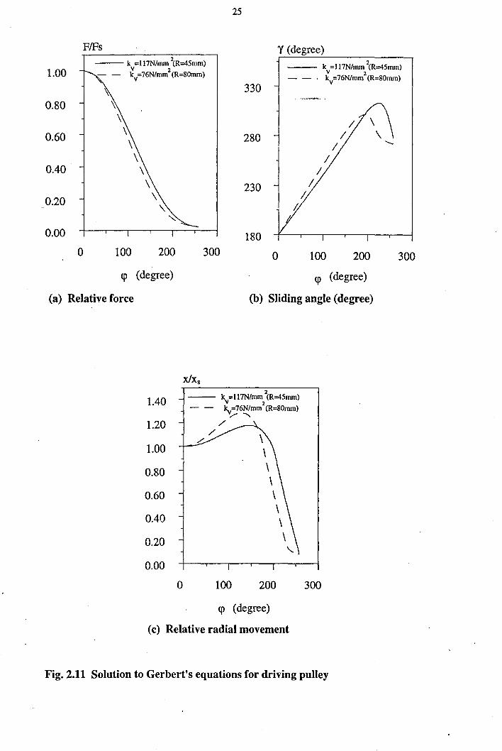
Figures 2.10a and 2.11a show the force variation F I F, against the active arc

length q>. Values of q> above 180 degrees are in the region which causes extensive

slip of the belt, (S, located at an imaginary point outside the arc of contact). It can be

seen from these figures that for any particular force ratio F I F, the driving pulley has

a smaller value of q> and therefore a higher torque capacity.

The sliding angle 'Y in figures 2.lOb and 2.11 b starts from 180 degrees in both

cases: this is the idle arc value. On the driven pulley 'Y increases (the belt leads the

pulley) until skidding occurs. On the driving pulley 'Y increase (the belt lags the

pulley).

The radial movement for driven and driving are shown in figures 2.1 Oc and 2.11 c.

On the driven pulley radial movement increases from its idle arc value x / Xs and the

belt moves into the groove. On the driving pulley the radial movement again is

slightly inwards, at the beginning. The amount of radial movement as compared with

the driven pulley is small.

FIFs 9 --k =117N/mm 2(R=45mm)

v 2 / 8

7

6

5

4

3

2

1

o o

- - k =76N/mm (R=80mm) v /

/-/-

b

100

/ /

/ /

200

/ I

I

<p (degree)

(a) Relative force

300

xix s

20

15

10

5

0

0

.&'

24

y (degree) 180

-- k =117N/mm 2(R=45mm) v 2

170 kv=76N/mm (R=80mm)

160

150

140

130

120

110

o 100 200

<p (degree)

(b) Sliding angle (degree)

k =1l7N/mm 2(R=45mm) v 2 kv=76N/mm (R=80mm)

I I

I /

/ /

/ /

/ /.

~

300

100 200 300

<p (degree)

(c) Relative radial rnovernnt

Fig. 2.10 Solution to Gerbert's equations for driven pulley

25

FlFs 'Y (degree)

1.00 -- k =1I7N/mm 2(R=45mm)

v 2 -- k =1I7N/mm 2(R=45mm) v 2 k

v=76N/mm (R=80mm) - - . k

v=76N/mm (R=80mm)

330 0.80

0.60

0040

0.20

0.00

o 100 200

<p (degree)

(a) Relative force

lAO

1.20

1.00

0.80

0.60

0040

0.20

0.00

o

280

230 I.

h

180 300 o

/ /

/

100

I I

/

200

<p (degree)


-- k =1l7N/mm 2(R=45mm) v 2

- - ky=76N/mm (R=80mm) /' """-

/ /

\ \ \ \ \ \ \ \

100 200

<p (degree)

300

(c) Relative radial movement

Fig. 2.11 Solution to Gerbert's equations for driving pulley

300

26

Table 2.1 Numerical results for Gerbert's equations (driven pulley)

(a)· driven pulley, kv = 117 N I mm2 (R=45mm)

active arc relative belt sliding relative

length tension angle radial

(degree) (force) (degree) movement

0.000 1 180 1.000

28.648 1.045 160.827 1.110

57.295 1.167 145.701 1.414

85.943 1.386 134.758 1.928

114.590 1.720 127.424 2.671

143.238 2.200 122.726 3.696

171.885 2:873 119.689 5.091

200.533 3.803 117.741 6.986

229.180 5.080 116.423 9.555

257.828 6.826 115.564 13.051

(b) driven pulley, kv =76N Imm 2 (R=80mm)




0.000 1 180 1.000

28.648 1.050 157.561 1.140

57.295 1.198 140.659 1.539

85.943 1.459 129.258 2.202

114.590 1.862 122.210 3.158

143.238 2.448 117.856 4.485

171.885 3.281 115.278 6.313

200.533 4.450 113.616 8.833

229.180 6.082 112.585 12.322

257.828 8.355 111.897 17.161

27

Table 2.2 Numerical results for Gerbert's equations (driving pulley)

(a) driving pulley, kv = 117 N I mm2 (R=45mm) , .. ---..




0.000 1 180 1.000

28.648 .962 197.668 1.013

57.295 .862 214.684 1.050

85.943 .715 231.987 1.102

114.590 .541 249.806 1.152

143.238 .366 268.427 1.178

171.885 .214 287.850 1.142

200.533. .105 306.299 0.973

229.180 .044 313.346 0.512

257.828 .021 277.537 0.085

(b) driving pulley, kv =76N Imm 2 (R=80mm)




0.000 1 180 1.000

28.648 .955 201.163 1.029

57.295 .837 221.331 1.104

85.943 .667 241.097 1.201

114.590 .475 260.692 1.275

143.238 .296 279.714 1.267

171.885 .158 296.387 1.080

200.533 .075 301.945 0.606

229.180 .038 278.683 0.158

257.828 .023 271.922 0.081

28

2.3.3.3 Non-Linear Slip

The fractional speed loss when an idle arc exists can be detennined by equation

(2.17), for equal radius pulleys. Non-linea{speed loss when the whole angle of wrap

becomes active was also developed by Gerhert. He imagined the actual belt paths to

be replaced by fictitious paths, with angles of wrap sufficiently greater than a. (the

actual wrap angle) to contain an idle point, to obtain expressions for speed loss in

.the non-linear range (see Ref. 1 and 3 ). In terms of fictitious forces E:dg and E:dn'

acting at S on the driving and driven pulleys, fractional speed loss is

(2.39)

The variation of FIE: with <P in the fictitious system may be obtained from the

theory of the last section, resulting in Figs. 2.10 and 2.11 for the driven and driving

pulleys respectively and sketched again in Fig. 2.12. In order that the fictitious and

actual systems match over the actual angle of wrap.

[~] =~. F q>=q>. F

s sdg on the driving pulley (2.40)

on the driven pulley (2.41)

These pairs of simultaneous equations determine unique values for <Po and E: in

the fictitious system. E:dg and E:d,. can be expressed in terms of F, and F,.

respectively to convert equation (2.39) to

F s=[ I

(FIE:),. Todg

F,. ][1 1] (FIF) ;+ k R2

s 'Pod,. V

(2.42)

29

Slip (s) can be seen to become non-linear in (F, - F,) as the values of C; )'1'0 . s

depart from 1.0. In practice in a drive consisting of two equal pulleys, the driving

.. pulley always has an idle arc, because torque is limited by slip on the driven pulley.

(£)'1' = 1.0, but (£)'1' can become>1.0. The equation for s (equation 2.42) can F odg F odn

s s

be normalised and non-dimensionalised [1] to give

__ s_c_= F, I F, [ 1

(F, + F,) (F, IF, + 1) (F IF, )CPOdg

1 c (F IF) ][1 + k R2 ]

s CPot«,dn v

(2.43)

F, IF, can further be related to the traction coefficient A.

A. = F, - Fr = F, IFr - 1 F, + Fr F, IF, + 1

(2.44)

In Fig. 2.13, s cI(F, + F,) is plotted against A. for the data in tables 2.1 and 2.2. The

ends of the linear slip ranges are shown by the arrows.

Gerbert [18] later developed a unified approach for flat, v- and v-ribbed belts slip,

which we will discuss at section 2.4.2

7

6

5

4

3

2

1

0

0 100 200 300 cp (degree)

Fig. 2.12 Theoretical relations between FIFs and cp for matching real and fictitious system

2.00

1.50

1.00

0.50

0.00

sclFt+Fr

k =117N1mnr (R=45mm) v 2

- - ky=76N/mm (R=80mm)

0.00 0.20 0.40 0.60 Coefficient of Traction(A,)

Fig. 2.13 Theoretical slip sd(Ft+Fr) as a function of traction coefficient

30

2.3.4 Torque Loss

Torque losses in a v-belt drive basically are the same as for a flat belt, and arise

from two main sources. ~or the case of a v-belt a major part of external losses is due

to sliding in the pulley groove at entry and exit regions.

Torque and power losses were studied earlier by Norman [5] and Gervas and

Pronin [24,25]. Gerbert in his v-belt theory [3], calculated the fractional power loss

due to sliding in the active arc excluding entry and exit regions. The much larger

portion of the torque loss is the no-load loss due to hysteresis and wedging at entry

and exit.

Gerbert in later papers [26,27] considered the shear deflection and a non- uniform

pressure distribution across a thick belt. He also allows the belt to have stiffness, and

recognised other sources of power loss. The results given by Gerbert [26] are in

graphical form. Cowbum [1] reduced these to the approximate form

J.L ~ 0.4 TLex = 7.1O-3 J.L R(F, + F,.)[I +0.35 LnlOs(s 1 R4k1)]

J.L~0.4 TLen =3.l0-3J.LR(F, + F,)[I+0.28 LnlOs(sl R4k1)]

(2.45)

where TL is contribution to torque loss at exit from the pulley and TL is a ~

contribution at entry. s, is the belt bending stiffness. For J.L>0.4, torque loss remains

constant with friction and equation (2.45) is valid with J.L = 0.4.

Losses due to hysteresis during bending and carcass compression are reported

experimentally [25]. The bending hysteresis is given by the empirical formula

TL" = 4.71 RO.6 (Nm) (2.46)

and for the compression loss

(2.47)

According to Cowburn [1], their contribution to the total no-load losses when

R=177.5 mm and (F, + F,) = 800 N is TL" 1 TL = 40% and TLc 1 TL = 11 % . When

R=62.5 mm for the same tension, T L" 1 TL = 46% and TLc 1 TL = 19% ..

31

2.4 V-ribbed Belt Drives

The v-ribbed belt was introduced in the 1950s. It is a cross between a flat and a

v-belt. This belt is essentially a flat belt with v-shaped ribs projecting from the bottom

of the belt whic~ guides the belt and make it more stable than a flat belt. In the

original concept, the v-ribs of the belt completely filled the grooves of the pulley. For

this reason, the v-ribbed belt did not have the wedging action of the v-belt and

consequently had to operate at higher belt tensions. Later versions of v-ribbed belts

have truncated ribs to more closely emulate the wedging effect of a v-belt.

V-ribbed belts have recently been applied in accessory drives by the automotive

industry and they have become the dominating belt, and have thereby attracted some

research attention.

Due to the shape of the v-ribbed belt (Fig. 2.14), it is not obvious if a v-ribbed

drive functions as a v-belt or a flat belt. The design and shape of a v-ribbed belt

affects its radial movement in the pulley grooves. When rib bottom I groove tip

contact occurs the wedge action decreases. The beginning of the contact depends on

belt tension, fit between rib and groove, wear and material properties [28,29].

Compared with the normal v-belt, there are very few fundamental studies on the

v-ribbed belt drives. The purpose of this work is to investigate theoretically and

experimentally the factors that influence the mechanical performance of v-ribbed belt

drives. Investigating the mechanical performance of v-ribbed belt drives requires a

clear idea to be developed on radial movement of the v-ribbed belt and its effect on

the other parameters of the mechanism. In the following v-ribbed belt literature

related to this thesis will be reviewed.

Top

Cord

Cushion

Rubber

W±0.5

o 2~ = 41+ 1.5 -----/

(a) Belt

Outside Diameter

Pitch Diameter

(b) Pulley

32

B

=1.5 H = 5.5 ± 0.6 ...,.-I- --+-----r--.L.......::.-

r = O.l5± 0.05

Diameter Over Balls

Fig. 2.14 Cross-section of a K-section v-ribbed belt and pulley (dimensions mm)

33

2.4.1 Torque Capacity

Hansson [30] made some analyses of the operating conditions of a v-ribbed belt

and discussed how the geometries of the belt and the mating pulleys affect the

pressure distribution between the belt and the pulley. He mentioned that normally the

pulley is stiff in comparison with the belt. This means that in the contact zone

between belt and pulley the belt is deformed into the geometry of the pulley.

However, the pressure distribution between belt and pulley differs according to the

wedge angle of the v-ribbed belt in relation to the wedge angle of the pulley. Hansson

concluded that there are two principal causes, apart from tolerances in

manufacturing, explaining why the wedge angles of the belt and pulley are unequal.

First, the wedge angle of the belt changes with the curvature of the belt and, second,

wear may change the wedge angle of the belt. Torque capacity of a v-ribbed belt is

highly dependent on the pressure distribution. A poor fit between rib and groove

implies large local compression of the rib and a decrease in torque capacity.

Later, influence o,f wear on torque capacity and slip was measured

experimentally' by Hansson [31]. These measurements were made on a new belt, a

belt that had run for 500 hours and for 1000 hours. The slip as a function of

transmitted torque is shown in Fig. 2.15. There seems to be a small difference

between the curves. He explained that the most plausible reason why the slip

decreases for the worn belt is that there is a difference in the surface between the

belts even though the belts were prepared to be as similar as possible. Also, from

visual inspection, he deduced the small decrease in slip was due to smoother surface

of used belt (see Ref. 31,32 for belt surface roughness). However, his results showed

that the worn v-ribbed belts, even if there is contact between the outer diameter of

the pulley and the bottom of the belt (rib bottom I groove tip), will keep their torque

capacity during the run. Thus a v-ribbed belt continues to function as a v-belt and not

as a flat belt [31].

34

Slip% 0.14 0 new

• 500h 0

0.12 -0 1000h

0.10 -

• 0

0.08 -

0.06 - [)

0.04 - ! 0

• 0

0

0.02 - " ij

0.00 I I I I I I I

0 1 2 3 4 5 6 7 8

Torque (Nm)

Fig. 2.15 The slip as a function of transmitted torque in a v-ribbed belt [31]

2.4.2 V-ribbed Belt Slip

Extensive measurements of slip and torque loss with a thick flat belt running on

small pulleys by Childs et al. [10,11] exhibited higher slip and torque loss than

expected from simple theory. Amijima [33] measured the traction capacity and shear

deflection of a piece of v-ribbed belt pressed against a groove plate.

The experiments showed reduction in traction capacity for high loads. Influence of

shear was mainly considered and developed theoretically for explanation of these

phenomena by Gerbert using Amijima's results, not only for flat belt but also for v

and v-ribbed belts slip. He developed a unified slip theory considering the following

four contributions [18].

• Creep (along the belt)

• Compliance (radially)

35

• Shear deflection (radial and axial variation)

• Flexural rigidity (seating and unseating)

He mentioned that shear deflection of the belt is a major factor to consider when

dealing with belt slip. Within the idle arc (adhesion arc) the frictional forces are partly

released. They are transferred from the belt-pulley contact through the rubber to the

cord layer, thereby causing shear deflection along the belt. The shear deflection varies

both radially (flat, v- and v-ribbed belts) and axially (v- and v-ribbed belts). Flat, v-

and v-ribbed belts have different cross sectional shape and different contact pattern

between pulley and belt, which requires separate treatments of the shear deflection

analysis of the different belt types. The radfal movement also contributes to the shear

[18]. Gerbert applied Finite Element Analysis [PEA] to get the variation of shear

deflection by transmission force.

The radial movement (rubber compliance) contribution to the speed loss for all

types of belts is given by

-1 F x=-·-

k R (2.48)

where k is spring stiffness constant. This· theory for radial movement does not

consider the effect of slidi~g angle "( and non-linear part of slip due to skidding (see

section 2.3.3.3).

Finally Gerbert mentioned that on v- and v-ribbed belts running on small pulleys

the belt is relatively thick compared to the pulley radius. Therefore classical creep

theory predicts slip which is substantially lower than the measured ones. He

concluded by taking into account all of the four contributions and good experimental

data (especially the material data) that the fit between theory and experiments is very

good for three practical tension levels (Figs. 2.16,2.17). For lower tension the

measured slip level was higher than the calculated one. The reason is probable poor

fit between the belt and pUlley.

36

Slip Quantity 12 x

+ 147N + 0 196N 0

10 - • x 294N x +

- • 392N • 8 0 x

+ • 6 - 0 x • + • x

0 • 4 - + x • •

0 x.

2 - , .x • x

[J • Classic

0 I I I

0.0 0.2 0.4 0.6 0.8

Traction

Fig. 2.16 Experimental slip quantity ( c . L\ro) vs coefficient of traction A. F,+F, 0)

for different total tension (F, + F,), (v-ribbed belt). Comparison with "classical"

flat belt theory [23]

12

10

8

6

4

2

o

Slip Quantity

0.0

- '.. 147N . . .. 196N - _. 294N -- 392N

0.2 0.4 0.6 0.8

Traction

Fig. 2.17 Theoretical slip quantity ( c . L\ro) vs coefficient of traction A. for F,+F, 0)

different total tension (F, + F,), (v-ribbed belt) [23]

37

2.4.3 Gerbert's V-ribbed belt Theory

In a later paper [34] Gerbert recognised the different radial movement of a v-··'or."

ribbed belt from flat belt and v-belt. He explained that flat and v-belts are to some

extent free ,to move on the pulley or in the groove respectively. The design and

constraint of a v-ribbed belt limits its motion in the pulley grooves. Due to the shape

of the belt (Fig. 2.14) ribs can not penetrate the pulley grooves individually. Maximal

penetration (due to the high load or rib wear) is limited by the outer radius of the

pulley. When rib bottom I groove tip interaction occurs the wedge action decreases.

The extent of the reduction in the wedge action depends on belt tension, fit between

rib ,and groove, wear and material properties.

Three different cases can be identified for mechanical performance of v-ribbed

belt.

(i) Without rib bottom I groove tip interaction (due to low load or less wear)

(ii) With rib bottom I groove tip interaction

(iii) Mixed contact

A simple theoretical model was developed by Gerbert [34] to calculate variation of

gross slip torque (maximum torque capacity) versus total tension (F, + F,.).

(i) Without rib bottom contact - For this case, Gerbert assumed that a v-ribbed

belt without rib bottom I groove tip contact acts as a v-belt and applied the classical

v-belt formula (equation 2.11). In this formula the effect of sliding angle is

neglected.

l.:::~ m:l'J:;:~:TY U~RARY

38

(ii) With rib bottom contact - Gerbert in this paper [34] attempted to model the

reduction in traction capacity for high loads that was reported by Amijima [33]. Two

alternatives (Fig. 2.18) were traced

• Case 1- All normal load per unit length P N is taken at the bottom of the rib.

• Case 2- Normal load per unit length PN is shared between the side and bottom of

the rib.

Fig. 2.18 Wedge load p and bottom load p. of the rib v F

Case 1- For the first case he assumed that the ribs are not able to penetrate further

when the pulley hits the bottom of the rib. Thus the side load is constant and all

additional load is taken up at the bottom of the rib.

Fig. (2.18) shows a v-ribbed belt with both sides loaded (wedge load per unit

length Pv and bottom load per unit length P F). Vertical equilibrium yields (for one

rib)

The traction force per unit length along the belt is

39

Thus we get the relative traction

T 2Jl (pv + PF) -= (2.49)

Suppose at the instant that rib bottom contact is made (PF =0) PN has the value PN L

and then Pv = constant= PVL

• Then

PN =2pv sin~ L L

(2.50)

If further loading causes no change to PV'

(2.51)

Therefore

...I.-=~. PNL (1-sin~ )+ PN sin~

PN sin~ PN (2.51)

Case 2· For the second case he assumed that all the compressed rubber of the belt

(all rubber between cord and pulley) is subjected to a kind of hydrostatic pressure.

This implies that all vertical loads increases to the same extent (we will discuss in

chapter 3 about this assumption). Suppose that for PN > PNL

' additional loads

develop in both the side and bottom of the rib in proportion to the additional overlap

between belt and pulley. Then

2( )_2PF Pv - PVL ---=----A

SIn .... (2.52)

giving

(2.53)

(2.54)

Eliminating PF gives the relative traction

40

(2.55)

Gerbert then compared these two cases with FEA results and mentioned that the

second case is fairly close to the FEA results.

Thus he applied this concept in the following. T and P N are loads per unit length

on a piece of belt pressed against a grooved plate. In a drive application, belt tension

F presses the belt against the pulley (radius R) by the radial load per unit length FIR

= PN ,(see Fig. 2.18). Thus equation (2.53) is replaced by

F -= PN +4PF R L

Traction T is equivalent of increasing belt tension by

dF=TRd~

~ is angular co-ordinate. Thus equation (2.54) gives

Eliminating P F yields

where

dF = J.l F(F + A)d~

J.l (1 + sin ~ ) J.l F= 2· A

SInt-'

A = 1- sin ~ ( R) l+sin~ PNL

(2.56)

(2.56a)

(2.57)

(2.58)

(2.58a)

(iii) Mixed contact· Suppose that rib bottom I groove tip contact occurs only over

an angle ~ F (Fig. 2.19). At the beginning of that angle belt tension is

(2.59)

41

and at the end F, = tight side tension. Thus integration of equation (2.58) gives the

solution

F,+A ( ) -..!.-- = exp J.L Fep F FL +A

(2.60)

over the angle where contact occurs. This is a slight modification of Euler's equation.

Pure wedge action when rib bottom I groove tip contact does not occur is

Tmax =~= J.L • A Y

PN sm ... (2.61)

Pure wedge action takes place over an angle ep y • Slack side tension F,. prevails

at the beginning of that angle and FL at the end. Then Euler's equation gives the

tension ratio

F .-..b.. = exp(J.L yep y ) Fr

(2.62)

as long as pure wedge action occurs.

Maximal tension ratio becomes F, IF,.. Instead of tension ratio we can deal with

the coefficient of traction

'" =F,-Fr

max F+F t r

(2.63)

The total wrap angle is

a=epy+epF (2.64)

Gerbert [34] then performed some experiments to measure variation of the maximum

coefficient of traction ("'max) versus total tension (F, + F,.) and calculated the variation

of (A'max) versus (F, + F,.) by putting a constant value for PNL

(equations 2.59 to

2.64) and varying ep y from 1800 (minimum F, + F,. and without rib bottom contact)

to 00 (maximum F, + F,. and with rib bottom contact at all arc of wrap). He adjusted

the coefficient of friction so the experimental results fits the calculations. The results

showed that "'max decreased by increasing (F, + F,.).

F t

p~O v

42

(a) Without rib bottom I groove tip contact

p ;::0 v

(b) With rib bottom I groove tip contact

q>p (rib bottom contact)

(starting of contact)

(c) Defining the angles of pure wedge action (without contact) and rih bottom contact

Fig. 2.19 Defining the mechanism of rib bottom I groove tip contact

43

2.4.4 ,V-ribbed Belt Torque Loss

V -ribbed belt literature review showed nothing related to this subject, neither

experimentally nor theoretically. Torque loss contribution to power loss __ will be

measured experimentally for v-ribbed belt drives in this work.

2.4.5 Development of V-ribbed Belt in This Thesis

Literature review revealed that v-ribbed belt drive mechanics have been studied by

some authors. Study on mechanical performance of v-ribbed belt requires to have a

clear idea on radial movement and its effect on the other parameters. Because of the

belief that radial movement is important, it was measured in this thesis. Later chapters

deal with the Non-Contact Laser Displacement Meter (NCLDM) used in this work

(to measure radial movement) and with the results. In the next chapter a new theory

for v-ribbed belt mechanics is developed. Special attention is made to radial

movement.

44

CHAPTER THREE

V-RIBBED BELT THEORY

3.1 Introduction

Wedge action and radial movement of v-ribbed belt are the fundamental

differences in action between an ordinary v-belt and v-ribbed belt. Due to the shape

of a v-ribbed belt, wedge action and radial movement depend on pressure variation

along the belt and wear.

Three different cases can be identified for mechanical performance of v-ribbed

belt.

(i) Without rib bottom I groove tip interaction (due to low load or less wear)

(ii) With rib bottom I groove tip interaction

(iii) Mixed contact

Gerbert [34] in his v-ribbed belt theory assumed that v-ribbed belt acts as a v-belt

in the first case. For the second case he assumed that some portion of belt tension

45

will be taken by the groove tip. Then he considered two possibilities, which we

discussed earlier (2.4.2).

• All additional normal load is taken up at the bottom of the rib

• Additional normal load is shared between the side and the bottom of the rib

Gerbert assumed the additional load after starting rib bottom I groove tip

interaction is shared to the same extent between rib side and rib bottom without any

explanation. At a private communication [35] he said this was because the results of

this assumption were fairly close to the FEA results. However we will show later

(section 3.4) that this is not always the case. Here we develop a new theory.

For a theory development some assumptions must be made. The initial

assumptions for v-belt theory (2.3.3) are still valid. Furthermore we assume that v-. ribbed belt is a combination of a flat belt with width of B F and belt force per unit

length P F' and a v-belt with mean width of By and belt force per unit length py

(Fig. 3.1). Let us further assume that the radial movement of the flat belt partxF ,and

the radial movement of the v-belt part Xy are equal. This has the effect that the top

of the cord surface 'deflects radially in a uniform way across the belt width. It is

shown later experimentally (section 5.2.1) that this is the case.

Fig. 3.1 Flat belt part and v-belt part of of v-ribbed belt load

46

This gives

(3.1)

and

(3.2)

where, FF = flat belt part tension and Fv =v-belt part tension.

3.2 Equilibrium Equations

We consider the equilibrium for v-ribbed belt as a combination of flat and v-belt

theory from sections (2.2,2:3). Fig. 3.2 and 3.3 show the forces acting on a part of a

v-ribbed belt in the groove of a pulley. PF and Pv are distributed forces which are

taken by the rib bottom and rib side.

F+dF

~~-\-__ p ds P dscos~ -----I'---~~\ F v KI __ ~--+--- Jl ~ ds sin~ s

pdssiq3 .---+--~ v I---\:~~--+---Jl Pv ds co$ s

Jl PF ds

Fig. 3.2 Forces acting on a v-ribbed belt element

R P ds F

P ds vz

47

(FIR)ds B

Fig. 3.3 Perpendicular forces acting on a v-ribbed belt cross-section

The equilibrium of the belt element ds along the belt gives

and perpendicular to the belt

put

then

ds= Rdq>

dF =2PvBl cos~ssiny ]+2~ PF Rdq>

F =2pv[sin~-~ cos~scosy ]+2 PF R

3.3 Radial Movement

-'~''''~".-

(3.3)

(3.5)

(3.6)

(3.7)

This section deals with theoretical analysis for the flat belt and v-belt parts of a v

ribbed belt radial movement.

48

3.3.1 Radial Movement of V-belt Part,xv

The contributions, XVI ,xv2and XV3 for v-belt part radial movement will be --,~.-.

discussed here one by one by analogy with the discussion of section 2.3.3.1 for v-

belts.

(i) Axial Component, XVI

The axial pressure PVz is distributed over the groove face. This force causes the

belt to reduce its thickness (Bv) and to sink into the groove. From the geometry

(Fig. 3.4) we have

Mv 1 X =-_._-

VI 2 tan P

The axial strain (Mv I Bv) resulting from PVz (Fig. 3.3) is

Mv=~ Bv· HvE z

From equations (3.8,3.9)

X - PvzBv

VI- . 2HvEz tanp

Where Hv is the v-ribbed part thickness. If we write

2pvz XVI =

kl

where kl is a type of spring constant, then

kl = 4 tan p EzHv

Bv

(3.8)

(3.9)

(3.10)

(3.11)

This equation is the same as XI for v-belt theory. In the case of a v-ribbed belt,

rubber is not combined with fibre, therefore it can be considered as a homogeneous -

material. Then, Ex = E z = E and

kl = 4tanpE·Hv Bv

(3.12)

49

H Max v

Fig. 3.4 Geometry of radial movement and axial strain

Furthermore there is a small difference concerning belt depth (Bv) when dealing

with a v-ribbed belt. A v-belt has a constant depth. But depth of a v-ribbed belt ( Bv )

increases with radial movement (Fig. 3.4), or

Bv = constant for v-belt

Bv = BVm + x for v-ribbed belt

where BVm is the minimum or no load depth. It will be shown (section 5.2.2) that for

a k-section standard v-ribbed belt we can neglect the effect of variable depth, if we

use mean depth value for Bv' Then

BVM +BVm Bv =----

2 (3.13)

Here BVM is the maximum depth (Fig. 3.4). Consider equations (2.22,2.24) from v-

belt theory

50

then we can write

where,

f (y)= . cos~ + J.1 sin ~s sm~-J.1 cos~s cosy

(ii) Radial Component, X V2

(3.14)

The distributed force FIR on the top compresses the belt. This makes the rubber a

little wider and thus prevents inward motion caused by the force F. The contribution

(similar to XVI)' can be written

ll. Bv 1 X =--.--

V2 2 tan~

The axial strain (Mv I Bv ) from the Poisson effect is

ll.B Fv -= ·v

B 2RBE

where V is Poisson's ratio. If we write

_ Fv xV2 ----

Rk2

then

(3.15)

(3.16)

(3.17)

(3.18)

where k2 is a kind of spring constant. Gerbert [3] in the case of v-belt, made a - . rough estimation for k2 , when thickness and width are about the same and the cord

is placed on the top of the belt. He estimated kl I k2 = 0.5 for this case. In the later

papers [27,36] for a similar belt this figure is near 1.0. For v-ribbed belt from

equations (3.12 and 3.18)

51

kJ _ Hv·v -----k2 Bv

Considering Fig. 2: 1 ~ and putting H v = 2.4mm, Bv = 1. 78mm and v = 0.5 it can be

estimated kJ I k2 = 0.67.

(iii) Longitudinal Component, XV3

.. The cord and rubber are stretched by the force F. The belt becomes narrower and

sinks into the groove. Its contribution to the radial movement is

(3.19)

where k3 is a spring constant depending on Poison's ratio v. If this is matched by

strain resulting from the radial movement X V3 [3]

k = 2ctan ~ 3 V B v

(3.20)

and

(3.21)

Cowbum [1] showed that the contribution of k3 on total radial movement is very

small. Therefore it can be neglected. Then

From these observations and putting XV3 = 0, the total radial movement for v-belt

part of v-ribbed belt is

Fv 1 xv=-·_-R kv(y)

(3.22)

where,

(3.23)

52

3.3.2 ,Radial Movement of Flat Belt Part,xF

Flat belt part of the v-ribbed belt is subjected to a radial load FF I R, when it is

pressed against the rib of the pulley with pitch radius R. The compression is

1 FF X =-.-

F k R F

where FF I R = 2PF and kF is radial spring stiffness.

The radial strain (Fig. 3.4) resulting from PF is

then

xF 2PF -=--HF BFE

2PF HF X =--.-FEB

F

From equations (3.25 and 3.26)

k _ BFE

F-HF

From equations (3.12 and 3.27)

k H·H _I =4tan~. y ~ kF By·BF

(3.24)

(3.25)

(3.26)

(3.27)

Considering the geometry of v-ribbed belt and putting HF == BF, roughly it can be

estimated kl I kF = 2. Substituting Xy and xF (from equations 3.22,3.24) into

equation 3.1 gives

FF =....!L kF ky(y)

Consider equation (3.2), then

F 1 X=-'---

R ky(y) +kF

At origin point S (see next section)

F 1 x =-.---

S R ky+kF

(3.28)

(3.29)

(3.30)

53

For the v-ribbed belt we can write

F 1 x=-·-

S R kVR .. __ (3.31)

where kVR is total radial spring stiffness for v-ribbed belt.

(3.31a)

Now the speed loss (slip) can be determined by

F, - F,. F, - F,. s= +--'-~

C kVRR2 (3.32)

Here the effect of shear deflection and seating lunseating arcs have not been

considered.

3.4 Basic Equations

In our model, which can be justified by experiment (section 5.2.1), we assume a v

ribbed belt is a flat belt and a v-belt with same amount of radial movement, i.e.

Xv =XF =x

If we recall equation (2.22) for v-belt

Fv = 2Pv(sin ~ - Jlcos ~s cosy) R

Then from equations (3.22, 3.25,3.26, 3.28)

2pv (sin ~ - Jl cos ~ s cosy) 2PF ~~~--~--~--~=---

kv(y) kF

or

Put PF in equations (3.6, 3.7)

dF =2Pv(Jl cos~ssiny)+2Jl pv(sin~-Jlcos~scosy).~ Rdcp kv(y)

(3.33)

(3.34)

(3.35)

(3.36)

54

~-" Dividing the equation (3.36) by (3.37) we have a new modification to Euler's.·

equation for v-ribbed belt.

1 dF (3.38)

F dcp

This equation is for the driving pulley. In the case of the driven pulley the equation

(3.6) becomes

dF = 2Pv[/lcos ~s sin 'Y]- 2/lPF Rdcp

Therefore we have

(3.39)

Equations (3.38 and 3.39) are for a v-ribbed belt with rib bottom I groove tip contact

over whole arc of wrap. In these equations if we put kF = 0, it will reduce to

equation (2.23) for v-belt and it is applicable to a v-ribbed belt without rib bottom

contact.

At the boundary between the idle and active arcs (point S) the sliding angle

'Y = 1800• If we assume this point as an origin the variables referred to this point will

Introduce non-dimensional values:

55

F· - = F belt tension F 0

s

Fv = F. v - belt part o~ v - ribbed belt tension F Vo 'J s

-; = FFo flat belt part of v - ribbed belt tension s

x - = Xo radial movement Xs

x ~ = xVo = Xo v - belt part of v - ribbed belt radial movement Xs

x -L = X Fo = Xo flat belt part of v - ribbed belt radial movement Xs

Equations (3.29,3.38) in non-dimensional form will be

Xo = F;,( kv +kF )

kv(y) + kF

where

dFo = Fh(y ) dq> 0

k g(y)±/J._F k

hey) = V(y)

1 kF +--kV(Y)

Jl cos ~ sin y g(y)= . s

sm ~- /J.cos ~ cosy s

(3.41)

(3.42)

(3.43)

Apply F = FF + Fv and put Xv = X F = x, then we have the following equations for

belt tensions of flat belt part and v-belt part of a v-ribbed belt.

(3.44)

k F. F V(l)

v= . kv(y) +kF

(3.45)

56

Dividing the equations (3.44,3.45) by Fs these equations in non-dimensional form are

kF FFo = F: . ----'---

kv(y) +kF (3.46)

(3.47)

Sliding condition equation for v-belt (2.36) is also valid for v-ribbed belt.

d(:) x 1-(:) --' tany= 1-(-)+ '

dq> Xs Co

In the case of v-ribbed belt F I Fs ,must be replaced by Fv I Fvs. Then

d(x) 1-(f.:-) -_O-tan y = 1- (x

o) + Vr

dq> Co (3.48)

From equation (3.45) and considering origin

(3.49)

3.4.1 V-ribbed Belt Equations Solution

Equations (3.41, 3.42, 3.46, 3.47 and 3.48) and tan ~ s = tan ~ cosy, form 6

equations for the variation of Fo , Fvo ' FFo' Xo ,y , and ~ s with q> • These

equations also were solved numerically by the help of Maple V (mathematical

standard library software), [Appendix AJ. It requires input of the physical and

geometrical properties co' kv' k F' J.1 and ~ .

Solutions for the driven pulley are shown in Figs. 3.5 and 3.6 and for driving in

Figs. 3.7 and 3.8. These are for two different sizes of pulleys, de=45mm

(kv =117Nlmm2) and de=80mm (kv =76Nlmm2

). V-belt results are also

represented for comparing with v-ribbed belt solutions. Numerical results are

presented in tables 3.1 and 3.2. The belt properties are taken from chapter five

(kv = 117 N I mm2 and 76N I mm2, kF = 20N I mm2 ~ = 20° and J.1 = 0.32).

57

Figs. 3.5a and 3.6a show the force variation F I F; against the active arc length <p

for driven pulley and Figs 3.7a and 3.8a for driving pulley. Values of <p above 180

degrees are in the region which causes extensive slip 'of the.-oolt. It can be seen from

these figures that for any particular force ratio F I F, the driving pulley has a smaller

value of <p and therefore a higher capacity, same as v-belt theory.

The sliding angle "( in Figs. 3.5b and 3.6b for driven pulley and 3.7b and 3.8b for

driving pulley starts from 180 degrees in both cases, this is the idle arc value. On the

driven pulley "( decreases (the belt leads the pulley) until skidding occurs. On the

driving pulley "( increases (the belt lags the pulley).

The radial movement for driven and driving are shown in Figs. 3.5c to 3.8c. On the

driven pulley radial movement increases from its idle arc value x I Xs and the belt

moves into the groove. On the driving pulley the radial movement again is slightly

inwards, at the beginning. The amount of radial movement as compared with the

driven pulley is small.

It can be seen that for three variables Fo ' Xo and "( the trends are almost same,

but v-ribbed belt has smaller value for radial movement as compared with v-belt,

specially for driving pulley.

In practice rib bottom I groove tip contact in a v-ribbed belt occurs over some

part of the wrap angle. Due to wear and running time of the belt and its fitting on the

pulley groove every particular belt has a unique value of radial movement x, related

to the start of contact. In this case for that part of wrap angle without contact, the v

belt theory can be applied. For the remaining part of wrap angle the v-ribbed belt

theory is applicable. However, this point is a turning point for v-ribbed belt drives.

Gerbert [34] attempted to develop a theoretical model for a mixed contact, and dealt

only with the maximum coefficient of traction (see section 2.4.3). But, theoretical

modelling for the belt tension ratio in the case of mixed contact, is still missing. In

this case the wrap angle is divided into two parts.

58

a=<PF+<PV

where <P v is the length of that part of wrap angle without rib bottom I groove tip

contact and <P F is with contact. Before the beginning of contact, we can write (from

equation 2.23 and 3.43)

1 dF g(y) for driven pulley

for driving pulley (3.50a)

where F;. is the belt tension and <P L is angular position at the beginning of the

contact. For driven pulley the variation of sliding angle y, decreases from 180

degrees and for driving pulley increases from 180 degrees. Therefor the right hand

side of the above equations are negative (driven pulley) or positive (driving pulley).

After contact the belt tension varies according to the equation (3.38, 3.39 and 3.43).

g(Y)-J1·~ kv(y) ---. = ---.".---";"':':"':""

F)FL-F, d<p)'PL-1800 1 +_k_F_ kV(YI

1 dF for driven pulley

1 dF for driving pulley (3.50b)

By the help of NCLDM the beginning of the rib bottom I groove tip contact around

the arc of wrap <PL' can be determined (see section 6.2). Then the tension ratio for a

v-ribbed with mixed contact can be decided from figures 2.10 and 2.11 (solutions to

v-belt equations for driven and driving pulleys respectively) and figures 3.5 to 3.8

(solutions to v-ribbed belt equations).

The total traction force per unit length along the belt acting on rubber between

cord and pulley is T = dF I Rd<p (equation 2.56a). From equation (3.36) we can write

59

T = 2/lpy[(cos ~s sin y)+ (sin ~ - /lcos~s cosy).~] ky(y)

(3.51)

The traction force per unit length at v-rib part of rubber is (from equation 2.21)

(3.52)

The traction force per unit length at flat part of rubber (see Fig. 3.1) is (from

equation 3.35)

TF = 2/lPF = 2J.Lpy(sin ~- /lcos ~s cosy).~ ky(y)

(3.53)

From equation (3.37) the total normal load per unit length PH' (vertical equilibrium)

is •

Normal load per unit length of v-belt part is

Normal load per unit length of flat belt part is

PFN = PF = 2py(sin~- /lcos~s cosy)(~) ky(y)

(3.54)

(3.55)

(3.56)

The main difference between v-belt and v-ribbed belt theory is appearing k F ill

the equations after rib bottom I groove tip interaction take place. This causes the belt

total traction T to be divided into two components TF and Ty, tractions of flat and v-

belt parts of a v-ribbed belt (Figs. 3.9 and 3.10), and total normal load to be divided

into two companents of flat and v-belt parts (Figs. 3.11 and 3.12). The variation of

TF I T and Ty I T and PHF I PH and PHY I PH across the active arc of contact <p

depends on the value of kF I ky and sliding angle y. From equation (3.43, 3.51, 3.52

and 3.53) we can write

Ty -g(y)

y:= /l.~+g(y) ky(y)

(3.57)

60

(3.58)

and from equations (3.54, 3.55 and 3.56)

PVN = kV(Y) (3.59)

PN kv(y) +kF

PFN = kF (3.60) PN kv(y) +kF

(Tv - TF ) causes an internal shear force between flat belt part and v-belt part of v-

ribbed belt at rubber between cord and pulley.

When the belt approaches the whole skidding condition (maximum traction), the

sliding angle y == 90° and g(y) = J.!/ sin ~. Then we can write

Tv 1 Y:)y=90 = k

_,,-F -.sin ~+1 kV(y=90)

kF .sin~ TF ) = kV(y=90)

y=90 k T F .sin~+1

kV(Y=90)

(3.61)

(3.62)

Put y = 90° into equations (2.23 for v-belt or v-ribbed belt without rib bottom

contact and 3.38 for v-ribbed belt with rib bottom contact)

where

1 dF -'--J.! F dcp - v

1 dF -'--J.! F dcp - F

1 J.!v = J.!'-.

sm~

1 kF -+-'---sin ~ kV(Y=90)

J.!F = J.!' k 1+ F

kV(Y=90)

Then from equations (3.61 and 3.62) we have

(3.63)

(3.64)

(3.65)

(3.66)

61

Tv Jlv -T )Y=90 = k

Jl. F +Jlv kV(Y=90)

(3.67)

kF Jl._'--TF ) = kV(y=90)

T y=90 k Jl. F +Jlv

kV(Y=90)

(3.68)

Equations (3.56 to 3.68) are related to maximum traction (skidding condition) at a

v-ribbed belt with rib bottom I groove tip contact at whole of arc of wrap angle. This

means that rib bottom contact will occur at PN = FL I R = 0 (see section 2.4.3 about L

Gerbert's theoretical model for v-ribbed belt). Put PNL = 0 in equations (2.54, 2.58a

and 2.61)

Tv Jlv -=--'-.!..-

T Jlv +Jl

TF = 1 T Jlv +Jl

1 Jlv = Jl.-.

slO~

JlF=Jl·

_1_+1 sin~

2.

(3.69)

(3.70)

(3.71)

(3.72)

Equations (3.69 to 3.72) can be compared with equations (3.65 to 3.68). It can be

seen that Gerbert's assumption about the increasing vertical load to the same extent 2PF k k [2(pv - Pv

L) = ~] leads to V(y=90) = kF· But V(y=90) and kF depend on fit between

SlOp

rib and groove, wear and material properties, therefore it not obvious if these are

equal. We will discuss more about the experimental results at chapters 5, 6 and 7.

PIPs 7

v-ribbed belt I

6 v-belt

5

4

3

2

1

o o 100 200

<p (degree)

(a) Relative force

14

12

10

8

6

4

2

o

h

o

I h

300

100

62

'Y (degree) 180

170

160

150

140

130

120

110

o

v-ribbed belt

v-belt ." .~. ;>- .-~ .• ~ -.-.--

100 200 300

<p (degree)


v-ribbed belt v-belt

200 300

<p (degree)


Fig. 3.5 Solution to v-ribbed belt theory for driven pulley (de=45mm)

9

8

7

6

5

4

3

2

1

0

FlFs

I v-ribbed belt I

-- v-belt I I

I /

/ /,

0

~

0 100 200

<p (degree)

(a) Relative force

20

15

10

5

o o

63

y (degree) 180

v-ribbed belt 170 v-belt

,- .. ~"J)~

160 ~

~

150 ~

~ 140 ~

~ 130 ~

0-120 :--...

110

100 300 0 100 200

<p (degree)


v-ribbed belt - - v- belt

100 200

<p (degree)

300


Fig. 3.6 Solution to v-ribbed belt theory for driven pulley (de=80mm)

300

64

FIFs y (degree) 400

v-ribbed belt v-ribbed belt 1.00 - - v-belt

0.80 300

0.60

0.40 200

0.20 '\

"- -0.00 100

0 100 200 300 0 100 200 300

<p (degree) <p (degree)

(a) Relative force (b) Sliding angle (degree)

xlxs 1.4

-- v-ribbed belt - - v-belt

1.2 '\.

\ 1.0 \

\ 0.8 \

\ 0.6 \

\ 0.4 \

\ 0.2

. 0.0

0 100 200 300

<p (degree)


Fig. 3.7 Solution to v-ribbed theory for driving pulley (de=45mm)

65

FlFs 320

'Y (degree)

v-ribbed belt -- v-ribbed belt 1.0 v-belt 300

- - v-belt '\ \'

0.8 \ 280 \

260 \ 0.6 \ 240

\ \ 220 0.4 \

~ 200

0.2 \ 180 '\.

.......

0.0 160

0 100 200 300 0 100 200 300

q> (degree) q> (degree)

(a) Relative force (b) Sliding angle (degree)

xlxs

-- v-ribbed belt - - v-belt 1.4

1.2

1.0

0.8

0.6

0.4

0.2

0.0

0 100 200 300

q> (degree)


Fig. 3.8 Solution to v-ribbed theory for driving pulley (de=80mm)

66

Ty/T, TF/T Ty/T, TF/T 1.0 Ty/T

1.0 Ty/T TF/T TF/T

0.8 -I 0.8 -I 1 1 I 1

0.6 - 1 0.6 - 1

0.4 - 1 0.4 - \ \ \ \ "-

- ......... _----0.2 ....... 0.2

'""'"------

0.0 I I 0.0 I I

0 100 200 300 0 100 200 300 <p (degree) <p (degree)

(a) kv = 117 N I mm2 (b) ky =76Nlmm2

Fig. 3.9 Variation of belt tractions of flat and v- belt parts of a v-ribbed belt against active arc for driven pulley

Ty/T,1F IT Ty/T,1F IT 1.0 Ty/T 1.0 Ty/T

TF/T TF/T

0.8 0.8

0.6 0.6

0.4 \ 0.4 \ \ \ \ \ ;-- -;--,

/ -0.2 "- ./ '- 0.2 --0.0 0.0

0 100 200 300 0 100 200 300 <p (degree) <p (degree)

(a) ky =117Nlm~2 (b) kv =76Nlmm2

Fig. 3.10 Variation of belt tractions of flat and v- belt parts of a v-ribbed belt against active arc for driving pulley

67

PV/PN' PFN Ip N pV/PN' P FN Ip 0.90 Fv lF 0.90

FIF - - FFIF v

0.80 0.80 FFIF

0.70 0.70

0.60 0.60

. 0.50 0.50

0040 0.40 ----0.30 0.30 -/" --- /" -- /"

0.20 - 0.20 --0.10 0.10

0 100 200 0 100 200

<p (degree) <p (degree)

2 (b) k v=76N/mm 2 (a) k =117N/mm v

Fig. 3.11 Variation of belt normal load of flat and v- belt parts of a v-ribbed belt against active arc for driven pulley

0.90

0.80

0.70

0.60

0.50

0040

0.30

0.20

0.10

!'VN/p N' P FN Ip

/ /"

o

/ /

/ /

/

100 200 <p -(degree)

2 (a) k v=117N/mm

-

0.90

0.80

0.70

0.60

0.50

0.40

0.30

0.20

0.10

o

/

--FIF v FIF

F

100 200

<p (degree)

(b) k =76N/mm 2 v

Fig. 3.12 Variation of belt normal load of flat and v- belt parts of a v-ribbed belt against active arc for driving pulley

68

3.4.2 Non-Linear slip

In the case of the v-ribbed belt the fractional speed loss when an idle arc exists can

be detennined by equation (3.32), for equal radius pulleys. Similar to v-belt theory,

non-linear speed loss when the whole angle of wrap becomes active can be

detennined by assuming fictitious paths with angles of wrap sufficient greater than a.

(actual wrap angle) to contain an idle point. Non-linear speed loss can be detennined

by the equation (2.43) from v-belt theory by replacing ky by kyR •

sc F,IF; [ 1 (F, IF; + 1) (F I F; )cp

odg (F,+F;)

In Fig. 3.13, sc/(F, + F,.) is plotted against A. for the data if. tables 3.1 and 3.2.

The ends of the linear slip ranges are shown by the arrows. The v-belt results are also

presented in these figures.

2.00 sc/(Ft+Fr)

1.50

1.00 .

0.50

0.00

v-ribbed belt v-belt

0.00 0.20 0.40 0.60

Coefficient of Traction (A.)

2 (a) k =117N/mm

v

2.00

1.50

. 1.00

0.50

0.00

sc/(Ft+Fr)

-- v-ribbed belt ___ v-belt

/ A

0.00 0.20 0.40 0.60 .

Coefficient of Traction (A.)

2 (b) kv =76N/mm

Fig.3.13 Theoretical slip sc I (F, + F;) as a function of traction coefficient

69

It can be seen that the slip value of v-ribbed belt is slightly lower than the v-belt,

but the difference is not significant. This is same as Hansson's experimental results for

v-ribbed belt wedge action (radial movement) and slip [31]. As discussed.:earlier

(2.3.1), his experimental results showed almost no difference between v-belt and v

ribbed belt torque capacity and slip, even for worn v-ribbed belt.

Experimental works and their results will be discussed later (chapter 6 and 7) and

it will be shown that it is not possible to predict the start of rib bottom I groove tip

contact theoretically due to miss-fitting and wear of any particular v-ribbed belt. This

point can be determined experimentally and then it is possible to apply v- or v-ribbed

belt theory to the drive for each part.

70

Table 3.1 Numerical results for v-ribbed belt equations (driven pulley)

(a) driven pulley, kv = 117 N I mm2

active relative sliding relative relative relative relative relative

arc belt angle radial v-belt flat belt v-beit flat belt

length tension (degree) move- part part part part

(degree) (force) ment normal normal traction traction

load load

0.000 1 180 1 0 1 .854 .145

28.648 1.068 158.191 1.141 .753 .247 .843 .156

57.295 1.217 143.180 1.465 .821 .179 .824 .175

85.943 1.454 132.638 1.959 841 .159 .803 .196

114.590 1.798 . 125.648 2.644 .847 .153 .785 .214

143.238 2.273 121.064 3.552 .849 .150 .771 .228

171.885 2.915 118.085 4.746 .850 .149 .762 .237

200.533 3.773 116.194 6.312 .850 .149 .755 .244

229.180 4.914 114.876 8.378 .850 .149 .751 .248

257.828 6.427 113.960 11.099 .850 .149 .747 .252

(b) drivenpulley,kv =76Nlmm2


arc belt angle radial v-belt flat belt v-belt flat belt


(degree) (force) ment normal normal tension tension

load load

0.000 1 180 1.000 0 1 .791 0.208

28.648 1.084 154.295 1.179 .694 .305 .773 0.226

57.295 1.258 138.081 1.565 .763 .237 .740 0.259

85.943 1.529 127.252 2.133 .781 .219 .709 0.290

114.590 1.915 120.377 2.897 .. 786 .214 .684 0.315

143.238 2.442 116.137 3.897 .787 .213 .667 0.332

171.885 3.151 113.444 5.202 .787 .213 .656 0.343 .

200.533 4.092 111.725 6.903 .786 .214 .648 0.351

229.180 5.339 110.579 9.146 .786 .214 .643· 0.356

257.828 6.987 109.777 12.088 .786 .214 .639 0.360

71

Table 3.2 Numerical results for v-ribbed belt equations (driving pulley)

(a) driving pulley, kv = 117 N I mm2




(degree) (force) ment normal normal tension tension

load load

0.000 1 180 1.000 0 1 .854 .145

28.648 .921 208.267 1.030 .791 .209 .836 .163

57.295 .780 229.925 1.085 .843 .156 .796 .203

85.943 .608 251.582 1.141 .849 .150 .726 .273

114.590 .436 274.157 1.158 .831 .168 .612 .387

143.238 .294 296.215 1.082 .790 .209 .462 .537

171.885 .195 306.815 0.824 .758 .241 .383 .616

200.533 .129 295.069 0.467 .793 .206 .471 .528

229.180 .087 279.943 0.253 .823 .176 .575 .424

257.828 .059 274.500 0.158 .831 .169 .609 .390

(b) driving pulley, kv = 76N I mm2




(degree) (force) . ment normal normal tension tension

load load

0.000 1 180 1.000 0 1 .791 .208

28.648 .900 217.263 1.072 .750 .. 249 .751 .248

57.295 .731 245.051 1.185 .787 .212 .662 .337

85.943 .545 271.177 1.243 .767 .232 .524 .475

114.590 .387 291.345 1.130 .724 .275 .391 .608

143.238 .271 293.580 0.811 .717 .282 .376 .623

171.885 .191 283.610 0.509 .743 .256 .444 .555

200.533 .135 276.792 0.331 .757 .242 .489 .510

229.180 .097 274.042 0.230 .762 .237 .506 . .493

257.828 .069 272.610 0.160 .764 .235 .514 .484

72

CHAPTER FOUR

BELT TESTING RIG

AND

INSTRUMENTATION

4.1 Introduction

In the following chapter the test rig and attached devices will be described.

Experiments were carried out on a dynamometer which was built to test belts. It was

used by Cowburn [1] for v-belt experimental investigations. New devices are

attached and used to make it more capable for v-ribbed belt tests.

It consisted of two trunnion mounted DC motors regeneratively coupled

(Fig.4.1). One was permanently fixed to a bed while the other was free to slide on

rails. This enabled a constant tension to be applied to the belt under test. The sliding

motor could also be clamped to provide a fixed centre drive arrangement.

The dynamometer was instrumented to measure the speed of both pulleys

separately. Torque exerted by the belt on each pulley could also be measured

separately.

73

Radial movement was measured by the help of a Non-Contact Laser Displacement

Meter (NCLDM) attached to the fixed motor. An intelligent multi-meter was used for

averaging the readings of torques.

4.2 Dynamometer

Fig. 4.1 shows the fixed motor A, and sliding motor B. Two identical 10 kW rated

D.C. motors (Mawdsley's Ltd. type 200N) were used, with their shafts facing. The

full range of belt length availa~le on the rig was 625< L < 1375 mm long, which

covers the general automotive range[37,38]. The motors were regeneratively coupled

and their roles as generator or motor could be reversed.

They were thyristor controlled (Mawdsley's type DSUA 1717a) and capable of

operating at speeds from 600 to 6000 RPM in their rotational direction. The motors

were fan cooled but could be driven for short periods without the fans.

The movable motor was mounted on linear bearings (RHP Roundway units Rw-8-

sand Rw-8-v) and set to run perpendicular to the fixed motor shaft. Tension forces

were applied to the belt by a dead weight and hanger system attached to the sliding

motor. The line of action of the force was in line with the pulleys to avoid rotational

forces on the sliding motor. A rigid frame supported the motors. This was set on 7

rubber machine mounts (Sunnex Ltd. Model 2) which were height adjustable by 53

rom, allowing the rig to be levelled.

A viscous dash pot (Kinetrol Ltd. Model KD-A300) was connected between the

motors, to damp linear vibration.

(a)

w

B

(b)

74

Trunnion Mounted Regeneratively Coupled, D.C. Motors

Dashpot

A

(Not to Scale)

Fig 4.1 Schematic of thebelt testing rig [1]

75

4.3 Instrumentation of Dynamometer

The dynamometer was instrumented to measure the values of radial movement,

speed and torque. The" following section is about the technical specifications of these

devices.

4.3.1 Non-Contact Laser Displacement Meter

Radial movement is recognised from larger axial force on the driving pulley than

that on driven (see 2.2.2). The fundamental difference in action between a flat belt,

v-belt and v-ribbed belt drives is their different radial movement performance. Thus it"

is important to analyse this phenomenon theoretically (see chapter 3) as well as to

measure it experimentally. Gerbert [3] measured radial movement of v-belt for two

sliding angles "( = 1800 and "( =900 by a dial gauge for static case. Cowbum [1]

carried out the measurement on v-belt by a dial gauge rotating with pulleys at low

rotation speed and with no torque transmission case. Hyunsoo Kim et al [39,40]

measured the radial movement of a metal v-belt CVT and a rubber v-belt CVT by

specially designed displacement sensors and strain gauges. This device was a contact

displacement meter.

Non-contact displacement devices were used by some authors [41,42,43,44] for

vibration and noise measurements. For the first time a Non-Contact Laser

Displacement Meter (NCLDM) has been used in this work for measurement of radial

movement of v-ribbed belt.

This equipment (Anritsu Corporation, type KL133B) which uses visible red laser

light as the light source, measures the . displacement of objects at high precision

without contact._1t can measures the dimensions of an object, including the height,

step difference, width and thickness. The dynamic response of mechanical elements,

also can be measured by this equipment.

76

The equipment consisted of a sensor head containing the optical system, a sensor

processing unit for processing the signal from the sensor head, and a display unit for

displaying the measured values (Fig. 4.2).

The sensor processing unit was mounted in the rear of the display unit. A three

meter signal cable was used to connect the sensor head and sensor processing unit

[45].

The repeatability of equipment was ±O.03% of the measuring range, and it had

16 steps of number of averaging. More detailed specifications are shown at

[Appendix Band C].

Display Unit

Sensor Processing Unit

Conection Cable

Power Cord

(Not to Scale)

Fig. 4.2 Schematic of the non-contact laser displacement meter

Fixing the device to the dynamometer by the ordinary stands was not possible ..

Therefore a special stand was designed and fitted to the dynamometer. The

configuration of this arrangement is shown in FigA.3. By the help of this stand the

radius of drive could be measured precisely at different angular positions.

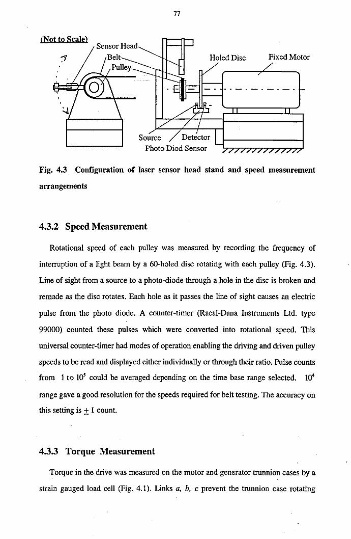
77

(Not to Scale)

Fixed Motor

Source Photo Diod Sensor

Fig. 4.3 Configuration of laser sensor head stand and speed measurement

arrangements

4.3.2 Speed Measurement

Rotational speed of each pulley was measured by recording the frequency of

interruption of a light beam by a 60-holed disc rotating with each pulley (Fig. 4.3).

Line of sight from a source to a photo-diode through a hole in the disc is broken and

remade as the disc rotates. Each hole as it passes the line of sight causes an electric

pulse from the photo diode. A counter-timer (Racal-Dana Instruments Ltd. type

99000) counted these pulses which were converted into rotational speed. This

universal counter-timer had modes of operation enabling the driving and driven pulley

speeds to be read and displayed either individually or through their ratio. Pulse counts

from 1 to lOS could be averaged depending on the time base range selected. 104

range gave a good resolution for the speeds required for belt testing. The accuracy on

this setting is ± 1 count.

4.3.3 Torque Measurement

Torque in the drive was measured on the motor and generator trunnion cases by a

strain gauged load cell (Fig. 4.1). Links a, h, c prevent the trunnion case rotating

78

under torque. Link c is the load cell. It is protected from shock loading and damped

by a rotational viscous dash pot. These transducers were capable of recording the

.,.,.maximum torque 25 Nm available from the motors. A transducer meter (Sangmo

Schlumberger type C56) was used to display the readings. This was fitted with a

digital L.E.D. indicator module, two transducer amplifiers and a summation module.

The digital display had a full scale reading of ± 1000. Either of amplifier's six range

settings from 0.25 to 100 could be set to read ± 1000 at full scale deflection of the

load cell. This gave the required accuracy. The summation module was able to read

the difference between the two channels, being useful for torque loss measurements.

Torsional vibrations in the motor trunnions were damped. Sm~ll roller bearings in

the connection rods were found to be necessary to avoid frictional interference

affecting the readings.

Digital display was given every third of a second and because of vibration in the

drive, accurate manual readings were difficult in all but the smoothest drives. To

alleviate this problem Cowbum [1] used a microprocessor, but in this work an

intelligent multi meter (Thuby-Thander Ltd. type 1905) was connected to the

transducer meter. This multi meter had an averaging mode, to average the readings.

This enabled the average of torque and torque loss, lowest reading and highest

reading that occurred while the program was being run to be stored in memory for

recall later .

4.4 Rig Calibration

There are some sources of apparent measurements in the rig. which must be

identified and separated from the actual values. In the following these sources will be

discussed.

79


An unload belt fits the pulley at a reference radius R, e.g. the pitch radius. When

the belt is loaded by the force F we get ~f'raoial movement x and the belt fits the

pulley at a radius R-x. The fit of a v-ribbed belt in the corresponding pulley is shown

in Fig. 4.4. The true pitch radius R of a v-ribbed belt drive is slightly larger than

effective radius (outside radius) Re. The surface of pulley shoulder (the actual outside

diameter) was used as a reference surface for radial movement measurements.

Position of the pitch zone

Fig. 4.4 Determination of pitch diameter

- -Jt,.- - --

Tb Hz. e

R R e

By the help of NCLDM (see section 6.2) the difference between the top of the

belt cord and pulley shoulder H T was measured at different runnIng conditions

around the pulley. These readings show very accurate values for the variation of the

radial movement around the pulley. The stand was attached to the fixed motor, and

the radial movement for driven and driving pulleys was measured by changing the

role of motors as a generator or motor. Two different points must be considered

regarding radial movement of the belt.

80

(i) The radial movement x, shows a linear and stable relationship with belt tension F

at high tensions, but at low tensions (F<150N) it is distinctly non-linear and unstable

(see"'-sectiCnis· 5.2.2 and 6.2). Therefore determination of an exact value for· pitch

radius R at no-load (F=O) is difficult. In this work, the main interest is to measure

change of radial movement. Instead of selecting the datum as the no-load (F=O) pitch

radius, at every total tension (F, + Fr ), the datum was chosen as the radial height HT

at angular position 90 degrees when there was zero torque transmission (T=O) and

no slip (s=O). This choice showed a very good stability and repeatability. Thus this

point was chosen as a reference point for the experimental measurements of the

variation of radial movement xe and

(ii) A small amount of wear occurred during each set of data collection, due to

experimental method and long running time of each set of the tests (see section 6.2)·

giving rise to an apparent radial movement xa. The apparent radial movement was

corrected by measuring the value of H T at the beginning and end of each set at

applied torque T=O. Then !J.xe can be calculated from

(4.1)

4.4.2 Slip Calibration

In this work both pulleys were of nominally equal size. Because of manufacturing

errors a small difference in their diameters was noted. This resulted in the pulleys

running at different speeds and giving rise to an apparent speed loss. The apparent

speed loss must be corrected for calculating the actual speed loss caused by slip of

the belt. This is achieved by multiplying the speed ratio of the driven to driving

pulleys, 0) dn 10) dg by the pulley radius ratio Rdn I Rdg • Slip in the drive. is then

calculated from

81

(4.2)

Pulley effective diameters (Fig. :4..4) were measur~9 with a micrometer and the results

are shown in table 4.1.

Table 4.1 Pulley diameter measurements

Nominal Pulley Effective Diameter Measured Pulley Effective Diameter

d=45 e (on fixed motor) dea = 45.16 (on fixed motor)

d=45 e (on sliding motor) dea =45.08 (on sliding motor)

d=80 e (on fixed motor) dea = 80.15 (on fixed motor)

d=80 e (on sliding motor) dea = 80.12 (on sliding motor)

To determine the values of pitch radius R, the difference between the top of the

belt cord and pulley shoulder HT was measured at no load (T=O) and no slip (s=O) .

condition for every total tension (F, + F,). As shown in figures 2.14 and 4.4, the

value of R for slip measurements for a standard K-section v-ribbed belt is determined

by

R = Rea +(HT -1.6)mm (4.3)

This method was only used for the ratio Rdn I Rdg • For other cases the pulley pitch

radius was taken R = Re + 1. 5mm.

4.4.3 Torque Calibration

In the rig the rotor and trunnion were locked together. Dead weights were hung at

a radius of 120 mm on the motor shaft. The weights were calculated to give a torque'

on the casing in steps of 2.67 Nm up to maximum 21.35 Nm. A transducer meter

(section 4.3.3) was used to record the torque. After a preliminary calibration to

establish linearity of response between torque and digital output (Fig. 4.5 and table

82

4.2), the amplifier gauge factors were adjusted to give a response of 427 digital units

for an applied torque of 21.35 Nm, with the amplifier at 2.5 range. The required

gauge factors were 4.98+0.02 and 5.25+0.03 for 'iKe: sliding" and fixed motor

respectively. The intelligent multi-meter (connected to amplifier) was adjusted to give

a response of 100+3 digital units for 1 Nm applied torque.

The intelligent multi-meter records the total torques 1'". and ~ acting on the

motor and generator casings respectively. The total torque on the casing has

components

• T, from the belt. This is transmitted to the casing via the shaft and magnetic flux

between'the shaft and casing.

• Tw' from wind resistance to rotation of the rotor.

• 1;, • from the shaft bearings.

• T, , from the trunnion bearings.

3000

2000

1000

o

Digital Units

o 10 20 Torque (N.m)

(a) Sliding motor

3000

2000

1000

o

30

Digital Units

o 10 20 Torque (N.m)

(b) Fixed motor

Fig. 4.5 Response between transducer and digital output

30 .

83

Table 4.2 Experimental results for linearity between digital units and applied torque

applied torque digital units digital units

(N.m) (sliding motor) (fixed motor): ..

2.67 267 266

5.34 536 535

8.01 800 801

10.67 1068 1067

13.35 1335 1336

16.02 1602 1601

18.69 1868 1869

21.35 2135 2136

Cowburn [1] showed that losses due to bearings are negligible. To determine the

torque due to windage without the cooling fans on, the motors were run un-coupled.

Torque was measured for speeds between 625 and 3000 RPM. Results for the fixed

and sliding motors rotating clockwise and anti-clockwise are shown in Fig. 4.6. The

data is presented in table 4.3. The wind~ge torque versus speed plot shows almost a

linear relationship up to 3000 RPM. Calibration equation for windage versus speed in

rpm, approximately is

Tw =0.01+30xlO-6 ro (Nm) (4.4)

The motors were mounted with shaft facing shaft, when they were coupled with a

belt their directions of rotation were opposite. The total torque loss is calculated by

(4.5)

For ro=2000RPM

TL = (Tm - T,)-0.14 (Nm) (4.6)

The accuracy of device was approximately +0.03 Nm. This gives a large uncertainty

in the results at low values of torque loss.

84

Windage Resistance (N.m) 0.10 __ sliding motor clock wise

0.05

0.00

-0.05

-0.10

and fixed motor anti-clock wise _ _ sliding motor anti-clock wise

and fixed motor clock wise

o 123 Speed (RPM/WOO)

F.g. 4.6 Windage resistance against speed

Table 4.3 Experimental results for windage calibration

speed sliding sliding fIxed

(RPM) motor clock motor anti- motor clock

wise clock wise wise

(Nm) (Nm) (Nm)

625 .01 -.01 -.01

1000 .02 -.02 -.02

1500 .03 -.03 -.03

"2000 .04 -.04 -.04

2500 .06 -.07 -.06

3000 .08 -.09 -.08

fIxed

motor anti-

clock wise

(Nm)

.01

.02

.03

.04

.05

.07·

......

85

4.4.4 Total Tension Calibration

Tension was applied to the belt by the dead weights hanging on a steel cable

attached to the sliding motor and running over 'a v-notched pulley fitted--with ball

bearings. The sliding motor was mounted on rolling bearings. A coefficient of friction

of 0.005 was quoted for these bearings, but during a static test this was found to be

near 0.01, requiring 50 N to produce steady motion.

The friction under dynamic conditions was determined from the full skid limit

torque. Thus; when the belt approaches full skidding, the traction coefficient,

A = (F, - Fr) I (F, + Fr) has a limiting value.

Euler's equation (equation 2.11) is valid for the v-belt and the v-ribbed belt

without rib bottom! groove tip contact (see chapter 3). The limiting traction'

coefficient is then given by

ellCX/sinp -1 A =--"..---

max ellcx/sinp + 1 (4.7)

For the values of Jl= 0.32, a = 7t and~ = 20° (see section 5.3.3), Amax = 0.899.

Therefore a dynamic means of measuring total tension (F, + ~) is

(F, +~) = T~ Rdg • max

(4.8)

Full skid slip tests are presented in chapter 6. The additional friction correction

load of 50 N was considered in these tests. The reduction of contact anglea, also,

must be considered.

86

CHAPTER FIVE

V-RIBBED BELT

MATERIAL PROPERTIES

5.1 Introduction

There are two basic types of v-ribbed belt construction. Both types use a single-

unit tensile section (one row of tensile cords) which extends across the entire width

of the belt. These two types differ in the method use to form the ribs on the bottom

side of the belt.

• Fully molded ribs as shown in Fig. 5.1. These ribs are often covered with a rubber

impregnated fabric to give better wear characteristics of the drive.

• Ribs formed by grinding (cutting) the rib profile in a cured slab as shown in Fig.

5.2.

There are a total of five individual cross sections available for use on v-ribbed type

drives. These are the H, J, K, L, and M cross section deSIgnations when working with -

conventional English or USA units. The cross section designations for SI metric units

remain the same except that a "P" is added before the cross section designation letter

(PH, PJ, PK, PL, and PM).

87

Table 5.1 and Fig. 5.3 give the sheave or pulley groove dimensions for v-ribbed

belts of these five cross sections. These sheave groove dimensions are standardised

. ,,:~.: .. J:?y The Rubber Manufacturers Association, The Mechanical Power Transmission and ... The Rubber Association of Canada in standard IP-26. The distinctive feature of each

cross section is the spacing between the ribs [29].

fabric facing

Fig. 5.1 Fully molded v-ribbed belt construction [29]

ground surface

(no fabric or covering)

usually fiber loaded stock

usually truncated ribs

Fig. 5.2 V-ribbed belt with ribs formed by grinding [29]

88

Table 5.1 Sheave or pulley groove dimensions for v-ribbed belts

Cross Section H J K L M

Minimum

. Recommended 0.50 0.80 1.50 3.00 7.00 Outside

Diameter

Groove 40 40 40 40 40

Angle±0.25°

0.063 0.092 0.140 0.185 0.370

S· g ±0.001 ±0.001 ±0.002 ±0.002 ±0.003

r,

+0.005 0.005 0.008 0.010 0.015 0.030

-0.000

2a 0.020 0.030 0.038 0.058 0.116

0.013 0.015 0.020 0.015 0.030

rb +0.000 +0.000 +0.000 +0.000 +0.000

-01005 -0.005 -0.005 -0.005 -.010

hg (Minimum) 0.041 0.071 0.122 0.183 0.377

dB 0.0469 0.0625 0.1093 0.1406 0.2612

0.080 0.125 0.125 0.375 0.500

Se +0.020 +0.030 +0.050 +0.075 +0.100

-01010 -0.015 -0.000 -0.000 -0.000

*Summation of the deviations from "Sg" for all grooves in anyone sheave shall not exceed

+0.010"

Source: Ref.[29]

89

Outside Diameter

Pitch Diameter

Fig. 5.3 Standard groove dimensions [29]

Diameter Over Balls

A v-ribbed pulley for the automotive industry is characterised by the number of

grooves, the profile and the diameter. It is designated by a series of numbers and

letters as follows:

• The first letter "P" indicates a pulley.

• The first set of numbers indicates the number of grooves.

• The second set of letters indicates the groove profile.

• The second set of numbers indicates the effective diameter (outside diameter), in

millimetres.

EXAMPLE

P 3 PK 80

Pulley T

Number of grooves

Groove profile

Effective diameter(mm)

90

A v-ribbed belt for the automotive industry is characterised by the number of belt

ribs, the profile (Fig. 2.14) and effective length. It is designated by a series of

numbers and letters as follows:

• The first set of numbers indicates the number of belt ribs.

• The letters indicate the belt profile.

• The second set of numbers indicates the effective length, in millimetres [46].

EXAMPLE

3 PK 1400

Number of belt ribs --.IT T Belt profile

Effective length (mm)

'All of the main experiments in this work were carded 'out with a v-ribbed belt of

type 3-PK-1400 (cut, manufactured by Pirelli, Italy). Two pairs of equal size of

pulleys P-3-PK-80 and P-3-PK-45 were run with the belt. Subsidiary tests on torque

and speed loss were also carried out with cut, molded and anti-wear v-ribbed belts of

type 3-PK-900 (manufactured by Dayco, Italy). Both the molded and anti-wear belts

differed from the cut belts in their mode of manufacture. They were molded, without

a cover, but were made from different materials.

In the Jollowing the required material properties for the theoretical part of the v

ribbed belt calculations will be investigated.

91

5.2 Radial Spring Constants

V-ribbed belt radial movement is dependent upon the forces acting on the belt. -~ _ .. .-

The amount of settle is then determined by the elastic properties of the belt and the

friction acting at the wedge interface.

At a preliminary test ( next section) the v-ribbed belt showed the same value of

radial movement for flat belt part and v-belt part. The mathematical model developed

for mechanical performance of v-ribbed belt (chapter 3), requires two spring

constants kv and k F. In this theory two different cases were discussed. Before rib

bottom I groove tip contact, the radial movement Xv is linearly related to the force F

acting in the immediate region by a constant 11 kv. In this case the v-ribbed acts as a

v-belt. When rib bottom I groove tip contact occurs, the radial movement is related

to the force by a constant kVR = kv + k F ,where k F is the radial spring constant of

flat belt part.

5.2.1 Preliminary Test

By the help of Non-Contact Laser Displacement Meter (NCLDM) the variation of

the difference between the top of the belt cord and pulley shoulder HT (Fig. 3.4)

across the belt width was measured, for different belts (new and used) and for two

cases, with rib bottom/groove tip contact and without rib bottom/groove tip contact.

It was tested for different transmitting torques (0-23 Nmm) at 13 steps [Appendix D].

It was found that the variation of HT =+O.005mm across the belt width (table

5.2), for all of tested conditions. This could be related to the much higher stiffness of

the cord compared with the rubber. Therefore we can assume v-ribbed belt is a

combination of a flat belt and a v-belt, where they have the same amount of radial

movement.

92

Then the theory developed (chapter 3) for mechanical performance of v-ribbed

belt drives and the required values for theory were determined by the following

arrangements.

Table 5.2 Tests for the variation of Hr across the belt width at angular position 90°

pulley sizes total tension applied torque readings d ,mm

e (Ft +Fc ), N (T),Nm HT±O·005(mm)

0 3.422 200

45 4 3.508

(new belt) 0 3.380 300

6 3.508

0 2.997 80 200

8 3.047

(used belt) 0 2.936 600

23 3.018

5.2.2 Tests for Determination of Radial Spring Constant "v A new v-ribbed belt was run on the two pairs of equal size of pulleys de =45mm

and de=80mm, at a speed of 625 RPM with different belt tensions. To alleviate the

effect of miss-fitting, dead weights were hung on the drive to a total of 2F=588 N

and reduced to 2F=98.5 N (unloading) in llsteps. The rig ran at no load (T=O) and

no slip (s=O) conditions. The sliding angle was 'Y = 1800 for this case. To avoid

different uncertainties arising from moving the sensor head of NCLDM, the sensor

head was fixed at the middle of the contact angle (angular position =90 degrees) and

the pulley was moved on its shaft to measure Hr. The maximum drive radius Rr

(Fig. 4.4) can be calculated from

(5.1)

93

The variation of RT versus the belt tension is shown in Figs. 5.4a and 5.4b for

actual effective diameter dea =45.160mm and dea =80.150mm, respectively. The data

is given at table 5.3. The following points must be considered:

(i) With respect to the K-section v-ribbed belt geometry (Fig. 2.14), rib bottom I

groove tip contact will not occur if B T >3.1mm. The results showed no rib bottom I

groove tip contact for the applied tensions. This means v-ribbed belt acts as a v-belt

and the only spring constant is ky •

k __ !iF y - R·!iRr

(5.2)

where

R:::RT -1.6mm (5.3)

(ii) As can be seen !i F I !i Rr is almost constant at high belt tensions (more than 150

N), but at low tensions the relationship becomes distinctly non-linear. This arises

from the belt not quite fitting the groove. In practice this occurs in a drive

transmitting high torque for the slack side at entry to the driven pulley. The

developed v-ribbed theory also is not applicable for entry to pulley and exit from

pulley regions.

(iii) The other reason for a non-linear relationship between Rr and F even at high

belt tensions is due to variable belt contact depth in the case of v-ribbed belt. A v-belt

has a constant contact depth, but the contact depth of a v-ribbed belt increases with

radial movement (Fig. 3.4), or

By = constant for v - belt

By =BYm +x

94

In the case of v-ribbed belt (equation 3.7) the maximum variation of kl' can be

calculated from

k _ 4tan~E Hv'· ,-

Bv (5.4)

where Hv is

(5.5)

(5.6)

In the practical case, HM - Hm == 0.2 (mm). Considering the geometry of K-section v

ribbed belt H M == 2.4. !1 k, I k, = ±O. 04. The effect of variable depth is negligible.

(iv) The variation of kv for dea =80.150mm is from 33.22N Imm 2 to 76.1 N Imm 2

and for dea =45.160mm is from 38.12N Imm 2 to 117.57N Imm 2• The upper values

are related to linear parts of the curves. For the pulleys of two sizes, difference in kv

may arise from the fit of the belt in its pulley groove. The change in the wedge angle

of a belt due to bending from its natural radius to the pulley radius has been

considered by some authors [1,18,30]. In this work for each pulley size the high

tension value of kv was chosen to represent belt radial stiffness in the theoretical

modelling, e.g. for de=45mm, kv =117 N Imm 2 and for de=80mm, kv =76N Imm 2•

95

Radius, RT (mm) Radius, RT (mm)

, 25.905 43.460

25.855

43.410

25.805

25.755 43.360 -+----,--.--.------.-,---\

o 100 200 300 o 100 200 300

Belt Tension, F (N) Belt Tension, F(N)

(a) <\ =45mm (b) de =80mm

Fig. 5.4 The variation of radius Rr against belt tension F, for a new v-ribbed

belt

Table 5.3 Tests for determination of kv

belt tension reading,Hr(mm) reading,Hr(mm) radius,Rr(mm) radius,Rr(mm) F(N) (d~a=45.160mm) (d~a =80. 150mm) (d~a=45.160mm) (d~a=80.150mm)

49.25 3.340 3.405 25.920 43.480 71.50 3.316 3.390 25.896 43.465 93.75 3.298 3.374 25.878 43.449 116.00 3.283 3.361 25.863 43.436 138.25 3.269 3.351 25.849 43.426 160.50 3.256 3.340 25.836 43.415 182.75 3.246 3.331 25.826 43.406 205.00 3.237 3.323 25.817 43.398 227.25 3.226 3.315 25.806 43.390 249.50 3.217 3.307 25.797 43.382 271.75 3.208 3.300 25.788 43.375 294.00 3.200 3.293 25.780 43.368

96

5.2.3 Tests for Determination of Radial Spring Constant k F

After rib bottom ! groove tip contact, the force F, has two components

. Fv and FF. For this case a used v-ribbed belt was run in the same conditions as a

new belt. The variation of Rr versus the belt tension is shown in Figs. 5.5a and 5.5b

for actual effective diameter dea=45.160mm and dea=80.150mm, respectively. The

data is given in table 5.4. The results showed for the applied tensions there is rib

bottom I groove tip contact at all steps of test (Hr<.3.1mm). This means that the v-

ribbed belt acts as a combined flat and v-belt and the spring constant is

(5.7)

Where

The variation of v-ribbed radial constant kVR for dea =80. 150mm is from

53.74N Imm 2 to 97.77N Imm 2 and for dea =45.160mm is from 37.32N Imm2 to

135.1 N Imm 2• A value of kVR =140N Imm 2 was recorded by Gerbert [28] for a 4-

PK-890 type v-ribbed belt. Considering the values for kv' the variation of kF for

dea =80.150mm is from 20.52N Imm2 to 21.76N Imm2 and for d~a=45.160mm is

from -0.8N Imm 2 to 17.53N Imm2.The upper values are related to linear parts of

the curves. In this work the value of kF=20N Imm 2 was chosen. According to our

model (sections 3.3.1 and 3.3.2), and putting I(Y =90) = 1.291 and A; I k2 = 0.67 ,

(equatio~ 3.23), we have kv=1.61 k1• From section 3.3.2 and putting A; I kF = 2, we

can get kv =3.22kF. But kF depends on HF (equation 3.27) and HF varies by

running time of the belt and wear.

97

Radius, Rr (mm) Radius, RT (mm) 43.070

25.590

25.540

43.020

25.490

25.440 42.970 o 100 200 300 o 100 200 300

Belt Tension, F (N) Belt Tension, F(N)

(a) <\, =45mm (b) <\ =80mm

Fig. 5.5 The variation of radius Rr against belt tension F, for a used v-ribbed

belt

Table 5.4 Tests for determination of kF

belt tension reading, Hr(mm) reading, Hr (mm) radius, Rr(mm) radius, Rr (mm) F(N) (dea =45.160mm) (dea =80.150mm) (dea =45.160mm) (dea =80.150mm)

49.25 3.005 2.990 25.585 43.065 71.50 2.980 2.970 25.560 43.045 93.75 2.963 2.961 25.543 43.036 116.00 2.947 2.953 25.527 43.028 138.25 2.935 2.945 25.515 43.020 160.50 2.922 2.938 25.502 43.013 182.75 2.915 2.932 25.495 43.007 205.00 2.906 2.925 ·25.486 43.000 227.25 2.900 2.918 25.480 42.993 249.50 2.893 2.911 25.473 42.986 271.75 2.886 2.905 25.466 42.980 294.00 2.879 2.899 25.459 42.974

98

5.3 Coefficient of Friction

The transmision capacity of a belt is considerably dominated by frictional

, characteristics of belt surface contacting with pulley [47]:-In the following some

relevant works will be reviewed. The results of an experimental work for

determination of coefficient of friction of v-ribbed belt will be shown at the end of

this section.

5.3.1 Introduction

A detailed account of the development of rubber friction theory and experimental

discovery is reviewed by Roberts [48] and Barquins [49]. A brief account of the

relevant works is given in the following.

Classical theory of friction states that the coefficient of friction is independent of

load, sliding speed and the apparent area of contact and it is material dependent and

its static value is higher than its sliding value. Experimentally it was discovered

[50,51] that the friction coefficient of rubber increased with speed and decreased with

load [1].

A new approach to the study of the tribological properties of rubber was opened

in 1971 when Johnson et al.[52] showed that the area of contact between a rigid

sphere and the flat, smooth surface of a rubber-like material is greater than that value

which can be deduced from the classical theory of elasticity, because of the

intervention of molecular attraction forces of the van der Waals type for elastomers.

Schallamach [53] also observed that, in certain circumstances, when a blunt rigid

asperity moves over a rubber surface, the true sliding friction does not occur. Indeed,

waves of detachment propagate across the interface from the leading edge to the

trailing edge of contact area, with a velocity greater than the imposed speed, and it is

these provides relative motion between the two surfaces. When the viscous

properties of rubbers are increased, the detachment wave phenomenon does not

99

occur, waves are replaced by ridges which remain engraved on the rubber surface and

can lead rapidly to hard wear. Barquins [49] explained that when a blunt, rigid

asperity is brought normally near a smooth surface of a highly elastic solid such as

rubber, as soon as the distance becomes smaller than a few tenths of a micrometer,

the two solids are subject to molecular attraction forces of the van der Waals type.

These forces, which are predominant for distances greater than 20A 0 , are the prime

cause of the adherence of solids. Indeed, stronger bonding forces are usually screened

off by impurities absorbed on the surface. When the contact occurs under an applied

load P, molecular attraction forces act into and around the contact area and are

added to the load so that the contact is maintained by apparent load ~ > P. The

difference ~ - P represents an adherence force depending on the load P, on the

contact geometry (shape and size) and on the mechanical and surface properties of

the elastic solid. According to Barquins [49] some authors [51,54,55,56] showed that

the frictional force of rubber is very sensitive to changes in the applied load, sliding

speed and surface geometry.

Although much experimental work has been done studying friction, theoretical

developments are not yet advanced to be able to predict friction coefficient for

rubbers [1,57]. Experimental measurements is therefore needed.

5.3.2 Coefficient of Friction for V-ribbed belts

Determination of coefficient or friction for v- and v-ribbed belts is more

complicated than flat belts due to their wedging action and laminate construction of

several materials.

Wada, N. and Uchiyama, Y. [58] carried out an experimental work on friction and

wear properties of short-fibre-reinforced chloroprence rubber composites. These'

composites have been used widely in hoses, v-belts, etc.[59,60]. The composites

were examined in three sliding directions, corresponding to the longitudinal,

100

transverse and noanal directions of the uniaxially oriented polyamid fibres under

various loads at various sliding speeds, using both metal gauze and abrasive paper.

They reported very high speed dependence of coefficient of-frlctien- for some

experimental cases.

According to Gerbert [3] several empirical foanulas are reported to estimate

coefficient of friction for v-belts [61,62,63]. These empirical and semi-empirical

foanulas generally are given for classical construction wrapped belts. It is unclear

how these can be applied to other belts with different constructions.

However, the above review gives an insight into the factors that might influence

rubber belt friction.

5.3.3 Measurement Methods

A value for the coefficient of friction is required in belt theories. Gerbert [3] and

Cowbum [1] detennined the coefficient of friction for v-belts experimentally, in a

testing rig at wholly slipping conditions. Then they followed Euler's equation

F. . Ilex. -' = exp(-.-) F,. sm~

Dalgamo et al. [64] for synchronous belt carried out a test basically in the same

way. In the case of v-ribbed belt Gerbert and Hansson [28] estimated the coefficient

of friction from the gross slip limit in their experiments. The value of coefficient of

friction was given as Il = 0.31.

Recently Dalgamo et al. [65] using a test rig (Fig. 5.6) measured ~e tight side.

tension of a v-ribbed belt F, with a load cell and hanging a dead weight (40N) on the

slack side, for four types of v-ribbed belts (moulded, anti-wear, new and used cut

belts, the same as in this project), at pulley speeds between 0-30RPM. The contact

101

angle between belt and pulley was 90° and the pulley effective diameter was 80mm.

The results of measurement showed the friction of moulded and anti-wear belts

. steadily increased with sliding speed:· For the used cut belt the friction was constant

over most of the speed range. The friction of the new cut belt decreased with sliding

speed in low speed range, and afterwards kept constant [65]. The results, also,

showed that the molded and anti-wear v-ribbed belts have the highest friction. The

used belt showed higher friction than the new belt.

A v-ribbed belt without rib bottom I groove tip contact acts as a v-belt (see

Chapter 3). At complete slip the sliding angle "( = 90°. Therefore it is reasonable to

apply Euler's formula to estimate the coefficient of friction for v-ribbed belt without

rib bottom I groove tip contact.

_ sin ~ In F, Jl-- -a F,.

(5.8)

In this work the same rig (Fig. 5.8) was used hanging 30 N dead weight to a half

used cut belt (without rib bottom/groove tip contact) running with sliding speed of 15

RPM. A typical drive will have a typical sliding speed greater than 10 mmlsec [1]

which gives the pulley speed of 15 RPM for the pulley diameter of 80mm. The

contact angle between belt and pulley was 90°. The measured value for F, under

these conditions was F,=130 N. Applying Euler's formula for

~ = 20°, a = rc/2 and F,. = 30N gives Jl = 0.32.

However this may not be the true value operating in a real drive, but it is very

near to it. Further work in this area is recommended.

'Ul'l'._ ....... ~ .•

102

load cell

w J.1 = s~~ In(f 11'; )

Fig. 5.6 Test rig for coefficient of friction measurements

5.4 Extension Modulus, c

In belt theories an extension modulus c is defined by

F c=- (5.9) .

E

Where F is belt force and E is longitudinal strain. The extension modulus is

assumed constant in these theories. Cowbum [1] experimentally measured the value

of c, for three types of un-cut AVlO v-belts (raw-edge, wrapped and cogged) and a

cut piece of these v-belts. He reported up to a 25% reduced c value for cut belts.

Also it is reported [1,6] that belts may have 5% variation in extensional modulus due

to repeated loading.

However, Moore [66] carried out some tensile tests which showed the variation

of the belt tensile stiffness with temperature for six different types of belts. V-ribbed

belt had lowest stiffness, because of the cord being polyester rather than glass fibre.

The tests were carried out with a 9.525 mm gauge length of a 3-PK v-ribbed belt

103

[67]. At the temperature of 80°C tensile stiffness of v-ribbed belt was 7.3 KNlmm

length. The value of c can be calculated by

c = 7.3 x 9.525 = 69.5KN

Moore [66] carried out the tests with the same type and same manufacturer's v-ribbed

belt which have been used in the present work. Because of slightly low temperature

at experimental investigations (section 6.2), due to long period of setting (normally 1

hour) and short running time (normally 20 minute), the value of c=80 KN was chosen

for the extensional modulus. Gerbert and Hansson [28] reported a value of 93KN for

a 4-PK-ll 00 v-ribbed belt. The value of non-dimensional extensional modulus

c c =-

o k R2 V

(5.10)

was calculated for two different pulley diameters de = 80mm and de= 45mm. The

pulley pitch radius R was chosen 1.5mm greater than effective radius [46].

104

CHAPTER SIX

EXPERIMENTAL INVESTIGATION OF

V-RIBBED BELT PERFORMANCE

6.1 Introduction

Due to the shape of the v-ribbed belt (Fig. 2.14), it is not obvious if a v-ribbed

drive functions as a v-belt or a flat belt. The design and shape of a v-ribbed belt

affects its radial movement in the pulley grooves. When rib bottom I groove tip

contact occurs the wedge action decreases. The beginning of the contact depends on

belt tension, fit between rib and groove, wear and material properties [28].

In the following chapter tests have been carried out with three conditions of belts:

with rib bottom I groove tip contact and without contact and mixed contact. The

variation of v-ribbed belt radius (radial movement) at working conditions, slip (speed

loss) and torque loss on a two pulley rig are experimentally determined. The rig is as

described in chapter four.

Particular attention is paid to the radial movement and its dependence on other

factors. For the first time a Non-Contact Laser Displacement Meter (NCLDM) has',

been used for measuring radial movement of the v-ribbed belt in this work. By the

105

help of this device the variation of radial movement could be measured at the actual

working conditions and with very high precision.

6.2 Experimental Method

The beginning of the rib bottom I groove tip contact around the pulley depends on

belt tension, fit between rib and groove, material properties and wear. Thus any

particular belt has a unique value of radial movement x, related to the start of rib

bottom I groove tip contact, and it is not possible theoretically to predict this value.

But for all standard v-ribbed belts, considering their geometry (Fig. 2.14), a reference

point could be chosen for HT (Fig. 4.4), which shows the start of contact. For a PK

section v-ribbed belt we can write

H Tconlact = 3.1 (mm)

Rrcontact = Rea + H Tcontact

By the help of NCLDM the values of HT were determined for all of the tested v

ribbed belts. Thus it is possible to determine starting point of rib bottom I groove tip

contact.

The three type of contact: with rib bottom Igroove tip contact, without rib bottom

contact and mixed contact were obtained with new and used cut belts all of which

had the same material properties. In the following, tests described as "new v-ribbed

belt" refer to most tests in which the new v-ribbed belts were used : H T values

greater than 3.1mm indicated no-rib bottom I groove tip contact. In few cases, at

high tension (F, +F,=600 N) on a small radius pulley (de =45mm), the new bel(

gave mixed contact: this will be referred to as the "extreme condition" test. Other

tests were carried out on a cut belt that had been used long enough to create rib

106

bottom I groove tip contact in all conditions. These tests will be described as "used v-

ribbed belt" tests.

New v-ribbed belt = Test without rib bottom I groove tip contal:t

Used v-ribbed belt = Test with rib bottom I groove tip contact

Extreme conditions test = Test with mixed contact

Eight sets of experiments were carried out for each driven and driving pulley.

Two sizes of standard pulleys were used for mecha."1ical testing. These were paired

with nominal effective diameters, de =45 mm and de =80 mm (nominal angle of wrap

on each pulley is 180°). The minimum recommended effective diameter, de , for PK

pulleys is 45 mm. The tests were carried out at the speed of 0) =2000 RPM, which

was the smoothest running speed for the drive.

Table 6.1 lists the experimental tension and torque conditions. At each set of

experimental work, torque applied to the drive at three, four or five stages from 0 to

maximum (skidding condition).

Also some subsidiary tests were carried out with smaller intervals of applied

torque T, and five different v-ribbed belts, new, half-used, used (cut), new molded

and new anti-wear. During these tests slip and torque loss were determined

experimentally at two different speeds of ro=1000RPM and ro=2000RPM to better

compare variation of slip and torque loss between different belts at different speeds.

The variation of drive radius around the pulley was measured at 11 steps of

angular position,ap= 0, 10, 20, 30, 60, 90, 120, 150, 160, 170, 180 degrees. At entry

to the pulley and exit from the pulley regions, up to angular position of 30°, the·

intervals were chosen 10°. At the other positions the measurements were carried out

at 30° intervals.

107

Table 6.1 Range of variables in mechanical tests

Variables pulley sizes total.tension applied torque figure de,mm (Ft +Fr ), N (T),Nm numbers

200 0,2.5,4 6.1a,6.2a 45 300 0,2.5,5,6 6.3a 6.4a

driven pulley 600* 0,5, to, 13 6.9a

80 200 0,5,8 6.5a 6.6a 600 0, 5, to, 15,23 6.7a 6.8a 200 0,2.5,4 6.tb 6.2b

45 300 0,2.5,5,6 6.3b,6.4b driving pulley 600* 0,5, to, 13 6.9b

80 200 0,5,8 6.5b,6.6b 600 0,5, to, 15,23 6.7b,6.8b

* Extreme conditions test

The extreme conditions test was carried out on a pair of pulley sizes of

de = 45 mm for driven and driving pulleys. In this case, the variation of drive radius

was measured at 19 steps from 0 to 195 degrees, to consider entry to the pulley and

exit from the pulley regions, for maximum tight side belt tension and radial

movement.

To avoid different uncertainties, the sensor head of NCLDM was fixed at each

angular position, then the reference surface (pulley shoulder) and measuring surface

(top surface of the belt) was brought under the laser beam by moving the pulley on its

shaft. At each angular position the following steps carried out one by one;

1. Fixing the sensor head at the measuring angular position

2. Putting the reference surface under the laser beani

3. Hanging the required dead weight

4. Running the rig at no torque, T=O

108

5. Setting the laser meter to zero

6. Switching off the rig and removing the dead weight

7. Putting the measuring surface under the laser beam

8. Hanging the dead weight and running the rig

9. Applying the required torque and reading the meter

This method took a long time for each set, but it was completely convenient that

the collected data was accurate [Appendix C]. The readings showed the value of HT

(Fig. 4.4) for each running condition.

NCLDM was attached to the fIxed motor and the measurements for driven and

driving pulleys were carried out by changing the role of motors as a motor or

generator.

As discussed earlier (section 4.4.1) at low belt tensions the actual radial

movement x, was very unstable, therefore determination of exact value for pitch

radius (origin for x) experimentally, is diffIcult. At no torque (T=O) and no slip (s=O)

conditions for every value of total tension the readings showed a very good stability

and repeatability, especially at angular position (J.p = 90°. Thus this point was chosen

as a reference point for the experimental measurements of the variation of radial

movement (xe ).

It is possible to reconcile the theoretical results to this reference point.

Due to long running time of belts at each set of experiment (see section 6.2) a

small value of wear occurred during the test. These values were measured and

recorded (table 6.2) for each set by measuring HT at the beginning and end of each

set.

109

Speed ratio and torque loss were measured during the tests, usually choosing the

runs when radial movement measurements were taken at angular position

100 and 1700, Le. near the first and last test of run.

Table 6.2 The amount of wear during each set of tests (Jl m)

Fig. Fig. Fig. Fig. Fig. Fig. Fig. Fig. Fig.

6.1 6.2 6.3 6.4 6.5 6.6 6.7 6.8 6.9

a b a b a b a b a b a b a ·b a b a b

12 18 17 5 12 18 17 5 4 5 3 6 8 5 6 6 36 40

6.3 Fundamental Experiments

In the following section the radial movement, speed loss and torque loss occurring

on a two pulley rig are experimentally determined.


The variation of drive radius Rr = Rea + Rp versus the different angular position

is the subject of Figs. 6.1 (a and b) to 6.8 (a and b) for driven and driving pulleys

respectively. The variation of experimental radial movement xe is represented at the

right side of each figure. In each figure there are three, four or five graphs relating to

the values of applied torques. These figures, have been constructed from the data;

given in tables 6.3 to 6.6 and the experimental points have been omitted from figures

6.1 to 6.9 for clarity but can be deduced from the tables. The results for different

values of applied torque are compared.

110

In all of the figures the starting point for rib bottom I groove tip contact is

represented by a horizontal line. It can be seen that rib bottom contact does not occur

at any angular position for new belts. In the case of used belts, rib bottom contact

takes place at most tests, only for some few set of tests (Figs. 6.2 and 6.4) over some

part of angular position (towards slack side) at maximum transmitting torque the belt

comes out of rib bottom contact.

Considering the relationship between Rr and radial movement x, (!l. Rr = -!l. x) it

can be seen that for a driven pulley in the initial stages of entry to the pulley, radial

movement increases slightly and a more rapid increase occurs at exit region. In the

case of the driving pulley radial movement decreases slightly with increasing angular

position for the applied torque values less than the skidding condition (increasing

positive x, means movement towards the pulley centre).

For both pulleys (driven and driving) radial movement increases with increasing

values of applied torque.

The trend of variation of radial movement for the new belt (without rib bottom I

groove tip contact) is almost the same as for used belt (with rib bottom \ groove tip

contact), but it will be discussed in the next chapter that the value of radial movement

for used belt is less than new belt at all of the tested cases.

The bending stiffness of the belt reduces the arc of contact. The amount of

reduction of contact angle can be estimated from these figures for each set of tests. It

can be seen from figures 6.7, 6.8 6.9 that, due to low bending stiffness value of v

ribbed belt and high belt tension, at tight side for both driven and driving pulleys there

is not any reduction of contact angle. At relaxed side the reduction of contact angle

increases with increasing the value of applied torque.

Figs. 6.9 (a and b) show the result of an extreme condition test for driven and'

driving pulleys (data is given in table 6.7). The test were carried out with the smallest

recommended size of pulley (de = 45mm ) for PK section v-ribbed belts with total belt

111

tension (F, + F,.) = 600 N. The test covered 15° beyond the arc of contact (exit

region). The results for driven pulley show more rapid increase of radial movement,

and even after the geometric arc of contact. For the driving pulley there is a rapid

decrease of radial movement at the middle of the arc of contact and an increase

afterward.

Due to high value of total belt tension, (F, + F,.) = 600 N, mixed rib bottom I

groove tip contact takes place almost at all transmitting torques.

The amount of wear during this set is very much higher than the earlier sets and it

can be seen from the slope of the zero torque (Torque=O) radial movement. For

driven pulley 1:1 HT)T=O :::36J.l mm and for driving /). HT)T=O =40J.l m.

During the extreme condition tests the ribs of the two new v-ribbed belts

collapsed. This can be attributed to the internal shear force (at the rubber) between

flat belt part and v-belt part of v-ribbed belt. In section 7.6 we will discuss more

about this phenomena.

26.4

26.2

26.0

25.8

25.6

26.4

26.2

26.0

\ \

\ '-\ - . -

112

-- Torque=O.O Nm __ - Torque=2.5 Nm

"~ - • - Torque=4 Nm

. -. -. , -'-. "--'"---------- --------. -------_\

" \

-0.2

0.0

0.2

-+--,---,----r--.---,----'T.,.....--~-_t_ 0.4

o 45 90 135 180 Angular Position (degree)

(a) Driven pulley

R (mm) x e(mm) ---rL----------------___,...-=..-~ -0.4

-- Torque=O.O Nm - - . Torque=2.5 Nm - . - Torque=4Nm

I I I . I

.' I /'-'-.-.-.~ I

/

---" ---.::::. ... _------."". ,.,'" -.

-0.2

0.0

0.2 25.8 .

25.6 -+--~-~----,;--.,---~--.,.----.----I-- 0.4

o 45 90 135 180

Angular position (degree)

(b) Driving pulley

Fig. 6.1 Variation of drive radius and radial movement against angular position for a new v-ribbed belt (without rib bottom contact) (F, + F,=200 N,' d,=45 nun)

26.2

26.0

25.8

25.6

25.4

26.2

26.0

25.8

25.6

25.4

113

\

\

Xc (mm)

Torque=O.O Nm Torque=2.5 Nm Torque=4Nm

-0.4

\

\ -0.2

-_ .... ~_ .............. ::-:::-:::-:: =-=:::-: or _, ~ .............. _

.......... _------- --., ------~, 0.0

45

(a) Driven pulley

90 135 180 Angular Position (degree)

X (mm)

Torque=O.O Nm Torque=2.5 Nm

0.2

Torque=4 Nm 4 -0.

I ,

I I I -------' ----- / . .. ............................... -/- ............................ :,;- .... ..

\. -----:....--------~ -- _ ... \.--.--


(b) Driving pulley

-0.2

0.0

0.2

Fig. 6.2 Variation of drive radius and radial movement against angular position' , for a used v-ribbed belt (with rib boitom contact) (F, + F,=200 N, df!=45 mm)

26.5

26.3

26.1

25.9

25.7

26.5

26.3

26.1

25.9

·25.7

o

114

, \

x (mm)

Torque=O.O Nm Torque=2.5 Nm

-_,~ ..... ~,TQ.rque=5 Nm - - -Torque=6 Nm

" \ .. - .. - ---\. .. _---. \ .......... --.-.--.-.. .--- ....... -----. -.. '--------- ---.--, -- - --:- - - - - -~, "

45 90 135 180 Angular Position (degree)

(a) Driven pulley

o

(mm)

Torque=O.O Nm' Torque=2.5 Nm Torque=5Nm Torque=6Nm

-' -- . --.• c:::=.-':---

..... _ - - - - --:- L-: :::: =--• _ • __ :---: : .=-r _. -

... -- ....

45 90 135 Angular Position (degree)

x (mm)

: I I . . /

I

180

(b) Driving pulley

-0.4

-0.2

0.0

0.2

-0.4

-0.2

0.0

0.2

Fig. 6.3 Variation of drive radius and radial movement against ~gular position for a new v-ribbed belt (without rib bottom contact) (F, + F;=300 N, de=45 nun)

26.2

26.0 ..

25.8

25.6

25.4

25.2

26.2

26.0

25.8

25.6

25.4

25.2

115

R (mm) Xe (mm)

o

Torque=O.O Nm - - - Torque=2.5 Nm - . - Torque=5 Nm

\ . - .. - Torque=6 Nm

\ \ \ \, '

\ \ . \' \ .. _ .. _ .. _ .. - ..

. ,.\.:.::...:::....:::....:.::..:.::..: -.. -. ~ "" -~-.-.- ': .. : .- - - .. -- - - ----- ~---: = ~--= =. - .. , --


(a) Driven pulley

Torque=O.O Nm - - - Torque=O.O Nm

x (mm)

-0.4

-0.2

0.0

0.2

- • - Torque=O.O Nm -0.4 - .. - Torque=O.O Nm . I

I I I : / I -0.2

_ .. - / I - .. - . - .... - - .. - - ..... ,~:.-..... - : : - /.. .. ·,r -

. .,.,,- ------ ",-

____ - - - - -or - - -_"""""'='" ~ 0.0 : :--= :-: :.---: : -=-- - - - - -

0.2


(b) Driving pulley

Fig. 6.4 Variation of drive radius and radial movement against angular position for a used v-ribbed belt (with rib bottom contact) (F, + F,=300 N. d.=45 mm)

43.9

43.7

43.5

43.3

43.1

43.9

43.7

43.5

43.3

43.1

116

R (mm)

Torque=O.O Nm Torque=5Nm

- . - . To~ue=8 Nm

---------- .. -- - - - - - - - .: .. :-:-= == =---- .. - = ......... --=.

o 45 90 135 Angular Position (degree)

(a) Driven pulley

R (mm)

-- Torque=O.O Nm - - - Torque=5 Nm - . - Torque=8 Nm

- ... ---... .. ...- .. '" ------

180

x (mm)

/

.' I I I . I

.' I / I

/ ----------

o 45 90 Angular Position (degree)

(b) Driving pulley

135 180

-0.4

-0.2

0.0

0.2

-0.4

-0.2

0.0

0.2

Fig. 6.5 -Variation of drive radius and radial movement against angular position for a new v-ribbed belt (without rib bottom contact) (F, + F,=200 N; d

lt=80 mm) .

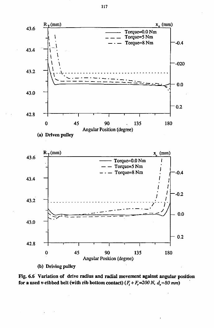
43.6

43.4

43.2

43.0

42.S

43.6

43.4

43.2

43.0

42.S

R,.(mm)

-\ \ I

\ " \ - \ I

\ \ - I

117

x~ (mm)

Torque=O.O Nm Torque=5Nm Torque=SNm --0.4

\ \ ~-~

-I~\ . :\'.' ................................. . " '----------------

- - - - - - - - - - - - - .:...-=-. -. - ...... 1-- 00 ~. .

-

-~0.2

I I I

0 45 90 135 ISO Angular Position (degree)

(a) Driven pulley

x (mm)

-- Torque=O.O Nm

I . -0.4 - - Torque=5 Nm

- . - Torque=S Nm I I I I

-0.2 I I . I .................................. /' .. } .

------------- . .. -- . - - -' 0.0 '":"r - - - - - - - - - - -

0.2

o 45 90 135 ISO Angular Position (degree)

(b) Driving pulley

Fig. 6.6 Variation of drive radius and radial movement against angular position for a used v-ribbed belt (with rib bottom contact) (F, +F,=200 N, de=80 mm) .

43.9

43.7

43.5

43.3

43.1

43.9

43.7

43.5

43.3

43.1

R

-. -.

- .

118

(mm)

. . .

Xe (mm) Torque=O.O Nm Torque=5Nm Torque=10 Nm Torque=15 Nm Torque=23 Nm

--0.4

--0.2 _.\ . I~: ....................... .

- ~\'-":-"'::". - .. - .. - .. - . : ............. . \" . ---- -- . - . - . - . -- .. - ... ~ -- - - - -- -..=- - - - .--==--.~. - 0.0

-

-

o I

45

I

90

I

135

.~

~

r- 0.2

180 Angular Position (degree)

(a) Driven pulley

-

--

-

-- ..

_ .... ~ ,r'1; "'-- - .='. -

-

x (mm) e

-- Torque=O.O Nm Torque=5Nm Torque=10 Nm Torque=15 Nm r- -0.4

..... Torque=23 Nm

/1--0.2 . . . . . '/ . . ..... ' ;:

. -' .. -.;jI _--c-- -0.0

-+--~---r----'r---'--~--.-----r---;- 0.2 I I I


(b) Driving pulley

Fig. 6.7 Variation of drive radius and radial movement against angular position for a new v-ribbed belt (without rib bottom contact) (F, + F,=600 N, de=80 mm) .

119

43.6 RT(mm) .x...e. (mm)

Torque=O.O Nm - --- Torque=5Nm _ .... - Torque=lO Nm _ .. -- Torque=15 Nm t--O.4 43.4 - Torque=23 Nm .... - ...... . - . .

43.2 - 't r--O.2 .. .. .. .. .. .. .. .. .. .. .. .. .. .. .. .. . .. .. .. .. .. .. .. .. .. .. .. .. .. .. .. .. .. .. .. .. .. .. .. .. . . -,\~ ~ : :..: : : :..: : : :..: : : :.: : : :.: ....... . ,,' ....- .. - .. - .. - .. - .... - ...... ..

.:..... - - - - - - --: - .. - .. - : .. -: .... ~-.-~- .. -, I-- 0.0 -~ 43.0

· -

42.8 I I I , ~0.2

0 45 90 135 1~0

Angular Position (degree) (a) Driven pulley

R (mm) x (mm) 43.6

e

-- Torque=O.O Nm

- - - Torque=5 Nm - . - Torque=lO Nm

Torque=15 Nm · 43.4 - ... " Torque=23 Nm · t--O.4 · -

. 43.2 - . t--02 .. .. .. .. .. .. .. .. .. .. ... ... .. .. .. - .. .. ... .. ... .. .. .. .. .. ... ... .. .. .. ... .. ... .. .. ... ... ... '... ... .

. ----- .. " - · 43.0

.......... ~ ! ........... --::. o4-IC. ~~ ... -2& .. " ~ -

_. ,It . - . ...;'" I- 0.0

-

42.8 -+--.----"T1--.----"T1--.----"T1--.---;- 0.2


(b) Driving pulley

Fig. 6.8 Variation of drive radius and radial movement against angular position for a used v-ribbed belt (willi rib bottom contact) (F, + F,.=600 N, de=80 nun) .

26.4

26.2

26.0

25.8

25.6

25.4

25.2

26.4

26.2

26.0

25.8

25.6

25.4

25.2

120

R,. (mm) Xe (mm)

o

. \ \ "

------------. -\

Torque=O.O Nm - - - Torque=5 Nm - . - Torque=10 Nm _ •• _ Torque=13 Nm

I I

........ - - .... - /' \ '_.-._._._.-. '" -- .. - . . ~~:-:~~.:...:. .:....:. . ...:.. ,;..:. .:...: . ..:. . .:.... :..,;:""::..:,. -"-. .:....,:. .:.....:. . ...:.. . ..:... .:.....:.~ .. -=-.-_._-_. ""'\.-..;. ::-: I ,/

,~Fi-\ ...... / ,

\ I


(a) Driven pulley

-0.6

-0.4

-0.2

0.0

0.2

0.4

Torque=O.O Nm Torque=5Nm Torque=10 Nm

, -0.6

o

Torque=13 Nm • -

I

I

/

I ,

', .. _.'/ .' /

/ I .::--;.:-::.=.:::. = .. =. =.:-:. =-:'~::::;;: ___ ~':-;--'-"""'~~=J--"~"':"';;;-;:"':". ;:,-;:,....~~ ........ -.. ..- .... ...- ...


(b) Driving pulley

-0.4

-0.2

0.0

0.2

0.4

Fig. 6.9 Variation of drive radius and radial movement against angular pOsition for a new v-ribbed belt (extreme coditions test with mixed rib bottom contact) (F, + F,.=600 N, de=45 nun)

121

6.3.2 Slip and Torque Loss

During each set of tests the value of speed ratio O)dn /O)dg' the acting torque on

motor Tm and torque difference between motor and generator Tm - 1', was collected at

least four times. The average of these readings are represented in tables 6.8 and 6.9

for de=45mm and de=80mm respectively.

Slip in the drive was calculated according to equation (4.2), taking account of

manufacturing errors of pulley diameter by including actual values of radii rather than

the nominal equal values.

s = 1- (0) R) dn = 1- 0) dn • R dn

(O)R)dg O)dg R dg

Torque loss TL was determined by equation (4.6), taking account of the effect of

windage of 0.14 Nm.

TL =(Tm -T,)-O.14Nm

The difference between tight and relaxed side tension (F, - F,.) was calculated by

Here de is in millimetres and it was assumed that Tm = ~g'

Figs. 6.10 and 6.11 show the variation of slip versus the difference between tight

and relaxed side tensions (F, - F,.). In Fig. 6.10 the graphs are related to the new and

used belts and two values of (F, + F,.)=200N, F, + F,. =300N and F, + F,. =600N for

de =45mm.

In Fig. 6.11 the graphs are related to the new and used belts and two values of,

(F, + F,.)=200N and F, + F,. =600N for de=80mm.

8 Slip (s) %

6

4

2

o o

122

)( New Belt (without cotact) - -0- - Used Belt (with contact) - - .x- - - Mixed Contact ... x

11 +Ff300 N P .~ ............... . I F+F=600N A

I t r .•.•.•.•.•. /

;' ////

m ...... ... / /::..)(' .•.•.

/. •.•.•. . ".,.,.,

200 ~-~(N)

400

.. -"."

600

Fig. 6.10 Slip (s) verses (F, - F,) for new (without rib bottom contact) and used (with rib bottom contact) v-ribbed belts and extreme conditions test (mixed contact) (de=45mm)

Sli s % 8 )( New Belt (without contact

- -0 - - Used Belt (with contact)

6

4

2

o o 200 400 600

F -F (N) t r

.'

Fig. 6.11 Slip (s) verses (F, - F,) for new (without rib bottom contact) and used (with rib bottom contact) v-ribbed belts (de =80mm)

123

It can be seen that in the initial stages slip increase slightly and a more rapid

increase occurs at higher values of (F, - F,.) when the belt begins slipping over the

whole of the arc of contact and approaches the full skidding -condition. The results

showed a very small difference between new and used belts. Slip for the used belts is

up to 0.3% lower than new belts, while the maximum (F, - F,.) is slightly higher than

new belts.

Figs. 6.12 (a, band c) and 6.13 show the variation of torque loss TL versus the

difference between tight and relaxed side tensions (F, - F,.). Figs. 6.12 (a, b) are

related to the new and used belts and two values of (F, + F,.)=200N, F, + F,. =300N

for de=45mm respectively. Fig. 612c is related to F, + F,.=600N for de =45mm. Figs.

6.13 (a and b) are related to the new and used belts and two values of

(F, + F,.)=200N and F, + F,. =600N for de=80mm respectively.

The results show no significant difference between new and used belts, but a very

small lower value of torque loss for new belts. The maximum difference between new

and used belt torque loss during the carried out tests was a value of 0.028 Nm.

Increasing the transmitted power (F, - F,.) increases torque loss in all of the cases. In

spite of large uncertainty of torque loss at low values, the no-load value of torque

loss at (F, - F,. )=0 can be attributed to belt bending hysteresis and wedge action and

it is increasing with the total belt tension (F, + F,.).

Some subsidiary tests carried out with smaller intervals of (F, - F,.) are reported in

the next section, to have better comparisons.

0.3 0 -X-- New Belt (without contact) ~ - Used Belt (with contact)

0.20 /.

0.10

0.00

o (a)

ff

100

Ii -~ (N)

0.80

0.60

0.40

0.20

, 0.00

(c)

/l /

o

124

200

0.40 --*- New Belt (without contact) ~ _ Used Belt (with conta,P

0.30 /

e /

/.

/.~ 0.20

/.

0.10 ./

0.00

o 100 200 300 (b) ~ -~ (N)

600

Fig. 6.12 Torque loss(TL ) verses (F, - F,) for new (without rib bottom contact)

and used (with rib bottom contact) v-ribbed belts (de=45mm), (a) F, +F,

=200 N, (b) F, + F,. =300 N, (c) extreme conditions test (mixed contact),

F, +F,=600N

125

TL(Nm) TL(Nm) 0040 x New Belt (without contact)

1.20 . --a - Used Belt (with contact) ,fJ New Belt (without contact) --a - Used Belt (with contact) U

0.30 / 1.00

/ ct

/, 0.80

0.20 b- 0.60 # #

~ 0040 .0

0.10 0.20 #

0.00 0.00

0 100 200 0 200 400 600 (a) F; -Fe (Nm) (b) ~-Fc (Nm)

Fig. 6.13 Torque loss(TJ verses (F, - F,.) for new (without rib bottom contact)

and used (with rib bottom contact) v-ribbed belts (de=80mm), (a) F, + F,.

=200 N, (b) F, + F,. =600 N

6.3.3 Subsidiary Tests for Slip and Torque Loss

.To have a more detailed investigation on performance of v-ribbed belts additional

torque loss and slip measurements were carried out with five different v-ribbed belts

running on a pair of equal size pulleys, de=45mm. Used (cut), half-used (cut), new

(cut), new molded and new anti-wear v-ribbed belts were examined at 470 N total

tension and running at two speeds of ro=1000RPM and ro=2000RPM. These

measurements were carried out at eight stages of applied torque, Tm. The values of

HT for the tested belts at no-load (zero torque) condition are

cut used belt 3-PK-900 2.977mm

cut half-used belt 3-PK-900 3.021 mm

126

cut new belt 3-PK-900 3.098mm

molded new belt 3-PK-900 2.337mm

anti-wear new belt 3-PK-900 3.068mm

Figs. 6.14 (a, band c) and 6.15 (a, b and c) show the variation of slip and torque

loss versus the difference between tight and relaxed side tensions (F, - F,)

respectively. In the Figs. 6.14a and 6.15a the graphs are related to the new, used and

half-used cut belts at w=1000RPM. Figs. 6.14b and 6.15b show the variation of slip

and torque loss for cut, molded and anti-wear belts at w=1000RPM. The effect of

speed on slip and torque loss is shown on Figs. 6.14c and 6.15c for a new cut belt at

w=1000RPM and w=2000RPM. In aid of clarification only the data for new cut belt

have been plotted. These figures have been constructed from data given in table 6.10.

It can be seen that the new molded belt had lower slip and higher torque capacity.

Also the half-used belt had lower slip comparing new and used belt. The running

speed had negligible effect on slip. Torque loss for all the cases showed a similar

trend and an approximately linear relationship with (F, - F,). Cowburn [1] in his

experimental measurements for v-belt has reported that the torque loss remained

constant with (F, - F,), and developed a theoretical model on this base. The same rig

has been used in this work for v-ribbed belt experimental investigations (see chapter

4). It has been found a faulty device for measuring the difference between torques of

driving and driven pulleys. Probably, his results have been affected by this device.

The next chapter will deal with the comparison of the theoretical and experimental

results.

10

8

6

4

2

o o

(a)

127

Slip (s) % -4-- New Cut Belt -0- Used Cut Belt

- 'I- - - Half-used Cut Belt o /.

h • ~ .

..

200 400 ~ -Fr (N)

Slip (s) %

-a- CO =1000 RPM

10 (new cut belt)

- -tr- CO =2000 RPM (new cut belt)

8

6

4

2

0

0 200 (c) I; -Fr (N)

Slip (s)%

--e-- Cut New Belt

10 -+- Molded New Belt - - 0- - Anti-wear New Belt ,

8 r~' .

6

4

2

0

0 200 400 (b) I1-Fr (N)

400

Fig. 6.14 Slip (s) verses (F, - F,.) for (a) new, half-used and used cut belts

(b) new cut, new molded and new anti-wear belts (c) new cut, m=1000 RPM and m=2000RPM (de =80mm, F,+F,. =470N)

128

TL(Nm) TL(Nm) 0.80 0 New Cut Belt rl~

0.80 o Cut New Belt 0 Used Cut Belt + Molded New Belt 0

+ Half-used Cut Belt o O~ o Anti-wear New Belt n90

+

0.60 - o 0 0.60 -00

.. 0

.. 0

0 0 +

0.40 0.40 -

c 0

+

0 0

0.20 - 0.20 - 0 0 + ..

Q 0 0

0 00 0 +

0.00 I I 0.00 I I

0 200 400 0 200 400

(a) F -F (N)

t r (b) ~ -Fr (N)

TL(Nm) 0.80 o CIl =1000 RPM (new cut belt)

+ CIl =2000 RPM (new cut belt) ++ IIJ

+

0.60 - 00

+ 0

0040 -

.. 0

0.20 -+

0

iJ

0.00 I I

0 200 400 F-F (N)

t r

(c)

Fig. 6.15 Torque loss verses (F, - F,) for (a) new, half-used and used belts

(b) cut, molded and anti-wear belts (c) ro=1000 RPM, ro=2000 RPM (de =80mm, F, + F, =470 N)

129

Table 6.3 Experimental readings of Hr (mm), for (F, + F;=200 N, d,,=45 mm)

(a) new v-ribbed belt

" .. ' NEW'-' driven pulley driving pulley- -- ' . ..

BELT (F,+F;=200N, d,,=45mm) (F, + F;=200 N, d,,=45 mm)

Angular T=O T=2.5 T=4 T=O T=2.5 T=4 position Nm Nm Nm Nm Nm Nm (degree)

0 4.005 4.087 4.953 3.569 3.476 3.388 10 3.560 3.719 4.046 3.448 3.398 3.336 20 3.423 3.520 3.799 3.429 3.399 3.355 30 3.416 3.453 3.568 3.453 3.418 3.375 60 3.430 3.475 3.521 3.447 3.415 3.453 90 3.422 3.460 3.508 3.458 3.434 3.565 120 3.405 3.434 3.485 3.464 3.458 3.545 150 3.465 3.483 3.575 160 3.397 3.415 3.450 3.446 3.546 3.820 170 3.377 3.350 3.351 3.493 3.772 4.101 180 3.433 3.307 3.239 3.946 4.099

(b) used v-ribbed belt

USED driven pulley driving pulley

BELT (F, + F;=200 N, d,,=45 mm) (F, + F;=200 N, de =45 mm)

Angular T=O T=2.5 T=4 T=O T=2.5 T=4 position Nm Nm Nm Nm Nm Nm (degree)

0 3.485 3.860 4.087 3.160 3.085 3.036 10 3.131 3.290 3.917 3.046 3.015 2.980 20 3.040 3.090 3.509 3.052 3.024 2.987 30 3.039 3.068 3.209 3.066 3.034 3.000 60 3.040 3.071 3.119 3.057 3.033 3.033 90 3.042 3.066 3.119 3.071 3.041 3.115 120 3.033 3.055 3.105 3.055 3.042 3.129 150 3.062 3.060 3.159 160 3.035 3.044 3.072 3.050 3.102 3.375

- 170 3.005 2.987 3.067 3.289 3.873 180 3.059 2.963 2.892 3.416 3.915 4.090

130

Table 6.4 Experimental readings of HT (mm), for (F, + F,.=300 N, de =45 min)


NEW driven pulley.. _ ... ~ ..... ""driving pulley

BELT (F, +F,.=300 N, de =45 mm) (F, + F,.=300 N, de =45 mm)

angular T=O T=2.5 T=5 T=6 T=O T=2.5 T=5 T=6 position Nm Nm Nm Nm Nm Nm Nm Nm degree

0 3.814 3.960 4.071 4.073 3.476 3.426 3.388 3.360 10 3.460 3.536 3.765 3.999 3.402 3.370 3.346 3.316 20 3.388 3.422 3.512 3.655 3.410 3.380 3.353 3.325 30 3.391 3.420 3.963 3.520 3.424 3.392 3.362 3.335 60 3.390 3.418 3.475 3.518 3.411 3.387 3.366 3.369 90 3.380 3.409 3.455 3.508 3.422 3.401 3.396 3.510 120 3.380 3.396 3.439 3.483 3.434 3.422 3.444 3.581 150 3.437 3.435 3.497 3.545 160 3.367 3.380 3.405 3.438 3.416 3.436 3.562 3.680 170 3.348 3.339 3.339 3.361 3.427 3.538 3.780 4.026 180 3.387 3.292 3.228 3.199 3.760 4.029 4.099



BELT (F,+F,=300N, de=45mm) (F, +F,.=300N, de =45 mm)

angular T=O T=2.5 T=5 T=6 T=O T=2.5 T=5 T=6 positio Nm Nm Nm Nm Nm Nm Nm Nm

n degree

0 3.345 3.488 3.920 4.071 3.080 3.040 3.012 2.987 10 3.060 3.119 3.309 3.830 3.025 3.001 2.978 2.950 20 3.010 3.036 3.094 3.308 3.024 3.002 2.979 2.955 30 3.020 3.045 3.076 3.146 3.036 3.012 2.990 2.967 60 3.025 3.046 3.088 3.128 3.028 3.006 2.987 2.987 90 3.016 3.037 3.069 3.126 3.023 3.007 2.996 3.078 120 3.016 3.030 3.056 3.106 3.040 3.028 3.033 3.168 150 3.038 3.036 3.085 3.153 160 - 2.999 3.007 3.022 3.064 3.028 3.038 3.142 3.306 170 2.988 2.982 2.980 2.987 3.026 3.099 3.353 3.649 180 2.992 2.940 2.892 2.857 3.299 3.500 3.999 4.099

-", -.,

131

Table 6.5 Experimental readings of HT (mm), for (F, + F;=200 N, de =80 mm)


.".-.. ...,., ' ....... .. "'_ driven pulley driving pulley ..... -, .".

NEW BELT (F, + F;=200 N, de =80 mm) (F, + F;=200 N, de =80 mm)

Angular T=O T=5 T=8 T=O T=5 T=8 position Nm Nm Nm Nm Nm Nm (degree)

0 3.586 3.740 3.747 3.384 3.334 3.288 10 3.340 3.460 3.660 3.340 3.283 3.257 20 3.338 3.370 3.451 3.316 3.297 3.322 30 3.340 3.373 3.401 3.315 3.293 3.353 60 3.334 3.370 3.404 3.320 3.299 3.355 90 3.331 3.366 3.383 3.323 3.309 3.395 120 3.324 3.352 3.366 3.320 3.321 3.420 150 3.322 3.336 3.341 3.317 3.338 3.360 160 3.323 3.332 3.342 3.320 3.330 3.400 170 3.316 3.315 3.314 3.312 3.390 3.670 180 3.343 3.260 3.218 3.483 3.720 3.760



BELT (F, + F;=200 N, de =80 mm) (F,+F;=200N, de=80mm)

Angular T=O T=5 T=8 T=O T=5 T=8 position Nm Nm Nm Nm Nm Nm (degree)

0 3.200 3.500 3.750 3.042 3.002 2.960 10 2.995 3.060 3.464 2.983 2.966 2.945 20 3.000 3.025 3.104 2.990 2.973 2.980 30 3.000 3.026 3.053 2.983 2.963 2.982 60 3.000 3.022 3.056 2.984 2.966 2.994 90 2.997 3.018 3.047 2.985 2.970 3.020 120 2.995 3.012 3.032 2.983 2.975 3.040 150 2.987 2.996 3.003 2.988 2.999 3.040 160 2.984 2.991 3.003 2.990 2.998 3.150 170 2.983 2.983 2.987 2.976 3.037 3.700 180 3.003 2.949 2.913 3.100 3.422

132

Table 6.6 Experimental readings of H T (rom), for (F, + F, =200 N, de =80mm


NEW driven pulley

BELT (F, + F,=600 N, de =80 mm)

Angular T=O T=5 T=lO T=15 T=23 position Nm Nm Nm Nm Nm (degree)

0 3.409 3.442 3.493 3.557 3.737 10 3.268 3.281 3.305 3.335 3.416 20 3.267 3.284 3.306 3.333 3.399 30 3.276 3.292 3.316 3.342 3.396 60 3.266 3.283 3.302 3.331 3.388 90 3.266 3.280 3.299 3.319 3.367 120 3.257 3.267 3.282 3.302 3.343 150 3.260 3.266 3.276 3.288 3.322 160 3.255 3.260 3.270 3.280 3.309 170 3.255 3.258 3.264 3.305 3.312 180 3.247 3.230 3.203 3.180 3.138

NEW driving pulley

BELT (F, + F,=600 N, de =80 mm)


0 3.266 3.255 3.244 3.240 3.245 10 3.260 3.250 3.240 3.233 3.236 20 3.252 3.241 3.233 3.228 3.230 30 3.259 3.247 3.238 3.233 3.230 60 3.254 3.245 3.237 3.235 3.245 90 3.251 3.245 3.238 3.241 3.293 120 3.262 3.257 3.255 3.260 3.386 150 3.264 3.264 3.268 3.287 3.375 160 3.258 3.260 3.269 3.292 3.350

- 170 3.258 3.260 3.276 3.307 3.380 180 3.294 3.342 3.410 3.485 4.00

Continued Over ...

133


USED .~,~" ' .- driven pulley

BELT (F, + F,.=600 N, de =80 mm)


0 3.026 3.053 3.095 3.148 3.361 10 2.938 2.950 2.968 2.999 3.046 20 2.945 2.961 2.977 3.001 3.040 30 2.940 2.955 2.975 2.997 3.037 60 2.941 2.957 2.973 2.997 3.030 90 2.936 2.948 2.962 2.983 3.018 120 2.931 2.940 2.951 2.964 2.987 150 2.925 2.930 2.936 2.946 2.964 160 2.927 2.930 2.935 2.942 2.958 170 2.920 2.923 2.924 2.935 2.950 180 2.916 2.903 2.882 2.863 2.826

USED driving pulley

BELT (F, + F,.=600 N, de =80 mm)

0 2.932 2.920 2.908 2.902 2.902 10 2.924 2.914 2.905 2.901 2.892 20 2.927 2.918 2.908 2.903 2.899 30 2.922 2.912 2.904 2.899 2.903 60 2.935 2.927 2.920 2.915 2.926 90 2.932 2.926 2.920 2.918 2.950 120 2.930 2.925 2.924 2.924 3.005 150 2.931 2.930 2.932 2.945 3.049 160 2.938 2.939 2.942 2.957 3.035 170 2.927 2.929 2.936 2.957 3.06 180 2.977 3.009 3.062 3.0123 3.499

134

Table 6.7 Experimental readings of HT (mm), for (F, + ~=600 N, de =45 mm)

driven pulley driving pulley

(F, +~=600N, de =45 mm) (F, + ~=600 N, de =45 mm)

angular T=O T=5 T=lO T=13 T=O T=5 T=lO T=13 position Nm Nm Nm Nm Nm Nm Nm Nm degree

-5 3.351 3.300 3.253 3.144 o . 3.231 3.325 3.585 4.005 3.220 3.178 3.158 3.060 5 3.172 3.130 3.110 3.015 10 3.078 3.134 3.305 3.550 3.145 3.110 3.090 2.980 15 3.141 3.104 3.085 2.970 20 3.061 3.110 3.230 3.406 3.140 3.104 3.086 2.980 30 3.073 3.130 3.250 3.395 3.138 3.104 3.088 2.987 60 3.077 3.121 3.243 3.390 3.128 3.100 3.085 3.040 90 3.087 3.136 3.235 3.395 3.114 3.090 3.083 3.198 120 3.087 3.131 3.208 3.324 3.109 3.096 3.118 3.567 150 3.096 3.127 3.180 3.297 3.111 3.110 3.160 3.435 160 3.096 3.122 3.170 3.270 3.102 3.112 3.245 3.435 165 3.100 3.115 3.155 3.185 170 3.098 3.090 3.095 3.061 3.080 3.140 3.440 3.560 175 3.100 3.067 3.052 2.968 180 3.110 3.042 2.970 2.815 3.158 3.314 3.770 4.100 185 3.245 3.120 2.980 2.770 190 3.340 3.190 3.040 2.810 195 3.670 3.485 3.290 3.035

135

Table 6.8 Experimental data for slip and torque loss, de =45mm

-,_.,'-

new v-ribbed belt F, + F; =200N, used v-ribbed belt F, + F; =200N,

de=45mm de=45mm

Tm Old" F,-F; Tm-1', Tm Old" F,-F; Tm-1', (Nm) Oldg (N) (Nm) (Nm) Oldg (N) (Nm)

.07 1 3 .197 0.06 1 2 .195

2.55 .981 106 .295 2.55 .987 106 .305

4.09 .954 170 .370 4.10 .955 171 .385

new v-ribbed belt F, + F; =300N, used v-ribbed belt F, + F; =300N,

de=45mm de=45mm

Tm Oldn F,-F; Tm-1', Tm Oldn F,-F; .Tm -1', (Nm) Oldg (N) (Nm) (Nm) Oldg (N) (Nm)

.07 1 3 .187 .05 1 2 .210

2.53 .988 105 .295 2.54 .990 106 .310

5.08 .968 212 0410 5.01 .975 209 0437

6.15 .936 256 0480 6.30 .941 262 0497

v-ribbed belt F, + F; =600N,

de=45mm

Tm CJ) d. I CJ) d, F,-F; Tm-1', (Nm) (N) (Nm)

.09 1 4 .230

5.07 .980 211 0480

10.38 .948 432 .812

13.26 .900 552 1.020

136

Table 6.9 Experimental data for slip and torque loss, de =80mm

new v-ribbed belt F, + F, =200N, used v-ribbed belt F, + F, =200N,

de =80mm de =80mm

Tm codn F,-F, Tm-T, Tm co dn F,-F, Tm-T,

(Nm) codg (N) (Nm) (Nm)

codg (N) (Nm)

.1 1 2 .160 0.04 1 1 .172

5.12 .992 123 .365 5.11 .995 123 .380

7.27 .922 175 .472 7.85 .922 189 .490

new v-ribbed belt F, + F, =600N, used v-ribbed belt F, + F,. =600N,

de=80mm de =80mm

Tm co dn F,-F, Tm-T, Tm codn F,-F, Tm-T,

(Nm) co dg (N) (Nm) (Nm)

codg (N) (Nm)

.09 1 2 .235 .06 1 1 .245

5.17 .997 125 .432 5.12 .997 123 .460

10.28 .992 248 .635 10.47 .993 252 .650

15.15 .989 365 .851 14.97 .989 361 .870

22.25 .968 536 1.242 22.43 .970 540 1.260

137

Table 6.10 Experimental data for slip and torque loss, subsidiary tests, de =80mm

" ..... -- ..... ,

new v-ribbed belt F, + ~ =470N, new v-ribbed belt F, + ~ =470N,

de=80mm, m=JOOORPM de =80mm, m=2000RPM

Tm w dn F,-F, Tm-T, Tm wdn F,-F, Tm-T,

(Nm) rodg (N) (Nm) (Nm) rodg (N) (Nm)

0.93 .999 22 .20 .67 .999 16 .20

3.04 .997 73 .25 3.14 .997 76 .29

7.60 .993 183 .42 8.01 .992 195 .46

11.67 .987 281 .59 11.96 .987 288 .62

14.80 .975 357 .73 14.96 .978 361 .77

15.95 .961 384 .72 16.27 .966 392 .85

16.62 .920 400 .82 16.78 .951 404 .85

16.93 .896 408 .82

half used v-ribbed belt F, + ~ =470N, half used v-ribbed belt F, + F, =470N,

de=80mm, w=JOOORPM de =80mm, w=2000RPM

Tm wdn F,-F, Tm-T, Tm wdn F,-F, T",-T,

(Nm) w dg . (N) (Nm) (Nm) w dg (N) (Nm)

0.53 .999 13 .23 0.50 1 12 .3

2.54 .997 61 .30 3.41 .997 82 .4

6.75 .994 163 .48 6.51 .995 157 .56

10.64 .991 256 .62 10.37 .991 250 .72

14.30 .985 345 .77 14.13 .984 341 .83

16.86 .972 406 .89 16.57 .966 400 .97

17.60 .917 424 .90 17.35 .930 418 1.02

Continued Over ...

138

used v-ribbed belt F, + F,. =470N, used v-ribbed belt F, + F,. =470N,

de =80mm, ffi=1000RPM de=80mm, ffi=2000RPM

Tm ffi dn F,-F,. T",-T, Tm ffidn F-F t r T",-T,

(Nm) ffi dg (N) (Nm) (Nm)

ffi dg eN) (Nm)

0.50 1 12 .24 0.17 1 4 .3

2.89 .998 70 .32 3.15 .997 76 .4

7.04 .994 170 .47 6.75 .994 163 .52

11.33 .988 273 .63 10.86 .988 262 .70

14.70 .974 354 .81 15.07 .975 363 .89

15.91 .956 383 .82 16.91 .952 407 .97

16.67 .928 402 .90 17.48 .931 421 1.01

17.43 .911 420 .91

molded v-ribbed belt F, + F,. =470N, molded v-ribbed belt F, + F,. =470N,

de=80mm, ffi=1000RPM de=80mm, ffi=2000RPM

T", ffi dn F,-F,. T",-T, Tm ffi dn F,-F,. Tm-T,

(Nm) ffi dg (N) (Nm) (Nm)

ffi dg (N) (Nm)

0.51 1 12 .2 0.60 1 15 .2

3.00 .997 72 .18 3.22 .997 78 .26

7.18 .994 173 .32 8.02 .994 194 .46

10.43 .991 251 .46 10.68 .990 257 .53

14.85 .979 358 .59 15.11 .979 364 .71

16.63 .963 401 .74 17.93 .945 432 .85

17.91 .916 432 .77 19.98 .916 481 .90

Continued Over ...

139

anti-wear v-ribbed belt F, + F; =470N, anti-wear v-ribbed belt F, + F; =470N,

de=80mm, ffi=lOOORPM de =80mm, ffi =2000RPJj,f ..

Tm ffidn F,-F; Tm-T, Tm ffidn F,-F; Tm-T, (Nm)

ffi dg (N) (Nm) (Nm) ffi dg (N) (Nm)

0040 1 10 .2 0.55 1 13 .2

2.70 .998 65 .20 3.11 .997 75 .32

6.71 .994 162 .34 6.68 .993 161 043

10.86 .989 262 049 11.03 .988 266 .60

14.77 .980 356 .68 15.08 .977 363 .77

16.98 .965 409 .83 17.51 .958 422 .88

18.01 .937 434 .82 17.82 .910 430 .93

17.88 .908 431 .88 18.55 .900 447 .95

140

CHAPTER SEVEN

DISCUSSION OF THE

THEORETICAL AND EXPERIMENTAL

RESULTS

7.1 Introduction

Experiments have been carried out with a two pulley, constant tension drive. With

this type of drive the radial movement, torque and speed losses have been measured

for 3-PK-1400 type v-ribbed belts, as presented in the last chapter. The design and

constraints of a v-ribbed belt affect its radial movement in the pulley groove. A v

ribbed belt without rib bottom I groove tip contact may be considered as a v-belt,

when dealing with speed loss and radial movement. In the case of a v-ribbed belt with

rib bottom I groove tip contact, a new theoretical model has been developed and

presented in chapter three. Torque loss contribution to the power loss has been

measured only experimentally.

In the following, theoretical and experimental results of radial movement, slip and·

maximum traction will be compared and discussed. Finally, mechanical performance

of v-ribbed belts and v-belts and their experimental efficiencies will be compared.

141

7.2 Radial Movement

Wedge action and radial movement of a v-ribbed belt are the fundamental

differences in action between an ordinarY v~belt and a v-ribbed belt. A v-ribbed belt

without rib bottom groove tip contact acts as a v-belt. In the experiments carried out

it has been attempted to measure the value of radial movement for three different

identical cases:

• Without rib bottom / groove tip contact (new cut v-ribbed belt)

• With rib bottom / groove tip contact (used cut v-ribbed belt)

• With mixed contact (extreme conditions tests, new cut v-ribbed belt)

Theoretical results for a v-belt or a v-ribbed belt without rib bottom / groove tip

contact (section 2.3.3.2) and v-ribbed belt with contact (section 3.4.1) are in non

dimensional forms, while experimental radial movement variation has been measured

(section 6.2) from a reference surface (pulley shoulder). In the following, it will be

shown how to reconcile these two results. The belt property and geometric values are

taken from chapter five.

7.2.1 Experimental Results

Generally belt theories relate the radial movement Xs to belt tension F: by the

linear relationship Xs / F: = 1/ k (equations 2.34 and 3.31). In figures 5.4 and 5.5 it

was shown that the real relation is not linear. A large initial radial movement occurred

for F<150N. At very low belt tensions (F<50N) , it was also unstable and as a

consequence it was difficult to establish a true origin for radial movement x at F=O.

For this reason, experimental measurements of radial moment ( xI! ) were carried out

from an arbitrary datum (the pulley shoulder) as represented in the last chapter. These

142

tests were carried out in dynamic conditions. It has been attempted to determine the

maximum value of H T in static conditions by hanging the belt over the pulley and

---measuring-the value of HT' but this was also unstable. A non-linear relationship

between radial movement and belt tension at low belt tensions has been mentioned by

some authors, and they have introduced different methods to overcome this problem.

Gerbert [3] placed the beginning of the theoretical curves on the experimental curves

to compare the radial movement results. Cowbum [1] assumed a non- linear

relationship between radial movement and belt tension at low belt tension regions.

Finally, an approximate value of HTmax = (3.550 ±0.050)mm was determined by

putting a small piece of new v-ribbed belt (30mm) on the pulley groove and

measuring HT • However, by taking into account that for slip studies the value of

(xsdg - xsdn ) is required and in a practical belt drive the belt tension never is F=O.

here the maximum measured value of H T during the static test was chosen as an

approximate origin for experimental radial movement curves. As is mentioned earlier

(4.5 and 6.2), the value of HT is dependant on belt tension and wear. Considering

the measured values of Hr from tables 6.3 to 6.7 at T=O for new and used tested v

ribbed belts and comparing these with measured values of Hr in tables 5.3 and 5.4

for the same total belt tensions (F, + F,.), the approximate amount of wear and then

the value of HTmax (x=O) can be determined for each belt Table 7.1 lists the results.

Then the radial movement will be

Measure~ values of x, will be compared with theory in figures 7.1 to 7.9.

143

Table 7.1 Determination of HTmax (mm)

, (a) v-ribbed belt without rib bottom I groove tip contact (new cut belt) ---" -.- ~- -_ ..... ~-.-

Variables pulley sizes total tension HTrnax

(mm) figure de,mm (Ft +Fr ), N numbers

200 3.672 7.1a,7.2a 45 300 3.662 7.3a 14a

driven pulley 600* 3.437 7.9a

SO 200 3.512 7.5a,7.6a 600 3.526 7.7a,7.Sa 200 3.70S 7.1b 7.2b

45 300 3.704 7.3b 7.4b driving pulley 600* 3.464 7.9b

SO 200 3.506 7.5b 7.6b 600 3.511 7.7b,7.Sb

* Extreme cond:tions test (mixed contact)

(b) v-ribbed belt with rib bottom I groove tip contact (used cut belt)

Variables pulley sizes total tension HTrnax (mm) figure de,mm (Ft +Fr ), N numbers

200 3.292 7.1a,7.2a 45 300 3.29S 7.3a 7.4a

driven pulley 600* 3.437 7.9a

SO 200 3.180 7.5a,7.6a 600 3.196 7.7a 7.8a 200 3.321 7.1b 7.2b

45 300 3.305 7.3b 7.4b driving pulley 600* 3.464 7.9b

SO 200 3.168 7.5b 7.6b 600 3.192 7.7b,7.8b

* Extreme conditions test (mixed contact)

144

7.2.2 Theoretical Non-Skidding Condition Results

Generally the relative motion (slip) does not occur over the whole arc of contact

and there exists an active arc in which the belt slips and an arc of adhesion (idle arc)

where the forces are not overcome and there is no relative motion between belt and

pulley (see section 2.3.2). When the whole angle of wrap becomes active the speed

loss (slip) is not related to belt tension linearly. In practice, the driving pulley always

has an idle arc when contact arcs are equal, because torque is limited by slip on the

driven pulley. In the case of non-skidding condition, for a certain value of F, I F,. we

can use the theoretical results for v-belt or a new v-ribbed belt without rib bottom I

groove tip contact (section 3.4.1) and used v-ribbed belt with rib bottom contact

(sections 2.3.3.2) to determine the values of F; andxs. Then the value of radial

movement x, can be determined.

The actual values of x, for non-skidding condition will be compared with

experimental results in figures 7.1, 7.3, 7.5 and 7.7.

7.2.3 Theoretical Skidding Condition Results

When the belt approaches the whole skidding condition (maximum traction), the

sliding angle '"( == 90°. Then for a driven pulley and a v-belt or a new v-ribbed belt

without rib bottom I groove tip contact the ratio of belt and relaxed side tensions is

(from equation 2.23)

F f.l -=exp(-.-·a) F smB P

r

(7.1)

Where a p is the angular position and it varies from 0° to 180° for a drive with two

" . pulleys of equal size, and F is the belt tension at related angular position. For the

driving pulley we can write

F f.l -=exp(--.-·a ) F smB p

t

(7.2)

The values of F, and F, for a certain total belt tension F, + F, can be calculated from

145

F; = exp(~.a.) F sm~

r

(7.3)

where a. is the arc of wrap and for a drive with two pulleys. of equal size a. = 180° .

After determination of F, the radial movement is given by

F 1 x=-·

R kV(Y=90 0)

(7.4)

where kV

(Y=900 ) can be calculated from equation (3.23).

In the case of a v-ribbed belt with rib bottom I groove tip contact at skidding

condition (y = 90°) for driven pulley we can write (from equation 3.38)

For a driving pulley the variation of belt tension around the pulley is given by

-L+~ F sin~ kV(-r-9O")

F. =exp(-Jl· l+kF .a.p ) I lev

(7.5)

(7.6)

The values of F; and F, for a certain total belt tension F; + F, can be calculated from

Similar to v-belt, after determination of F, the radial movement will be

F 1 x=-·

R kVR(Y=900)

and kVR

(y=900 ) can be calculated from equations (3.23 and 3.31a)

(7.7)

(7.8)

Calculated values of x, for skidding condition will be compared with experimental

results in figures 7.2, 7.4, 7.6 and 7.8.

146

7.2.4 Mixed Contact

In practice rib bottom Igroove tip contact in a v-ribbed belt occurs over some part "

of the wrap angle. Due to wear and running time of the belt and its fitting on the

pulley groove every particular belt has a unique value of radial movement x, related

to the start of contact. By the help of NCLDM (non-contact laser displacement

meter) the start of rib bottom I groove tip contact can be determined for each belt.

Now for that part of wrap angle without contact, the v-belt theory can be applied

(equations 7.1 and 7.2 for driven and driving pulleys respectively). For the remaining

part of wrap angle the v-ribbed belt theory (equations 7.5 and 7.6 for driven and

driving pulleys respectively) is applicable. The values of F, and F,. for a certain total

belt tension F, + F,. can be calculated from equation (3.50 a and b) and putting

'Y = 90° for skidding condition.

F. I + KF

-' =exp[(J!CPF' Sli1j3 k:v )+(~CPV)] F,. 1 + Kv sm~

(7.9)

After determination of F, the radial movement for each part can be calculated from

equations (7.4) and (7.8) for v-ribbed belt without contact and with contact parts of a

v-ribbed belt respectively.

Calculated values of x, for skidding condition and mixed contact will be compared

with experimental results in figures 7.9 (a and b).

Figures 7.1 to 7.4 and 7.5 to 7.8 are related to pulley effective diameters

de=45mm (F, +F,.=200N and F, +F,.=300N) and de=80mm (F, +F,.=200N and

F, +F,.=600N) respectively. Figures 7.1, 7.3, 7.5 and 7.7 show the experimental and

theoretical results for non-skidding condition and figures 7.2, 7.4, 7.6 and 7.8 for

skidding condition. In aid of clarification only one of the non-skidding conditions for

each set of experiments has been plotted. The extreme condition test (de = 45mm, ,

F, + F,. =600N) at skidding condition had a mixed contact. Mixed contact theoretical

and experimental results are presented in figures 7.9 (a and b) for driven and driving

pulleys receptively.

Radial Movement x, (mm) 0.6

147

• BlIp. without contact (new belt)

....:.. 0- - Exp. with cootact (used belt)

-- 1beo. without QOntact (new belt)

- - - 1beo. with .cootact (used belt) •.. _

0.4

0.2

0.0

o 45 90 135 Angular Psition (degree)

(a) Driven Pulley

Radial Movement x, (mm) 0.6 • Exp. without contact (new beh)

- 0- - BlIp. with cootact (used belt)

--- lbeo. without QOntact (new belt)

- - - Theo. with cootact (used belt)

0.4

---e __ _ ----"-"tJ 0.2

0.0

o 45 90 Angular Position (degree)

(b) Driving Pulley

~--,

135

II{

\ \

180

I!I

180

Fig.7.1 Experimental and theoretical results of radial movement against angular position for v-ribbed belt with rib bottom I groove tip contact (used belt) and without contact (new belt), (de=45mm, F, + F,.=200N.m, non-skidding condition, Torque =2.5N.m) .

148

Radial Movement x, (mm) 0.6 • Exp. wiIhout contact (new belt)

- . Do- - Exp. with COIIlact (used belt)

--- 'lbeo. without cootaa (new belt)

- - - 'lbeo. with contad (used belt)

0.4

0.2

0.0


(a) Driven Pulley


0.4

0.2

0.0

o 45

• Exp. wiIhout contact (new belt)

- Do- - Exp. with contact (used belt)

'lbeo. without contact (new belt)

- - - 'lbeo. with contad (used belt)

----------.:...- ~

90 135

~ ,

Angular Position (degree)

(b) Driving Pulley

180

180

Fig. 7.2 Experimental and theoretical results of radial movement against angular position for v-ribbed belt with rib bottom I groove tip contact (used belt) and without contact (new belt), (de=45mm, F, + F,.=200N.m, skidding condition, Torque=4N.m)

149

Radial Movement x, (mm) 0.6 • BlIp. without CODIact (new bell)

- 0- - BlIp. with contact (used bell)

-- 1beo. without ooDlact (new belt)

- - - Thea. with contact (used belt)

0.4

---0.2

--- ---0.0


(a) Driven Pulley


-

0.2 -

0.0 I

o 45

(b) Driving Pulley

• Exp. without CODIact (new bell)

- 0- - Exp. with CODIact (used belt)

Thea. without ooDlact (new belt)


I I

90 135 Angular Position (degree)

180

180

Fig. 7.3 Experimental and theoretical results of radial movement against angular position for v-ribbed belt with rib bottom I groove tip contact (used belt) and without contact (new belt), (de=45mm, F, +F,.=300N.m, non-skidding condition, Torque=2.5N.m)

ISO


- 0- - Exp. with contact (used beh)

--- Thea. without contact (new belt)

-- - Thea. with contact (used belt)

0.4

0.2

0.0

o 45 90 135

Angular position (degree)

(a) Driven Pulley


0.4

0.2

0.0

o 45

(b) Driving Pulley

• Exp. without contact (new beh)

- 0- - Exp. with contact (used beh)

Thea. without contact (new belt)


90 135


180

180

Fig. 7.4 Experimental and theoretical results of radial movement against angular position for v-ribbed belt with rib bottom I groove tip contact (used belt) and without contact (new belt), (d.=45mm, F, + F,=300N.m, skidding condition, Torque=fiN.m)

',i-'~·

151

Radial Movement x, (mm) 0.6 • Expo without CODI.IICt (DeW beh)

- 0- - Exp. with contad (used beh)

--- 'lbco. without conl8ct (DeW belt)

- - - 'lbco. with contact (med belt)

0.4

0.2

----------0.0


(a) Driven Pulley

Radial Movement x, (mm) 0.6 Exp. without contad (DeW beh) • t

- 0- - Exp. with contad (used beh)

- 'lbco. without CODtad (DeW belt)

- - - 'lbco. with contact (used belt)

0.4 -

-

0.2 - V:---.-c a-

~ - -- --. --~ -s.;

-I- ---

0.0 I I I I

0 45 90 135 180 Angular Position (degree)

(b) Driving Pulley

Fig.7.S Experimental and theoretical results of radial movement against angular position for v-ribbed belt with rib bottom I groove tip contact (used belt) and without contact (new belt), (de=80mm, F, + F,=200N.m, non-skidding condition,

Torque=5N.m)

152

Radial Movement x, (mm) 0.6 • Exp. without c:ontact (DeW belt)

- 0- - Exp. with cootad (used belt)

-- Thea. without contact (DeW belt)

..... __ -- .. Thea. with cootaa (used belt)

0.4

0.2

-- -----0.0


(a) Driven Pulley

Radial Movement x, (mm) 0.6 • Exp. without c:ontact (DeW belt)

- 0- - Exp. with cootad (used belt)

-- Thea. without contact (DeW belt)

- - - Thea. with oootact (used belt)

0.4

0.2

0.0

o 45 90 135 180


(b) Driving Pulley

Fig. 7.6 Experimental and theoretical results of radial movement against angular position for v-ribbed belt with rib bottom I groove tip contact (used belt) and without contact (new belt), (d,=80mm, F, + F,=200N.m, skidding condition, Torque=8N.m)

0.6

,--, ..... ~, ..

0.4

0.2

153

Radial Movement x, (mm)

• Exp. without contact (new bell)

- 0- - Exp. with contact (used bell)

--- 1beo. without coDlad (new belt)

- - - Theo. with contact (used bell)

__ 0- - --- .a- - ---_e-

------ ---. 0.0


(a) Driven Puliey


-

0.4 -

-

0.2 -

• Exp. without contact (new bell)

- 0- - Exp. with contact (used bell)

Theo. without contact (new belt)

- - - Theo. with contact (used belt)

--r - - - - - - - - - - - ---

0.0 I I I


(b) Driving Pulley

180

180

Fig. 7.7 Experimental and theoretical results of radial movement against angular position for v-ribbed belt with rib bottom I groove tip contact (used belt) and without contact (new belt), (de=80mm, F, + F,=600N.m, non-skidding conditio'!, Torque=l ON. m)

154


- 0- - Exp. with contact (wed beh)

--- Theo. without contact (new belt)

- - - ... Theo.with contact (used belt)

0.4

0.2

0.0

o 45 90, 135 180 Angular Position (degree)

(a) Driven Pulley


- 0- - Exp. with contact (wed beh)

--- Theo. without contact (new belt)

- - - Theo. with contact (used belt)

0.4

0.2 -- ' -0.0


(b) Driving Pulley

Fig. 7.S Experimental and theoretical results of radial movement against angular position for v-ribbed belt with rib bottom I groove tip contact (used belt) and without contact (new belt), (de=80mm, F, + F,=600N.m, skidding condition,

Torque=23N.m)

0.8

0.6

155

Radial Movement x, (mm)

• Exp.Torque=Max. (mixed <XlIItact) - 0- - Exp. Torque=O (mixed <XlIItact)

Thea. Torque=Max. (mixed contact)

M ~ __________ _

0.2

0.0

-0.2


(a) Driven Pulley

Radial Movement x, (mm) 0.8 --t.1- Exp.Torque=Max. (mixed contact)

- 0- - Exp. Torque=O (mixed contact)

1,0.6 Thea. Torque=Max. (mixed contact)

0.4 II

0.2

0.0

-0.2


(b) Driving Pulley

Fig. 7.9 Experimental and theoretical results of radial movement against angular position for new v-ribbed belt (extreme condition test) with mixed rib bottm I groove tip contact (de=4Smm, F, + F,=600N.m, skidding condition, Torque=13N.m)

156

7.2.S Discussion of Results

Comparison of the experimental and theoretical results (figures 7.1 to 7.9) show

that the theoretical values of radial movement are fundamentally lower· than

experimental results at low belt tensions and the amount of radial movement is lower

than that predicted theoretically, at very high belt tensions. The value of belt tension

around the pulley F, mainly depends on initial total tension F, + F,. and angular

position. This deviation between the theoretical and experimental results can be

attributed to the following points.

Radial movement in v- and v-ribbed theories is related linearly to belt tension. In

sections 5.2.2 and 5.2.3 it was shown that radial movement is not linear, and large

initial radial movement occurred for F<150N. The amount of radial movement

depends highly on the pressure distribution between belt and pulley interface.

Hansson [33] showed that the pressure distribution in a well-designed drive are

independent of pulley diameter and to achieve uniform pressure along the rib flank

" suggested the wedge angle of the pulley should be varied with pulley diameter. In this

thesis to reduce the effect of mis-matching of wedge angle between a pulley and belt

two different values of kv were determined experimentally for two pulley diameters

of de =45mm and de =80mm, but still the problem of non-linear relationship between

x, and F at low and even high belt tensions exists.

In sections 5.2.2 and 5.2.3 the variation of Hr , was measured experimentally

against belt tension F, for a v-ribbed belt without rib bottom I groove tip contact

(new belt) and with rib bottom I groove tip contact (used belt) respectively. These

data from tables 5.3 and 5.4 again has been plotted in figures 7.10 and 7.11 (a and b)

showing the variation of FIR against Hr for v-ribbed belt without and with rib

bottom I groove tip contact respectively. Figures 7.lOa and 7.11 a are related to.

de=45mm and figures 7. lOb and 7.11b to de=80mm.1t has been found that a second

order curve, fits with nearly good accuracy for each case, for belt tensions F>50N.

The equations of these curves are given by

(without contact, de =45mm)

(without contact, de=80mm)

(with contact, de=45mm)

(with contact, de =80mm)

157

F = 3400-2003.2(HT ) + 295.2(HT )2 (7.10) R

F = 2833.5-1637.8(HT )+236. 7(HT )2 (711) R

F R = 4711.5-3119.7(HT )+516.7(HT )2 (7.12)

F = 3241.4-2132.2(HT )+350.6(HT )2 (7.13) R

It can be seen that even at high values of FIR there is a non-linear relationship

between radial movement and belt tension, and therefore, kv and kVR (radial spring

constants of v-ribbed belt without and with rib bottom I groove tip contact) are not

constant. However, it seems the major error between experimental and theoretical

results is due to assuming this linear relationship in v- and v-ribbed belts theories.

The second reason of deviation between theory and experiment is due to not

~'onsidering the effect of the seating and unseating regions in applied theories (see

sections 2.2.2 and 2.4.2). At the exit region of driven pulley there is a high rate of

increase in measured values of radial movement, and changing of direction of radial

movement at the entry region of driving pulley, due to changing of direction of

frictional force.

The experimental and theoretical results (figures 7,1 to 7.8) showed that the value

of radial movement for v-ribbed belt with rib bottom I groove tip contact is less than

its values for the case of without contact and same running conditions. At low belt

tensions the experimental differences are very small, but theoretical results shows

more differences at high belt tensions due to assuming constant values for kv and k"R'

In the case of mixed contact, it can be seen from Fig. 6.9 that for the driven pulley'

rib bottom I groove tip contact starts at angular position of up = 1650 and for the

driving pulley it comes out of contact at up = 70°.

FIR 12

10

8

6

4.

2

o 3.2 3.3

Himm)

(a) de=45mm

158

3.4

FIR 12

10

8

6

4

2

0

3.25 3.35 3.45 H,.(mm)

(b) de=80mm

Fig. 7.10 Variation of FIR against Hp for a new v-ribbed belt or without rib bottom I groove tip contact (data from table 5.3)

FIR FIR 12 12

10 10·

8 8

6 6

4 4

2 2

0 0 I

2.88 2.98 2.86 2.96 3.06 HT(mm) HT(mm)

(a) de=45mm (b) de=80mm

Fig. 7.11 Variation of FIR against Hp for a used v-ribbed belt or with rib bottom I groove tip contact (data from table 5.4)

159

The measurement of radial movement carried out only on fixed motor and the role

of this motor was changed as a generator to enable to measure the value of radial

movement for driven pulley. Therefore, the measurement radial movement for driven

and driving pulleys were not simultaneous. Due to wear during each set of the tests

(see section 6.2) and different type of variation of belt tension on driven and driving

pulleys the beginning of contact on driven and driving pulleys is not in the same

angular position. At the driven pulley the contact occurs at around the exit region,

but at the driving pulley it is at angular position of up = 70°. Radial movement up to

up = 70° was calculated according to v-ribbed belt theory and for the remaining part,

it was obtained from 'v-belt theory.

When the belt passes the rib bottom contact point (coming out of contact), PF = 0

(Fig. 3.3 and equations 3.3 and 3.4 and equations 3.54 and 3.55), total normal load

per unit length PN = PYN. This causes an increase on v-belt part normal load per unit

length and thus an increase on radial movement and again rib bottom contact. This

would be repeated again and again. This means at this point some sort of vibration

occurs due to sudden change of constants from kYR to ky .This phenomena was not

detected in experimental measurements. More experiments and theoretical studies for

this point are recommended.

7.3 Slip

Slip and speed loss of v-ribbed belt in different running conditions have been

measured experimentally (chapter 6) and have been calculated theoretically (sections

2.3.3.3 and 3.4.2). In this section the results will be compared and discussed.

The variation of slip quantity (s· c) I (F, + F,.), against the coefficient of traction

A=(F,-F,.)/(F,+F,.) has been plotted in figures 7.12 (a and b) for de=45mm

without and with rib bottom I groove tip contact, and figures 7.13 (a and b) for

de =80mm respectively (data from tables 2.1, 2.2, 3.1 and 3.2). In each figure there

160

are one graph related to the theoretical results and two sets of points. One set is from

the directly measured values of slip and the other is as modified by actual radial

. movementmeasurements. In the following, the arrangement will be explained.

During the experimental measurements of radial movement, the values of speed

ratio {J)dn / {J)dg , and the acting torque on the motor Tm , were collected (tables 6.8

and 6.9) at certain transmitted torques. The values of (s·c)/CF,+F,.) have been

calculated by considering c=BOOOO N (section 5.4) and related total belt tensions

(F, + F,.). The difference between tight and relaxed side tension (F, - F,.) was

calculated by

F-F = Tm I r (Re + 1. 5) /1000

Then the coefficient of traction A = (F, - F,.) / C F, + F,.), have been determined by

putting the related values of (F, + F,.). The results are shown in figures 7.12 (a and b)

and 7.13 (a and b) to compare with theoretical results (from Fig. 3.11). It can be seen

that the measured values of (s·c) / (F, + F,.) are higher than the theoretical values.

As discussed earlier (section 7.2.5) this can be attributed to the lower theoretical

results of radial movement. This can be studied using the more fundamental form of

the slip equation given in section 2.3.2.

s = F, - F,. + x sdg - xsdn

C R

The value of x sdg is related to the radial movement of the driving pulley at the

origin when 'Y = 1800, and it is equal to the radial movement at entry region for the.

driving pulley, because the driving pulley always has an idle arc (see section 2.3.3.3).

The value of xsdn is related to the radial movement of the driven pulley at the origin

and it also can be assumed equal to the radial movement of the driven pulley at exit

161

region because from figures 6.1 to 6.8 it can be seen that the variation of radial

movement at this exit region is very low specially for non-skidding condition. Then

the values of (xsdg -xsdn ) can be obtained from figures-·6.1 to 6.8 because ~x = ~xe.

The results of this calculation are presented in figures 7.12 (a and b) and 7.13 (a and

b) as the semi-theoretical results (data from tables 6.4, 6.S and 6.6). These results

show higher values of (s· c) I (F, + F,), than theoretical slip, but still the experimental

slip is higher. This can be attributed to the following points:

(i) In the applied v- and v-ribbed belt theories in this thesis the effect of shear

deflection was neglected (see sections 2.2.2 and 2.4.2).

(ii) The applied v-belt and developed theory for v-ribbed belt mechanical

performance is not valid in entry and exit regions. At the driven pulley, direction of

the frictional forces in seating and unseating regions are coincident with those in the

adhesion (idle) and sliding (active) zones. However, at the driving pulley the direction

of frictional forces are counter directed. Gerbert [18] schematically showed the

variation of belt tension at driving pulley is according to Fig. 2.3. Also, bending

stiffness in the belt reduces the contact arc and thereby the non-sliding arc (idle arc)

which contributes the belt slip [18].

15

10

5

o

15

10

5

0

scICli +1;)

0.0

~ Theory o Experiment x Semi-theory

0.2

o

x

162

o

x

0.4 0.6

Coefficient of Traction A

o

0.8 1.0

(a) V -ribbed belt without rib bottom I groove tip contact (new belt)

sc/CIf +Fc) ~ Theory

0 Experiment

- x Semi-theory

-

-0

0 -x

x 0 x -

x "-

I I I I

0.0 0.2 0.4 0.6 0.8 1.0 Coefficient of Traction A

(b) V-ribbed belt with rib bottom I groove tip contact (used belt)

Fig.7.12 Experimental, theoretical and semi-theoretical slip (s·c)/(F,.+F,.) as' a function of traction coefficient (de=45mm)

163

sc/(~ +~) 15 ~ Theory

0 Experiment

- x Semi-theory

10 -

-

5 -

0

- ,. 0

[J<

~

0 I I I I

0.0 0.2 0.4 0.6 0.8 1.0 Coefficient of Traction A.

. (a) V -ribbed belt without rib bottom I groove tip contact (new belt)

sc/(~ +~) 15 -0- Theory

0 Experiment

- x Semi-theory

10 -

-

5 -0

- Q " °

0" j>. " 0 I I I I

0.0 0.2 0.4 0.6 0.8 1.0 Coefficient of Traction A.

(b) V -ribbed belt with rib bottom I groove tip contact (used belt)

Fig. 7.13 Experimental, theoretical and semi-theoretical slip (s· c) I (F, + F,) as a function of traction coefficient (de =80mm)

164

(iii) As was expected (because kYR > ky), theoretical and experimental values of slip

for v-ribbed belt without rib bottom I groove tip contact are slightly higher than

values for v-ribbed belt with' rib bottom I groove tip contact. Due to large intervals in

radial movement measurements, some subsidiary tests were carried out (section 6.33)

to compare the slip behaviour for v-ribbed belt without and with rib bottom I groove

tip contact, and the same results obtained. This means that a v-ribbed belt with rib

bottom contact acts as a belt between a flat belt and a v-belt. But, experimental

results of maximum traction capacity and gross slip limit for a v-ribbed belt with rib

bottom contact is higher than its values for the case without rib bottom contact

(contrary the theoretical results). The maximum traction capacity will be discussed in

next section.

7.4 Maximum Traction

Figures 7.12 and 7.13 (a and b) show the variation of slip quantity

(s . c) I (F, + F,.), with the coefficient of traction A, = (F, - F,.) I (F, + F,.). Theoretical

maximum traction is shown by the vertical line in each figure. Theoretical maximum

belt tension ratio F, I F,., can be determined by

(FF, )max = exp( ~UA) r Slllp

(for v-ribbed belt without rib bottom contact)

F. (-.L. + kF )JlU ( _t ) = ex [Sin13 tv ] F max p 1 + kF

r kv

(for v-ribbed belt with rib bottom contact)

Then the maximum coefficient of traction is - F.

A, = (t)max -1 max (Fj) +1

F, max

(7.14) .

165

"'max for v-ribbed belt without contact (v-belt theory) is independent of spring

constant ky, but maximum traction of v-ribbed belt with contact is related to kF I ky.

",", .. ::~ .. The calculated values of "'max for ~ = 20° and Jl = 0.32 are

"'max =0.899 (for v-ribbed belt without contact)

"'max =0.807 (for v-ribbed belt with contact, de =45mm and kF I ky =20111 7=0.1 71)

"'max =0.770 (for v-ribbed belt with contact, de =80mm and kF I ky=20176=0.263)

However, the experimental measured values for a new v-ribbed belt without rib

bottom contact are slightly lower than the theoretical values, and for a v-ribbed belt

with rib bottom contact are higher (table 7.2).

Table 7.2 Experimental values of "'max for new belt (without rib bottom contact) and

used belt (with rib bottom contact) and extreme condition test (mixed contact)

pulley sizes total tension "'max de,mm (I; +Fr ), N

45 200 0.850

new belt 300 0.853 (without contact)

80 200 0.875

600 0.893 200 0.855

used belt 45 300 0.873

(with contact) 200 0.945 80 600 0.900

extrem conditions 45 600 0.920

(mixed contact)

166

Bending stiffness in the belt reduces the arc of contact and thereby the maximum

coefficient of traction. Table 7.3 shows the approximate values of lack of contact

angle, obtained from figures 6.1 to 6.9 for;!different cases of carried out tests (only

for Torque =max).

Table 7.3 Experimental values of lack of contact angle

(a) v-ribbed belt without rib bottom I groove tip contact

pulley sizes total tension lack of contact figure de,mm (Ft +Fr ), N angle (degree) numbers

200 22 6.1a 45 300 20 63a

driven pulley 600* 5 6.9a

80 200 12 6.5a 600 5 6.7a 200 28 6.1b

45 300 18 6.3b driving pulley 600* 20 6.9b

80 200 12 6.5b 600 5 6.7b


(b) v-ribbed belt with rib bottom I groove tip contact

pulley sizes total tension lack of contact figure de,mm (F

t +Fr ), N angle (degree) numbers

200 26 6.2a 45 300 20 6.4a

driven pulley 600* 5 6.9a

80 200 12 6.6a 600 5 6.8a 200 26 6.2b

-45 300 18 6.4b driving pulley 600* 20 6.9b

80 200 12 6.6b 600 5 6.8b


167

In the case of the v-ribbed belt with rib bottom I groove tip contact, the higher

value of experimental Amax is probably due to the increasing friction coefficient of the

used belt. liansson [31] in his experimental work found that the maximum traction of

new v-ribbed belts (without contact) and used v-ribbed belts (with contact) are

almost same, and reported the visual change of the surface of the used belt. Dalgamo

et al. [65] reported a higher friction force for a used v-ribbed belt. In this thesis

during subsidiary tests (section 6.3.3) the half-used v-ribbed belt (with mixed contact)

had the highest traction compared with a used and new belt. Therefore it can be

concluded that the friction coefficient increases with running time up to a steady

value and then the half-used belt has the higher friction coefficient and higher

traction. Mter increasing the running time, due to wear or high belt tension, rib

bottom I groove tip contact occurs and the maximum traction reduces. Also the

higher traction of the anti-wear and molded v-ribbed belts can be attributed to their

greater friction coefficient.

7.5 Torque Loss and Efficiency

Torque loss studies were out side the aim of this thesis, but during the subsidiary

tests torque loss and slip have been measured for five different types of v-belts

running on a pair of equal size pulleys, de =45mm, F, + F,. =470N and two running

speeds of ffi=1000RPM and ffi=2000RPM. In section 2.1 fractional power loss is

defined as PL I P = TL I T + s. Then, efficiency 11 is

(7.15)

In figures 7.14 (a, b, c and d ) the experimental results of efficiency for different

v-ribbed belts are compared (data from table 6.10).

100

95

90

85

80

Efficiency %

--. - New Cut Belt - - . Half-used Cut belt - - 0 - . Used Cut Belt

-Ii []

o 5 10 15 20 Transmitted Torque (N.m)

(a) ro=1000RPM

100

95

90

85

80

o

Efficiency %

I I I •

5

-0- Molded Belt Anti-wear Belt

10 15 20 Transmitted Torque (N.m)

(c) ro=lOOORPM

168

100 Efficiency %

--+-. - New Cut Belt - -- - Half-used Cut Belt - - -0- - Used Cut Belt

.,~;t;.

95

90

85

80

100

95

90

85

80


(b) ro=2000RPM

Efficiency % -0-- Molded Belt - -- - Anti-wear Belt

•


(d) ro=2000RPM

Fig. 7.14 Efficiency versus transmitted torque for new, half-used, used, molded, anti-wear v-ribbed belt (ro=1000RPM and ro=2000RPM)

169

Figures 714 (a and b) show the results of ro=lOOORPM and ro=2000RPM

respectively, for v-ribbed belt without rib bottom I groove tip contact (new belt),

with contact (tfsed belt) and mixed contact (half used belt) and figures 7.17 (c and d)

the results of ro=lOOORPM and ro=2000RPM respectively, for molded and anti

wear new v-ribbed belt (without contact). Used and half-used v-ribbed belt, in spite

of lower speed loss, have lower efficiency than new v-ribbed belt, due to higher value

of torque loss. At higher speed, ro=2000RPM the efficiency is slightly lower than

ro=lOOORPM. However, more torque loss studies are recommended.

7.6 Is the V-ribbed Belt a V-belt or Flat Belt?

Gerbert [34] replied a v-belt has wedge action when it runs in the pulley grooves.

This implies that the apparent friction is considerably higher than if the belt was

running on a flat pulley. A properly designed v-ribbed belt also exhibits wedge action.

Due to the shape of the belt the ribs can not penetrate the pulley grooves individually.

Maximum penetration and maximum radial movement (due to high belt tension or rib

wear) is limited by the outer radius of the pulley. When rib bottom I groove tip

contact occurs the wedge action decreases. The extent of the reduction in wedge

action depends on belt tension, fit between rib and groove, wear and material

properties. When rib bottom contact occurs the wedge action decreases and thereby

the gross slip limit (torque capacity) and maximum traction decreases. Gerbert then

assumed that the additional normal load, after contact, increases to the same extent

between the flat belt part and v-belt part of a v-ribbed belt and developed a theory,

which has been discussed in section 2.4.3.

A v-ribbed belt without rib bottom I groove tip contact considered as a v-belt and"

in this thesis for the case of rib bottom contact a new theory has been developed and

compared with experimental results. The developed theory considered the v-ribbed

belt as a combination of a flat belt and a v-belt with the same value of radial

170

movement and two different radial spring constants kF and kv. The total v-ribbed belt

radial spring constant determined by :.. ~ .. ~--"

Theoretical assumptions were supported by experimental measurements. The main

difference between a v-ribbed belt without contact and with contact is the appearance

of the spring constant of a flat belt part kF in the equations after contact occurs. In

section 3.3.2 the value of kF has been related to the material properties and geometry

of v-ribbed belt by

(7.16)

Here BF is the flat belt part width, E is modulus of elasticity and HF is the flat belt

part thickness (see Fig. 3.4). Considering the geometry of K-section v-ribbed belt, it

can be seen that HF is very smaller than the v-belt part height Hv (Fig. 3.4) and

therefore, a very small amount of wear can increase the value of kF • However, in

section 5.2.3 experimental and theoretical values of kF and kv were compared. The

appearance of kF in the equations causes lower radial movement for v-ribbed belt

with rib bottom I groove tip contact and therefore lower maximum torque capacity.

In spite of a small reduction of radial movement measurements and theoretical results

and same trends, in a v-ribbed belt with rib bottom I groove tip contact, the

theoretical results showed fundamentally lower radial movement at low belt tensions

and higher values of· radial movement at high belt tensions. This attributed to

assuming linear relationship between radial movement and belt tension (section

7.2.5).

171

It has been observed experimentally that the slip of a v-ribbed belt with rib bottom

I groove tip contact is slightly less than in the case of no bottom contact. These

measurements showed that the. slip of the v-ribbed belt running on small pulleys

(de =45mm) is much higher than the slip of the belt running on big pulleys

(de =80mm). The theoretical results showed the same trend, but with lower values of

slip relative to each experimental tests due to not considering the effect of shear

deflection and seating and unseating zones in the applied v-ribbed belt theory (section

7.3).

Maximum torque capacity measurements showed more or less the same values for

the cases of v-ribbed belts without bottom contact, with bottom contact and mixed

contact. Half used v-ribbed belt (mixed contact) had highest maximum torque

capacity, but theory predicts lower maximum traction for v-ribbed belt with contact.

This deviation can be attributed to the increase of the coefficient of friction with

running time. (section 7.4).

Experimental measurements of torque loss for all of the cases (with contact,

without contact and mixed contact) showed approximately linear relationship with

(F, - F,), and v-ribbed belt without contact had slightly lower torque loss compared

to the v-ribbed belt with contact. The v-ribbed belt without rib bottom I groove tip

contact is more efficient compared to the case of without contact due to lower torque

loss (section 7.5).

In spite of, more or less, apparent similar experimental performance and slip of the

v-ribbed belt with rib bottom I groove tip contact and without contact, the

appearance of kF in the equations causes that the belt total traction T to be divided

into two components of TF and Tv. tractions of flat and v-belt parts of a v-ribbed belt

(Figs. 3.9 and 3.10), and total normal load PN' to be divided into two components of

PNF and PNV' flat and v-belt parts of a v-ribbed belt (Figs. 3.11 and 3.12). In figuers

3.11 and 3.12 theoretical results showed very sharp variation for normal load ratio

172

PNF I PN and PNV I PN· On driving pulley PNF =0.14(PN) to 0.62(PN). The variation

of TF I T and Tv I T and PNF I PN and PNV I PN across the active arc of contact q>

.... _Qepends on the value of kF I kv and sliding angle y (equations· 3.57, 3.58, 3;59 and· . --.:.;::.

3.60). kF1kv has an important role on variation of (Tv-TF) and (PVN-PFN).

Gerbert's assumption about the increasing vertical load to the same extent leads to

kV(y=90) = kF. But kv and kF depend on fit between rib and groove, wear and material

properties (section 5.2.3). Therefore, it not obvious if these are equal. Now two

different cases regarding the tip bottom I groove tip contact can be studied.

(i) Contact due to running time of the belt and wear

From geometry of a v-ribbed belt it can be seen that (Fig. 3.4) PF causes very

high pressure on flat belt part of a v-ribbed belt (due to small BF ). Therefore, there is

higher rate of wear compared to v-belt part, and wedge action even at a worn v-

ribbed belt. In this case even a worn v-ribbed belt will have approximately same slip

behaviour compared to the new v-ribbed belt. It seems there is a balance between the

normal load of flat belt and v-belt parts of a v-ribbed belt and Pv - PF =.constant.

(ii) Contact due to sudden increase of total belt tension (F, + F,) or

transmitted torque

In this case the variation of TF and Tv will be according to equations (3.57 and

3.58) and (Tv - TF) will cause an internal shear tension between the two parts.

It may be that this internal shear is responsible for the collapse of ribs of the belt.

Hansson [30] attributed the collapse of ribs to the variation of pressure distribution

due to different wedge angle of the v-ribbed belt at different pulley diameters.

173

During the extreme condition tests (section 6.3) the ribs of the two new v-ribbed

belts collapsed. However, more experimental work with the help of NCLDM (non

contact laser displacement meter) to investigate the-variation of the ribs with running

time is recommended.

174

CHAPTER EIGHT

CONCLUSION AND RECOMMENDATIONS

FOR

FUTURE WORK

8.1 Conclusions

The experimental and theoretical conclusions that may be drawn from this thesis

can be summarised as follows:

• A v-ribbed belt without rib bottom I groove tip contact considered as a v-belt and

in this thesis for the case of rib bottom contact a new theory haC) been developed

and compared with experimental results. The developed theory considered the v

ribbed belt as a combination of a flat belt and a v-belt with the same value of

radial movement an'd two different radial spring constants. Theoretical

assumptions were supported by experimental measurements.

• The experimental and theoretical results show that the values of radial movement

for v-ribbed belt with rib bottom I groove tip contact is less than its values for the

175

case of no bottom contact in the same running conditions. Comparison of the

experimental and theoretical results showed that the theoretical values of radial

movement are fundamentally lower than the experimental--results at low belt

tensions and the amount of radial movement is higher than that predicted

theoretically at very high belt tensions. This deviation between the theoretical and

experimental results can be attributed to assuming linear relationship between belt

tension and radial movement in belt theories. Dynamic measurements of v-ribbed

belt radial movement with and without rib bottom I groove tip contact at no-load

(T=O) and no-slip (s=O) conditions showed non-linear relationship between belt

tension and radial movement. At low belt tensions variation of radial movement is

very high and it is non-linear even at higher belt tensions.

• It has been observed experimentally that the slip of a v-ribbed belt with rib

bottom I groove tip contact is slightly less than in the case of no bottom contact.

These measurements showed that the slip of the v-ribbed belt running on small

pulleys (de =45mm) is much higher than the slip of the belt running on big pulleys

(de=80mm). The theoretical results showed the same trend, but with lower values

of slip relative to each experimental tests due to not considering the effect of

shear deflection and seating and unseating zones in the applied v-ribbed belt

theory.

• Maximum torque capacity measurements showed more or less the same values

for the cases of v-ribbed belts without bottom contact, with bottom contact and

mixed contact. Half used v-ribbed belt (mixed contact) had highest maximum

torque capacity, but theory predicts lower maximum traction for v-ribbed belt'

with contact. This deviation can be attributed to the increase of the coefficient of

friction with running time.

176

• Experimental measurements of torque loss for all of the cases (with contact,

without contact and mixed contact) showed approximately linear relationship

with (F, - F,), and v-ribbed belt without contact had slightly lower torque loss

compared to the v-ribbed belt with contact.

• The v-ribbed belt without rib bottom I groove tip contact is more efficient

compared to the case of without contact due to lower torque loss.

• In spite of more or less apparent similar perfonnance of v-ribbed belt with and

without contact, it is found experimentally and theoretically that the compressed

rubber of the belt (between cord and pulley) is subjected to a variable internal

shear force around the pulley after contact.

8.2 Recommendations for Future Work

The following recommendations are made for future experimental and theoretical

work:

• To minimise uncertainties during the tests of radial movement measurements, the

experimental method took a long time for each set of tests. It is suggested to

design a more stable stand for the sensor head of the non-contact laser ~

displacement meter, to reduce the time of measurements. This will allow the

variation of radial movement around the arc of wrap to be studied in more detail.

177

• Belt theories assume a linear relationship between belt tension and radial

movement. It has been found that this is not the case. Theoretical and

experimental studies, especially on the effect of wear and running time on the fit

between belt and pulley groove are recommended.

• The developed theory for v-ribbed belt slip is not valid for exit and entry regions

and also does not consider the effect of shear deflection on the belt slip.

Considering these factors in theoretical modelling is recommended.

• Coefficient of friction has been assumed to be constant under different running

conditions. Experimental measurements of maximum torque capacity for v-ribbed

belt showed an increase of the coefficient of friction for a used v-ribbed belt.

Future work in this area is recommended.

• In this work torque loss has been measured only experimentally. Theoretical

modelling for v-ribbed belt torque loss is recommended.

178

REFERENCES

[1] Cowburn, D. "The Mechanical Perfonnance of Automotive V-belts", PhD

thesis, University of Bradford, UK, 1984.

-[2] Euler, L, " Remarques sur l' effect du frottement dans l' equilihre' ", Me m,

Acad. Sci. Berlin, No. 18, pp. 265-278, 1762, cited in Ref. 10.

[3] Gerbert, B. G. "Force and Slip Behaviour in V-belt Drives", Acta Polytechnica

Scandinavica, Mech. Eng. Series, No. 67, Helsinki, 1972.

[4] Eytelwein, 1. A. "Handhuch der Statik fester korper", Bd. 1, 311, Reimer,

Berlin, 1832.

[5] Norman, C.A. "Experiments on Belt-drive Fundamentals", The Ohio State

University Engineering Experiment Station Bulletin, No. 13, Vol. 18, n. 1, pp.

1-36, 1949.

[6] Hornung, K. G. "Factors Influencing the Fatigue Characteristics of Rubber

Textile Machine Elements", PhD Dissertation, The Ohio State Univ .• 1959.

[7] Swift, H. W. "Power Transmission of Belts:an investigation of Fundamentals",

Proc. I. Mech. E. Vol. 2, pp. 659-699, 1928, cited in Ref. 3.

[8] Dittrich, O. "Theorie des Umschlingungrgetriebes mit Keilformigen

Reibscheibenflanlen", Dissertation, Technische Horchschule Karlsruhe, 1953,

cited in Ref. 1.

179

[9] Reynolds, O. "On the Efficiency of Belts or Straps as Communicators of

Work", The Engineer, Vol. 38, 1874, pp. 396, cited in Ref. 1.

[10] Childs, T. H. C. and Cow burn , D. "Power Transmission Losses in V-belt

Drives", Part II, Proc Institution of Mechanical Engineers, 201, No. DI, pp.

33-53, 1987.

[11] Childs,T.H.C. and Parker, J.K. "Power Transmission by Flat, V and Timing

Belts",15,h Leeds-Lyon Symposium in Leeds, Sep. 1988.

[12] Gerbert, B. G. "On Flat Belt Slip", Internal Report, Machine and Vehicle

Design, Chalmers University of Technology, Goteborg, Sweden, 1989.

[13]Grashof, F. "Theoretische Maschinenlehre", Bd2. Leopold Voss, Hamburg,

1883.

[14] Firbank, T. C. "Mechanics of the Belt Drive", Int. J. Mech. ,Sci. , Vol.12, pp.

1053-1063, 1970.

[15] Viabov, RV. "The Traction Properties of Belt Drives", Russian Engineering

Journal, 49, No.7, pp. 40-44, 1969.

[16] Amijima, S. "Some Basic Problems about the Belts", The Science and

Engineering Review of Doshisha Univ., 2, No. 3-4, 'pp. 151-163, 1962.

[17] Sonntag, G. "Kraftubertragung Zwischen Rolle und Band", Forsch. Ing. Wes,

41, No 1, pp. 29-31, 1975.

[18] Gerbert, B. G. "Belt Slip -a Unified Approach", DE-Vol, 43-1, International

Power Transmission and Gearing Conference, Vol. 1, AS ME, pp. 335-342,

1992.

[19] Gerbert, B. G. "Power Loss and Optimum Tensioning of V-belt Drives", J.

Eng. Ind. Trans. ASME, Vol. 96, Ser. B, No.3, pp. 877-885, Aug. 1974.

180

[20] Childs, T. H. C. and Cowburn, D. "Power Transmission Losses in V-belt

Drives", Part I, Proc Institution of Mechanical Engineers, 201, No. DI, pp.

33-53, 1987.

[21] Gerbert, B. G. "Contribution to the Knowledge of Flat Belt Mechanics and

Torque Losses", Internal Report, MF 890630, Machine and Vehicle Design,

Chalmers University of Technology, Goteborg, Sweden, 1989.

[22] Morgan, M. E. "Investigation of Variable Speed Ratio V-belt Drives",

Master's thesis, University of California, Los Angelos, Sep. 1953, cited in

Ref. 1.

[23] Worley, W. S. "Designing Adjustable-speed V-belt Drives for Farm

Imple~nents", SAE Trans. Vol. 63, pp. 321-333, 1955, cited in Ref. 1.

[24] Gervas, K. I. and Pronin, B. A. "Calculation of Power Losses in Belt Drives",

Russ. ,Eng. ,J. , Vol. 47, No.3, pp. 26-29, 1970.

[25] Gervas, K. I. "Determining the Power Losses in V-belt Drives During

Flexure", Sov., Rubber Technol, Vol. 28, No.2, pp. 42-43, 1969.

[26] Gerbert, B. G. "Tensile Stress Distribution in the Cord of V-belts" J. Eng.

Ind. Trans. AS ME, Vol. 97, Ser. B, No.1, pp. 14-22, Feb. 1975.

[27]Gerbert, B. G. "Some Notes on V-belt Drives", 1. Mech. Design, Trans.

ASME, Vol.l03, No.1, pp. 8-18, 1981.

[28] Gerbert, B. G. and Hansson, H. "Slip in V-ribbed Belt Drives", Machine and

Vehicle Design, Chalmers University of Technology, Goteborg, Sweden,

1990.

181

[29] Wallace, D.E. "Belt Selection and Application for Engineers", Gates Rubber

Company, Denver, Colorado, 1987.

[30] Hansson, H. "Geometry Conditions for Good Power Capacity in a V-ribbed

Belt Drive", ASME, Proceedings of the 1989, International Power

Transmission and Gearing Conference, Vol. 1 , Book No. 10288 A, pp. 59-64.

[31] Hansson, H. "Mechanics of V-ribbed Belt Drives", Thesis for the DEgreeof

LICENIATE of Engineering, Chalmers University of Technology, Sweden,

1989.

[32] Connell, J. E. and Rorre, R. A. L. "Friction Induced Vibration in V-ribbed

Belt Applications", DE-Vo1. 49, Book No. Goo735, 1992.

[33] Amijima, S., Fujii. T .• Tani • K. and Inukai, M. " Study on V - ribbed

Belt (The Relation Between Rib Deformation and Transmitted Force of the

V-ribbed Belt )", Bulletin JSME, 29, No. 253, pp. 2317-2322, 1986.

[34]Gerbert, B. G. "Gross Slip Limit of V-ribbed Belts", European Belt Drive

Seminar, 22 Feb. 1994. IMechE. London.

[35] Gerbert. B. G. "Private Communication". IMech E, London. 22 Feb. 1994.

[36] Gerbert, B. G. "Pressure Distribution and Belt Deformation in V-belt

Drives". J. Eng. Ind. Trans. ASME. Vol. 97. Ser B. No.3, pp. 476-982. Aug.

1976.

[37] British Standard, BS AU150 "Specification for Automotive V-belt drives".

BSI. pp. 1-19. !973, cited in Ref. 1.

182

[38] The Gates Rubber Company, "Micro-V-Drive Design Manual, For Vribbed

Belt Applications", 1990.

[39] Hyunsoo, K. and Jaeshiu, L. "Analysis of Belt Behavior and Slip

Characteristics for a Metal V-belt CVT", Mech. Mach. Theory Vol. 29, No.

6,pp.865-876,1994.

[40] Byung-Dae, C. and Hyun-Soo, K. "Analysis of Belt Behavior for an

Automotive V -belt CVT", Proc. 6th Int. Pacific Con, Automotive

Engineering, pp. 263-269, 1991.

[41] Serge, A. "Vibration of Belts and Belt Drives", Mech. Mach. Theory Vol.

27, No.6. pp. 645-659,1992.

[42] Fawcett, J. N. Burdess, J. S. and Hewit, 1. R., Proc. 1989 Int. Power

Transmission and Gearing Conf., Chicago, IL, pp. 25-29, 25-28 Apr. 1989,

cited in Ref. 41.

[43] Koyoma, T., Watanabe, K., Nagai, K. and Kagotani, M. "A Study on Timing

Belt Noise (How to Reduce Resonant Noise)", Journal of Mech. Design Vol.

112,pp.419-423,Sep.1990.

[44] Koyoma, T., Watanabe, K., Nagai, K. and Kagotani, M. "A Study on Timing

Belt Noise (Theoretical Analysis for Forced Transverse Vibration of Timing

Belt With Parametric Excitation)", Journal of Mech. Design Vol. 112, pp.

424-429,Sep.1990.

[45] Anritsu Corporation "KL130 Series Displacement Meter Instruction Manual"

1989.

183

[46] British Standard Automobile Series, "Specification for Automotive V-ribbed

belt drives- Dimensions of pulleys and belts of PK profile" BS, AU, 248,

1993.

[47] Nakajima, T., Ohashi, K. and Yamamoto, S. "Grinding Process of Aramid

Fiber Reinforced Rubber (2nd Report) Projection Fiber Left Unremoved on

Ground Surface and Frictional Characteristics",Joumal of the Japan Society

for Precision Engineering, Vol. 60, No.9, pp. 1299-1303, 1994.

[48] Roberts, A. D. "Theories of Dry Rubber Friction", Tribology Int., Vol. 9,

No.2, pp 75-81, 1976.

[49] Barquins, M. "Friction and Wear of Rubber-like Materials", Wear, Vol. 160,

No. pp 1-11, 1993.

[50] Ariano, R., Politecnico, Vol.2, No. 10 & 11, 1929, cited in Ref. 1.

[51] Roth, F. L., Driscoll, R. L. and Holt, W. L. "Friction Properties of Rubber",

J. Res. Nat!. Bur. Standards, Vol.28, pp. 439, 1942, cited in Ref. 1.

[52] Johnson, K. L., Kendal, K. and Roberts, A. D. "Surface Energy and the

Contact of Elastic Solids", Proc. R. Soc. London, Ser. A, 324, pp. 301-313,

1971, cited in Ref. 49.

[53] Schallamach, A. "How~does Rubber Silde?", Wear, 17, pp. 301-312,1971,

cited in Ref. 49.

[54] Schallamach, A. "The Velocity and Temperature Dependence of Rubber

Friction", Proc. Phys. Soc. B, 66, pp. 386-392, 1953, cited in Ref. 49.

184

[55] Bartenev, G. M. and El' kin, A I. "Friction Properties of Highly Ellastic

Materials", Wear, 8, pp. 8-21, 1965, cited in Ref. 49.

[56] Thirion, P. "Les Coefficient d'adherence du Caoutchouce", Rev. Gene.

Caout., 23, pp. 101-106, 1946, cited in Ref. 49.

[57] Roberts, A D. "Guide to Estimate the Friction of Rubber", IN, Rubber

Chemistry and Technology, Vol. 62, No.3 pp. 637-686, Jul. 1992.

[58] Wada, N. and Uchiyama, Y. "Friction and Wear of Short-fiber-reinforced

Rubber Composits under Various Sliding Speeds and Loads", Wear, 162-

164, pp. 930-938, 1993.

[59] Goettler, L. A, Leib, R. I. and Lambright, A. J. "Short Fiber Reinforced

Hose - a New Concept in Production and Performance", Prop. Meet. Rubber

Div. Am. Chern. Soc., 115 (20), pp.67, 1979, cited in Ref. 58.

[60] Rogers, J. Y. "Reinforced Elastomers. The use of Fibers in V-belt

Compounds", Rubber World, 183(6), pp. 27-31,1981.

[61] Schlums, K. D. "Untersuchugen an Umschlingungsgetriebe", Dissertation,

Technische Hochschule Braunschweig, 1959, cited in Ref. 3.

[62] Amijima, S. "Some Problems Associated with the Friction Between Belt and

Pulley", Doshisha Univ. sci. Engng Rev. 3, pp.9, 1962, cited in Ref. 3.

[63] Lutz, O. and Schlums, K. D. "Scheibenspreizkrafte und Scheibenanpressvo

rrichtung in verstellbaren Keilscheiben-Umschlingungsgetrieben", VDIZ.I08,

23, pp.1128, 1966, cited in Ref.3.

185

[64] Dalgamo, K. W. "Synchronous Belt Materials; Durability and Performance",

PhD Thesis, University of Bradford UK, 1991.

[65] Dalgamo, K. W., Moore, R. B., Childs, T. H. C. and Yu, D. "Performance

and Design of Automotive Belt Drives a.'1d Materials", Fifteenth Progress

Report, University of Leeds, Leeds, UK, 1995.

[66] Moore, R. B. "Characterisation and Modelling of Power Transmission

Belts", PhD Transfer Report, Univ. Bradford, UK, Ref.AID/1O/1994.

[67] Dalgamo, K. W. "Private Communication About Specification of Test Data",

University of Leeds, Leeds, UK, Oct. 1995.

186

Appendix A (Solving v- and v-ribbed belt equations)

(using Maple V sotware)

Maple V is used through Windows software. Information is given in three stages:

1- Giving values to constants

2- Definition of functions

3- definition of differential equations

In the following one example can be seen.

> b:=Pil9;

~=1t/9

> kv:=76;

kv =76 (kv = 117 for r = 24 )

> kf:=20;

(in the case of v-belt kF = 0)

> mu:=O.32;

> c:=80000:

c=80000

> r:=41.5;

r = 41.5 (r = 24for kv = 117)

187

> co:=c/(kv*r**2);

> bs::::evalf(arctan(tan(b)*cos(j(phi»»;

~s =arctan(tan~·cosy)

> f(j):=evalf«cos(b)+mu*sin(bs»/(sin(b)-mu*cos(bs)*cos(j(phi»»;

f (y)= . cos~ + J.1 sin ~s SIll ~- J.1 cos~s cosy

> f(js):=evalf(subs(j(phi)=Pi,f(j»);

f(y=1800)=substitutionofy=1t in fey)

> kvj :=evalf(kv*( (f(js )-0.67)/(f(j)-0.67»);

k = ky[f(y = 180°)-0.67] Y(y) ky [f(y)-0.67]

> g(j):=evalf«mu*cos(bs)*sin(j(phi»)/(sin(b)-mu*cos(bs)*cos(j(Phi»»;

( ) J.1 cos ~ s sin y g y = -...!..--...!.....::..---=--

sin ~ - J.1 cos ~ s cos y

> h(j):=evalf( (g(j)+(mu *kf)/(kvj) )/(1 +(kf)/(kvj»);

g(y)±J.1~ k hey) = Y(y)

1 kF +-ky(y)

(positive for driven pulley and negative for driving pulley)

> Tvo:=evalf( (g(j) )/( (mu*kflkvj)+g(j»);

Ty g(y) -= k T J.1._F + g(y)

ky(y)

> Tfo:=evalf( (mu*kflkvj)/( (mu *kflkvj)+g(j»);

kF J.1.-TF ky(y) -= k T J.1._F +g(y)

ky(y)

188

> xo{Phi):=FO(phi)*(kv+kO/(kvj+kO:

xo=Fo(ky+kF ) ky(y) +kF

> Fvo{Phi):=FO{Phi)*(kvj)/(kf+kvj);

k F. = F . y(y) Yo 0 k k

Y(y) + F

> Fvso{phi):=FO(phi)*(kvj)/(kf+kvj)*(kv+kO/(kv);

Fy = F. ky(y) kF +ky

Fys 0 kF + ky(y) ky

> Ffo(phi):=FO(phi)*(kO/(kf+kvj);

> FOl:=diff(FO(phi),phi)=FO(phi)*h(j),diff(xo(phi),phi)=«l-xo(phi»+

(l-Fvso{phi»/( co »*cot(j(phi»:fcns:={FO(phi),j(phi)}:

dFo = Fh(y ) dcp 0

deL) X 1-(L) _XS-tany= 1-(-)+ Fs

dcp Xs Co

> F02:=dsolve({FOl,FO(O)=1,j(O)=Pi)},fcns,numeric,value=array([O,.5,1,1.5,2,

2.5,3,3.5,4,4.5]);

Solve above differential equations numerically by puttin

1;,(0) = 1 and yeO) = 1t and

cp = (0, .5, 1, 1.5,2, 2.5, 3, 3.5, 4, 4.5)

189

<p "( ~

0 3.142 1

.5 2.694 1.084

1 2.41 1.257

1.5 2.222 1.528

2 2.102 1.914

2.5 2.027 2.441

3 1.980 3.148

3.5 1.950 4.089

4 1.930 5.335

4.5 1.916 6.982

> jj:=col(Fo2[2,1],2);

select column 2 or "(

,,(=3.142,2.694,2.411,2.222,2.102,2.027, 1.980, 1.950, 1.930, 1.916

> jx:=evalf(map(->subs(j(phi)=x,xO(phi»,jj»;

substitute "( in Xo

Xo=~[1, 1.088, 1.243, 1.395, 1.513, 1.595, 1.650, 1.687, 1.713, 1.730]

> jtvo:=evalf(map(x->subs(j(phi)=x,Tvo ),jj»;

substitute "( in Tv I T

190

Tv I T=[O, .694, .762, .780, .785, .787, .787, .786, .786, 786]

> jtfo:=evalf(map(x->subs(j(phi)=x,Tfo)Jj));

substitute y in TF I T

TF I T=[I, .305, .237, .219, .214, .212, .212, .213, .213, .213]

> jf1:=evalf(map(x->subs(j(phi)=x,Fvo(phi))Jj));

substitute y in Fvo = PVN I PN

FVo = PVN I PN=F,,[.791, .773, .740, .709, .684, .667, .656, .648, .643, .639]

> jf2:=evalf(map(x->subs(j(phi)=x,Ffo(phi))Jj));

substitute y in FFo = P FN I P N

FFo = PFN I PN=F,,[·208, .226, .259, .290, .315, .332, .343, .351, .356, .360]

191

Appendix B (Specifications of Non-Contact Laser Displacement Metre)

Item ----- Sensor head KL130B KL131B KL132B KL133B KL135B KL137B

Perform- Measuring rabge (MR) 160 pm 400 pm IGOO pm 5 mm 20 mm 80 mm

ance Precision Repeat- lone averaging. ±0.03% MIt ability °1 ±0.05 pm ±0.12 pm ±0.48 pm ±1.5 pm ±6 pm ±24 pm

Linearity °1 , ±0.05% MR

±0.08 pm ±0.2 pm ±O.8 pm ±2.S pm ±10 pm ±40 I,m

Stability ±O.2% MR ±O.I% MR ±O.OS% MR

(±S·C) ::0.32 pm ±O.S pm ±1.6 pm ±2.5 pm ±10 pm ±40 pm

Working distance I 7 mm 10 mm 15 mm 25 m 56 mm 105 mm

Minimum light spot diamter, °2 10·20 12·35 maximum light spot diamter pm pm 25·50 80·90 llO-150 180·280

pm pm pm pm

Light source I Semiconductor laser, S70 nm wavelength, 1 mW max output. (Class n)

62dB(l2dB + 50dB)

Responsi- Sampling times 16 kHz (Sempling period: 62.S ps)

vity Frequency response 14 ~Hz (-3 dB)

Response time 1 0.3 ms. (90% response)

Averaging times I IS·step switching of I, 2, 4, 8 to 32768; 2n (n=O to 151

Output period I Averaging timesX62.5 ps.

Warm up time 115 minutes

Input I Digital Displacement output 16·bit parallel binary, negative logic, TIL level

output output 0.005 ... .:./bj. 0.0125 "m/bj. 0.05 "m/bj. 0.15625 "m/bj. 0.G25 ,.m/bj. 2.5..,m/bil.

Alarm output FAR, NEAR, light alarm, light saturation, higher and lower limit alarm, TIL level

Intensity output 8·bit binary, output of -1 to -120 dB in I-dB steps, negative logic, TIL level

Analog displacement output °3 50·ohm max output impedance,S mA max current capacity, ± 0.05'" Precision

16 pm/V 40 pm/V ISO pm/V 0.5 mm/V 2 mm/V 8 mm/V

Interface RS232C serial interface (baud rate 600, 1200, 2400, 4800, 9600, 19200 bps1.

External control Laser emission, measurement instruction, setting of various measuring conditions (zero-set, averaging times, higher and lower limit value, gain, alarm activation light level, sense), and TIL level

Display Displacement display °4 ±I60.00 pm ±400.00 pm ±1600.0 pm ±5.0000 mm ±20.000 mm 1=80.000 mm

Displacement resolution 0.01 pm 0.02 pm 0.1 pm 0.0002 mm -'l.001 mm 0.004 mm

Display period Approximately 0.25 sec.

Intensity display 12-division LED display

Set function Zero-set, 'averaging times, higher and lower limit value, gain, alarm activation light intensity level, and sense.

Power supply' 90-25 V AC or 200-250 VAC (Factory preset) 80VA MAX 50/S0 Hz

Dimensions Sensor head KLI3X W53XH25.5xDllO mm, 0.5 kg W69. W73XH2SxD76 mm, H 26.

and weight 019.5_ 0.3 kc

0.3 kg

Display unit KL330B W284xHI20xD283 mm, .5.S kg (Including KL230B sensor processing unit),

Sensor processing unit KL230B W197XH55xD235 mm, 1.2 kg

Working temperature and humidity 0-40°C; 30%-85% RH (non-condesingl

Voltage +10- -15%, frequency +2- -2%

100 %, 112 cycle, 50 %, 1 cycle

Power supply noise I kV, 1 psec

SkV

ACl kV, Imin

01. De?enc!s on object. This value i~ obtained when measuring the standard test piece in Anritsu. The KL130B/131B/132B uses a mi~ror with a reflection factor of 80%, the KLI33B 1135B 1137B uses a standard white object test piccc.

°2. The spot diameter is the minimum value at the center of the measuring range.

°3. If a precision close to the precision limit is required, use the digital output.

°4 The ~ero·poi\lt can be set to any point in the measuring range.

I

192

Appendix C

More detailed description of experimental method and non-contact laser

displa~ement meter

The KL133 type displacement meter is a non-contact displacement gauge which

uses laser-beam triangulation. The equipment can:

I-Measure the dimensions of an object, including the height, step difference, width

and thickness,

2-Measure shapes including wrap and waviness,

3-Measure the vibration of rotating shafts or vibrating objects,

4-Measure the dynamic response of mechanical elements.

The equipment has high speed and high precision. The repeatability is +0.03% of

the measuring range. For the example, the equipment can measure a mirror surface

with a response frequency of 4 kHz and a repeatability of + 1. 5 J.1m (when using one

averaging). When the number of averaging is 16, the repeatability is +O.OIJ.1m.

The equipment samples 16 kHz (a sampling period of 62.5 Jl sec) and the outputs

the measured data at the same period (maximum). Averaging the measured data

reduces fluctuation. The following number of averaging times can be set: 1, 2, 4, 8,

16,32,64, 128,256,512, 1024,2048,4096,8192, 16384 and 32768.

In the following cases, averaging is effective for improving the measurement

precision.

I-When the response frequency is low at though the received laser intensity is

small. When the averaging times are to N, the fluctuation is reduced by approximately.

11 .IN. However, the measured data output period becomes N x 62.5 Jl sec.

193

2-When the measured surface is rough or the output fluctuation is large due to a

difference in scattering characteristics [45].

In this thesis the experimental investigations carried out at maximum averaging

time, due to rough and black surface of belt and vibration. This gives

output period = 32768(62.5/106) = 2. 05 sec

Considering the speed of drive (0) = 2000RPM) and length of tested v-ribbed belts

(J400mm), at every 2.05 sec, for the tests with Re =45mm, 6.9 times and for the tests

with Re=80mm, 12.27 times whole belt variation will be averaged. This means that

for a 45mm radius pulley the belt makes 6.9 rotations and for 80mm radius it makes

12.27 rotations while 1 measurement is being taken.

However, to examine the accuracy and repeatability of tests a v-ribbed belt was

run on the one pairs of equal size of pulleys Re=80mm, at a speed of 2000RPM with

total belt tension of F, + F; = 600N.

The direction of rotation the rig was changed and the values of HT were

measured for driven pulley at 11 steps of angular position (see section 6.2 for

experimental method) and 4 different steps of applied torque to the drive: 0, 10, 15

and 20 (Fig. CI, data from table CI). The direction of rotation has not any effect on

radial movement. The results showed maximum error of ±7J.Lm , although away from

entry and exit regions maximum error is ±5J.Lm. The higher uncertainties at entry and

exit regions are probably due to weight of belt.

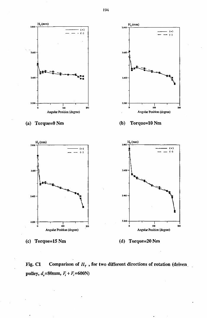
l!r(mm) 3.8(lO -,--''---------------,

---(+)

- - -(0)

3.600

3.400

3.200-4---,...-----r----,----;

o 100 200


(a) Torque=O Nm

l!r(mm) 3.8(JO ...,.:---------------,

3.600 I

3.400

--(+) __ (0)

3.200 +---,...-----r----,---i

o 100 200


(c) Torque=15 Nm

194

l!r(mm) 3.800 ,..:.--------------,

--(+)

--(0)

3.600

3.400

3.200 +---,...----,---..,.-----1

o 100 200


(b) Torque=10 Nm

!lr(mm) 3.800...,:...----------,

--(+)

- - (.)

3.600

3.400

3.200-4---..-----.----.----;

o 100 200


(d) Torque=20 Nm

Fig. Cl Comparison of Hr , for two different directions of rotation (driven.

pulley, de=80mm, F, + F,=600N)

195

Table Cl Readings of HT (mm), for two different directions

Angular T=ONm T=lONm T=15Nm T=20Nm

position

(degree)

direction + - + - + - + -

0 3.500 3.512 3.568 3.609 3.633 3.716 3.756 3.770

10 3.445 3.434 3.474 3.461 3.498 3.491 3.568 3.571

20 3.450 3.441 3.476 3.474 3.507 3.503 3.554 3.553

30 3.445 3.454 3.482 3.490 3.502 3.510 3.536 3.543

60 3.434 3.449 '3.461 3.475 3.486 3.493 3.514 3.520

90 3.424 3.433 3.447 3.455 3.463 3.467 3.480 3.483

120 3.424 3.424 3.438 3.442 3.444 3.448 3.456 3.467

150 3.420 3.425 3.417 3.414 3.424 3.421 3.436 3.439

160 3.407 3.407 3.412 3.418 3.415 3.417 3.421 3.428

170 3.392 3.413 3.384 3.400 3.382 3.400 3.386 3.397

180 3.390 3.410 3.350 3.355 3.314 3.317 3.274 3.283

196

AppendixD

Details of tests for variation of H T across the belt width at angular position 900

pulley sizes 45 mm (new belt) 80 mm (used belt)

total tension 200N 300N 200N 600N

torque (Nm) 0 4 0 6 0 8 0 23

1 3.423 3.510 3.384 3.511 2.999 3.044 2.939 3.019

2 3.419 3.504 3.380 3.505 3.001 3.050 2.935 3.017

3 3.424 3.512 3.379 3.513 3.000 3.049 2.938 3.020

4 3.417 3.511 3.376 3.511 2.997 3.043 2.942 3.022

5 3.424 3.513 3.377 3.511 2.994 3.051 2.933 3.014

6 3.424 3.505 3.382 3.506 2.997 3.045 2.939 3.018

7 3.426 3.506 3.379 3.506 3.002 3.048 2.935 3.023

8 3.423 3.509 3.384 3.508 2.993 3.049 2.941 3.014

9 3.422 3.508 3.381 3.508 2.999 3.047 2.940 3.019

10 3.420 3.503 3.380 3.504 2.998 3.046 2.938 3.020

11 3.418 3.504 3.376 3.504 2.997 3.051 2.933 3.021

12 3.425 3.504 3.384 3.505 3.001 3.047 2.940 3.016

13 3.422 3.509 3.383 3.508 3.000 3.050 2.937 3.020

1 2 3 4 5 6 7 8 9 10 11 12 13

...--_1 1 1 1 1 1 1 1 1 1 1 1 1

.,.~ HT

Documents

MECHANICAL PERFORMANCE OF V-RIBBED BELT DRIVES