Embed Size (px)
Citation preview

2
It is becoming essential that we obtain more of our energy needs from renewable sources. These include wind, wave and tidal power, all of which involve the application of fl uid mechanics. Although source of energy is free, the installation costs are high and the equipment must be designed to convert as much of it as possible into electrical power. Increasing numbers of wind turbines are being erected and proposals are under discussion to harness the tidal rise and fall in river estuaries.
Photo courtesy of iStockphoto, rotofrank, Image #4646593
Mechanical Engineering, 9780080965772, 2010, Taylor and Francis.
Principles and Applications of Fluid Mechanics
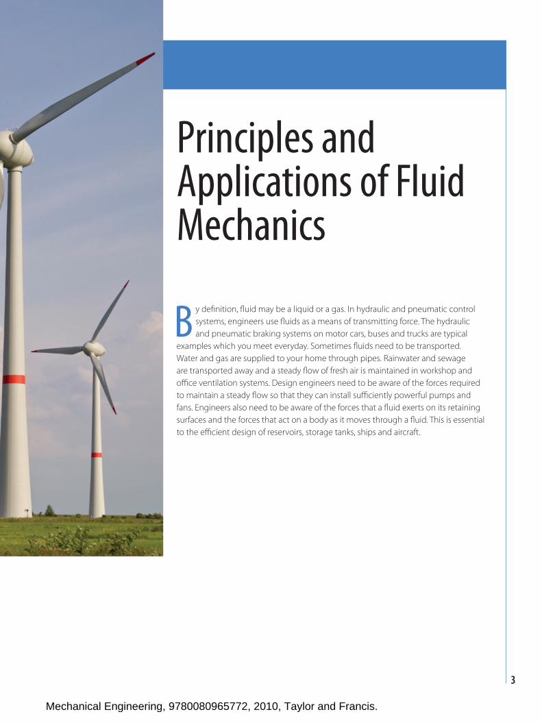
B y defi nition, fl uid may be a liquid or a gas. In hydraulic and pneumatic control systems, engineers use fl uids as a means of transmitting force. The hydraulic and pneumatic braking systems on motor cars, buses and trucks are typical
examples which you meet everyday. Sometimes fl uids need to be transported. Water and gas are supplied to your home through pipes. Rainwater and sewage are transported away and a steady fl ow of fresh air is maintained in workshop and offi ce ventilation systems. Design engineers need to be aware of the forces required to maintain a steady fl ow so that they can install suffi ciently powerful pumps and fans. Engineers also need to be aware of the forces that a fl uid exerts on its retaining surfaces and the forces that act on a body as it moves through a fl uid. This is essential to the effi cient design of reservoirs, storage tanks, ships and aircraft.
3
Mechanical Engineering, 9780080965772, 2010, Taylor and Francis.
Principles and Applications of Fluid Mechanics4
Physical Properties of Fluids
The physical properties of fl uids, whose values need to be defi ned and measured, include density, specifi c weight, relative density, dynamic and kinematic viscosity and surface tension. You will fi nd that some of these, particularly density and dynamic viscosity, recur quite often in fl uid mechanics calculations.
Density
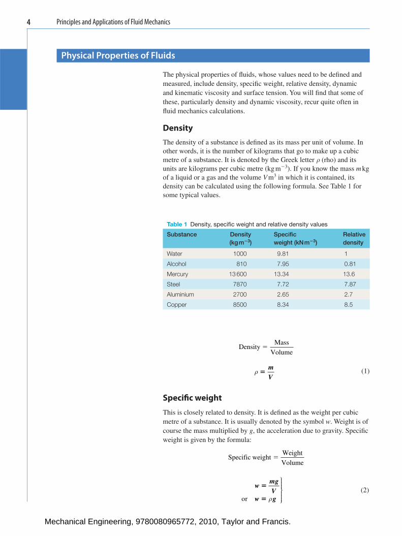
The density of a substance is defi ned as its mass per unit of volume. In other words, it is the number of kilograms that go to make up a cubic metre of a substance. It is denoted by the Greek letter ρ (rho) and its units are kilograms per cubic metre (kg m � 3 ). If you know the mass m kg of a liquid or a gas and the volume V m 3 in which it is contained, its density can be calculated using the following formula. See Table 1 for some typical values.
Table 1 Density, specifi c weight and relative density values
Substance Density (kg m�3)
Specifi c weight (kN m�3)
Relative density
Water 1000 9.81 1
Alcohol 810 7.95 0.81
Mercury 13 600 13.34 13.6
Steel 7870 7.72 7.87
Aluminium 2700 2.65 2.7
Copper 8500 8.34 8.5
Density
Mass
Volume�
ρ �
mV
(1)
Specifi c weight
This is closely related to density. It is defi ned as the weight per cubic metre of a substance. It is usually denoted by the symbol w . Weight is of course the mass multiplied by g , the acceleration due to gravity. Specifi c weight is given by the formula:
Specific weight
Weight
Volume�
wmgV
w g
�
�or ρ
⎫⎬⎪⎪⎪
⎭⎪⎪⎪
(2)
Mechanical Engineering, 9780080965772, 2010, Taylor and Francis.
Principles and Applications of Fluid Mechanics 5
The units of specifi c weight are newtons per cubic metre, or more usually kilonewtons, per cubic metre (kN m � 3 ). You might note that the density of a substance under the same conditions of temperature and pressure will be the same on the earth, the moon, Mars or anywhere out in space. The specifi c weight will however be different, as it depends on the force of gravity.
Relative density
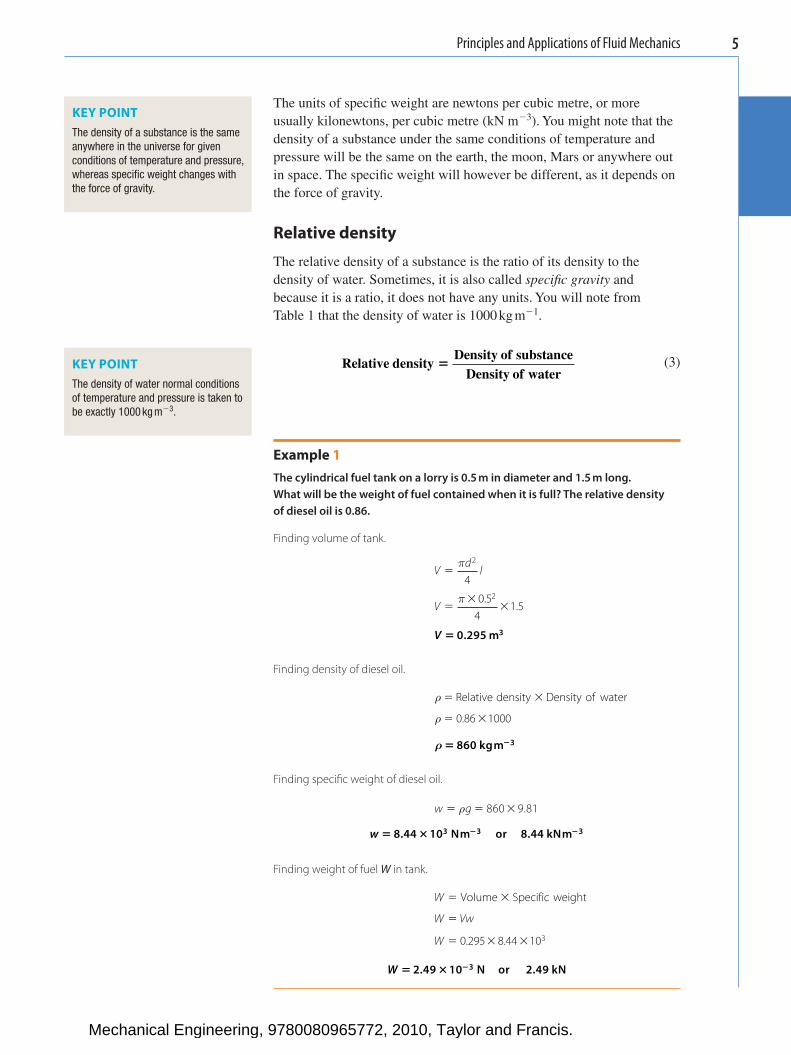
The relative density of a substance is the ratio of its density to the density of water. Sometimes, it is also called specifi c gravity and because it is a ratio, it does not have any units. You will note from Table 1 that the density of water is 1000 kg m � 1 .
Relative density
Density of substanceDensity of water
�
(3)
Example 1 The cylindrical fuel tank on a lorry is 0.5 m in diameter and 1.5 m long. What will be the weight of fuel contained when it is full? The relative density of diesel oil is 0.86.
Finding volume of tank.
Vd
l
V
�
��
�
π
π
2
2
4
0 54
1 5.
.
V � 0 295 3. m
Finding density of diesel oil.
ρ
ρ
�
�
Relative density Density of water�
�0 86 1000.
ρ � �860 kgm 3
Finding specifi c weight of diesel oil.
w g� � �ρ 860 9 81.
w � � � �8 44 10 8 443. .Nm kNm3 3or
Finding weight of fuel W in tank.
W
W Vw
W
�
�
� � �
Volume Specific weight�
0 295 8 44 103. .
W � � �2 49 10 2 493. .N kNor
KEY POINT The density of a substance is the same anywhere in the universe for given conditions of temperature and pressure, whereas specifi c weight changes with the force of gravity.
KEY POINT The density of water normal conditions of temperature and pressure is taken to be exactly 1000 kg m � 3 .
Mechanical Engineering, 9780080965772, 2010, Taylor and Francis.
Principles and Applications of Fluid Mechanics6
Viscosity
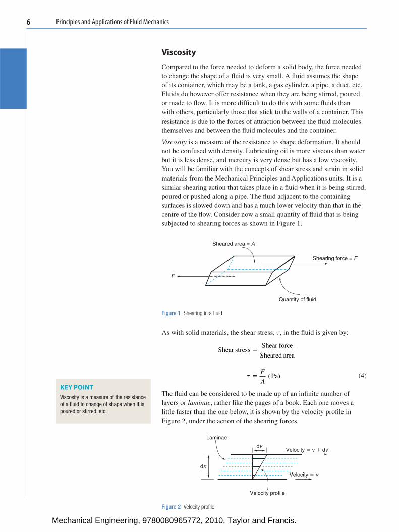
Compared to the force needed to deform a solid body, the force needed to change the shape of a fl uid is very small. A fl uid assumes the shape of its container, which may be a tank, a gas cylinder, a pipe, a duct, etc. Fluids do however offer resistance when they are being stirred, poured or made to fl ow. It is more diffi cult to do this with some fl uids than with others, particularly those that stick to the walls of a container. This resistance is due to the forces of attraction between the fl uid molecules themselves and between the fl uid molecules and the container.
Viscosity is a measure of the resistance to shape deformation. It should not be confused with density. Lubricating oil is more viscous than water but it is less dense, and mercury is very dense but has a low viscosity. You will be familiar with the concepts of shear stress and strain in solid materials from the Mechanical Principles and Applications units. It is a similar shearing action that takes place in a fl uid when it is being stirred, poured or pushed along a pipe. The fl uid adjacent to the containing surfaces is slowed down and has a much lower velocity than that in the centre of the fl ow. Consider now a small quantity of fl uid that is being subjected to shearing forces as shown in Figure 1 .
Sheared area = A
Shearing force = F
F
Quantity of fluid
Figure 1 Shearing in a fl uid
Laminae
dvVelocity � v � dv
dx
Velocity � v
Velocity profile
Figure 2 Velocity profi le
As with solid materials, the shear stress, τ , in the fl uid is given by:
Shear stress
Shear force
Sheared area�
τ �
F
A(Pa)
(4)
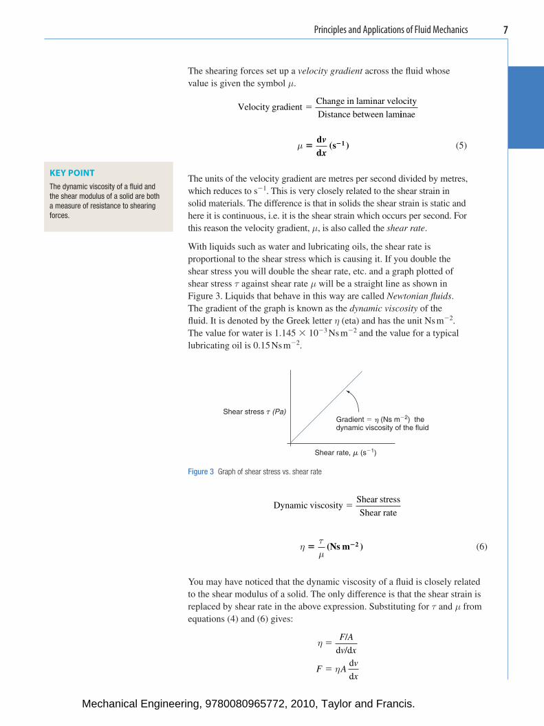
The fl uid can be considered to be made up of an infi nite number of layers or laminae , rather like the pages of a book. Each one moves a little faster than the one below, it is shown by the velocity profi le in Figure 2 , under the action of the shearing forces.
KEY POINT Viscosity is a measure of the resistance of a fl uid to change of shape when it is poured or stirred, etc.
Mechanical Engineering, 9780080965772, 2010, Taylor and Francis.
Principles and Applications of Fluid Mechanics 7
The shearing forces set up a velocity gradient across the fl uid whose value is given the symbol µ .
Velocity gradient
Change in laminar velocity
Distance between lam�
iinae
µ � �d
d(s )1v
x (5)
The units of the velocity gradient are metres per second divided by metres, which reduces to s � 1 . This is very closely related to the shear strain in solid materials. The difference is that in solids the shear strain is static and here it is continuous, i.e. it is the shear strain which occurs per second. For this reason the velocity gradient, µ , is also called the shear rate .
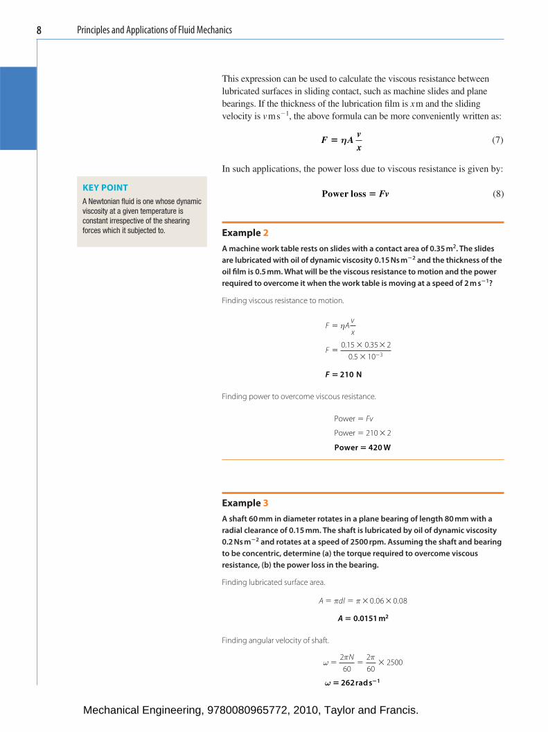
With liquids such as water and lubricating oils, the shear rate is proportional to the shear stress which is causing it. If you double the shear stress you will double the shear rate, etc. and a graph plotted of shear stress τ against shear rate µ will be a straight line as shown in Figure 3 . Liquids that behave in this way are called Newtonian fl uids . The gradient of the graph is known as the dynamic viscosity of the fl uid. It is denoted by the Greek letter η (eta) and has the unit Ns m � 2 . The value for water is 1.145 � 10 � 3 Ns m � 2 and the value for a typical lubricating oil is 0.15 Ns m � 2 .
Shear stress t (Pa)
Shear rate, m (s�1)
Gradient � h (Ns m�2) thedynamic viscosity of the fluid
Figure 3 Graph of shear stress vs. shear rate
KEY POINT The dynamic viscosity of a fl uid and the shear modulus of a solid are both a measure of resistance to shearing forces.
Dynamic viscosity
Shear stress
Shear rate�
η
τµ
� �(Ns m )2
(6)
You may have noticed that the dynamic viscosity of a fl uid is closely related to the shear modulus of a solid. The only difference is that the shear strain is replaced by shear rate in the above expression. Substituting for τ and µ from equations (4) and (6) gives:
η
η
�
�
F A
v x
F Av
x
/
d /dd
d
Mechanical Engineering, 9780080965772, 2010, Taylor and Francis.
Principles and Applications of Fluid Mechanics8
This expression can be used to calculate the viscous resistance between lubricated surfaces in sliding contact, such as machine slides and plane bearings. If the thickness of the lubrication fi lm is x m and the sliding velocity is v m s � 1 , the above formula can be more conveniently written as:
F A
vx
� η
(7)
In such applications, the power loss due to viscous resistance is given by:
Power loss � Fv (8)
Example 2 A machine work table rests on slides with a contact area of 0.35 m 2 . The slides are lubricated with oil of dynamic viscosity 0.15 Ns m � 2 and the thickness of the oil fi lm is 0.5 mm. What will be the viscous resistance to motion and the power required to overcome it when the work table is moving at a speed of 2 m s � 1 ?
Finding viscous resistance to motion.
F Avx
F
�
�� �
� �
η
0 15 0 35 20 5 10 3
. ..
F � 210 N
Finding power to overcome viscous resistance.
Power
Power
�
� �
Fv
210 2
Power W� 420
Example 3 A shaft 60 mm in diameter rotates in a plane bearing of length 80 mm with a radial clearance of 0.15 mm. The shaft is lubricated by oil of dynamic viscosity 0.2 Ns m � 2 and rotates at a speed of 2500 rpm. Assuming the shaft and bearing to be concentric, determine (a) the torque required to overcome viscous resistance, (b) the power loss in the bearing.
Finding lubricated surface area.
A dl� � � �π π 0 06 0 08. .
A � 0.0151 m2
Finding angular velocity of shaft.
ω
π π� � �
260
260
2500N
ω � �262rad s 1
KEY POINT A Newtonian fl uid is one whose dynamic viscosity at a given temperature is constant irrespective of the shearing forces which it subjected to.
Mechanical Engineering, 9780080965772, 2010, Taylor and Francis.
Principles and Applications of Fluid Mechanics 9
Finding surface speed of shaft.
v r� � �ω 262 0 03.
v � �7 86 1. m s
Finding tangential viscous resistance.
F A
vx
� �� �
� �η
0 2 0 0151 7 860 15 10 3
. . ..
F � 158 N
Finding torque required to overcome viscous resistance.
T Fr� � �158 0 03.
T � 4 74. Nm
Finding power loss in bearing.
Power loss � Fv � �158 7 86.
Power loss W kW� 1242 1 24or .
The viscosity of a substance is sometimes defi ned in a slightly different way for use in advanced fl uid mechanics calculations. It is known as kinematic viscosity , which is the ratio of dynamic viscosity and density. Kinematic viscosity is denoted by the Greek letter ν (nu) and has the unit m 2 s � 1 .
Kinematic viscosity
Dynamic viscosity
Density�
υ
ηρ
� �(m s )2 1
(9)
Non-Newtonian fl uids
As can be seen in Figure 3 , the graph of shear stress against shear rate for a Newtonian fl uid is a straight line which passes through the origin. This indicates that its viscosity does not change no matter how quickly it is sheared by stirring or pumping. There are however many fl uids which do not behave in this way and they may be broadly divided into two classes.
● Thixotropic fl uids , in which the viscosity falls as the rate of shearing increases. These are also known as shear thinning fl uids.
● Rheopectic fl uids , in which the viscosity rises as the rate of shearing increases. These are also known as shear thickening fl uids.
The graphs of shear stress τ against shear rate µ for these fl uids are as follows. They are known as rheograms . On these graphs, the ratio of shear stress to shear rate at any point on the curve is known as the apparent dynamic viscosity , η a , of the fl uid. Another way of defi ning apparent viscosity is to say that it is the gradient of a line drawn from the origin to that point on the curve. There are three common types of thixotropic, or shear thickening, fl uid. They are called Bingham plastic, pseudoplastic and Casson plastic.
KEY POINT The viscosity of thixotropic fl uids falls when they are stirred whilst the viscosity of rheopectic fl uids increases.
Mechanical Engineering, 9780080965772, 2010, Taylor and Francis.
Principles and Applications of Fluid Mechanics10
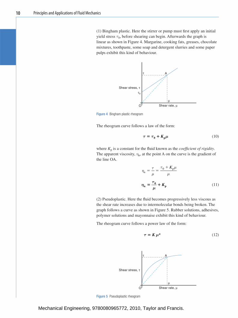
(1) Bingham plastic. Here the stirrer or pump must fi rst apply an initial yield stress τ 0 , before shearing can begin. Afterwards the graph is linear as shown in Figure 4 . Margarine , cooking fats, greases, chocolate mixtures, toothpaste, some soap and detergent slurries and some paper pulps exhibit this kind of behaviour.
τ
Shear stress, τ
A
µO Shear rate, µ
Figure 5 Pseudoplastic rheogram
τ
Shear stress, τ
A
τ0
µO Shear rate, µ
Figure 4 Bingham plastic rheogram
The rheogram curve follows a law of the form:
τ τ µ� �0 pK
(10)
where K p is a constant for the fl uid known as the coeffi cient of rigidity . The apparent viscosity, η a , at the point A on the curve is the gradient of the line OA.
η
τµ
τ µ
µa0 p
� �� K
η
τµa
0p� � K
(11)
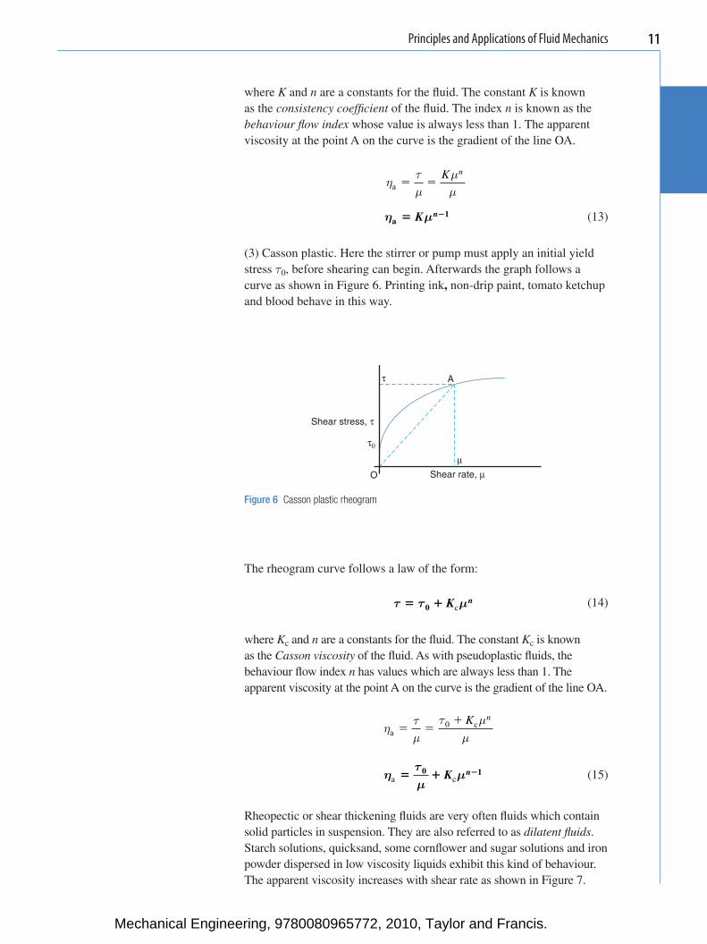
(2) Pseudoplastic. Here the fl uid becomes progressively less viscous as the shear rate increases due to intermolecular bonds being broken. The graph follows a curve as shown in Figure 5 . Rubber solutions, adhesives, polymer solutions and mayonnaise exhibit this kind of behaviour.
The rheogram curve follows a power law of the form:
τ µ� K n
(12)
Mechanical Engineering, 9780080965772, 2010, Taylor and Francis.
Principles and Applications of Fluid Mechanics 11
where K and n are a constants for the fl uid. The constant K is known as the consistency coeffi cient of the fl uid. The index n is known as the behaviour fl ow index whose value is always less than 1. The apparent viscosity at the point A on the curve is the gradient of the line OA.
η
τµ
µµa � �
K n
η µa1� �K n
(13)
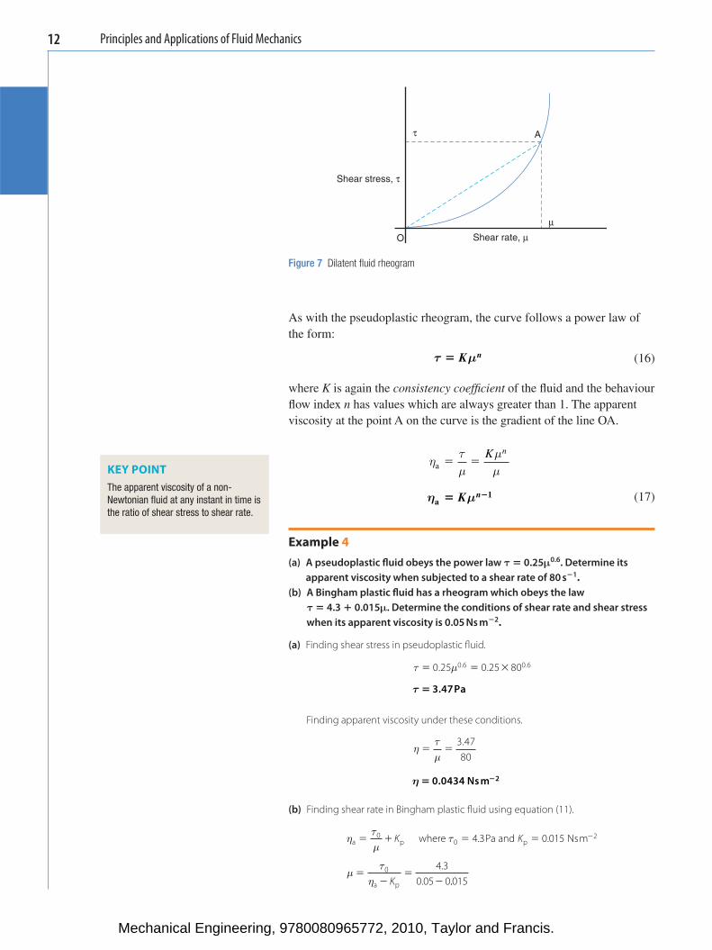
(3) Casson plastic. Here the stirrer or pump must apply an initial yield stress τ 0 , before shearing can begin. Afterwards the graph follows a curve as shown in Figure 6 . Printing ink , non-drip paint, tomato ketchup and blood behave in this way.
τ
Shear stress, τ
A
τ0
µO Shear rate, µ
Figure 6 Casson plastic rheogram
The rheogram curve follows a law of the form:
τ τ µ� �0 K nc
(14)
where K c and n are a constants for the fl uid. The constant K c is known as the Casson viscosity of the fl uid. As with pseudoplastic fl uids, the behaviour fl ow index n has values which are always less than 1. The apparent viscosity at the point A on the curve is the gradient of the line OA.
η
τµ
τ µµa
0 c� �� K n
η
τµ
µa c� � �0 1K n
(15)
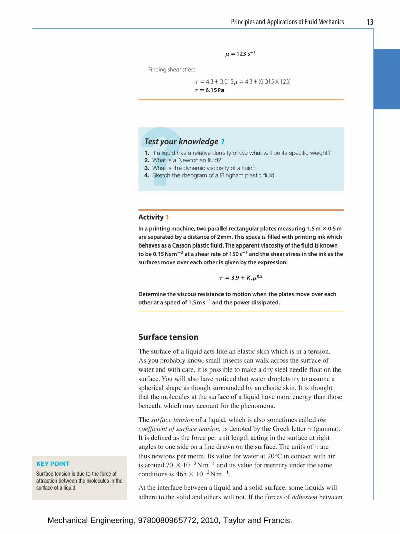
Rheopectic or shear thickening fl uids are very often fl uids which contain solid particles in suspension. They are also referred to as dilatent fl uids . Starch solutions, quicksand, some cornfl ower and sugar solutions and iron powder dispersed in low viscosity liquids exhibit this kind of behaviour. The apparent viscosity increases with shear rate as shown in Figure 7 .
Mechanical Engineering, 9780080965772, 2010, Taylor and Francis.
Principles and Applications of Fluid Mechanics12
τ
Shear stress, τ
A
µ
O Shear rate, µ
Figure 7 Dilatent fl uid rheogram
As with the pseudoplastic rheogram, the curve follows a power law of the form:
τ µ� K n
(16)
where K is again the consistency coeffi cient of the fl uid and the behaviour fl ow index n has values which are always greater than 1. The apparent viscosity at the point A on the curve is the gradient of the line OA.
η
τµ
µµa � �
K n
η µa1� �K n
(17)
Example 4 (a) A pseudoplastic fl uid obeys the power law τ � 0.25 µ 0.6 . Determine its
apparent viscosity when subjected to a shear rate of 80 s � 1 . (b) A Bingham plastic fl uid has a rheogram which obeys the law
τ � 4.3 � 0.015 µ . Determine the conditions of shear rate and shear stress when its apparent viscosity is 0.05 Ns m � 2 .
(a) Finding shear stress in pseudoplastic fl uid.
τ µ� � �0 25 0 25 800 6 0 6. .. .
τ � 3 47. Pa
Finding apparent viscosity under these conditions.
η
τµ
� �3 4780.
η � �0 0434 2. Ns m
(b) Finding shear rate in Bingham plastic fl uid using equation (11).
ητµ
τ
µτ
η
a0
p 0 p
0
a p
where Pa and Nsm� � � �
��
��
�K K
K
4 3 0 015
4 30 05 0
2. .
.. ..015
KEY POINT The apparent viscosity of a non-Newtonian fl uid at any instant in time is the ratio of shear stress to shear rate.
Mechanical Engineering, 9780080965772, 2010, Taylor and Francis.
Principles and Applications of Fluid Mechanics 13
µ � �123 1s
Finding shear stress.
τ µ� � � � �4 3 0 015 4 3 0 015 123. . . . ( ) τ � 6 15. Pa
? Test your knowledge 1 1. If a liquid has a relative density of 0.9 what will be its specifi c weight? 2. What is a Newtonian fl uid? 3. What is the dynamic viscosity of a fl uid? 4. Sketch the rheogram of a Bingham plastic fl uid.
Activity 1 In a printing machine, two parallel rectangular plates measuring 1.5 m � 0.5 m are separated by a distance of 2 mm. This space is fi lled with printing ink which behaves as a Casson plastic fl uid. The apparent viscosity of the fl uid is known to be 0.15 Ns m � 2 at a shear rate of 150 s � 1 and the shear stress in the ink as the surfaces move over each other is given by the expression:
τ µ� �3.9 0.5Kc
Determine the viscous resistance to motion when the plates move over each other at a speed of 1.5 m s � 1 and the power dissipated.
Surface tension
The surface of a liquid acts like an elastic skin which is in a tension. As you probably know, small insects can walk across the surface of water and with care, it is possible to make a dry steel needle fl oat on the surface. You will also have noticed that water droplets try to assume a spherical shape as though surrounded by an elastic skin. It is thought that the molecules at the surface of a liquid have more energy than those beneath, which may account for the phenomena.
The surface tension of a liquid, which is also sometimes called the coeffi cient of surface tension , is denoted by the Greek letter γ (gamma). It is defi ned as the force per unit length acting in the surface at right angles to one side on a line drawn on the surface. The units of γ are thus newtons per metre. Its value for water at 20°C in contact with air is around 70 � 10 � 3 N m � 1 and its value for mercury under the same conditions is 465 � 10 � 2 N m � 1 .
At the interface between a liquid and a solid surface, some liquids will adhere to the solid and others will not. If the forces of adhesion between
KEY POINT Surface tension is due to the force of attraction between the molecules in the surface of a liquid.
Mechanical Engineering, 9780080965772, 2010, Taylor and Francis.
Principles and Applications of Fluid Mechanics14
the liquid molecules and those of the solid are greater than the forces of cohesion between the liquid molecules themselves, the liquid will ‘ wet ’ the solid and vice versa. Water and alcohol will readily adhere to clean glass whereas mercury will not.
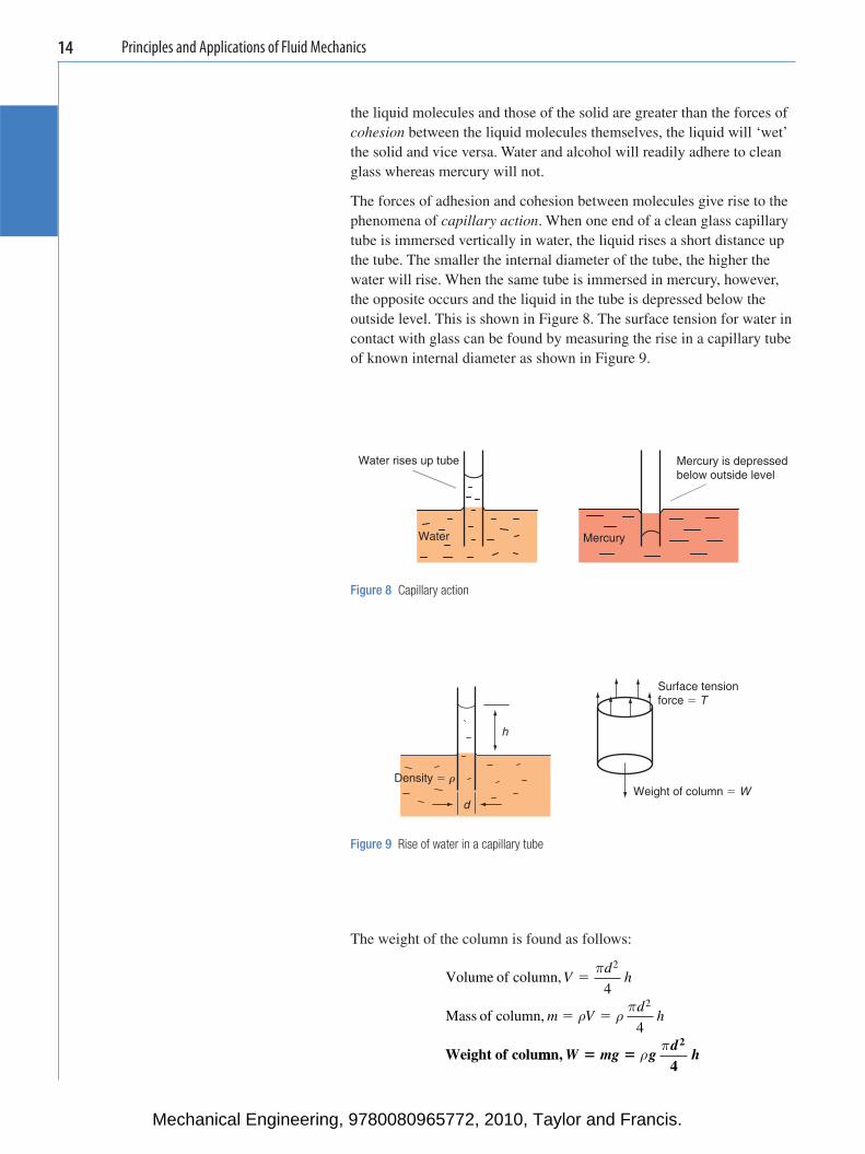
The forces of adhesion and cohesion between molecules give rise to the phenomena of capillary action . When one end of a clean glass capillary tube is immersed vertically in water, the liquid rises a short distance up the tube. The smaller the internal diameter of the tube, the higher the water will rise. When the same tube is immersed in mercury, however, the opposite occurs and the liquid in the tube is depressed below the outside level. This is shown in Figure 8 . The surface tension for water in contact with glass can be found by measuring the rise in a capillary tube of known internal diameter as shown in Figure 9 .
Water rises up tube Mercury is depressedbelow outside level
Water Mercury
Figure 8 Capillary action
Surface tensionforce � T
h
Density � rWeight of column � W
d
Figure 9 Rise of water in a capillary tube
The weight of the column is found as follows:
Volume of column,
Mass of column,
Vd
h
m Vd
h
�
� �
π
ρ ρπ
2
24
4
Weight of colummn,4
2W mg g
dh� � ρ
π
Mechanical Engineering, 9780080965772, 2010, Taylor and Francis.
Principles and Applications of Fluid Mechanics 15
If γ is the surface tension force per metre, the upward surface tension force is given by:
Surface tension, dT � π γ
Equating these two expressions enables γ to be found.
Surface tension force, Weight,T W
d gd
h
�
�π γ ρπ 2
4
γ ρ� g
dh
4 (18)
In deriving the above formula it is assumed that the meniscus at the top of the column meets the glass vertically around its edge. This is in fact very close to being the case for water and alcohol provided that the glass is clean.
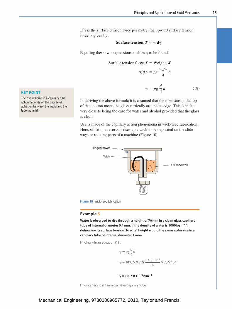
Use is made of the capillary action phenomena in wick-feed lubrication. Here, oil from a reservoir rises up a wick to be deposited on the slide-ways or rotating parts of a machine ( Figure 10 ).
KEY POINT The rise of liquid in a capillary tube action depends on the degree of adhesion between the liquid and the tube material.
Oil reservoir
Wick
Hinged cover
Figure 10 Wick-feed lubrication
Example 5 Water is observed to rise through a height of 70 mm in a clean glass capillary tube of internal diameter 0.4 mm. If the density of water is 1000 kg m � 3 , determine its surface tension. To what height would the same water rise in a capillary tube of internal diameter 1 mm?
Finding γ from equation (18).
γ ρ
γ
�
� � ��
� ��
�
gd
h4
1000 9 810 4 10
470 10
33.
.
γ � � � �68 7 10 3 1. Nm
Finding height in 1 mm diameter capillary tube.
Mechanical Engineering, 9780080965772, 2010, Taylor and Francis.
Principles and Applications of Fluid Mechanics16
γ ρ
γρ
�
�
�� �
� � �
�
�
g h
hgd
h
d4
4
4 68.7 101000 9.81 1 10
3
3
h � 0 028 28. m mmor
Laminar and turbulent fl ow
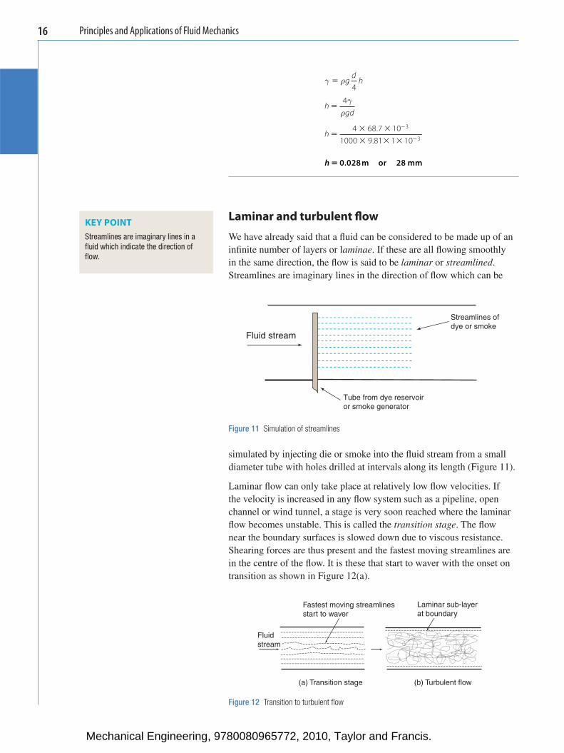
We have already said that a fl uid can be considered to be made up of an infi nite number of layers or l aminae . If these are all fl owing smoothly in the same direction, the fl ow is said to be laminar or streamlined . Streamlines are imaginary lines in the direction of fl ow which can be
KEY POINT Streamlines are imaginary lines in a fl uid which indicate the direction of fl ow.
Streamlines of dye or smoke
Fluid stream
Tube from dye reservoiror smoke generator
Figure 11 Simulation of streamlines
simulated by injecting die or smoke into the fl uid stream from a small diameter tube with holes drilled at intervals along its length ( Figure 11 ).
Laminar fl ow can only take place at relatively low fl ow velocities. If the velocity is increased in any fl ow system such as a pipeline, open channel or wind tunnel, a stage is very soon reached where the laminar fl ow becomes unstable. This is called the transition stage . The fl ow near the boundary surfaces is slowed down due to viscous resistance. Shearing forces are thus present and the fastest moving streamlines are in the centre of the fl ow. It is these that start to waver with the onset on transition as shown in Figure 12(a) .
Fastest moving streamlines start to waver
Laminar sub-layerat boundary
Fluidstream
(a) Transition stage (b) Turbulent flow
Figure 12 Transition to turbulent fl ow
Mechanical Engineering, 9780080965772, 2010, Taylor and Francis.
Principles and Applications of Fluid Mechanics 17
As the fl ow velocity increases beyond the transition stage, the streamlines disintegrate and the fl ow then consists of a random eddying motion. It is then said to be fully turbulent as shown in Figure 12(b) . Even with turbulent fl ow, however, there remains a thin laminar sub-layer adjacent to the system boundary where the fl ow velocity is retarded by viscous resistance. It is across this sub-layer that most of the shearing action in the fl uid takes place. A body placed in the fl uid stream experiences this as a drag force. To be more precise, it is known as skin friction drag which will be described in more detail later.
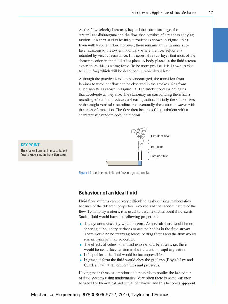
Although the practice is not to be encouraged, the transition from laminar to turbulent fl ow can be observed in the smoke rising from a lit cigarette as shown in Figure 13 . The smoke contains hot gases that accelerate as they rise. The stationary air surrounding them has a retarding effect that produces a shearing action. Initially the smoke rises with straight vertical streamlines but eventually these start to waver with the onset of transition. The fl ow then becomes fully turbulent with a characteristic random eddying motion.
KEY POINT The change from laminar to turbulent fl ow is known as the transition stage.
Turbulent flow
Transition
Laminar flow
Figure 13 Laminar and turbulent fl ow in cigarette smoke
Behaviour of an ideal fl uid
Fluid fl ow systems can be very diffi cult to analyse using mathematics because of the different properties involved and the random nature of the fl ow. To simplify matters, it is usual to assume that an ideal fl uid exists. Such a fl uid would have the following properties:
● The dynamic viscosity would be zero. As a result there would be no shearing at boundary surfaces or around bodies in the fl uid stream. There would be no retarding forces or drag forces and the fl ow would remain laminar at all velocities.
● The effects of cohesion and adhesion would be absent, i.e. there would be no surface tension in the fl uid and no capillary action.
● In liquid form the fl uid would be incompressible. ● In gaseous form the fl uid would obey the gas laws (Boyle’s law and
Charles ’ law) at all temperatures and pressures.
Having made these assumptions it is possible to predict the behaviour of fl uid systems using mathematics. Very often there is some variance between the theoretical and actual behaviour, and this becomes apparent
Mechanical Engineering, 9780080965772, 2010, Taylor and Francis.
Principles and Applications of Fluid Mechanics18
when the predictions are tested experimentally. Nevertheless, the assumption of ideal fl uid behaviour gives us a starting point from which we can develop formulae. Correction factors can then be applied in the light of experimental evidence to make the theoretical predictions correlate more nearly with the actual behaviour.
Fluid fl ow calculations contain many of these experimentally derived correction factors. They are sometimes disparagingly known as ‘ fudge ’ factors, but more correctly they are known as correction coeffi cients. Typical examples are velocity coeffi cients, discharge coeffi cients and drag coeffi cients. Fortunately, water and air behave surprisingly close to the ideal fl uid model in many respects and there is not too much of a difference between their actual and predicted behaviour.
KEY POINT The effects of viscosity and surface tension would be absent in an ideal fl uid. ? Test your knowledge 2
1. How is the coeffi cient of surface tension defi ned? 2. What is capillary action? 3. What are streamlines? 4. What name is given to the change from laminar to turbulent fl ow? 5. What would be the properties of an ideal fl uid?
Activity 2 A glass microscope slide of length 60 mm and thickness 2 mm is suspended from a sensitive balance with its lower edge touching the surface of a beaker of water. The beaker is slowly lowered and at the point where the slide breaks free of the water the balance reading is 11.13 g. The balance reading then falls to 10.25 g, which is the mass of the slide. What is the surface tension coeffi cient for the water?
Hydrostatic Systems
Hydrostatic systems are those in which the fl uid is at rest or in which the movements of the fl uid are relatively small. Pressure measuring devices such as piezometers, manometers and barometers are examples of this type of system as are fl oating and immersed bodies which experience up-thrust and fl uid pressure. In other types of hydrostatic system, the fl uid is used as a means of transmitting force. Hydraulic jacks, presses and breaking systems are examples of this category.
Hydrostatic pressure
Pressure is the intensity of the force acting on a surface and is measured in pascals (Pa). A pascal is defi ned as a force of 1 N which acts evenly and at right angles over a surface of area 1 m 2 . This is rather a small unit for practical purposes and pressure is more generally measured in kPa or
Mechanical Engineering, 9780080965772, 2010, Taylor and Francis.
Principles and Applications of Fluid Mechanics 19
even MPa. Although the pascal is the standard SI unit of pressure, there are others in common use. One of these is the ‘ bar ’ which is widely used for measuring high pressures in steam plant and industrial processes.
1 bar 100 000 Pa 100 kPa� or
To convert from bars to Pa multiply byy or100 000 105
The ‘ bar ’ gets its name from barometric or atmospheric pressure which is approximately equal to 1 bar.
Standard atmospheric pressure 101 325 Pa or 101 325 kPaor 1 01325 b
� .. aar
It should be remembered that manometers and mechanical pressure gauges do not usually measure the total or absolute pressure inside a containing vessel. Instead they measure the difference between the pressure inside and atmospheric pressure on the outside. This is known as gauge pressure . If the absolute pressure is required, atmospheric pressure must be added to it.
i.e. Absolute pressure Guage pressureAtmospheric pressure
� �
In fl uid mechanics calculations it is generally the gauge pressure that is used and unless you are told otherwise, any pressure values which you are given can be assumed to be gauge pressures.
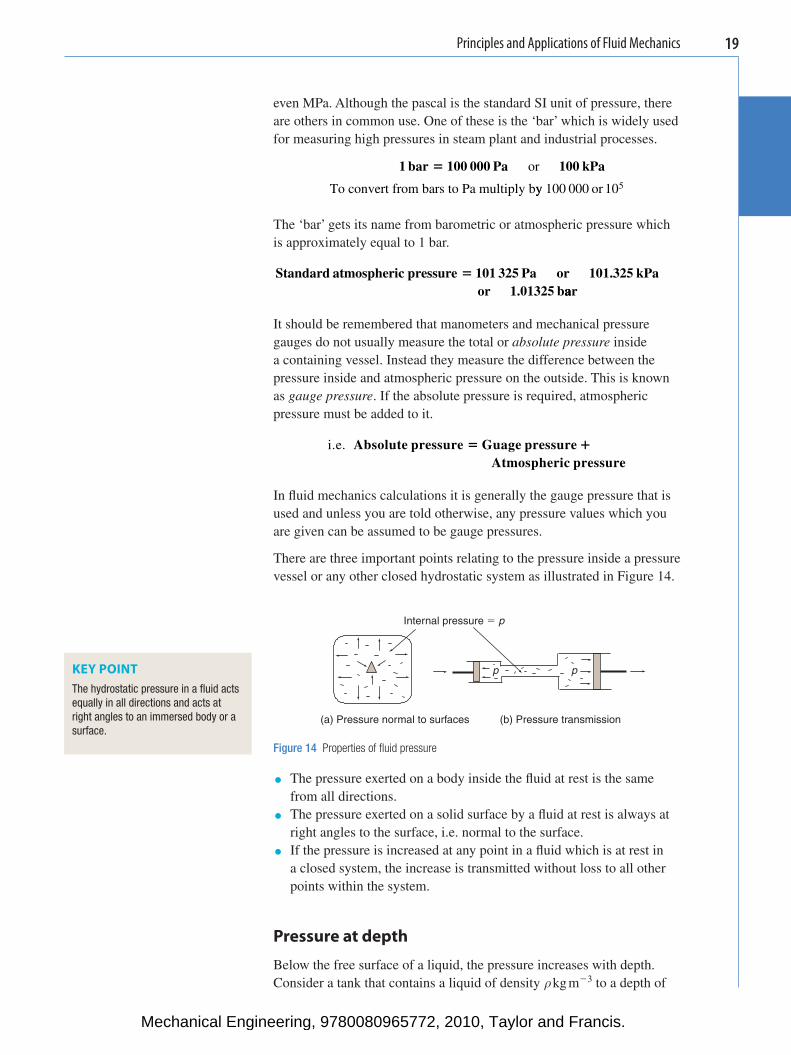
There are three important points relating to the pressure inside a pressure vessel or any other closed hydrostatic system as illustrated in Figure 14 .
Internal pressure � p
p p
(a) Pressure normal to surfaces (b) Pressure transmission
Figure 14 Properties of fl uid pressure
● The pressure exerted on a body inside the fl uid at rest is the same from all directions.
● The pressure exerted on a solid surface by a fl uid at rest is always at right angles to the surface, i.e. normal to the surface.
● If the pressure is increased at any point in a fl uid which is at rest in a closed system, the increase is transmitted without loss to all other points within the system.
Pressure at depth
Below the free surface of a liquid, the pressure increases with depth. Consider a tank that contains a liquid of density ρ kg m � 3 to a depth of
KEY POINT The hydrostatic pressure in a fl uid acts equally in all directions and acts at right angles to an immersed body or a surface.
Mechanical Engineering, 9780080965772, 2010, Taylor and Francis.
Principles and Applications of Fluid Mechanics20
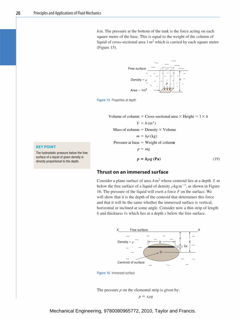
h m. The pressure at the bottom of the tank is the force acting on each square metre of the base. This is equal to the weight of the column of liquid of cross-sectional area 1 m 2 which is carried by each square metre ( Figure 15 ).
Free surface
Density � r hp
Area � 1m2
Figure 15 Properties at depth
Volume of column Cross-sectional area Height
m
Mass of
� � � �
�
13
h
V h ( )
ccolumn Density Volume
kg
Pressure at base Weight of colum
� �
�
�
m h� ( )
nn
p mg�
p h g� ρ (Pa) (19)
Thrust on an immersed surface
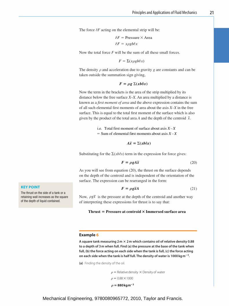
Consider a plane surface of area A m 2 whose centroid lies at a depth x m below the free surface of a liquid of density ρ kg m � 3 , as shown in Figure 16 . The pressure of the liquid will exert a force F on the surface. We will show that it is the depth of the centroid that determines this force and that it will be the same whether the immersed surface is vertical, horizontal or inclined at some angle. Consider now a thin strip of length b and thickness δ x which lies at a depth x below the free surface.
KEY POINT The hydrostatic pressure below the free surface of a liquid of given density is directly proportional to the depth.
X Free surface X
xDensity � r b x
δx
Centroid of surface
Figure 16 Immersed surface
The pressure p on the elemental strip is given by:
p x g� ρ
Mechanical Engineering, 9780080965772, 2010, Taylor and Francis.
Principles and Applications of Fluid Mechanics 21
The force δ F acting on the elemental strip will be:
δ
δ ρ δ
F
F x gb x
� �
�
Pressure Area
Now the total force F will be the sum of all these small forces.
F x gb x� �( )ρ δ
The density ρ and acceleration due to gravity g are constants and can be taken outside the summation sign giving,
F g xb x� ρ δ�( )
Now the term in the brackets is the area of the strip multiplied by its distance below the free surface X–X . An area multiplied by a distance is known as a fi rst moment of area and the above expression contains the sum of all such elemental fi rst moments of area about the axis X–X in the free surface. This is equal to the total fi rst moment of the surface which is also given by the product of the total area A and the depth of the centroid x.
i.e. Total first moment of surface about axisSum of elemental fi
X X–� rrst moments about axis X X–
Ax xb x� �( )d
Substituting for the � ( xb δ x ) term in the expression for force gives:
F gAx� ρ
(20)
As you will see from equation (20), the thrust on the surface depends on the depth of the centroid and is independent of the orientation of the surface. The expression can be rearranged in the form:
F gxA� ρ (21)
Now, ρgx is the pressure at the depth of the centroid and another way of interpreting these expressions for thrust is to say that:
Thrust Pressure at centroid Immersed surface area� �
Example 6 A square tank measuring 2 m � 2 m which contains oil of relative density 0.88 to a depth of 3 m when full. Find (a) the pressure at the base of the tank when full, (b) the force acting on each side when the tank is full, (c) the force acting on each side when the tank is half full. The density of water is 1000 kg m � 3 .
(a) Finding the density of the oil.
ρ
ρ
� �
�
Relative density Density of water
0 88 1000. �
ρ � �880 3kgm
KEY POINT The thrust on the side of a tank or a retaining wall increases as the square of the depth of liquid contained.
Mechanical Engineering, 9780080965772, 2010, Taylor and Francis.
Principles and Applications of Fluid Mechanics22
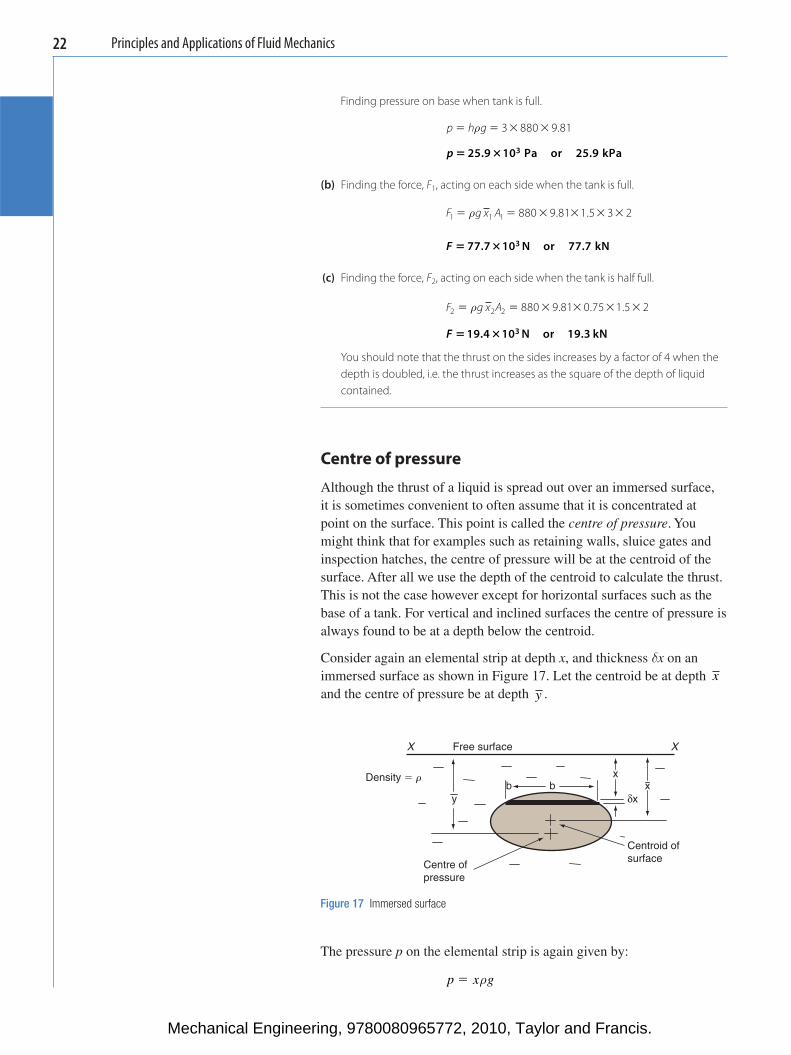
Finding pressure on base when tank is full.
p h g� � � �ρ 3 880 9 81.
p � �25 9 10 25 93. .Pa kPaor
(b) Finding the force, F 1 , acting on each side when the tank is full.
F g x A1 1 1 880 9 81 1 5 3 2� � � � � �ρ . .
F � �77 7 10 7 73. .N kNor 7
(c) Finding the force, F 2 , acting on each side when the tank is half full.
F g x A2 2 2 880 9 81 0 75 1 5 2� � � � � �ρ . . .
F � �19 4 10 19 33. .N or kN You should note that the thrust on the sides increases by a factor of 4 when the depth is doubled, i.e. the thrust increases as the square of the depth of liquid contained.
Centre of pressure
Although the thrust of a liquid is spread out over an immersed surface, it is sometimes convenient to often assume that it is concentrated at point on the surface. This point is called the centre of pressure . You might think that for examples such as retaining walls, sluice gates and inspection hatches, the centre of pressure will be at the centroid of the surface. After all we use the depth of the centroid to calculate the thrust. This is not the case however except for horizontal surfaces such as the base of a tank. For vertical and inclined surfaces the centre of pressure is always found to be at a depth below the centroid.
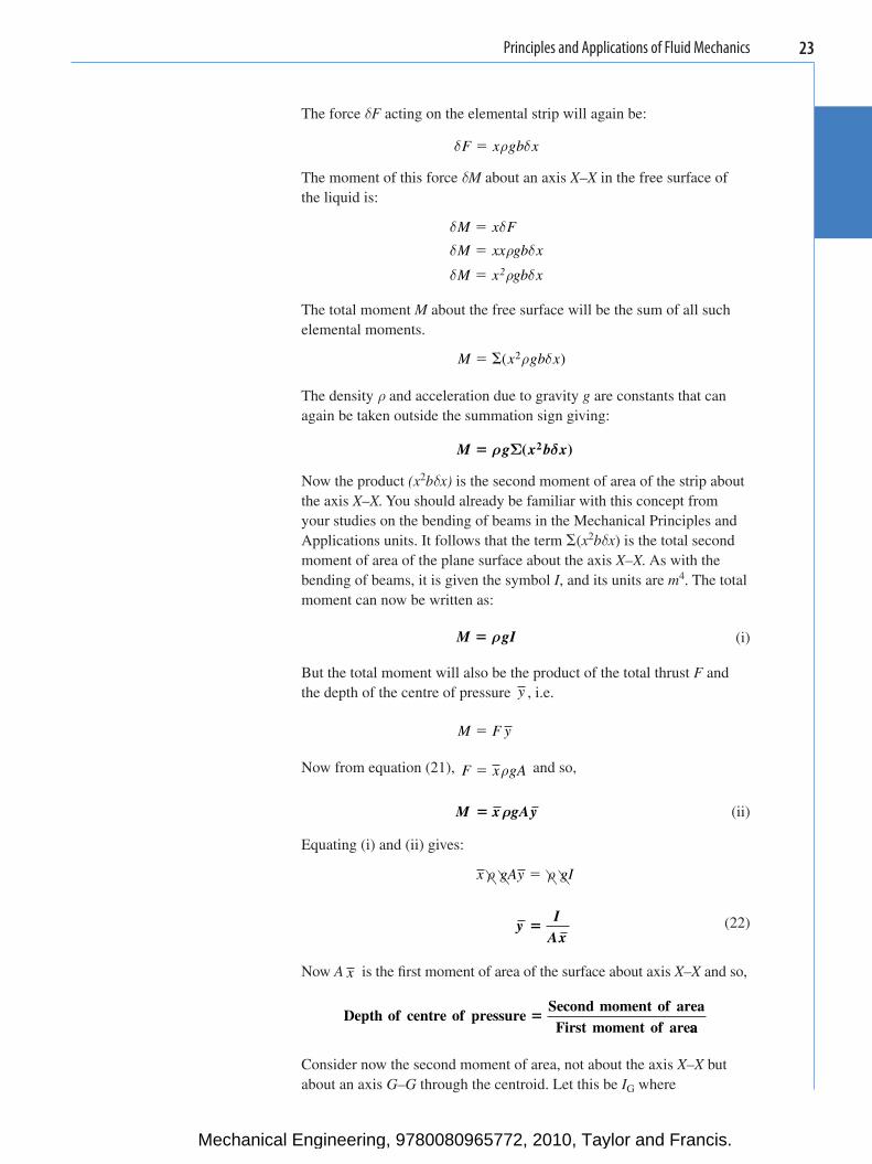
Consider again an elemental strip at depth x , and thickness δ x on an immersed surface as shown in Figure 17 . Let the centroid be at depth x and the centre of pressure be at depth y .
X Free surface X
xb x
y δx
Centroid of surface
Centre ofpressure
Density � rb
Figure 17 Immersed surface
The pressure p on the elemental strip is again given by:
p x g� ρ
Mechanical Engineering, 9780080965772, 2010, Taylor and Francis.
Principles and Applications of Fluid Mechanics 23
The force δ F acting on the elemental strip will again be:
δ ρ δF x gb x�
The moment of this force δ M about an axis X–X in the free surface of the liquid is:
δ δ
δ ρ δ
δ ρ δ
M x F
M xx gb x
M x gb x
�
�
� 2
The total moment M about the free surface will be the sum of all such elemental moments.
M x gb x� �( )2ρ δ
The density ρ and acceleration due to gravity g are constants that can again be taken outside the summation sign giving:
M g x b x� ρ δΣ( )2
Now the product (x 2 b δ x) is the second moment of area of the strip about the axis X–X. You should already be familiar with this concept from your studies on the bending of beams in the Mechanical Principles and Applications units. It follows that the term � ( x 2 b δ x ) is the total second moment of area of the plane surface about the axis X–X. As with the bending of beams, it is given the symbol I , and its units are m 4 . The total moment can now be written as:
M gI� ρ
(i)
But the total moment will also be the product of the total thrust F and the depth of the centre of pressure y , i.e.
M F y�
Now from equation (21), F gA� xρ and so,
M x gAy� ρ (ii)
Equating (i) and (ii) gives:
x gAy gIρ ρ�
y
IAx
�
(22)
Now A x is the fi rst moment of area of the surface about axis X–X and so,
Depth of centre of pressure
Second moment of areaFirst moment of are
�aa
Consider now the second moment of area, not about the axis X–X but about an axis G–G through the centroid. Let this be I G where
Mechanical Engineering, 9780080965772, 2010, Taylor and Francis.
Principles and Applications of Fluid Mechanics24
I AkG � 2
where k is known as the radius of gyration of the area, about the axis through its centroid. You might also remember from the Mechanical Principles and Applications units that this is a root mean square radius. What is required in equation (22) however is the second moment of area of the surface about the axis X–X and this can be obtained using the parallel axis theorem, i.e.
I I Ax
I Ak Ax
� �
� �G
2
2 2
Substituting for I in equation (22) gives:
y
Ak Ax
Ax�
�2 2
y
kx
x� �2
(23)
This shows that the centre of pressure of a vertical or inclined plane surface is always below its centroid by a distance equal to k x2 / . Eventually as the depth of immersion increases k x2 0/ → and the centre of pressure tends to become coincident with the centroid of the surface.
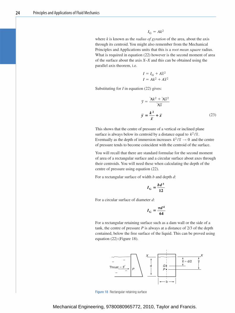
You will recall that there are standard formulae for the second moment of area of a rectangular surface and a circular surface about axes through their centroids. You will need these when calculating the depth of the centre of pressure using equation (22).
For a rectangular surface of width b and depth d :
I
bdG �
3
12
For a circular surface of diameter d :
I
dG �
π 4
64
For a rectangular retaining surface such as a dam wall or the side of a tank, the centre of pressure P is always at a distance of 2/3 of the depth contained, below the free surface of the liquid. This can be proved using equation (22) ( Figure 18 ).
x � d/2 y
X X
GPP
dThrust � F
b
Figure 18 Rectangular retaining surface
Mechanical Engineering, 9780080965772, 2010, Taylor and Francis.
Principles and Applications of Fluid Mechanics 25
Using the parallel axis theorem, the second moment of area I of the wetted surface about the axis X–X is given by:
I I Ax
Ibd
bdd bd bd
Ibd bd b
� �
� � � �
��
�
G2
3 2 3 3
3 3
12 2 12 4
3
12
4
⎛
⎝⎜⎜⎜
⎞
⎠⎟⎟⎟⎟
dd3
12
Ibd
�3
3
From equation (22),
yI
Ax
ybd
bdd bd
bd
�
� �3 3
23 2 3
⎛⎝⎜⎜⎜
⎞⎠⎟⎟⎟⎟
2
y d�
23
(24)
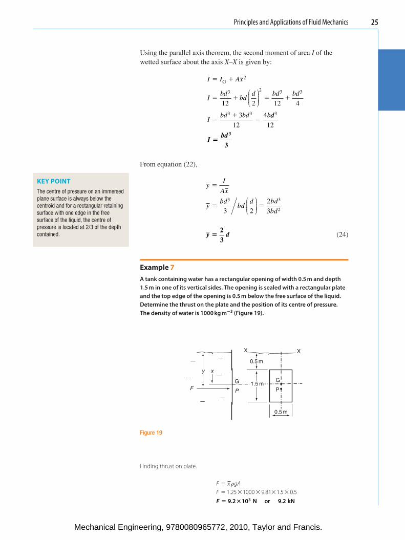
Example 7 A tank containing water has a rectangular opening of width 0.5 m and depth 1.5 m in one of its vertical sides. The opening is sealed with a rectangular plate and the top edge of the opening is 0.5 m below the free surface of the liquid. Determine the thrust on the plate and the position of its centre of pressure. The density of water is 1000 kg m � 3 ( Figure 19 ).
KEY POINT The centre of pressure on an immersed plane surface is always below the centroid and for a rectangular retaining surface with one edge in the free surface of the liquid, the centre of pressure is located at 2/3 of the depth contained.
F
0.5 m
G
P
G
P
X X
1.5 m
xy
0.5 m
Figure 19
Finding thrust on plate.
F x gAF
�
� � � �
ρ1 25 1000 9 81 1 5 0 5. . . .�
F � �9.2 10 N or 9.2 kN3
Mechanical Engineering, 9780080965772, 2010, Taylor and Francis.
Principles and Applications of Fluid Mechanics26
Finding second moment of area about axis X–X .
I I Ax
Ibd
bd
I
� �
� �
��
� � �
G2
32
32
12
0 5 1 512
0 5 1 5 1 25
x
. .. . .
⎛
⎝⎜⎜⎜⎜
⎞
⎠⎟⎟⎟⎟ (( )
I � 1.31 m4
Finding depth of centre of pressure.
yI
Ax
y
�
�� �
1 311 5 0 5 1 25
.. . .
y 1.4 m�
i.e. the centre of pressure is 0.15 m or 150 mm below the centroid of the plate.
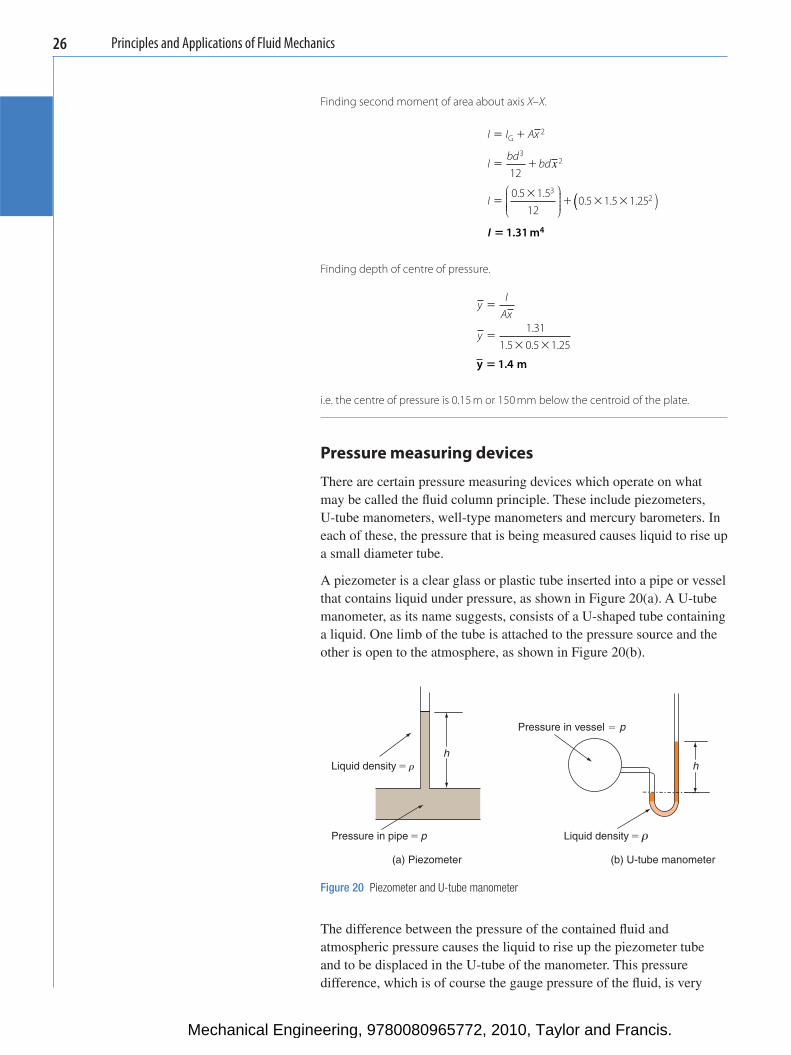
Pressure measuring devices
There are certain pressure measuring devices which operate on what may be called the fl uid column principle. These include piezometers, U-tube manometers, well-type manometers and mercury barometers. In each of these, the pressure that is being measured causes liquid to rise up a small diameter tube.
A piezometer is a clear glass or plastic tube inserted into a pipe or vessel that contains liquid under pressure, as shown in Figure 20(a) . A U-tube manometer, as its name suggests, consists of a U-shaped tube containing a liquid. One limb of the tube is attached to the pressure source and the other is open to the atmosphere, as shown in Figure 20(b) .
Pressure in vessel � p
hLiquid density � r h
Pressure in pipe � p Liquid density � r
(a) Piezometer (b) U-tube manometer
Figure 20 Piezometer and U-tube manometer
The difference between the pressure of the contained fl uid and atmospheric pressure causes the liquid to rise up the piezometer tube and to be displaced in the U-tube of the manometer. This pressure difference, which is of course the gauge pressure of the fl uid, is very
Mechanical Engineering, 9780080965772, 2010, Taylor and Francis.
Principles and Applications of Fluid Mechanics 27
often expressed directly in millimetres, e.g., mm H 2 O if it is water, or mm Hg for U-tube manometers containing mercury. Its value may also be calculated in pascals using equation (19).
i.e. p h g� ρ (Pa)
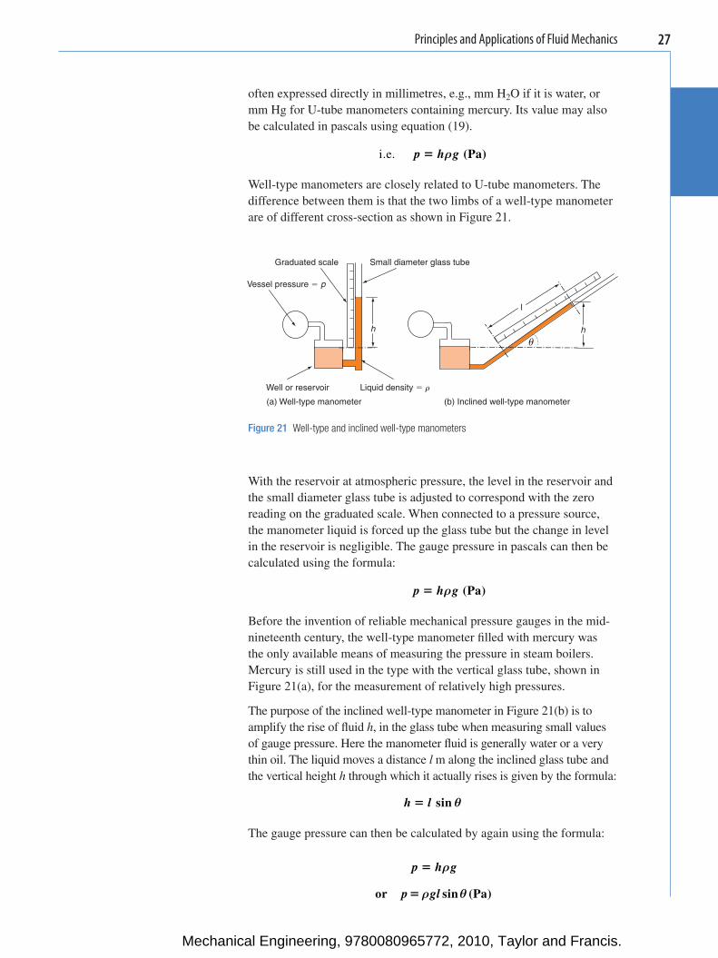
Well-type manometers are closely related to U-tube manometers. The difference between them is that the two limbs of a well-type manometer are of different cross-section as shown in Figure 21 .
Graduated scale Small diameter glass tube
Vessel pressure � p
l
h h
Well or reservoir
(a) Well-type manometer (b) Inclined well-type manometer
Liquid density � r
u
Figure 21 Well-type and inclined well-type manometers
With the reservoir at atmospheric pressure, the level in the reservoir and the small diameter glass tube is adjusted to correspond with the zero reading on the graduated scale. When connected to a pressure source, the manometer liquid is forced up the glass tube but the change in level in the reservoir is negligible. The gauge pressure in pascals can then be calculated using the formula:
p h g� ρ (Pa)
Before the invention of reliable mechanical pressure gauges in the mid-nineteenth century, the well-type manometer fi lled with mercury was the only available means of measuring the pressure in steam boilers. Mercury is still used in the type with the vertical glass tube, shown in Figure 21(a) , for the measurement of relatively high pressures.
The purpose of the inclined well-type manometer in Figure 21(b) is to amplify the rise of fl uid h , in the glass tube when measuring small values of gauge pressure. Here the manometer fl uid is generally water or a very thin oil. The liquid moves a distance l m along the inclined glass tube and the vertical height h through which it actually rises is given by the formula:
h l� sin θ
The gauge pressure can then be calculated by again using the formula:
p h g� ρ
or sin (Pa)p gl� ρ θ
Mechanical Engineering, 9780080965772, 2010, Taylor and Francis.
Principles and Applications of Fluid Mechanics28
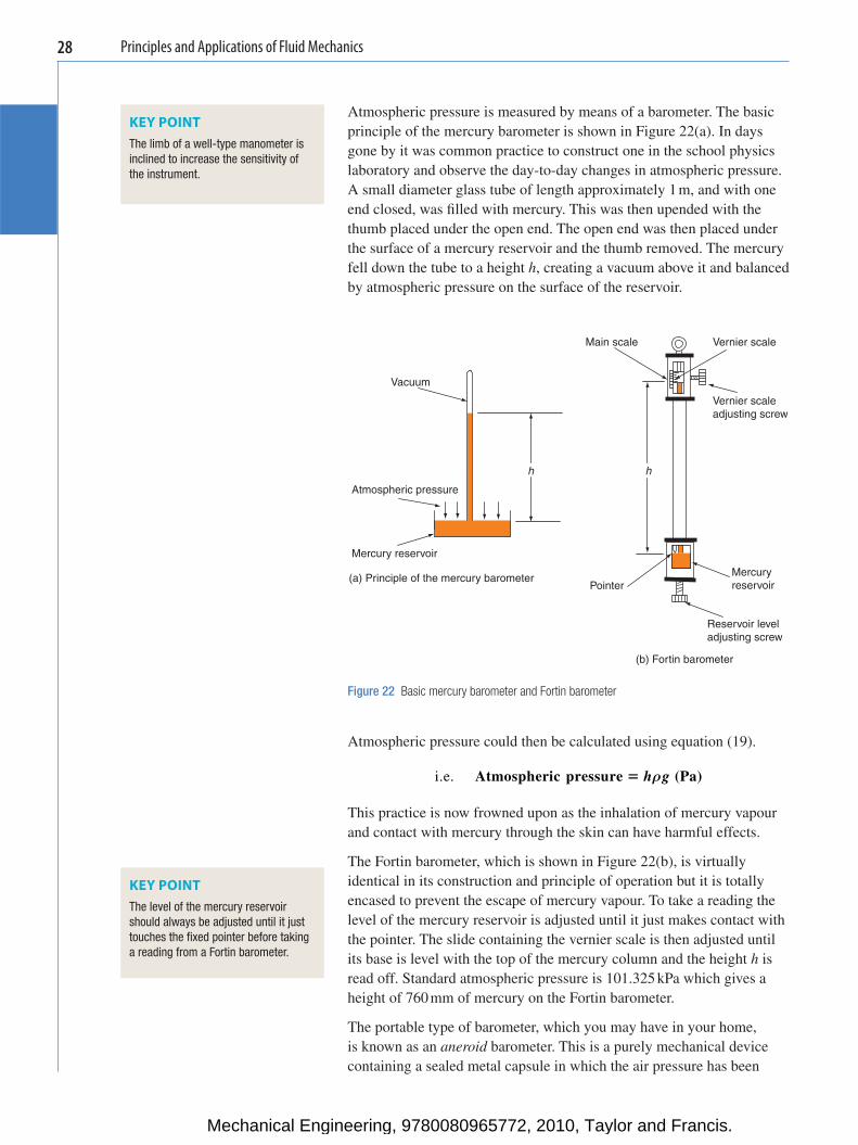
Atmospheric pressure is measured by means of a barometer. The basic principle of the mercury barometer is shown in Figure 22(a) . In days gone by it was common practice to construct one in the school physics laboratory and observe the day-to-day changes in atmospheric pressure. A small diameter glass tube of length approximately 1 m, and with one end closed, was fi lled with mercury. This was then upended with the thumb placed under the open end. The open end was then placed under the surface of a mercury reservoir and the thumb removed. The mercury fell down the tube to a height h , creating a vacuum above it and balanced by atmospheric pressure on the surface of the reservoir.
KEY POINT The limb of a well-type manometer is inclined to increase the sensitivity of the instrument.
Main scale Vernier scale
Vacuum
Vernier scale adjusting screw
h h
Atmospheric pressure
Mercury reservoir
Mercury reservoir
Reservoir level adjusting screw
Pointer(a) Principle of the mercury barometer
(b) Fortin barometer
Figure 22 Basic mercury barometer and Fortin barometer
Atmospheric pressure could then be calculated using equation (19).
i.e. Atmospheric pressure (Pa)� h gρ
This practice is now frowned upon as the inhalation of mercury vapour and contact with mercury through the skin can have harmful effects.
The Fortin barometer, which is shown in Figure 22(b) , is virtually identical in its construction and principle of operation but it is totally encased to prevent the escape of mercury vapour. To take a reading the level of the mercury reservoir is adjusted until it just makes contact with the pointer. The slide containing the vernier scale is then adjusted until its base is level with the top of the mercury column and the height h is read off. Standard atmospheric pressure is 101.325 kPa which gives a height of 760 mm of mercury on the Fortin barometer.
The portable type of barometer, which you may have in your home, is known as an aneroid barometer. This is a purely mechanical device containing a sealed metal capsule in which the air pressure has been
KEY POINT The level of the mercury reservoir should always be adjusted until it just touches the fi xed pointer before taking a reading from a Fortin barometer.
Mechanical Engineering, 9780080965772, 2010, Taylor and Francis.
Principles and Applications of Fluid Mechanics 29
reduced. Changes in atmospheric pressure cause the capsule to fl ex and the movement is amplifi ed through a mechanical linkage to move the pointer round the viewing scale. Although the display is usually calibrated to predict the weather conditions, it might also contain numbers around its periphery. These are the corresponding heights of a mercury column, given in either millimetres or inches.
Example 8 The gas pressure inside a container is measured by means of an inclined well-type manometer containing a fl uid of density 850 kg m � 3 . The angle of the inclined limb is 20° and the fl uid is observed to travel a distance of 410 mm along the inclined scale. A Fortin barometer shows that the prevailing atmospheric pressure corresponds to 755 mm Hg. What is the absolute pressure of the gas inside the container? The density of mercury is 13 600 kg m � 3 .
Finding the gauge pressure p g inside the container. Let the density of the oil in the inclined manometer be ρ 1 ·
p l g
p1 1
0 41 850�
� � �
sinsin g
θr
. 20�
pg 119 Pa�
Finding atmospheric pressure ρ a . Let the density of mercury be ρ 2 .
p h gp
a
a
�
� � �
ρ2
0 755 13600 9 81. .pa � 100 729 Pa
Finding absolute pressure p in the container.
p p p
p
� �
�
g a
119 + 100 729p � 100 848 Pa or 100.848 kPa
? Test your knowledge 3 1. How does the pressure below the free surface of a liquid vary with depth? 2. How does the thrust on the side of a rectangular section tank increase
with the depth of liquid contained? 3. Where is the centre of pressure on a vertical rectangular retaining surface? 4. What might an inclined well-type manometer, containing water, be used
for? 5. What is the procedure to be followed when taking a reading of
atmospheric pressure from a Fortin barometer?
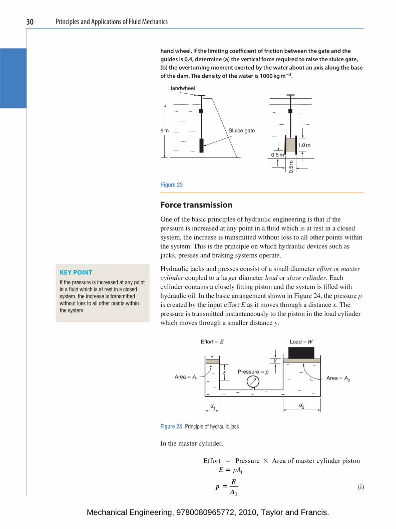
Activity 3 The rectangular wall of a dam is 20 m wide and contains a sluice gate of mass 50 kg as shown in Figure 23 . The gate can be raised in guides by means of the
Mechanical Engineering, 9780080965772, 2010, Taylor and Francis.
Principles and Applications of Fluid Mechanics30
hand wheel. If the limiting coeffi cient of friction between the gate and the guides is 0.4, determine (a) the vertical force required to raise the sluice gate, (b) the overturning moment exerted by the water about an axis along the base of the dam. The density of the water is 1000 kg m � 3 .
Force transmission
One of the basic principles of hydraulic engineering is that if the pressure is increased at any point in a fl uid which is at rest in a closed system, the increase is transmitted without loss to all other points within the system. This is the principle on which hydraulic devices such as jacks, presses and braking systems operate.
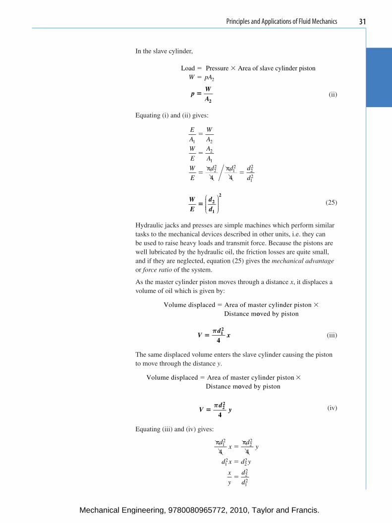
Hydraulic jacks and presses consist of a small diameter effort or master cylinder coupled to a larger diameter load or slave cylinder . Each cylinder contains a closely fi tting piston and the system is fi lled with hydraulic oil. In the basic arrangement shown in Figure 24 , the pressure p is created by the input effort E as it moves through a distance x . The pressure is transmitted instantaneously to the piston in the load cylinder which moves through a smaller distance y .
KEY POINT If the pressure is increased at any point in a fl uid which is at rest in a closed system, the increase is transmitted without loss to all other points within the system.
Effort � E Load �W
y x Pressure � p
Area � A1 Area � A2
d1d2
Figure 24 Principle of hydraulic jack
In the master cylinder,
Effort Pressure Area of master cylinder piston� �
E pA� 1
p
EA
�1
(i)
Handwheel
6 m Sluice gate
1.0 m
0.5 m
0.5
m
Figure 23
Mechanical Engineering, 9780080965772, 2010, Taylor and Francis.
Principles and Applications of Fluid Mechanics 31
In the slave cylinder,
Load Pressure Area of slave cylinder piston� �
�W pA2
p
WA
�2
(ii)
Equating (i) and (ii) gives:
E
A
W
A
W
E
A
A
W
E
d d d
d
1 2
2
1
22
12
22
124 4
�
�
� �� �
WE
d
d� 2
1
⎛
⎝⎜⎜⎜⎜
⎞
⎠⎟⎟⎟⎟
2
(25)
Hydraulic jacks and presses are simple machines which perform similar tasks to the mechanical devices described in other units, i.e. they can be used to raise heavy loads and transmit force. Because the pistons are well lubricated by the hydraulic oil, the friction losses are quite small, and if they are neglected, equation (25) gives the mechanical advantage or force ratio of the system.
As the master cylinder piston moves through a distance x , it displaces a volume of oil which is given by:
Volume displaced Area of master cylinder pistonDistance m
� �
ooved by piston
V
dx�
π 12
4 (iii)
The same displaced volume enters the slave cylinder causing the piston to move through the distance y .
Volume displaced Area of master cylinder pistonDistance m
� �
ooved by piston
V
dy�
π 22
4 (iv)
Equating (iii) and (iv) gives:
� �dx
dy
d x d y
x
y
d
d
12
22
12
22
22
4 4�
�
�12
Mechanical Engineering, 9780080965772, 2010, Taylor and Francis.
Principles and Applications of Fluid Mechanics32
xy
d
d� 2
1
⎛
⎝⎜⎜⎜⎜
⎞
⎠⎟⎟⎟⎟
2
(26)
This is the velocity ratio or movement ratio of the system, and as can be seen, it is equal to the mechanical advantage. It follows that when the effects of friction are small enough to be neglected, the two can be equated giving:
WE
xy
d
d� � 2
1
2⎛
⎝⎜⎜⎜⎜
⎞
⎠⎟⎟⎟⎟
(27)
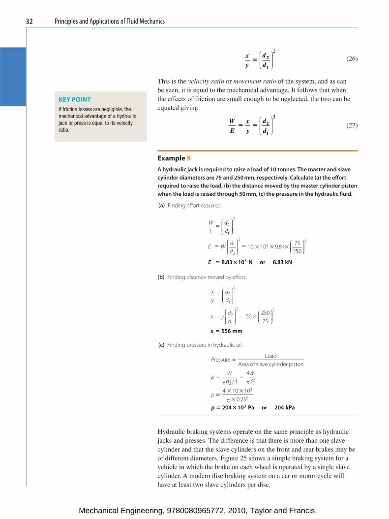
Example 9 A hydraulic jack is required to raise a load of 10 tonnes. The master and slave cylinder diameters are 75 and 250 mm, respectively. Calculate (a) the eff ort required to raise the load, (b) the distance moved by the master cylinder piston when the load is raised through 50 mm, (c) the pressure in the hydraulic fl uid.
(a) Finding eff ort required.
WE
E Wdd
�
� � � � �
d
d2
1
⎛
⎝⎜⎜⎜⎜
⎞
⎠⎟⎟⎟⎟⎟
⎛
⎝⎜⎜⎜⎜
⎞
⎠⎟⎟⎟⎟⎟
2
1
2
2
310 10 9 8175
2.
550
2⎛⎝⎜⎜⎜
⎞⎠⎟⎟⎟⎟
E � �8.83 10 N or 8.83 kN3
(b) Finding distance moved by eff ort.
xy
dd
x ydd
�
� � �
2
1
2
2
1
2
5025075
⎛
⎝⎜⎜⎜⎜
⎞
⎠⎟⎟⎟⎟⎟
⎛
⎝⎜⎜⎜⎜
⎞
⎠⎟⎟⎟⎟⎟
⎛⎝⎜⎜⎜
⎞⎠⎟⎟⎟⎟⎟
2
x � 556 mm
(c) Finding pressure in hydraulic oil.
P
pWd
Wd
p
ressure =Load
Area of slave cylinder piston
� �π π2
2224
4
��� �
�
4 10 100 25
3
2π .p � �204 10 Pa or 204 kPa3
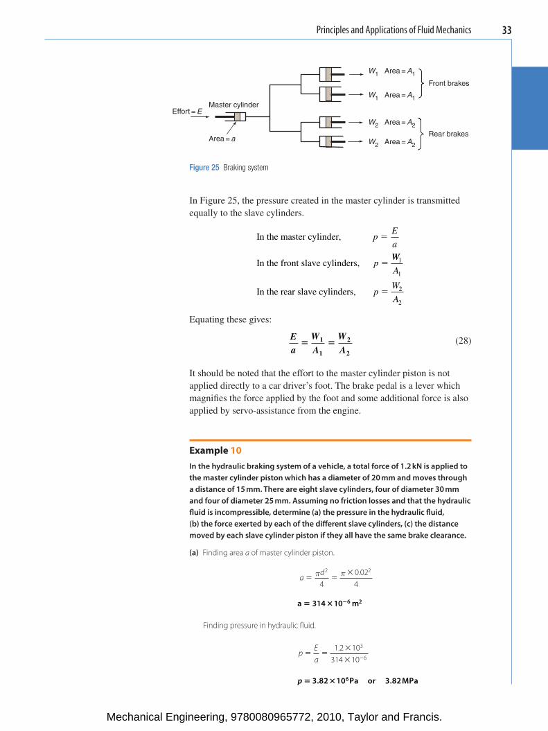
Hydraulic braking systems operate on the same principle as hydraulic jacks and presses. The difference is that there is more than one slave cylinder and that the slave cylinders on the front and rear brakes may be of different diameters. Figure 25 shows a simple braking system for a vehicle in which the brake on each wheel is operated by a single slave cylinder. A modern disc braking system on a car or motor cycle will have at least two slave cylinders per disc.
KEY POINT If friction losses are negligible, the mechanical advantage of a hydraulic jack or press is equal to its velocity ratio.
Mechanical Engineering, 9780080965772, 2010, Taylor and Francis.
Principles and Applications of Fluid Mechanics 33
In Figure 25 , the pressure created in the master cylinder is transmitted equally to the slave cylinders.
In the master cylinder,
In the front slave cylinders,
pE
a
p
�
�WW
A
pW
A
1
1
2
2
In the rear slave cylinders, �
Equating these gives:
Ea
W
A
W
A� �1
1
2
2
(28)
It should be noted that the effort to the master cylinder piston is not applied directly to a car driver’s foot. The brake pedal is a lever which magnifi es the force applied by the foot and some additional force is also applied by servo-assistance from the engine.
Example 10 In the hydraulic braking system of a vehicle, a total force of 1.2 kN is applied to the master cylinder piston which has a diameter of 20 mm and moves through a distance of 15 mm. There are eight slave cylinders, four of diameter 30 mm and four of diameter 25 mm. Assuming no friction losses and that the hydraulic fl uid is incompressible, determine (a) the pressure in the hydraulic fl uid, (b) the force exerted by each of the diff erent slave cylinders, (c) the distance moved by each slave cylinder piston if they all have the same brake clearance.
(a) Finding area a of master cylinder piston.
a
d� �
�π π2 2
40.024
a 314 10 m6 2� � �
Finding pressure in hydraulic fl uid.
p
Ea
� ��
� �
1.2 10314 10
3
6
p � �3.82 10 or 3.826Pa MPa
W1 Area = A1
W1 Area = A1
W2 Area = A2
W2 Area = A2
Front brakes
Master cylinderEffort = E
Rear brakesArea = a
Figure 25 Braking system
Mechanical Engineering, 9780080965772, 2010, Taylor and Francis.
Principles and Applications of Fluid Mechanics34
(b) Finding force W 1 exerted by the slave cylinder pistons whose diameter D 1 is 30 mm area is A 1 .
W pA pd
W
1 112
1
� �
� � ��
π
π4
3.82 100.034
62
W 2.7 10 N or 2.7kN13� �
Finding force W 2 exerted by the slave cylinder pistons whose diameter D 2 is 25 mm area is A 2 .
W pA pd
W
22
26
24
3.82 100.0254
� �
� � ��
2π
π
2
W 1.88 10 N or 1.88 kN23� �
(c) Finding distance y moved by slave cylinder pistons when master cylinder piston moves through a distance x � 15 mm.
Volume displaced in master cylinder = Total volume displaced iin slave cylinders
� � �dx
Dy
Dy
d x D y D y
d x
212
22
22
2
2
42
42
4
2
� �
� �2 12
�� �
��
��
�
2
2
0.02 0.0152(0.03 0.025 )
12
2
22
2
2
2 2
(
( )
D D y
yd x
D D
22
1
)
y
y � � �1.97 10 m or 1.973 mm
? Test your knowledge 4 1. How may the velocity ratio of a hydraulic jack be calculated from the
master and slave cylinder diameters? 2. What assumptions are made as to the compressibility of the hydraulic
fl uid when doing this calculation? 3. What assumption is made when the mechanical advantage and the
velocity ratio of a hydraulic jack are taken to be equal? 4. What is the essential difference between the hydraulic braking system
of a motor vehicle and basic hydraulic jack or press?
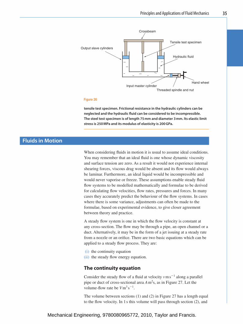
Activity 4 Figure 26 is a schematic diagram for a hydraulic tensile testing machine. Load is applied to the specimen by means of a hand wheel whose threaded spindle turns in a fi xed nut. The spindle moves the master cylinder piston whose diameter is 25 mm. The twin output slave cylinders are each 60 mm in diameter and are connected to a rigid crossbeam. This in turn transmits the load to the
Mechanical Engineering, 9780080965772, 2010, Taylor and Francis.
Principles and Applications of Fluid Mechanics 35
tensile test specimen. Frictional resistance in the hydraulic cylinders can be neglected and the hydraulic fl uid can be considered to be incompressible. The steel test specimen is of length 75 mm and diameter 3 mm. Its elastic limit stress is 250 MPa and its modulus of elasticity is 200 GPa.
Fluids in Motion
When considering fl uids in motion it is usual to assume ideal conditions. You may remember that an ideal fl uid is one whose dynamic viscosity and surface tension are zero. As a result it would not experience internal shearing forces, viscous drag would be absent and its fl ow would always be laminar. Furthermore, an ideal liquid would be incompressible and would never vaporise or freeze. These assumptions enable steady fl uid fl ow systems to be modelled mathematically and formulae to be derived for calculating fl ow velocities, fl ow rates, pressures and forces. In many cases they accurately predict the behaviour of the fl ow systems. In cases where there is some variance, adjustments can often be made to the formulae, based on experimental evidence, to give closer agreement between theory and practice.
A steady fl ow system is one in which the fl ow velocity is constant at any cross-section. The fl ow may be through a pipe, an open channel or a duct. Alternatively, it may be in the form of a jet issuing at a steady rate from a nozzle or an orifi ce. There are two basic equations which can be applied to a steady fl ow process. They are:
(i) the continuity equation (ii) the steady fl ow energy equation.
The continuity equation
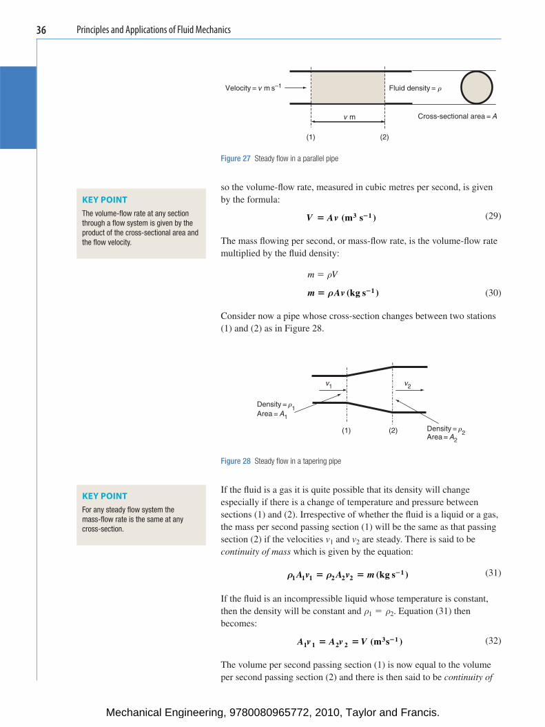
Consider the steady fl ow of a fl uid at velocity v m s � 1 along a parallel pipe or duct of cross-sectional area A m 2 s, as in Figure 27 . Let the volume-fl ow rate be V m 3 s � 1 .
The volume between sections (1) and (2) in Figure 27 has a length equal to the fl ow velocity. In 1 s this volume will pass through section (2), and
Crossbeam
Tensile test specimen
Output slave cylinders
Hydraulic fluid
Hand wheelInput master cylinder
Threaded spindle and nut
Figure 26
Mechanical Engineering, 9780080965772, 2010, Taylor and Francis.
Principles and Applications of Fluid Mechanics36
so the volume-fl ow rate, measured in cubic metres per second, is given by the formula:
V Av� �(m s )3 1
(29)
The mass fl owing per second, or mass-fl ow rate, is the volume-fl ow rate multiplied by the fl uid density:
m V� ρ
m Av� �ρ (kg s )1 (30)
Consider now a pipe whose cross-section changes between two stations (1) and (2) as in Figure 28 .
Velocity = v m s–1 Fluid density = r
v m Cross-sectional area = A
(1) (2)
Figure 27 Steady fl ow in a parallel pipe
KEY POINT The volume-fl ow rate at any section through a fl ow system is given by the product of the cross-sectional area and the fl ow velocity.
v1 v2
Density = r1
Area = A1
(1) (2) Density = r2
Area = A2
Figure 28 Steady fl ow in a tapering pipe
If the fl uid is a gas it is quite possible that its density will change especially if there is a change of temperature and pressure between sections (1) and (2). Irrespective of whether the fl uid is a liquid or a gas, the mass per second passing section (1) will be the same as that passing section (2) if the velocities v 1 and v 2 are steady. There is said to be continuity of mass which is given by the equation:
ρ ρ1 1 1 2 2 21(kg s )A v A v m� � �
(31)
If the fl uid is an incompressible liquid whose temperature is constant, then the density will be constant and ρ 1 � ρ 2 . Equation (31) then becomes:
A v A v V1 1 2 23 1(m s )� � �
(32)
The volume per second passing section (1) is now equal to the volume per second passing section (2) and there is then said to be continuity of
KEY POINT For any steady fl ow system the mass-fl ow rate is the same at any cross-section.
Mechanical Engineering, 9780080965772, 2010, Taylor and Francis.
Principles and Applications of Fluid Mechanics 37
volume . Substituting the expressions for cross-sectional area in place of A 1 and A 2 gives:
� �dv
d
d v d v
v
v
d
d
12
22
12
22
22
12
4 41 2
1 2
1
2
�
�
�
v
v
v
d
d1
2
2
1
2
�⎡
⎣⎢⎢
⎤
⎦⎥⎥
(33)
From this it will be seen that the ratio of the velocities at the two sections is equal to the inverse ratio of the diameters squared, i.e. if d 2 is twice the value of d 1 , then the velocity v 1 will be 4 times bigger than v 2 , etc.
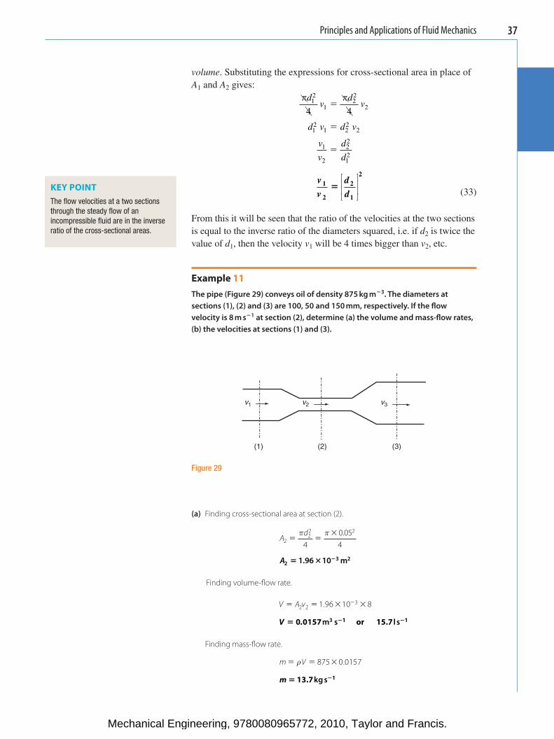
Example 11 The pipe ( Figure 29 ) conveys oil of density 875 kg m � 3 . The diameters at sections (1), (2) and (3) are 100, 50 and 150 mm, respectively. If the fl ow velocity is 8 m s � 1 at section (2), determine (a) the volume and mass-fl ow rates, (b) the velocities at sections (1) and (3).
KEY POINT The fl ow velocities at a two sections through the steady fl ow of an incompressible fl uid are in the inverse ratio of the cross-sectional areas.
v1 v2 v3
(3)(2)(1)
Figure 29
(a) Finding cross-sectional area at section (2).
A
d2
22
� ��π π
40.054
2
A23 21.96 10 m� � �
Finding volume-fl ow rate.
V A v� � � ��2 2
31.96 10 8
V .� � �0 0157 or 15.71 1m s l s3
Finding mass-fl ow rate.
m V� � �ρ 875 0.0157
m � �13.7 1kg s
Mechanical Engineering, 9780080965772, 2010, Taylor and Francis.
Principles and Applications of Fluid Mechanics38
(b) Finding velocity at section (1).
V A vd
v
vV
d
� �
� ��
�
1 112
1
2
π
π π
44 4 0.0157
0.1112
v112.0 m s� �
Finding velocity at section (3).
V A v
vVd
� �
� ��
�
3 33
2
3
332
4
π
π π
dv
4
4 0.01570.152
v .310 884� �m s
It will be noted that the velocity at section (2) is 4 times bigger than the velocity at section (1) and 9 times bigger than the velocity at section (3), as predicted by equation (33), i.e. the ratio of the velocities is equal to the inverse ratio of the
cross-sectional areas and of the diameters squared.
Energy of a fl uid
A moving fl uid can contain energy in a number of different forms. If the mass-fl ow rate is m kg s � 1 , the values of these energy forms, given as the energy per second passing a particular cross-section, are as follows.
(i) Gravitational potential energy : This is the work which has been done to raise the fl uid to its height, z m, measured above some given datum level.
Potential energy (J s W)1� �mgz or (34)
(ii) Kinetic energy : This is the work which has been done in accelerating the fl uid from rest up to some particular velocity v m s � 1 .
Kinetic energy
12
(J s W)2 1� �mv or
(35)
(iii) Internal energy : This is the energy contained in a fl uid by virtue of the absolute temperature, T K, to which it has been raised. It is the sum of the individual kinetic energies of the molecules of the fl uid. These are in a state of random motion and their kinetic energy is directly proportional to the absolute temperature of the fl uid. It is separate from the above linear kinetic energy of fl ow. A fl uid at a particular temperature has the same internal energy when stationary and when it is in motion. It is diffi cult to calculate internal energy although the changes of internal energy which accompany temperature change can be determined and will be considered in
Mechanical Engineering, 9780080965772, 2010, Taylor and Francis.
Principles and Applications of Fluid Mechanics 39
the Principles and Applications of Thermodynamics unit. Internal energy is generally expressed as:
Internal energy (J s W)1� �U or (36)
(iv) Pressure-fl ow energy : This is also called fl ow work and work of introduction . It is the energy of the fl uid by virtue of its pressure, p Pa. This is the pressure to which it has been raised by a pump, fan or compressor to make it fl ow into or through a system against the prevailing back-pressure. It is analogous to the work that must be done against friction to keep a solid body in motion.
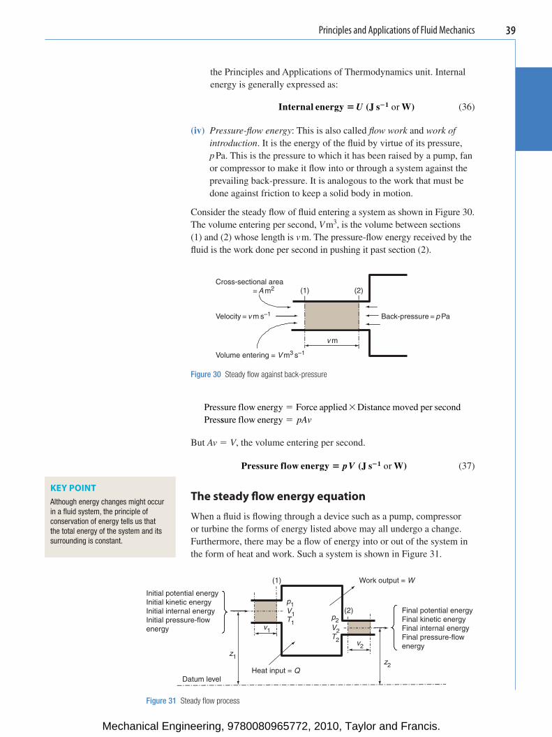
Consider the steady fl ow of fl uid entering a system as shown in Figure 30 . The volume entering per second, V m 3 , is the volume between sections (1) and (2) whose length is v m. The pressure-fl ow energy received by the fl uid is the work done per second in pushing it past section (2).
Cross-sectional area = A m2 (1) (2)
Velocity = v m s–1 Back-pressure = p Pa
v m
Volume entering = V m3 s–1
Figure 30 Steady fl ow against back-pressure
Pressure flow energy Force applied Distance moved per secondPres
� �
ssure flow energy � pAv
But Av � V , the volume entering per second.
Pressure flow energy (J s W)1� �pV or (37)
The steady fl ow energy equation
When a fl uid is fl owing through a device such as a pump, compressor or turbine the forms of energy listed above may all undergo a change. Furthermore, there may be a fl ow of energy into or out of the system in the form of heat and work. Such a system is shown in Figure 31 .
KEY POINT Although energy changes might occur in a fl uid system, the principle of conservation of energy tells us that the total energy of the system and its surrounding is constant.
(1) Work output = W
Initial potential energyInitial kinetic energyInitial internal energyInitial pressure-flow energy
p1V1 (2) Final potential energy
Final kinetic energyFinal internal energyFinal pressure-flow energy
T1p2
v1 V2 T2
v2 z1
z2Heat input = Q
Datum level
Figure 31 Steady fl ow process
Mechanical Engineering, 9780080965772, 2010, Taylor and Francis.
Principles and Applications of Fluid Mechanics40
For steady fl ow conditions, the mass per second fl owing into the system is equal to the mass per second leaving. Also the energy per second entering the system must equal the energy per second leaving. It follows that for the system shown in Figure 31 ,
Initial potential energy + Initial kinetic energy +Initial internall energy + Initial pressure flow energy +Heat energy input = Final pottential energy + Final kinetic energy +Final internal energy + Finall pressure flow energy +Work output
Substituting the expressions which have been derived for these terms gives:
mgz mv U p V Q mgz mv U p V W1 1
21 1 1 2 2
22 2 2
12
12
� � � � � � � � �
(38)
This is known as the full steady fl ow energy equation (FSFEE) which we shall make use of in Chapter 6 in the study of thermodynamics. It is also very useful in the study of fl uid mechanics but here we change it into a more usable form which is known as Bernoulli’s equation .
Bernoulli’s equation
In the study of liquids fl owing steadily through a pipe or channel, or issuing from a nozzle in the form of a jet, it is assumed that temperature changes are so small as to be negligible. This means that there is little or no change in internal energy, i.e. U 1 � U 2 , and that these terms can be eliminated from the steady fl ow energy equation. It is also assumed that no heat transfer takes place and that no external work is done, i.e. Q � 0 and W � 0, and these terms can also be eliminated. The steady fl ow energy equation thus reduces to:
mgz mv p V mgz mv p V1 1 1 2 2 2
1
2
1
2� � � � �1
222
Dividing throughout by the product mg gives:
z
v
g
p V
mgz
v
g
p V
mg11 1
22 2
2 2� � � � �1
222
Now for an incompressible liquid, V
m
V
m1 2� �
1
ρ where ρ is the density
of the liquid.
Substituting and rearranging gives:
p
g
v
gz
p
g
v
gz1 1
2
12 2
2
22 2ρ ρ� � � �
(39)
Mechanical Engineering, 9780080965772, 2010, Taylor and Francis.
Principles and Applications of Fluid Mechanics 41
This is Bernoulli’s equation in which the units of each term are metres. Dividing throughout by mg has changed the units from joules per second or watts to the equivalent potential energy height, or head , measured in metres.
The terms are called .
The terms are ca
pg
vg
ρpressure heads
2
2llled .
The terms are called
velocity heads
potential headsz .
The terms on each side of Bernoulli’s equation give the total head at section (1) of a steady fl ow system which is equal to the total head at section (2). In practice there is often some energy loss z f due to viscous resistance and turbulence, particularly on long pipelines. This can sometimes be estimated and added to the right-hand side of Bernoulli’s equation to give:
p
g
v
gz
p
g
v
gz z1 1
2
12 2
2
2 f2 2ρ ρ� � � � � �
(40)
When used together, the continuity equation (32) and Bernoulli’s equation (40) can solve many problems concerned with steady fl ow. Sometimes they have to be solved as simultaneous equations as in Example 12. This provides an opportunity for you to put into practice some of the mathematical techniques which you have learned.
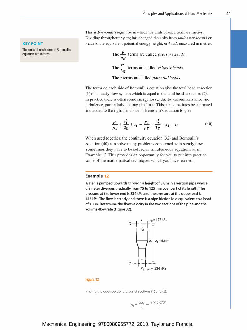
Example 12 Water is pumped upwards through a height of 8.8 m in a vertical pipe whose diameter diverges gradually from 75 to 125 mm over part of its length. The pressure at the lower end is 234 kPa and the pressure at the upper end is 145 kPa. The fl ow is steady and there is a pipe friction loss equivalent to a head of 1.2 m. Determine the fl ow velocity in the two sections of the pipe and the volume-fl ow rate ( Figure 32 ).
KEY POINT The units of each term in Bernoulli’s equation are metres.
p2 = 175 kPa(2)
v2
z2 – z1 = 8.8 m
(1)v1
p1 = 234 kPa
Figure 32
Finding the cross-sectional areas at sections (1) and (2).
A
d1
2
40.0754
� ��π π1
2
Mechanical Engineering, 9780080965772, 2010, Taylor and Francis.
Principles and Applications of Fluid Mechanics42
A13 24.42 10� � � m
A
d2
2
50.1254
� ��π π2
2
A23 212.27 10� � � m
Applying continuity equation to sections (1) and (2)
A v A v
vAA
v v
1 1 2 2
12
12
3
3 212.27 10
�
� ��
��
�
�4 42 10.
v v1 22.78� (i)
Applying Bernoulli’s equation to sections (1) and (2):
pg
vg
zp
gv
gz z
vg
vg
pg
pg
z z
11
2
2 1
2 2
2 2
ρ ρ
ρ ρ
� � � � � �
� � � � � �
12
22
2
12
22
2 1
f
zz
v v gp p
gz z z
v v
f
f12
22 2 1
2 1
12
22
� ��
� � �
� � ��
2
2 9 81(145 23
ρ
⎡
⎣⎢⎢
⎤
⎦⎥⎥
.44) 10
1000 9.818 8 1 2
3�
�� �. .
⎡
⎣⎢⎢
⎤
⎦⎥⎥
v v12
22 18.2� �
(ii)
Substitute for v 1 from (i)
2 78 18.2
(2.78 1) 18.2
1 78 18 2
18.21.78
.
. .
v v
v
v
v
22
22
22
22
2
� �
� �
�
�
v213 2� �. m s
Finding v 1 from (i)
v v1 22.78 2.78 3.2� � �
v118 9� �. m s
Finding volume-fl ow rate.
V A V� � � ��2 2 12 27 10 3.23.
V � � � � �39.3 10 or 39 33 1m s l s3 1.
Mechanical Engineering, 9780080965772, 2010, Taylor and Francis.
Principles and Applications of Fluid Mechanics 43
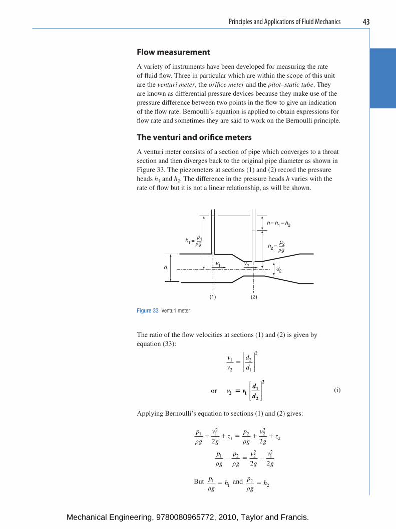
Flow measurement
A variety of instruments have been developed for measuring the rate of fl uid fl ow. Three in particular which are within the scope of this unit are the venturi meter , the orifi ce meter and the pitot–static tube . They are known as differential pressure devices because they make use of the pressure difference between two points in the fl ow to give an indication of the fl ow rate. Bernoulli’s equation is applied to obtain expressions for fl ow rate and sometimes they are said to work on the Bernoulli principle.
The venturi and orifi ce meters
A venturi meter consists of a section of pipe which converges to a throat section and then diverges back to the original pipe diameter as shown in Figure 33 . The piezometers at sections (1) and (2) record the pressure heads h 1 and h 2 . The difference in the pressure heads h varies with the rate of fl ow but it is not a linear relationship, as will be shown.
h = h1 – h2
h1 = p2rg
d1
v1 v2 d2
(1)
rg
(2)
h2 =
p1
Figure 33 Venturi meter
The ratio of the fl ow velocities at sections (1) and (2) is given by equation (33):
v
v
d
d1
2
� 2
1
2⎡
⎣⎢⎢
⎤
⎦⎥⎥
or v v
d
d2 11
2
2
�⎡
⎣⎢⎢
⎤
⎦⎥⎥
(i)
Applying Bernoulli’s equation to sections (1) and (2) gives:
p
g
v
gz
p
g
v
gz
p
g
p
g
v
g
v
g
1 22
1 2
2 2
2 2
ρ ρ
ρ ρ
� � � � �
� � �
12
122
22
12
But
p
gh1
1ρ�
and p
gh2
2ρ�
Mechanical Engineering, 9780080965772, 2010, Taylor and Francis.
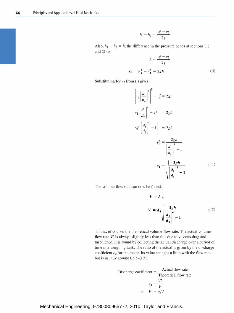
Principles and Applications of Fluid Mechanics44
h h
v v
g1 222
12
2� �
�
Also, h 1 � h 2 � h , the difference in the pressure heads at sections (1) and (2) is:
h
v v
g�
�22
12
2
or v v gh22
12 2� �
(ii)
Substituting for v 2 from (i) gives:
vd
dv gh
vd
dv gh
11
2
2 2
4
2
2
⎡
⎣⎢⎢
⎤
⎦⎥⎥
⎡
⎣
⎢⎢⎢
⎤
⎦
⎥⎥⎥
⎡
⎣⎢⎢
⎤
⎦⎥⎥
� �
� �
12
12
121
2
vvd
dgh
vgh
d
d
12
12
4
1
2
4
1
2
1 2
2
1
⎡
⎣⎢⎢
⎤
⎦⎥⎥
⎡
⎣
⎢⎢⎢
⎤
⎦
⎥⎥⎥
⎡
⎣⎢⎢
⎤
⎦⎥⎥
� �
�
�
vgh
dd
1
1
2
4
2
1
�
�⎡
⎣⎢⎢
⎤
⎦⎥⎥
(41)
The volume-fl ow rate can now be found.
V A v� 1 1
V Agh
dd
�
�
1
1
2
4
2
1⎡
⎣⎢⎢
⎤
⎦⎥⎥
(42)
This is, of course, the theoretical volume-fl ow rate. The actual volume-fl ow rate V � is always slightly less than this due to viscous drag and turbulence. It is found by collecting the actual discharge over a period of time in a weighing tank. The ratio of the actual is given by the discharge coeffi cient c d for the meter. Its value changes a little with the fl ow rate but is usually around 0.95–0.97.
Discharge coefficientActual flow rate
Theoretical flow rate
d
�
�cV��
� �
VV c Vor d
Mechanical Engineering, 9780080965772, 2010, Taylor and Francis.
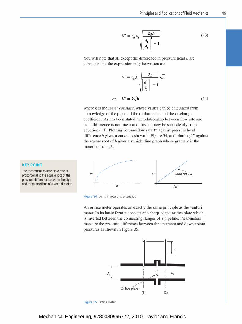
Principles and Applications of Fluid Mechanics 45
V cgh
dd
d� �
�
A1
1
2
4
2
1⎡
⎣⎢⎢
⎤
⎦⎥⎥
(43)
You will note that all except the difference in pressure head h are constants and the expression may be written as:
V cg
d
d
� �
�
d A h1
1
2
4
2
1⎡
⎣⎢⎢
⎤
⎦⎥⎥
or V k h� � (44)
where k is the meter constant , whose values can be calculated from a knowledge of the pipe and throat diameters and the discharge coeffi cient. As has been stated, the relationship between fl ow rate and head difference is not linear and this can now be seen clearly from equation (44). Plotting volume-fl ow rate V � against pressure head difference h gives a curve, as shown in Figure 34 , and plotting V � against the square root of h gives a straight line graph whose gradient is the meter constant, k .
KEY POINT The theoretical volume-fl ow rate is proportional to the square root of the pressure difference between the pipe and throat sections of a venturi meter.
V ′ V ′ Gradient = k
h h
Figure 34 Venturi meter characteristics
h
d1d2
Orifice plate(1) (2)
Figure 35 Orifi ce meter
An orifi ce meter operates on exactly the same principle as the venturi meter. In its basic form it consists of a sharp-edged orifi ce plate which is inserted between the connecting fl anges of a pipeline. Piezometers measure the pressure difference between the upstream and downstream pressures as shown in Figure 35 .
Mechanical Engineering, 9780080965772, 2010, Taylor and Francis.
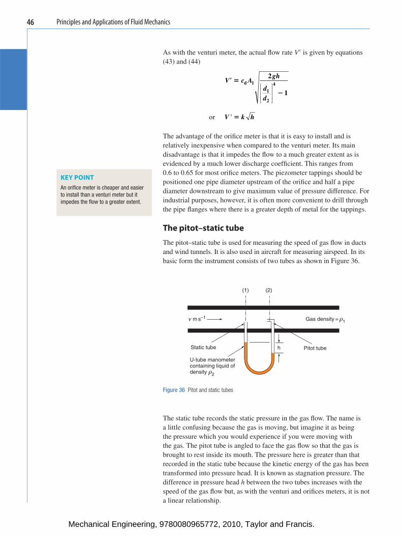
Principles and Applications of Fluid Mechanics46
As with the venturi meter, the actual fl ow rate V � is given by equations (43) and (44)
V c Agh
dd
� �
�
d 1 4
2
11
2
⎡
⎣⎢⎢
⎤
⎦⎥⎥
or V k h� �
The advantage of the orifi ce meter is that it is easy to install and is relatively inexpensive when compared to the venturi meter. Its main disadvantage is that it impedes the fl ow to a much greater extent as is evidenced by a much lower discharge coeffi cient. This ranges from 0.6 to 0.65 for most orifi ce meters. The piezometer tappings should be positioned one pipe diameter upstream of the orifi ce and half a pipe diameter downstream to give maximum value of pressure difference. For industrial purposes, however, it is often more convenient to drill through the pipe fl anges where there is a greater depth of metal for the tappings.
The pitot–static tube
The pitot–static tube is used for measuring the speed of gas fl ow in ducts and wind tunnels. It is also used in aircraft for measuring airspeed. In its basic form the instrument consists of two tubes as shown in Figure 36 .
KEY POINT An orifi ce meter is cheaper and easier to install than a venturi meter but it impedes the fl ow to a greater extent.
(1) (2)
v m s–1 Gas density = r1
Static tube h Pitot tube
U-tube manometercontaining liquid ofdensity r2
Figure 36 Pitot and static tubes
The static tube records the static pressure in the gas fl ow. The name is a little confusing because the gas is moving, but imagine it as being the pressure which you would experience if you were moving with the gas. The pitot tube is angled to face the gas fl ow so that the gas is brought to rest inside its mouth. The pressure here is greater than that recorded in the static tube because the kinetic energy of the gas has been transformed into pressure head. It is known as stagnation pressure. The difference in pressure head h between the two tubes increases with the speed of the gas fl ow but, as with the venturi and orifi ces meters, it is not a linear relationship.
Mechanical Engineering, 9780080965772, 2010, Taylor and Francis.
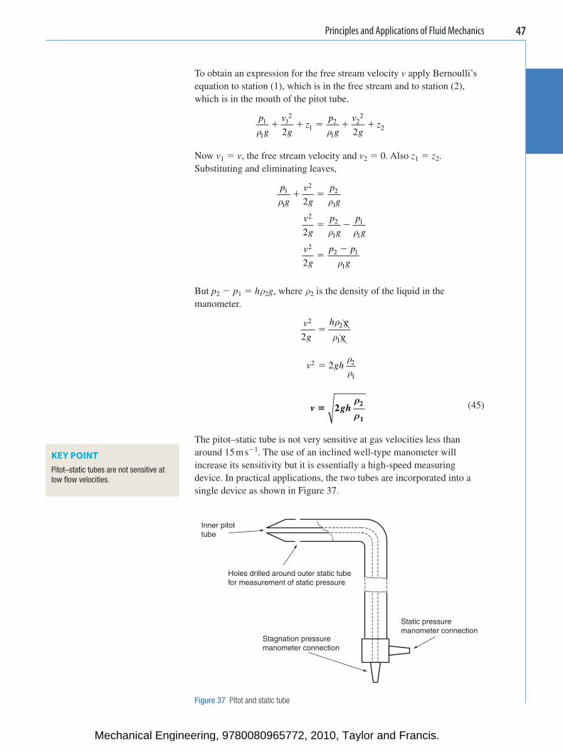
Principles and Applications of Fluid Mechanics 47
To obtain an expression for the free stream velocity v apply Bernoulli’s equation to station (1), which is in the free stream and to station (2), which is in the mouth of the pitot tube.
p
g
v
gz
p
g
v
gz1
1ρ ρ� � � � �1
2
12
1
22
22 2
Now v 1 � v , the free stream velocity and v 2 � 0. Also z 1 � z 2 . Substituting and eliminating leaves,
p
g
v
g
p
g
v
g
p
g
p
g
v
g
p p
g
1
1
22
1
22
1
1
1
22 1
1
2
2
2
ρ ρ
ρ ρ
ρ
� �
� �
��
But p 2 � p 1 � h ρ 2 g , where ρ 2 is the density of the liquid in the manometer.
v
g
h g
g
22
12 �
ρ
ρ
v gh2 2
1
2�ρρ
v gh� 2 2
1
ρ
ρ
(45)
The pitot–static tube is not very sensitive at gas velocities less than around 15 m s � 1 . The use of an inclined well-type manometer will increase its sensitivity but it is essentially a high-speed measuring device. In practical applications, the two tubes are incorporated into a single device as shown in Figure 37 .
KEY POINT Pitot–static tubes are not sensitive at low fl ow velocities.
Inner pitottube
Holes drilled around outer static tubefor measurement of static pressure
Static pressuremanometer connection
Stagnation pressuremanometer connection
Figure 37 Pitot and static tube
Mechanical Engineering, 9780080965772, 2010, Taylor and Francis.
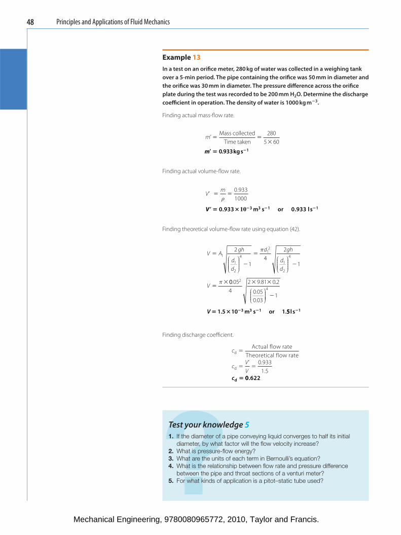
Principles and Applications of Fluid Mechanics48
Example 13 In a test on an orifi ce meter, 280 kg of water was collected in a weighing tank over a 5-min period. The pipe containing the orifi ce was 50 mm in diameter and the orifi ce was 30 mm in diameter. The pressure diff erence across the orifi ce plate during the test was recorded to be 200 mm H 2 O. Determine the discharge coeffi cient in operation. The density of water is 1000 kg m� 3 .
Finding actual mass-fl ow rate.
m’Mass collected
Time taken� �
�
2805 60
m� � �0 933kg s 1.
Finding actual volume-fl ow rate.
Vm
’
� �ρ
0.9331000
V’ � � � � �0.933 m s or 0.933 l s3 3 1 110
Finding theoretical volume-fl ow rate using equation (42).
V Agh
dd
d gh
dd
V
�
�
�
�
��
1
1
2
412
1
2
4
2
14
2
1⎛
⎝⎜⎜⎜⎜
⎞
⎠⎟⎟⎟⎟
⎛
⎝⎜⎜⎜⎜
⎞
⎠⎟⎟⎟⎟
π
π 00 054
2 9 81 0 2
0 050 03
1
2
4
. .
.
.
� �
�
.
⎛⎝⎜⎜⎜
⎞⎠⎟⎟⎟⎟
V � � � �1.5 10 m s or 1.3 3 1 55l s 1�
Finding discharge coeffi cient.
c
cVV
d
d
Actual flow rateTheoretical flow rate’
�
� �0 933
1 5.
.cd � 00.622
? Test your knowledge 5 1. If the diameter of a pipe conveying liquid converges to half its initial
diameter, by what factor will the fl ow velocity increase? 2. What is pressure-fl ow energy? 3. What are the units of each term in Bernoulli’s equation? 4. What is the relationship between fl ow rate and pressure difference
between the pipe and throat sections of a venturi meter? 5. For what kinds of application is a pitot–static tube used?
Mechanical Engineering, 9780080965772, 2010, Taylor and Francis.
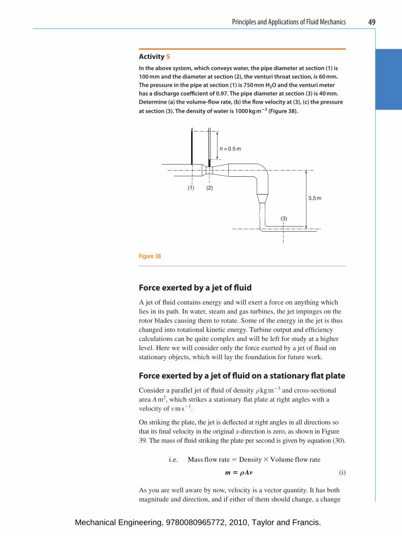
Principles and Applications of Fluid Mechanics 49
Activity 5 In the above system, which conveys water, the pipe diameter at section (1) is 100 mm and the diameter at section (2), the venturi throat section, is 60 mm. The pressure in the pipe at section (1) is 750 mm H 2 O and the venturi meter has a discharge coeffi cient of 0.97. The pipe diameter at section (3) is 40 mm. Determine (a) the volume-fl ow rate, (b) the fl ow velocity at (3), (c) the pressure at section (3). The density of water is 1000 kg m � 3 ( Figure 38 ).
Force exerted by a jet of fl uid
A jet of fl uid contains energy and will exert a force on anything which lies in its path. In water, steam and gas turbines, the jet impinges on the rotor blades causing them to rotate. Some of the energy in the jet is thus changed into rotational kinetic energy. Turbine output and effi ciency calculations can be quite complex and will be left for study at a higher level. Here we will consider only the force exerted by a jet of fl uid on stationary objects, which will lay the foundation for future work.
Force exerted by a jet of fl uid on a stationary fl at plate
Consider a parallel jet of fl uid of density ρ kg m � 3 and cross-sectional area A m 2 , which strikes a stationary fl at plate at right angles with a velocity of v m s � 1 .
On striking the plate, the jet is defl ected at right angles in all directions so that its fi nal velocity in the original x -direction is zero, as shown in Figure 39 . The mass of fl uid striking the plate per second is given by equation (30).
i.e. Mass flow rate Density Volume flow rate� �
m Av� ρ
(i)
As you are well aware by now, velocity is a vector quantity. It has both magnitude and direction, and if either of them should change, a change
h = 0.5 m
(1) (2)
3.5 m
(3)
Figure 38
Mechanical Engineering, 9780080965772, 2010, Taylor and Francis.
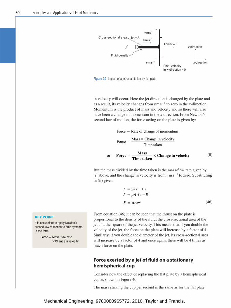
Principles and Applications of Fluid Mechanics50
in velocity will occur. Here the jet direction is changed by the plate and as a result, its velocity changes from v m s � 1 to zero in the x -direction. Momentum is the product of mass and velocity and so there will also have been a change in momentum in the x -direction. From Newton’s second law of motion, the force acting on the plate is given by:
Force Rate of change of momentum
ForceMass Change in velocity
Tim
�
��
ee taken
or Force
MassTime taken
Change in velocity� �
(ii)
But the mass divided by the time taken is the mass-fl ow rate given by (i) above, and the change in velocity is from v m s � 1 to zero. Substituting in (ii) gives:
F m vF Av v
� �
� �
( )( )
00ρ
F Av� ρ 2
(46)
From equation (46) it can be seen that the thrust on the plate is proportional to the density of the fl uid, the cross-sectional area of the jet and the square of the jet velocity. This means that if you double the velocity of the jet, the force on the plate will increase by a factor of 4. Similarly, if you double the diameter of the jet, its cross-sectional area will increase by a factor of 4 and once again, there will be 4 times as much force on the plate.
Force exerted by a jet of fl uid on a stationary hemispherical cup
Consider now the effect of replacing the fl at plate by a hemispherical cup as shown in Figure 40 .
The mass striking the cup per second is the same as for the fl at plate.
v m s–1
Cross-sectional area of jet = Av m s–1
Thrust = Fy-direction
Fluid density = r
v m s–1 x-directionFinal velocity in x-direction = 0
Figure 39 Impact of a jet on a stationary fl at plate
KEY POINTIt is convenient to apply Newton’s second law of motion to fl uid systems in the form
Force Mass-flow rateChange in velocity
��
Mechanical Engineering, 9780080965772, 2010, Taylor and Francis.
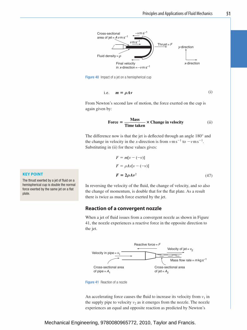
Principles and Applications of Fluid Mechanics 51
i.e. m Av� ρ (i)
From Newton’s second law of motion, the force exerted on the cup is again given by:
Force
MassTime taken
Change in velocity� �
(ii)
The difference now is that the jet is defl ected through an angle 180 ° and the change in velocity in the x -direction is from v m s � 1 to � v m s � 1 . Substituting in (ii) for these values gives:
F m v v
F Av v v
� � �
� � �
[ ]
[ ]
( )
( )ρ
F Av� 2ρ 2 (47)
In reversing the velocity of the fl uid, the change of velocity, and so also the change of momentum, is double that for the fl at plate. As a result there is twice as much force exerted by the jet.
Reaction of a convergent nozzle
When a jet of fl uid issues from a convergent nozzle as shown in Figure 41 , the nozzle experiences a reactive force in the opposite direction to the jet.
–v m s–1Cross-sectionalarea of jet = A v m s–1
Thrust = Fy-direction
Fluid density = r
Final velocityin x-direction = –v m s–1
x-direction
v m s–1
Figure 40 Impact of a jet on a hemispherical cup
KEY POINT The thrust exerted by a jet of fl uid on a hemispherical cup is double the normal force exerted by the same jet on a fl at plate.
Reactive force = FVelocity of jet = v2
Velocity in pipe = v1
Mass flow rate = m kg s–1
Cross-sectional areaof pipe = A1
Cross-sectional areaof jet = A2
Figure 41 Reaction of a nozzle
An accelerating force causes the fl uid to increase its velocity from v 1 in the supply pipe to velocity v 2 as it emerges from the nozzle. The nozzle experiences an equal and opposite reaction as predicted by Newton’s
Mechanical Engineering, 9780080965772, 2010, Taylor and Francis.
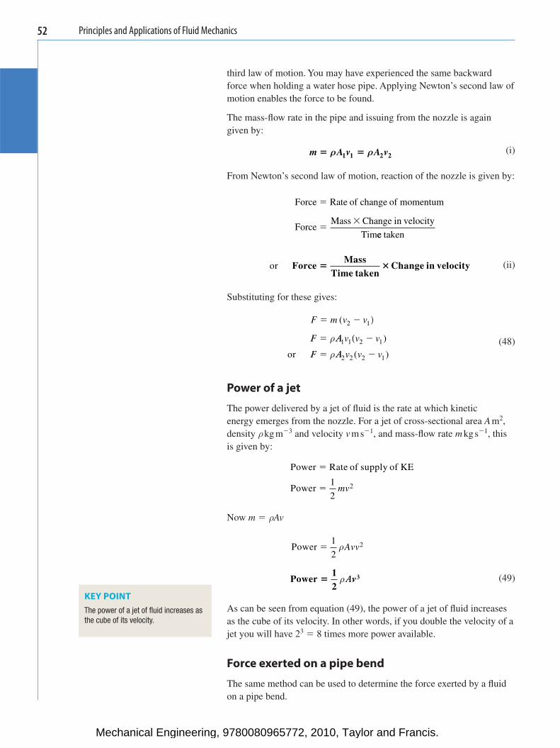
Principles and Applications of Fluid Mechanics52
third law of motion. You may have experienced the same backward force when holding a water hose pipe. Applying Newton’s second law of motion enables the force to be found.
The mass-fl ow rate in the pipe and issuing from the nozzle is again given by:
m A v A v� �ρ ρ1 1 2 2 (i)
From Newton’s second law of motion, reaction of the nozzle is given by:
Force Rate of change of momentum
ForceMass Change in velocity
Tim
�
��
ee taken
or Force
MassTime taken
Change in velocity� �
(ii)
Substituting for these gives:
F m v v� �( 2 1 )
F A
F A
� �
� �
ρ
ρ1 1 2 1
2 2 2 1
v v v
v v v
( )
( )or
(48)
Power of a jet
The power delivered by a jet of fl uid is the rate at which kinetic energy emerges from the nozzle. For a jet of cross-sectional area A m 2 , density ρ kg m � 3 and velocity v m s � 1 , and mass-fl ow rate m kg s � 1 , this is given by:
Power Rate of supply of KE
Power1
2
�
� mv2
Now m � ρ Av
Power �
1
22ρAvv
Power
12
� ρAv3
(49)
As can be seen from equation (49), the power of a jet of fl uid increases as the cube of its velocity. In other words, if you double the velocity of a jet you will have 2 3 � 8 times more power available.
Force exerted on a pipe bend
The same method can be used to determine the force exerted by a fl uid on a pipe bend.
KEY POINT The power of a jet of fl uid increases as the cube of its velocity.
Mechanical Engineering, 9780080965772, 2010, Taylor and Francis.
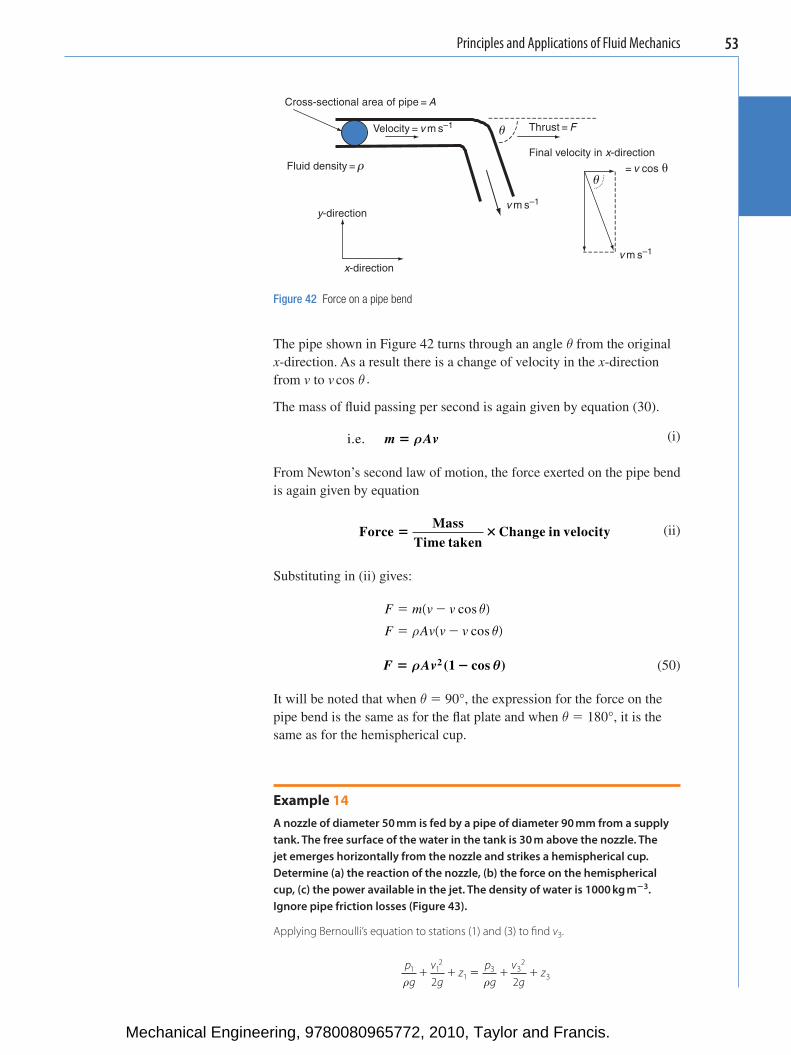
Principles and Applications of Fluid Mechanics 53
The pipe shown in Figure 42 turns through an angle θ from the original x -direction. As a result there is a change of velocity in the x -direction from v to v cos θ ·
The mass of fl uid passing per second is again given by equation (30).
i.e. m Av� ρ (i)
From Newton’s second law of motion, the force exerted on the pipe bend is again given by equation
Force
MassTime taken
Change in velocity� �
(ii)
Substituting in (ii) gives:
F m v v
F Av v v
� �
� �
( )
( )
cos
cos
θ
ρ θ
F Av� �ρ θ2 (1 cos ) (50)
It will be noted that when θ � 90°, the expression for the force on the pipe bend is the same as for the fl at plate and when θ � 180°, it is the same as for the hemispherical cup.
Example 14 A nozzle of diameter 50 mm is fed by a pipe of diameter 90 mm from a supply tank. The free surface of the water in the tank is 30 m above the nozzle. The jet emerges horizontally from the nozzle and strikes a hemispherical cup. Determine (a) the reaction of the nozzle, (b) the force on the hemispherical cup, (c) the power available in the jet. The density of water is 1000 kg m � 3 . Ignore pipe friction losses ( Figure 43 ).
Applying Bernoulli’s equation to stations (1) and (3) to fi nd v 3 .
pg
vg
zp
gv
gz1 1
2
13 3
2
32 2ρ ρ� � � ��
Cross-sectional area of pipe = A
Velocity = v m s–1 Thrust = F
Final velocity in x-direction
= v cos �Fluid density = r
v m s–1y-direction
v m s–1
x-direction
u
u
Figure 42 Force on a pipe bend
Mechanical Engineering, 9780080965772, 2010, Taylor and Francis.
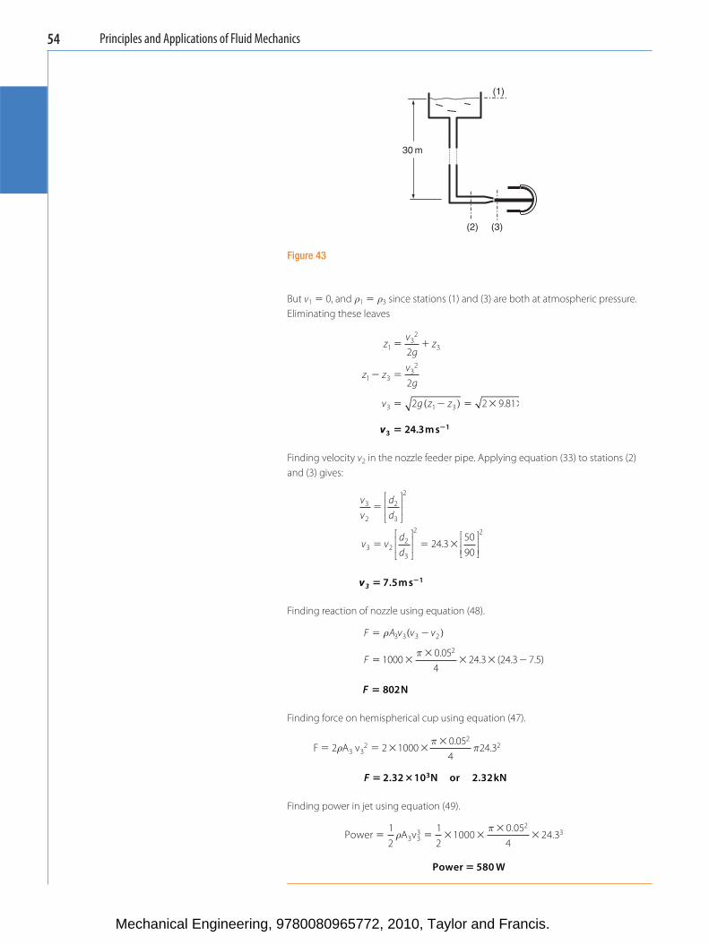
Principles and Applications of Fluid Mechanics54
But v 1 � 0, and ρ 1 � ρ 3 since stations (1) and (3) are both at atmospheric pressure. Eliminating these leaves
zv
gz
z zv
g
v g z z
13
2
3
1 33
2
3 1 3
2
2 2
� �
� �
� � � � �
2
9.81( )
v3124.3m s� �
Finding velocity v 2 in the nozzle feeder pipe. Applying equation (33) to stations (2) and (3) gives:
vv
dd
v vdd
3
2
2
3
2
3 22
3
2
�
� � �
⎡
⎣⎢⎢
⎤
⎦⎥⎥
⎡
⎣⎢⎢
⎤
⎦⎥⎥
⎡
⎣⎢⎢
⎤
⎦⎥⎥
24.35090
2
v3 � �7 5 1. m s
Finding reaction of nozzle using equation (48).
F A v v v
F
� �
� ��
� � �
ρ
π
3 3 3 2( )
10000.054
24.3 (24.3 7.5)2
F � 802N
Finding force on hemispherical cup using equation (47).
F 2 A v 2 1000
0.054
24.33 32
22� � � �
�ρ
ππ
F � �2 32 10 2 323. .N kNor
Finding power in jet using equation (49).
Power
12
A v12
10000.054
24.33 33
23� � � �
��ρ
π
Power W� 580
(1)
30 m
(2) (3)
Figure 43
Mechanical Engineering, 9780080965772, 2010, Taylor and Francis.
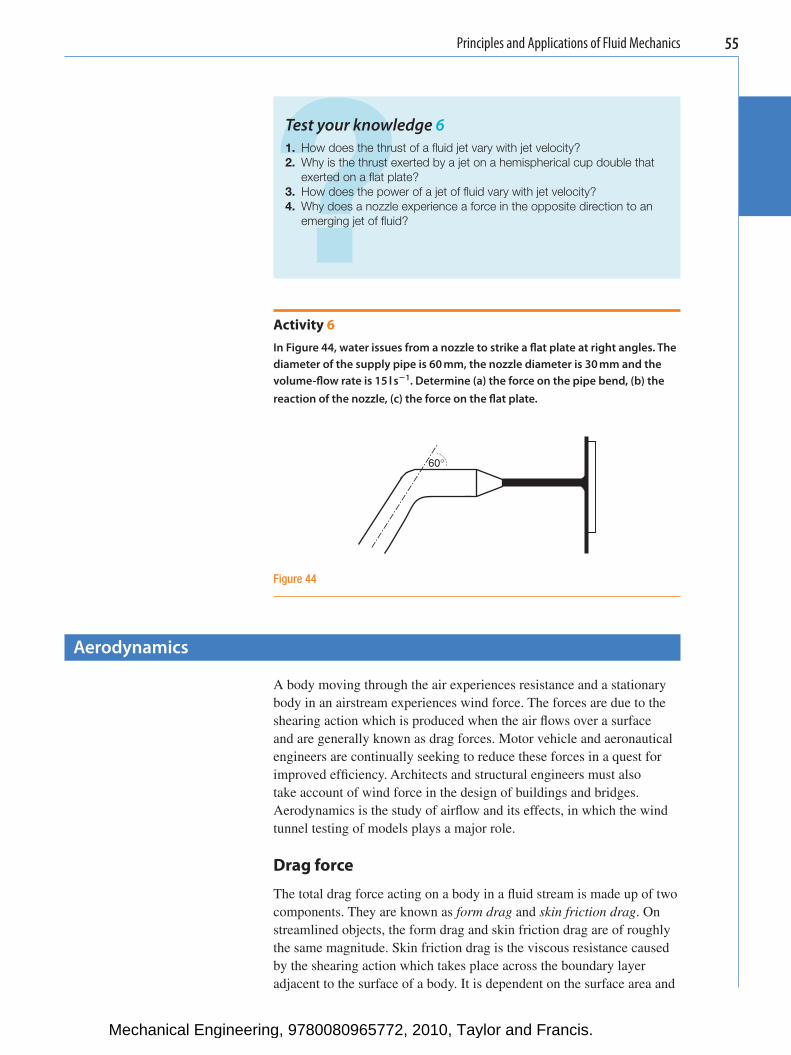
Principles and Applications of Fluid Mechanics 55
Activity 6 In Figure 44 , water issues from a nozzle to strike a fl at plate at right angles. The diameter of the supply pipe is 60 mm, the nozzle diameter is 30 mm and the volume-fl ow rate is 15 l s � 1 . Determine (a) the force on the pipe bend, (b) the reaction of the nozzle, (c) the force on the fl at plate.
? Test your knowledge 6 1. How does the thrust of a fl uid jet vary with jet velocity? 2. Why is the thrust exerted by a jet on a hemispherical cup double that
exerted on a fl at plate? 3. How does the power of a jet of fl uid vary with jet velocity? 4. Why does a nozzle experience a force in the opposite direction to an
emerging jet of fl uid?
Aerodynamics
A body moving through the air experiences resistance and a stationary body in an airstream experiences wind force. The forces are due to the shearing action which is produced when the air fl ows over a surface and are generally known as drag forces. Motor vehicle and aeronautical engineers are continually seeking to reduce these forces in a quest for improved effi ciency. Architects and structural engineers must also take account of wind force in the design of buildings and bridges. Aerodynamics is the study of airfl ow and its effects, in which the wind tunnel testing of models plays a major role.
Drag force
The total drag force acting on a body in a fl uid stream is made up of two components. They are known as form drag and skin friction drag . On streamlined objects, the form drag and skin friction drag are of roughly the same magnitude. Skin friction drag is the viscous resistance caused by the shearing action which takes place across the boundary layer adjacent to the surface of a body. It is dependent on the surface area and
60°
Figure 44
Mechanical Engineering, 9780080965772, 2010, Taylor and Francis.
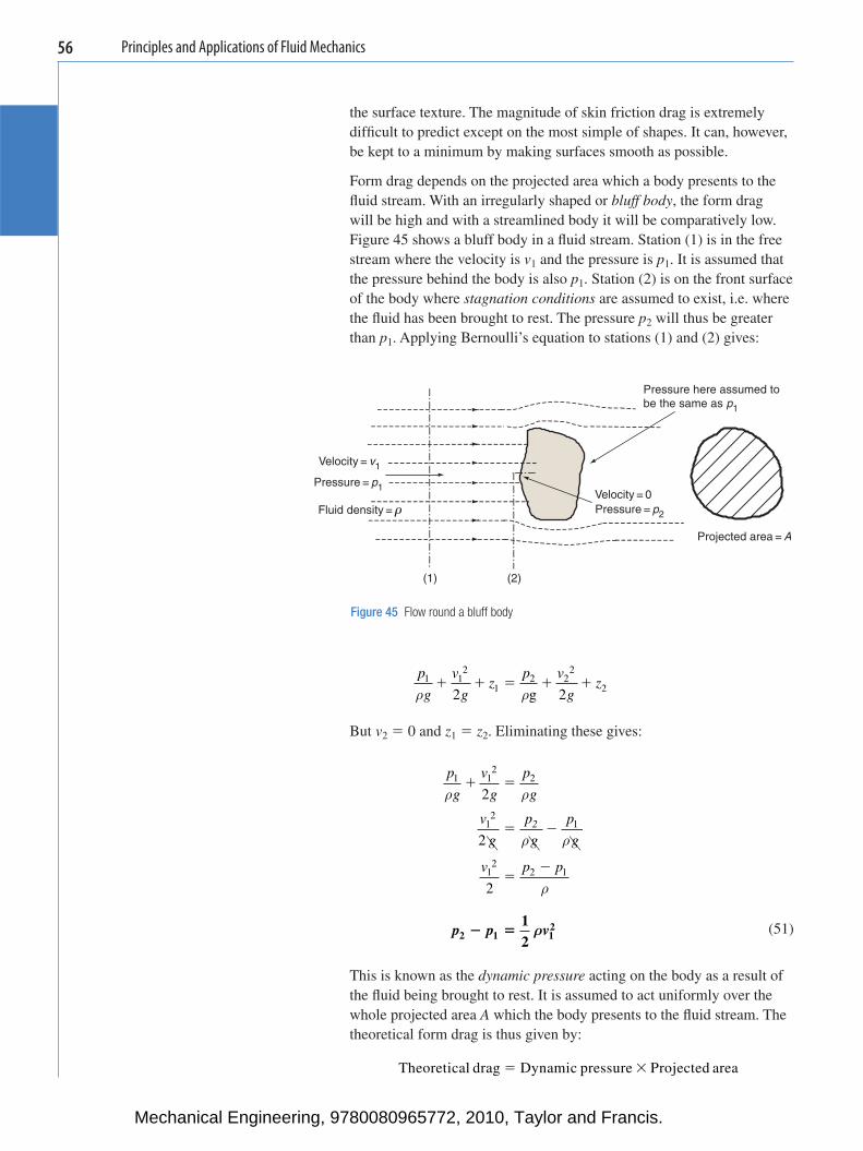
Principles and Applications of Fluid Mechanics56
the surface texture. The magnitude of skin friction drag is extremely diffi cult to predict except on the most simple of shapes. It can, however, be kept to a minimum by making surfaces smooth as possible.
Form drag depends on the projected area which a body presents to the fl uid stream. With an irregularly shaped or bluff body , the form drag will be high and with a streamlined body it will be comparatively low. Figure 45 shows a bluff body in a fl uid stream. Station (1) is in the free stream where the velocity is v 1 and the pressure is p 1 . It is assumed that the pressure behind the body is also p 1 . Station (2) is on the front surface of the body where stagnation conditions are assumed to exist, i.e. where the fl uid has been brought to rest. The pressure p 2 will thus be greater than p 1 . Applying Bernoulli’s equation to stations (1) and (2) gives:
Pressure here assumed tobe the same as p1
Velocity = v1
Pressure = p1Velocity = 0
Fluid density = r Pressure = p2
Projected area = A
(1) (2)
Figure 45 Flow round a bluff body
p
g
v
gz
p v
gz1 1
2
12 2
2
22 g 2ρ ρ� � � � �
But v 2 � 0 and z 1 � z 2 . Eliminating these gives:
p
g
v
g
p
g
v
g
p
g
p
g
v p p
1 12
2
12
1
12
2
2
2
ρ ρ
ρ ρ
ρ
� �
� �
�
2
2 1�
p p v2 1 1
212
� � ρ
(51)
This is known as the dynamic pressure acting on the body as a result of the fl uid being brought to rest. It is assumed to act uniformly over the whole projected area A which the body presents to the fl uid stream. The theoretical form drag is thus given by:
Theoretical drag Dynamic pressure Projected area� �
Mechanical Engineering, 9780080965772, 2010, Taylor and Francis.
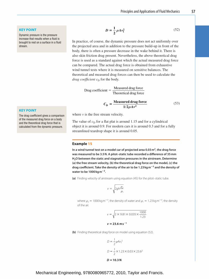
Principles and Applications of Fluid Mechanics 57
D Av�
12 1
2ρ
(52)
In practice, of course, the dynamic pressure does not act uniformly over the projected area and in addition to the pressure build-up in front of the body, there is often a pressure decrease in the wake behind it. There is also skin friction drag present. Nevertheless, the above theoretical drag force is used as a standard against which the actual measured drag force can be compared. The actual drag force is obtained from exhaustive wind tunnel tests where it is measured on sensitive balances. The theoretical and measured drag forces can then be used to calculate the drag coeffi cient c D for the body.
Drag coefficient
Measured drag force
Theoretical drag force�
C
AvD 2
Measured drag force1 2
�/ ρ
(53)
where v is the free stream velocity.
The value of c D for a fl at plat is around 1.15 and for a cylindrical object it is around 0.9. For modern cars it is around 0.3 and for a fully streamlined teardrop shape it is around 0.05.
Example 15 In a wind tunnel test on a model car of projected area 0.03 m 2 , the drag force was measured to be 3.5 N. A pitot–static tube recorded a diff erence of 35 mm H 2 O between the static and stagnation pressures in the airstream. Determine (a) the free stream velocity, (b) the theoretical drag force on the model, (c) the drag coeffi cient. Take the density of the air to be 1.23 kg m � 3 and the density of water to be 1000 kg m � 3 .
(a) Finding velocity of airstream using equation (45) for the pitot–static tube.
v gh� 2 2
1
ρρ
where ρ 2 � 1000 kg m � 3 , the density of water and ρ 1 � 1.23 kg m � 3 , the density of the air.
v � � � �2 9 81 0 035
10001 23
. ..
v � 23 6 1. m s�
(b) Finding theoretical drag force on model using equation (52).
D Av
D
�
� � � �
12
12
1 23 0 03 23 6
12
2
ρ
. . .
D � 10 3. N
KEY POINT Dynamic pressure is the pressure increase that results when a fl uid is brought to rest on a surface in a fl uid stream.
KEY POINT The drag coeffi cient gives a comparison of the measured drag force on a body and the theoretical drag force that is calculated from the dynamic pressure.
Mechanical Engineering, 9780080965772, 2010, Taylor and Francis.
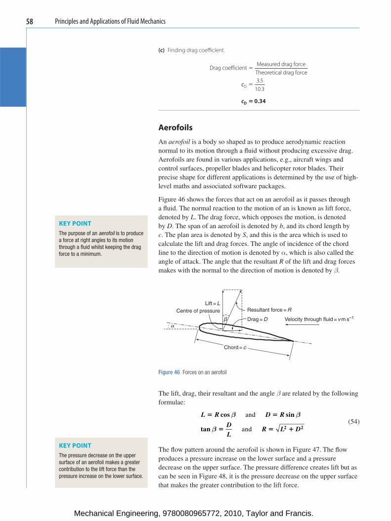
Principles and Applications of Fluid Mechanics58
(c) Finding drag coeffi cient.
Drag coefficientMeasured drag forceTheoretical drag force
�
ccD �3 5
10 3..
cD � 0 34.
Aerofoils
An aerofoil is a body so shaped as to produce aerodynamic reaction normal to its motion through a fl uid without producing excessive drag. Aerofoils are found in various applications, e.g., aircraft wings and control surfaces, propeller blades and helicopter rotor blades. Their precise shape for different applications is determined by the use of high-level maths and associated software packages.
Figure 46 shows the forces that act on an aerofoil as it passes through a fl uid. The normal reaction to the motion of an is known as lift force, denoted by L . The drag force, which opposes the motion, is denoted by D . The span of an aerofoil is denoted by b , and its chord length by c . The plan area is denoted by S , and this is the area which is used to calculate the lift and drag forces. The angle of incidence of the chord line to the direction of motion is denoted by α , which is also called the angle of attack. The angle that the resultant R of the lift and drag forces makes with the normal to the direction of motion is denoted by β .
Lift = L
a
Centre of pressure Resultant force = R
Drag = D Velocity through fluid = v m s–1
Chord = c
b
Figure 46 Forces on an aerofoil
KEY POINT The purpose of an aerofoil is to produce a force at right angles to its motion through a fl uid whilst keeping the drag force to a minimum.
The lift, drag, their resultant and the angle β are related by the following formulae:
L R D R
DL
R L D
� �
� � �
cos sin
tan 2 2
β β
β
and
and
(54)
The fl ow pattern around the aerofoil is shown in Figure 47 . The fl ow produces a pressure increase on the lower surface and a pressure decrease on the upper surface. The pressure difference creates lift but as can be seen in Figure 48 , it is the pressure decrease on the upper surface that makes the greater contribution to the lift force.
KEY POINT The pressure decrease on the upper surface of an aerofoil makes a greater contribution to the lift force than the pressure increase on the lower surface.
Mechanical Engineering, 9780080965772, 2010, Taylor and Francis.
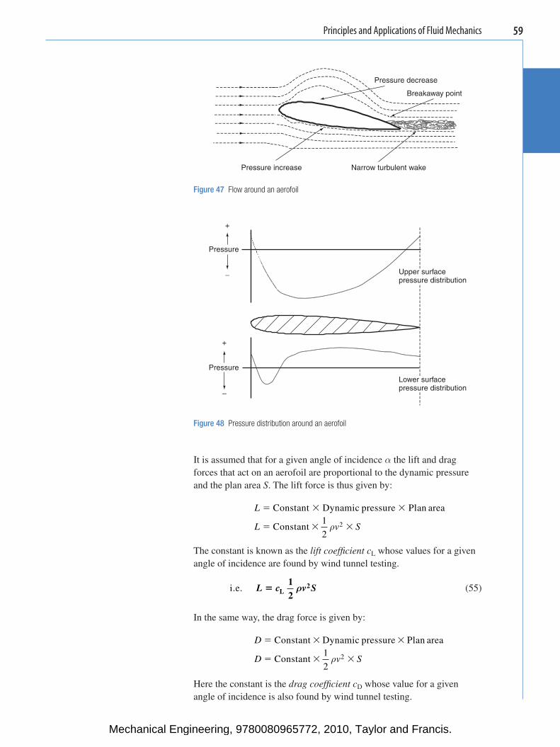
Principles and Applications of Fluid Mechanics 59
It is assumed that for a given angle of incidence α the lift and drag forces that act on an aerofoil are proportional to the dynamic pressure and the plan area S . The lift force is thus given by:
L
L v S
� � �
� � �
Constant Dynamic pressure Plan area
Constant1
22ρ
The constant is known as the lift coeffi cient c L whose values for a given angle of incidence are found by wind tunnel testing.
i.e. L c v S� L
212
ρ
(55)
In the same way, the drag force is given by:
D
D v S
� � �
� � �
Constant Dynamic pressure Plan area
Constant1
22ρ
Here the constant is the drag coeffi cient c D whose value for a given angle of incidence is also found by wind tunnel testing.
Pressure decrease
Breakaway point
Pressure increase Narrow turbulent wake
Figure 47 Flow around an aerofoil
+
+
_ Upper surface pressure distribution
Pressure
Pressure
Lower surfacepressure distribution
–
Figure 48 Pressure distribution around an aerofoil
Mechanical Engineering, 9780080965772, 2010, Taylor and Francis.
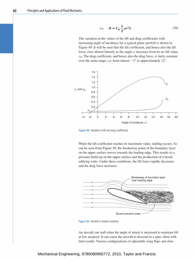
Principles and Applications of Fluid Mechanics60
i.e. D C v S� D
212
ρ
(56)
The variation in the values of the lift and drag coeffi cients with increasing angle of incidence for a typical plane aerofoil is shown in Figure 49 . It will be seen that the lift coeffi cient, and hence also the lift force, rises almost linearly as the angle α increases from its no-lift value, α 0 . The drag coeffi cient, and hence also the drag force, is fairly constant over the same range, i.e. from almost � 2 ° to approximately 12 ° .
1.6
1.4
1.2
1.0cL and cD
cL
cD
0.8
0.6
0.4
0.2
–2°–4° 0 4°2° 6° 8° 10° 12° 14° 16° 18° 20°
Angle of incidence, a°
a0
Figure 49 Variation of lift and drag coeffi cients
Breakaway of boundary layernear leading edge
Broad turbulent wake
Figure 50 Aerofoil in stalled condition
When the lift coeffi cient reaches its maximum value, stalling occurs. As can be seen from Figure 50 , the breakaway point of the boundary layer on the upper surface moves towards the leading edge. This results in a pressure build-up on the upper surface and the production of a broad eddying wake. Under these conditions, the lift force rapidly decreases and the drag force increases.
An aircraft can stall when the angle of attack is increased to maintain lift at low airspeed. It can cause the aircraft to descend in a spin, often with fatal results. Various confi gurations of adjustable wing fl aps and slots
Mechanical Engineering, 9780080965772, 2010, Taylor and Francis.
Principles and Applications of Fluid Mechanics 61
have been developed which enable aircraft to maintain lift at relatively low take-off and landing speeds. If you are able to secure an airline seat with a view of the wing, you will be able to see these in operation.
When an aircraft is travelling at a steady speed in level fl ight, the thrust of the engines must be equal and opposite to the drag force and the lift must be equal and opposite to its weight. The power required from the engines of a jet aircraft is the product of the thrust, F N, and the airspeed, v m s � 1 .
i.e. Power Thrust Airspeed� �
But the thrust is equal and opposite to the drag force, D .
Power � Dv (57)
In the case of propeller-driven aircraft, the propeller effi ciency, η , has to be taken into account and the required shaft output power is given by:
Power �
Dvη
(58)
Example 16 The lift surfaces of an aircraft have a plan area of 60 m 2 and the wing loading is 2 kN m � 2 . The propellers are 75% effi cient and the lift and drag coeffi cients are in the ratio 11:1. The density of the air is 1.27 kg m � 3 . Determine (a) the lift and drag coeffi cients, (b) the engine power required to propel the aircraft in level fl ight at a steady airspeed of 500 km h � 1 .
(a) Finding airspeed in m s � 1 .
v � �500
1000602
v � �139 m s 1
Finding lift force.
L
L
�
�
Wing loading Wing area�
� �2 10 603
L � �120 10 N or 120 kN3
Finding lift coeffi cient.
L c v S
cL
v S
�
� �� �
� �
L
L
12
2 2 120 101 27 139 60
2
2
3
2
ρ
ρ .
cL 0.163�
Mechanical Engineering, 9780080965772, 2010, Taylor and Francis.
Principles and Applications of Fluid Mechanics62
? Test your knowledge 7 1. Distinguish between skin friction drag and form drag. 2. How is the drag coeffi cient defi ned for a body in a fl uid stream? 3. How is the lift force on an aerofoil produced? 4. What occurs during stalling? 5. How is engine power calculated for an aircraft travelling at a steady
speed in level fl ight?
Activity 7 A rectangular aerofoil of chord 300 mm and span 1.5 m is tested in a wind tunnel in which the airspeed is 60 m s � 1 and the air density is 1.3 kg m � 3 . The resultant force on the aerofoil is measured to be 850 N at an angle of 4 ° to the vertical axis of lift. Determine the lift and drag coeffi cients.
A propeller-driven aircraft of mass 10 tonnes has lift surfaces with the same characteristics. What will be the engine power required to maintain an airspeed of 450 km h � 1 in level fl ight if the propeller effi ciency is 80%?
Finding drag coeffi cient.
cc
cc
L
D
DL
�
� �
11
110 163
11.
cD � 0 0148.
(b) Finding drag force.
cc
LD
DL
L
D
� �
� ��
11
11120 10
11
3
D � �10 9 10 10 93. .N kNor
Finding engine power required.
Power
Power
�
�� �
Dvη
10 9 10 1390 75
3..
Power W MW� �2 02 10 2 026. .or
Mechanical Engineering, 9780080965772, 2010, Taylor and Francis.
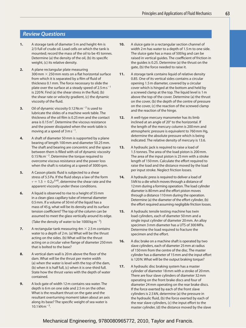
Principles and Applications of Fluid Mechanics 63
Review Questions
1. A storage tank of diameter 5 m and height 4m is 2/3 full of crude oil. Load cells on which the tank is mounted; record the mass of the oil to be 45 tonnes. Determine (a) the density of the oil, (b) its specifi c weight, (c) its relative density.
2. A plane rectangular plate measuring 300 mm � 250 mm rests on a fl at horizontal surface from which it is separated by a fi lm of fl uid of thickness 0.1 mm. The force necessary to slide the plate over the surface at a steady speed of 2.5 m s � 1 is 220 N. Find (a) the shear stress in the fl uid, (b) the shear rate or velocity gradient, (c) the dynamic viscosity of the fl uid.
3. Oil of dynamic viscosity 0.12 Ns m � 2 is used to lubricate the slides of a machine work table. The thickness of the oil fi lm is 0.25 mm and the contact area is 0.15 m 2 . Determine the viscous resistance and the power dissipated when the work table is moving at a speed of 3 m s � 1 .
4. A shaft of diameter 50 mm is supported by a plane bearing of length 100 mm and diameter 50.25 mm. The shaft and bearing are concentric and the space between them is fi lled with oil of dynamic viscosity 0.15 Ns m � 2 . Determine the torque required to overcome viscous resistance and the power loss when the shaft is rotating at a speed of 3000 rpm.
5. A Casson plastic fl uid is subjected to a shear stress of 5.5 Pa. If the fl uid obeys a law of the form τ � 1.5 � 0.2 µ 0.45 , determine the shear rate and the apparent viscosity under these conditions.
6. A liquid is observed to rise to a height of 55 mm in a clean glass capillary tube of internal diameter 0.5 mm. If a volume of 50 ml of the liquid has a mass of 45 g, what will be its density and its surface tension coeffi cient? The top of the column can be assumed to meet the glass vertically around its edge.
(Take the density of water to be 1000 kg m � 3 )
7. A rectangular tank measuring 4m � 2.5 m contains water to a depth of 2 m. (a) What will be the thrust acting on the sides. (b) What will be the thrust acting on a circular valve fl ange of diameter 250 mm that is bolted to the base?
8. A vertical dam wall is 20 m above the fl oor of the dam. What will be the thrust per metre width (a) when the water is level with the top of the dam, (b) when it is half full, (c) when it is one-third full. State how the thrust varies with the depth of water contained.
9. A lock gate of width 12 m contains sea water. The depth is 6 m on one side and 2.5 m on the other. What is the resultant thrust on the gate and the resultant overturning moment taken about an axis along its base? The specifi c weight of sea water is 10.1 kN m � 3 .
10. A sluice gate in a rectangular section channel of width 2 m has water to a depth of 1.5 m to one side. The sluice gate has a mass of 500 kg and can be raised in vertical guides. The coeffi cient of friction in the guides is 0.25. Determine (a) the thrust on the gate, (b) the force needed to raise it.
11. A storage tank contains liquid of relative density 0.85. One of its vertical sides contains a circular opening 1.5 m diameter, covered by a circular cover which is hinged at the bottom and held by a screwed clamp at the top. The liquid level is 1 m above the top of the cover. Determine (a) the thrust on the cover, (b) the depth of the centre of pressure on the cover, (c) the reaction of the screwed clamp and the reaction of the hinge.
12. A well-type mercury manometer has its limb inclined at an angle of 20° to the horizontal. If the length of the mercury column is 200 mm and atmospheric pressure is equivalent to 760 mm Hg, determine the absolute pressure which is being indicated. The relative density of mercury is 13.6.
13. A hydraulic jack is required to raise a load of 1.5 tonnes. The area of the load piston is 200 mm. The area of the input piston is 25 mm with a stroke length of 150 mm. Calculate the eff ort required to raise the load and the distance moved by the load per input stroke. Neglect friction losses.
14. A hydraulic press is required to deliver a load of 5 kN to a die which moves through a distance of 12 mm during a forming operation. The load cylinder diameter is 80 mm and the eff ort piston moves through a distance 110 mm during the operation. Determine (a) the diameter of the eff ort cylinder, (b) the eff ort required assuming negligible friction losses.
15. A hydraulic tensile testing machine has twin load cylinders, each of diameter 50 mm and a single input cylinder of diameter 20 mm. An alloy specimen 3 mm diameter has a UTS of 300 MPa. Determine the load required to fracture the specimen and the eff ort.
16. A disc brake on a machine shaft is operated by two slave cylinders, each of diameter 25 mm at radius of 150 mm from the centre of the disc. The master cylinder has a diameter of 15 mm and the input eff ort is 120 N. What will be the output braking torque?
17. A hydraulic disc braking system has a master cylinder of diameter 18 mm with a stroke of 20 mm. There are four slave cylinders of diameter 32 mm operating on the front brake discs and four of diameter 24 mm operating on the rear brake discs. If the force exerted by each of the front slave cylinders is 2.5 kN, determine (a) the pressure in the hydraulic fl uid, (b) the force exerted by each of the rear slave cylinders, (c) the input eff ort to the master cylinder, (d) the distance moved by the slave
Mechanical Engineering, 9780080965772, 2010, Taylor and Francis.
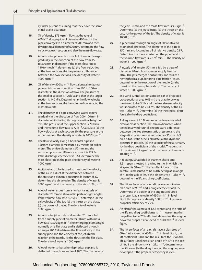
Principles and Applications of Fluid Mechanics64
cylinder pistons assuming that they have the same initial brake clearance .
18. Oil of density 875 kg m � 3 fl ows at the rate of 400 l s � 1 along a pipe of diameter 400 mm. If the pipe converges to a diameter of 200 mm and then diverges to a diameter of 600 mm, determine the fl ow velocity at each section and also the mass-fl ow rate.
19. A horizontal pipe which runs full of water diverges gradually in the direction of the fl ow from 150 to 300 mm in diameter. If the mass-fl ow rate is 110 tonnes h � 1 , determine (a) the fl ow velocities at the two sections, (b) the pressure diff erence between the two sections. The density of water is 1000 kg m � 3 .
20. Oil of density 800 kg m � 3 fl ows along a horizontal pipe which varies in section from 100 to 150 mm diameter in the direction of fl ow. The pressure at the smaller section is 126 kPa and that at the larger section is 140 kPa. Determine (a) the fl ow velocity at the two sections, (b) the volume-fl ow rate, (c) the mass-fl ow rate.
21. The diameter of a pipe conveying water tapers gradually in the direction of fl ow 200–100 mm in diameter whilst falling through a vertical height of 9 m. The pressure at the upper section is 210 kPa and the volume-fl ow rate is 72 l s � 1 . Calculate (a) the fl ow velocity at each section, (b) the pressure at the upper section. The density of water is 1000 kg m � 3 .
22. The fl ow velocity along a horizontal pipeline 120 mm diameter is measured by means an orifi ce meter. The orifi ce diameter is 50 mm and the recorded pressure diff erence across it is 12 kPa. If the discharge coeffi cient is 0.64, determine the mass-fl ow rate in the pipe. The density of water is 1000 kg m � 3 .
23. A pitot–static tube is used to measure the velocity of the air in a duct. If the diff erence between the static and dynamic pressures is 30 mm H 2 O, determine the air velocity. The density of water is 1000 kg m � 3 and the density of the air is 1.2 kg m � 3 .
24. A jet of water issues from a horizontal nozzle of diameter 25 mm to strike a fl at plate at right angles. If the volume-fl ow rate is 7.5 l s � 1 , determine (a) the exit velocity of the jet, (b) the thrust on the plate, (c) the power of the jet. The density of water is 1000 kg m � 3 .
25. A horizontal jet nozzle of diameter 20 mm is fed from a supply pipe of diameter 80 mm with mass-fl ow rate is 500 kg min � 1 . The emerging jet impinges normally on a fl at plate and is defl ected through an angle 90 ° . Calculate (a) the fl ow velocity in the supply pipe and the velocity of the jet, (b) the reaction o the nozzle, (c) the thrust on the fl at plate. The density of water is 1000 kg m � 3 .
26. A jet of water strikes a hemispherical cup and is defl ected through an angle of 180 ° . The diameter of
the jet is 30 mm and the mass-fl ow rate is 9.5 kg s � 1 . Determine (a) the jet velocity, (b) the thrust on the cup, (c) the power of the jet. The density of water is 1000 kg m � 3 .
27. A pipe turns through an angle of 60 ° relative to its original direction. The diameter of the pipe is 150 mm and it contains oil of relative density 0.87. Determine the force exerted on the pipe bend if the volume-fl ow rate is 5.3 m 3 min � 1 . The density of water is 1000 kg m � 3 .
28. A nozzle of diameter 50 mm is fed by a pipe of diameter 90 mm from a water supply head of 30 m. The jet emerges horizontally and strikes a hemispherical cup. Ignoring pipe friction losses, determine (a) the reaction of the nozzle, (b) the thrust on the hemispherical cup. The density of water is 1000 kg m � 3 .
29. In a wind tunnel test on a model car of projected cross-sectional area 0.03 m 2 , the drag force was measured to be 3.1 N and the free stream velocity was indicated to be 22.1 ms. The density of the air was 1.2 kg m � 3 . Determine (a) the theoretical drag force, (b) the drag coeffi cient.
30. A drag force of 2.1 N was recorded on a model of circular cross-section, 100 mm in diameter, when tested in a wind tunnel. The pressure diff erence between the free stream static pressure and the stagnation pressure was recorded as 35 mm H 2 O on a pitot–static tube. Calculate (a) the dynamic pressure in pascals, (b) the velocity of the airstream, (c) the drag coeffi cient of the model. The density of the air was1.2 kg m � 3 and the density of water is 1000 kg m � 3 .
31. A rectangular aerofoil of 300 mm chord and 1.5 m span is tested in a wind tunnel in which the airspeed is 60 m s � 1 . The resultant force on the aerofoil is measured to be 850 N acting at an angle of 4 ° to the axis of lift. If the air density is 1.3 kg m � 3 , determine the lift and drag coeffi cients.
32. The lift surfaces of an aircraft have an equivalent plan area of 90 m 2 and a drag coeffi cient of 0.05. Determine the power of the engines required to propel it at a velocity of 450 km h � 1 in level fl ight through air of density 1.3 kg m � 3 . Assume a propeller effi ciency of 75%.
33. An aircraft has a mass of 12.2 tonnes and the ratio of the lift and drag coeffi cients is 11:1. Assuming the propellers to be 75% effi cient, determine the engine power to propel it at a speed of 500 km h � 1 in level fl ight.
34. The lift surfaces of an aircraft have a plan area of 60 m 2 . At a speed of 450 km h � 1 in level fl ight, the lift coeffi cient is 0.8 and the resultant thrust on the lift surfaces is inclined at an angle of 4.5 ° to the axis of lift. If the air density is 1.2 kg m � 3 , determine (a) the lift force, (b) the drag force, (c) the engine power developed if the propeller effi ciency is 75%.
Mechanical Engineering, 9780080965772, 2010, Taylor and Francis.