Embed Size (px)
Citation preview

Mechanical Characterisation and Computational Modelling of
Spinal Ligaments
Miss Ayesha Bint-E-Siddiq
Submitted in accordance with the requirements for the degree of
Doctor of Philosophy
The University of Leeds
Institute of Medical and Biological Engineering
School of Mechanical Engineering
July, 2019

The candidate confirms that the work submitted is her own and that appropriate
credit has been given where reference has been made to the work of others.
This copy has been supplied on the understanding that it is copyright material
and that no quotation from the thesis may be published without proper
acknowledgement.
The right of Miss Ayesha Bint-E-Siddiq to be identified as Author of this work
has been asserted by her in accordance with the Copyright, Designs and
Patents Act 1988.
© 2019 The University of Leeds and Miss Ayesha Bint-E-Siddiq

For my Mum & Dad, Samina & Siddiq

i
Acknowledgements
Over the course of my PhD, I have had the honour of working with some
incredible people without whom I would not be here today. It is an
acknowledgement to these people, who have supported me throughout this
journey with their continuous advice, help and guidance. I would also like to
express my gratitude towards people without whom I would not have come this
far.
First and foremost, I would like to thank my primary supervisor Professor Ruth
Wilcox, who has always been ever so helpful. Her cheerful and kind personality
has lifted my morale on many occasions. Every time I needed some help or
advice, she was just an email away. She has always had something
constructive to add to even the most ‘naïve’ and ‘silly’ questions I have had and
hence why I never hesitated in raising any concerns. I would also like to thank
my co-supervisors Dr Alison Jones and Dr Marlène Mengoni who have also
contributed immensely to my progress and have always given very thorough
and timely feedback. Thank you all for your help and patience throughout the
years. Words cannot do justice to the amount of gratitude I have, I could not
have asked for a better team. It has been an incredible journey and your
support is much appreciated.
I would like to extend my thanks to Phil Wood, Irvin Homan and Lee Whetherill
and the rest of the technical staff within the School of Mechanical Engineering
for their support and guidance. Special thanks to Dr Nagitha Wijayathunga
without his help the human tissue work would not have been possible. His
willingness to make time to help me when asked is commendable. Thanks to all
my researcher friends for not only providing good office banter but also
extending a helping hand whenever needed.
I sincerely thank my family without whom I would not be here today. In
particular, my Mum and Dad, Samina and Siddiq, I have no words to
acknowledge the sacrifices you made to make me successful. Your hard work
and can-do attitude has always been an inspiration to me. Mum, your belief in
me has kept me going even at difficult times. Thanks to my wonderful sister,
Ajwa, for your patience and willingness to lend an ear whenever I needed a
sounding board. Thanks to my lovely sisters Fozia and Aisha for your constant
entertainment and support that helped me through low-moments. Special
thanks to my amazing brothers Omar, Salman and Zaid for always believing in
me. Your support and encouragement has lifted my spirits on many occasions.

ii
Sincere and heart-felt gratitude to Ma (Shirin), Pa (Rashid) and Yasir for being
ever so kind and thoughtful. And last but not the least, my wonderful husband,
Yasiin, who have provided me with a listening ear whenever needed and have
helped me get through hard times. This journey would not have been possible
without you all and for that I am grateful to you all from the bottom of my heart.

iii
Abstract
Low back pain is a common complaint in people of all ages. The long-term
success rates of many surgical devices to treat the spine have been relatively
low and improved methods of pre-clinical testing of these devices are therefore
needed. Sheep spine models are commonly employed in pre-clinical research
studies for the evaluation of spinal devices. The anterior and posterior
longitudinal ligaments (ALL and PLL) provide passive stability to the spine,
however, limited studies have been conducted to characterise the mechanical
properties of the ovine longitudinal ligaments or compare them to the human.
Moreover, previous studies have derived material properties for the human ALL
and PLL directly from force-displacement data, assuming uniform cross
sectional area and length, and these values have been used extensively in
finite element models of the spine for the analysis of clinical interventions.
The aim of this study was to develop a methodology to test and compare the
stiffness of human and ovine spinal longitudinal ligaments and to uniquely
combine experimental and specimen-specific finite element (FE) modelling
approaches to determine the ligament mechanical properties.
The methodology was developed on ovine thoracic spines and then applied to
human thoracic spines. The spines were dissected into functional spinal units
(FSUs) with the posterior elements removed and imaged under micro
computed tomography (µCT). The specimens were sectioned through the disc
to leave only either the ALL or PLL intact and tested in tension to determine the
stiffness. The µCT images from each FSU were used to build specimen-
specific FE models of the ligaments and bony attachments. Hyper-elastic
material models were used to represent the ligament behaviour. Initial values
for the material model were derived using mean cross sectional area (CSA)
and length (L), with the assumption that ligament was uniaxially loaded. The
parameters were then iteratively changed until a best fit to the corresponding
experimental load-displacement data was found for each specimen.
The stiffness of the ligaments for the ovine specimens were found to be higher
than for the human specimens. This may have implications for the use of ovine
FSUs for preclinical testing of devices. There was poor agreement between the
material parameters derived from FE models and the initial values derived by
assuming a mean CSA and L. This work demonstrates that a specimen-specific
image-based approach needs to be applied to derive the elastic properties of
the ligaments due to their non-uniform shape and cross-sectional area.

iv
Table of Contents
Acknowledgements ...................................................................................... i
Abstract ....................................................................................................... iii
Abbreviations ............................................................................................ xix
Chapter 1 Introduction and Literature Review .......................................... 1
1.1 Introduction ....................................................................................... 1
1.2 Literature Review ............................................................................. 3
1.2.1 Biomechanically Relevant Human Spinal Anatomy ................. 3
1.2.2 Comparison of Human and Ovine Spine Anatomy ................ 15
1.2.3 Biomechanics of Spine .......................................................... 18
1.2.4 Biomechanics of Spinal Ligaments ....................................... 19
1.2.5 Experimental Testing of Spinal Ligaments ............................ 23
1.2.6 Finite Element Modelling of Ligaments ................................. 42
1.2.7 Material models for soft tissue modelling .............................. 52
1.3 Study Motivation, Aim and Objectives ............................................ 57
Chapter 2 Experimental Methods Development and Results for Ovine Longitudinal Ligaments .................................................................... 60
2.1 Introduction ..................................................................................... 60
2.2 Ovine Ligament Anatomy ............................................................... 60
2.2.1 Introduction ........................................................................... 60
2.2.2 Methods ................................................................................ 60
2.2.3 Results .................................................................................. 61
2.2.4 Discussion ............................................................................. 62
2.3 General Materials and Methods ..................................................... 64
2.3.1 Specimens ............................................................................ 64
2.3.2 Dissection.............................................................................. 64
2.3.3 Potting of Specimens ............................................................ 65
2.3.4 Mechanical Testing Setup ..................................................... 66
2.3.5 Load and Displacement Limits .............................................. 67
2.4 Testing Protocol ............................................................................. 68
2.4.1 Introduction ........................................................................... 68
2.4.2 Method Development ............................................................ 69
2.4.3 Method Adopted .................................................................... 75
2.5 Methods of Data Analysis ............................................................... 77

v
2.6 Results and Analysis ...................................................................... 80
2.7 Discussion ...................................................................................... 84
2.7.1 Discussion of testing methods and results ............................ 84
2.7.2 Comparison to published human data ................................... 86
2.7.3 Summary ............................................................................... 87
Chapter 3 Computational Methods Development and Results for Ovine Longitudinal Ligaments .................................................................... 88
3.1 Introduction ..................................................................................... 88
3.2 Imaging Specimens ........................................................................ 88
3.2.1 Introduction ........................................................................... 88
3.2.2 Imaging Protocol ................................................................... 89
3.2.3 Use of Radiopaque Gel ......................................................... 90
3.3 Determination of Ligament Thickness over Disc ............................ 92
3.3.1 Introduction ........................................................................... 92
3.3.2 Needle Indentation Test ........................................................ 92
3.3.3 Photographic Image Analysis ................................................ 95
3.3.4 Discussion ............................................................................. 97
3.4 Image Segmentation ...................................................................... 97
3.4.1 Images Pre-processing ......................................................... 97
3.4.2 Segmentation of the Bone ..................................................... 98
3.4.3 Segmentation of the Ligament .............................................. 99
3.5 Image Downsampling ................................................................... 101
3.6 Finite Element Method Development ........................................... 105
3.6.1 Sensitivity Analysis .............................................................. 105
3.6.2 Summary ............................................................................. 122
3.7 Final Methods of FE Modelling ..................................................... 123
3.7.1 FE Modelling of the ALL ...................................................... 123
3.7.2 FE Modelling of the PLL ...................................................... 124
3.8 Initial Results for the ALL Model with Material Data derived by Assuming Uniform Uniaxial Conditions......................................... 125
3.9 Method of Tuning the Material Properties ..................................... 127
3.9.1 Theoretical Considerations.................................................. 128
3.9.2 Effect of Varying Input Parameters ..................................... 130
3.9.3 Parameter Tuning Methods ................................................. 131
3.9.4 Parameter Tuning Results .................................................. 135
3.10 Discussion .................................................................................... 137

vi
Chapter 4 Application of Experimental & Computational Methods to Human Longitudinal Ligaments ..................................................... 141
4.1 Introduction ................................................................................... 141
4.2 Methodology ................................................................................. 141
4.2.1 Magnetic Resonance Imaging ............................................. 141
4.2.2 Dissection............................................................................ 142
4.2.3 Specimen preparation and testing ....................................... 142
4.2.4 Computational Modelling ..................................................... 143
4.3 Results ......................................................................................... 144
4.3.1 Comparison of Human and Ovine Thoracic Spine .............. 144
4.3.2 Visual Observations, MRI and Photographic Images .......... 147
4.3.3 Mechanical Testing ............................................................. 149
4.3.4 FE modelling and material parameter tuning ...................... 152
4.3.5 Comparison of Material Models ........................................... 155
4.3.6 Comparison between Coefficients ....................................... 157
4.3.7 Comparison by spine and by level ...................................... 158
4.3.8 Comparison with other computational data ......................... 162
4.4 Discussion .................................................................................... 165
4.4.1 Discussion of Experimental Results and Visual Observations 165
4.4.2 Discussion of Finite Element Modelling ............................... 167
4.4.3 Comparison and Analysis of Material Parameters .............. 168
4.4.4 Variability across Individual Spines and Spinal Levels ........ 170
4.4.5 Comparison with Published Human Data ............................ 171
4.4.6 Conclusion .......................................................................... 176
Chapter 5 Discussion .............................................................................. 177
5.1 Introduction ................................................................................... 177
5.2 Comparison of the stiffness values for human and ovine longitudinal ligaments ...................................................................................... 178
5.3 Comparison of the material parameters of human and ovine ligaments ...................................................................................... 181
5.4 Comparison with the literature on other ligaments ....................... 183
5.5 Limitations and future work ........................................................... 186
5.5.1 Limitations ........................................................................... 186
5.5.2 Future recommendations .................................................... 187
5.6 Conclusion .................................................................................... 188

vii
List of References .................................................................................... 190

viii
List of Tables
Table 1.1: Comparison of Human and Ovine Spine Vertebrae (Adapted from Wilke, et al., 1997). .................................................................... 17
Table 1.2: Mechanical properties of anterior longitudinal ligament (ALL). .................................................................................................. 34
Table 1.3: Mechanical properties of posterior longitudinal ligament (PLL).................................................................................................... 35
Table 1.4: Mechanical properties of ligamentum flavum (LF) ................ 36
Table 1.5: Mechanical properties of intertransverse ligament (ITL) ...... 37
Table 1.6: Mechanical properties of interspinous ligament (ISL) .......... 38
Table 1.7: Mechanical properties of supraspinous ligament (SSL) ....... 39
Table 1.8: Mechanical properties of joint capsular ligament (JCL) ....... 39
Table 1.9: Material properties used by researchers in FE studies including the cross sectional area (CSA), Young’s moduli (E) and transition strains (ɛ). where, E1, E2 and E3 represent the Young’s moduli of the polygonal stress-strain function while ɛ1, ɛ2 and ɛ3 are the corresponding transitions strains separating the Young’s moduli with ɛ3 being the maximum strain of the physiological range. .................................................................................................. 45
Table 1.10: Comparison of different elements types used by researchers in FE modelling of lumbar spine ................................. 49
Table 1.11: List of various hyperelastic material models and their respective Abaqus implementation strain energy potentials which can be used for FE modelling of ligaments. (ABAQUS, 2011) ....... 55
Table 2.1: Initial ovine spine dissection comparing images of the ligaments identified in both lumbar and thoracic region with the cranial end on the right side of all the images. ............................... 62
Table 2.2: The ‘toe region’ (k1) and final ‘linear region’ (k2) stiffness values, calculated by fitting least squares slopes to the post-processed load displacement curves of ALL, alongside the level and the spine the specimen was obtained from. The whole group mean and standard deviation (S.D.) are also shown. ..................... 82
Table 2.3: The ‘toe region’ (k1) and final ‘linear region’ (k2) stiffness values, calculated by fitting least squares slopes to the post-processed load displacement curves of PLL, alongside the level and the spine the specimen was obtained from. The whole group mean and standard deviation (S.D.) are also shown. ..................... 83
Table 3.1: µCT scanner settings used on a SCANCO µCT100 device to image FSUs with the ligaments intact.............................................. 89

ix
Table 3.2: Thickness values of a ligament obtained after conversion from pixels to millimetres over disc and corresponding bone regions. ............................................................................................... 96
Table 3.3: An example of image downsampling from original resolution of 0.074mm to how the optimum of 0.6mm was arrived at. .......... 102
Table 3.4: The various downsampling algorithms along with the volume of ligament and the final model generated by each. ..................... 103
Table 3.5: Geometric parameters used for the development of idealised rectangular models of ligament. ..................................................... 106
Table 3.6: Contour plots obtained for Rec_A, Rec_B and Real_A alongside the scale in mm showing displacement in the direction of stretch (U3) .................................................................................. 109
Table 3.7: The displacements in the x (U1), y (U2) and z (U3) directions obtained for Rec_C and Rec_D showing that the greatest variation occurs over the section corresponding to the disc region. ......... 114
Table 3.8: Material coefficient values obtained for the various material models used for modelling ALL. .................................................... 127
Table 3.9: The final material coefficients obtained as a result of material tuning. ............................................................................................... 136
Table 4.1: List of specimens according to the level of the spine and the ligament tested alongside the gender and age for each donor. .. 143
Table 4.2: Differences in the thickness of the ALL across the three spines with white lines drawn over the images of specimens (row 1) to highlight the edges of the ligament while the unaltered images are presented in 2nd row showing that Spine 3 have the thickest and Spine 1 the thinnest ALL. .......................................... 148
Table 4.3: The ‘toe region’ (k1) and ‘linear region’ (k2) stiffness values calculated by fitting least squares slopes to the post-processed load displacement curves of the ALL specimens. The level and the spine the specimen was obtained from are indicated in the specimen name. ............................................................................... 150
Table 4.4: The ‘toe region’ (k1) and ‘linear region’ (k2) stiffness values calculated by fitting least squares slopes to the post-processed load displacement curves of the PLL. The level and the spine the specimen was obtained from are indicated in the specimen name. ........................................................................................................... 151
Table 4.5: Percentage difference between experimental input and specimen-specific FE-output using material parameters derived by the in-built Abaqus calibration code assuming mean cross-sectional area and length for all the specimens of ALL and PLL. ........................................................................................................... 153
Table 4.6: Calibrated material parameters for Ogden (N=1) and hyperfoam material models obtained as a result of the material optimisation procedure undertaken on the specimen-specific FE models by the author....................................................................... 155

x
Table 4.7: Estimated values of the stress-strain gradient at 12% strain (E) from the material parameters for all the specimens of ALL (n=7). ................................................................................................. 163
Table 4.8: Estimated values of the stress-strain gradient at 20% strain (E) from the material parameters for all the specimens of PLL (n=7). ................................................................................................. 164
Table 5.1: Results of ANOVA performed to compare the stiffness between human and ovine ALL and PLL specimens separately for the toe-region (K1) and linear-region (K2) stiffness. .................... 180

xi
List of Figures
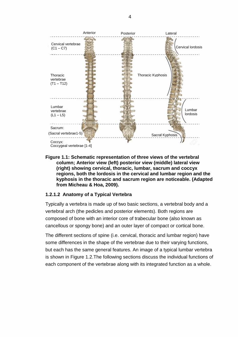
Figure 1.1: Schematic representation of three views of the vertebral column; Anterior view (left) posterior view (middle) lateral view (right) showing cervical, thoracic, lumbar, sacrum and coccyx regions, both the lordosis in the cervical and lumbar region and the kyphosis in the thoracic and sacrum region are noticeable. (Adapted from Micheau & Hoa, 2009). ............................................... 4
Figure 1.2: A typical lumbar vertebrae showing (a) top view and (b) lateral view. (Adapted from Emory University, 1997)........................ 5
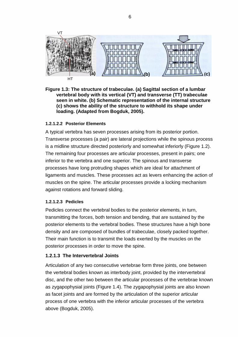
Figure 1.3: The structure of trabeculae. (a) Sagittal section of a lumbar vertebral body with its vertical (VT) and transverse (TT) trabeculae seen in white. (b) Schematic representation of the internal structure (c) shows the ability of the structure to withhold its shape under loading. (Adapted from Bogduk, 2005). ....................... 6
Figure 1.4: The motion of intervertebral joints in flexion and extension. (Adapted from PainNeck.com, 2010). ................................................. 7
Figure 1.5: Schematic representations of the intervertebral disc. (a) The anatomical regions in a mid-sagittal cross-section. (b) A three dimensional view of the disc illustrating annulus fibrosus lamellar structure. (Adapted from Smith et al. 2011) ....................................... 8
Figure 1.6: A view of spinal ligaments from the front of the vertebral bodies with the top body excised (adapted from Eidelson, 2012). 10
Figure 1.7: A schematic of micro to macro level structure of a typical ligament (adapted from Panagos, 2015). ......................................... 13
Figure 1.8: Microradiograph image of sagittal decalcified section through a neonate lumbar spine with anterior side on the left. Image shows short fibres of ALL (open arrows), long fibres of ALL (solid arrows), penetration into annulus fibrosus (AF), and cartilaginous endplates (C). (Adapted from Francois, 1975). ........ 15
Figure 1.9: The range of motion exhibited by cervical spine or spine in general. (Adapted from Banton, 2012). ............................................ 18
Figure 1.10: A typical load-deformation curve of a ligament illustrating the three regions: the neutral zone (NZ), the elastic zone (EZ) and the plastic zone (PZ). (Adapted from White III & Panjabi, 1990). ... 20
Figure 1.11: Force deformation curve for spinal ligaments of lumbar region (Adapted from White III & Panjabi, 1990). ............................ 21
Figure 1.12: A comparison of purely elastic (a) and viscoelastic (b) material showing hysteresis presented by the viscoelastic material. .............................................................................................. 22
Figure 1.13: Schematic representation of specimen fixation (Adapted from Myklebust, et al., 1988) ............................................................. 31
Figure 1.14: Photograph of the FSU in the metal cup (Adapted from Dumas, et al., 1987) ........................................................................... 31

xii
Figure 1.15: Graph showing stress-strain relationship for PLL used by different researchers in their FE models ......................................... 46
Figure 1.16: Typical tensile stress-strain curve of a foam (adapted from ABAQUS, 2011). ................................................................................. 56
Figure 2.1: Photographs of the ovine thoracic FSU with all the ligaments intact. (a) Lateral view: interspinous and supraspinous ligaments are visible, (b) Anterior view: anterior longitudinal ligament (longitudinal band) and intervertebral disc can be seen. ............................................................................................................. 64
Figure 2.2: The process of attaching cement endcaps to the specimen: (a) the specimen is held in place within a mould, using a steel rod through the spinal canal to locate the specimen; (b) cement is then poured into the mould and allowed to set; (c) the other end of the FSU is cemented, the pots are aligned using metal guides and
spirit level; (d) the FSU with cement endcaps ready for mechanical testing. ................................................................................................ 66
Figure 2.3: Load-displacement graph of a specimen tested to failure to obtain maximum limits for load and displacement to be used in future testing. ..................................................................................... 68
Figure 2.4: Experimental setup: Initial testing (left); Testing after ISL transection (right). ............................................................................. 69
Figure 2.5: Load-displacement curves for the entire set of experiments in Test I from the specimen in the intact state through to the transection of the IVD. The initial pre-conditioning step (dark-blue curve) was undertaken to remove any loosening in the set-up, then the loading regime was repeated for the specimen in the intact state (red curve) and following removal of the ligaments and disc in subsequent steps. ................................................................. 70
Figure 2.6: Load-displacement curves obtained from Test II from the specimen in the intact state (with transected IVD) through to the transection of the PLL. ...................................................................... 71
Figure 2.7: A comparison of the load-displacement behaviour for the PLL from both Test I and Test II. The curves exhibit completely different shapes but very similar linear slopes (black lines in the graph).................................................................................................. 72
Figure 2.8: Photographs of the FSU in Test II after the transection of all the ligaments. Anterior view (left image) and lateral view (right image) both show the presence of fibres keeping the vertebrae
attached. ............................................................................................. 72
Figure 2.9: An ovine FSU (lateral view) divided into an anterior (top-anterior view) and posterior (lateral view) section with the anterior section used for testing. ................................................................... 73
Figure 2.10: An example of a typical hysteresis observed on specimens after five cycles of pre-loading to 1mm. .......................................... 74

xiii
Figure 2.11: Load-displacement curves obtained from Test III from the specimen in the intact state through to the transection of the IVD to test the behaviour of ALL alone (only Positive displacements are shown). The initial pre-conditioning cycle (dark-blue curve) was undertaken to remove any loosening in the set-up, then the cycle was repeated for the specimen in the intact state (red curve) and following transection of the PLL and IVD in subsequent steps. The thicker regions on red, purple and orange curves are the five cycles of pre-loading that were undertaken to ensure the behaviour was repeatable. ................................................................ 75
Figure 2.12: Anterior view (a) and posterior view (b) of the vertebral bodies after the removal of posterior elements. ............................. 76
Figure 2.13: An example of 1st and 2nd derivative of a load-displacement curve. (a) & (c) shows the raw data, (b) & (d) filtered
data after performing the smoothing operation. ............................. 78
Figure 2.14: An example of how systematic data analysis method is used to calculate ‘toe region’ (k1) and ‘linear region’ (k2) stiffness values.................................................................................................. 80
Figure 2.15: An example of load-extension slopes of all the steps followed for a specimen showing repeated hysteresis in pre-loading cycles. The thicker area of the slopes is the five cycles of pre-loading performed up to 1mm extension before the final loading step. ....................................................................................... 81
Figure 2.16: The trimmed load-extension curves for all ALL specimens. The level and the spine the specimen was obtained from are indicated in the specimen name. ...................................................... 82
Figure 2.17: The trimmed load-extension curves for all PLL specimens. The level and the spine the specimen was obtained from are indicated in the specimen name. ...................................................... 83
Figure 2.18: Comparison of ovine and human (Pintar, et al., 1992) linear-region stiffness for both ALL and PLL showing mean stiffness values. Error bars depict standard deviation values. ..... 84
Figure 3.1: sagittal view taken from a µCT scan of an ovine vertebra, including the ALL and PLL, without contrast agent. ...................... 90
Figure 3.2: Different concentrations of NaI gel in relation to the bone as seen on µCT scans with concentrations of (a) 0.2 mol, (b) 0.4 mol, (c) 0.6 mol. .......................................................................................... 91
Figure 3.3: Cross-sections through a vertebral sample (a) without and (b) with NaI gel showing the difference in ALL appearance after the application of gel. In these images, the contrast has been increased and the bone has been segmented (red region) in order to provide a better contrast between the ligament and background for comparison. .................................................................................. 92
Figure 3.4: Needle-Indentation test (a) over the bone region and (b) over the disc region (b) to measure the thickness of (a) ALL and (b) PLL in both regions. ..................................................................... 93

xiv
Figure 3.5: Examples of force-displacement graphs of needle indentation into different tissues. (a) For the ligament-bone region: the transition from ligament to bone is apparent and could be used to calculate the thickness of ligament. (b) For the ligament-disc region: there is no transition of gradients, showing the similarity in the response from both ligament and disc. ................ 94
Figure 3.6: Process of measuring the ligament thickness: (a) sagittal view of the disc section (left) and PMMA-cemented-bone section (right), (b) calibration of the image from pixels to mm, (c) measurement of the ligament thickness over the disc region, (d) measurement of the ligament thickness over the bone region. .... 96
Figure 3.7: (a) µCT sagittal view of an FSU with the PMMA cement on each end, (b) cropped image of (a) following removal of the cement and unwanted regions leaving the image area only
covering the ligament to be segmented and small sections of attaching bones and disc. ................................................................. 98
Figure 3.8: Segmentation of bone (a) after the use of thresholding to capture the bone tissue only, and (b) after the use of floodfill, to separate inferior and superior vertebra masks, and after closing all the respective holes and gaps. .................................................... 98
Figure 3.9: ligament mask manually painted over every 5th slice of bone region only. ............................................................................... 99
Figure 3.10: segmentation of ligament (a) before and (b) after the application of ’Boolean operations’ whereby the yellow regions show the overlapping regions between the bones and the ligament. ........................................................................................... 100
Figure 3.11: (a) creation of an oval shape between the superior and inferior vertebrae to represent disc, (b) the overlapping region (blue area) between the disc and the ligament, (c) final ligament mask after using ‘Boolean operations’ to remove the unwanted region. ............................................................................................... 101
Figure 3.12: Discontinuities in the ligament mask as a result of downsampling. ................................................................................. 104
Figure 3.13: Final 3-D volume of the masks after dilate and smoothing tools have been applied, showing (a) the ALL, superior vertebra, inferior vertebra and disc, (b) the PLL with superior and inferior vertebrae. .......................................................................................... 104
Figure 3.14: Sagittal view through segmented microCT image showing the measurements used for the development of the equivalent rectangular models (Ln = length, tmax = maximum thickness, tmin = minimum thickness). ....................................................................... 106
Figure 3.15: Final meshed model of ALL ready to be exported. .......... 107
Figure 3.16: Boundary conditions and loads applied to models (a) Rec_A, (b) Rec_B and, (c) Real_A. ................................................. 108

xv
Figure 3.17: Expressions to theoretically calculate the approximate length of ligament (a) post-stretching, assuming it to be part of a circle. ................................................................................................ 110
Figure 3.18: Lateral view of a meshed ligament in Abaqus to measure the curved distance between top and bottom of ligament i.e. length of ligament (c) and difference between the ends and middle of the ligament (perpendicular distance between lines) i.e. curve (h) of ligament. The green region shows the meshed anterior side of the ligament. ................................................................................ 110
Figure 3.19: Schematic of the Rec_C model boundary conditions. (a) Ligament with bone and disc attachment regions identified, (b) image of model with side-plate tied to the top region, (c) front view of model with BCs and load. ........................................................... 112
Figure 3.20: Mesh convergence study on simple rectangular model, showing the predicted U3 displacement (note: U3 scale does not start at zero) for models using hexahedral and tetrahedral elements. .......................................................................................... 117
Figure 3.21: (a) Schematic of ligament with idealised rectangular bone to represent superior-vertebra. (b) Rec_E model with load applied to the reference point on top via a rigid plate and encastre BCs on the inferior vertebra and the restriction of the reference point at the top to move in the directions of the stretch only.................... 119
Figure 3.22: Curve-fitting of different material models using the Abaqus software applied to data from an experimental specimen (Chapter 2). Both Ogden and Mooney-Rivlin models depicted similar behaviour to the experimental input. Neo Hookean behaved like a linear-elastic material and hence was discarded as an option for modelling the ligament behaviour. ................................................. 121
Figure 3.23: Comparison of FE force-displacement curves from all material models with the experimental force-displacement curve. ........................................................................................................... 122
Figure 3.24: shows (a) anterior and (b) posterior view of a realistic ligament (ALL) model in Abaqus with the load and boundary conditions highlighted. ................................................................... 124
Figure 3.25: (a) Anterior and (b) posterior view of the PLL model in Abaqus with the load and boundary conditions highlighted. ...... 125
Figure 3.26: Comparison between experimental input for a specimen of ALL (ALL1) and FE model results from all three material models in
the form of force-displacement curves in the direction of the stretch. .............................................................................................. 126
Figure 3.27: Comparison between experimental input for a specimen of ALL (ALL1) and FE models results for a single element in the form of stress-strain curves in the direction of the stretch. The stress-strain curves were obtained from the same element in all three models located on the surface of the middle section the ligament i.e. the section covering the disc region. ....................................... 126

xvi
Figure 3.28: Comparison between the experimental input and FE model results with the variation of α in increments of 10% from its original value of 4.22. ...................................................................... 130
Figure 3.29: Comparison between the experimental input and FE model results with the variation of μ from its original value of 0.00375 GPa. .................................................................................................. 131
Figure 3.30: Flowchart describing the general process for material tuning. ............................................................................................... 132
Figure 3.31: The visually-best-matched force-displacement curve for Ogden (N=1) material tuning for the ALL model. .......................... 133
Figure 3.32: The method of finding the error between experimental input and FE output. ........................................................................ 133
Figure 3.33: (a) example of plots obtained from matlab comparing the input and closest matched output along with (b) a plot of mean percentage difference between inputs and outputs for a model of ALL. ................................................................................................... 134
Figure 3.34: Plots obtained from matlab comparing the input and closest matched output for PLL, stating the mean percentage difference for (a) Ogden (N=1) and (b) hyperfoam material models. ........................................................................................................... 136
Figure 4.1: Examples of the ovine (a) and human (b) cemented FSU illustrating the difference in height (cm). ....................................... 145
Figure 4.2: Examples of the (a) ovine and (b) human disc illustrating the difference in colour and appearance. ............................................ 146
Figure 4.3: Photographs of the anterior spine following dissection through the spinal canal showing the differences in the appearance of the (a) ovine and (b) human PLL. .......................... 146
Figure 4.4: Photographs of the anterior spine showing differences in the appearance of (a) ovine and (b) human ALL. .......................... 146
Figure 4.5: Comparison of (a) photographic (anterior view) and (b) MRI image (sagittal view) showing the damage to the specimen (circled area) as well as cuts in the ALL (superimposed arrows) for a specimen (2:T10-11) chosen to be tested for the PLL. ................. 147
Figure 4.6: Sagittal view of three specimens of Spine 1 showing bone and disc protrusion in specimen (a) T2-3 and (b) T4-5 leading to stretching of the ALL, and specimen (c) T10-11 showing the fusion of disc and bone on the anterior side as a result of ossification.148
Figure 4.7: (a) Anterior and (b) top-anterior view of the FSU (Spine 1:T6-7) showing bone compression leading to disc protrusion and bony infusion with the disc. ..................................................................... 149
Figure 4.8: Post-processed load-displacement slopes for all the seven human specimens tested for ALL. ................................................. 150
Figure 4.9: Post-processed load-displacement slopes for all the seven human specimens tested for PLL. ................................................. 151

xvii
Figure 4.10: An example of a comparison between the experimental input and resulting FE predicted force-extension behaviour using the Ogden material model for specimen 1:T2-3. The FE material parameters were determined using a mean cross-sectional area and length under the assumption of a uniaxial stress. The disparity in the resulting curves demonstrates that these assumptions were incorrect. .......................................................... 153
Figure 4.11: An example of a comparison of experimental input with pre-optimised and post-optimised FE outputs illustrating the effect of material calibration on Ogden material model for specimen 1:T2-3. ............................................................................................... 154
Figure 4.12: Graphical comparison of the material coefficient μ for both (a) ALL and (b) PLL derived using the two material models, showing that they are very similar hence either material model
could be used for further analysis. ................................................ 156
Figure 4.13: Graphical comparison of the material coefficient α for both (a) ALL and (b) PLL derived using the two material models showing that they are related hence either material model could be used for further analysis. ................................................................ 157
Figure 4.14: Material coefficients plotted against each other for Ogden (N=1) material model. The figure illustrates that both coefficients are not related and hence both have to be discussed in further analysis............................................................................................. 158
Figure 4.15: Comparison of μ for Ogden (N=1) for (a) ALL and (b) PLL specimens by spine (left to right is from upper to lower levels). In the case of the ALL, there were bigger differences between spines than within each spine. ................................................................... 159
Figure 4.16: Comparison of α for Ogden (N=1) for (a) ALL and (b) PLL specimens by spine (left to right is from upper to lower levels). In the case of the PLL, there are bigger differences between spines than within each spine. ................................................................... 160
Figure 4.17: Comparison of μ for Ogden (N=1) for (a) ALL and (b) PLL specimens by level showing big differences across individuals but no clear trends between levels are evident. .................................. 161
Figure 4.18: comparison of α for Ogden (N=1) for (a) ALL and (b) PLL specimens by level showing big differences across individuals in the case of PLL but no clear trends between levels are evident. 162
Figure 4.19: Comparison of Young's modulus (E) between the average value of ALL from the current study and the data cited by computational studies. *others include; Lee & Teo (2005), Polikeit et al. (2003), Lee & Teo (2004), Sylvestre et al. (2007), Bowden et al. (2008), Tsuang et al. (2009), Moramarco et al. (2010) ................... 164

xviii
Figure 4.20: Comparison of Young's modulus (E) between the average value of PLL from the current study and the data cited by computational studies. *others include; Lee & Teo (2005), Tsuang et al. (2009) **others include; Lee & Teo (2004), Sylvestre et al. (2007), Bowden et al. (2008) ............................................................ 165
Figure 4.21: A schematic illustration of anterior flexion in healthy FSU and in degenerated FSU due to anterior ossification. (a) illustrates an FSU of an healthy individual in a resting state with posterior (P) and anterior (A) side labelled; (b) illustrates the same healthy FSU when the individual bends forward; there would be anterior disc compression with the centre of rotation located towards the middle of the disc; (c) illustrates an individual with anterior ossification that leads to anterior pivoting of the vertebra during forward flexion, resulting in greater stretching of the structures at the posterior. .................................................................................... 166
Figure 5.1: Comparison of mean bilinear stiffness for human (n=7x2) and ovine (n=6x2) ALL and PLL. .................................................... 179
Figure 5.2: Comparison of material parameter µ between human (n=7x2) and ovine ALL and PLL with the standard deviation error bars. .................................................................................................. 182
Figure 5.3: Comparison of material parameter α between human (n=7x2) and ovine ALL and PLL. .................................................... 183

xix
Abbreviations
AF – Annulus fibrosus
ACL – Anterior cruciate ligament
ALL – Anterior longitudinal ligament
C – Cervical
CL – Capsular ligament
CMC – Carboxymethylcellulose
CSA – Cross sectional area
CT – Computed tomography
DICOM – Digital Imaging and Communications in Medicine
EPD – Endplate depth
EPW – Endplate width
EZ – Elastic zone
FCH – Facet capsule height
FE – Finite element
FEA – Finite element analysis
FEM – Finite element model
FSU – Functional spinal unit
GAG – Glycosaminoglycan
gof – Goodness of fit
ISL – Interspinous ligament
ITL – Intertransverse ligament
IVD – Intervertebral disc
IW – Intermediate weight
JC – Joint capsule
JCL – Joint capsular ligament
L – Lumbar
LF – Ligamentum flavum
Lit. – Literature
MRI – Magnetic resonance imaging
NAI – Sodium iodide
NZ – Neutral zone
PDW – Pedicle width
PLL – Posterior longitudinal ligament
PMMA – Polymethylacrylate

xx
PZ – Plastic zone
Rec_A – Rectangular model A
Rec_B – Rectangular model B
Rec_C – Rectangular model C
Rec_D – Rectangular model D
Rec_E – Rectangular model E
ROM – Range of motion
S.D. – Standard deviation
RMSE – Root mean square error
Sag – Sagittal
SEM – Scanning electron microscopy
SLR – Single lens reflex
SPL – Spinous process length
SSE – Sum of the squares due to error
SSL – Supraspinous ligament
SST – Sum of squares total
T – Thoracic
TIFF – Tagged image file format
TPW – Transverse process width
TSE – Turbo spin echo
TT – Transverse trabeculae
UK – United Kingdom
UKAS – UK's National Accreditation Body
USA – United States of America
VBHp – Posterior vertebral body height
VT – Vertical trabeculae
W/O – Without
XRD – X-ray diffraction
µCT – Micro computed tomography
1D – One dimensional
2D – Two dimensional
3D – Three dimensional

1
Chapter 1
Introduction and Literature Review
1.1 Introduction
Low back pain is a common complaint in people of all ages. It is a major cause
of absence from work and one of the leading reasons for early retirement and
long term incapacity (van Tulder, et al., 2004). Half of the European population
is estimated to suffer back pain at some time in their lives (Bevan, 2012). For
some, the pain will ease after a few weeks but for others it becomes chronic,
with the risk of reoccurrence being as high as 85%. The etiology of low back
pain is still not well understood. Degeneration of intervertebral discs and the
lumbar zygapophysial joints (facet joints) is one of the major causes of low
back pain (Bogduk, 2005). A number of surgical interventions such as total disc
replacement, nucleus augmentation and lumbar facet replacement devices
have been introduced to treat disc and facet degeneration but their long term
success rates have proven to be relatively low (Blumenthal, et al., 2005;
Freeman & Davenport, 2006; Coric & Mummaneni, 2007). Improved methods
of pre-clinical testing of these devices are therefore needed.
Physical and computational models are often employed to test new techniques
in order to check the restoration of natural function of the spine with the
insertion of artificial replacements. Such models require physical and
mechanical parameters of the bones and soft tissues involved. The mechanical
properties of the vertebrae, intervertebral disc and ligaments must therefore be
established. The disc has received considerable attention due to its important
role in load bearing and its clinical relevance with disc herniation (Urban &
Roberts, 2003). In addition, the vertebrae have been studied extensively due to
their relation to osteoporosis and trauma (Dumas, et al., 1987; Panjabi, et al.,
1982). The spinal ligaments may also play a major role in the biomechanics of
the spine and several of them have been shown to be innervated (mainly the
longitudinal, spinous and capsular ligaments); hence, they could be potential
sources of back pain (Pederson, et al., 1956; Stillwell, 1956; Hirsch, et al.,
1963; Jackson & Winkelmann, 1966; Edgar & Ghadially, 1976). However, the
role of the ligaments is not well understood, both in the etiology of back pain
and in providing the stability to the spinal column.
Ovine spine models are commonly employed in research studies as a
precursor to clinical trials. These models have been used for in vivo

2
experiments to study disc problems (Moore, et al., 1992; Gunzburg, et al.,
1993) or spinal fusion processes (Nagel, et al., 1991; Vazquez-Seoane, et al.,
1993; Kotani, et al., 1996; Slater, et al., 1988) and also in in vitro spinal
research (Yamamuro, et al., 1990; Wilke, et al., 1997) because fresh human
specimens are difficult to obtain. Anatomically, the vertebral geometry of the
ovine cervical spine has been shown to be favourably comparable with that of
the human spine (Kandziora, et al., 2001). However, to the author’s knowledge
no study has been conducted to characterise the mechanical properties of
ovine spinal ligaments to justify the use of the ovine spine as an alternative
model for the human spine.
The overall aim of the work presented in this thesis was to characterise the
ligamentous spinal structures using both experimental and computational
approaches and examine the suitability of using the ovine spine as model for
the human, in terms of the ligamentous behaviour.
This chapter presents an extensive literature review that was undertaken to
understand how ligaments have been tested and modelled previously. The
literature review begins with the anatomy and biomechanics of the spine and
individual vertebrae and ligaments. This is followed by a section on the analysis
of literature for experimental testing of spinal ligaments, including the
description of methods used and the results obtained followed by a discussion
on what can be adapted from these methods. The last section of the literature
review focusses on the finite element modelling of spinal ligaments and
ligaments in general. The material models, the type of elements and replication
of the attachment sites used by researchers are explored, followed by a
discussion on what can be deduced from the research to date. The literature
review leads to the development of the set of objectives to guide both the
experimental and computational work and the predicted outcomes of the study.

3
1.2 Literature Review
1.2.1 Biomechanically Relevant Human Spinal Anatomy
1.2.1.1 Introduction
The spine is the main structure of the axial skeleton that protects the spinal
cord and spinal nerve roots, supports the body under various loads and
postures and allows the movement of the trunk simultaneously owing to its
strength and flexibility (Putz & Müller-Gerbl, 1996). Spinal dysfunction leads to
pain or disability and has a number of socioeconomic impacts. A detailed
knowledge of anatomy and mechanical behaviour of the spine is essential for
understanding the disease mechanism or the changes in the anatomical
structures that may lead to dysfunction. The human spine is composed of 24
moveable vertebrae spread across three sections: cervical (7), thoracic (12)
and lumbar (5), and between 8-10 fused vertebrae including sacrum (5) and
coccyx (3-5) (Figure 1.1). Intervertebral discs are present between all the
articulating vertebrae, apart from between occiput and C1 and C1 to C2, and
also present between the inferior most lumbar vertebrae (L5) and the superior
most sacral vertebrae (S1).
The cervical region (C1-7) is the most distinct region of spine as it connects the
head to the thorax, however cervical lordosis (anteriorly convex curvature) is
the least distinct amongst the spinal curves. The thoracic region is the longest
of the moveable regions of the spine with the most vertebrae (T1-12). Due to its
anatomical relationship with the ribs, attaching to the sternum anteriorly, this
region has very little movement. The size of the thoracic vertebrae increases
from the cranial to the caudal corresponding to the increasing weight it has to
carry down its length. This increasing dimension of the posterior portion of the
thoracic vertebrae from top to bottom results in kyphosis, a posteriorly convex
curvature (Masharawi, et al., 2008). The lumbar region has the lowest number
of vertebrae of the articulating regions of the vertebral column consisting of five
vertebrae (L1-L5). It is usually referred to as the lower back where the spine is
convex anteriorly, giving its characteristic shape (lumbar lordosis). The sacral
region has fused vertebrae which are also curved in the same way as the
thoracic region (convex posteriorly). These characteristic curves of the spine
not only increase its flexibility and shock-absorbing capacity but also maintain
adequate stiffness and stability at the intervertebral joint level (White III &
Panjabi, 1990).
4
Figure 1.1: Schematic representation of three views of the vertebral column; Anterior view (left) posterior view (middle) lateral view (right) showing cervical, thoracic, lumbar, sacrum and coccyx regions, both the lordosis in the cervical and lumbar region and the kyphosis in the thoracic and sacrum region are noticeable. (Adapted from Micheau & Hoa, 2009).
1.2.1.2 Anatomy of a Typical Vertebra
Typically a vertebra is made up of two basic sections, a vertebral body and a
vertebral arch (the pedicles and posterior elements). Both regions are
composed of bone with an interior core of trabecular bone (also known as
cancellous or spongy bone) and an outer layer of compact or cortical bone.
The different sections of spine (i.e. cervical, thoracic and lumbar region) have
some differences in the shape of the vertebrae due to their varying functions,
but each has the same general features. An image of a typical lumbar vertebra
is shown in Figure 1.2.The following sections discuss the individual functions of
each component of the vertebrae along with its integrated function as a whole.
Cervical vertebrae (C1 – C7)
Thoracic vertebrae (T1 – T12)
Lumbar vertebrae (L1 – L5)
Sacrum:
Coccyx: Coccygeal vertebrae [1-4]
(Sacral vertebrae1-5)
Thoracic Kyphosis
Sacral Kyphosis
Lumbar lordosis
Cervical lordosis
Anterior Posterior Lateral

5
Figure 1.2: A typical lumbar vertebrae showing (a) top view and (b) lateral view. (Adapted from Emory University, 1997).
1.2.1.2.1 Vertebral Body
The vertebral body can withstand very large axial loads due to its structural
composition. The cortical shell of the vertebrae is thought to be made up of thin
porous membrane of fused trabeculae up to 0.6 mm in thickness (Silva, et al.,
1994; Mosekilde, 1993). The anterior shell is found to be significantly thicker
than the posterior one, 0.5 mm compared to 0.2 mm, respectively (Silva, et al.,
1994). The trabeculae provide weight bearing strength and resilience to the
vertebral body as it fills the internal region of the vertebral body with a structure
in the form of vertical struts and horizontal cross-beams, known as vertical and
transverse trabeculae respectively. The vertical struts brace the structure while
the transverse connections develop tension when a load is applied and keep
the vertical struts from bowing (Figure 1.3). The spaces between these
trabeculae are used for blood supply and venous drainage. This presence of
blood in the intertrabecular spaces further endows vertebral body with weight-
bearing capability and ability to withstand force.
Spinous process
Vertebral foramen
Transverse process
Lamina
Superior articular process
Pedicle
Superior articular process
Spinous process
Transverse process
Inferior articular process
Body
(a)
(b)
6
Figure 1.3: The structure of trabeculae. (a) Sagittal section of a lumbar vertebral body with its vertical (VT) and transverse (TT) trabeculae seen in white. (b) Schematic representation of the internal structure (c) shows the ability of the structure to withhold its shape under loading. (Adapted from Bogduk, 2005).
1.2.1.2.2 Posterior Elements
A typical vertebra has seven processes arising from its posterior portion.
Transverse processes (a pair) are lateral projections while the spinous process
is a midline structure directed posteriorly and somewhat inferiorly (Figure 1.2).
The remaining four processes are articular processes, present in pairs; one
inferior to the vertebra and one superior. The spinous and transverse
processes have long protruding shapes which are ideal for attachment of
ligaments and muscles. These processes act as levers enhancing the action of
muscles on the spine. The articular processes provide a locking mechanism
against rotations and forward sliding.
1.2.1.2.3 Pedicles
Pedicles connect the vertebral bodies to the posterior elements, in turn,
transmitting the forces, both tension and bending, that are sustained by the
posterior elements to the vertebral bodies. These structures have a high bone
density and are composed of bundles of trabeculae, closely packed together.
Their main function is to transmit the loads exerted by the muscles on the
posterior processes in order to move the spine.
1.2.1.3 The Intervertebral Joints
Articulation of any two consecutive vertebrae form three joints, one between
the vertebral bodies known as interbody joint, provided by the intervertebral
disc, and the other two between the articular processes of the vertebrae known
as zygapophysial joints (Figure 1.4). The zygapophysial joints are also known
as facet joints and are formed by the articulation of the superior articular
process of one vertebra with the inferior articular processes of the vertebra
above (Bogduk, 2005).
(a) (c) (b)
VT
HT

7
Figure 1.4: The motion of intervertebral joints in flexion and extension. (Adapted from PainNeck.com, 2010).
1.2.1.4 Intervertebral Disc (IVD)
The intervertebral disc forms a layer of strong but soft deformable tissue
separating two consecutive vertebral bodies (Bogduk, 2005) constituting 20-
33% of the entire height of the vertebral column (White III & Panjabi, 1990).
The disc, along with facet joints, carries the entire compressive loads that the
trunk is subjected to (Hirsch, 1955) (Prasad, et al., 1974). The weight on a
lumbar disc during sitting position has been shown to be three times the weight
of the trunk (Nachemson & Morris, 1964). During flexion, extension and lateral
bending the disc is partially subjected to tensile stresses. Lumbar discs are
subjected to torsional loads during axial rotation of torso with respect to pelvis
resulting in shear stresses in the disc.
The intervertebral disc comprises three distinct components: the nucleus
pulposus located centrally, surrounded by the annulus fibrosus located at its
periphery and the vertebral (cartilaginous) end-plates located at the top and
bottom of each disc (Figure 1.5).
1.2.1.4.1 Nucleus Pulposus
The nucleus pulposus is a semifluid centre of the disc composed of a
mucoprotein gel containing a loose network of fine collagen fibres and various
mucopolysaccharides (glycosaminoglycan, GAGs). It comprises of 70-90%
water content which is reduced with age (Panagiotacopulos, et al., 1987). In
lumbar discs the nucleus lies more posteriorly than centrally and fills 30-50% of
the total disc area in cross section (White III & Panjabi, 1990).
Facet
Joints
Vertebral Body
Flexion (Bending Forward) Extension (Bending Backward)
Disc

8
Figure 1.5: Schematic representations of the intervertebral disc. (a) The anatomical regions in a mid-sagittal cross-section. (b) A three dimensional view of the disc illustrating annulus fibrosus lamellar structure. (Adapted from Smith et al. 2011)
1.2.1.4.2 Annulus Fibrosus
The annulus fibrosus gradually differentiates from the periphery of the nucleus
and forms the outer boundary of the disc. This structure consists of highly
organised pattern of fibrous tissue, arranged in concentric sheets (bands) of
lamellae. The collagen fibres run in approximately the same direction in one
sheet but in the opposite direction in the adjacent sheet (Figure 1.5). Just like
the nucleus pulposus, water constitutes a large proportion of the weight of
annulus fibrosus with proteoglycans making up one fifth of its dry weight
(Bogduk, 2005). The sites of attachment of annulus fibrosus to the vertebral
endplates appears to be highly concentrated with elastic fibres. These fibres
reinforce the collagen lamellae and help them to recoil after deformation (Yu, et
al., 2007). The collagen fibres of the lamellae are attached directly to the
endplates in the inner zone, however in the outer zone where the endplates do
not cover the peripheries of the annulus fibrosus, the fibres directly attach to
the bone of the vertebral body (White III & Panjabi, 1990).
1.2.1.4.3 Vertebral Endplates
The vertebral endplates are a layer of hyaline cartilage, between approximately
0.2 and 0.5 mm thick (Silva, et al., 1994), which separates the inner
components of the disc from vertebral body encircled by the ring apophysis. It
has been shown that with age the cartilage is replaced by bone (fibrocartilage)
(Bernick & Cailliet, 1982). The endplates are strongly bound to the
intervertebral discs due to their attachment with the annulus fibrosus but
loosely bound to the vertebral bodies and can be fully detached from vertebral
bodies under certain spinal trauma (Bogduk, 2005).
(a) (b)

9
1.2.1.5 Spinal Ligaments
Ligaments are the soft tissue structures that provide stability to the spine. They
protect the spine from injury by controlling movement during hyperextension
and hyperflexion. The ligaments are relatively uniaxial structures effectively
carrying loads in the directions in which the fibres run. They resist tensile forces
but buckle when subjected to compression. The ligaments are mainly
composed of collagen fibres and elastin embedded in a proteoglycan gel
substance (Aspden, 1992). Ligaments have more rounded cells near the
insertions to the bones whereas interconnected, elongated fibroblastic cells are
found in their midsubstance. The cells have an important function of
maintaining the collagen scaffold. Collagen is the primary component of
ligament in tension as it resists tensile stresses and it is also capable of
reinforcing the proteoglycan gel, if orientated appropriately (Hukins & Aspden,
1985). The direction in which the ligamentous tissue sustains tensile forces
defines the orientation of the collagen fibres with the fibres preferentially
aligned parallel to the axis of the spine. In un-stretched ligaments, the
orientation is found to be quite broad however stretching the ligaments makes
the fibres highly aligned (Hukins, et al., 1990). During complex motions,
ligamentous structures develop tension in order to provide tensile resistance to
external loads. The basic functions of the ligaments are:
To provide stability to the spine within its physiological ranges of motion
To allow the vertebrae to move in a physiological manner with fixed
postural attitudes with minimum use of muscular energy
To protect the spinal cord by not only restricting the motions in safe limits
but also in absorbing the large amounts of energy that are suddenly
applied to the spine in highly dynamic traumatic situations.
There are seven ligaments of the spine (Figure 1.6) that run over the region
from C2 to sacrum. The upper cervical region (above C2) is quite different from
the rest of the spine and hence will not be discussed here. A description of
each of the ligaments from anterior to posterior of the spine follows. The
longitudinal ligaments are discussed in more detail, compared to others, as
they are the main focus of this work.

10
Figure 1.6: A view of spinal ligaments from the front of the vertebral bodies with the top body excised (adapted from Eidelson, 2012).
1.2.1.5.1 Anterior Longitudinal Ligament (ALL)
The anterior longitudinal ligament (ALL) is a long band of fibrous tissue
covering the anterior aspect of the entire vertebral column longitudinally from
the sacrum all the way up to the cervical region. The ligament attaches firmly to
the anterior edges of the vertebral bodies but is loosely attached to the annular
fibres of the disc with loose areolar tissue. Due to its longitudinal disposition, it
resists the vertical separation of the anterior ends of the vertebral bodies
(Bogduk, 2005), effectively resisting bowing of the lumbar spine and the neck in
the anterior direction. The ALL consists of sets of short and long collagen fibres
(Williams, 1995). The shorter fibres are deep and unisegmental spanning each
interbody joint, attaching to the anterior margins of vertebral bodies, to the bone
or the periosteum (Francois, 1975), while covering the IVD. The shorter fibres
are covered by several layers of longer fibres that can span up to five interbody
joints attaching into the upper and lower ends of the vertebral bodies. The width
of fibre bundles is very thin at the level of disc but thicker elsewhere (White III &
Panjabi, 1990). The main function of the ALL is to prevent hyperextension of
the vertebral column and provide stability for the intervertebral joints (Moore &
Dalley, 1999).
1.2.1.5.2 Posterior Longitudinal Ligament (PLL)
The posterior longitudinal ligament (PLL) is described to be narrower and
thinner than the ALL and covers the entire length of the vertebral column
longitudinally, like the ALL. It runs over the posterior surface of all the vertebral
bodies in a serrated manner, as a narrow band over the vertebral bodies but
expanding laterally over the posterior surface of the IVDs. Its fibres interweave
11
with the posterior annular fibres of the IVD. Unlike the ALL, it is thicker at the
vertebral body level and thinner at the disc level. The shortest, deepest fibres of
the PLL span two IVDs while the more superficial, longer fibres span up to five
vertebrae. The main function of the PLL is to prevent the posterior ends of the
vertebral bodies from separation. It acts over several interbody joints due to its
polysegmental disposition (Bogduk, 2005). The main function of PLL is to
prevent hyperflexion of the vertebral column. Due to its location between the
intervertebral disc and the spinal cord, it also serves to prevent herniation;
where a large bending force or compression force is applied to the spine which
leads to posterior bulging of disc due to the increased pressure in the nucleus
pulposus, and risks making contact with and injuring the spinal cord.
1.2.1.5.3 Ligamentum Flavum (LF)
The ligamentum flavum (LF) is a thick but short ligament that joins consecutive
vertebrae through their laminae (White III & Panjabi, 1990). It is identified by its
characteristic yellow colour and its paired structure with a symmetrical
representation on both left and right sides. The LF is described as an ‘elastic
ligament’, meaning it has a relatively low stiffness, unlike other ligaments in the
spine. Its elastic nature allows it to aid in restoration of flexed spine to its
extended position and reduces the risk of spinal cord encroaching as the
ligament does not buckle. It also prevents excess separation of vertebral
laminae.
1.2.1.5.4 Interspinous Ligament (ISL)
The interspinous ligament (ISL) connects adjacent vertebrae by connecting
their spinous processes with attachments extending from the root to the apex of
each process. The ISL is broader and thicker in the lumbar region, narrow and
elongated in the thoracic region and only slightly developed in the cervical
region. Like most other ligaments, the ISL is mainly composed of collagen
fibres, however, the ventral part of ligament, where it meets LF, is denser in
elastin fibres. X-ray diffraction studies have shown that most fibres of ISL run
parallel to the spinous processes making it less capable of resisting forward
bending movements of spine (Hukins, et al., 1990).
1.2.1.5.5 Supraspinous Ligament (SSL)
The supraspinous ligament (SSL) bridges the interspinous spaces by
posteriorly attaching to the posterior edges of the spinous processes. The
ligament originates from C7 vertebrae and terminates at the sacrum. It is well
defined only in the upper lumbar region with very little or no presence in lower

12
regions of certain individuals. It is almost always absent at L5-S1 level
(Levangie & Norkin , 2011). It appears broader and thicker in the lumbar region
as compared to thoracic region. The SSL is not considered a true ligament due
to its dense structure of tendinous fibres derived from back muscles (Bogduk,
2005).
1.2.1.5.6 Intertransverse Ligament (ITL)
The intertransverse ligament (ITL) is characterised as rounded cords
connecting transverse processes, intimately connected to deep or intrinsic back
muscles. It appears like a membrane, comprising of sheets of connective tissue
that runs from lower end of one transverse process to the upper end of the
transverse process below. The collagen fibres in the ITL are not as regularly
oriented and as densely packed as the fibres of other ligaments. The ligament
serves to separate the anterior and posterior musculature of the spine. The ITL
appear as scattered fibres in the cervical region whereas in the thoracic region,
the ligaments are fibrous chords. It has negligible cross-sectional area in the
lumbar region therefore it is considered to have no mechanical significance in
this region (Bogduk, 2012).
1.2.1.5.7 Joint Capsular Ligament (JCL)
The joint capsular ligament (JCL) consists of fibres running perpendicular to the
plane of the facet joints, attaching beyond the margins of the adjacent articular
processes (White III & Panjabi, 1990). The collagen fibres of the JCL are
oriented along a medial lateral axis (Yamashita, et al., 1996). The capsule is
found to have greater strength parallel to the collagen fibres (Little & Khalsa,
2005). These ligaments are generally perpendicular to the joint line. The facet
joint capsule is one of the structures of spine that constrains the motions of
vertebrae during physiological loading (Little & Khalsa, 2005).
1.2.1.5.8 Microstructure of Ligaments
All ligaments have a hierarchical structure with the collagen component ordered
into micro-fibril, sub-fibril, fibril and subsequently fibres that make up the
ligament (Figure 1.7). Kirby et al. (1989) explored the structure of the ALL, PLL
and LF alongside their mechanical properties. Light microscopy, X-ray
Diffraction (XRD) and Scanning Electron Microscopy (SEM) were employed to
study the structure of ligaments at various stages of the investigation. The
composition of the ligaments was also investigated using histological
techniques. The ligaments were obtained from frozen lumbar sections of pig
spines. Light microscopy showed that the longitudinal ligaments had a crimped

13
structure, as shown in Figure 1.7, which straightened on the application of
strain. Therefore during the initial application of strain the ligament was less
stiff, but as the extension increased so did the stiffness, as the crimps
disappeared after a strain of about 0.12. Polarised light microscopy also
revealed that the crimp of the longitudinal ligaments was not planar as the
rotation of unstrained ligament about its own axis did not have any effect on the
appearance of crimps. The LF structure showed no evidence of gross crimping
under light microscope. XRD demonstrated that the collagen fibrils were almost
randomly oriented about their axial direction in unstrained ligaments but as the
ligaments were stretched, the fibrils gradually aligned about their preferred
orientation, parallel to the axis of the spine. In the case of the longitudinal
ligaments, little alignment occurred after the crimp was removed and an almost
constant stiffness was attained by the ligaments. However, in the case of the
LF, a gradual alignment of fibrils occurred on stretching, allowing the elastin to
play a role in the extensibility of ligament. SEM further confirmed the
interpretation of XRD and showed crimped fibres in longitudinal ligaments but
not in the LF. The higher elastin content in the LF was also reported by
Nachemson & Evans (1968) who performed biochemical assay and histological
studies on the tissue and found a content of 80%. Chazal et al. (1985)
performed histological studies on supraspinous and interspinous ligaments
during tensile tests which showed that in these ligaments, the collagen fibres
lost their zig-zag pattern at the rupture limit.
Figure 1.7: A schematic of micro to macro level structure of a typical ligament (adapted from Panagos, 2015).
1.2.1.5.9 Attachment Sites
Attachment sites, also known as the insertion sites or entheses, are the sites
where loads are transferred across the ligament-bone interface. They are
designed to reduce stress concentrations that would otherwise occur at this
complex junction between soft tissue of ligaments and hard tissue of bones.

14
This junction not only varies greatly from ligament to ligament but also varies
between the two ends of the same ligament. These attachment sites could
either be direct or indirect depending on the tissue microstructure at the
junction.
If the boundary between bone and ligament is quite sharp occurring over a
distance of less than 1mm then the attachment site is defined as direct (Woo &
Buckwalter, 1988). In these areas, the deep collagen fibrils quickly come out
from the ground substance matrix of ligament and carry on through
fibrocartilage, mineralised fibrocartilage and then finally enter bone (Cooper &
Misol, 1970), mostly meeting the bone at approximately right angles. On the
other hand, indirect attachment sites have more gradual transition between soft
tissue and hard tissue, making the area of attachment to the bone broader. The
attachment is mainly through the superficial fibres of the ligament usually
attaching to the periosteum of the bone. Unlike the direct insertion, the deep
fibres meet the bone at acute angles without the transition through
fibrocartilage zone (Benjamin, et al., 1986). Francois (1975) found the short
fibres of ALL and PLL to be attached to the vertebral body via indirect
attachment sites. These short fibres were also found to penetrate the annulus
fibrosus of the disc (Francois, 1975). The long fibres of both the ALL and the
PLL were found to cross several discs and are separated from the short fibres
by a loose connective tissue with fats and blood vessels (Figure 1.8). Both the
ISL and the SSL were found to be attached to the spinous processes via direct
attachment sites (Gray, 1944; Scapinelli, 1989) and so is the LF (Niepel & Sitaj,
1979; Yoshida, et al., 1992).

15
Figure 1.8: Microradiograph image of sagittal decalcified section through a neonate lumbar spine with anterior side on the left. Image shows short fibres of ALL (open arrows), long fibres of ALL (solid arrows), penetration into annulus fibrosus (AF), and cartilaginous endplates (C). (Adapted from Francois, 1975).
The attachment sites have been shown to be often the site of injuries especially
during skeletal maturation and joint immobilisation (Noyes, et al., 1974; Woo, et
al., 1987). The difference in the microtissues present at the site of attachment
leads to inhomogeneous deformations throughout ligaments. The strains near
the attachments sites are also found to be different to the strains observed in
the mid-substance of ligaments (Woo, et al., 1983; Noyes, et al., 1984).
Moreover, the ligaments wrap around the surface of the bones and are found to
be subjected to compressive contact stresses (Matyan, et al., 1995; Weiss, et
al., 1996; Giori, et al., 1993). The location of these sites also determines the
orientation of the forces when the loads are transferred from the ligament to the
bone.
1.2.2 Comparison of Human and Ovine Spine Anatomy
Ovine models are used commonly for in vivo experiments to study disc
pathologies (Moore, et al., 1992; Gunzberg, et al., 1993; Asazuma, et al., 1990)
or spinal fusion processes (Nagel, et al., 1991; Vazquez-Seonae, et al., 1993;
Kotani, et al., 1996). The tissue is also used in in vitro spinal research (Slater,
et al., 1988; Yamamuro, et al., 1990), because fresh human specimens are
increasingly difficult to obtain. The ovine spine is larger than the human spine
especially in vertebral body height (Sheng, et al., 2010). The mean vertebral
body width and depth is found to be higher in the human spine than the ovine

16
spine (Sheng, et al., 2010). Wilke et al. (1997) compared cervical, thoracic and
lumbar regions of five fresh ovine spines with reported values of the human
spine. It was found that ovine vertebral bodies were taller than wide, unlike
human vertebral bodies which are wider than tall. The ovine pedicles were also
found to be taller than they are wide, unlike human, however the width of the
pedicle is found to be similar between the two species. Overall, it was reported
that the experiments related to the gross structure of both ovine thoracic and
ovine lumbar spines had better correlations to humans than the cervical spine.
However, Kandziora et al. (2001) compared ovine cervical spines with 20 fresh
human cadaver cervical spines and encouraged the use of the ovine cervical
spine as a model for cervical spine research based on their results. A
comparison of human and ovine spine in pictorial form is tabulated below
(Table 1.1).
In terms of biomechanical parameters, Wilke et al. (1997) determined the
mechanical properties of ovine spines and compared them with published in
vitro and in vivo results from various studies on human spines. They reported
that the craniocaudal variations in range of motion were qualitatively similar
between ovine spines and values reported for human spines in literature in all
load directions. For both species, the range of motion (ROM) was found to be
small for axial rotation in the lumbar region and for flexion/extension in the
upper thoracic region. Similarly, lateral bending over the entire length, axial
rotation in the thoracic region and all three directions in middle cervical spines
were found to have a large ranges of motion for both species. Likewise, for
both human and ovine spines the stiffness was almost zero in lateral bending.
These similarities led Wilke et al. to state that “the use of ovine spine, which
already includes evaluation of surgical techniques and bone healing processes,
might be extended to spinal implants” (Wilke, et al., 1997). Due to the strongest
similarities in the major dimensions and the biomechanical parameters across
both species in the thoracic and lumbar regions, and the association of the
ligaments in general to the biomechanics of the spine, one may conclude that
the ovine spine would be a reasonable model to represent ligament behaviour
in spinal biomechanics investigations.

17
Table 1.1: Comparison of Human and Ovine Spine Vertebrae (Adapted from Wilke, et al., 1997).
Region of Spine
Equal Scale Vertebrae Images Abbreviations
Human Spine Ovine Spine
Cervical
FCH – Facet Capsule Height
Thoracic
VBHp - Posterior vertebral body height
EPD – Caudal Endplate Depth
SPL – Spinous Process Length
PDW – Pedicle Width
Lumbar
EPW – Caudal Endplate Width
TPW – Transverse Process width
FCH
C4 human, Dorsal view
FCH
C4 ovine, Dorsal view
VBHp
SPL
T6 human, Lateral view
SPL
VBHpa
T6 ovine, Lateral view
PDW
EPD
T6 human, Cranial view
PDW
EPD
T6 ovine, Cranial view
EPW
L4 human, Cranial view
EPW
L4 ovine, Cranial view
TPW
L4 human, Dorsal view
TPW
L4 ovine, Dorsal view
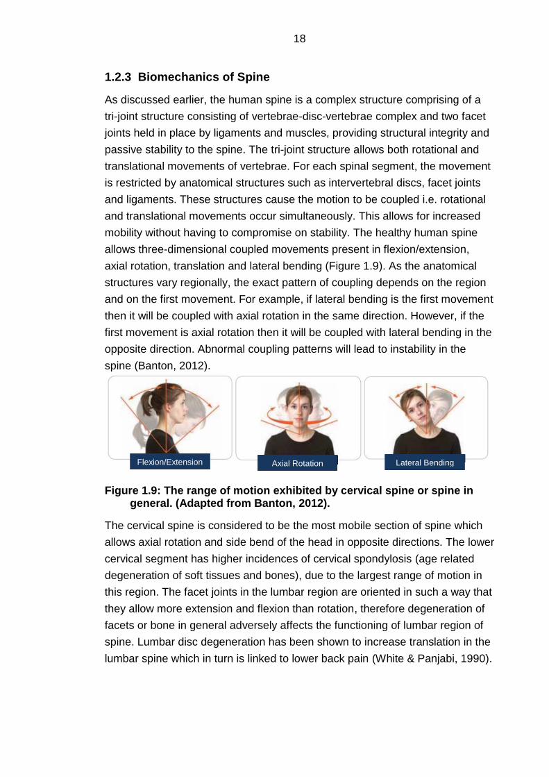
18
1.2.3 Biomechanics of Spine
As discussed earlier, the human spine is a complex structure comprising of a
tri-joint structure consisting of vertebrae-disc-vertebrae complex and two facet
joints held in place by ligaments and muscles, providing structural integrity and
passive stability to the spine. The tri-joint structure allows both rotational and
translational movements of vertebrae. For each spinal segment, the movement
is restricted by anatomical structures such as intervertebral discs, facet joints
and ligaments. These structures cause the motion to be coupled i.e. rotational
and translational movements occur simultaneously. This allows for increased
mobility without having to compromise on stability. The healthy human spine
allows three-dimensional coupled movements present in flexion/extension,
axial rotation, translation and lateral bending (Figure 1.9). As the anatomical
structures vary regionally, the exact pattern of coupling depends on the region
and on the first movement. For example, if lateral bending is the first movement
then it will be coupled with axial rotation in the same direction. However, if the
first movement is axial rotation then it will be coupled with lateral bending in the
opposite direction. Abnormal coupling patterns will lead to instability in the
spine (Banton, 2012).
Figure 1.9: The range of motion exhibited by cervical spine or spine in general. (Adapted from Banton, 2012).
The cervical spine is considered to be the most mobile section of spine which
allows axial rotation and side bend of the head in opposite directions. The lower
cervical segment has higher incidences of cervical spondylosis (age related
degeneration of soft tissues and bones), due to the largest range of motion in
this region. The facet joints in the lumbar region are oriented in such a way that
they allow more extension and flexion than rotation, therefore degeneration of
facets or bone in general adversely affects the functioning of lumbar region of
spine. Lumbar disc degeneration has been shown to increase translation in the
lumbar spine which in turn is linked to lower back pain (White & Panjabi, 1990).
Flexion/Extension Axial Rotation Lateral Bending

19
1.2.4 Biomechanics of Spinal Ligaments
The biomechanical functions of the spine are partly accomplished by the
mechanical behaviour of the individual ligaments. These ligaments have been
shown to provide passive stability to the spine and play a major mechanical
role within the physiological range of motion (Bowden, et al., 2008). The
physical characteristics i.e. the locations and orientations of all the ligaments
have been discussed in detail previously (Section 1.2.1.5). The functional role
of ligaments is described in the following section.
1.2.4.1 Non-Linear Behaviour
The stiffness and strength of the ligaments are important factors in spinal
biomechanics, especially during trauma to the spine. One of the characteristics
of a ligament that helps provide its physiological function is the nonlinearity of
the load-displacement curve. Figure 1.10 shows a typical load-displacement
curve of a spinal ligament (White III & Panjabi, 1990). The curve is divided into
three regions:
I. The neutral zone (NZ) – shows an increase in strain beyond the neutral
position without a corresponding significant increase in stress. This is due
to the uncoiling of the crimp pattern of the collagen fibres which stretches
until the fibres reach a straightened condition.
II. The elastic zone (EZ) – shows a rise in stress with corresponding strain,
stretching the collagen fibres further, beyond the NZ and up to the
physiological limit. This elastic zone is divided into two regions: (i) a non-
linear active zone where the stress starts to increase significantly with the
corresponding strain, and, (ii) an active linear zone where the stress
increases proportionally to the strain (Dumas, et al., 1987).
III. The plastic zone (PZ) – is the region of increasing trauma whereby a non-
linear rise in stress is evident with corresponding strain, stretching the
fibres beyond the physiological limit and until failure occurs. The fibres are
arranged in a ligament in such a manner that loading on the entire
ligament results in some fibres being loaded more than the others and
hence they begin to fail early under increasing load. The plastic zone
represents this behaviour. Progressive loading of a ligament would
eventually result in complete rupture, corresponding to the failure region
on the graph.
The non-linear active zone of the EZ and the NZ, collectively, are commonly
known as the toe-region, whereas the linear active zone is commonly known as

20
the linear-region (Chazal, et al., 1985; Dumas, et al., 1987; Panjabi, et al.,
1982).
Figure 1.10: A typical load-deformation curve of a ligament illustrating the three regions: the neutral zone (NZ), the elastic zone (EZ) and the plastic zone (PZ). (Adapted from White III & Panjabi, 1990).
Spinal ligaments all follow a similar behaviour, when loaded, to the load-
displacement curve shown in Figure 1.10. White III & Panjabi (1990) plotted
physiological load-displacement curves for the most significant ligaments of
lumbar region using the data from Panjabi et al. (1982) (Figure 1.11). All curves
show non-linearity, characterised by their unique combination of stiffness,
maximum deformation and failure load. The variations in their behaviour are a
reflection of the role of each of the ligaments. Chazal et al. (1985) established a
correlation between stress and strain values for spinal ligaments. It was found
that the ALL exhibited largest deformations for lowest loads while the ITL
exhibited smallest deformation for highest loads. The difference in the
behaviour of the ALL observed between Panjabi et al. (1982) and Chazal et al.
(1985) is due to the difference in testing. Chazal et al. (1985) performed the
testing on ligaments in isolation whereas Panjabi et al. (1982) performed the
testing in-situ, i.e. within a whole functional spinal unit, by applying
physiological loads and moments. Kirby et al. (1989) has shown that the
stiffness of the longitudinal ligaments increases for strain of up to about 0.12,
after that it becomes constant until the signs of failure are visible. The
longitudinal ligaments were found to require higher stress to induce a given
strain, up to a value of 1.5, as compared to the LF. The LF showed no signs of
Load or Stress Failure
Trauma range
Physiological range
NZ EZ PZ
Deformation or strain

21
failure up to a strain value of 1.5. Myklebust et al. (1988) tested individual
ligaments, in situ, in isolation. It was generally concluded that as the distance
from the vertebral centre of rotation is increased, the deflection at failure also
tended to increase because these far ligaments must functionally withstand
more force and deflection.
Figure 1.11: Force deformation curve for spinal ligaments of lumbar region (Adapted from White III & Panjabi, 1990).
1.2.4.2 Viscoelastic Nature
Viscoelastic materials are characterised by both viscous and elastic properties
when undergoing deformation. Because of the viscosity factor they have a time
dependant behaviour even when they are subjected to constant loads. Unlike
elastic materials, when a load is applied to viscoelastic materials and then
removed, some of the energy stored is recovered while the remainder is
dissipated in the form of heat. This dissipation of energy is known as hysteresis
and is defined by the area between the loading and unloading curve (see
Figure 1.12). Chazal et al. (1985) observed all spinal ligaments exhibited
hysteresis during the loading-unloading curve owing to their viscoelastic nature.
When viscoelastic materials like ligaments are loaded and unloaded a few
times in a cyclic manner, the hysteresis, i.e. the energy lost in each respective
cycle, is reduced with each consecutive cycle. An equilibrium, close to zero
energy lost, is usually reached whereby the loading and unloading curves
become repeatable, indicating the importance of preconditioning before
experimental testing. Pre-conditioning reduces the effect of the viscous part of
the material behaviour as it can be dependent on the hydration level of the
material whereas the elastic part is easily characterised and repeatable.
PLL ALL ISL LF CL SSL
LUMBAR
Force (N)
DEFORMATION (mm)

22
Ligaments display time and history dependant viscoelasticity when undergoing
deformation due to the presence of both a viscous proteoglycan gel substance
and elastic collagen fibres and elastin. This means they would provide
increased stiffness with increasing loading rate compared to when the loads
are applied slowly (Hukins, et al., 1990). If kept within the physiological range,
they would retrieve their original shape once the load is removed but the
recovery would take longer than an elastic structure. These are important
characteristics responsible for their shock-absorbing capacity.
Figure 1.12: A comparison of purely elastic (a) and viscoelastic (b) material showing hysteresis presented by the viscoelastic material.
1.2.4.3 Pre-tension/Pre-strain
Connective tissues such as ligaments, tendons and skeletal muscles are
known to retract when excised from the body. This behaviour is attributed to the
in situ strains that exists in vivo in the absence of any loading and is usually
considered as a reference state from which different motions can be simulated.
Removing the tissue from the body yields a relatively stress-free configuration,
relieving the strains and associated stress hence the retracting. This in-situ
strain (i.e. pre-strain) for ligaments has been shown to contribute to the stability
of the joints (Ellis, et al., 2006). Spinal ligaments have also been shown to be
pre-strained in a spine from which all the muscles have been removed. This
behaviour is shown by the retracting of the ligaments when cut (Hukins, et al.,
1990; Tkaczuk, 1968). The ALL and PLL have been shown to have a pre-strain
of up to 10% and 13% respectively (Tkaczuk, 1968) in the parallel fibre
direction and it not only affects their own stress and strain state but the overall
biomechanics of the spine (Hukins, et al., 1990; Nachemson & Evans, 1968;
Tkaczuk, 1968; Petter, 1933). Pre-strain is reported to significantly decrease
with age (Nachemson & Evans, 1968; Tkaczuk, 1968) with the LF shown to
loading
unloading
No energy loss Str
ess
Strain
(a)
loading
unloading
Hysteresis is the energy loss S
tre
ss
Strain
(b)

23
buckle into the spinal canal on physiologic extension (Penning & Wilmink,
1986).
1.2.5 Experimental Testing of Spinal Ligaments
This section provides a review of the experimental testing procedures
previously used to investigate properties of the spinal ligaments. This includes
specimen preparation, mechanical test design and investigation of
microstructures. Two distinct methods of testing have been cited in literature:
individual ligament testing and whole functional spinal unit testing. This section
of the literature review discusses the two methods and highlights the
procedures along with their merits and demerits. The various studies have
different loading techniques, rates, and magnitudes which provide a great deal
of information but is challenging for comparison purposes. The values of the
mechanical properties of the ligaments obtained as a result of both methods of
testing are presented in tabular form at the end of this section (Tables 1.2 to
1.8).
1.2.5.1 Individual Ligament Testing
Studies by Tkaczuk (1968), Nachemson & Evans (1968), Waters & Morris
(1973), Chazal et al. (1985) and Kirby et al. (1988) have all focused on
experimental biomechanical characterisation of individual ligaments. These
studies have all used various techniques and testing protocols to extract and
load ligaments. An extensive amount of data has been accumulated, however,
comparison of data obtained as a result of these various studies shows
considerable differences in the values obtained.
1.2.5.1.1 Specimen Preparation, Fixation and Maintenance
Storage
The method of storage of connective tissue could bring about changes in its
mechanical properties (Waters & Morris, 1973) hence it is an important
consideration during the planning of an experiment. There are a number of
different methods used by researchers for storage of ligaments in
biomechanical investigations including: testing fresh, freezing and storage at
room temperature or refrigerator, in sealed bags or in a fluid. The methods
used will be described in more detail in the following paragraphs.
Tkaczuk (1968) and Nachemson & Evans (1968) both obtained specimens
from fresh cadavers and tested them either on the day of autopsy or within 48
hours of retrieval. Wherever delayed, Nachemson & Evans (1968) stored the
samples at -29ºC, in sealed plastic bags, and used within 3 days. Kirby et al.

24
(1988) froze the specimens, obtained from frozen pigs, immediately in liquid
nitrogen (-196 ºC) and stored in a deep freezer at (-20 ºC). Waters & Morris
(1973) stored the specimens at 10ºC in watertight plastic bags, to maintain
constant hydration without the use of humidity chamber, and tested within 48
hours of retrieval. Chazal et al. (1985) also maintained proper hydration by
keeping the ligaments obtained from fresh cadavers or living subjects in a
solution of water, alcohol and glycerine when the testing was delayed for few
hours or the ligaments were placed in Ringer’s solution when tested within one
hour. The authors did not make any comparison between the two methods.
Nachemson & Evans (1968) showed that this method of storing ligaments (LF)
in immersed conditions even for an hour increases the weight of tissue by 7-
10%. This will also have an effect on the respective geometric properties of the
tissues.
Water content in the tissue is generally attributed to cause artefacts due to the
freezing process. Volumetric changes of 6.2% for human muscle tissue were
reported by Pech et al. (1987) (Pech, et al., 1987). However, the muscle tissue
has much higher water content than the ligament therefore as long as such
connective tissues are frozen at sufficiently low temperatures; their tensile
properties appear to remain unaffected (Mathews & Ellis, 1968; Nordwall,
1973). Viidik et al. (1965) used sealed containers to store rabbit ligaments at
20ºC for 96 hours and found the collagen bundles to still be preserved for this
time period. Although the collagen fibre bundles were found to be swollen at 2
hours with autolysis of cell nuclei beginning at 24 hours and completing at 96
hours, the tensile characteristics of the ligaments were found to be unaltered
until after 96 hours. Specifically for spinal ligaments, Tkaczuk (1968) has found
that rapid freezing to -60ºC and thawing of ALL & PLL does not have any effect
on the mechanical properties of tissue samples. Hickey & Hukins (1979) also
demonstrated that freezing does not have any effect on the orientation of the
collagen fibrils in connective tissues.
None of the storage temperatures discussed above were shown to cause any
adverse effect on the structure or state of the specimens. These studies show
that specimens can either be tested on the day of retrieval or within 48 hours by
keeping them moist and storing in refrigerator or, if need be, the specimens can
be frozen on the day of retrieval and then tested on a later date. However,
storing in a fluid will cause the tissue to swell and will affect the corresponding
geometric properties; therefore tissue should be stored in airtight bags to avoid
it drying out.

25
Specimen Geometry
Being able to measure the geometry of ligaments (length and cross sectional
area) accurately is an important consideration for planning the tests to work out
the mechanical properties of ligaments. An error in the cross-sectional area
measurement has been cited as the single greatest source of technical error in
this type of experiments (Waters & Morris, 1973). The method of measurement
has to be accurate to detect possible small differences in mechanical properties
of different ligaments or sections of ligaments. Various methods of determining
the geometric parameters of the ligaments have been used in literature
including: direct measurement using displacement gauges, microtomes or
palpators and indirect measurement using masses and densities or graphic
methods.
In terms of direct measurement, Tkaczuk (1968), Nachemsom & Evans (1968)
and Chazal et al. (1985) all used measuring instruments for determining the
length and cross-sectional area of ligaments. Tkaczuk (1968) tested whole
individual ligaments as well as samples of identical sizes. The samples of ALL
and PLL were cut into segments and subsequently frozen to allow cutting
sheets of 0.5 mm thickness using a freezing microtome. A dial displacement
gauge was used to measure the thickness of samples whereby the sample was
placed between two metal plates. The 0.5 mm thick sheets were then used to
obtain identical samples of uniform width of 2 mm, this was achieved by using
pressing stamp method to stamp a soft plastic material placed under the sheet
and subsequently cutting the ligaments parallel to the orientation of the
collagen fibres. The dial displacement gauge and the pressing stamp method
appeared to be a good way of obtaining specimens of identical sizes.
Nachemson & Evans (1968) tested LF attached to their laminae with the
vertebral bodies and articular processes removed. The dimensions were
measured using a micrometre and callipers. This method of measuring
dimensions may not be accurate because the specimen might be deformed by
the micrometer during measurement. The authors did not mention if they took
measurements at one position or at many locations to take an average to avoid
the inaccuracy in values obtained due to the inhomogeneity in ligament
structure over the entire length.
Chazal et al. (1985) also conducted a study on the LF with bony attachments at
each side to include both the short and long fibres in order to gain accurate
mechanical properties, dependant on anatomical integrity of the ligament. A
palpator was used to measure cross section of ligaments every 2 mm on the
entire length with the tracing being obtained on a graph paper using an

26
amplifier. The lowest cross-section was used to calculate stress. The length
was measured at rest using a micrometer, however, since the length was
measured at rest in isolation it would not be a true representation of the actual
length of ligament under its normal state of pre-tension in situ.
Several groups used a variety of indirect methods for measuring the
dimensions of ligaments including Water & Morris (1973) and Kirby et al.
(1989). Waters & Morris (1973) obtained the cross sectional areas of the
specimens by first clamping the ligament under slight tension and freezing it
rapidly with liquid nitrogen. The ligaments were then sectioned in 2 mm
segments and were allowed to thaw under a concave coverslip that prevented
water loss without touching the specimen. The specimen was then placed on a
projector, a thin cross section of ligament was magnified and projected on a
screen, and the area of the magnified image was determined by a graphical
method. This method provides a simple approach however it does not take into
account the variability in the thickness of ligaments across the entire length.
Kirby et al. (1989) determined the cross-sectional areas from masses and
densities of the specimens by mixing carbon tetra-chloride and xylene to
produce a liquid in which they neither floated nor sank (Sikoryn & Hukins,
1988). This method relies heavily on getting the consistency of the mixture
accurate each time and also the pre-tension in ligaments is not accounted for.
In summary, various methods of measuring the length and cross sectional
areas of the ligaments have been established, however, each method has its
own shortcoming as described above. The ideal method would incorporate both
the pre-tension in the ligaments to obtain accurate length and the variability in
the cross-section of ligaments through their entire length.
Fixation
Tkaczuk (1968) and Kirby et al. (1989) tested ligaments individually without any
bony attachments by firmly attaching a clamp to the ends of the ligaments.
Chazal et al. (1985), Nachemson & Evans (1968) and Waters & Morris (1973)
clamped the bones, attached to ligaments to preserve their anatomical and
mechanical integrity. The method of testing ligaments attached to their bones is
better due to its ease of fixation and also because it avoids the damage to the
structure of ligament due to clamping. However, when only sections of
ligaments are to be tested, it is not possible to have bones on either end and
hence the use of specialised holders is recommended which would minimise
the effects of slipage and surface damage.

27
Test Environment
The physical properties of connective tissues can be greatly affected by their
state of hydration (Waters & Morris, 1973). Stromberg and Wiederheilm (1969)
found the mouse tail tendon dried rapidly when exposed to room temperature
with shrinkage and shortening within seconds of exposure. Tkaczuk (1968) also
observed similar patterns during testing of ALL and PLL from fresh cadavers.
He noted drying of specimens at room air of 60-70% humidity while excessive
uptake of water by the specimens when tested in Ringer’s or other solutions.
The tests were performed in high humidity chamber (100%) to prevent water
loss from the tissues that can affect their physical properties. Waters & Morris
(1973) performed the tests in a heat-sealed tubular plastic sleeve at either end
to maintain constant hydration. Nachemson & Evans (1968) performed tests on
samples immersed in Ringer’s solution hence the stress-strain values obtained
were thought to be slightly inaccurate due to small changes in dimensions by
the swelling of tissue, however, the results were used only for comparison
within the study. Kirby et al. (1989) decided to conduct the tests at room
temperature by constantly spraying the specimens with saline; to avoid drying
off of the specimens. Studies on some ligaments have shown the stress-strain
curves at 20ºC and at body temperature to be indistinguishable (Dorlot, et al.,
1980) (Hasberry & Pearcy, 1986).
From above, it can be concluded that the tissue should be kept moist
throughout the procedure but it must not be placed in a solution otherwise it
would swell and exhibit inaccurate mechanical properties, and that testing at
room temperate is acceptable.
1.2.5.1.2 Test Design and Loading Regime
Preliminary or Calibration Tests
Various authors (Tkaczuk, 1968; Waters & Morris, 1973) have undertaken
initial tests to determine the most appropriate loading regime e.g. by testing
initial specimens to failure (tearing of ligament) to check maximum loads that
should be applied in subsequent experiments. Tkaczuk (1968) suggested using
maximum loads of about 30% of the failure load of weakest sample used. This
is useful as structures do not return to their original state after they have gone
past their elastic limit therefore it is crucial to test them well within the elastic
range if further tests are to be undertaken.

28
Actual Tests
A displacement control was mostly used by researchers to test the ligaments.
Nachemson & Evan (1968) conducted tests on LF at a constant strain rate of
0.0055 s-1 which is of the same order as the strain rate of 0.003s-1 used by
Kirby et al. (1989) to test both the LF and the longitudinal ligaments. Chazal et
al. (1985) also used a slow constant rate of 1mm/min (~0.017 mm/s) to test the
specimens in tension. Since multiple ligament types from various levels of
spines were tested in these studies, the lengths (hence strains) will be very
different, so it is hard to make meaningful comparisons. It has been shown
previously that the loading rate has a significant effect on the stiffness such that
stiffness increased linearly with the logarithm of the loading rate (Yoganandan,
et al., 1989). Moreover, increased loading rate has been shown to shorten the
toe region, increase stress and reduce failure elongation (Shim, et al., 2005).
Therefore loading rate of the test should be selected to replicate the loading
rate of interest in vivo. Furthermore, different ligaments of the spinal motion
segment tend to undergo different amounts of strain in different motions. For
example, the PLL has been shown to have a physiological maximum strain of
about 13% in extension whereas SSL has been found to have maximum strain
of about 31% in the same motion (Panjabi, et al., 1982). Therefore, it is not
surprising that different strain rates have been used depending on the type of
motion under consideration and the type of ligament under test. However, the
strain rates used by Kirby et al. (1989) and Nachemson & Evan (1968) appear
low for physiological movement, for example, at a strain rate of 0.003 s-1
ligament would take over 40 seconds to reach a physiological stretch of 13%.
Preloading (Tkaczuk, 1968) or resting-stress (Nachemson & Morris, 1964)
values were also determined. Nachemson & Evan (1968) determined the
resting stress from the contractional strain that occurred when the vertebral
arches were separated from vertebral bodies. In both studies, the resting strain
was found to be dependent on the IVD condition and on the condition of spine
in general. It was found that the results varied markedly across samples since
pre-stress values are dependent on dimensions of the ligaments, the pressures
within the nucleus pulposus and the elasticity of annulus fibrosus.
The effect of repeated loading was also determined by Tkaczuk (1968) and
Nachemson & Evan (1968) by cyclically loading all the samples. Tkaczuk
(1968) performed three loading cycles on both ALL and PLL specimens and
found significant differences between the parameters obtained from both the
ligaments although these differences were found to decrease in the 2nd and 3rd
load cycles. Moreover, similar proportional change of mean parameters was

29
found between each load cycle for both the ligaments. Nachemson & Evan
(1968) established that LF deforms elastically over much of its deformation
range; owing to the elastin fibres which account for approximately 65% of its
dry weight, and that the time-dependant properties of ligament increase in
magnitude with increase in stress but are negligible at very low stresses.
Nachemson & Evan (1968) also demonstrated that strains of less than 30-60%
on the LF were fully recoverable on removal of the stress.
1.2.5.2 In-situ Ligament Testing
Panjabi et al. (1982), Dumas et al. (1987), Myklebust et al. (1988), and Heuer
et al. (2007) all tested ligaments in situ, intact with the spinal canal or the
functional spinal unit. The studies analysed the changes in the range of motion
of the spinal segments, by sequentially cutting the ligaments, in order to assess
the role of each ligament in spine kinematics. These studies, just like those in
the previous section, have their merits and shortcomings which are discussed
in the following section.
1.2.5.2.1 Specimen Preparation, Fixation and Maintenance
Storage
The storage methods used by the aforementioned studies on in situ ligament
testing are quite similar to the ones used in individual ligaments testing. Dumas
et al. (1987) left some muscle tissue on the specimens during preparation,
before storage, in order to keep the ligaments moist by protecting the contact
with the air. Pintar et al. (1992) froze specimens in the intact state with
sandbags placed in appropriate position to maintain normal spinal curvature.
Specimen Type
There are two types of specimens used in such in situ ligament testing studies:
I. A whole functional spinal unit with all the ligaments intact, transecting
ligaments in turn until only the bones and discs remain.
II. Individual ligaments, in situ, in isolation i.e. removing all other ligaments,
disc and supporting structures from the vertebral body except the one
under study.
Dumas et al. (1987), Panjabi et al. (1982) and Heuer et al. (2007) all used the
first type of specimen in order to test either the biomechanical behaviour of
ligaments (Panjabi, et al., 1982; Dumas, et al., 1987) or to study the
biomechanical effect of stepwise anatomy reduction for various loading
directions and magnitudes (Heuer, et al., 2007).

30
Myklebust et al. (1988) used the second type of specimen to test ALL, PLL,
both joint capsule (JC), ISL and LF at each spinal level from C2-S1. The SSL
was also evaluated but only in the lumbar and thoracic regions. The fibres of
the ALL and PLL are normally interwoven with the disc and it is difficult to draw
a clear boundary between these longitudinal ligaments and the disc. The
investigators solved this issue by differentiating the fibres based on their
orientation. The ones belonging to the ligament were noted to be vertical while
the ones of the disc were found to be oblique. Similarly, the testing of JCL is
impossible without keeping the facet joints intact; therefore, the JCs were
tested as a bilateral unit, comprising of both the JCLs and the facet joints. The
LF was distinguished from the ISL due to its characteristic yellow colour while
the SSL was differentiated from the ISL by defining the end of spinous process
to be the division between the two.
Pintar et al. (1992) also used the second type of specimen to test ligaments.
They focussed on keeping the proper alignment of the spinal column. The
specimens were frozen and marked under computed tomography (CT) to
maintain alignment and photographed to obtain the dimensions.
Fixation
These in situ studies face fewer issues in terms of fixation as it is easier to fix
hard structures i.e. bones in the testing apparatus than soft tissue structures
such a ligaments which are prone to slippage and deformation/damage from
the site of fixation. The general approach followed in these studies was to fix
one vertebra, usually the bottom one and attach the loading frame or testing rig
to the top vertebrae and apply different types of forces/moments to it. Panjabi
et al. (1982) and Myklebust et al. (1988) rigidly fixed the vertebral bodies
attached to the top and bottom of ligament under consideration, as illustrated in
Figure 1.13. Others have used potting methods to hold the vertebrae in place.
Dumas et al. (1987) employed cylindrical metal cups with three screws to hold
vertebrae in place before pouring fast setting epoxy resin (Figure 1.14). Metal
guides were used to assure parallelism of cups. Heuer et al. (2007) embedded
the FSU in PMMA from both sides with radio-translucent screws placed in the
vertebrae prior to potting to provide better fixation. The potting method has
advantages over the direct attachment to the testing machine as several
specimens can be pre-prepared using the pots and stored in the
refrigerator/freezer and tested one after another, saving time spent on
preparation and potting in between tests.

31
Figure 1.13: Schematic representation of specimen fixation (Adapted from Myklebust, et al., 1988)
Figure 1.14: Photograph of the FSU in the metal cup (Adapted from Dumas, et al., 1987)
Test Environment
Dissection for in-situ ligament testing was performed at room temperature in
90-100% humidity chamber (Panjabi, et al., 1982; Dumas, et al., 1987) or using
Ringers solution (Myklebust, et al., 1988). After dissection, Dumas et al. (1987)
kept the ligaments covered until the testing with a commercial jelly, Lubafax, in
order to prevent dehydration. Heuer et al. (2007) used a different approach to
other studies and kept the specimens moist by wrapping them with 0.9% saline
gauzes throughout the entire testing. This is a more practical way of keeping
the tissue moist because testing within a high humidity chamber requires
specialised equipment or a chamber to be built. Also working in high humidity
chambers would be difficult for manipulating the specimens into the testing
apparatus.
1.2.5.2.2 Mechanical Test Design
Preliminary or Calibration Tests
Dumas et al. (1987) performed preliminary tests to measure the stiffness of
resin used to fix the vertebrae into the metal cups. The resin was found to have

32
higher stiffness by an order of magnitude than the ligaments stiffness.
Therefore its deformation was considered to be negligible compared to
ligament deformation for testing. The maximum loads used in the experiments
were predetermined so that no permanent damage to the ligaments could
occur. The investigators also determined the order of resecting the ligaments to
choose the one which gave well separated curves, i.e. where the ligament with
the most effect is cut first in order to avoid overriding the effects of other
ligaments. This order was found to be from anterior to posterior. In order to
reduce the water content of the specimens, Heuer et al. (2007) exposed the
specimens to 500 N axial compression for 15 minutes.
Actual Tests/ Measurements Taken
Panjabi et al. (1982) conducted a study to determine physiological strains in
each of the lumbar spinal ligaments during spine movement in three
dimensions. They applied 12 different types of physiological loads at the
geometric centre of the upper vertebral body and measured the deflection of
this vertebra under load. The locations of the spinal ligaments for the neutral
position of the FSU were determined by measuring the coordinates of various
ligament attachment points. The flexion extension curves (on motion versus
moment plots) were found to not meet each other at the origin, implying that
there exists a zone for the neutral position of spine. The spine can lie anywhere
within this zone on the application of smaller loads. This zone was named as
the “neutral zone (NZ)”. To move the spine outside the neutral zone, higher
loads were required. These regions of increasing resistance, both on the
negative and positive side of neutral zone, were termed as active zones. This
increasing resistance to motion involves the elastic deformation of the soft
tissues produced by the activation of muscles. In degenerated specimens the
neutral zones were found to be generally wider indicating a higher probability of
over-stretching the ligaments in a degenerated state.
Myklebust et al. (1988) used an M.T.S. (Minneapolis, MN) electrohydraulic
system to apply direct axial tension to the specimens at 10 mm/s and obtained
force versus deflection curves. Failure loads alongside failure deflections were
also obtained. A similar method of measuring the displacement to Panjabi, et
al. (1982) was used. Pintar et al. (1992) used the same testing procedure in
order to determine the mechanical properties of spinal ligaments for direct
incorporation into mathematical or finite element model.
Dumas et al. (1987) and Heuer et al. (2007) both performed preconditioning on
the ligaments by submitting the specimens to several loading cycles in order to
make the final response repeatable (see Section 1.2.4.2) hence minimising the

33
effect of viscoelasticity by capturing the reproducible elastic behaviour in the
ligament. Preconditioning of the ligaments is important as it removes any
crimping in the ligaments as a result of being stored in a frozen and fixed
position by returning the structural collagen fibres to proper physiological
conditions (Hashemi, et al., 2005). This results in a response that is repeatable
and a better representative of normal physiological response (Van Ee et al.,
2000). The last loading cycle was recorded to collect data for evaluation.
Subsequently the specimens were reduced in structures by transecting the
ligaments in turn. This way, a set of curves were obtained for each specimen.
In order to compare the curves across different specimens, Dumas et al. (1987)
calculated force at the linearity point i.e. the point where non-linear curve and
linear curve differ significantly, and the rigidity which is defined as the slope of
the linear portion of the curve (K).
Dumas et al. (1987) and Heuer et al. (2007), both, also measured the pre-
tension exerted by the ligaments. Dumas et al. (1987) used a conventional
method of resecting the ligaments and noting the force created as the pre-
tension exerted by the ligaments. Whereas, Heuer et al. (2007) established
pre-tension by introducing a concept of lordosis angle (the angle at the
unloaded posture).
1.2.5.3 Mechanical Properties of Ligaments from Experimental Studies
The following section lays out the spread of experimental data on various
aspects of lumbar spinal ligaments properties. The results are tabulated for
comparison purposes both amongst the studies and with the result of the
current study.

34
Table 1.2: Mechanical properties of anterior longitudinal ligament (ALL).
Author
Mechanical Properties
Pre-strain (%)
Pre-loading
(N)
Failure Strain (%)
Failure stress
(N/mm2)
Failure Load (N)
Failure Deflection
(mm)
Mean strain at limits of
NZ (%)
Maximum Strain (%)
Stiffness (N/mm)
Tkaczuk (1968)1 10.9 1.77 20.8 330
Panjabi et al. (1984) 6
Chazal et al.
(1985)2
28 10.6 437 25 12.85 (extension)
Myklebust et al. (1988)
209±196 –
676±359
11.5±12.1 –
20.4±3.5
Pintar et al. (1992) 28.1±18.3 –
49±31.7
8.2±2.5 –
16.1±6.2
33±15.7
Notes:
1Tkaczuk et al. (1968):
ALL shortened less than PLL on removal.
Degenerative changes in disc shown to effect the subsequent shortening of ligament.
Exact pre-stress in a ligament was difficult to determine as it depended on the dimensions of ligaments and the pressure within nucleus pulposus and on the elasticity of annulus fibrosus.
2 Chazal et al. (1985):
Stress and strain at linearity point (start of linear region) on the load-deformation curve were reported as 1.15 N/mm2 and 25% respectively.
Stress and strain at plasticity point (end of linear region) on the load-deformation curve were reported as 9.11 N/mm2 and 18.1% respectively.

35
Table 1.3: Mechanical properties of posterior longitudinal ligament (PLL)
Author
Mechanical Properties
Pre-strain (%)
Pre-loading
(N)
Failure strain (%)
Failure stress
(N/mm2)
Failure Load (N)
Failure Deflection
(mm)
Mean strain at limits of
NZ (%)
Maximum Strain (%)
Stiffness (N/mm)
Tkaczuk (1968) 13.4 2.94 19.42
Panjabi et al. (1984)
5.75
Chazal et al. (1985)1
29.5 20.8 45 13.5 (flexion)
Myklebust et al. (1988)
38±15 –
160±82
4.2±0.1 –
7±3.2
Pintar et al. (1992)
11.3±0.2 –
16.2±9.3
7.2±4.1 –
28.4±11.3
20.4±11.9
Notes: 1Chazal et al. (1985)
Stress and strain at linearity point (start of linear region) on the load-deformation curve were reported as 2.04 N/mm2 and 45% respectively.
Stress and strain at plasticity point (end of linear region) on the load-deformation curve were reported as 16.2 N/mm2 and 0.34% respectively.

36
Table 1.4: Mechanical properties of ligamentum flavum (LF)
Author
Mechanical Properties
Modulus of Elasticity (N/mm2)
Force at linearity
point (N)
Failure Strain (%)
Failure Stress
(N/mm2)
Failure Load (N)
Failure Deflection
(mm)
Mean strain at limits of
NZ (%)
Maximum Strain (%)
Stiffness/K (N/mm)
Nachemson & Evan (1968)1
19.6(elderly) –
98(young)
277* 30(elderly) –
70(young)
1.96(elderly) –
9.8(young)
315 16.20 (flexion)
133 (old) –
665(young)*
Panjabi et al. (1984) 150 – 200*
7.1 & 7.2 310*
Chazal et al. (1985)2 19 15.2 16.6
Dumas et al. (1987) 170 358
Myklebust (1988) 133±41 –
334±158
4.5±1.3 –
14.5±3.4
Pintar et al. (1992) 28.8±8.2 –
102±2.9
1.3±0.4 –
4.1±0.5
27.2±9.2
Notes:
*Values were estimated by Dumas et al. (1987) 1Nachmenson & Evans (1968)
Tests conducted at a constant strain rate of 0.33/min.
LF remained elastic in the physiological stress range; strains of 30-60% were found to be fully recoverable on removal of stress.
Stress relaxation tests showed that the LF does behave in a non-linear viscoelastic manner although its time-dependent behaviour is not much significant at very low stresses but increase in magnitude with increasing stress.
Found to pre-stress disc by a force ranging from 1.5kg in young to 0.4kg in old causing intradiscal pressures of 0.7kg/cm2. 2Chazal et al. (1985)
Stress and strain at linearity point (start of linear region) on the load-deformation curve were reported as 3.17N/mm2 and 16.6% respectively.
Stress and strain at plasticity point (end of linear region) on the load-deformation curve were reported as 13.57N/mm2 and 18.7% respectively.

37
Table 1.5: Mechanical properties of intertransverse ligament (ITL)
Author
Mechanical Properties
Failure Strain (%)
Failure Stress (N/mm2)
Mean strain at limits of NZ (%)
Maximum Strain (%)
Panjabi et al. (1984)1 13.5 25.50 in lateral bending
Chazal et al. (1985) 4.2 51 8.2
Notes:
1Panjabi et al. (1984)
Stress and strain at linearity point (start of linear region) on the load-deformation curve were reported as 10.85N/mm2 and 8.2% respectively.
Stress and strain at plasticity point (end of linear region) on the load-deformation curve were reported as 47N/mm2 and 0.15 respectively.
ITL was found to have highest mean stress value with lowest mean strain value amongst other ligaments, showing its high resistance.

38
Table 1.6: Mechanical properties of interspinous ligament (ISL)
Author
Mechanical Properties
Force at linearity
point (N)
Failure Strain (%)
Failure Stress
(N/mm2)
Failure Load (N)
Failure Deflection
(mm)
Mean Strain at
limits of NZ (%)
Maximum Strain (%)
Stiffness/K (N/mm)
Waters & Morris (1973) 341* 18-34 1530*
1Chazal et al. (1985) (tested ISL with SSL)
38.5 8.71 80-300 41.6
Myklebust et al. (1988) 95±22 –
185±41
7.4±3.3 –
17.8±0.6
Panjabi et al. (1984) 50-100* 10.9 27.90 (flexion)
218*
Pintar et.al (1992) 51.5±2.9 –
119.7±14.7
1.8±0.1 –
5.9±1.8
11.5±6.6
*Dumas et al. (1987) 82 80 Notes: *Values were estimated by Dumas et al. (1987)
1Chazal et al. (1985)
Stress and strain at linearity point (start of linear region) on the load-deformation curve were reported as 1.75N/mm2 and 41.6% respectively
Stress and strain at plasticity point (end of linear region) on the load-deformation curve were reported as 7.92N/mm2 and 30.5% respectively

39
Table 1.7: Mechanical properties of supraspinous ligament (SSL)
Author
Mechanical Properties
Force at linearity
point (N)
Failure Strain (%)
Failure Stress
(N/mm2)
Failure Load (N)
Failure Deflection
(N)
Maximum Strain (%)
Stiffness/K (N/mm)
Panjabi et al. (1984) 50-100* 31.95 (flexion) 100*
*Dumas et al. (1987) 66 75
Myklebust et al. (1988) 226 – 750±159 21.1 – 29.2
Pintar et al. (1992) 70.6 ± 45 –
115.1 ± 49.1
8.9±3.2 –
15.5±5.1
23.7±10.9
Note: *Values were estimated by Dumas et al. (1987)
Table 1.8: Mechanical properties of joint capsular ligament (JCL)
Author
Mechanical Properties
Failure Strain (%)
Failure Stress (N/mm2)
Failure Load (N)
Failure Deflection
(mm)
Maximum Strain (%)
Stiffness (N/mm)
*Panjabi et al. (1984) 19.25 (rotation)
Myklebust et al. (1988)
252±22 –
429±122
9.8±1.6 –
12.8±2.5
Pintar et al. (1992) 47.9±5.4 – 90.4±17.7 3.5±1.2 – 4.4±1.4 33.9±10.7
Notes:
*Panjabi et al. (1984)
Only ligament that was found to resist axial rotation.
When the CL on one side was stretched the one on the other side was found to be shortened.

40
1.2.5.4 Discussion
The above mentioned studies all give considerable amount of data on
biomechanical parameters and mechanical properties of ligaments, however
the results are quite varied. Although the geometric parameters were calculated
and presented, there is huge amount of variability across studies due to
differences in the measurement procedures, for the individual ligament testing
studies. Based on these results, it is difficult to determine which method is the
most accurate for measuring geometric properties. Although dissection is never
raised as an issue in any of the aforementioned studies, it is one of the most
challenging parts of mechanical testing of individual ligaments. The ligaments
do not follow the same pattern within a specimen or across different
specimens. The fibres run in all directions and interweave with fibres of other
tissues, such as the discs, making the distinction between the two difficult.
They also tend to have different width and thickness across the entire length
making it even harder to predict their boundary for accurate dissection of the
entire structure. The removal of ligaments from the spinal column for testing
often results in damage to the ligament. Pre-tension in the ligament is another
important consideration which is often neglected in most of the studies apart
from Tkaczuk (1968). When the ligaments are removed for individual testing,
they lose the constant pre-tension they are under, in the intact state, in the
spine. Hence, the stress-strain curves derived would start at a different point to
that if a pre-strain were applied first. This makes it harder to compare between
studies. Another disadvantage of individual ligament testing is the difficulty of
fixation, the ligaments either have to be removed with the bony attachments or
specialised clamping systems have to be employed to avoid slippage of the
specimen and damage of the specimen from the areas of contact in the clamp.
The technique is also unable to define the role of ligaments in relation to other
spinal components. Despite all its disadvantages, the technique still has an
advantage of being able to produce individual load-displacement curves for
each ligament and is useful when one wants to study the internal structure of
ligaments.
The in situ ligament testing method resolves most of the difficulties stated
above. As the ligaments were tested in the anatomical position in relation to
other structures, their geometry was not needed to obtain the overall
mechanical parameters (e.g. stiffness and strength) hence avoiding the issues
of inaccurate measure of length and cross-sectional area. The challenge of
dissection and extraction of the ligament without damaging its fibres was also

41
avoided by keeping them intact and transecting in steps, when needed.
Keeping the ligaments in situ, in the intact state, will keep them in a more
normal state hence the results better reflect the true behaviour. The problem of
fixation is also resolved at it is easier to fix the vertebrae in the testing
apparatus without the need for designing specialised clamping systems for
each ligament.
The studies reviewed in this chapter have highlighted some useful pointers for
future in situ testing of ligaments, summarised as follows:
The ligaments can be stored in sealed plastic bags at -20°C to -30°C after
retrieval and used later without experiencing any change in their
behaviour.
The tissue can be thawed in a refrigerator rather than at room temperature
and kept moist during testing with saline gauzes to prevent it from drying
out.
The transection can use the distinction between the fibres and orientation
of interconnected ligaments.
The order of the transection of ligaments should be considered as it is
shown to affect the behaviour of ligaments and hence the properties
obtained. In a particular motion, if the ligaments which are higher
contributors to the whole ligament complex behaviour in the FSU are
saved until the end, then the behaviour of all other ligaments will be
dominated by their presence and the resulting stress-strain curves will be
superimposed until those dominating ligaments are transected.
The specimen can be kept in place by holding it between screws in the
pot before pouring in the potting material.
Preconditioning should be considered in order to minimise the effect of
viscoelastic response.
The stiffness of the surrounding materials and holders should be checked
to make sure their deformation would be negligible compared to ligament
deformation for testing.
The maximum loads that will be used in the actual experiments should be
predetermined so that no permanent damage to the ligaments could occur
during testing.

42
All the advantages discussed above makes in situ ligament testing a better
method of evaluating the mechanical properties of spinal ligaments and hence
will be the method of choice of experimental testing for this study. All the points
raised above will be useful considerations when developing the protocol for the
actual study plan. The only disadvantage of in situ ligament testing is to decide
on the motions and devise methods of creating the movements and controlling
them. All the in situ studies above described the role of each ligament in
relation to other structures and gathered substantial amount of data, however,
its comparison and validity is hard to establish as all the studies used different
methods.
1.2.6 Finite Element Modelling of Ligaments
1.2.6.1 Introduction
As discussed in the previous section, a number of studies have been
performed to establish the physical and biomechanical properties of ligaments.
The large variability in outcomes mean that either a large number of
experimental studies have to be performed to gather the full behaviour of each
ligament in the functional spinal unit model or other avenues must be explored.
Computational modelling, using finite element (FE) methods makes it possible
to simulate the complex behaviour of the FSU. Such models can include
detailed representations of the bone and soft tissue structures and their non-
linear material properties. Physical and mechanical properties of ligaments are
required to be able to represent these tissues in the models. The ligaments
have been represented in these models using a number of different types of
finite elements, with different geometries, material properties and initial
conditions.
As discussed above, to develop material models of ligaments, detailed
experimental measurements of the material structure and mechanical
behaviour are needed. The various experimental studies performed on isolated
ligaments as well as in situ ligaments generated useful data describing the
mechanical behaviour of ligaments (Section 1.2.5) and have been used by
researchers to develop FE models of ligaments or of spine in general. Based
on these experimental studies, ligaments have been described as
inhomogeneous, non-linear, anisotropic and viscoelastic structures that
undergo large deformations during elongation (Weiss & Gardiner, 2001). They
have been shown to exhibit a non-linear load-displacement (stress-strain)
behaviour (Section 1.2.4.1) with a neutral zone (NZ), elastic zone (EZ) and
plastic zone (PZ). For the accurate representation of ligaments this non-linear
behaviour must be taken into account in the FE model. In addition, their contact

43
with other tissues and in-situ pre-tension makes the accurate modelling of the
mechanical behaviour of ligaments a challenging task. But these types of
models can also potentially be used to derive the properties (i.e. by reverse
engineering) in a more reliable way than the methods reported in Section 1.2.5
where the ligaments had to be either extracted out or assumptions had to be
made about the geometry.
The following section reviews the literature on a selection of recent finite
element studies that incorporate the spinal ligaments in models. Their
application of in-vitro experimental values such as Young’s modulus, width,
thickness and pre-tension and their choices of finite element type, material
model and attachment sites are explored.
1.2.6.2 Geometry, Material Properties and Material Model
The quantitative information on geometry and material properties of the human
lumbar ligaments, used in FE studies, comes primarily from a limited number of
experimental studies (Tkaczuk, 1968; Chazal, et al., 1985; Pintar, et al., 1992).
The raw data obtained by these primary experimental studies for each of the
spinal ligaments is tabulated in the previous section (Tables 1.2 to 1.8). The
majority of FE studies have used the average value of Young’s modulus for
each of the ligaments while a limited number have used values towards the
lower and upper extremes of the experimental range (Table 1.9). A Poisson’s
ratio of 0.3 has been almost universally chosen for all of the ligaments without
much justification of the choice.
The in-vitro studies mentioned in Section 1.2.5 were mainly focussed on the
material properties of the ligaments. However, most have also recorded
information on the ligament geometry as the material properties have primarily
been derived from the geometry. As discussed previously, the methods used to
determine the geometry have varied and the values obtained are quite different
from each other. Although finite element studies require these dimensions to be
translated into their investigations, the geometric values used are not reported
consistently. For example, Lee & Teo (2005) report only the elastic modulus and
not the cross-sectional area in their study, so it is not possible to derive the
ligament stiffness to make comparisons with the values reported by the in-vitro
studies such as Pintar et al. (1992).
The material properties and cross-sectional area (CSA) used by different
researchers are compared in Table 1.9. As can be seen from the table, the
properties used are quite varied and cross sectional area is not given in all
cases. Some studies did not publish any material property data used. As an
example, the variation in the stress-strain behaviour of the PLL used by

44
different groups is shown in Figure 1.15 using the information summarised in
Table 1.9. The graph clearly shows the variability in model behaviour.
Furthermore, a variety of material models have been used to represent the
ligament behaviour including elastic, viscoelastic and hyperelastic models. The
use of an elastic model by researchers is due partly to the relative insensitivity
of ligaments material behaviour to strain rate over several orders of variations
(Fung, 1993) and partly to the “preconditioned” state that the tissue reach after
repeated loading with minimal amount of hysteresis (Weiss & Gardiner, 2001).
In a review by Weiss & Gardiner (2001) on computational modelling of
ligaments, the methods of modelling the toe-region to represent elastic
behaviour of ligaments were divided into two approaches. Both of these
approaches describe the uniaxial response of ligaments by relating the toe
region to the collagen structure. Uniaxial response refers to the load-carrying
ability of the ligaments along their preferential axis i.e. along the direction of
collagen fibres.
One approach represents non-linear, elastic behaviour by sequentially
recruiting numerous individual linearly elastic elements. These individual
elements represent collagen fibrils in their crimped and unloaded form with
different initial lengths. To begin with, only a few collagen fibrils are recruited,
but as the ligaments are loaded, more and more fibrils are recruited to
represent the non-linear behaviour characteristic of the toe-region. With this
method, linear behaviour is demonstrated at higher loads where all the fibrils
are loaded, causing the stress-strain curve to become linear. The other
approach directly models a representation of the amalgamated collagen fibrils,
by using non-linear spring elements, in order to describe the uniaxial behaviour
and the corresponding toe-region. The discreet elements used in these studies
are either single-line or multiple-line, to represent different fibre bundles (Li, et
al., 1999).

45
Table 1.9: Material properties used by researchers in FE studies including the cross sectional area (CSA), Young’s moduli (E) and transition strains (ɛ). where, E1, E2 and E3 represent the Young’s moduli of the polygonal stress-strain function while ɛ1, ɛ2 and ɛ3 are the corresponding transitions strains separating the Young’s moduli with ɛ3 being the maximum strain of the physiological range.
*No CSA
ALL 63.7 7.8 12 20
PLL 20 10 11 20
LF 40 15 6.2 19
ITL 1.8 10 18 59
CL 30 7.5 25 33
ISL 40 10 14 12
SSL 30 8 20 15
ALL 38 20
PLL 20 70
LF 60 50
ITL 10 50
CL 40 20
ISL 35.5 28
SSL 35.5 28
ALL 22.4 7.8
PLL 7 10
LF 14.1 17
ITL 0.6 10
CL 10.5 7.5
ISL 14.1 10
SSL 10.5 8
ALL 20
PLL 20
LF 19.5
ITL 59
CL 32.9
ISL 12
SSL 15
ALL 32.4 7.8 12 20
PLL 5.2 1 11 2
LF 84.2 1.5 6.2 1.9
ITL 1.8 10 18 59
CL 43.8
ISL 35.1
SSL 25.2 3 20 5
ALL 32.5 12.6 8 15.6
PLL 5 27.1 7 40 25 31.6 38
LF 91.6 24 8 40 20 36 25
ITL 2 125 8 313
CL 51.2 7.5 25 12.7
ISL 34 4.15 20 11.4
SSL 34 4.15 20 11.4
ALL 65.6 9.58 24.9 9.15
PLL 25.7 18.5 61.5 46.1
LF 39 29.1 59.2 20.7
CL 0.3
ISL 15.1 5.59 23.4 5.19
SSL 15.1 5.59 23.4 5.19
Hortin & Bowden (2016)
AuthorsCSA
(mm2)
E1
(MPa)
ɛ1
(%)Ligament
Goel et al. (1995)
Lee & Teo (2005)*
Polikeit et al. (2003)
Lee & Teo (2004)*
Sylvestre et al. (2007)
Bowden et al. (2008)
Kim (2007)
Tsuang et al. (2009)
Moramarco et al. (2010)
E2
(MPa)
ɛ2
(%)
E3
(MPa)
ɛ3
(%)
Ruberte et al.(2009)

46
Figure 1.15: Graph showing stress-strain relationship for PLL used by different researchers in their FE models
In the finite element models of spine to date, a number of researchers have
taken the second approach to simulate the non-linear stress-strain behaviour of
ligaments (Rohlmann, et al., 2006; Schmidt, et al., 2007; Bellini, et al., 2007).
However, a large number of studies have adopted a similar approach and
assigned a linear elastic model by assuming that the ligaments mostly function
within the linear region (Polikeit, et al., 2003; Guan, et al., 2006; Sylvestre, et
al., 2007; Chen, et al., 2009; Tsuang, et al., 2009). However, attempts have
also been made to represent the toe-region as well as the linear region of
stress-strain curve and for this purpose a bilinear model has been used (Goel,
et al., 1995a; Goel, et al., 1995b; Moramarco, et al., 2010; Lee & Teo, 2005;
Ivanov, et al., 2009). Trilinear approaches have also been used to model some
ligaments (Ruberte, et al., 2009).
Viscoelastic models of ligaments have also been developed (Lee & Teo, 2004)
which mainly represent the time-dependant or strain-rate dependant behaviour
of ligaments at higher loads or in impact scenarios. These models can be
useful if considering the cyclic loading (Yahia & Drouin, 1990), creep or stress
relaxation (Hughes, et al., 1990).
0
200
400
600
800
1000
1200
1400
Strain (%) 12 20 38
Str
ess (
MP
a)
Goel
Polikeit
Kim
Tsuang
Moramarco
Ruberte

47
1.2.6.3 Attachments Sites
Apart from material behaviour modelling, another aspect which is important in
modelling ligaments is the attachment site replication. A close representation of
these attachment sites in FE studies is crucial (Section 1.2.1.5.9). In the
literature, very few studies describe the attachments (Sylvestre, et al., 2007;
Tsuang, et al., 2009; Lee & Teo, 2005; Lee & Teo, 2004). Other studies,
although the ligaments have been attached in the models, do not give any
description of the attachment site. Sylvestre et al. (2009) developed a five-
vertebra lumbar spine model. They modelled the ALL and PLL with ten and six
tension only cable elements attaching respectively the anterior and posterior
sections of the IVD to corresponding sections of the vertebral endplates. The
LF was modelled as three elements attached to the lamina, the ITL as two
elements joining adjacent transverse processes while the SSL and ISL as three
and four elements attaching adjacent spinous processes respectively. Lee &
Teo (2004, 2005) and Tsuang et al. (2009) both stated the use of bony
landmarks as attachment site based on the description given in anatomy books
but do not give any description of how the attachment were translated into the
model.
1.2.6.4 Elements Type
In the FE modelling of the lumbar spine, ligaments have always been
incorporated in the model with the geometry of other structures such as
vertebrae and disc primarily derived from some imaging source, such as a CT
scan. Different studies use different types of elements to define the geometry of
ligaments. The vast majority of short spinal segment studies have used one-
dimensional elements such as 2-node axial elements (Guan, et al., 2006;
Zhang, et al., 2010; Moramarco, et al., 2010; Goel, et al., 1995a; Goel, et al.,
1995b; Wong, et al., 2003; Polikeit, et al., 2003; Sylvestre, et al., 2007; Kim,
2007; Ivanov, et al., 2009), although some studies have used two-dimensional
thin shell elements (Bowden, et al., 2008) and some three-dimensional
elements such as spring or tetrahedral elements (Rohlmann, et al., 2006;
Schmidt, et al., 2007; Bellini, et al., 2007; Tsuang, et al., 2009). Table 1.10
summarises the different types of elements used by different studies and the
justification of choice, if any given.
1.2.6.5 Pre-strain/Pre-tension
Ligaments have been observed to be under a certain amount of tension in situ
(Section 1.2.4.3).This property of spinal ligaments is rarely included in the FE
models, and it is unclear what, if any, influence this parameter may have on the
results. In a study by Kim (2007) the LF was assumed to have a pre-strain of

48
3.5% which was assumed to be ignorable under compression. No
consideration was given to pre-tension in other studies. The reason for this
omission/exclusion is the difficulty in establishing a definitive value for pre-
stress due to the dependence of pre-stress on various factors including the
state of the intervertebral discs and the annulus fibrosis, age, and, vertebral
level of the spine (Tkaczuk, 1968). Moreover, if the experimental data came
from the study which was carried out on ligaments in their close-to-natural state
such as in-situ ligament testing, then the ligaments will be in a state of pre-
stress and the deformation would be representative of testing beyond the pre-
stress. However, in cases where the data came from testing carried out on
individual ligaments, inclusion of pre-stress would be important in clinical cases
for instance when simulating spinal replacement devices or new interventions
that are being tested for their performance within the body. In these cases it is
important to note that the physiological range starts beyond the pre-stress and
so the testing range should be large enough to go above and beyond it and to
also appreciate the point where the change in stress starts making a difference
physiologically. In high impact scenarios inclusion/exclusion of pre-stress would
not make much difference to the results as the performances at such low
stresses would not add much to the high stresses being experienced.

49
Table 1.10: Comparison of different elements types used by researchers in FE modelling of lumbar spine
Author Ligament Modelled
Type of Element Justification of Choice
Goel et al. (1995)
All Cable - tension only (1D)
These elements resist tension producing forces – representing physiologic conditions experienced by ligaments
Polikeit et al. (2003)
All Truss - tension only (1D)
Ligaments oriented along the same direction as given in text books
Wong et al. (2003)
2-node Truss (1D)
Lee & Teo (2004, 2005)
All
Rohlmann et al. (2006)
All Spring - tension only (3D)
Kim (2007) All
Cable - tension only (1D)
Ligament fibres are described as bilinear, isotropic elastic materials have large resistance in tension but are very complaint in compressions
Schmidt et al. (2007)
Six (no ITL)
3-D uniaxial Spring elements (3D)
Bellini et al. (2007)
All Nonlinear spring – tension only (3D)
Sylvestre et al. (2007)
All Bi-linear cable- tension only (1D)
Bowden et al. (2008)
2D Fabric representation – tension only (2D)
More complex than spring elements- support complex loading patterns with non-uniform stress concentrations
Tsuang et al. (2009)
All Tetrahedral- linear properties (3D)
Moramarco et al. (2010)
Nonlinear truss elements - tension only (1D)

50
1.2.6.6 Boundary and Load Conditions
Boundary conditions and loads applied in FE studies are usually problem-
specific. The studies mainly focus on defining a problem, showcasing diseased
scenarios or testing the stability with the insertion of a surgical device. The
ligaments have usually been added as the structures that help in maintaining
and providing the stability to the overall segment, therefore the loads and
boundary conditions are usually applied to the entire segment and not just to
the ligaments separately.
1.2.6.7 Discussion
A number of finite element models (FEMs) have been developed over the years
to simulate spinal injury scenarios or to predict the onset or risk of injuries in
healthy or degenerated spines (Cheung, et al., 2003; Whyne, et al., 2003;
Wilcox, et al., 2004; Wang, et al., 2005; Qiu, et al., 2006). In the FEMs of the
lumbar spine, ligaments have usually been modelled using one-dimensional
single-line elements or multiple-line elements with simplified load-displacement
behaviour, whereby line elements are straight lines representing a collection of
fibre bundles in the ligament. More sophisticated approaches have been taken,
especially in modelling the knee. Mommersteeg et al. (1996) simulated tensile
tests performed on isolated knee ligaments (bone-ligament-bone preparation)
with a numerical model. The use of three or fewer non-linear elastic line
elements per ligament in human knee ligaments model was shown to be very
sensitive to geometrical parameters used, whereas using seven or more line
elements was shown to be mathematically redundant in this case
(Mommersteeg, et al., 1996). Therefore, a compromise will have to be found
which is specific to the model, the geometry being represented, any
interactions with features and loading conditions. This means performing a
mesh refinement study to obtain the optimum number of elements used for
each ligament.
In terms of modelling the dimensions of the ligaments, all studies manually
created the ligaments based on the values generated by in-vitro experimental
studies. Since the experimental studies used different techniques for obtaining
these geometric parameters, the values obtained are quite varied and it is
difficult to determine the most appropriate values from the list as all the
methods have their own shortcomings as discussed previously (Section
1.2.5.4). Therefore, a better way of modelling these ligaments is required which
closely replicate the real geometry and scenario. The most ideal method would
be to scan the ligaments in situ and export the geometric data to the model
directly for meshing and subsequent analysis. As the rest of the mesh

51
geometry i.e. the bones and disc are usually obtained from CT scans of FSU,
this would require a method to be devised to either scan the ligaments in CT or
using other soft tissue scanning modalities such as MRI.
The material properties, especially the range of Young’s modulus values, taken
from literature also spanned several testing methodologies with various testing
equipment. Moreover, the amount of post mortem time, preservation methods
and testing conditions were quite varied (Section 1.2.5). Furthermore, these
studies have used values that were derived directly from force-displacement
data, using mean values for cross sectional area (CSA) and length in order to
derive linear (Tsuang, et al., 2009) or bilinear (Moramarco, et al., 2010)
material properties for the ligaments. This could have implications as the
ligaments are heterogeneous with an irregular shape and hence have a varying
cross-sectional area across its length which cannot be captured by a mean
value. These differences in testing protocols affect the outcome and hence
have led to a large range of values being used for each ligament. A better
approach could be to perform experiments to gather the in situ behaviour of
ligaments and then calibrate the FE model to the experimental study. This will
result in a specimen-specific model which represents the actual mechanical
behaviour of each ligament more closely for that specimen. Such an approach
has been undertaken for the knee ligaments in a study by Harris, et al. (2016)
on natural knee joint with all the tissues intact. They combined experimental
tests and subject-specific FE models to accurately simulate the behaviour of
ligaments by having a one-to-one experiment to model calibration. The
ligaments material parameter were tuned and perturbed until the output
matched the experimental behaviour.
As described previously, some studies do represent the non-linear or bi-linear
behaviour of ligaments in their FE models. It would be ideal to capture the non-
linear behaviour of the ligament; however, it may be that the ligaments act
predominantly in the linearly elastic range of strains, so starting off with an
elastic linear model and then examining the strains in the ligament would
indicate if a bi-linear or other more complex material model was necessary.
Similarly, starting off with an elastic model and building up to a viscoelastic
model would be ideal only if a time-dependant model is needed.
A number of FE studies have been one-dimensional and have successfully
described the uniaxial behaviour of ligaments (Weiss & Gardiner, 2001).
However, their predictive values (outcome) cannot be tested as there are no
independent tests that can predict one-dimensional behaviour of ligaments.
Also these one-dimensional models cannot describe or predict the three

52
dimensional, anisotropic (due to collagen-reinforced structure) behaviour of
ligaments. The shear and transverse loading experienced by ligaments in vivo
also cannot be described by the one-dimensional model. The material
properties for ligaments have usually been taken from in-vitro experimental
studies performed in low-strain rate conditions. These studies predict the
behaviour of the model under the application of external loads, however, are
still limited in predicting non-uniform three-dimensional (3D) stresses and
strains (Weiss, et al., 2005). The models are also limited in that they do not
represent the strain inhomogeneities that occur across individual ligaments in
situ (Woo, et al., 1990).
The attachment site replication, as discussed above, is not really described in
previous FE studies. There are two ways the ligaments could be attached to
the rest of the geometry. It could either be completely bound over a surface or
the ligament can be attached at a line of points. In any case, proper interaction
conditions have to be applied to stop the elements of the ligaments and other
geometry protruding into each other during simulation.
Although the pre-tension in ligaments is not widely modelled across FE studies,
it is considered to be responsible for joint stability in the absence of muscle and
tendon forces (Weiss & Gardiner, 2001). Therefore, its inclusion in FE models
is imperative to avoid the underestimation of the real stresses in ligaments.
1.2.7 Material models for soft tissue modelling
From the previous section, it can be seen that, in spinal modelling, various
assumptions have been made about ligaments; mostly that it has either a
linear, bi-linear or even a tri-linear behaviour. The most basic form is a linear
elastic relationship between stress and strain that is often employed in simpler
cases. More sophisticated models have been used in other joints to model the
ligaments using FE analysis which have demonstrated a significant increase in
accuracy with more realistic constitutive models, especially when a three-
dimensional representation of ligaments is used (Park, et al., 2010). In the knee
for example, hyperelastic material models are widely used (Kiapour, et al.,
2014; Limbert, et al., 2004; Dai, et al., 2015; Dhaher, et al., 2010; Mootanah, et
al., 2014; Pena, et al., 2005; Liu & Zhang, 2013) to model the ligaments.
The finite element solution for structural problems is usually based on the fact
that the structural potential energy has to be minimised; one of the energy
components is the strain energy within the structure as it deforms. The strain
energy potential, U (ɛ), defines the strain energy stored in a material per unit of
reference volume as a function of strain (ɛ) at that point in the material. The
strain energy potential for an elastic material is the area under the stress strain

53
curve. For more complex material behaviour, the strain energy is non-linear
and the stress can be related to strain with a hyperelastic material model. The
strain energy potentials for various isotropic hyperelastic material models which
will be explored in this study are outlined in Table 1.11, in the form in which
they are implemented in a commercial finite element package (Abaqus).
Hyperelastic material models were initially developed to predict the stress-
strain behaviour of materials such as polymers and rubbers, but due to the
similarity in the mechanical behaviour of soft tissues such as ligaments, the
models have also been implemented to represent these tissues.
The Neo-Hookean model is one of the simplest hyperelastic models which
provides good approximation of stress-strain behaviour of materials at relatively
small strains but is unable to capture the upturn (stiffening) of the stress-strain
curve (Shahzad, et al., 2015). It behaves more like a linear elastic model
having a working strain range of 30% (Kumar & Venkateswara Rao, 2016) and
is known for not being able to predict accurate phenomena at large strains. The
Mooney Rivlin model has a strain range of 30% in compression and 200% in
tension depending on the order, however it also cannot capture the upturn of
force-extension relation in uniaxial tests. The Ogden model captures the
stiffening of the stress-strain curve and model the material accurately for large
ranges of deformation, up to 700% (Kumar & Venkateswara Rao, 2016;
Beomkeun, et al., 2012). Martins et al. (2006) performed a comparative study
of several hyperelastic material models for prediction of hyperelastic properties
for materials with non-linear behaviour and found the Ogden material model to
be amongst the best representations of the behaviour, whereas the Neo–
Hookean model was found to be the worst as it was unable to capture the
nonlinearity of the mechanical behaviour (Martins, et al., 2006). In the analysis
of the behaviour of rubber component, the Ogden model (especially 3rd order)
was found to have better flexibility in describing the non-linear stress-strain
curve than the Mooney-Rivlin model since the stretch ratio’s exponents of the
Ogden model are composed of any real numbers whereas for Mooney-Rivlin
model they are composed of integers (Beomkeun, et al., 2012).
From the above, it can be deduced that the Neo-Hookean and Mooney-Rivlin
models could be used for initial studies of hyperelastic materials as they are
simple and easy to implement, but they will only make good approximations at
relatively small strain rates. For large deformation in rubber-like materials, more
advanced models would be better suited.
The Neo-Hookean form and the Mooney-Rivlin form have both been used in
knee ligaments modelling (Abraham, et al., 2011). The Ogden form has also

54
been successfully implemented to model ligaments of the human ear (Cheng &
Gan, 2008; Gan, et al., 2011). The Holzapfel-Gasser-Ogden model that
captures the anisotropic behaviour of soft tissues has been used in multiple
studies to model anterior cruciate ligaments in the knee joint and has been very
recently employed in the spine for the first time to represent the ALL, ISL and
SSL (Hortin & Bowden, 2016).
The hyperfoam model is a type of hyperelastic model that can represent
cellular solids whose porosity permits large volumetric change (Poisson’s ratio
< 0.5) as the cells deform and collapse. The structure of the foam has some
similarities to that of the ligaments i.e. it is composed of polyhedral cells packed
in three dimensions. The cells have interconnected networks of solid struts that
form the edges of the cells similar to the collagen fibres. The response of a
hyperfoam model under tension is very similar to ligaments (see Figure 1.16)
but it behaves differently under compression, so this model is only appropriate
when the full tissue is in tension (ABAQUS, 2011). At small strains, it deforms
in a linear, elastic manner due to cell wall bending similar to the uncoiling of the
crimp pattern of the collagen fibres in the neutral zone of ligaments. This is
followed by the rise in stiffness due to the rotation and alignment of the cell
walls similar to the elastic zone in ligaments whereby a rise in stress with
corresponding strain is evident due to the stretching of the collagen fibres
further, beyond the NZ and up to the physiological limit.
In conclusion, although current models of the spine have generally used linear
elastic constitutive models, more accurate representations of the non-linear
behaviour have been adopted for other ligaments. These provide some useful
indicators of models that could be employed for the spine in future studies.

55
Table 1.11: List of various hyperelastic material models and their respective Abaqus implementation strain energy potentials which can be used for FE modelling of ligaments. (ABAQUS, 2011)
Material model
Strain energy potential (where Ik, λk and Jel are related to the strain tensor)
Neo-Hookean (adapted from Rivlin, 1948)
𝑈 = 𝐶10(𝐼1̅ − 3) +1
𝐷1
(𝐽𝑒𝑙 − 1)2
Where C10 and D1 are model parameters such that
µ0 = 2𝐶10
𝐾0 =2
𝐷1
Mooney-Rivlin (adapted from Mooney, 1940 & Rivlin, 1948)
𝑈 = 𝐶10(𝐼1̅ − 3) + 𝐶01(𝐼2̅ − 3) +1
𝐷1
(𝐽𝑒𝑙 − 1)2
Where C10, C01 and D1 are model parameters such that
µ0 = 2(𝐶10 + 𝐶01)
𝐾0 =2
𝐷1
Ogden (adapted from Ogden, 1972)
𝑈 = ∑2µ𝑖
𝛼𝑖2
𝑁
𝑖=1
(�̅�1𝛼𝑖 + �̅�2
𝛼𝑖 + �̅�3𝛼𝑖 − 3) + ∑
1
𝐷𝑖
𝑁
𝑖=1
(𝐽𝑒𝑙 − 1)2𝑖
Where µi, αi and Di are model parameters such that
µ0 = ∑ µ𝑖
𝑁
𝑖=1
𝐾0 =2
𝐷1
αi is a unit less coefficient that defines the non-linearity of the curve
Hyperfoam (adapted from Jemiolo & Turtletaub, 2000)
𝑈 = ∑2µ𝑖
𝛼𝑖2
𝑁
𝑖=1
[�̂�1𝛼𝑖 + �̂�2
𝛼𝑖 + �̂�3𝛼𝑖 − 3 +
1
𝛽𝑖((𝐽𝑒𝑙)−𝛼𝑖𝛽𝑖 − 1)]
Where µi, αi and βi are model parameters such that
µ0 = ∑ µ𝑖
𝑁
𝑖=1
𝐾0 = ∑ 2µ𝑖 (1
3+ 𝛽𝑖)
𝑁
𝑖=1
αi is a unit less coefficient that defines the non-linearity of the curve
𝛽𝑖 is related to the Poisson's ratio, 𝜈𝑖, by the expressions
𝛽𝑖 =𝜈𝑖
1 − 2𝜈𝑖 , 𝜈𝑖 =
𝛽𝑖
1 + 2𝛽𝑖
N.B. The models are phenomenological models and as such the resulting
model parameters have no discernible physical association.
is the initial shear modulus
is the initial bulk modulus
is the initial shear modulus
is the initial bulk modulus
is the initial shear modulus
is the initial bulk modulus
is the initial bulk modulus
is the initial shear modulus

56
Figure 1.16: Typical tensile stress-strain curve of a foam (adapted from ABAQUS, 2011).
Str
ess
Strain
Cell wall bending
Cell wall alignment

57
1.3 Study Motivation, Aim and Objectives
Motivation
The extensive literature review carried out and presented in this chapter helped
identify the gaps in the current literature. The various experimental studies
carried out to test the spinal ligaments have produced a considerable amount
of data on the mechanical properties of ligaments. However, due to the
variability in the methods of dissection and retrieval of the ligaments and
measurement of geometric parameters, as well as the various testing regimes
and associated motions applied, there is a large amount of inconsistency in the
outcomes. This makes it impossible to compare the results or to make any
meaningful conclusions.
Although a comparison of human and ovine spines has been undertaken to
examine the vertebrae, no studies have been found that examine and compare
the structure and mechanical properties of human and ovine spinal ligaments.
As the ovine spine is often used as an alternative model for the human spine in
research studies, and since the spinal ligaments are known to play a major
mechanical role in the stability of the spine, there is a need to compare the
mechanical behaviour of ovine spinal ligaments to human to establish if the
ovine spine is a suitable alternative for human spine in terms of ligamentous
behaviour.
Similarly, finite element models of spine are regularly employed in studies to
examine new interventions and devices. Over the years, the computational
power and simulation expertise have increased. This has resulted in the
development of very sophisticated and complex models of the human spine,
which include detailed representations of the bone and soft tissue architecture,
and non-linear material properties of the tissues. However, within these
models, the ligaments have usually been represented as simple linear elastic
uniaxial structures with uniform geometric properties. Where a non-linear
behaviour is considered, as a bi-linear or tri-linear response, little attention has
been given to the realistic geometry of the ligaments. Since ligaments are three
dimensional entities with a non-uniform structure, it is important to establish the
sensitivity of the models to the geometric parameters of the ligaments.
Moreover, the quantitative information on geometry and material properties
used in these studies came primarily from a limited number of experimental
studies. There has been little justification given to the choice of ligament data
used, and this makes it difficult for the reader to evaluate why and how the data
has been implemented. Although bi-linear or tri-linear mechanical behaviour

58
has been implemented in some FE studies, the non-linear behaviour of the
spinal ligaments has not yet been well characterised.
In this study, the focus of the research will be on the anterior and posterior
longitudinal ligament. While each spinal ligament plays a role in the spinal
biomechanics under different motions, the ALL and PLL provide stability over
wide range of motions and are of particular interest for studies of the disc.
Although the main focus is ALL and PLL, the aim is to develop methods that
could be adapted to study other ligaments in the future. The overall aim and
objectives are presented in the next section.
Aim
The overall aim of the work presented in this thesis was to establish the non-
linear behaviour of the spinal longitudinal ligaments using a combined
experimental and computational approach, and to examine the suitability of
using the ovine spine as a model for the human spine, in terms of the
ligamentous behaviour.
Objectives
The following objectives were established to achieve the above aim:
Develop a methodology to test and compare the stiffness of ovine and
human spinal ligaments.
o Develop a protocol to test the mechanical properties of ovine spinal
ligaments
o Adapt the protocol developed and apply it to human spinal
ligaments.
o Examine the mechanical differences between human and ovine
spinal ligaments and compare with the published human data.
Devise a methodology to determine the material properties of the
ligaments using specimen-specific finite element models
o Develop a protocol to build specimen specific computational
models of the ovine longitudinal ligaments and surrounding tissue
where needed
o Establish the sensitivity of the model behaviour to the ligament
parameters
o Gain an understanding of the most appropriate way to represent
the ligaments and their attachments within the FE model

59
o Establish a method for comparing the outputs of the models to
experimental test data for model calibration (i.e. for tuning the
ligament properties) and validation.
o Adapt the protocols developed for the ovine spine and apply to the
human longitudinal ligaments.
The methodology for testing ovine spinal ligaments is presented in Chapter 2.
The methodology for developing the specimen-specific finite element models of
the ovine spinal ligaments computationally using an image-based approach is
presented in Chapter 3. The methodology devised in these two chapters is then
applied to human specimens and presented in Chapter 4 alongside the results.
The final chapter, Chapter 5, highlights the important results and presents a
comparison of human and ovine spinal ligaments stiffness and material
parameters. Limitations of the current study and some recommendations for
future work are also presented in the final chapter, concluding the thesis with
the key outcomes.

60
Chapter 2
Experimental Methods Development and Results for Ovine
Longitudinal Ligaments
2.1 Introduction
This chapter presents the procedures that were used to develop a methodology
for mechanical testing of the spinal ligaments with the aim of deriving their
mechanical properties. The methodology was developed on the ovine spine in
such a way that the techniques would be transferrable to the human spine.
Initial testing that was carried out over the functional spinal unit as a whole is
presented first, including an approach that was developed to keep the
ligaments in as natural a state as possible. This is followed by a detailed
description of the experimental procedures and data analysis that were carried
out on the anterior section of the spine to test the two longitudinal ligaments.
This includes the dissection, tissue preparation, experimental setup and
methods of mechanical testing.
The results are then presented and the longitudinal ligament stiffness values
compared with the literature to examine if the ovine spine could be used for
testing surgical interventions as an alternative to the human spine, and also to
see if similar differences between the two ligaments are observed in both
species.
2.2 Ovine Ligament Anatomy
2.2.1 Introduction
As described in Chapter 1, Section 1.2.2, the ovine model is commonly used
for biomechanical testing and provides a more readily available source of tissue
than human, hence it was used for the method development. However, there is
little documented information in the literature on the ovine spinal ligamentous
structures, an initial visual examination was therefore made of the ovine spinal
ligaments in the thoracic and lumbar regions. Comparisons were made to data
from the literature on human spinal ligaments to establish the similarities and
differences between the two.
2.2.2 Methods
An ovine spine of age approximately two years was obtained from a local
abattoir (John Penny and Sons, Leeds, UK). It was dissected and both the

61
thoracic and lumbar region were photographed. A visual examination was
undertaken to identify the ligament structures present in the two regions of the
ovine spine, and comparisons made to the reported anatomy of the human
spine.
2.2.3 Results
The ovine lumbar vertebral anatomy was visually found to be quite similar to
the human in terms of the location of the landmarks (Wilke, et al., 1997). The
only obvious difference was that the ovine vertebrae were larger than
corresponding human ones. All the seven ligaments appeared similar in
structure and location to the human spine (Gray, 1944) (See Table 2.1). The
ovine lumbar region was found to have six vertebrae as opposed to human
which usually has five vertebrae.
The thoracic region also appeared to have had similar anatomical features and
ligamentous structures to lumbar spine (Table 2.1). There were thirteen
thoracic vertebra found in ovine spine as opposed to twelve in humans. The
transverse processes in the thoracic region of the ovine spine were very small,
almost non-existent; the intertransverse ligaments were also missing. Both the
ALL and PLL appeared similar in structure and location to that described for the
human spine. The ALL was found to be a thick band of fibers covering the
anterior aspect of the vertebral column with some short fibers running in
parallel covering most of the vertebral bodies and the disc anteriorly. The PLL
appeared narrower and thinner than the ALL and covered the entirety of the
vertebral column longitudinally, like ALL. It ran over the posterior surface of all
the vertebral bodies in a serrated manner. It was a narrow band over the
vertebral bodies but expanded laterally over the posterior surface of the IVDs.
Unlike the ALL, the PLL was found to be thicker at the vertebral body level and
thinner at the disc level.
In both the lumbar and thoracic regions, the ALL and PLL were found to be
very thin and especially in the case of ALL, the fibres dispersed over the
surface of the surrounding structures and hence were difficult to unpick in their
entirety. Similarly, the SSL and ISL were found to intermingle and it was difficult
to draw a clear boundary between the two. The ITL, ISL and IF were found to
be too small in length to be extracted and tested individually because there
would not be enough length to clamp the ligament from both sides in order to
perform a tensile test.

62
2.2.4 Discussion
This initial dissection further confirmed the use of in-situ testing regime
(previously described in Section 1.2.5.2 and discussed in Section 1.2.5.4) as
the abstract structure of ligament fibres and the small thickness would make it
very difficult to extract entire individual ligaments without damaging their fibres.
Also the fixation of such soft and moist structures for mechanical testing would
be challenging.
Since both thoracic and lumbar regions of the ovine spine were found to be
very similar to the human, the thoracic was used for subsequent testing since a
longer region of similar types of vertebrae could be obtained due to the
attachment of ribs to the thoracic region. A higher number of specimens per
spine could be obtained from the thoracic region, which was important in the
case of the human tissue (Chapter 3) where the number of spines was limited.
Therefore, it was more economical to use the thoracic spine instead of the
lumbar and provided more capacity to make comparisons along the length.
Also the methodology developed was devised such that it could be
transferrable to any section of the spine and not just the thoracic section.
Table 2.1: Initial ovine spine dissection comparing images of the ligaments identified in both lumbar and thoracic region with the cranial end on the right side of all the images.
Ligament Lumbar Thoracic
Anterior
Longitudinal
ligament
(ALL)
Posterior
Longitudinal
ligament
(PLL)
ALL ALL
PLL PLL

63
Ligament Lumbar Thoracic
Supraspinous
Ligament
(SSL)
Interspinous
Ligament (ISL)
Joint Capsular
Ligament
(JCL)
Not possible to image the JCL because the facet capsules are located directly underneath (between) the articular processes, unlike in the lumbar region, where the facet capsules are protuding to the side, hence unable to reveal without separating the two processes
Intertransverse
Ligament (ITL)
transverse processes very small no ITL
Ligamentum
Falvum (LF)
Difficult to capture LF photographically becuase it is a very small ligament that lies between the spinous processes. It appeared thicker in the thoracic region.
SSL
ISL
JCL
ISL
SSL
ITL

64
2.3 General Materials and Methods
This section describes the work which was carried out in order to develop a
methodology to test the ovine longitudinal ligaments under tension using a
materials testing machine.
2.3.1 Specimens
The specimens were sourced from ovine spines of age approximately two
years to ensure that the tissue was mature such that the bony structures were
strong enough to withstand the tensile testing. The specimens were obtained
within a few hours of slaughter from a local abattoir (John Penny and Sons,
Leeds, UK) and the thoracic region was extracted for this study.
2.3.2 Dissection
The fresh thoracic spine was cut into sections to obtain functional spinal units
(FSUs) comprising a vertebra-disc-vertebra section with all the ligaments intact.
A typical FSU is shown in Figure 2.1. It was difficult to obtain just the vertebrae
on each side of the central disc because they were strongly attached to the
discs via the end plates; therefore, the sections were made through the disc
tissue, leaving half a disc below the inferior vertebra and half a disc above the
superior vertebra.
Figure 2.1: Photographs of the ovine thoracic FSU with all the ligaments intact. (a) Lateral view: interspinous and supraspinous ligaments are visible, (b) Anterior view: anterior longitudinal ligament (longitudinal band) and intervertebral disc can be seen.
(a) (b)
Interspinous ligament
Supraspinous ligament
Anterior longitudinal ligament
Intervertebral disc

65
2.3.3 Potting of Specimens
The process of cementing the FSU is shown in Figure 2.2. In order to house
the specimens in the materials testing machine for tensile loading, steel pots
were used that could be bolted to the testing machine fixtures. The specimens
were fixed into the pots using polymethylacrylate (PMMA) cement to provide
grip around the whole of the vertebral surface and prevent localised stress
concentrations. PMMA cement is frequently used in orthopaedic procedures to
aid the fixation of artificial prostheses. Screws were inserted through the pots
into the cement to secure the cement to the pot. The following procedure was
used:
First the specimen was held in place over a stainless steel pot by a steel rod
carefully inserted into the spinal canal so that it was in contact with the anterior
wall of the canal, making sure PLL was not damaged. Screws were inserted
through holes in the pot to keep the cemented vertebrae fixed in the pots.
Then, PMMA cement (Cold Cure, WHW Plastics, Hull, UK) was prepared by
mixing a pre-polymerised cold cure powder with a liquid monomer using a
powder to liquid component ratio of 2:1, according to the manufacturer’s
instructions. The powder and liquid were mixed on a downdraft table and
poured into the pot to a marked level above the screws. A tissue soaked in
saline was wrapped around the areas of the FSU not being cemented to reduce
the risk of any damage that could have been caused by the increasing
temperature of the cement as it hardens. The superior vertebra was cemented
first and the cement was allowed to set for a minimum of 20 minutes (Figure
2.2 (b)), then the inferior vertebrae was cemented by placing the potted FSU on
top of a second metal cup. Metal guides were used to ensure parallelism of the
cups and a spirit level was placed on the top metal pot to make sure it was
levelled with the bottom one (Figure 2.2 (c)).
Once the cement had set, the screws and specimens were removed from the
pots and frozen. Since the process of dissection and subsequent cementing
took nearly a whole day, this enabled the mechanical testing to be conducted at
a later date.

66
Figure 2.2: The process of attaching cement endcaps to the specimen: (a) the specimen is held in place within a mould, using a steel rod through the spinal canal to locate the specimen; (b) cement is then poured into the mould and allowed to set; (c) the other end of the FSU is cemented, the pots are aligned using metal guides and spirit level; (d) the FSU with cement endcaps ready for mechanical testing.
2.3.4 Mechanical Testing Setup
The cemented FSU specimens were tested using a materials testing machine
(±500 N load cell, model 3365, Instron, UK). The machine is externally
calibrated annually to ISO 7500-1:2015 standards, using an independent
UKAS-accredited company. Calibration certificates covering the period of
testing showed that the documented error was less than 1% over the range of
the load cell used. A visual inspection of the machine was also carried out prior
to testing to ensure there are no warning or error messages displaying.
The samples were attached to the machine via the steel pots to test under
uniaxial tension. Extending the FSU in this manner is not physiological,
however, this will allow the ligaments to be stretched. This usually occurs when
FSU is under bending e.g. during forward flexion, the posterior ligaments are
(a) (b)
(c) (d)

67
stretched whereas the anterior ligaments are stretched during backward
extension.
The pot on the caudal end of the FSU was fixed to the machine baseplate while
the cranial pot was attached to the crosshead which allows the cranial end to
move in order to extend the ligaments (Figure 2.4).
The load output was first set to zero without any contact to the specimen. The
caudal end was fixed first and the crosshead was brought down until it was
touching the top of the fixture without putting the specimen under any
compression. The cranial end of the fixture and the crosshead were screwed in
and the crosshead was raised or lowered manually to remove any
compression/tension experienced by the specimen due to the attachment to the
crosshead (i.e. to return the load reading to zero). The load was allowed to
settle in between any crosshead movement before any adjustments were
made. Once the cranial end had been attached, the displacement was also set
to zero and this cross-head position was defined as the ‘zero’ point for the tests
to follow. Each time a test was completed, the machine was returned to this
‘zero’ point, ready for the next test, to keep the tests consistent. Each time the
machine was returned to ‘zero’ point, the load was also reset to zero before
commencing the following test. A displacement control was used and the
crosshead was moved at a rate of 1 mm/min (Chazal et al. 1985). A fixed
displacement rate instead of a strain rate was used as it was difficult to
measure an accurate length of ligament to determine strain. Also the length of
the ligament was different from specimen to specimen because the disc is
different height each time, however, an approximate range of lengths between
3-6 mm was used which gives an approximate strain rate of 0.0028-0.0055 s-1
which is very similar to the strain rates of 0.0055 s-1 (Nachemson & Evans,
1968) and 0.003 s-1 (Kirby, et al., 1989) used by other researchers.
2.3.5 Load and Displacement Limits
Preliminary tests were conducted to pre-determine the maximum load and/or
displacement which would be used in future experiments, such that there was
no damage to the ligaments during the tests i.e. the ligaments stayed within the
elastic region. For the preliminary tests, a specimen was tested until failure
using displacement control, by gradually increasing displacement until rupture
or damage in the specimen was observed. For this preliminary test, a load cell
of 5 kN was used. From the resulting load-displacement curve, the maximum
load was taken as 30% of the straight-line portion of slope (Tckazuk, 1969)
whereas, the displacement at which permanent damage to the vertebrae was
observed was taken as the maximum displacement. An example is presented

68
in Figure 2.3. This was repeated for three different specimens and the average
was calculated to obtain a limit to be used in future experiments. From these
results, all subsequent tests were halted when either a limit of 400 N load or 3
mm extension was reached.
Figure 2.3: Load-displacement graph of a specimen tested to failure to obtain maximum limits for load and displacement to be used in future testing.
2.4 Testing Protocol
2.4.1 Introduction
Several methodologies were initially investigated, each with the methods
adapted based on the outcome of the previous one in order to derive the most
appropriate method for determining the mechanical properties of ligaments.
The final method adopted for testing is then presented in more detail. The
original premise was to test the full FSU and sequentially remove one tissue at
a time and retest, such that the contribution of each tissue could then be
determined.
-200
0
200
400
600
800
1000
1200
-0.5 0 0.5 1 1.5 2 2.5 3 3.5
Load
(N
)
Extension (mm)
30% of the striaghtline portion ≈ 400 N
Maximum Displacement ≈ 3 mm

69
2.4.2 Method Development
2.4.2.1 Development Test I
The aim of this study was to examine if a sequential testing and removal of
ligaments could be carried out on the cemented thoracic FSU as a whole and
adapted for ligament testing in other specimens.
Methods
One specimen was used and prepared as described in Section 2.3. The
specimen was pre-conditioned by loading it for one loading cycle. The
specimen was then further loaded one more time to record the intact behaviour
followed by subsequent reduction in anatomical structures starting from the
posterior side and recording the behaviour each time. This way, each time the
specimen was loaded and the corresponding behaviour was recorded, the
machine was brought back down to the ‘zero’ position (see Section 2.3.4) and a
ligament was transected using a scalpel. In order to characterise the
contribution of each structure, the specimen was loaded with the same loading
method after transection of each of the structures. The order of transection
followed was SSL which was followed by ISL, ALL and then the IVD.
Results
The load-displacement curves obtained as a result of Test I were all plotted on
the same graph for comparison (Figure 2.5). As can be seen from the graph the
pre-conditioning prepared the specimen for testing because the remaining load-
displacement curves all followed similar characteristic behaviour. Each curve
has similar shape to the characteristic load-displacement curve for ligaments
seen in literature (see Chapter 1, Figure 1.10).
A typical toe-region was evident beyond the neutral position which corresponds
to the region of increasing strain without a corresponding significant increase in
Figure 2.4: Experimental setup: Initial testing (left); Testing after ISL transection (right).

70
stress. This was followed by a linear region with a linear rise in force with
corresponding displacement. The non-elastic zone and the failure region were
only evident in the curve which represented the specimen without IVD (W/O
IVD). This corresponds to the behaviour of the PLL because after transecting
all other ligaments and disc the only ligament still intact was the PLL.
During transection of disc, some fibres of the PLL might have been damaged or
even transacted as it was difficult to judge a clear boundary between the disc
and PLL, which may explain why the failure occurred at such a low force. All
the curves apart from the one without the IVD (W/O IVD) were almost
superimposed, especially in the toe region. This was attributed to the
dominance of the IVD, because once the disc was transacted a distinct
difference between the first set of curves and the last one was evident.
Figure 2.5: Load-displacement curves for the entire set of experiments in Test I from the specimen in the intact state through to the transection of the IVD. The initial pre-conditioning step (dark-blue curve) was undertaken to remove any loosening in the set-up, then the loading regime was repeated for the specimen in the intact state (red curve) and following removal of the ligaments and disc in subsequent steps.
2.4.2.2 Development Test II
Methods
The aim of this study was to test the FSU without any effect from the IVD in
order to neutralise the effect observed in Test I. One specimen was used and
prepared as described in Section 2.3. The disc was then damaged by making
cuts through the annulus laterally from both sides, keeping the anterior and
posterior aspects of the FSU intact in order to save the ALL and PLL. A similar
procedure to the first experiment was followed, starting with the intact specimen
and transecting ligaments in steps down to the ALL. This time, since the IVD
0
50
100
150
200
250
300
350
400
450
0 1 2 3 4
Lo
ad
(N
)
Extension (mm)
Pre-conditioning
Intact
W/O SSL
W/O ISL
W/O ALL
W/O IVD

71
was already damaged, a further cut was made through the disc all the way
through the neural canal to the posterior elements.
Results
The results obtained (Figure 2.6) exhibited a completely different pattern than
the set of curves obtained as a result of the first test. There was a dip evident in
the pre-conditioning step which is probably due to a loosening in the setup. The
pots were tightened at the end of this step to avoid any further slippage. The
load-displacement curves for all the other steps did not exhibit the
characteristic features of a typical curve for a ligament. Instead, the behaviour
appeared very similar to how a rubber would behave under tension. There was
no toe-region; the curves all appeared to start in the linear region, followed by a
non-linear region which could be considered as the plastic zone (trauma
region) however, this was not followed by a failure zone and the curves carried
on increasing in stress again with corresponding strain. The curves were still
almost superimposed as was previously observed in the first study.
For both Test I and Test II the load-displacement curve which corresponds to
the behaviour of the PLL (W/O IVD in Test I and W/O ALL in Test II) were both
plotted on the same graph for comparison (Figure 2.7). The comparison should
exhibit similar behaviour, since there is no effect of IVD in both these cases and
all other ligaments had been transected. However, as can be seen from the
Figure 2.7 the curves exhibited very different shapes although similar linear
slopes were evident in both cases.
Figure 2.6: Load-displacement curves obtained from Test II from the specimen in the intact state (with transected IVD) through to the transection of the PLL.
-50
0
50
100
150
200
250
300
350
400
450
0 1 2 3
Lo
ad
(N
)
Extension (mm)
Pre-conditioning
Intact (W/O IVD)
W/O SLL
W/O ISL
W/O ALL

72
Figure 2.7: A comparison of the load-displacement behaviour for the PLL from both Test I and Test II. The curves exhibit completely different shapes but very similar linear slopes (black lines in the graph).
At the end of the second test, the PLL was sectioned and the specimen was
loaded again to separate the two vertebrae. However, the extension exposed
some fibres that were still holding the two vertebrae together (Figure 2.8).
These fibres were mainly on the lateral sides of vertebral bodies towards the
back. These could have been fibres of the disc or the ALL spreading to the
sides and mistaken as muscle tissue. After further investigation on other
specimens, the fibres were mainly attributed to the CL which had been left
intact because reaching them before transection of both the ALL and PLL was
not possible.
Figure 2.8: Photographs of the FSU in Test II after the transection of all the ligaments. Anterior view (left image) and lateral view (right image) both show the presence of fibres keeping the vertebrae attached.
-50
0
50
100
150
200
250
300
350
400
450
0 1 2 3 4
Lo
ad
(N
)
Extension (mm)
1st Test W/O IVD
2nd Test W/O ALL
Gradient = 143 N/mm
Gradient = 136 N/mm

73
2.4.2.3 Development Test III
Methods
The aim of this study was to test the ligaments without any effect from the facet
capsules in order to obtain the true behaviour of each ligament involved. One
specimen was used and prepared as described in Section 2.3. The FSU was
further divided in two subsections, the anterior section and the posterior section
(Figure 2.9). Both ALL and PLL were retained in the anterior section, and
testing was carried out on this section alone. The section was cemented, potted
and tested in the same manner as the full FSU, starting with the intact
specimen and then transecting the PLL, followed by disc so that the final test
was on the ALL only. After each consecutive step, five cycles of pre-loading
were undertaken to ensure the behaviour was repeatable. Three cycles of pre-
loading were initially carried out because it was found that it took three cycles
for the slope to become steady, then two more cycles were included to obtain a
repeatable hysteresis (see Figure 2.10).
Figure 2.9: An ovine FSU (lateral view) divided into an anterior (top-anterior view) and posterior (lateral view) section with the anterior section used for testing.
Anterior Elements
Posterior Elements

74
Figure 2.10: An example of a typical hysteresis observed on specimens after five cycles of pre-loading to 1mm.
Results
The resulting curves (Figure 2.11) still presented an initial stiffer region,
however, the curves were not superimposed anymore. This confirms the
behaviour was heavily controlled by the presence of facet capsules as
removing the capsules resulted in each ligament and the disc exhibiting its own
respective behaviour. This final method of testing only the anterior section with
ALL and PLL was adopted for further testing.
2.4.2.4 Discussion
The method development studies presented in this section showed that the
disc dominates the behaviour and so masks any changes due to removal of the
ligaments while it is intact. It was also established that testing the full FSU is
problematic because it is difficult to reliably remove full tissue structures at
each step, especially due to the complex architecture and tissue structure in
the posterior elements. Therefore the initial aim was modified to consider only
the anterior section of the spine and focus on the behaviour of the PLL and ALL
only.
An initial stiffer region was observed in the load-displacement curves obtained
in these preliminary tests. There could be a few possible reasons for this
behavior; it could have been a specimen-specific issue, or a machine artefact,
or it could be the true behavior of the ligaments themselves. Checks were
made on the machine without a specimen in place to make sure it was not due
-100
0
100
200
300
400
500
0 0.2 0.4 0.6 0.8 1 1.2
Lo
ad
(N
)
Extension (mm)

75
to restriction in the crosshead or similar, and no detectable load was recorded,
suggesting it was not a machine artefact. Subsequent tests were modified to
increase the number of pre-conditioning cycles, and examine the behaviour
across the neutral zone in more detail, as described in the following section.
Figure 2.11: Load-displacement curves obtained from Test III from the specimen in the intact state through to the transection of the IVD to test the behaviour of ALL alone (only Positive displacements are shown). The initial pre-conditioning cycle (dark-blue curve) was undertaken to remove any loosening in the set-up, then the cycle was repeated for the specimen in the intact state (red curve) and following transection of the PLL and IVD in subsequent steps. The thicker regions on red, purple and orange curves are the five cycles of pre-loading that were undertaken to ensure the behaviour was repeatable.
2.4.3 Method Adopted
2.4.3.1 Specimens
Twelve FSUs from the thoracic region were extracted from three fresh ovine
spines as described in Section 2.3. The vertebral bodies were separated from
the posterior elements such that each FSU contained just the anterior elements
comprising a superior vertebral body, an intervertebral disc and an inferior
vertebral body with the anterior and posterior longitudinal ligaments attached
(Figure 2.12). Care was taken during the seperation of vertebral bodies to
ensure that both the ligaments and the disc were kept intact before the start of
the test. The specimens were divided into two group (N=6 each): one which
was tested for the ALL i.e. the PLL was transected first and the other was
tested for the PLL i.e. the ALL was transected first.
-50
0
50
100
150
200
250
300
350
400
450
0 1 2 3
Lo
ad
(N
)
Extension (mm)
Pre-conditioning
Intact
W/O PLL
W/O Disc_ALLonly

76
Figure 2.12: Anterior view (a) and posterior view (b) of the vertebral bodies after the removal of posterior elements.
2.4.3.2 Mechanical Testing
To further examine the apparent high stiffness at very low load, the specimens
were put into a small amount of compression (0.01 mm) first before the
displacement was zeroed and the test started, to observe if this behavior
initiated only after tensile force was applied. Each specimen was then
preconditioned by loading it to 1mm for three loading cycles at the same
loading rate as the actual test.
The specimen was then further loaded to record the intact behavior followed by
subsequent removal of the anatomical structures starting from either the
posterior (for testing the behavior of the ALL alone) or the anterior side (for
testing the behavior of the PLL alone) and recording the behavior each time.
This way, each time the specimen was loaded and the corresponding behavior
was recorded, the machine was brought back down to ‘zero’ (the starting
crosshead position for the first test where the specimen was under 0.01mm
compression) and the ligament/disc was transacted using a scalpel. The
specimen was loaded again and the corresponding behavior was recorded.
The behaviour of the ALL and PLL was measured in alternate specimens down
the levels of each spine.
Anterior Longitudinal Ligament
(ALL)
Posterior Longitudinal Ligament
(PLL)
(a) (b)

77
2.5 Methods of Data Analysis
Although load-displacement data was recorded for each loading step, only the
final step (i.e. when only either the ALL or PLL remained for each respective
specimen) was examined in this study.
Due to the difficulty in obtaining a consistent zero strain point in the experiment,
there was considerable variation in the shape and length of the toe region of
the load-displacement curves obtained for both the ALL and PLL from different
specimens. The initial stiffer region at very low strains reported previously was
again observed. Since physiologically, there would be greater pre-strain caused
by the disc swelling pressure, it could be that the ligaments would not be
operating at these very low strains in vivo, so this region of the curve was not
considered. In addition, failure started to occur towards the end of some tests,
especially in the case of the PLL. Therefore, it was necessary to define a
criteria to trim the data for all the specimens consistently in order to obtain the
curves which all have the same starting and ending points for comparison. The
1st and 2nd derivatives of the load-displacement curves were computed for this
reason (an example is shown in Figure 2.13 (a) and (c)). A nine-kernel moving
average smoothing operation was then performed to filter the noise in the
derivative data (Figure 2.13 (b) and (d)). A moving average operation smooths
out short-term fluctuations. The 1st derivative was used to define a starting
point at the minimum stiffness or when the gradient was closest to zero, this
defined a ‘zero strain’ point cutting off the initial steep rise in the data. The 2nd
derivative was used to define the end of the linear region because it was
necessary to remove the parts of the curve that represented damage or failure
of the specimen, which would be characterised by a drop in the load-
displacement gradient. This is shown in Figure 2.13 (b), where the value of the
first derivative starts to reduce at ~2 mm. If the load-displacement gradient is
dropping, this means the 2nd derivative becomes negative (Figure 2.13 (d). It
was therefore necessary to select an appropriate negative value as a cut-off.
The 2nd derivative values were examined across all of the specimens and a
suitable cut-off value was selected after which the slope visibly started to
become non-linear in all cases. This cut-off value was then applied to all the
specimen load-displacement data.

78
Figure 2.13: An example of 1st and 2nd derivative of a load-displacement curve. (a) & (c) shows the raw data, (b) & (d) filtered data after performing the smoothing operation.
In order to make a comparison across different specimens, the curves obtained
after trimming the data were all quantified using a systematic data analysis
method (Herbert, et al., 2016) to consistently extract the stiffness of the
ligaments. This involved fitting the data to a bilinear model using non-linear
least squares regression with an in-house Matlab script (Matlab (R2014a),
MathWorks, USA) (Herbert, et al., 2016). The stiffness values were defined as
the slopes of the least-squares fit lines in the two portions of the force-
deformation curve: the initial ‘toe region’ (k1) and subsequent ‘linear region’
(k2). The script used a fit function with the type piecewiseLine using the
NonLinearLeastSquares option available in Matlab (R2014a) for fitting a bi-
linear curve to the non-linear slope. A piecewiseLine is a line made of two or
more pieces (in this case two) that is continuous. The point where the two lines
met was computed by defining the intersection between the two lines and
solving the linear system for it. The intersection point is defined in the algorithm
to automatically get the best fit. The gof (goodness-of-fit) function was then
Cut-off point to define the end point of the final curve
Cut-off point to define the starting point of the final curve
(a)
(c) (d)
(b)

79
called which calculates the root mean square error (RMSE) and an R2 value
between the observed non-linear slope and the predicted bi-linear data in order
to quantitatively demonstrate the difference between them. The RMSE
(Equation 2.1) is a function of the sum of the squares due to error (SSE) which
measures the deviation of the response values from the model’s predicted
values. Whereas, R2 (Equation 2.2) is a function of the sum of squares total
(SST), which measures the deviation of the response values from the mean.
The R2 is scaled between 0 and 1 with value being closer to 1 indicates that the
model accounts for a greater proportion of variance, whereas RMSE is not
scaled. Although R2 is easily interpreted due to it being scaled, however, RMSE
explicitly shows how much the predicted values deviate, on average, from the
observed values in the dataset and hence is a better indicator of how good the
fit is.
𝑅𝑀𝑆𝐸 = √𝑆𝑆𝐸
𝑉
Where,
SSE is the total deviation of the response values (𝑦𝑖) from the fit to the
response values (�̂�𝑖) given by:
𝑆𝑆𝐸 = ∑(𝑦𝑖 − �̂�𝑖)2
𝑛
𝑖=1
and V is the residual degrees of freedom - the number of response
values minus the number of fitted coefficients estimated from the
response values.
𝑅2 = 1 −𝑆𝑆𝐸
𝑆𝑆𝑇
Where,
SST measures the total deviation of the response values (𝑦𝑖) from the
mean (�̅�);
𝑆𝑆𝑇 = ∑(𝑦𝑖 − �̅�)2
𝑛
𝑖=1
(Maths Work Inc., 1994-2018)
An example of how the stiffness values were calculated using the method
described above is shown in Figure 2.14. The k2 values were compared with
the stiffness values of the linear region cited in literature for human spinal
ligaments.
[eq. 2.1]
[eq. 2.2]

80
Figure 2.14: An example of how systematic data analysis method is used to calculate ‘toe region’ (k1) and ‘linear region’ (k2) stiffness values.
2.6 Results and Analysis
For all specimens tested, the pre-loading cycles showed a repeatable
hysteresis similar to that shown in Figure 2.10. A typical full dataset is shown in
Figure 2.15. The repeatability of the hysteresis loops and lack of sudden jumps
in the output load increased confidence in the testing setup i.e. that there was
no slippage in the testing machine. The raw final load-displacement behavior
obtained for both ligaments, ALL and PLL, had an initial stiffer region followed
by the typical toe region and a final linear elastic region before failure. The
initial stiffer region and failure regions (where required) were removed from all
the respective curves using the method described previously in Section 2.5.
The final curves obtained after the trimming procedure for both ligaments are
plotted in Figure 2.16 and Figure 2.17. The level and the spine, the specimen
was obtained from, are indicated in the specimen name.
The experimental load-displacement data showed the characteristic non-linear
behaviour of ligaments for both the ALL and the PLL. This post-processed data
was then used to obtain k1 and k2 for both the ALL and PLL by fitting the
experimental data to the bi-linear model described in Section 2.5. The k1 and
k2 values obtained are presented in Table 2.2 and Table 2.3 alongside the
RMSE in each case. The mean stiffness of the linear regions for both ligaments
were compared with the published mean stiffness for the linear regions of
human ligaments respectively (Pintar et al., 1992) (Figure 2.18).
K1
K2
Experimental data Cropped data Bilinear fit
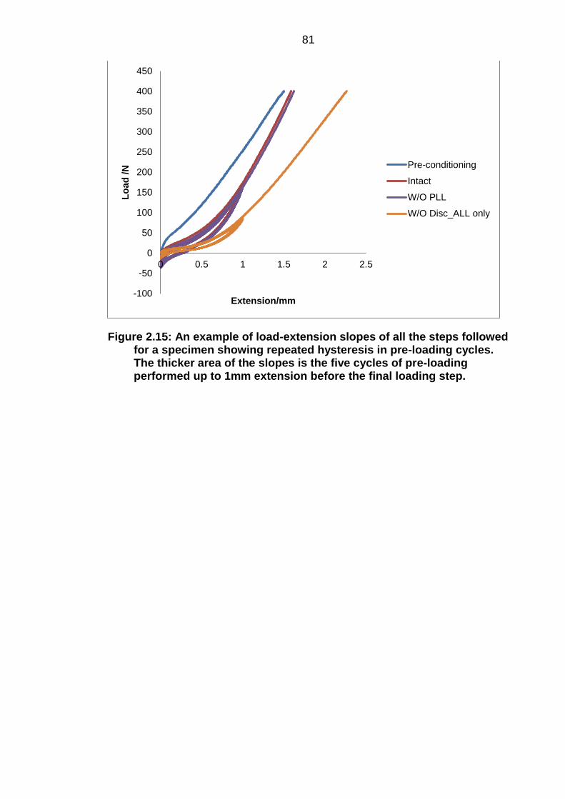
81
Figure 2.15: An example of load-extension slopes of all the steps followed for a specimen showing repeated hysteresis in pre-loading cycles. The thicker area of the slopes is the five cycles of pre-loading performed up to 1mm extension before the final loading step.
-100
-50
0
50
100
150
200
250
300
350
400
450
0 0.5 1 1.5 2 2.5
Lo
ad
/N
Extension/mm
Pre-conditioning
Intact
W/O PLL
W/O Disc_ALL only

82
Figure 2.16: The trimmed load-extension curves for all ALL specimens. The level and the spine the specimen was obtained from are indicated in the specimen name.
Table 2.2: The ‘toe region’ (k1) and final ‘linear region’ (k2) stiffness values, calculated by fitting least squares slopes to the post-processed load displacement curves of ALL, alongside the level and the spine the specimen was obtained from. The whole group mean and standard deviation (S.D.) are also shown.
Specimen Stiffness values for ALL (N/mm)
RMSE
R2
k1 k2
1: T2-3 30 82 1.64 0.998
1: T10-11 49 230 7.15 0.995
2: T3-4 73 179 5.19 0.998
2: T7-8 75 224 6.27 0.997
3: T1-2 20 66 1.99 0.997
3: T9-10 64 243 5.27 0.998
Mean ± S.D. 52 ± 23 171 ± 78
0
50
100
150
200
250
300
350
400
0 0.5 1 1.5 2 2.5 3
Lo
ad
(N
)
Extension (mm)
1: T2-3
1: T10-11
2: T3-4
2: T7-8
3: T1-2
3: T9-10

83
Figure 2.17: The trimmed load-extension curves for all PLL specimens. The level and the spine the specimen was obtained from are indicated in the specimen name.
Table 2.3: The ‘toe region’ (k1) and final ‘linear region’ (k2) stiffness values, calculated by fitting least squares slopes to the post-processed load displacement curves of PLL, alongside the level and the spine the specimen was obtained from. The whole group mean and standard deviation (S.D.) are also shown.
Specimen Stiffness values for PLL (N/mm)
RMSE
R2
k1 k2
1: T4-5 4 41 1.24 0.989
1: T8-9 43 85 0.78 0.999
1: T12-13 61 89 0.38 1.000
2: T1-2 12 40 1.89 0.993
2: T5-6 11 39 1.61 0.993
2: T9-10 30 67 0.82 0.998
Mean ± S.D. 27 ± 22 60 ± 23
0
10
20
30
40
50
60
70
80
90
100
0 0.5 1 1.5 2 2.5 3
Lo
ad
(N
)
Extension (mm)
1: T4-5
1: T8-9
1: T12-13
2: T1-2
2: T5-6
2: T9-10

84
Figure 2.18: Comparison of ovine and human (Pintar, et al., 1992) linear-region stiffness for both ALL and PLL showing mean stiffness values. Error bars depict standard deviation values.
2.7 Discussion
2.7.1 Discussion of testing methods and results
The published experimental studies (Chapter 1, Section 1.2.5) on mechanical
testing of ligaments provide a considerable amount of data on the
biomechanical parameters and mechanical properties of ligaments, however
the results are quite varied. Although the geometric parameters have been
calculated and presented, there is huge amount of variability across studies
due to difference in measurement procedures. Based on these results, it is
difficult to decide which method is the most accurate for testing. Although
dissection is never raised as an issue in any of these studies, based on the
observation and experience of this study, it is one of the most challenging parts
of mechanical testing of individual ligaments. The structure of the ligaments do
not follow the same pattern in the same specimen or across different
specimens. The fibres run in differing directions and interweave with fibres of
other tissues, such as discs, making the distinction between the two difficult.
They also tend to have different widths and thicknesses along the length
making it even harder to predict their boundary for accurate dissection of the
entire structure. The removal of ligaments from the spinal column for testing
often results in damage to the ligament.
Pre-tension in the ligament is another important consideration which is often
neglected in these studies. When the ligaments are removed for individual
ALL PLL
0
50
100
150
200
250
300
Sti
ffn
ess (
N/m
m)
Ovine
HumanLit.

85
testing, they lose the constant pre-tension they are under, in the intact state, in
spine which would make them retract and shorten (Tkaczuk, 1968). The ALL
and PLL have been shown to have a pre-strain of up to 10% and 13%
respectively (Tkaczuk, 1968). Therefore, keeping them in situ is essential to
obtain physiological behaviour, otherwise the stress-strain curves derived
would start at a different point to that if a pre-strain were applied first. Moreover,
the pre-strain is different for every specimen as it is shown to be dependent on
dimensions of the ligaments, the pressures within the nucleus pulposus and the
elasticity of annulus fibrosus (Tkaczuk, 1968), hence presenting data together
would not be comparable. Another disadvantage of individual ligament testing
is the difficulty of fixation, the ligaments either have to be removed with the
bony attachments or specialised clamping systems have to be employed to
avoid slippage of the specimen and damage of the specimen from the areas of
contact in the clamp. The technique is also unable to define the role of
ligaments in relation to other spinal components.
An in situ ligament testing method resolves most of the difficulties stated above
and was therefore the method of choice for this particular study. However, the
results obtained using this method showed quite a variability in initial load-
displacement behaviour at low strains. The load-displacement data recorded
was broadly compared to the published literature for ligaments to ensure the
loads obtained are reasonable and not due to a machine artefact. The initial
shape of the load-displacement curve appeared to be different to the shape
that is been published in literature, with a steep initial section prior to the toe
and linear region. This could have been due to the state of the disc, i.e. how
hydrated it was for a particular specimen, because both extension and load
were zeroed before starting the test. Different levels of disc hydration would
have affected the initial height of the specimen, and once the disc was sliced
through, there would be a change in the strain in the ligaments, so they are
potentially starting from different initial conditions hence the variation in results.
If the disc was compressed i.e. under-hydrated then it would push the vertebral
bodies to draw more water in but if it was overhydrated then it would pull on the
attaching structures. Although this initial high stiffness region does not tie in
with literature, it is difficult to make direct comparisons because authors have
not published their full load-displacement profile. Since this occurred at very
low strains, and was highly variable from one specimen to another, this region
was not considered in this analysis. Therefore, in order to make a comparison
across the specimens and with the published human data, the data was
consistently trimmed to remove the initial stiffer region and to define a ‘zero’
point that is consistent from one specimen to another.

86
The curves obtained after trimming the data all showed a characteristic shape
(Fig. 2.16 & Fig. 2.17), however, there was still quite a spread in the results
which is perhaps due to the natural variation in the specimens. Visually, the
ligaments tended to appear thicker and well defined towards the inferior of the
spine and the level is therefore also likely to affect the result. This is supported
by the stiffness results that generally showed a trend of increasing stiffness
with increasing level down the spine (see Table 2.2 and Table 2.3), although
this was not conclusive due to the small sample size. Most previous
researchers did not find a trend in spinal level and stiffness due to limited
sample size, however, Chazal et al. (1985) found each ligament at lower
thoracic or thoracolumbar level to be more resistant than the ligament of same
variety at any other level. Pintar et al. (1986) performed a histological study to
examine the composition of spinal ligaments in human. It was found that a
sample of LF from the upper cervical spine had very few elastin fibres
compared to the otherwise very high composition (50-60%) of elastin fibres in
the LF in other levels. This suggests that composition varies between spinal
levels, which might lead to different mechanical properties at different spinal
levels. Myklebust et al. (1984) studied spinal ligaments from 41 fresh human
cadavers and found the variation in strength and distensibility to be apparently
related to spinal geometry as they observed the strongest ligaments at atlanto-
occipital (C0-C1) and lumbar levels. Moreover, the size of the vertebrae (Gray,
1944) as well as the cross-sectional area of both ALL and PLL (Chazal, et al.,
1985) is found to be higher in the lumbar region of the spine. This indicates that
if size is considered to be the main factor affecting stiffness, then the stiffness
of the ligaments might be higher in the lumbar region. Also the natural variation
from one animal to another due to variances in weight, age and size is
unavoidable and might affect the stiffness outcome. Care was taken to choose
animals over 2 years old which would at least be fully mature for this study, but
further controls on variability were not possible.
The ALL appeared to be thicker than the PLL which was reflected in the mean
stiffness of ALL (171 ± 78 N/mm) being almost double to that of PLL (60 ± 23
N/mm).
2.7.2 Comparison to published human data
The main aim of this study was not only to characterise the ovine spinal
ligaments but also to compare the stiffness data obtained with published data
on human longitudinal ligaments. The stiffness data published in the literature
is mainly of the linear region of the force-displacement curve i.e. the k2
stiffness. The k2 stiffness obtained for both the ovine ALL (171 ± 78 N/mm) and

87
ovine PLL (60 ± 23 N/mm) of the thoracic region were both found to be stiffer
than published human ALL (33 ± 15.7 N/mm) and PLL (20.4 ± 11.9 N/mm) of
the lumbar spine (Pintar et al. 1992). In both these cases the ligaments were
tested in situ and in isolation and all supporting structures except the ligament
to be evaluated were sectioned. However, the loading rates in both cases were
very different with Pintar et al. (1992) using data that was tested at a faster rate
of 600mm/min as opposed to 1mm/min used for this study. An increase in
loading rate has been shown to increase the stiffness in cervical spinal
ligaments in similar isolated bone-ligament-bone samples (Butler, et al., 1988;
Mattucci, et al., 2012; Trajkovski, et al., 2014). If the same is true for the lumbar
spine, then the published stiffness by Pintar et al. (1992) would be lower if the
tests were to be carried out at a slower loading rate of 1mm/min. Also, as
described earlier, the stiffness appeared to change with the spinal level and if
the speculation above about stiffness of ligaments being higher in the lumbar
region holds true, then the stiffness for the human thoracic specimens would be
even lower than that stated above for human lumbar spine and hence certainly
lower than the ovine thoracic spine used in this study.
This potentially has repercussions if researchers are using the ovine spine as
an experimental animal model for spine research. For example, spinal
stabilization devices have been tested in ovine models to evaluate their
performance (Gunzburg, et al., 2009). If the ligaments are stiffer, then they are
likely to help with the stabilization, restricting the range of motion much better
than in the human spine. This means the spinal components which are
approved for clinical trial as a result of the success of testing in an ovine model
could fail in human as the stabilizing forces provided by human spinal
ligaments will be smaller. Therefore, the differences in the mechanical
properties between human and ovine ligaments should be borne in mind when
making a transition from the ovine model to the human.
2.7.3 Summary
In conclusion, a methodology for characterizing the mechanical properties of
spinal ligaments was developed and applied to ovine FSUs. Whilst there was
considerable variation in the results, the stiffness of both the ALL and PLL were
found to be higher than for human specimens, which may have implications for
the use of ovine FSUs for preclinical testing. The methodology developed in
this study will be used to test and extract the stiffness data for human spinal
ligaments (Chapter 4), enabling direct comparison between the ovine and
human data by removing the differences due to different testing regimes.

88
Chapter 3
Computational Methods Development and Results for Ovine
Longitudinal Ligaments
3.1 Introduction
This chapter presents the procedures that were used to devise a methodology
for developing specimen-specific computational models of the ovine spinal
ligaments using an image-based approach. The methods for micro-CT imaging
the specimens used in Chapter 2 are described, including an approach that
was developed to visualise the ligament clearly in the image data. The
methods for estimating the thickness of the ligaments over the disc region for
the purpose of segmentation as well as for the development of simplified-
geometry models are also presented. The image processing steps and
generation of the finite element models are then reported, with a particular
focus on the development of a methodology to best represent the experimental
setup in the computational model, to allow for a direct comparison of the model
predictions with the experimental outputs. An account of the sensitivity
analysis to understand the effect of varying geometric parameters, boundary
conditions, mesh size and material models is also given. The representation of
the ligament behaviour using various material models are described, starting
with a simple linear elastic model and building up to more complex material
models. The iterative approach used to determine the material model
parameters for each specimen are explained. The resulting material model
parameters are presented alongside the initial parameters derived by assuming
uniaxial behaviour.
3.2 Imaging Specimens
3.2.1 Introduction
Micro-computed tomography (µCT) is usually used in clinical or other research
studies for imaging bones. It provides high resolution volumetric information on
the internal microstructure of the sample by x-ray imaging taken at a series of
different projections. Computer algorithms are used to automatically reconstruct
the images as 2D image stacks or 3D volumes. The bone absorbs more x-ray
radiation than the soft tissues and the software by default assigns a brighter
colour to the pixels (or voxels in 3D) where the most energy is absorbed.
Hence, the bone appears brighter in the image while the soft tissue structures

89
such as discs, muscles and ligaments appear darker. As these soft tissues
have low X-ray attenuation in their native state, this makes their 3D imaging
challenging, especially when high resolution is required (Naveh, et al., 2014).
Contrast agents are often used to improve the visibility of soft tissue structures
and hence increase their contrast in µCT scans.
3.2.2 Imaging Protocol
Each specimen with PMMA plates on both sides was scanned using a µCT
system (SCANCO µCT100; Scanco Medical, Bassersdorf, Switzerland) to
provide images for the development of specimen-specific computational
models. The scanner settings used were as shown in Table 3.1. These settings
are the in-house standard for imaging spinal segments and have been shown
to consistently provide sufficient contrast between the bone and soft tissue for
image segmentation across a range of bone densities (Zapata-Cornelio, et al.,
2017). Using these settings meant there was the capacity to use greyscale-
derived bone properties in the FE models (Zapata-Cornelio, et al., 2017),
although it was not subsequently found necessary in this study. A good
contrast between different soft tissues is difficult to attain with the in-house CT
scanners and hence it was decided to use settings that were suitable for the
spinal bone and then use a separate protocol to visualise the ligament
structures of interest described in the following section.
Table 3.1: µCT scanner settings used on a SCANCO µCT100 device to
image FSUs with the ligaments intact.
The machine is calibrated monthly using a proprietary hydroxyapatite phantom.
The greyscales of the different concentrations of hydroxyapatite in the phantom
are compared to a calibration curve provided by the scanner manufacturer
(Scanco Medical, Bassersdorf, Switzerland). Any change in X-ray tube
performance will cause a drift the calibration and require the tube to be
replaced; this did not occur over the course of this study.
Energy (kVp) 70
Current (µA) 114
Integration time (ms) 300
Resolution (µm) 74

90
3.2.3 Use of Radiopaque Gel
3.2.3.1 Introduction
Initial scans were undertaken on the native tissue, however it was observed
that there was little contrast between the ligament and the background (air)
(Figure 3.1), therefore the use of a contrast agent was investigated to establish
if the contrast between ligament and background could be sufficiently improved
to allow clear visualisation of the ligament geometry.
The contrast agent used for this purpose was a radiopaque sodium iodide (NaI)
gel following successful preliminary trials of an in-house technique used to
visualise other soft tissues (personal communication with Dr Sami Tarsuslugil).
The gel used in previous projects was prepared with 0.2mol solution of NaI
(containing NaI powder and PBS solution) and low viscosity
carboxymethylcellulose sodium salt (CMC). The iodide ions have the ability to
be absorbed by the soft tissue and help improve their visibility on µCT because
of the improved x-ray attenuation. The improved visibility of the soft tissue gives
a better contrast with the background. The CMC component is used as a
gelling agent which give the solution sufficient viscosity to stay in place.
Figure 3.1: sagittal view taken from a µCT scan of an ovine vertebra, including the ALL and PLL, without contrast agent.
3.2.3.2 Method
In order to increase the contrast between the background and the ligament, a
study was designed to test the concentration of NaI gel such that the resulting
image had a greyscale halfway between the background and the bone. If it
were too dark, then the NaI greyscale distribution would overlap the
background greyscale distribution, making it difficult to segment the two using
image processing tools. Similarly if it were too bright, then the NaI greyscale
PLL ALL

91
distribution would overlap the bone greyscale distribution, again making it
difficult to segment the two using image processing tools. Mixtures with three
different concentrations of the NaI gel (0.2 mol, 0.4 mol and 0.6 mol solutions)
were prepared with an adequate amount of CMC so that the gel was sufficiently
thick to be able to stay in place when applied to a specimen. A few drops of
Indian ink were also added to the gel to make it distinguishable from the
specimen so it could be easily removed after application. The mixtures were
imaged individually alongside a small piece of vertebrae in the µCT scanner
and their contrast against the bone was observed (Figure 3.2).
The optimum concentration of NaI gel was then applied to a specimen to verify
that the gel provided sufficient contrast between the ligament and the
background. For this purpose, an FSU was fully cleaned, with as much as
possible of the muscle tissue removed carefully, leaving the ligaments intact.
The cleaned FSU was initially scanned under µCT without the contrast agent.
The ligaments were then painted with the NaI gel and left to rest for 20 minutes
so the iodide could be absorbed by the ligament tissue. The gel was then wiped
off so that there was no gel layer remaining on the surface of the ligament,
because such a layer would make it difficult to distinguish between the soft
tissue and the gel itself. The specimen was then rescanned.
3.2.3.3 Results
The results obtained for the study designed to test the concentration of NaI gel
are presented in Figure 3.2. The gel with 0.4 mol concentration solution was
found to give the optimum contrast.
Figure 3.2: Different concentrations of NaI gel in relation to the bone as seen on µCT scans with concentrations of (a) 0.2 mol, (b) 0.4 mol, (c) 0.6 mol.
After the application of the radiopaque gel with this optimum concentration to a
test specimen, it was found that the ligaments were distinguishable from both
the bone and the background. Figure 3.3 shows cross-sections through a
(a) (c)
Bone NaI gel

92
vertebral sample without (Figure 3.3(a)) and with NaI gel (Figure 3.3(b)) to
visualise the difference in ALL contrast post-application.
Figure 3.3: Cross-sections through a vertebral sample (a) without and (b) with NaI gel showing the difference in ALL appearance after the application of gel. In these images, the contrast has been increased and the bone has been segmented (red region) in order to provide a better contrast between the ligament and background for comparison.
3.2.3.4 Conclusion
The optimum concentration of 0.4mol was therefore used in subsequent
studies.
3.3 Determination of Ligament Thickness over Disc
3.3.1 Introduction
Although the application of contrast agent was useful in capturing the entirety of
the ligament, it was still difficult to draw a distinct boundary between ligament
and the disc from the µCT images. Thus it was not possible either to segment
the ligament over the disc region or to obtain a measure of the ligament
thickness that was required for the later development of a simplified-geometry
FE model. Two methods were explored in order to measure the thickness of
the ligament over the disc region.
3.3.2 Needle Indentation Test
The aim of this preliminary study was to measure the thickness of the ligament
over the disc as well as the bone regions to deduce if there was a difference in
thickness across the two regions.
ALL
(a) (b)
ALL

93
Method
In this method, a needle was used to pierce through the tissues and the applied
force measured to detect the change in response as the needle goes from one
medium to another, which in this case was from ligament to bone or from
ligament to disc (see Figure 3.4).
Figure 3.4: Needle-Indentation test (a) over the bone region and (b) over the disc region (b) to measure the thickness of (a) ALL and (b) PLL in both regions.
Results
The force-displacement response through ligament and through the bone was
found to have different gradients (Figure 3.5 (a)). Using this change in gradient
from one medium to another and from the initial point where the tip of the
needle touched the ligament, the thickness of the ligament could be derived.
However, this was not found to be the case with the ligament over the disc
region. Since the ligament and the disc have similar structure, a transition from
ligament to disc was not evident and a curve with an almost consistent gradient
throughout both tissues was obtained (Figure 3.5 (b)).
Conclusion
The thickness over the disc region could not be evaluated using the needle
indentation method and hence this method was discarded.
(a) (b)

94
Figure 3.5: Examples of force-displacement graphs of needle indentation into different tissues. (a) For the ligament-bone region: the transition from ligament to bone is apparent and could be used to calculate the thickness of ligament. (b) For the ligament-disc region: there is no transition of gradients, showing the similarity in the response from both ligament and disc.
Forc
e (
N)
Displacement (mm)
Transition from ligament to bone
(a)
Forc
e (
N)
(b)
Displacement (mm)

95
3.3.3 Photographic Image Analysis
The aim of this preliminary study was to measure the thickness of ligament
over the disc as well as the bone region using pixels in photographic images to
deduce if there is difference in thickness across the two regions.
Methods
An FSU specimen was sectioned in such a way that the disc was separated
from the vertebrae from one side i.e. by cutting through from the edge of the
disc. A photograph of the vertebra as well as the disc with the ligament
attached was captured with an aligned ruler using a SLR camera (Canon EOS
550D) with a high resolution lens (Canon 100 mm macro lens) (Figure 3.6 (a)).
A resolution of at least 14 pixels/mm was achieved. The ligaments on each
section were carefully tinted with a fine-nibbed black marker pen, prior to
capturing the image, so it could be easily differentiated from the attaching disc
or bone. An image analysis tool (ImageJ 1.41, Wayne Rasband, National
Institutes of Health, USA) was used to measure the thickness from the pixels in
the pictures. The images were imported to the software and the pixels in the
image were calibrated using the reference scale in the photograph. The
thickness was measured in pixels sagittally over six different regions of the disc
section as well as over the corresponding bone section. The pixels were
converted into respective values in millimetres and mean values were
calculated and compared across both the disc and the bone region. An
example of the process is illustrated in Figure 3.6.

96
Figure 3.6: Process of measuring the ligament thickness: (a) sagittal view of the disc section (left) and PMMA-cemented-bone section (right), (b) calibration of the image from pixels to mm, (c) measurement of the ligament thickness over the disc region, (d) measurement of the ligament thickness over the bone region.
Results
The results for the photographic analysis of the ligament thickness are
presented in Table 3.2. The mean thickness value of the ligament over the disc
(1.05 ± 0.05 mm) was found to be very similar to the mean thickness of the
ligament over the bone (1.04 ± 0.07 mm).
Table 3.2: Thickness values of a ligament obtained after conversion from pixels to millimetres over disc and corresponding bone regions.
Measurement Region
I II III IV V VI Mean
Thickness Over Bone (mm)
1.13 1.04 1.01 1.11 1.01 1.02 1.05±0.05
Thickness Over Disc
(mm)
1.09 0.99 1.06 1.14 1.02 0.95 1.04±0.07
Conclusion
The results indicated that there was little difference in the thickness along the
length of the ligament and therefore the measureable thickness in the vertebral
region could be used for the disc region where the thickness could not be
measured directly from the CT images.
1.13mm 1.06mm
83.336 Pixels = 5mm

97
3.3.4 Discussion
Two studies were carried out to deduce the thickness of the ligament over the
disc region from the vertebra-bone region. The needle indentation test failed to
output the thickness over the disc region due to similar fibrous composition of
disc and ligament, hence this method could not be adopted. The photographic
image analysis method showed very little difference in the thickness of the
ligament across the two regions. This method was likely prone to some human
error and the accuracy with which the edge of the marker pen line could be
lined up with the observed ligament boundary. Experiments were undertaken to
quantify this error by using the same marker pen to follow a given line on a
piece of paper. It was found that the deviation from the line was less than
0.06 mm, indicating the likely accuracy of this technique. To further develop
confidence in this method of image analysis, the thickness of the ligament from
the FSU used in this study was also measured from a sagittal cross-section of
its microCT image close to the disc using an image processing package (Scan
IP version 7.0, Simpleware, UK). The average thickness over the disc section,
measured from ScanIP, was compared with the thickness obtained from the
photographic image analysis method (Table 3.2) and it was found to be less
than 0.032 mm. This provided further confidence in the photographic method
and in the conclusion that there was little change in ligament thickness between
bone and disc regions.
3.4 Image Segmentation
3.4.1 Images Pre-processing
The reconstructed µCT images of the specimens were subjected to some
preliminary preparations before being segmented. This included conversion of
the images from the µCT scanner format (*.DICOM) at the same resolution
(74µm) to an alternative format (*.TIFF) using a code developed in-house
(Matlab 7.9, MathWorks, USA; Jones and Wilcox 2007). This reduced the
number of greyscale values present in the images from 64,000 (Hounsfield
units) to 256, i.e. reducing the number of grey shade variations in the greyscale
spectrum.
The image data in *.TIFF format was then exported to an image processing
package (Scan IP version 7.0, Simpleware, UK) (Figure 3.7 (a)). The software
enabled the images to be segmented and the vertebra and the morphology of
the ligaments to be identified. The image data was first cropped to remove both
the side plates leaving the image area only covering the ligament to be

98
segmented i.e. either the ALL or PLL and small sections of attaching superior
and inferior bones and disc (Figure 3.7 (b)).
Figure 3.7: (a) µCT sagittal view of an FSU with the PMMA cement on each end, (b) cropped image of (a) following removal of the cement and unwanted regions leaving the image area only covering the ligament to be segmented and small sections of attaching bones and disc.
The following segmentation procedure was adopted to create segmented
images (referred to here as ‘masks’) of the vertebral bone and ligament of
interest.
3.4.2 Segmentation of the Bone
An iterative method was used to find the optimum upper and lower threshold
values to capture the bone by visual comparison between the mask and the
underlying image. These values were then used with an active thresholding tool
(‘paint with threshold’) on all the image slices to create a mask capturing the
bones of both the superior and inferior vertebra (Figure 3.8 (a)). A floodfill tool
was then used to remove unwanted islands and to separate the superior and
inferior vertebra into separate masks (Figure 3.8 (b)). Further segmentation
methods including morphological close, cavity fill and floodfill, were performed
as required to obtain fully closed bone masks with no holes and or gaps.
Figure 3.8: Segmentation of bone (a) after the use of thresholding to
capture the bone tissue only, and (b) after the use of floodfill, to separate
inferior and superior vertebra masks, and after closing all the respective
holes and gaps.
(a) (b)
(a) (b)

99
3.4.3 Segmentation of the Ligament
The segmentation of the ligament using automated tools was found not to be
possible because the greyscale distribution of the ligaments overlapped those
of the disc, the trabecular bone spaces and also some background noise.
Therefore, a semi-manual approach was required to segment the ligament.
One potential option was to use the ‘paint with threshold’ tool manually on all
individual slices. However, this was found to be an immensely time-consuming
and labour-intensive process as each specimen contained over 250 slices in
the vertical direction. After some iterations, the procedure below was found to
be the optimum for segmenting the ligaments efficiently with the fewest manual
procedures:
The threshold operation was first applied iteratively over the whole
image to determine the most appropriate values for capturing the
ligament of interest i.e. either the ALL or PLL.
The ‘active thresholding tool’ was then used with these values on
individual image slices to create a mask over the ligament region on that
slice. The procedure was repeated on every 5th slice over the bones
area only (Figure 3.9). To save more time, the approach was also tried
on every 20th slice and then on every 10th slice, but the post-processing
steps that followed were found to be more time-consuming and labour
intensive compared to the ones that followed painting on every 5th slice.
A morphological close operation of 5 voxels in the direction of the slices
was then performed on the ligament to join the painted segments
resulting in a mask over both superior and inferior bone area.
Figure 3.9: ligament mask manually painted over every 5th slice of bone region only.
A further morphological close operation in the direction of the slices was
then performed between the lower ligament slice of the superior
vertebrae and the uppermost ligament slice of the inferior vertebrae to
join the painted segments. This resulted in a mask representing the
ligament over the disk region.

100
Further segmentation was performed including the use of morphological
close, cavity fill and floodfill functions, to obtain fully closed ligament
masks with no holes or gaps.
A ‘subtract’ Boolean operation was performed on the ligament and each
vertebra in turn in order to remove any overlapping regions (yellow
regions in Figure 3.10 (a)) between the ligament and the bones (Figure
3.10 (b)).
An ellipsoid was created between the two bones to represent the disc,
keeping the ellipsoid parameters within the boundaries of the bones as
shown in Figure 3.11 (a) because the thickness of the ligament was
shown to be very similar over the bone and the disc region (Section 3.3).
Any overlapping region between this ellipsoid-disc mask and the
ligament mask (blue region in Figure 3.11 (b)) was removed using
Boolean operations, to cut away any remaining ligament mask from the
disc region, thus preserving the disc mask while reducing the ligament
mask (Figure 3.11 (c)). This creation of an ellipsoid mask was only
required in the case of the ALL because the anterior aspect of disc is
curved in reality, therefore it was important to reflect this shape in the
ligament mask. Whereas, in the case of the PLL, the creation of an
ellipsoid was not required because the posterior aspect of the vertebra
and the disc region are flat. Here, it was found that a morphological
close operation resulted in an accurate representation of the PLL shape.
Figure 3.10: segmentation of ligament (a) before and (b) after the application of ’Boolean operations’ whereby the yellow regions show the overlapping regions between the bones and the ligament.
(b)

101
Figure 3.11: (a) creation of an oval shape between the superior and inferior vertebrae to represent disc, (b) the overlapping region (blue area) between the disc and the ligament, (c) final ligament mask after using ‘Boolean operations’ to remove the unwanted region.
3.5 Image Downsampling
The segmented images were then down-sampled to an optimum resolution at
which image pixel-size could be reduced without losing the detail of the
ligament. The downsampling operation was performed to help govern the size
of the finite element mesh and to speed up subsequent processes in ScanIP.
The optimum was established by down-sampling the image from its original
resolution of 0.074 mm to a set of resolutions between 0.1 and 1 mm, in
increments of 0.1 mm, and comparing the mask on the ligament visually. A
resolution of 0.6 mm was found to be the optimum because it was the lowest
resolution to which the image could be down-sampled before there were visual
discontinuities in the overall shape of the ligament. An example of this is shown
in Table 3.3.
A number of different downsampling methods were also investigated using
built-in algorithms within the software. The ‘majority wins’ interpolation was
found to be the most optimum (see Table 3.4) because it had the least effect on
the overall volume of the ligament, which was of greater importance in this
study than the bone or disc in the overall behaviour of the model. However, the
down-sampling procedure still resulted in severe discontinuities in the voxels,
especially in the ligament (Figure 3.12). The down-sampled images were
dilated and smoothed using built-in features to remove the discontinuities,
hence pre-smoothing the image prior to the creation of a mesh. The final 3-D
segmented models of the ALL and PLL are illustrated in Figure 3.13 (a) and (b)
respectively, at the point prior to meshing. Visual comparison back to the
underlying image showed that after these procedures, the mask was a good fit
to the ligament boundaries.
(a) (c) (b)
Overlapping region

102
Table 3.3: An example of image downsampling from original resolution of 0.074mm to how the optimum of 0.6mm was arrived at.
Original Image 0.2mm Resolution 0.4mm Resolution
0.6mm Resolution 0.7mm Resolution 0.8mm Resolution
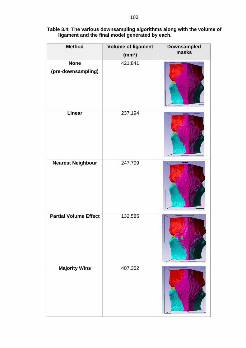
103
Table 3.4: The various downsampling algorithms along with the volume of ligament and the final model generated by each.
Method Volume of ligament
(mm³)
Downsampled masks
None
(pre-downsampling)
421.841
Linear 237.194
Nearest Neighbour 247.799
Partial Volume Effect 132.585
Majority Wins 407.352

104
Figure 3.12: Discontinuities in the ligament mask as a result of downsampling.
Figure 3.13: Final 3-D volume of the masks after dilate and smoothing tools have been applied, showing (a) the ALL, superior vertebra, inferior vertebra and disc, (b) the PLL with superior and inferior vertebrae.
(a) (b)

105
3.6 Finite Element Method Development
The methodology for developing an FE model of the longitudinal ligaments was
initially developed from the images of a FSU where the ALL was tested
(Chapter 2). Sensitivity analyses were initially carried out on simple linear
elastic material models of the ALL with both idealised rectangular geometry and
a more realistic representation of the geometry, to test how the geometry,
boundary conditions and applied load could be best simplified to represent the
experimental setup accurately. The finite element mesh size was also
examined. In addition, a series of non-linear material models (as described in
Chapter 1, Section 1.2.7) were applied to the model to decide which material
models were suitable. Combining the best choice of boundary conditions,
loading and material model, a methodology was hence devised for generating
specimen-specific models of the ligaments that could then be used to
determine the material properties as described in Section 3.7.
The devised methodology was then also applied to a model of the PLL
exported from ScanIP to demonstrate that the methodology could be replicated
and would be appropriate for other ligamentous tissues.
3.6.1 Sensitivity Analysis
Four different sensitivity studies were carried out to develop a methodology that
best represented the experimental setup in order to derive the material
properties of the ligaments.
i. Study I – sensitivity to dimensions
ii. Study II – sensitivity to boundary conditions
iii. Study III – mesh sensitivity
iv. Study IV – choice of material models
3.6.1.1 Study I - Sensitivity to Dimensions
The aim of this study was to determine how the geometry, i.e. the dimensions
and shape of the ligament, affect the overall behaviour of the ligament. Two
rectangular models, with idealised ligament geometry, and a third model based
on the specimen image data were developed. All three models had the same
total length and same average cross-sectional area. The rectangular models
were compared to simplified theoretical calculations based on one-dimensional
assumptions to understand if the change in physical dimensions affected the
output of the model. The results obtained from all three models were also
compared against each other to quantify the difference in predicted stiffness, if
any, that was caused by the geometric simplifications.

106
Model Geometry:
For the two idealised rectangular models (Rec_A and Rec_B), parameters
were derived from a lateral view of the masked image of the ligament in ScanIP
(Figure 3.14 and Table 3.5); these included the length (Ln), maximum and
minimum thickness (tmax and tmin respectively). From the mask volume and
length, an average area was also determined.
Figure 3.14: Sagittal view through segmented microCT image showing the measurements used for the development of the equivalent rectangular models (Ln = length, tmax = maximum thickness, tmin = minimum thickness).
Table 3.5: Geometric parameters used for the development of idealised rectangular models of ligament.
Volume (V, mm3)
Length (Ln, mm)
Maximum Thickness (tmax, mm)
Minimum Thickness (tmin, mm)
Average Area (A, mm2)
124.1 23.49 1.31 0.17 5.22
The two models were built to represent the two extremes of the ALL thickness.
The length used for both models was the same, with the thicknesses as given
in Table 3.5 and the widths were calculated as follows:
For thickest model, Rec_A; WA = 3.97 mm
For thinnest model, Rec_B; WB = 31.46 mm
The realistic geometry model, Real_A, was obtained as a result of
segmentation and downsampling in ScanIP (Section 3.4 and Section 3.5).
Mesh:
The models, Rec_A and Rec_B, were both meshed using hexahedral elements
while Real_A was meshed in ScanIP employing the ScanIP meshing tool with
tmax
Ln
tmin

107
in-built meshing algorithm, +FE Grid, which converted the segmented masked
regions of the FSU directly into an FE volumetric mesh. This resulted in
meshes comprising 4-node tetrahedral and 8-node hexahedral linear elements.
Figure 3.15 shows the full meshed model. Surfaces were also defined at the
two extremes of the model i.e. the top and the bottom surface to be used for
the application of load and possible boundary conditions. The models were
exported from the ScanIP as FE input files for Abaqus. The meshed vertebrae
were then deleted in Abaqus to leave only the model of the ligament, still
containing the definitions of the surfaces, that was used in this study.
Figure 3.15: Final meshed model of ALL ready to be exported.
Material Properties:
Although the ligament behaves in a non-linear elastic manner, an isotropic
linear elastic material model was used for this initial study to simplify the
material behaviour before a more realistic representation of material behaviour
was devised. To describe a linear-elastic model in Abaqus, two independent
material parameters, the Young’s modulus (E) and Poisson’s ratio (), were
required. The Young’s modulus was taken as typical value of 0.4 GPa from
Chapter 2 and the Poisson’s ratio was assumed at 0.3 based on literature
(Tusang et al., 2009).
Boundary Conditions and Applied Load:
Figure 3.16 shows the boundary conditions (BCs) and load applied to the
models. The bottom surface was fully encastre, i.e. constrained in all degrees
of freedom, to stop any movement in order to represent the fixed inferior
vertebra in the materials testing machine (Chapter 2, Section 2.3.4, and Figure
2.4). The top was fixed such that it was allowed to move in the upward direction
only i.e. in the direction of the applied load to represent the movement of the

108
superior vertebra in upward direction only due to the application of the tensile
load in the experiment.
All three models, Rec_A and Rec_B and Real_A, were subjected to an upward
concentrated force of 400 N. The force was applied to the top surface of
ligament through a rigid plate created in tied contact and placed centrally over
the top surface of the ligament. This was a simplified representation of the
tensile load applied in the experimental setup as described in Chapter 2
(Section 2.3.4). The application of load via a plate tied directly to the surface
was found to be easier as it distributes the load applied over the entire surface
that it is tied to, compared to applying the loads to each individual node over
the surface.
Figure 3.16: Boundary conditions and loads applied to models (a) Rec_A, (b) Rec_B and, (c) Real_A.
Theoretical Analysis of Rectangular Models:
Both the rectangular models were developed using the same cross-sectional
area and length, with the same modelling parameters, therefore, if the models
were under perfect uniaxial stress, then both should extend by the same
amount. The displacement was calculated using Equation 3.1, assuming
uniaxial stretch, and compared to the displacement from the models in the
direction of the stretch (U3) given in Table 3.6;
σ = F/A = 0.4/5.22 = 0.766 kN/mm2
E = σ/ε
=> ∆L = (σ x L)/E = 4.45 mm [eq. 3.1]
Where,
σ = stress
F = total force applied to the ligament
A = cross-sectional area of the ligament
E = Young’s modulus
(a) (b) (c)

109
ϵ = strain
L, ΔL = original length, change in length
Results:
The results obtained in the form of contour plots for all three models (Rec_A,
Rec_B and Real_A) are presented in Table 3.6. The results are only presented
for the direction in which the force was applied, z-displacement (U3). The x
(width) and y (thickness) displacements are difficult to interpret due to shape
and orientation of ligament.
The theoretical displacement in the direction of the force applied was found to
be 4.45 mm. The displacement for both Rec_A (4.42 mm) and Rec_B
(4.30 mm) were very similar to the theoretical value, however, Rec_A gave
results closer to the theoretical results assuming uniaxial stretch.
The realistic geometry model, Real_A, resulted in a U3 displacement of
14.5 mm which was over three times higher than both the theoretical
calculations and the rectangular model outputs.
Table 3.6: Contour plots obtained for Rec_A, Rec_B and Real_A alongside the scale in mm showing displacement in the direction of stretch (U3)
Discussion:
The study indicated that the behaviour of ligaments in the modelled regime, i.e.
in extension, is sensitive to the geometry used. There are two possible
irregularities in the real ligament due to its:
1. irregular cross-sectional area and
2. curved shape (curved in several different directions).
Although it is difficult to separate these two factors from the results, an
approximation of the curvature along the length of the ligament could be made
to evaluate its effects. When the real ligament is stretched without any contact
Model Rec_A Rec_B Real_A
Displacement in the direction of stretch (U3/mm)

110
with the bone, it will straighten out. Assuming it to be an arc (Figure 3.17) then
its length (a) (i.e. the length of the ligament prior to stretching), can be worked
using the expressions given in Figure 3.17. The dimensions of ligament from
the realistic model used in this study were measured as shown in Figure 3.18.
This gives a chord length (c) of about 23 mm (See Table 3.5) and curve height
(h) of ~1.6 mm, resulting in the initial length of the ligament (a) being ~23.3
mm. This means that theoretically a displacement of 0.3 mm could be applied
purely to straighten it out, prior to causing any axial strain within the material.
However, this displacement is small compared to the amount the ligament
actually stretched by (14mm - see Table 3.6, U3 for Real_A); therefore, it can
be seen that the curvature alone cannot explain the disparity with the
rectangular models, and the irregular cross-section must also play an important
part.
Figure 3.17: Expressions to theoretically calculate the approximate length of ligament (a) post-stretching, assuming it to be part of a circle.
Figure 3.18: Lateral view of a meshed ligament in Abaqus to measure the curved distance between top and bottom of ligament i.e. length of ligament (c) and difference between the ends and middle of the ligament (perpendicular distance between lines) i.e. curve (h) of ligament. The green region shows the meshed anterior side of the ligament.
Conclusion:
h
c
a
r r b
Formula for segment radius (r) by chord and height:
r =h
2+
c2
8h
Segment angle:
b = 2 arcsinc
2r
Arc length:
a = br
h
c

111
The irregular shape of the ligament i.e. the varying cross-section as well as the
irregular curved shape of ligament, is an important consideration while
modelling its overall behaviour hence a simplified geometry could not be used
to derive the material properties of the ligament.
3.6.1.2 Study II – Sensitivity to Boundary Conditions
The aim of this study was to test the sensitivity of the ligament behaviour to the
boundary conditions (BCs) applied. Two models with different lengths but same
width and thickness were developed and differing boundary conditions were
applied. The work was carried out on rectangular models for the ease of
modelling and subsequent meshing. The results in the form of displacement in
the direction of stretch were compared between both models in order to
quantify the differences, if any, made by varying the way the boundary
conditions were applied and also to see if the realistic ligament model could be
simplified by reducing it to just the region corresponding to the disc. This
formed the basis of subsequent modelling on the realistic geometry.
Model Geometry:
Two rectangular models were developed, a long rectangular model with the
same dimensions as Rec_A (Rec_C) and a short rectangular model which had
the same length as the section of ligament between the vertebrae (Rec_D).
Long-Rectangular model (Rec_C)
In reality, the longitudinal ligaments are attached to the superior and inferior
vertebrae and disc on one side while they are free on the other. In the
experiments reported in Chapter 2, the force was applied to the ligament via
the stiffer superior-vertebra bone while the inferior-vertebra, attached to the
bottom section of the ligament, was held in place, leaving the central region
(corresponding to the attachment to the disc) free, so this is the main region of
stretch. A schematic representation of this is shown in Figure 3.19 (a). To
represent these conditions in model Rec_C, a discrete rigid plate was
generated and placed centrally, in tied contact with the upper region of the
model corresponding to the attachment region of the superior vertebra (Figure
3.19 (b)). The dimensions of the plate were kept slightly bigger than this
surface of the ligament to ensure the full surface was attached.
Short-Rectangular model (Rec_D)
The length of the region corresponding to the attachment of the disc was
measured from ScanIP and a rectangular model, Rec_D, with the same
thickness and width as model Rec_A but new height (corresponding to the disc
length) was generated.

112
Material Properties:
The same isotropic linear elastic material model, as previously used in study I,
was used for both models in order to make the results comparable between the
models.
Boundary Conditions and Load Applied:
Rec_C
An encastre constraint was set on the surface of the lower section which
represented the area covered by the inferior vertebra to replicate the
attachment with the inferior vertebra. The middle section which represents the
area covered by disc was left free as in the experiment. The load was applied
centrally on the plate in the upward direction to represent the load applied to
the ligament, in reality, via the superior vertebra. The plate was restricted to
move in the upward direction only. The model is represented in Figure 3.19 (c).
Figure 3.19: Schematic of the Rec_C model boundary conditions. (a) Ligament with bone and disc attachment regions identified, (b) image of model with side-plate tied to the top region, (c) front view of model with BCs and load.
Rec_D
The same BCs and load were applied to model Rec_D as applied to the initial
simplified rectangular model, Rec_A. That is, encastre boundary conditions
were applied to the bottom end of the model Rec_D to stop any movement,
while the top was allowed to move only in the direction of the applied load. The
load was applied to the top surface of the model through a rigid plate created in
Region for the
attachment of
superior-vertebra
Region for the
attachment of
inferior-vertebra
Region for the
attachment of
disc
(a)

113
tied contact and placed centrally over the top surface. The same load of 400N,
as previously used for Study I, was applied to both the models.
Mesh:
For Rec_C, the model was meshed using same number of hexahedral
elements as for Rec_A. For Rec_D, the model was meshed using same
number of hexahedral elements as were present in the disc region of the model
Rec_A.
Results:
The results obtained are presented in Table 3.7. The results for model Rec_C
showed that the section of the ligament left free i.e. the region that corresponds
to the attachment of the disc experienced higher strains, as expected.
Analysis:
Comparing the results of Rec_D with Rec_C (Table 3.7) showed that the
overall behaviour was similar with similar contours observed in the free
(stretched) section of ligament in both cases. However, the displacements were
found to be very different in the two cases. The displacement U3 obtained for
Rec_C (0.756 mm) was found to be higher than the displacement obtained for
Rec_D (0.321 mm). Moreover, Rec_D shows close to constant U3
displacement across the thickness while Rec_C exhibits big differences in
displacement between its anterior and posterior sides. This is due to the way
the load was acting on the two models; in Rec_C, it was effectively pulling just
one edge of the middle section of the ligament, whereas in Rec_D, the force
was applied across the full width.
Conclusion:
The study showed that changing the boundary conditions from simplified to
more realistic ones varied the loading applied in all directions which ultimately
affected the overall stretch of the ligament in the principal direction. This
indicated that the application of realistic boundary conditions is required to
represent the true behaviour of the ligaments in order to derive the material
properties of ligament accurately.
This study also showed that the use of only the middle section is not suitable
for modelling the behaviour of the full ligament, therefore the realistic-geometry
model of the ligament would have to capture the entire height of the ligament.

114
Table 3.7: The displacements in the x (U1), y (U2) and z (U3) directions obtained for Rec_C and Rec_D showing that the greatest variation occurs over the section corresponding to the disc region.
Displacement-
Rec_C (mm)
Displacement-
Rec_D
(mm)

115
3.6.1.3 Study III – Mesh Sensitivity
The aim of this study was to analyse the sensitivity of the material to the type
and size of mesh used and obtain a minimum mesh size that could be used for
all the FE models.
Model Geometry, Boundary Conditions, Loads and Material Properties:
The study was carried out on a simpler model that was found to represent the
experimental behaviour closely i.e. model Rec_C with the same boundary
conditions and loads as previously used in Section 3.6.1.2. The same isotropic
linear elastic material model, as previously used in Study I was used. The
realistic geometry was not used because it is difficult to control the mesh size in
ScanIP where there is a complex shape involved, as one can only limit the
maximum element size. Since each model will have different geometry, the aim
of mesh convergence was to look at a generic case that could then be applied
as a maximum size across all models. Moreover, in re-meshing the model in
ScanIP, the capture of the geometry also changes (with finer features being
captured at higher resolutions), and this is also affected by the underlying
image voxel size (Jones & Wilcox, 2007), so there are two factors changing:
the geometrical representation and the number of nodes (degrees of freedom).
The Rec_C model has a regular geometry, it is not based on image data and
the shape does not change with increasing mesh size, so the effects of the
number of degrees of freedom can be isolated; it was therefore deemed most
suitable for this study.
Element Type:
Tetrahedral elements are best for modelling complex geometry due to their
ability to conform to irregular shapes with little distortion. However, the space
generated by tetrahedral elements typically requires 4–10 times more elements
than a hexahedral mesh to obtain the same level of accuracy (Cifuentes &
Kalbag, 1992; Weingarten, 1994), implying that hexahedral elements are more
efficient. Different orders of both types of elements are available with the higher
order elements requiring more sophisticated shape functions, however, higher
order means more integration points and hence an increasing computational
cost (ABAQUS, 2014). The in-built meshing tool in ScanIP uses a mixture of 4-
node tetrahedral and 8-node hexahedral linear elements to achieve a
compromise in accuracy and computational cost. Both these element types
were explored to find the optimum mesh size that would be used in further
modelling.

116
Mesh Size:
Both hexahedral and tetrahedral elements were generated on the Rec_C
model with increasing number of elements (mesh size). The output of interest
was the displacement in the direction of stretch (U3) since this was the only
parameter used and compared to experimental data in the subsequent analysis
within this thesis. For both types of elements, the mesh size was increased until
solution convergence for the output of interest was achieved.
Results and Analysis:
The results obtained for both element types were plotted on the same graph
(Figure 3.20). It can be seen that the hexahedral and tetrahedral element types
converge to very similar displacement (respectively ~0.703 mm and ~0.698 mm
- less than 1% difference). Since tetrahedral elements are stiffer (Carl, et al.,
2006), for a given applied load, one would expect a smaller displacement for
the tetrahedral mesh as was seen in this case. Hexahedral elements as
expected, converged at a lower element count of under 20,000 elements, as
compared to the tetrahedral mesh where a steady increase in displacement
was achieved until around 750,000 elements and there was still an increasing
trend even at 850,000 elements. To translate the findings from this simple
study to the FE analysis of realistic-geometry models, a maximum element size
was required since this could be controlled in ScanIP, an error of less than 5%
in the output was deemed acceptable, because other factors in the experiment
would likely produce considerably higher errors than this, such as the
simplification of the boundary conditions, hence having a highly converged
mesh would not have a significant effect on the accuracy of the FE analysis.
Using the output of the converged hexahedral mesh as the target, any models
achieving a displacement above 0.668 mm would therefore be deemed
adequate. For the tetrahedral mesh, this was achieved with greater than ~5000
elements for the Rec_C model, equating to an element size of 0.5 mm or
smaller.

117
Figure 3.20: Mesh convergence study on simple rectangular model, showing the predicted U3 displacement (note: U3 scale does not start at zero) for models using hexahedral and tetrahedral elements.
Conclusion:
From this study, it was found that an element size of less than 0.5 mm would
provide adequate convergence of the axial displacement for both tetrahedral
and hexahedral elements. It is important to note here that the focus of this
study has been only on displacement so if future studies have interest in other
output fields e.g. stress or strain, then further convergence tests would be
necessary.
3.6.1.4 Study IV - Choice of Material Model
The aim of this study was to test various material models available in the
Abaqus software and identify the ones that best represent the experimental
behaviour of the ligament.
Model Geometry:
The study was carried out on the idealised rectangular representation of
ligament due to the ease of model development and implementation. The
model Rec_C represented a reasonable representation of the BCs and load
applied to the experimental system, however, this setup could not be replicated
in the realistic-geometry FE model due to the irregular shape of the ligament
6.40E-01
6.50E-01
6.60E-01
6.70E-01
6.80E-01
6.90E-01
7.00E-01
7.10E-01
0 200000 400000 600000 800000 1000000
U3 (
mm
)
Element count
Hexahedral Elements
Tetrahedral Elements

118
which meant it could not be tied with a straight side-plate. Therefore, the model
was adapted to more closely represent how a real irregular shaped ligament
could be modelled. This model, Rec_E had the same geometry as Rec_A and
Rec_C, but with the addition of a rectangular part, attached to the top region, to
replicate the superior-vertebra. A schematic of the model is given in Figure 3.21
(a).
Boundary Conditions and Load Applied:
A load of 400N, as in previous tests, was applied to the rectangular part
representing the vertebral bone via a rigid plate tied to the top surface of the
idealised rectangular vertebra. This replicated the load applied to the ligament
via the superior-vertebra. The BCs defined on other regions were the same as
in the case of Rec_C. The top plate in this case was restricted to move only in
the direction of stretch. The model with boundary conditions and loads is
represented in Figure 3.21 (b).
Material Model:
The idealised vertebra was made near-rigid by assigning it a linear elastic
Young’s modulus of 400 GPa i.e. 1000 times that of the ligament. This was to
make sure that this structure represented the stiffer bone during the stretching
of the ligament. A Poisson’s ratio of 0.3 was applied to the bone.
The ligament was assigned different material models as described below:
The linear elastic material model used in previous studies was applied to
the ligament geometry in order to make a comparison with previous
simplified models.
The ‘non-linear geometry’ option in the finite element solver was turned
on and the model was re-run to see the effects, if any, that this option
had on the outputs. This option is an additional requirement for running
hyperelastic or hyperfoam models and is optional for linear elastic
models.
A hyperelastic neo-Hookean model was evaluated because this model
has been used previously in finite element modelling of knee ligaments
(Chapter 1, Section 1.2.7).
Two further hyperelastic models (Mooney-Rivlin and Ogden) were
evaluated because they have also been shown to be effectively used in
the modelling of ligaments (Chapter 1, Section 1.2.7).

119
A hyperfoam material model which was shown to have a similar
structure and response to the ligament (Chapter 1, Section 1.2.7) was
also tested.
Figure 3.21: (a) Schematic of ligament with idealised rectangular bone to represent superior-vertebra. (b) Rec_E model with load applied to the reference point on top via a rigid plate and encastre BCs on the inferior vertebra and the restriction of the reference point at the top to move in the directions of the stretch only.
Within the Abaqus software, the coefficients for both the hyperelastic and
hyperfoam models could be determined directly from the input of the test-data
in the form of nominal stress and nominal strain. The test data was obtained by
using a typical load-extension data set from the experimental results, and the
cross-sectional area and length used previously for the construction of the
rectangular ligament models such as Rec_A, assuming the ligament to behave
as a uniform and uniaxial structure. This load-extension data was obtained from
the same specimen as was used to generate the realistic-geometry model as
well as the dimensions for the simple models. A Poisson’s ratio of 0.3 was used
to define the compressibility in each case.
Using the in-built algorithm within Abaqus, the material parameters for the
hyperelastic and hyperfoam models were derived from the input test-data. A
curve-fitting algorithm was used to gain the best fit to the inputs. The software
outputted the predicted curve for each model alongside the input (test-data)
Region corresponding to inferior-vertebra
Idealised rectangular part to represent superior-vertebra
(a)

120
curve (Figure 3.22). The best-fit curve for each material model and the input
experimental curve were then compared to see how accurately the material
model could describe the curve based on the coefficients derived by the
Abaqus software. The hyperfoam material model behaviour could not be
predicted automatically from the input without simulation, because this option is
not currently available in Abaqus. Therefore, this material model was directly
applied to the FE model and the material parameters used by Abaqus were
obtained from the .dat file of the FE model.
Implementation of Material Models:
The material models which were found to closely follow the behaviour of the
ligaments (see Figure 3.22) were then applied to the Rec_E model and the
results obtained, in the form of force-displacement behaviour, were compared
against the experimental data. To extract this data, the time-displacement
values over the reference-node where the load was applied were obtained. The
time-displacement curve was converted into a force-displacement curve by
multiplying the proportion of the time step by the applied load. The same
procedure was repeated for the simulation of FE models with the hyperfoam
material behaviour. This provided a means by which to examine if the material
parameters could be derived by assuming the experimental data was a uni-
axial test on a uniform geometry test-piece, or if the structure and geometry of
the ligament meant the uniaxial assumption would be incorrect.
Results:
The linear elastic material model was unable to solve when the non-linear
geometry option was not selected. The use of non-linear geometry option with
the linear elastic model gave similar contours as were observed in the case of
the Rec_C model however, the local strains over the disc region as well as the
displacements were higher in this case due to more realistic attachment to the
upper vertebra being used.
When the hyperelastic Neo-Hookean model was applied to the experimental
test data using the Abaqus curve-fitting algorithm, the resulting stress-strain
curve showed similar behaviour to the linear elastic model (Figure 3.22) and did
not fit the non-linear behaviour of ligament. Hence, this model was discarded
as a potential representative of ligament behaviour.
The curve-fitting of the Mooney-Rivlin model by the Abaqus algorithm showed
that it was able to represent the behaviour of ligament loosely (Figure 3.22),
however when this material model was applied to the Rec_E FE model, it did
not converge and resulted in errors. Various geometric and meshing options

121
were examined, but the model was found to be too soft at low loads, causing
large strains at very low stresses and excessive element distortion. Therefore,
this model could not be used to represent the behaviour of ligament and hence
it was also discarded as an option.
The curve-fitting of the Ogden models (N=1 and N=3) showed that the Ogden
(N=3) model represented the behaviour of ligament quite accurately; the Ogden
(N=1) model followed a similar characteristic shape but not as closely as
Ogden (N=3) (Figure 3.22). The curves of both models had the same
characteristic shape as the input but did not match it perfectly.
Figure 3.22: Curve-fitting of different material models using the Abaqus software applied to data from an experimental specimen (Chapter 2). Both Ogden and Mooney-Rivlin models depicted similar behaviour to the experimental input. Neo Hookean behaved like a linear-elastic material and hence was discarded as an option for modelling the ligament behaviour.
Using the values obtained through the curve-fitting algorithm in Abaqus and
applying them to the Rec-E FE model yielded the force-displacement curves
that are presented alongside the experimental force-displacement curve in
Figure 3.23. It was found that the models were successful in representing the
characteristic shape of the load-displacement curve of the ligament however,
the resulting values deviated considerably from the experimental curve used as
input data. This difference was attributed to the idealised geometry of ligament
used in this study as the model considers a uniform cross-sectional area and
length whereas the experimental data is for an irregular shaped ligament.

122
Figure 3.23: Comparison of FE force-displacement curves from all material models with the experimental force-displacement curve.
Conclusion:
This study showed that the Neo Hookean model was unable to represent the
non-linear behaviour of the ligament and hence was discarded. Other
hyperelastic models i.e. the Mooney-Rivlin and Ogden appeared promising
during evaluation as they both depicted the non-linear behaviour of ligaments
quite closely. However, the Mooney-Rivlin model was unable to operate at the
given stresses and hence was also discarded as an option for modelling the
ligament behaviour. Both the Ogden models (N=1 and N=3) and the hyperfoam
model resulted in load-displacement curves which matched the overall shape of
the ligament curve, however all the FE model resulting values deviated from
the experimental values. This was attributed to the non-uniaxial stress state in
the FE model, indicating that the realism of the model is an important factor in
deriving the material properties. Therefore, further work focussed on FE models
with the realistic geometry of the ligament along with the Ogden (N=1 and N=3)
and hyperfoam material models.
3.6.2 Summary
From the sensitivity studies, it was identified that the realistic geometry of the
ligament is needed, moreover, the level of element density and the most
appropriate material models to consider were determined.
0
0.02
0.04
0.06
0.08
0.1
0.12
0.14
0.16
0 2 4 6 8 10
Forc
e (K
N)
Displacement (mm)
ALL1
Ogden_N=1
Ogden_N=3
HyperFoam

123
3.7 Final Methods of FE Modelling
Based on the outcomes of the sensitivity studies, finite element models of both
ALL and PLL were generated to derive the mechanical properties of the
ligaments from the experimental data. The model geometry, boundary
conditions, applied loads and material models were all chosen such that the
resulting model represented the experimental setup as accurately as possible.
This section presents the final modelling method for both ALL and PLL.
3.7.1 FE Modelling of the ALL
From the results of the sensitivity studies, it was found that the ALL model
outputs were sensitive to the geometry and boundary conditions and that these
should be represented as realistically as possible to give a solution closer to
the experimental results.
Model Geometry
A model of ligament with realistic geometry and with both superior and inferior
vertebra attached (Section 3.6.1.1) that resulted from segmentation and
meshing was subsequently exported from ScanIP as an .inp file. The inferior
vertebra was then removed, leaving the surface definition on the ligament that
was attached to this section that could be used for the application of a
boundary condition.
Boundary Conditions and Load Applied
A load of 400N was applied to the superior vertebral section via a rigid plate
tied centrally to the top surface of the idealised vertebra. This replicated the
load applied to ligament via the stiffer superior vertebra. The surface region
representing the area covered by inferior-vertebra was assigned an encastre
boundary condition to replicate the attachment, while the middle section which
represented the area spanning the disc was left free. The model with boundary
conditions and loads are shown in Figure 3.24.
Material Model
The section of vertebra was given the same material parameters as were used
for the idealised vertebra in the previous studies (Section 3.6). For the ALL
itself, the material models and their parameters are described in Section 3.8.

124
Figure 3.24: shows (a) anterior and (b) posterior view of a realistic ligament (ALL) model in Abaqus with the load and boundary conditions highlighted.
3.7.2 FE Modelling of the PLL
Model Geometry:
Based on the method developed for FE modelling of the ALL, a model of the
PLL was also developed (Figure 3.25) from the images of one of the specimens
tested experimentally, with the realistic geometry and with both superior and
inferior vertebra attached. The same process was used for segmentation
(Section 3.4 and Section 3.5), meshing and subsequent exportation from
ScanIP as an .inp file. The inferior vertebra was then removed, leaving the
surface definition on the ligament that was attached to this section that could be
used for the application of a boundary condition.
Boundary Conditions and Load Applied:
Again, a load of 400N was applied to the superior vertebral section via a rigid
plate tied centrally to the top surface of the idealised vertebra. This replicated
the load applied to ligament via the stiffer superior-vertebra. The surface region
representing the area covered by inferior-vertebra was assigned an encastre
boundary condition to replicate the attachment, while the middle section which
represented the area covered by disc was left free to represent the loose
attachment to the disc. The model with boundary conditions and loads is shown
in Figure 3.25.
Region covering the disc left free of any boundary conditions.
Boundary condition applied to the surface attached to inferior vertebra.
Load and boundary condition applied to
the top plate reference point.
(a)
(b)

125
Material Model:
The section of vertebra was given same material parameters as were used for
the idealised vertebra in the previous ALL model. Both the Ogden and
hyperfoam models were then applied to this realistic-geometry model using the
load-displacement data for the respective specimen recorded experimentally.
Figure 3.25: (a) Anterior and (b) posterior view of the PLL model in Abaqus with the load and boundary conditions highlighted.
3.8 Initial Results for the ALL Model with Material Data derived
by Assuming Uniform Uniaxial Conditions
Introduction
The ALL model described in Section 3.7.1 was evaluated using the material
properties derived using the curve–fitting algorithm in Abaqus assuming a
uniaxial test on a uniform test-piece.
Methods
The realistic representation of the ALL from Section 3.7.1 was adapted with the
material models derived as per the last sensitivity test (Section 3.6.1.4). Both
the Ogden (N=1 and N=3) and hyperfoam models were applied in turn to this
realistic-geometry model and the resulting behaviour, in the form of the force-
(a)
(b)
Load and
boundary
condition applied
to the top plate
reference point.
Region covering the disc left free of any
boundary conditions.
Boundary condition applied to the
surface attached to inferior vertebra.

126
displacement curve, was compared against the corresponding experimental
data. The displacement was taken from the reference-node where the load was
applied, to most closely match to the experimentally-measured displacement.
Results
The results obtained in the case of each model, in the form of the overall force-
extension plot and a stress-strain plot in the direction of the stretch on an
element in the middle of the free region of the ligament (i.e. region covering the
disc region) are presented in Figure 3.26 and Figure 3.27.
Figure 3.26: Comparison between experimental input for a specimen of ALL (ALL1) and FE model results from all three material models in the form of force-displacement curves in the direction of the stretch.
Figure 3.27: Comparison between experimental input for a specimen of ALL (ALL1) and FE models results for a single element in the form of stress-strain curves in the direction of the stretch. The stress-strain curves were obtained from the same element in all three models located on the surface of the middle section the ligament i.e. the section covering the disc region.
0
0.02
0.04
0.06
0.08
0.1
0.12
0.14
0.16
0 1 2 3 4
Forc
e (K
N)
Displacement /U3 (mm)
ALL1
Ogden_N=1
Ogden_N=3
HyperFoam
0
0.005
0.01
0.015
0.02
0.025
0.03
0.035
0 0.2 0.4 0.6 0.8 1 1.2
Stre
ss/S
33
(G
Pa)
Strain/E33
ALL1
Ogden_N=1
Ogden_N=3
HyperFoam

127
The material parameters obtained by the in-built curve fitting algorithm in
Abaqus for all three material models for a given force-displacement data as
input are presented in Table 3.8.
Table 3.8: Material coefficient values obtained for the various material models used for modelling ALL.
Discussion:
The resulting curves from applying the different material models all had the
characteristic shape but did not match the exact values of the experimental
data, as was observed in the case of Rec_E. This was attributed to the fact that
the experimental data used as input i.e. nominal stress and nominal strain were
derived using a uniform nominal mean cross-sectional area and mean length,
whereas the realistic ligament geometry used for this model has a non-uniform
cross sectional area.
Conclusion:
It was found that deriving the material properties from assumed uniaxial stress-
strain behaviour and then applying these back into a more realistic model did
not give results that matched the experiment, it is clear that the only way to
derive the properties would be to ‘reverse engineer’ them from the models,
hence, this will be discussed in more detail in Section 3.9.
3.9 Method of Tuning the Material Properties
The aim of this study was to devise a method of optimising the material
coefficients in order to find values of material coefficients that accurately
represent the behaviour of individual ligaments. The method was first devised
using an ALL specimen, but such that it could be consistently applied to any
force-displacement data set obtained for any specimen of ALL or PLL.
The material model parameters computed by Abaqus initially for each material
model were iteratively changed until a best fit to the corresponding
experimental load-displacement data was found. This procedure was only
Material model
Ogden (N=1) Ogden (N=3) hyperfoam
Material Coefficients
μ (GPa)
α D ( GPa-1)
μ (GPa)
α D ( GPa-1)
μ (GPa)
Α
N = 1 0.00375 4.22 245 -0.599 1.17 161 0.00407 4.07 0.3
N = 2 0.288 1.73 0
N = 3 0.316 0.55 0

128
applied to Ogden (N=1) and hyperfoam material models. The Ogden (N=3)
required nine different material coefficients, which meant it would not have
been possible to determine unique values using the manual method devised.
3.9.1 Theoretical Considerations
This aim of this section is to show how the varying material parameters are
expected, theoretically, to affect the load-displacement curve. The procedure is
presented firstly using Ogden (N=1) as an example.
The initial shear modulus (µ0) and the initial bulk modulus (𝐾0) for hyperelastic
material are related to each other via Equation 3.2 (Hollenstein, 2008), which
relates them to the Poisson’s ratio (ν). Equation 3.2 was combined with the
other form of initial bulk modulus given in Table 1.11 for the Ogden material to
derive Equation 3.3. Since the initial shear modulus is also shown to be directly
related to the material coefficient µ (Table 1.11), therefore, Equation 3.3 can be
re-written generally in terms of the material coefficients for the Ogden model
(Eq. 3.4). This gives a direct relationship between the two coefficients (µ and
D). Hence, the coefficients D and μ are directly related to the compressibility of
the material and changing either one will (automatically) inversely change the
other one. Therefore, only the effect of variation of μ and α is considered in this
section.
𝐾0 = 2μ0(1+ν)
3(1−2ν) [eq. 3.2]
=> µ0 =3(1−2ν)
D(1+ν) [eq. 3.3]
=> µ =3(1−2ν)
D(1+ν) [eq. 3.4]
Where,
ν = Poisson's ratio, which was assumed to be 0.3
In order to directly examine the role of α and μ and determine the effects of
varying either, the strain energy density functions were used to derive a
function relating stress and strain for a simple 1D case. A further assumption of
incompressibility was made here in order to reduce the complexity of the
equations for this 1D example. The adaptation of strain energy density function
for Ogden (N=1) (Chapter 1, Table 1.11), i.e. i=1, is given as:
𝑈 =2µ
𝛼2(�̅�1
𝛼 + �̅�2𝛼 + �̅�3
𝛼 − 3) +1
𝐷(𝐽 − 1)
Where, �̅�𝑖 are the modified principal stretches related to the principal stretch as;
�̅�𝑖 = 𝜆𝑖 . 𝐽−1
3.

129
For the 1D case, only 𝜆𝑖 = 𝜆 is relevant. Also for an incompressible material we
have, 𝜆2 = 𝜆3 =1
√𝜆. Since 𝐽 = 𝜆1𝜆2𝜆3 = 1;
=> 𝑈 =2µ
𝛼2(𝜆𝛼 + 2𝜆−
𝛼2 − 3)
The second Piola Kirchoff stretch i.e. stress (S) in 1D case is given by;
𝑆 =𝜕𝑈
𝜕𝐸=
𝜕𝑈
𝜕𝜆 𝜕𝜆
𝜕𝐸
Where, E = Green Lagrange deformation i.e. strain and is related to stretch in
1D case as;
𝐸 =1
2(𝜆2 − 1)
=> 𝜕𝐸
𝜕𝜆= 𝜆 𝑎𝑛𝑑 𝜆 = (2𝐸 + 1)
12
=> 𝑆 =𝜕𝑈
𝜕𝐸=
𝜕𝑈
𝜕𝜆
𝜕𝜆
𝜕𝐸 =
𝜕𝑈
𝜕𝜆
1
𝜆
= 2𝜇
𝛼(𝜆𝛼−1 − 𝜆−
𝛼2
−1)1
𝜆
= 2𝜇
𝛼(𝜆𝛼−2 − 𝜆−
𝛼2
−2)
= 2𝜇
𝛼[((2𝐸 + 1)
12)𝛼−2 − ((2𝐸 + 1)
12)−
𝛼2
−2]
=> 𝑆 = 2𝜇
𝛼[(2𝐸 + 1)
𝛼−2
2 − (2𝐸 + 1)−𝛼
4−1] [eq. 3.5]
Where,
S and E are the stress and strain, respectively. 2𝜇
𝛼 is related to the gradient of
the curve whereas (𝛼−1
2 )and (−
𝛼
4 − 1) are the exponents. It is noted that the
second (subtracted) exponential term in Equation 3.5 gets smaller as alpha
increases, so only the first term can be considered. This shows that µ will alter
the gradient by a uniform amount throughout, whereas alpha as an exponent
will have greater effects at higher strains. This is explored in further detail in the
next section with realistic values of mu and alpha.
Similarly, for the hyperfoam model, the material coefficient ‘β’ is completely
defined by the Poisson’s ratio which was kept the same for all models.
Moreover, the strain energy density function for the hyperfoam model for a
simple 1D case and an incompressible material will be the same as derived
above for Ogden (N=1) model, so will result in the same stress and strain
function. Therefore, the effect of variation of material parameters μ and α would
be the same as presented above for Ogden (N=1) model.

130
3.9.2 Effect of Varying Input Parameters
The aim of this study was to examine how variations in the input parameters
affect the outputs. The material coefficients initially computed by the curve-
fitting routine in Abaqus (see Table 3.8) were individually varied, in turn, while
keeping the rest of the coefficients at the original values to determine the effect
on the outputs. The results were plotted in terms of stress/strain on the same
element each time.
Firstly, for Ogden (N=1), α was increased in increments of 10% from its original
value and the results were plotted. Since the coefficients D and μ are related as
described previously (Section 3.9.1), therefore, μ was then varied to determine
its effect on the overall behaviour of the curve, and D was calculated
accordingly using Equation 3.4.
The results obtained from this initial variation of material coefficients on the
overall shape of force-displacement curve are presented in Figure 3.28 and
Figure 3.29. The results showed that α controls the amount of curvature i.e. the
shape of the curve, causing differences in the gradient at the higher strains,
while μ rotates the curve around the origin, i.e. it has an effect on the gradient
throughout the whole curve, as expected (see Section 3.9.1).
Figure 3.28: Comparison between the experimental input and FE model results with the variation of α in increments of 10% from its original value of 4.22.
0
0.005
0.01
0.015
0.02
0.025
0.03
0.035
0 0.2 0.4 0.6 0.8 1 1.2
Str
ess/S
33 (
GP
a)
Strain/LE33
Experimental
Ogden_N=1
α=110%
α=120%
α=130%
α=140%
α=150%
α=160%
α=4.22

131
Figure 3.29: Comparison between the experimental input and FE model results with the variation of μ from its original value of 0.00375 GPa.
It is important to note that different experimental curves results in different
material parameters as the parameters are derived from the experimental input
data. So any change in experimental curve will be reflected in the values of
material parameters. Also the parameters have greater effect on different parts
of the curves so if there is change in the values of overall curve then the
material parameters will all be altered.
3.9.3 Parameter Tuning Methods
A flow chart of the procedure for material parameters tuning is presented in
Figure 3.30. The same procedure was followed for both Ogden (N=1) and
hyperfoam model however, the material parameters for both models were
different, therefore the chosen order of the parameter tuning for each material
model was also different. The method was developed using a model of an ALL
specimen as an example and was later applied to a model of a PLL specimen.
0
0.005
0.01
0.015
0.02
0.025
0.03
0.035
0 0.5 1 1.5
Str
ess/S
33 (
GP
a)
Strain/LE33
Experimental
Ogden_N=1
Mu=105%
Mu=110%
Mu=150%
Mu=0.003

132
Figure 3.30: Flowchart describing the general process for material tuning.
Material Tuning for Ogden (N=1):
As described in flowchart (Figure 3.30), the material coefficients initially
computed by Abaqus (see Table 3.8) were used as a first ‘guess’. By observing
the difference between the original FE curve (i.e. Ogden_N=1 curve) and the
experimental curve (see Figure 3.26), it was evident that the curvature needed
to be increased while giving lower stress values in the initial toe region of the
curve, therefore an increase in α but a decrease in μ would give a solution
closer to the original experimental curve. However, changing μ would change
D, as described in Section 3.9.1. Therefore, each time a new value of μ was
implemented, a corresponding D value was computed and updated. This
procedure of tuning the material behaviour was evaluated in the form of load-
displacement curves to make a like-with-like comparison with original load-
displacement curve used as an input to the model.
Several different combinations of μ and α were tried and the ones for which the
resulting computational (FE) curve visually appeared closer to the experimental
curve (Figure 3.31) were quantified to decide on the one with least difference
between both curves. This quantification involved resampling the FE curve to
match its displacement values to the experimental curve and then finding the
relative mean percentage difference between both (Figure 3.32 and Eq. 3.6).
This was implemented via a custom written Matlab script (Matlab (R2014a)).
Percentage difference >5%
Percentage difference <5%
Experimental
Compare
Adjust coefficients based on error
Material coefficient
derived from mean cross-
sectional Area & Length
FE
FE derived material
coefficients

133
Figure 3.31: The visually-best-matched force-displacement curve for Ogden (N=1) material tuning for the ALL model.
Figure 3.32: The method of finding the error between experimental input and FE output.
Mean difference (%) = ∑(
|𝑒𝑟𝑟𝑜𝑟|
𝑒𝑥𝑝𝑒𝑟𝑖𝑚𝑒𝑛𝑡𝑎𝑙)
𝑛∗ 100% [eq. 3.6]
The process of material tuning was implemented until the difference between
the input and the output became less than 5%. An example of plots of input and
closest matched output with mean percentage difference, obtained from Matlab
are given in Figure 3.33.
0
0.02
0.04
0.06
0.08
0.1
0.12
0.14
0.16
0 1 2 3 4
Fo
rce (
KN
)
Displacement (mm)
Experimental
Ogden_N=1
0
0.02
0.04
0.06
0.08
0.1
0.12
0.14
0.16
0 0.5 1 1.5 2 2.5 3
Fo
rce (
KN
)
Displacement (mm)
Experimental
FE
error = experimental - FE

134
Figure 3.33: (a) example of plots obtained from matlab comparing the input and closest matched output along with (b) a plot of mean percentage difference between inputs and outputs for a model of ALL.
Material Tuning for the hyperfoam model:
For the hyperfoam model, the material coefficient ‘β’ did not need to be tuned
as it is completely defined by the same Poisson’s ratio as described previously.
Therefore, only μ and α were tuned in order to find a solution that best matched
the experimental inputs. Both μ and α had similar effects on the behaviour of
material model as was observed for both in the case of Ogden (N=1). But since
(a)
(b)

135
μ is not dependent on D in the hyperfoam material tuning, both μ and α were
varied until a best matched solution with a mean percentage difference of less
than 5% was obtained.
3.9.4 Parameter Tuning Results
This method of material tuning to optimise the material coefficients was then
applied to the specimen of PLL (Figure 3.34) and the coefficients obtained were
compared with the ALL material coefficients (Table 3.9). This shows that the
method of specimen-specific modelling with material tuning developed on a
specimen of ALL can be applied to other ligaments in order to derive the
material coefficients representing the material behaviour.
Results show that the μ value for the specimen of ALL was very similar
between the Ogden and hyperfoam material models, whereas it was over twice
as high in the Ogden model compared to the hyperfoam model for the
specimen of PLL. However, the α value for the Ogden material model was
higher in both cases as compared to the hyperfoam material model. The value
of μ was an order of magnitude higher for the ALL than the PLL for both
material models whereas α was an order of magnitude lower.

136
Figure 3.34: Plots obtained from matlab comparing the input and closest matched output for PLL, stating the mean percentage difference for (a) Ogden (N=1) and (b) hyperfoam material models.
Table 3.9: The final material coefficients obtained as a result of material tuning.
Material model Ogden (N=1) hyperfoam
Material Coefficients
μ
(GPa)
α D
(GPa-1)
μ
(GPa)
α
ALL 0.00263 8.23 351 0.00264 5.29
PLL 0.000227 46.4 4066 0.000620 10.6
(a)
(b)

137
3.10 Discussion
The aim of this chapter was to present the procedures that were used to
develop a methodology for modelling the ovine spinal ligaments
computationally. The methodology developed will be applied to human tissue in
Chapter 4 in order to characterise the material properties of human spinal
ligaments.
Firstly, a methodology for scanning the ligaments using µCT was developed,
since the visualisation of soft tissue structures is always a challenging aspect of
soft tissue imaging. This involved the use of NaI gel that was painted over the
surface of the ligaments and then wiped off before scanning the FSU using
µCT. The gel increased the visibility of the ligaments and made it easier for
their subsequent segmentation in ScanIP. A study was carried out in order to
find the concentration of gel that would help differentiate the ligaments from the
background and bone. Four different concentrations were prepared and tested
and the one that gave the optimum result such that it made ligaments appear
brighter than the background but keeping them darker than the bone was
selected as the optimum option for further scanning.
The gel made the ligaments distinguishable from the vertebral bone and the
background, however, it was still hard to make a clear distinction between
ligament and disc as they both have very similar structure and absorbance to x-
rays in the scanned images. For this reason, two short studies were performed
to determine if the thickness of the ligament in the disc region could be derived
from the thickness in the bone region, in order to segment the ligaments
accordingly. It was found that the thickness of ligament over both regions was
very similar, hence the thickness over the disc region was assumed to be the
same as the thickness measured over the vertebral regions for the purpose of
segmentation and further analysis. The methods employed were not perfect but
the similarity in thickness between regions was within the measurement error. If
the ligament had a simple rectangular shape, one could estimate the difference
in outcome from these measurement errors using the approximate proportions.
However in reality, this is difficult to achieve because the ligament has an
irregular shape. Moreover, the irregular shape of the ligament has been shown
to play an important role in its mechanical performance (Section 3.6.1.1).
Hence, it was difficult to assess in detail what effect any error in thickness, due
to the local shape, would have on the results.
The segmentation of the bone was a straightforward process. However the
segmentation of the ligaments was more challenging and was achieved via a
combination of automated and manual segmentation. The procedure for

138
segmentation of the ligament was developed such that it was least time-
consuming and easily transferrable to other specimens and different types of
ligaments.
Four different sensitivity studies were carried out in order to understand how
various modelling aspects affected the overall behaviour of the FE model.
These aspects included dimensions, boundary conditions, mesh size and
choice of material model. It was found that the behaviour of the ligaments in the
modelled loading regime is sensitive to the geometry used, hence a simplified
geometry could not be used to derive the material properties of the ligament,
emphasising the importance of modelling the irregular shape of the ligament as
accurately as possible. The study to test the effect of changing the boundary
conditions from simplified to more realistic ones showed that the application of
realistic boundary conditions are required to represent the true behaviour of
ligament. Increasing the mesh size was shown to increase the accuracy of
solution however an optimum mesh size was chosen that reduced the
computational cost without compromising much on accuracy. The final chosen
mesh is likely to give a displacement within 5% of the converged value. The
convergence testing was only undertaken for displacement since this is the
only parameter of interest in this study.
Both the Ogden models (N=1 and N=3) and the hyperfoam model were found
to give the load-displacement curves with the same characteristic shape as the
input load-displacement curve of the respective ligament. However even after
tuning the material constants to fit the experimental stress-strain data, the
resulting output behaviour deviated from the experimental input data. This was
attributed to the uniform mean-cross sectional area and length used to derive
the stress-strain data as an input to the model. The uniform geometric
parameters did not represent the irregular shape of the ligament accurately
which was reflected in the derived material parameters for each respective
model, hence the discrepancies between inputs and outputs. In order to
determine the material parameters that accurately represented the true
behaviour of ligament, an iterative method was devised to optimise the material
parameters. The iterative approach was first developed on the ALL and was
later applied successfully to the PLL to not only obtain the material parameters
for the PLL but also to show that the approach is transferrable to other
ligaments.
In terms of material parameters, while the material models used are
phenomenological and not based on the physical behaviour at the
microstructural level, the results suggest that μ would account more for the un-

139
crimping of the collagen (i.e. the toe region behaviour) and α for the stretching
of the relatively straightened out collagen fibres (i.e. on the more linear region
at higher strains) (Section 3.9.1 and Section 3.9.2). If the μ value is higher, this
means that the material is stiffer in the toe-region as compared to the material
with low μ. Similarly, if the α value is higher, this means that the material is
stiffer in the linear-region as compared to the material with a low α value. It is
important to note that this stiffness is relative and care needs to be taken in
comparing between material parameters (μ, α) and stiffness values (k1, k2),
since the former are measures of the material itself and the latter take into
account the dimensions as well. A comparison of material parameters between
ALL and PLL showed that μ for both Ogden (N=1) and hyperfoam model is an
order of magnitude lower for the PLL than the ALL whereas α is higher for PLL
in both cases. This implies that the ALL tissue is stiffer than the PLL tissue in
the toe region whereas PLL tissue is stiffer in the linear region. Therefore the
differences in the behaviour of the whole ligaments is not just due to their
different geometries, but due to differences in the material properties
themselves.
If the experimental bi-linear stiffness, k1 and k2, for the same specimens
(specimen 1:T2-3 for ALL and specimen 1:T4-5 for PLL) is considered (Chapter
2, Table 2.2 and Table 2.3), it can be seen that for the ALL (k1 = 30, k2 = 82),
the ligament is stiffer but there is less of a difference between k1 and k2 than
for the PLL (k1 = 4, k2 = 41), so one would expect that for the ALL, μ would be
higher (giving a higher initial gradient), but the exponent would be lower since
there is not much change from k1 to k2. Whereas for the PLL, the exponent
must be higher as there is a bigger change from k1 to k2 as compared to ALL.
This is exactly what is observed for μ and α for the ALL and PLL. It also shows
that the use of a linear elastic model defined by either the toe-region or the
linear region of the load-displacement curve would poorly reflect the complete
behaviour. Because only one sample was modelled for each ligament, it is
possible that what is observed is not a trend seen more universally with these
ligaments, but a characteristic of that particular ligament sample, so this should
be taken into account in interpreting the results.
A secondary aim of the study on varying input parameters (Section 3.9.2) was
to gauge how sensitive the µ and α values obtained were to the experimental
data. The curves in Figure 3.28 and Figure 3.29 show that a 10% change in μ
does not greatly affect the curve, but a 50% change has an impact, whereas for
α, a 20% change is quite considerable. This shows that changes of 20-50% in
α or µ substantially change the curve, whereas the α and µ values between the
ALL and PLL specimens were an order of magnitude different, so the author

140
can be confident that the differences in alpha and mu between the two
specimens was not just due to experimental error.
In conclusion, the methods reported in this chapter were developed such that
the processes could be used for specimen-specific modelling of the longitudinal
ligaments on any specimen. The methodology developed in this chapter was
applied to human tissue (as reported in Chapter 4) and the results obtained
were then compared with the ovine tissue (Chapter 5).

141
Chapter 4
Application of Experimental & Computational Methods to
Human Longitudinal Ligaments
4.1 Introduction
This chapter presents the adaptation and application of the methodologies
developed in Chapter 2 and Chapter 3 to human ligaments to determine their
properties. The first section presents the experimental methodology adapted to
dissect and test human specimens, as well as the computational procedures
adapted to model the ALL and PLL and evaluate their material properties. The
second section presents the results obtained and a visual comparison with the
ovine ligament tissue; a comparison with the literature on human data is also
discussed.
4.2 Methodology
The methodology for dissection, testing and subsequent computational
modelling of human tissue was adapted from Chapter 2 and Chapter 3.
Thoracic sections of three frozen human cadaver spines were obtained with
ethical approval (NHS National Research Ethics Service REC reference
15/YH/0096). Sections from T2-T11 were used for testing. The T1 and T12
vertebrae were not included due to their importance in other studies involving
cervicothoracic and thoracolumbar junctions.
4.2.1 Magnetic Resonance Imaging
In order to characterise the soft tissues within the spinal segments more
effectively prior to testing, an additional step was undertaken to image the
specimens using magnetic resonance imaging (MRI).
Briefly, MRI employs strong magnetic fields and radio waves to produce
images based on the behaviour of protons within hydrogen atoms. The axis
about which each proton spins lines up in the same direction under a magnetic
field. The radio waves are transmitted in short bursts to knock the protons out
of alignment. The protons realign when the radio waves are turned off, sending
out radio signals which are then picked up by the receiver. The protons
belonging to different types of tissue realign at different speeds and hence
produce distinct signals. These signals are combined to create images of the
different tissues within that particular part of the body. Since MRI relies on

142
water content, soft tissues such as ligaments can be better visualised and
differentiated, than under X-ray based systems such as CT where there is poor
contrast between soft tissues. However, the image quality relies heavily on the
sequence used, as well as the positioning of the specimen and additional coils,
which requires experience and expertise.
The spine sections were defrosted and scanned under MRI prior to dissection
and subsequent testing. The MR imaging was undertaken by Dr V. Nagitha
Wijayathunga at the NIHR Leeds Musculoskeletal Biomedical Research Unit in
a Siemens Magnetom Verio 3T scanner using a 2D-TSE-Sag-IW (2-
dimensional turbo spin echo sagittal intermediate weight) sequence (TR = 3520
ms, TE = 12 ms).
4.2.2 Dissection
During dissection, visual inspection of the tissue was carried out in order to
choose the specimens with least damage and assess the level of degeneration.
A visual comparison with the ovine tissue was also made. Fifteen anterior
sections of the FSUs were obtained from the three spines with seven
specimens selected for testing the ALL and seven for the PLL. An initial
examination of the spines showed visible damage in the anterior section with
many cuts in the ALL. Also, anterior ossification of the discs was evident in
certain regions resulting in it being impossible to test the ALL in these sections.
Therefore, the specimens were always first evaluated for the feasibility of ALL
testing, if not, they were assigned for testing the PLL. The specimens are listed
in Table 4.1 according to the level of the spine and the ligament each specimen
was tested for.
4.2.3 Specimen preparation and testing
The specimens were prepared and tested using the protocols described
previously. Briefly, the specimens were potted (Chapter 2, Section 2.3.3) and
scanned using μCT (Chapter 3, Section 3.2), then mechanically tested using
the methodology described in Chapter 2, Section 2.4.3. The load-displacement
curves obtained were cropped and bilinear stiffness values were obtained using
the data analysis methods described in Chapter 2, Section 2.5.

143
Table 4.1: List of specimens according to the level of the spine and the ligament tested alongside the gender and age for each donor.
4.2.4 Computational Modelling
The μCT image data was used to segment and build FE models of all
specimens in ScanIP and Abaqus respectively as described in Chapter 3,
Section 3.4. The same process was followed as previously (Figure 3.30) with
initial values for the material models derived by assuming the ligament was a
uniaxial structure using a mean cross-sectional area and length obtained from
ScanIP and using the in-built parameter-fitting algorithm in Abaqus (see
Chapter 3, Section 3.8). This resulted in the initial values for the material
Spine Gender,
Age (yrs.)
Level Ligament Tested
1
F, 90
T2-T3 ALL
T4-T5 ALL
T6-T7 PLL – cuts all across ALL
T8-T9 Discarded – tested for PLL but a hole was
made in error in the PLL while slicing through
the disc
T10-T11 PLL - the ALL was damaged with a big cut
across the ALL over the disc region
2
M,86
T2-T3 ALL
T4-T5 ALL
T6-T7 PLL – cuts all across ALL
T8-T9 ALL
T10-T11 PLL – cuts all across ALL
3
M,83
T2-T3 PLL – cuts all across ALL
T4-T5 ALL
T6-T7 ALL
T8-T9 PLL – cuts all across ALL
T10-T11 PLL – visible ossification on right anterior side of
the disc
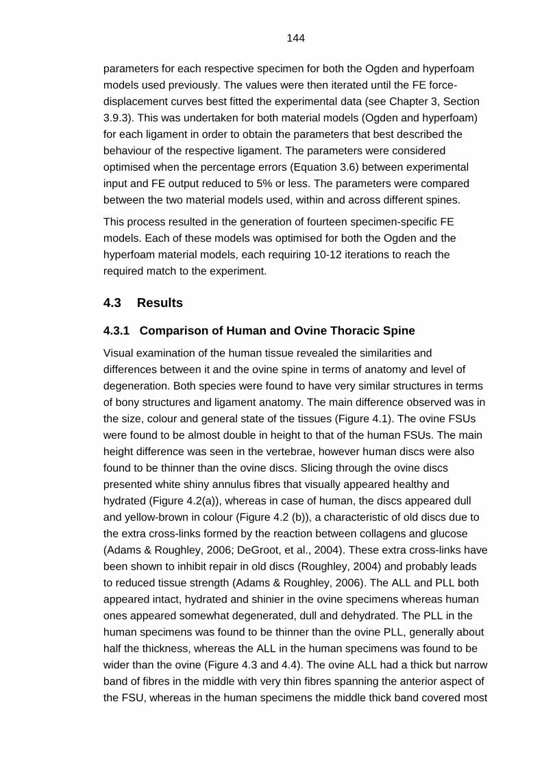
144
parameters for each respective specimen for both the Ogden and hyperfoam
models used previously. The values were then iterated until the FE force-
displacement curves best fitted the experimental data (see Chapter 3, Section
3.9.3). This was undertaken for both material models (Ogden and hyperfoam)
for each ligament in order to obtain the parameters that best described the
behaviour of the respective ligament. The parameters were considered
optimised when the percentage errors (Equation 3.6) between experimental
input and FE output reduced to 5% or less. The parameters were compared
between the two material models used, within and across different spines.
This process resulted in the generation of fourteen specimen-specific FE
models. Each of these models was optimised for both the Ogden and the
hyperfoam material models, each requiring 10-12 iterations to reach the
required match to the experiment.
4.3 Results
4.3.1 Comparison of Human and Ovine Thoracic Spine
Visual examination of the human tissue revealed the similarities and
differences between it and the ovine spine in terms of anatomy and level of
degeneration. Both species were found to have very similar structures in terms
of bony structures and ligament anatomy. The main difference observed was in
the size, colour and general state of the tissues (Figure 4.1). The ovine FSUs
were found to be almost double in height to that of the human FSUs. The main
height difference was seen in the vertebrae, however human discs were also
found to be thinner than the ovine discs. Slicing through the ovine discs
presented white shiny annulus fibres that visually appeared healthy and
hydrated (Figure 4.2(a)), whereas in case of human, the discs appeared dull
and yellow-brown in colour (Figure 4.2 (b)), a characteristic of old discs due to
the extra cross-links formed by the reaction between collagens and glucose
(Adams & Roughley, 2006; DeGroot, et al., 2004). These extra cross-links have
been shown to inhibit repair in old discs (Roughley, 2004) and probably leads
to reduced tissue strength (Adams & Roughley, 2006). The ALL and PLL both
appeared intact, hydrated and shinier in the ovine specimens whereas human
ones appeared somewhat degenerated, dull and dehydrated. The PLL in the
human specimens was found to be thinner than the ovine PLL, generally about
half the thickness, whereas the ALL in the human specimens was found to be
wider than the ovine (Figure 4.3 and 4.4). The ovine ALL had a thick but narrow
band of fibres in the middle with very thin fibres spanning the anterior aspect of
the FSU, whereas in the human specimens the middle thick band covered most

145
of the anterior aspect of the spine. The ovine ligaments were of a distinct
whitish colour which was easier to distinguish from the bone and one could
clearly draw a distinct boundary for all the thick and thin fibres. In contrast, with
the human ligaments, it was hard to draw a clear boundary and the colour was
more of a brown/red nature which was hard to distinguish from the bone and
the surrounding muscles.
Figure 4.1: Examples of the ovine (a) and human (b) cemented FSU illustrating the difference in height (cm).
(a)
(b)

146
Figure 4.2: Examples of the (a) ovine and (b) human disc illustrating the difference in colour and appearance.
Figure 4.3: Photographs of the anterior spine following dissection through the spinal canal showing the differences in the appearance of the (a) ovine and (b) human PLL.
Figure 4.4: Photographs of the anterior spine showing differences in the appearance of (a) ovine and (b) human ALL.
(a) (b)
PLL
(b) (a)
ALL
(b) (a)
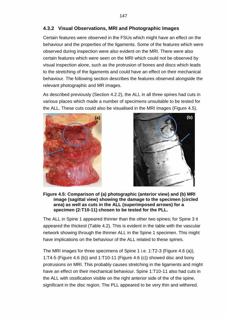
147
4.3.2 Visual Observations, MRI and Photographic Images
Certain features were observed in the FSUs which might have an effect on the
behaviour and the properties of the ligaments. Some of the features which were
observed during inspection were also evident on the MRI. There were also
certain features which were seen on the MRI which could not be observed by
visual inspection alone, such as the protrusion of bones and discs which leads
to the stretching of the ligaments and could have an effect on their mechanical
behaviour. The following section describes the features observed alongside the
relevant photographic and MR images.
As described previously (Section 4.2.2), the ALL in all three spines had cuts in
various places which made a number of specimens unsuitable to be tested for
the ALL. These cuts could also be visualised in the MRI images (Figure 4.5).
Figure 4.5: Comparison of (a) photographic (anterior view) and (b) MRI image (sagittal view) showing the damage to the specimen (circled area) as well as cuts in the ALL (superimposed arrows) for a specimen (2:T10-11) chosen to be tested for the PLL.
The ALL in Spine 1 appeared thinner than the other two spines; for Spine 3 it
appeared the thickest (Table 4.2). This is evident in the table with the vascular
network showing through the thinner ALL in the Spine 1 specimen. This might
have implications on the behaviour of the ALL related to these spines.
The MRI images for three specimens of Spine 1 i.e. 1:T2-3 (Figure 4.6 (a)),
1:T4-5 (Figure 4.6 (b)) and 1:T10-11 (Figure 4.6 (c)) showed disc and bony
protrusions on MRI. This probably causes stretching in the ligaments and might
have an effect on their mechanical behaviour. Spine 1:T10-11 also had cuts in
the ALL with ossification visible on the right anterior side of the of the spine,
significant in the disc region. The PLL appeared to be very thin and withered.
(a) (b)

148
Table 4.2: Differences in the thickness of the ALL across the three spines with white lines drawn over the images of specimens (row 1) to highlight the edges of the ligament while the unaltered images are presented in 2nd row showing that Spine 3 have the thickest and Spine 1 the thinnest ALL.
Spine 1 Spine 2 Spine 3
Figure 4.6: Sagittal view of three specimens of Spine 1 showing bone and disc protrusion in specimen (a) T2-3 and (b) T4-5 leading to stretching of the ALL, and specimen (c) T10-11 showing the fusion of disc and bone on the anterior side as a result of ossification.
(a) (b) (c)

149
Bone compression was also observed in Spine 1:T6-7 (Figure 4.7) which led to
the shortening of the vertebrae on the anterior side, and possible loosening of
the ALL as well as stretching of the PLL.
Figure 4.7: (a) Anterior and (b) top-anterior view of the FSU (Spine 1:T6-7) showing bone compression leading to disc protrusion and bony infusion with the disc.
4.3.3 Mechanical Testing
The load-displacement data obtained for each specimen was processed as
described in Chapter 2, Section 2.5 and the results for the ALL and PLL were
plotted separately (Figure 4.8 and Figure 4.9). It can be seen that all the curves
followed the same basic shape but there was a large difference in gradients.
In order to make a comparison across different specimens, mean bilinear
stiffness values for all the specimens were calculated using the data analysis
method described in Chapter 2, Section 2.5. This gave the initial ‘toe region’
(k1) and final ‘linear region’ (k2) values, which are presented in Table 4.3 and
Table 4.4 respectively. There was a lot of variability evident in both the toe
region and the linear region across the different specimens of both ligaments.
For the ALL, all the specimens belonging to the same spine had similar
gradients i.e. the slopes are closer together for each spine, however no clear
trends were seen for the PLL specimens. The inconsistency between spines
and within specimens could be due to geometric as well as material variability
which will be further explored in the next section. A further comparison of the k2
values with the stiffness values cited in the literature for human spinal
ligaments is presented in Section 4.4.
(b) (a)

150
Figure 4.8: Post-processed load-displacement slopes for all the seven human specimens tested for ALL.
Table 4.3: The ‘toe region’ (k1) and ‘linear region’ (k2) stiffness values calculated by fitting least squares slopes to the post-processed load displacement curves of the ALL specimens. The level and the spine the specimen was obtained from are indicated in the specimen name.
Specimen Stiffness values for ALL (N/mm)
k1 k2
1: T2-3 7 13
1: T4-5 10 19
2: T2-3 34 39
2: T4-5 34 67
2: T8-9 25 55
3: T4-5 80 161
3: T6-7 47 88
Mean ± S.D. 34 ± 25 63 ± 51
0
50
100
150
200
250
300
350
0 0.5 1 1.5 2 2.5 3
Lo
ad
/N
Extension/mm
1: T4-5
1:T2-3
2:T8-9
2:T4-5
2:T2-3
3:T6-7
3:T4-5

151
Figure 4.9: Post-processed load-displacement slopes for all the seven human specimens tested for PLL.
Table 4.4: The ‘toe region’ (k1) and ‘linear region’ (k2) stiffness values calculated by fitting least squares slopes to the post-processed load displacement curves of the PLL. The level and the spine the specimen was obtained from are indicated in the specimen name.
Specimen Stiffness values for PLL (N/mm)
k1 k2
1: T6-7 13 17
1: T10-11 45 72
2: T6-7 16 31
2: T10-11 15 38
3: T2-3 10 55
3: T8-9 14 68
3: T10-11 19 71
Mean ± S.D. 19 ± 12 50 ± 22
-20
0
20
40
60
80
100
120
0 0.5 1 1.5 2 2.5 3
Lo
ad
/N
Extension/mm
1:T10-11
1:T6-7
2:T10-11
2:T6-7
3:T10-11
3:T8-9
3:T2-3

152
4.3.4 FE modelling and material parameter tuning
4.3.4.1 Results using material property data derived under assumptions
of uni-axial stress and uniform geometry
A total of 14 specimen-specific FE models were generated to represent each of
the experimental specimens. Ogden (N=1) and hyperfoam material models
were fitted to the load-displacement data for each ligament using the curve-
fitting algorithm in Abaqus. As explained in Chapter 3, these curve-fitting
algorithms are based on the assumption of a uni-axial stress field and use the
mean cross-sectional area and length. These derived material parameters for
each specimen (i.e. prior to any further parameter optimisation) were then used
as initial values for the material constants in the specimen-specific FE models
of each FSU, and each model was then solved. An example of the resulting
FE-predicted load-displacement curve is shown in Figure 4.10.This output data
was then compared with the corresponding experimental force-displacement
data that was used to derive the material parameter inputs for the respective
ligament. The comparison was computed as percentage difference between
the experimental input and FE output following the procedure described in
Chapter 3, Section 3.9.3, and the results presented in Table 4.5. Again, it was
seen that there were large errors between the experimental and FE data,
following the same outcome as for the ovine specimens presented in Chapter
3. This showed that, as with the ovine specimens, the assumptions used for the
derivation of the material properties in Abaqus (i.e. uniform cross-section and
length, and a uniaxial applied stress (Chapter 3, Section 3.8) were also
incorrect for the human specimens.

153
Figure 4.10: An example of a comparison between the experimental input and resulting FE predicted force-extension behaviour using the Ogden material model for specimen 1:T2-3. The FE material parameters were determined using a mean cross-sectional area and length under the assumption of a uniaxial stress. The disparity in the resulting curves demonstrates that these assumptions were incorrect.
Table 4.5: Percentage difference between experimental input and specimen-specific FE-output using material parameters derived by the in-built Abaqus calibration code assuming mean cross-sectional area and length for all the specimens of ALL and PLL.
Specimen
Percentage Difference (%)
Ogden (N =1) Hyperfoam
ALL
1: T2-3 56.8 45.7
1: T4-5 35.4 12.9
2: T2-3 36.8 19.5
2: T4-5 56.5 36.5
2: T8-9 15.5 20.1
3: T4-5 73.1 65.7
3: T6-7 97.9 49.2
PLL
1: T6-T7 8.5 3.3
1: T10-T11 9.3 16.3
2: T6-T7 28.5 12.2
2: T10-T11 45.0 31.6
3: T2-T3 64.1 34.4
3: T8-T9 35.4 34.5
3: T10-T11 47.2 29.2
0
0.005
0.01
0.015
0.02
0.025
0 2 4 6
Fo
rce(K
N)
Extension (mm)
Experimental Input
FE Output
Mean Percentage difference = 56.8%

154
4.3.4.2 Results following material property calibration
The material parameters were then calibrated to obtain values that produced
the best fit of the specimen-specifc FE model output to the corresponding
experimental curve as described in Section 4.2.3. The example shown in
Figure 4.10 is presented again in Figure 4.11 with the addition of the final post-
optimised FE slope derived from the FE model to illustrate the effect of the
material calibration.
This procedure was applied to each of the specimen-specific models, in each
case iterating the parameters to gain the best fit to the respective experimental
data. The optimised parameters for both ALL and PLL are tabulated in Table
4.6.
Figure 4.11: An example of a comparison of experimental input with pre-optimised and post-optimised FE outputs illustrating the effect of material calibration on Ogden material model for specimen 1:T2-3.
0
0.005
0.01
0.015
0.02
0.025
0 2 4 6
Fo
rce(K
N)
Extension (mm)
ExperimentalInput
FE Output (Pre-Optimisation)
FE Output (Post-Optimisation)

155
Table 4.6: Calibrated material parameters for Ogden (N=1) and hyperfoam material models obtained as a result of the material optimisation procedure undertaken on the specimen-specific FE models by the author.
Specimen Ogden (N=1) Hyperfoam
μ/GPa α D/GPa-1 μ/GPa α
ALL
1: T2-3 7.9E-04 9.4 1170 8.4E-04 5.9
1: T4-5 9.9E-04 7.9 933 9.9E-04 5.3
2: T2-3 1.9E-03 3.8 477 1.9E-03 2.7
2: T4-5 3.0E-03 7.4 308 3.1E-03 4.6
2: T8-9 1.5E-03 9.2 602 1.5E-03 5.9
3: T4-5 4.4E-03 8.3 209 4.6E-03 5.2
3: T6-7 3.9E-03 8.9 235 1.2E-03 5.8
PLL
1: T6-T7 4.1E-03 6.0 225 4.6E-03 4.4
1: T10-T11 1.1E-02 9.7 88 1.1E-02 6.0
2: T6-T7 2.3E-03 9.7 410 1.9E-03 6.6
2: T10-T11 2.5E-03 15.0 369 2.7E-03 8.0
3: T2-T3 7.9E-04 25.1 1167 1.2E-03 9.1
3: T8-T9 1.2E-03 31.3 762 1.8E-03 11.6
3: T10-T11 3.4E-03 24.1 272 3.4E-03 12.9
4.3.5 Comparison of Material Models
As described previously, for the hyperfoam material model, the toe-region of
the load-displacement slope is mainly controlled by μ whereas the curvature is
controlled by α which in turn changes the gradient in the region that
corresponds to the experimental ’linear zone’. Similarly, for the Ogden (N=1)
material model, the toe region is controlled by both μ and D whereas the
curvature is controlled by α. But since μ is directly related to D for a given
Poisson’s ratio as assumed here (Equation 3.4, Chapter 3), altering either
would automatically change the value of the other. Hence, here only the effects
of μ will be discussed when considering the toe region for the Ogden (N=1)
material model.
In addition, it was found that the values for μ and α for the two material models
were relatively well correlated for both the ALL and PLL, as shown in Figure
4.12 and Figure 4.13. Hence, only the Ogden (N=1) material model will be
discussed in the subsequent comparisons between coefficients and across
spines and levels.

156
Figure 4.12: Graphical comparison of the material coefficient μ for both (a) ALL and (b) PLL derived using the two material models, showing that they are very similar hence either material model could be used for further analysis.
0.0E+00
1.0E-03
2.0E-03
3.0E-03
4.0E-03
5.0E-03
6.0E-03
0.0E+00 1.0E-03 2.0E-03 3.0E-03 4.0E-03 5.0E-03
Ogden (
N=
1)
Hyperfoam
0.0E+00
2.0E-03
4.0E-03
6.0E-03
8.0E-03
1.0E-02
1.2E-02
0.0E+00 2.0E-03 4.0E-03 6.0E-03 8.0E-03 1.0E-02 1.2E-02
Ogden (
N=
1)
Hyperfoam
(b)
(a)

157
Figure 4.13: Graphical comparison of the material coefficient α for both (a) ALL and (b) PLL derived using the two material models showing that they are related hence either material model could be used for further analysis.
4.3.6 Comparison between Coefficients
The material coefficients for Ogden (N=1) were plotted against each other
(Figure 4.14) to examine if there was any relationship between the two. The
graph illustrates that no clear relationship between the two can be drawn,
hence both coefficients will be discussed in the following sections.
0.0
1.0
2.0
3.0
4.0
5.0
6.0
7.0
8.0
9.0
10.0
0.0 1.0 2.0 3.0 4.0 5.0 6.0 7.0
Ogden (
N=
1)
Hyperfoam
0.0
5.0
10.0
15.0
20.0
25.0
30.0
35.0
0.0 2.0 4.0 6.0 8.0 10.0 12.0 14.0
Ogden (
N=
1)
Hyperfoam
(a)
(b)

158
Figure 4.14: Material coefficients plotted against each other for Ogden (N=1) material model. The figure illustrates that both coefficients are not related and hence both have to be discussed in further analysis.
4.3.7 Comparison by spine and by level
The material coefficients for each ligament group were plotted in groups of their
respective spine (Figure 4.15 and Figure 4.16) and also by level (Figure 4.17
and Figure 4.18) to visualise the differences. Although there is not enough data
to perform a statistical analysis, however, from the graphs, there was a large
spread in values of both alpha and µ across the PLL and ALL. There were no
clear trends for each ligament group; for example, the μ value for the ALL was
highest in Spine 3 whereas for the PLL, it was highest in Spine 1. Similarly, the
α value for the ALL did not vary much across different spines while for the PLL,
it was highest in Spine 3. In some cases, there was more difference between
spines than between levels (see Figure 4.15a and Figure 4.16b) and there
were no clear trends seen between levels (Figure 4.17 and Figure 4.18).
0.0
5.0
10.0
15.0
20.0
25.0
30.0
35.0
0.0E+00 2.0E-03 4.0E-03 6.0E-03 8.0E-03 1.0E-02 1.2E-02
α
μ (GPa)
ALL
PLL

159
Figure 4.15: Comparison of μ for Ogden (N=1) for (a) ALL and (b) PLL specimens by spine (left to right is from upper to lower levels). In the case of the ALL, there were bigger differences between spines than within each spine.
0.0E+00
5.0E-04
1.0E-03
1.5E-03
2.0E-03
2.5E-03
3.0E-03
3.5E-03
4.0E-03
4.5E-03
5.0E-03
1 2 3
µ (
GP
a)
Spine
Series1
Series2
Series3
0
0.002
0.004
0.006
0.008
0.01
0.012
1 2 3
µ (
GP
a)
Spine
Series1
Series2
Series3
(a)
(b)
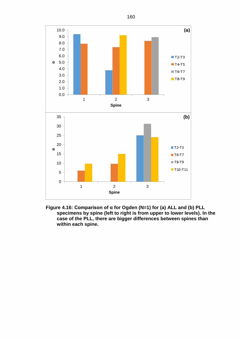
160
Figure 4.16: Comparison of α for Ogden (N=1) for (a) ALL and (b) PLL specimens by spine (left to right is from upper to lower levels). In the case of the PLL, there are bigger differences between spines than within each spine.
0.0
1.0
2.0
3.0
4.0
5.0
6.0
7.0
8.0
9.0
10.0
1 2 3
α
Spine
Series1
Series2
Series3
0
5
10
15
20
25
30
35
1 2 3
α
Spine
Series1
Series2
Series3
(b)
(a)

161
Figure 4.17: Comparison of μ for Ogden (N=1) for (a) ALL and (b) PLL specimens by level showing big differences across individuals but no clear trends between levels are evident.
0.0E+00
5.0E-04
1.0E-03
1.5E-03
2.0E-03
2.5E-03
3.0E-03
3.5E-03
4.0E-03
4.5E-03
5.0E-03
T2-T3 T4-T5 T6-T7 T8-T9
μ/G
Pa
Spine Section
Spine 1
Spine 2
Spine 3
0.0E+00
2.0E-03
4.0E-03
6.0E-03
8.0E-03
1.0E-02
1.2E-02
T2-T3 T6-T7 T8-T9 T10-T11
μ/G
Pa
Spine Section
Spine 1
Spine 2
Spine 3
(b)
(a)

162
Figure 4.18: comparison of α for Ogden (N=1) for (a) ALL and (b) PLL specimens by level showing big differences across individuals in the case of PLL but no clear trends between levels are evident.
4.3.8 Comparison with other computational data
To the authors knowledge no study has published hyperelastic material data, in
terms of material parameters, for spinal ligaments hence a direct comparison
with the material parameters obtained as a result of this study is not possible. It
is, however, possible to compare the Young’s modulus values used in other
studies with an equivalent modulus at a given strain derived from the
hyperelastic equations used here.
Equation 3.5 (Chapter 3) was differentiated to obtain an expression for the
stress-strain gradient to make comparisons to the Young’s modulus
documented in other studies (Equation 4.1).
𝑑𝑆/𝑑𝜖 = 2𝜇
𝛼[ ((
𝛼−2
2) (2𝜖 + 1)
𝛼−4
2 ) − (2 (−𝛼
4− 1) (2𝜖 + 1)−
𝛼
4−2)] [eq. 4.1]
0.0
1.0
2.0
3.0
4.0
5.0
6.0
7.0
8.0
9.0
10.0
T2-T3 T4-T5 T6-T7 T8-T9
α
Spine Section
Spine 1
Spine 2
Spine 3
0.0
5.0
10.0
15.0
20.0
25.0
30.0
35.0
T2-T3 T6-T7 T8-T9 T10-T11
α
Spine Section
Spine 1
Spine 2
Spine 3
(b)
(a)

163
The majority of computational modelling studies have represented the
behaviour of the ligaments up until the end of their linear regions with some
using only a single linear region at all strains (Chapter 1, Section 1.2.6). To
make comparisons with the literature, the strain at the end of linear region was
used. This provided a comparison at the highest strain the ligaments would
likely experience in vivo. Chazal et al. (1985) determined strain at the end of
linear region for the ALL as 12% while a value of 20% strain has been
documented for PLL to be within the physiological range and at the end of
linear region (Ruberte et al., 2009)). These values were used in Eq.4.1 along
with the material parameters for each individual ligament, and the resulting
stress-strain gradients are presented in Tables 4.7 and 4.8. The average
gradients for both ALL and PLL was also deduced and was compared with the
Young’s Modulus data from the simple computational models (Chapter 1, Table
1.9) in the linear range. The comparisons are presented in Figure 4.19 & Figure
4.20.
Table 4.7: Estimated values of the stress-strain gradient at 12% strain (E) from the material parameters for all the specimens of ALL (n=7).
Specimen µ (MPa) α E (MPa)
1: T2-T3 7.9E-04 9.4 1.6
1: T4-T5 9.9E-04 7.9 1.8
2: T2-T3 1.9E-03 3.8 3.0
2: T4-T5 3.0E-03 7.4 5.2
2: T8-T9 1.5E-03 9.2 3.0
3: T4-T5 4.4E-03 8.3 8.1
3: T6-T7 3.9E-03 8.9 7.5
Average ± S.D. 4.3 ± 2.7

164
Table 4.8: Estimated values of the stress-strain gradient at 20% strain (E) from the material parameters for all the specimens of PLL (n=7).
Specimen µ (MPa) α E (MPa)
1: T6-T7 4.1E-03 6.0 5.9
1: T10-T11 1.1E-02 9.7 25.3
2: T6-T7 2.3E-03 9.7 5.4
2: T10-T11 2.5E-03 15.0 14.3
3: T2-T3 7.9E-04 25.1 25.3
3: T8-T9 1.2E-03 31.3 111.6
3: T10-T11 3.4E-03 24.1 91.6
Average ± S.D.
39.9 ± 43.3
Figure 4.19: Comparison of Young's modulus (E) between the average value of ALL from the current study and the data cited by computational studies. *others include; Lee & Teo (2005), Polikeit et al. (2003), Lee & Teo (2004), Sylvestre et al. (2007), Bowden et al. (2008), Tsuang et al. (2009), Moramarco et al. (2010)
0
5
10
15
20
25
30
E (
MP
a)
This Study
Goel et al. (1995) &others*
Ruberte et al. (2009)
Hortin & Bowden (2016)

165
Figure 4.20: Comparison of Young's modulus (E) between the average value of PLL from the current study and the data cited by computational studies. *others include; Lee & Teo (2005), Tsuang et al. (2009) **others include; Lee & Teo (2004), Sylvestre et al. (2007), Bowden et al. (2008)
4.4 Discussion
4.4.1 Discussion of Experimental Results and Visual Observations
This chapter presented the procedures adapted to characterise the human ALL
and PLL. The results alongside visual observations and possible causes is
discussed below. The testing was carried out on thoracic regions of human
cadaveric spines and the results were presented as load-displacement curves
for each ligament (Figure 4.8 and Figure 4.9). The curves all followed the same
basic shape but there were large differences in the gradients. Both Figures 4.8
and 4.9 show that there were generally larger differences between the spines
than within each spine because the curves for each spine mostly lie next to
each other. There was one outlier to these observations: specimen T10-11
from Spine 1 showed a considerably higher stiffness than all other PLL
specimens. This specimen was found to have anterior ossification as well as
big cuts in the ALL and its MRI scans showed bony protrusions into the disc
space (see Figure 4.6 (C)). This would suggest that the two vertebrae were
self-fusing together and could potentially imply that the attached ligament on
the anterior side i.e. the ALL had become redundant and was wasting away.
The PLL on the other hand could have been subjected to greater loads as the
hardening on the anterior side might result in an anterior pivoting under flexion
and greater stretch of the posterior side (see Figure 4.21), and hence the PLL
-10
0
10
20
30
40
50
60
70
80
90
E (
MP
a)
This Study
Goel et al. (1995) & others*
Ruberte et al. (2009)
Hortin & Bowden (2016)
Polikeit et al. (2003) &others**

166
has to be stiffer to compensate. The fusion of vertebrae have been shown to be
related to many underlying conditions, including degeneration of discs as a
result of old age or trauma. Fusion due to both organic means (Benzel, 2012)
or as a result of surgery (Srinivas, et al., 2016; Lee & Choi, 2015), has been
shown to result in regions of increased stress and strain in segments adjacent
to the fused segments. This indicates a change in the load distribution following
fusion, and since ligaments play a role in providing stability to the spine
alongside facets (Sharma, et al., 1995) and discs, an imbalance due to
changing any of the stabilising structures will alter the role of the other two (Ng,
et al., 2003). Moreover, anterior ossification can be related to diseases such as
the idiopathic skeletal hyperostosis (Resnick, et al., 1975) which mainly affects
the thoracic spine, or ankylosing spinal hyperostosis (Forestier & Lagier, 1971).
While a specific diagnosis from the evidence seen for Spine 1 is not possible, it
is important to note that these diseases are known to be associated with spinal
enthesopathy, a phenomenon related to ossification of paraspinal ligaments
(Nakhoda & Greene, 2016). If the anterior ossification observed in the Spine 1
specimens is associated with any of the diseases mentioned above, then the
ossification of the PLL is also quite possible, which would result in an increased
stiffness. This could potentially be another reason for the stiffer PLL.
Figure 4.21: A schematic illustration of anterior flexion in healthy FSU and in degenerated FSU due to anterior ossification. (a) illustrates an FSU of an healthy individual in a resting state with posterior (P) and anterior (A) side labelled; (b) illustrates the same healthy FSU when the individual bends forward; there would be anterior disc compression with the centre of rotation located towards the middle of the disc; (c) illustrates an individual with anterior ossification that leads to anterior pivoting of the vertebra during forward flexion, resulting in greater stretching of the structures at the posterior.
The anterior ossification that leads to bone and disc protrusions is also evident
in two other specimens of Spine 1, which were both used for testing the ALL.
Both these specimens show very low stiffness values and the ALL was thinner
P A
Vertebra
Disc
Vertebra
(a) (c) (b)

167
than in the other two spines (e.g. Table 4.2), which would corroborate the
theory stated above about the ALL having become redundant.
The tables of bilinear stiffness (Table 4.3 and 4.4) show that the value of k2 is
generally double or higher than the k1 value, however for the Spine 1
specimens, this does not hold true and there is a little difference between the
k1 and k2 values. This could be due to the ossification and bony protrusions
that led to the over-stretching of the ligament, which could potentially cause the
ligaments to operate in the linear region with the collagen fibres already
straightened. In the ALL, this is likely due to the over exertion caused by bone
protrusions anteriorly, and to PLL, due to the overextension and/or secondary-
ossification discussed above. This is especially true in the case of Spine 1:T6-7
(see Figure 4.7) whereby bone compression led to misalignment of spine and
PLL potentially stretched beyond its normal limits to keep the spine in place.
4.4.2 Discussion of Finite Element Modelling
The FE modelling of ligaments provides further evidence for the idea previously
established in Chapter 3 (see Section 3.8) that the assumption of a uniform
mean cross- sectional area and length, and a resulting uniaxial stress state,
cannot be used to derive the properties of the ligament accurately. As shown in
Table 4.5, using these assumptions led to large differences between
experimental output and FE output. There could be a number of other factors
causing discrepancies between the FE predictions and experimental data, such
as variations in dimensions and boundary conditions, or errors due to the mesh
size used (Chapter 3, Section 3.6.1)., however, these discrepancies will be
small as efforts were made to ensure that the geometry used and boundary
conditions applied were realistic (Chapter 3). Moreover, it was ensured that the
mesh size used was defined by the optimum mesh size established in Chapter
3, Section 3.6.1.3. Therefore it seems likely the majority of the difference is due
to the assumption of uniform geometry and uniaxial stress.
The optimisation procedure undertaken subsequently resulted in the final FE
outputs being very close to the experimental outputs, with the accepted
percentage difference of 5% or less between the two outputs being achieved in
all cases. To the best of our knowledge, this is the first FE study showing that a
uniform cross-sectional area and length cannot be used to represent the
accurate behaviour of ligaments. However, in FE modelling of knee ligaments,
a comparison between springs and geometrically accurate ligaments has been
carried out (Beidokhti, et al., 2017). They built two models; one with one-
dimensional spring elements, as a way of simplifying the geometry, and the
other with three-dimensional continuum elements based on segmentation and

168
found more accurate contact outcome variables with the continuum modelling
approach. Although the springs used in that study were not directly comparable
to the uniform geometry assumptions used here, the study provides further
evidence of the importance of modelling geometrically accurate ligaments.
4.4.3 Comparison and Analysis of Material Parameters
The hyperfoam or Ogden model optimised values provided a numerical way of
capturing the difference between the experimental curves, as the two
coefficients influence different parts of the curve; µ influences the toe-region
whereas α influences the curvature, as previously described in Chapter 3
(Section 3.9.2 & 3.9.3). If the slope has greater curvature (that is, has a higher
exponential), it is due to the α value being higher and if its initial gradient is
higher, then the µ value is higher. Hence, one can deduce the relative shape of
the load-displacement slope for a specimen from the material coefficients and
vice versa. For example, the values of µ for the ALL specimens for Spine 3 are
larger than for the other two spines (see Figure 4.15) because the toe region of
these specimens has a higher gradient (see Figure 4.8). Whereas the α value
for all these specimens are very similar because the curvature across all these
specimens is very similar in what would be classed as the ‘linear zone’ of the
slope. The main difference in α is seen in specimen 2:T2-3 (Figure 4.16),
displaying the lowest value, because it has a very low curvature and maintains
a low gradient in the ‘linear zone’ (Figure 4.8). In the case of the PLL, the value
of µ is highest for specimens of Spine 1 (See Figure 4.15) because the
specimens have higher toe region than the others, especially specimen 1:T10-
11 (Figure 4.17) which was steeper than all the other PLL specimens (Figure
4.9). Similarly, the α value for Spine 3, in the case of the PLL, has higher
values than the other two spines because the curvature of the load-
displacement slopes of these specimens is greater than the others.
It is important to remember that the models used are all phenomenological
hence the resulting material coefficients do not have direct physical meaning as
described previously (Chapter 1, Section1.2.7; Chapter 3, Section 3.10).
However, as described, their effect is seen in different parts of the load-
displacement curve. Since we know that different components of the ligament
e.g. elastin content, collagen content, amount of collagen crimping etc. affect
the load-displacement slope (Chapter 1, Section 1.2.4.1), some comparisons
between the tissue composition and structure and the two variables can be
made but it must be noted that it is not a one-to-one mapping because there
are only two material variables as opposed to multiple tissue variables. Based
on the above, it could be hypothesised that the collagen fibres straightening out

169
and taking the load dominates the behaviour of α since collagen dominates at
higher strains once it straightens out, whereas for µ, the elastin is taking more
of the load as it dominates at low strains. However, there is no clear distinction
between the two variables and their relevance to the tissue structures. Even if
we just consider the collagen, there are several different factors that can affect
the shape of the slope such as the amount of collagen will affect the overall
gradient once all the fibres uncrimp, while the variability in crimping will affect
how quickly the gradient changes i.e. if all the crimps straighten at the same
strain, then there would be a very sudden change in gradient, compared to a
more gradual curve if different crimps straightened at different strains. Since
the best exponential fit accommodates both of these factors, they cannot be
differentiated. For example, it was observed that Spine 3 specimens (red
curves in the Figure 4.8 and Figure 4.9) had the highest stiffness overall for
both ligaments. This spine was also found to have the highest α value in the
case of PLL than the other two spines. The α value for ALL for this spine is in
the higher spectrum compared to other ALL specimens. If the microstructure of
these ligaments is influenced by the material parameters in the same manner
as described above, then the ligaments of this spine, especially the PLL,
probably have either a higher amount of collagen fibres and/or the fibres are
stiffer once un-crimped. If the same also holds true for Spine 1 which was
found to have highest µ for PLL specimens but lowest for ALL, then the PLL
would have adapted to the anterior ossification observed in these specimens,
as discussed above, and have higher amount of collagen fibres or the fibres
are more crimped. Or else if the PLL has not adapted and is stiff due to
secondary ossification, as described above, then the higher µ value is
influenced by the ossified structure. ALL specimens for Spine 1, on the other
hand, with lowest µ values, also have the lowest stiffness values supporting the
visual observation about the ligaments becoming redundant due to anterior
ossification of the disc. So the collagen fibres have either stretched beyond
their capacity and are working in the liner region or the amount of elastin in
these ligaments have reduced immensely. This also shows the differences
amongst individual spines due to a disease or inherent difference in the tissue
microstructure. Such speculations can only be supported by a histological
analysis, which is beyond the scope of this study. This helps illustrate the point
about the material models being phenomenological, i.e. they do not have any
physical relevance and purely simulate the mechanical behaviour. The models
might give an indication about the structural relevance in a healthy state but
would not be able to predict true relevance in a diseased state such as
ossification.

170
The values of the material coefficient µ obtained for all the specimens are very
similar between the two material models (see Table 4.6). The values for α
however are different but are mostly of the same order of magnitude in both
cases (see Table 4.6). Graphical representation of this is presented in Figure
4.12 and 4.13. However, for both models, the coefficients are not related to
each other (Figure 4.14) so it is not possible to derive one from the other. This
is not surprising given that different material factors affect each coefficient (as
discussed previously), and would not necessarily vary in the same way from
specimen to specimen.
4.4.4 Variability across Individual Spines and Spinal Levels
As with the stiffness values, a comparison of material coefficients across the
three spines (Figure 4.15 and Figure 4.16) and across different levels (Figure
4.17 and Figure 4.18) showed that there are bigger differences between spines
than there are between levels. The differences between spines is discussed in
detail above in relation to the material parameters. No clear trends are evident
between levels and one cannot comment if moving along the length of the
spine has any significant effect on the material properties of the ligament. This
might be because this study is restricted to thoracic region where the spine is
held in place and the motions are restricted by the rib cage, hence the
differences along the length are not very evident. If the study were performed
over a longer length with the inclusion of either the cervical or the lumbar region
where there are greater differences in loading and range of motion (Chapter 2,
Section 2.7.1), then more trends may have been evident. In the lumbar spine
for example, where there is greater curvature, there will be differences from
one vertebrae to another in the articulation and because the motions are not
restricted. This has been shown in a recent study by Putzer et al. (2016) who
found that the lumbar spine kinematics have a trend towards increased lower
lumbar flexion.
The big differences observed between the three spines show that each
individual is different to the others and places emphasis on the importance of
specimen-specific modelling. Although it is difficult to determine the exact
properties of each ligament for each individual without having to perform an
elaborate study like this, however, the state of the spine and the tissue as
observed through an MRI scan of the individual can give an indication of what
category it falls under. For example, physical inspection of Spine 1 revealed
right anterior ossification. This was seen on MRI scan as bone and disc
protrusions showing that the ligaments are stretched in those regions. Even if
the ligaments had adapted and were no longer under a greater stress due to

171
this increased stretch around the protrusions. When the disc was dissected
during the testing, this removed more strain than in the normal disc state.
Therefore, regardless of where on the stress-strain curve the ALL usually
operates (in a stretched or adapted state), the start of the test would have been
moved further to the left (towards a lower strain) than normal, which could
explain why the specimens tested for the ALL showed a lower stiffness than the
specimens from other spines (Table 4.3). The PLL in these regions would also
have to be stiffer as discussed above. Specimen 1:T10-11 displays this higher
stiffness in the PLL, however, specimen 1:T6-7 displays quite a low stiffness
comparatively (Table 4.4), assuming the above hypothesis holds true. This can
be attributed to the bone compression evident in this specimen (Figure 4.7)
which might have already caused damage to the PLL hence the low stiffness.
This shows that although some evidence on the ligament properties can be
gleaned from the MRI, it may not always be possible to predict likely properties
because of damage or overstretching that is not visible.
4.4.5 Comparison with Published Human Data
The main aim of this section was not only to characterise the human spinal
ligaments but also to compare the data obtained with the published human
data. To the author’s knowledge, no data has been published on the material
parameters of spinal ligaments, which could be directly compared with the
material coefficients obtained in this study. As previously discussed in Chapter
1 (Section 1.2.7), hyperelastic material models have been used to model other
joints and ligaments in the human body however, a comparison with the
material parameters used in those studies would not be appropriate since large
differences are observed even between the ALL and PLL. For this reason, it
was only possible to compare an equivalent modulus at a given strain from this
study with Young’s modulus values cited in previous computational modelling
studies. (Section 4.3.8). The comparison shows that the Young’s modulus for
the ALL averaged from this study is lower than the values used by
computational modelling researchers whereas the value for PLL lies
approximately in the middle of what is used by these researchers. The majority
of these computational studies used the experimental data cited in literature to
work out the material properties for ligaments. Some refer to other
computational studies as a reference, and following the trail leads to the same
experimental studies as the others. The differences observed are due to the
differences in the experimental procedures used to generate the data in
respective studies. The study by Pintar et al. (1992) was found to be the
original source of data for most studies (Goel et al. (1995), Lee & Teo (2005),
Polikeit et al. (2003), Lee & Teo (2004), Sylvestre et al. (2007), Bowden et al.

172
(2008), Ruberte et al. (2009), and Tsuang et al. (2009)). The other sources of
data cited were traced back to the study by Chazal et al. (1985) (Polikeit et al.
(2003), Lee & Teo (2004), Sylvestre et al. (2007), Hortin & Bowden et al.
(2016)). The experimental studies cited stiffness values which were
manipulated by the researchers alongside the geometric properties i.e. cross-
sectional area and length, to derive the Young’s modulus.
Some studies used different sources for obtaining the data for different
ligaments e.g. Polikeit et al. (2003) used a Young’s modulus of 20 MPa for the
ALL from Pintar et al. (1992), but 70 MPa for the ALL which was derived from
Chazal et al (1985). Some studies referenced back to the same experimental
study but cited different modulus values. For example, Ruberte et al. (2009)
cited 15.6 MPa for the ALL whereas Polikeit et al. (2003) cited 20 MPa,
although both referenced back Pinter et al. (1992). While these differences may
be due to the difference in the level of FSU used, there is a lot of ambiguity in
how the Young’s modulus values were derived. Regardless of how the modulus
values were derived, the values used previously for the ALL are all
considerably higher than the stress-strain gradient derived from the steepest
physiological portion of the stress-strain curve in any of the specimens tested
here. This could be because of the differences in specimens, spinal levels etc.
as discussed in detail below, but it may also suggest that the modulus has
previously been overestimated. The assumptions made about uniform
geometry to convert the published stiffness into a Young’s modulus could be
likely reason for this overestimation, as is shown by this study. Nevertheless, it
is difficult to know whether any overestimation of the ALL properties would
have changed the study outcomes, because no sensitivity tests were
undertaken.
In order to make direct comparisons between the original experimental data
and the current study, the two most cited experimental studies by the
computational modellers i.e. Chazal et al. (1985) and Pintar et al. (1992) were
also analysed. The study by Chazal et al. (1985) could not be compared to for
two reasons; they did not publish stiffness data to allow us to make direct
comparisons, and, they tested the ligaments individually as opposed to keeping
them in situ (current study) which has been shown to bring about differences in
the results as discussed previously in detail in Section 1.2.5.4.
Pintar et al. used the data from Myklebust et al. (1988) who performed a study
on 41 fresh human male cadavers with a mean age of 67 years (ranging from
30-89 years). Whole ligament stiffness values were cited, but only in terms of
k2 as the toe region was neglected. The authors tested ligaments at each level

173
in isolation, in situ, and all the supporting structures except the ligaments to be
evaluated were sectioned through. Pintar et al. (1992) analysed the data on
specimens of the lumbar region of the spines from the above study and
presented the mean stiffness (slope of the least-squares fit line) values of the
linear portion of the force-deformation curve. The values published for ALL (33
± 15.7 N/mm; n=25) and PLL (20.4 ± 11.9 N/mm; n=21) were both found to be
less stiff than the ones obtained for human ALL (63 ± 51 N/mm) and PLL (50 ±
22 N/mm) in this study. An un-paired t-test was carried out to see if the stiffness
values were significantly different between the two studies for both ALL and
PLL. The data was assumed to meet the requirements for an unpaired t-test,
i.e. that there were no outliers and the data was normally distributed, since it
was not possible to access the raw data from this study. It was found that there
was a significant difference (P<0.05) between the means of stiffness values of
ALL for the two studies whereas no significant difference was found between
the means of the stiffness values obtained for the PLL from the two studies. It is
important to note that the specimens are not fully independent, as several
specimens came from the same spine.
There could be a number of reasons for the differences in the mean stiffness
values including the testing regime, the regions tested (thoracic or lumbar), the
tissue storage method and the age, gender and fitness level of individual, which
are each discussed below.
Regional differences
Our study was performed on the thoracic region whereas the published data
was obtained from lumbar region, therefore, the differences in the stiffness
might be due to the difference in the regions. To author’s knowledge no study is
published on intra-individual differences between spinal ligaments mechanics
from different regions. However, Weiler et al. (2012) performed a study on
human intervertebral discs (IVD) in order to analyse the amount of
degenerative changes in different spine levels in humans from different ages.
They found the cervical and thoracic disc specimens showed significantly less
degenerative changes compared to the lumbar region (Weiler, et al., 2012). If
the same is true for the spinal ligaments then this could also explain some of
the stiffness differences between the two studies. Some differences in ALL
structure at varying regions of the vertebral column were illustrated by Bogduk
(1997) and Bannister et al. (1996). Bogduk (1997) found that the ALL was not
associated with any of the prevertebral muscles in the thoracic region and
therefore, stood alone. This shows functional differences in the ligament over
the length of spine. Bannister et al. (1996) reported that ALL is thicker and

174
narrower in the thoracic region as compared to the other regions, and broadens
as it travels caudally. These differences likely alter the cross sectional area and
hence stiffness if the material properties remain constant. Further comparison
of dimensions in different regions is hampered by the huge differences in the
values reported (see Chapter 1, Table 1.9) depending on the method of
measurement used, as described previously in Chapter 1, Section 1.2.5.1.1
and Section 1.2.6.7.
Age differences
The specimens in this study were obtained from cadavers with mean age of 86
years, which is higher than the mean age (67 years) of the published data. This
could be another likely reason for differences seen in stiffness as the
mechanical properties of the spine have been found to deteriorate with
increasing age (Nachemson & Evans, 1968; Tkaczuk, 1968; Neumann, et al.,
1994; Pintar, et al., 1998; Neumann, et al., 1992; Iida, et al., 2002). The
ligament properties have been shown to correlate with the bone mineral
content (Neumann, et al., 1994; Pintar, et al., 1998) which is known to decline
after the age of 50 due to the onset of osteoporosis (Kanis, et al., 1994)
therefore a change in their mechanical properties is inevitable. Moreover, the
ligament properties are closely related to the collagen content present which
decreases with age, resulting in a decline in material properties such as their
strength and the ability to withstand deformation (Cowin & Doty, 2007).
Tkaczuk, (1968) carried out testing on lumbar ALL and PLL and found a
decrease in failure force, stress, and elongation with increasing age.
Nachemson et al., (1968) also found the modulus of elasticity and failure stress
in lumbar LF to go down by a factor of four between the ages of 20 to 80 years.
A similar aging effect on ligament failure stress was observed by Chazal et al.,
(1985). This shows that with increasing age both the elasticity and the collagen
content decreases which ultimately will result in a decreased elongation and
failure force. However, these studies were carried out on sections of ligaments
as opposed to our study, hence evaluating the material properties but not the
total stiffness of the ligaments. The stiffness is related to both the modulus as
well as the dimensions, so although the modulus was shown to decrease in
these studies there might be counteracting changes in geometry (e.g. ligament
thickening) which will give an overall increase in stiffness with age. Neumann
et al., (1994) has shown greater effects of increased cadaver age, and
decreased vertebral mineral content on isolated lumbar ALL specimens at slow
elongation rates with stiffness varying by as much as 5 times across regions.
They found increased stiffness at mid-substance whereas a decreased
stiffness was found at the insertion point of the ligament compared to younger

175
specimens. This shows that aging affects different regions of ligaments in
different ways (Neumann, et al., 1994). If slow elongation rates are used, the
mid-substance of the ligaments is exploited whereas the low stiffness and
failure at the insertion points at faster loading rate might be a result of
mechanical integrity of the Sharpey's fibre insertions or the underlying layer of
bone, or both, during aging as hypothesised by Neumann et al. (1994 (Cowin &
Doty, 2007)). This might explain why studies carried at a comparatively higher
loading rate to this study (Myklebust, et al., 1988; Iida, et al., 2002) have found
the elastic stiffness of ligaments to decrease with increasing age; if there was a
progressive pulling out of the Sharpey’s fibres even before failure.
Differences in testing regimes
The testing regimes of both studies; this study and the study by Pintar et al.
(1992), were the same in terms of the ligaments being tested in situ and all the
supporting structures except the ligament to be evaluated were sectioned.
However, the loading rates in both cases were very different with Pintar et al.
(1992) using a faster rate of 600 mm/min compared to 1 mm/min used in this
study. As described previously (Chapter 2, Section 2.7), an increase in loading
rate has been shown to increase the stiffness in cervical spinal ligaments in
similar isolated bone-ligament-bone samples (Butler, et al., 1988; Mattucci, et
al., 2012; Trajkovski, et al., 2014). If the same is true for the lumbar spine, then
the published stiffness by Pintar et al. (1992) would be lower if the tests were to
be carried out at a slower loading rate of 1 mm/min. However, Pintar et al.
(1998) carried out compressive loading on whole cervical spines and found that
the loading rate effects decreased with increasing age. The interaction between
loading rate and age was thought to be attributed to the degradation of bone
with age since most failures occurred in the bone. This may also affect ligament
properties, as ALL and PLL properties have been shown to correlate with bone
mineral content in the vertebrae, which goes down with age (Neumann, et al.,
1994) as discussed previously, and so the loading rate effect might not make a
significant difference to the values obtained for elderly specimens because the
aging effects overrides other effects.
Differences due to storage method
The published data was obtained from fresh specimens whereas the data in
this study was obtained from frozen specimens that have gone through a
number of freeze-thaw cycles before the testing. Freezing specimens on the
day of retrieval with subsequent dissection and testing on a later day has been
shown to not affect the behaviour of ligaments adversely (Chapter 1, Section
1.2.5.4). However, since the specimens in this study had unavoidably gone

176
through a number of freeze-thaw cycles, despite efforts to reduce water loss,
this could have caused dehydration of the tissue hence resulting in a stiffening
of the ligaments.
The large standard deviations in this study are an indication of just how variable
the tissue is from one individual to another. It is therefore quite likely that these
two studies simply represent different samples taken from the natural range
across different spinal levels and age distributions, and hence both the studies
are equally valid.
The differences in stiffness values due to biological variability and aging effects
are an inevitable consequence of cadaveric research but the differences due to
testing regimes can be controlled. Hence a comparison of the human and ovine
data obtained as a result of testing carried out in the same manner is
conducted in Chapter 5.
4.4.6 Conclusion
In conclusion, this chapter has presented new data on the behaviour of the
thoracic longitudinal ligaments, including parameters for material models that
represent its non-linear behaviour for the first time. It is apparent that these
properties are highly variable from one person to another, which poses
challenges for representing the behaviour in finite element models of the spine.

177
Chapter 5
Discussion
5.1 Introduction
This chapter brings together all the key results obtained from this work and
discusses their meaning in a wider context. The limitations of the work are also
discussed, followed by some suggestions for future work. The chapter ends
with final concluding statements to emphasise the key points and the
significance of this work.
Overall from this work, a new method has been developed to mechanically
characterise the spinal ligaments using a combined experimental and
computational approach. The method was successfully applied to the
longitudinal ligaments, namely the anterior longitudinal ligament (ALL) and
posterior longitudinal ligament (PLL), but has the potential to be replicated on
the other ligaments of the spine. The method was developed on ovine spines
and was successfully applied to human spines resulting in new data on the
mechanical properties of both ovine and human ALL and PLL.
In the literature (Chapter 1, Section 1.2.6), the spinal ligaments have been
characterised either by their overall mechanical behaviour (i.e. stiffness), or by
the underlying material behaviour (most commonly measured through a
Young’s modulus). The stiffness is useful in understanding the relative effects
of the different ligaments, such as in the larger scale models of the spine where
ligaments are represented by springs or truss elements. Whereas the material
properties are useful in understanding the effects of differences in the material
composition of the ligaments, and in FE models where the ligaments are
represented as solid structures.
Both the ovine and human specimens were found to have stiffness values
higher than those cited in literature (see Chapters 2 and 4). A comparison of
both human and ovine stiffness values in relation to each other is presented in
the next section. Moreover, a poor agreement was found between the material
parameters derived from FE models and the initial values derived by assuming
uniaxial behaviour, that is, assuming uniform cross-sectional area and length
(see Chapters 3 and 4). The material parameter values for the human spine
were found to be more consistent within each spine than between spines (see
Chapter 4). The material parameters obtained for both human and ovine
specimens are also compared in the following section.

178
5.2 Comparison of the stiffness values for human and ovine
longitudinal ligaments
It was clear from the experimental data that both ovine (Chapter 2) and human
ligaments (Chapter 4) exhibited a non-linear load-displacement relationship.
Therefore, in order to make comparisons, a bi-linear model was employed as
had been used previously in the literature (Chapter 1, Section 1.2.6). Figure
5.1 shows a comparison of the toe-region (k1) and linear-region (k2) stiffness
values between the human and ovine species for both the ALL and PLL.
Overall, the ovine ligaments were both found to be higher in stiffness than the
human ligaments, with the ALL being stiffer than the PLL. The main function of
the ligaments is to resist tensile loads and to restrict the range of motion of the
spine within specific limits (Chapter 1, Section 1.2.1.5). The ALL and PLL span
the anterior and the posterior aspect of the spine protecting the spinal cord
during hyperextension and hyperflexion, respectively. Both the ligaments
experience different amounts of loading as well as varied range of motions
(Chazal, et al., 1985; Pintar, et al., 1992; Myklebust, et al., 1988), so it is not
surprising that their stiffness values differ. These differences between ALL and
PLL could be due to the differences in their sizes, their underlying material
properties, or both. In terms of their sizes, during dissection, a visual
comparison suggested the ALL to be almost double the thickness of the PLL in
both human and ovine specimens. This difference was also reported
previously, with the cross sectional areas (CSAs) of the ALL and PLL in the
literature (presented in Chapter 1, Table 1.9), ranging from 22.4 - 65.5 mm2 for
the ALL, and only 5 - 25.7 mm2 for the PLL. If the material properties are
assumed to be similar across the two ligaments, and in this study the gauge
length was also similar (i.e. the distance across the dissected disc), then the
difference in the CSA between the two will result in higher stiffness for the ALL.
The ratio between the ALL and PLL stiffness values seen in this study fall
within the ratio of cross-sectional areas reported in the literature, suggesting
that the stiffness differences could be entirely due to geometry. However, in
reality, some differences were also found in the material properties as
discussed in the next section.

179
Figure 5.1: Comparison of mean bilinear stiffness for human (n=7x2) and ovine (n=6x2) ALL and PLL.
A one-way analysis of variance (ANOVA, p<0.05, post-hoc Fisher’s least
significant difference) was performed to statistically compare the stiffness
between human and ovine ALL and PLL specimens. Four separate ANOVAs
were performed to compare ALL and PLL toe-region and linear-region stiffness
respectively. The results are presented in Table 5.1. A statistically significant
difference was found only between the human and ovine ALL linear region
stiffness. The difference could be due to the additional bending that the anterior
ligaments have to undergo in the case of the relatively straight ovine spine, due
to the body mass pulling downwards. Whereas in the human, the body weight
is anterior to the spine so it is pulling the body forward, meaning the ligaments
and muscles in the posterior of the spine would be expected to be more in
tension than at the anterior of the spine. This has also been analysed by Smit,
T.H. (2002) who believed the ventral part of the ovine trunk is stretched under
its own weight, while the dorsal part is compressed. This compressive force is
thought to be resisted by the spine itself whereas the stretching is
counterbalanced by the tensile structures such as the muscles and the
ligaments in order to maintain the spinal alignment against gravitational forces
(Smit, 2002). He also found the quadruped trunk to be subjected to high
extension moments on the posterior column during gallop, indicating a possible
explanation for the stiffer ALL in the ovine spine.
0
50
100
150
200
250
300
k1 k2
Stiff
ness /k (
N/m
m)
ALL - Ovine
ALL - Human
PLL - Ovine
PLL - Human

180
Table 5.1: Results of ANOVA performed to compare the stiffness between human and ovine ALL and PLL specimens separately for the toe-region (K1) and linear-region (K2) stiffness.
Specimen Stiffness category P-Value
ALL_K1 0.204
ALL_K2 0.0122
PLL_K1 0.424
PLL_K2 0.447
As the ligaments tend to be in pre-tension in situ, they are more likely to be
operating in the linear-region of the load-displacement curve during loading.
The higher linear-region stiffness (Figure 5.1) in the ovine ALL potentially has
repercussions if researchers are using the ovine spine as an experimental
animal model for spine research, since this is the region of the load-
displacement curve with greatest difference between the ovine and human
spines. For example, spinal stabilization devices have been tested in live ovine
models to evaluate their performance (Gunzburg, et al., 2009; Tichota, et al.,
2009). If the ligaments are stiffer, then they are likely to hold the components in
place, increasing the stability while reducing the risk of component movement
compared to the human spine. This means that spinal components which are
approved for clinical trial or for human use as a result of the success of testing
in an ovine model (in devices where the longitudinal ligaments are retained)
could be less successful in humans because the stabilizing forces provided by
the human longitudinal ligaments will be smaller. It should be noted, though,
that the bending stiffness of the spine is dependent on other factors such as the
cross-sectional area of the attaching vertebrae, which is greater for lumbar
human vertebrae than for ovine (Wang, et al., 2016; Wilke, et al., 1997). The
smaller size of the ovine vertebrae might counteract the higher stiffness of their
ligaments which means the effect of the stiffer ligaments on the overall
segment stiffness might not be as dominant as anticipated. Another
confounding factor is that ovine vertebrae, like other quadrupeds, are known to
have higher bone densities than human vertebrae (Aerssens, et al., 1998;
Nafei, et al., 2000) indicating that they are subject to greater axial compression
stress and hence are believed to be stiffer and stronger than human (Smit,
2002). Indeed, a study by Smit et al. (2000) found that lumbar vertebrae of
goats were approximately as strong as humans lumbar vertebrae despite
having only 25% of the cross-sectional area. Moreover, Hauerstock et al.
(2001) measured axial loads in the live ovine lumbar spines and found that the
181
vertical stresses in the ovine exceeded those in the human (Wilke, et al., 1999)
by a factor of 1.2 to 2.4 in a variety of daily activities. The vertebrae in ovine
spines will likely deform less under axial loads and moments due to their higher
stiffness (adding to the segment stiffness) as well as providing better support
for implant fixation due to their higher strength. The higher loads that the ovine
spine are subjected to are likely due to the greater muscle forces needed to
counterbalance the bending moments that the horizontal trunk has to sustain
(Smit, 2002). These muscle forces also add to compress the segment,
increasing its stiffness. It is difficult to unpick the role of these individual
components, but it seems likely that the stiffer anterior ligaments combined with
stiffer, stronger vertebrae and greater supporting muscle forces will provide a
stronger mechanical hold on spinal implants than the human spine. Therefore,
these distinctive interspecies differences, including the ligament properties,
should be borne in mind in preclinical testing when making a transition from the
ovine model to humans.
5.3 Comparison of the material parameters of human and
ovine ligaments
In order to derive material constants for the ligaments, it was necessary to
generate specimen-specific finite element models of the ligament and bony
attachments. This procedure was first developed for the ovine spines, but since
it was time-consuming to undertake, it was only applied to one PLL and one
ALL specimen as a proof of concept. It was then applied to all the human
specimens tested, requiring the construction of 14 specimen-specific models
which were each iteratively changed to obtain the best fit to the corresponding
experimental data. Two material models, hyperfoam and Ogden (N = 1) were
used to describe the behaviour of the ligaments. For making comparisons
between species, either material model could be used since the parameters for
both were found to be quite similar to each other (see Figure 4.12 and 4.13).
Furthermore, the material parameter μ is directly related to D (Equation 3.3,
Chapter 3) therefore, altering either would automatically change the value of
other. Hence, for the purpose of this discussion, we can neglect D and assume
that for the Ogden (N=1) material model, the toe-region is influenced mostly by
μ, while the later, more linear, region is influenced primarily by α. Figure 5.2
and Figure 5.3 presents a comparison of both material parameters for the two
species.
This comparison should be treated with some caution. The material parameters
for both the ligaments, the ALL and PLL, for the human specimens (showed a

182
lot of variability across the different spines (see Chapter 4), which is seen in the
large error bars observed in the figures. Moreover, unlike the experimental
stiffness values, for the material parameters only one ovine specimen for each
ligament was characterised (see Chapter 3), making the comparison even less
robust and meaning inferential statistical evaluation was not possible.
The figures show that, given the variablity, both the material parameters appear
to be very similar in terms of the ALL for the two species, whereas a large
difference can be observed in terms of the PLL. Specifically, the μ values for
both the ALL and PLL ovine specimens fall within the 95% range of the
respective human data (i.e. less than two standard deviations from the mean).
Whereas, the α value for only the ovine ALL falls within the 95% range of the
human ALL. For the PLL, the ovine material parameter α differs by more than
two standard deviations of the mean of the human value. The difference could
be due to the difference in the level of the specimens used or due to the
differences in the structural composition of the ligaments themselves. For the
human samples, the PLL specimens were mainly from level T6 and above,
whereas the ovine speicmen used was from level T2-3. The ovine PLL
specimen had lower µ but a higher α than the mean human values which might
mean the composition of PLL in the ovine specimen had a higher elastin
content than the human PLL or maybe the collagen fibrils in the human PLL are
more crimped compared to the ovine PLL. Further specimens would be
required to undertake a more thorough investigation of these differences. A
histological analysis and comparison of the ovine and human ligaments
structure would benefit such a speculation, however, to authors knowledge no
study has been published that helps support this.
Figure 5.2: Comparison of material parameter µ between human (n=7x2) and ovine ALL and PLL with the standard deviation error bars.
0.0E+00
1.0E-03
2.0E-03
3.0E-03
4.0E-03
5.0E-03
6.0E-03
7.0E-03
8.0E-03
ALL PLL
µ (
Gpa)
Ovine
Human

183
Figure 5.3: Comparison of material parameter α between human (n=7x2) and ovine ALL and PLL.
5.4 Comparison with the literature on other ligaments
To author’s knowledge, no studies have been published that compare the
material parameters between human and ovine spinal ligaments. Therefore, a
direct comparison of material parameters obtained as a result of this study is
not possible. However, Asgari & Rashedi (2018) recently published a study
implementing hyperelastic constitutive models on four different knee ligaments.
The authors made a comparison between the human and ovine ligament
properties to evaluate the suitability of usage of ovine specimens for testing of
knee interventions and devices as an alternative for human specimens. They
carried out tensile testing on individual samples of ovine knee ligaments and
curve-fitted the data using an optimization algorithm to three constitutive
models, including an Ogden (3rd order) model as well as Yeoh and Fung–
Demiray models, to derive the material parameters/coefficients. The material
parameters were then compared with the coefficients of constitutive models of
human knee ligaments obtained from two different studies in literature (Wan, et
al., 2015; Arnoux, et al., 2002). The results showed that the Ogden model was
the best at fitting closely to the experimental-behaviour of the ligaments, and
there were huge variations in the results of the coefficients for the other two
constitutive models. This reflects the results seen here in terms of showing the
effectiveness of using Ogden model for simulating the behaviour of
ligamentous soft tissue. The paper also demonstrates the importance of
specimen-specific FE models with the implementation of constitutive material
behaviour because the inaccuracy in results due to the assumed geometric
parameters in calculating initial nominal stress and strain in individual ligament
0.00
5.00
10.00
15.00
20.00
25.00
30.00
35.00
40.00
45.00
50.00
ALL PLL
α
Ovine
Human

184
samples (as described in Chapter 1, Section 1.2.5.4), can be eliminated.
Moreover, from the above studies, the human ligament study by Wan et al.
(2015) used a comparatively similar strain-rate (10 mm/min) to the ovine study
(20 mm/min) and resulted in analogous material parameters, as opposed to the
study by Arnoux et al. (2002) who used very high strain rate (1.98 m/s). This
demonstrates the importance of using similar strain-rates for comparative
testing across species such as the one used in this study. While the Asgari &
Rashedi (2018) study provides material coefficients for the knee ligaments,
from the current work, it is clear that these cannot be readily converted to
determine the overall ligament stiffness because the stiffness requires
additional physical attributes, such as the non-uniform cross-sectional area and
length, whereas the material properties are dictated purely by the shape of the
stress-strain curve.
In terms of the comparison of stiffness, and discounting the study by Arnoux et
al. (2015) due to the large difference in strain rate, between the other two
studies with comparatively similar strain-rates, the ovine knee ligaments were
found to be slightly less stiff than the human. This is the opposite to what was
found in this study on the spinal ligaments, but there are many differing factors
in the knee. A direct comparison between the aforementioned study and the
current work cannot be made, since there were many differences in the testing
procedures and data acquisition. It is, however, interesting to note that the
material parameters, α and µ, for the anterior cruciate ligament (ACL) from the
Ogden model were roughly of the same order of magnitude to those of the ALL
and PLL from the current study.
Two other studies which have characterised the human ACL at the same strain
rate of 1/s have reported a lot of variability in the tangent modulus, i.e. the
terminal slope of the nominal stress versus nominal strain response curve
(Noyes & Grood, 1976; Chandrashekar, et al., 2006). This had been attributed
to the sensitivity of the tangent modulus to discrepancies associated with the
method of strain measurement and uncertainties in strain determination, e.g.
difficulty in deciding the initial length of the ligament because of its non-uniform
structure (McLean, et al., 2015). It has also been attributed to the differences in
age and gender of the specimens. This shows the importance of keeping the
methodology consistent when making interspecies as well as intra-species
comparisons. It also shows the advantage of specimen-specific modelling to
derive the data for the particular specimen to reduce the error associated with
testing regime and data acquisition. All three studies above used different pre-
loads (pre-strain) which had inevitable effects on the differences observed in
the resulting parameters. Also, it shows the benefit of in-situ modelling where

185
the ligament are in the state of pre-stress that they would be in vivo. This
eliminates the error caused by inaccurate implementation of this important
factor at low stresses, as described previously in Chapter 1, Section 1.2.6.5.
In a geometrically accurate model of the ligament such as in the current study,
assigning the material properties with uniform cross sectional area and length
is analogous to modelling the ligaments as spring elements whereby the spring
elements assumes a uniform geometry. A plethora of computational studies
have been performed to model the behaviour of knee ligaments as bundles of
point-to-point, tension-only, nonlinear spring elements. Most of these studies
focussed on modelling the global behaviour of the knee joint (Harris, et al.,
2016; Halonen, et al., 2016; Ali, et al., 2017; Fitzpatrick, et al., 2014; Yoon, et
al., 2010) so the prediction of accurate strains within the ligament structure was
not considered imperative. The studies where the aim of model was to focus on
characterising the biomechanics of ligament itself or where the interactions
between ligaments and surrounding tissues were imperative, importance was
given to the geometric realism of the ligament (Mootanah, et al., 2014;
Westermann, et al., 2013; Song, et al., 2004; Ramaniraka, et al., 2005). Since
the structure of the ligament is non-uniform, as shown by the current work and
many other published studies, modelling it as uniform spring elements covering
approximately the same area as the real ligament is unlikely to be completely
representative. To author’s knowledge, only one study has been published
recently that directly compares geometric modelling approaches in ligament
between two separate subject-specific finite element knee models (Beidokhti, et
al., 2016). One model was developed with 1D non-linear, tension-only spring
elements (bundles) while the other one was modelled using 3D nonlinear solid
elements using transversely isotropic material using the Holzapfel–Gasser–
Ogden model. The ligament properties in both the models were initially inputted
from literature values and were then optimised using knee motion data
validated against cadaveric experimental tests. The authors found that both
optimised models were able to follow the experimental translations in flexion,
however, the anatomically accurate model was in better agreement with the
experimentally measured translations. This shows that optimising the material
parameters can achieve behaviour that closely matches the experimental
kinematics, but the anatomically accurate structure with optimised mechanical
behaviour will be better at simulating the full biomechanics of the joint. The
study also showed the importance of implementing specimen-specific test data
for optimisation, because employing the properties directly from the literature
was shown to provide incorrect solutions.

186
In summary, the most comparable work on other ligaments in the body is
almost wholly in the knee. While direct comparisons with the current study are
not possible, it is interesting that the same material model (Ogden) has proved
effective and that the same specimen-specific approaches are being shown to
be necessary to derive the material properties accurately.
5.5 Limitations and future work
5.5.1 Limitations
A number of limitations have been identified in the experimental and
computational analyses conducted throughout this work:
A relatively small number of specimens were used in this work hence
based on the results of this study, we cannot make any definite
statements about the whole population.
Although it had initially been planned to derive properties for both
ligaments of each specimen, and so they were tested with sequential
removal of the other tissues, this was not possible within the timeframe
of the study, due to the need to develop image-based FE models to
derive accurate properties. Also building true-to-life FE models of both
the ligaments would require modelling of the disc as well, which would
have added further complexity to the model. However the image and
experimental data was collected and could be used in subsequent
studies.
A limited age range was used for the human specimens which all came
from elderly cadavers; this limits the significance of the results since we
can only make speculations about how the young specimens would
behave in comparison to our data.
Only the thoracic region of the spine was used in this study which is held
in place by the rib cage, restricting its motion. Hence, there were more
differences observed between spines than within spines. If the study
were to be performed on longer spinal sections including the cervical or
lumbar regions, than it may be possible to observe trends within spines.
The human specimens had to go through a number of freeze/thaw
cycles before being used. This might have affected the properties of the
soft tissues involved. Although there is some evidence that the tensile
properties of ligaments appear to remain unaffected by freezing
(Mathews & Ellis, 1968; Nordwall, 1973), it cannot be ruled out.
The tissue had to be used in its untreated state, hence no histology was
performed prior to testing and since specimens were tested to failure, it

187
would be difficult to determine the undamaged structure from post-test
histology, which might have helped in making any relations between the
composition of the tissue and its material parameters. This could have
helped in developing compositional differences, if any, between the ALL
and PLL and between the human and ovine ligaments.
A significant proportion of this study was spent on the development of a
technique for characterising the ligaments, including a large amount of
preliminary testing to make it repeatable. Although a workable solution
was achieved, the technique developed for the image segmentation is
time consuming, with a combination of hand and manual segmentation,
because of the irregular shape of ligaments and with the change in the
thickness of the fibres.
Although in-situ testing is better than full extraction of ligaments for
maintaining the pre-load, the results in Chapter 2 suggest that there can
still be changes in length due to disc hydration. Keeping the discs
hydrated to the same amount is another major challenge, especially
without the ligaments over-swelling.
The computational models developed in this study were only calibrated
against experimental results obtained for the same specimens under
axial tension. Therefore, the image based specimen specific approach
should be considered validated only under these conditions. Moreover,
care should be taken when applying the same approach to model
experimental boundary conditions that deviate from the ones used in this
study.
5.5.2 Future recommendations
There are a few suggested directions for the future development of this work.
To address a number of the limitations, testing more specimens would be
required. An early focus should be to develop a method that could be more
rapidly applied. This includes developing automated methods for segmentation
and material optimisation which are the two most time-consuming aspects of
the FE part of the work. Once achieved, the datasets from this project could be
further analysed to derive properties for the other ligament in each test, plus
properties for all of the ovine specimens (not just one). The technique could
then be performed on longer sections of the spine including cervical, thoracic
and the lumbar regions to establish any trends within spine. Studies could also
be undertaken across wider population including young and middle age as well
as elderly specimens to establish the differences, if any, that aging has on the
mechanical characteristics of the ligaments.

188
Furthermore, a histological analysis of the ligament structure for both human
and ovine spines would be useful to establish a relationship, if any, between
the material parameters and the ligament composition. Such a study would
help distinguish if the differences in the ligament stiffness between the two
species exist due to differences in structural composition or differences in their
physical geometry. Also, such a study can also help differentiate if the
ligaments have any change in their structural composition due to a diseased
state of corresponding tissues, such as ossification of discs.
Moreover, the Holzapfel-Gasser-Ogden model, which was recently used
successfully to model the anisotropic behaviour of the spinal ligaments (Hortin
& Bowden, 2016) could be explored further. However, the authors implemented
the material model on ligaments which were modelled as tension-only shell
elements with constant cross-sectional areas. The results presented in this
thesis indicate that the non-uniform shape and cross-sectional area are
fundamental aspects of modelling the true behaviour of ligaments. Thus,
combining the material model from Hortin & Bowden with the approach
developed in this study could produce more true-to-life results.
5.6 Conclusion
To the author’s knowledge this is the first study to characterize ovine spinal
longitudinal ligaments and compare them with the human. The combined
experimental and computational approach developed in this study to determine
the material properties of the spinal ligaments marks a step change from the
current state-of-art and will enable the mechanical contribution of the ligaments
to be more realistically represented in future FE models. In addition to the
methodology development itself and derivation of the longitudinal ligament
properties, the outcomes of this study also demonstrated that (i) a specimen-
specific image-based approach needs to be applied to derive the elastic
properties of the spinal longitudinal ligaments due to their non-uniform shape
and cross-sectional area; and (ii) there are differences between the stiffness
values of human and ovine longitudinal ligaments, particularly for the ALL. This
may have implications for the use of ovine models for preclinical testing of
products such as spinal stabilisation devices. These differences should be
borne in mind alongside other factors that affect the segment stiffness to
ensure there is not a more favourable mechanical environment with increased
stability compared to the human spine.

189
The approaches developed in this study can go on to be applied more widely to
determine the properties of a greater range of spinal ligamentous tissue and
provide more realistic data for future computational models.

190
List of References
ABAQUS, 2011. ABAQUS Documentation, Providence, RI, USA: Dassault
Systèmes.
ABAQUS, 2014. Solid (continuum) elements. [Online]
Available at:
https://www.sharcnet.ca/Software/Abaqus/6.14.2/v6.14/books/usb/default.htm?
startat=pt06ch28s01alm01.html
[Accessed 15 07 2018].
Abraham, A. C. et al., 2011. Hyperelastic properties of human meniscal
attachments. J Biomech, 44(3), pp. 413-418.
Aerssens, J., Boonen, S., Lowet, G. & Dequeker, J., 1998. Interspecies
difference in bone composition, density and quality; Potential implications for in
vivo bone research. Endocrinology, Volume 139, pp. 663-670.
Ali, A. A. et al., 2017. Combined Measurement and Modeling of Specimen-
Specific Knee Mechanics for Healthy and ACL-deficient Conditions. J Biomech,
Volume 57, pp. 117-124.
Anton, 2011. Circular segment. [Online]
Available at: https://planetcalc.com/1421/
[Accessed 23 08 2018].
Arnoux, P. J., Chabrand, P., Jean, M. & Bonnoit, J., 2002. A visco-hyperelastic
model with damage for the knee ligaments under dynamic constraints. Comput
Methods Biomech Biomed Eng, 5(2), pp. 167-174.
Asazuma, T., Stokes, I., Moreland, M. & Suzuki, N., 1990. Intersegn=mental
spinal flexibilty with lumbosacral instrumentation: An in vitro biomechanical
investigation. Spine, Volume 15, pp. 1153-1158.
Aspden, R., 1992. Review of the functional anatomy of the spinal ligaments and
the lumbar erector spinae muscles. Clinical anatomy, Volume 5, pp. 372-387.

191
Autodesk Inc., 2014. Hyperfoam Material Properties. [Online]
Available at: https://knowledge.autodesk.com/support/simulation-
mechanical/learn-
explore/caas/CloudHelp/cloudhelp/2014/ENU/SimMech/files/GUID-FAE1B469-
B1E7-4F1B-94F4-2A627634E7EB-htm.html
[Accessed 07 03 2018].
Banton, R., 2012. Biomechanics of The Spine. Journal of The Spinal Research
Foundation, 7(2), pp. 12-20.
Beidokhti, H. N. et al., 2016. Subject-specific knee ligaments modeling
approaches in finite element analysis: 1d and 3d. Lyon, 22nd Congress of the
European Society of Biomechanics.
Bellini, C. et al., 2007. Biomechanics of the lumbar spine after dynamic
stabilisation. J Spinal Diord Tech, 20(6), pp. 423-429.
Benjamin, M., Evans, E. & Copp, L., 1986. The histology of tendon attachments
to bone in man. J Anat, Volume 149, pp. 89-100.
Beomkeun, K., Lee, S. B., Lee, J. & et al., 2012. A comparison among Neo-
Hookean model, Mooney-Rivlin model, and Ogden model for chloroprene
rubber. International Journal of Precision Engineering and Manufacturing, 13(5),
pp. 759-764.
Bernick, S. & Cailliet, R., 1982. Vertebral end-plate changes with aging of human
vertebrae. Spine, 7(2), p. 97.
Bevan, S., 2012. The Impact of Back Pain on Sickness Absence in Europe.
[Online]
Available at:
http://www.theworkfoundation.com/DownloadPublication/Report/313_The%20I
mpact%20of%20Back%20Pain%20on%20Sickness%20A
[Accessed 06 05 2014].
Blumenthal, S. et al., 2005. A prospective, randomised, multicenter food and
drug administration investigational device exemptions study of lumbar total disc
replacement with the CHARTIE artifical disc versus lumbar fusion: Part I:
Evaluation of clinical outcomes. Spine, 30(14), pp. 1565-75.

192
Bogduk, N., 2005. Clinical anatomy of the lumbar spine and sacrum. 4th ed.
s.l.:Elsevier Ltd.
Bogduk, N., 2012. Clinical and radiological anatomy of the lumbar spine. London
ed. London: Elsevier Health Sciences.
Bowden, A. et al., 2008. Quality of motion considerations in numerical analysis
of motion restoring implants of the spine. Clinical Biomechanics, Volume 23, pp.
536-544.
Bowden, A. et al., 2008. Quality of motion considerations in numerical analysis
of motion restoring implants of the spine. Clinical Biomechanics, Volume 23, pp.
536-544.
Carl, J., Müller-Hoeppe, D. & Meadows , M., 2006. Comparison of Tetrahedral
and Brick Elements for Linear Elastic Analysis, Denver: University of Colorado
Boulder.
Chandrashekar, N., Mansouri, H. & Slauterbeck, J., 2006. Sex-Based
Differences in the Tensile Properties of the Human Anterior Cruciate Ligament.
J Biomech, 39(16), pp. 2943-2950.
Chazal, J. et al., 1985. Biomechanical properties of spinal ligaments and a
histological study of the supraspinal ligament in traction. J. Biomechanics, 18(3),
pp. 167-176.
Cheng, T. & Gan, R. Z., 2008. Mechanical properties of anterior malleolar
ligament from experimental measurement and material modeling analysis.
Biomech Model Mechanobiol, 7(5), p. 387–394.
Chen, S.-H.et al., 2009. Biomechanical comparison between lumbar disc
arthroplasty and fusion. Medical Engineering & Physics, Volume 31, pp. 244-
253.
Cheung, J., Zhang, M. & Chow, D., 2003. Biomechanical responses of the
intervertebral joints to static and vibrational loading: a finite element study. Clin
Biomech, Volume 18, pp. 790-799.

193
Cifuentes, A. O. & Kalbag, A., 1992. A performance study of tetrahedral and
hexahedral elements in 3-D finite element structural analysis. Finite Elem Anal
Des, 12(3-4), p. 313–318.
Cooper, R. & Misol, S., 1970. Tendons and ligament insertion. A light and
electron microscope study. J Bone Joint Surg, 52(A), pp. 1-20.
Coric, D. & Mummaneni, P., 2007. Nucleus replacement technologies. Jornal of
neurosurgery: Spine, 8(2), pp. 115-120.
Cramer, G. D. & Darby, S., 2014. Clinical Anatomy of the Spine, Spinal Cord,
and ANS. 3rd ed. s.l.:Elsevier Health Sciences.
Dai, C. et al., 2015. Construction of finite element model and stress analysis of
anterior cruciate ligament tibial insertion. Pak J Med Sci., 31(3), p. 632–636.
Dhaher, Y., Kwon, T. -H. & Schroeder, M., 2010. The Effect of Connective Tissue
Material Uncertainties on Knee Joint Mechanics under Isolated Loading
Conditions. J Biomech, 43(16), p. 3118–3125.
Dorlot, J., Ait Ba Sidi, M., Tremblay, G. & Drouin, G., 1980. Load elongation
behaviour of the canine anterior cruciate ligament. J Biomech Eng, Volume 102,
pp. 190-193.
Dumas, G., Beaudoin, L. & Drouin, G., 1987. In situ mechanical behaviour of
posterior spinal ligaments in the lumbar region. An in vitro study. J.
Biomechanics, 20(3), pp. 301-310.
Edgar, M. & Ghadially, J., 1976. Innervation of the lumbar spine. Clin Orthop,
Volume 115, pp. 35-41.
Eidelson, S., 2012. Spinal ligaments and tendons. [Online]
Available at: http://www.spineuniverse.com/anatomy/spinal-ligaments-tendons
[Accessed 02 04 2013].
Ellis, B., Lujan, T., Dalton, M. & Weiss, J., 2006. Medial collateral ligament
insertion site and contact forces in the ACL-deficient knee. J. Orthop. Res., 24(4),
pp. 800-810.

194
Emory University, 1997. The Vertebral Column and Spinal Cord. [Online]
Available at: http://www.emory.edu/ANATOMY/AnatomyManual/back.html
[Accessed 17 07 2014].
Farfan, H. et al., 1970. The effects of torsion on the lumbar intervertebral joints:
The role of torsion in the production of disc degeneration. J Bone Joint Surg,
Volume 52A, p. 468.
Fitzpatrick, C. K., Komistek, R. D. & Rullkoetter, P. J., 2014. Developing
simulations to reproduce in vivo fluoroscopy kinematics in total knee replacement
patients. J Biomech, 47(10), pp. 2398-2405.
Francois, R., 1975. Ligament insertions into the human lumbar vertebral body.
Acta Anat, Volume 91, pp. 467-480.
Freeman, B. & Davenport, J., 2006. total disc replacement in the lumbar spine:
A systematic review of the literature. Eur Spine J, Volume 15, pp. 439-47.
Fung, Y., 1993. Biomechanics: mechanical properties of living tssues. 2nd ed.
New York: Springer-Verlag.
Gan, R. Z., Yang, F., Zhang, X. & Nakmali, D., 2011. Mechanical properties of
stapedial annular ligament. Med Eng Phys, 33(3), pp. 330-339.
Gillespie, K. & Dickey, J., 2004. Biomechanical role of lumbar spine ligaments in
flexion and extension: determination using a parallel linkage robot and a porcine
model. Spine, Volume 29, pp. 1208-1216.
Giori, N., Beaupre, G. & Carter, D., 1993. Cellular shape and pressure may
mediate mechanical control of tissue composition in tendons. J Orthop Res,
11(4), pp. 581-591.
Goel, V., Monroe, B., Gilbertson, L. & Brinckmann, P., 1995a. Interlaminar shear
stresses and laminae separation in a disc - Finite element analysis of L3-L4
motion segment subjected to axial compressive loads. Spine, 20(6), pp. 689-
698.
Goel, V., Ramirez, S., Kong, W. & Gilbertson, L., 1995b. Cancellous bone
Young‟s modulus variation within the vertebral body of a ligamentous lumbar

195
spine – application of bone adaptive remodelling concepts. Journal of
Biomechanical Engineering, Volume 117, pp. 266-271.
Gray, H., 1944. Anatomy, descriptive and applied. 28th ed. London: Longmans,
Green & Co.
Guan, Y. et al., 2006. Validation of a clinical finite element model of the human
lumbosacral spine. Medical and Biological Engineering and Computing, 44(8),
pp. 633-641.
Gunzburg, R., Fraser, R. D., Moore, R. & Vernon-Roberts, B., 1993. An
experimental study comparing percutaneous discectomy with chemonucleolysis.
Spine (Phila Pa 1976), 18(2), pp. 218-226.
Gunzburg, R. et al., 2009. Effect of a novel interspinous implant on lumbar spinal
range of motion. Eur Spine J, 18(5), p. 696–703.
Gunzburg, R. et al., 2009. Effect of a novel interspinous implant on lumbar spinal
range of motion. Eur Spine J., 18(5), p. 696–703.
Haher, T. et al., 1992. Instantaneous axis of rotation as a function of the three
columns of the spine. Spine, 17(6), pp. 149-154.
Halonen, K. S. et al., 2016. Optimal graft stiffness and pre-strain restore normal
joint motion and cartilage responses in ACL reconstructed knee. J Biomech,
49(13), pp. 2566-2576.
Harris, M. D. et al., 2016. A Combined Experimental and Computational
Approach to Subject-Specific Analysis of Knee Joint Laxity. J Biomech Eng,
138(8), p. 0810041–0810048.
Hasberry, S. & Pearcy, M., 1986. Temperature dependence of the tensile
properties of interspinous ligaments of sheep. J Biomed Eng, Volume 8, pp. 62-
66.
Hashemi, J., Chandrashekar, N. & Slauterbeck, J., 2005. The Mechanical
Properties of the Human Patellar Tendon are Correlated to its Mass Density and
are Independent of Sex. Clinical Biomechanics, Volume 20, pp. 645-652.
196
Hauerstock, D., Reindl, R. & Steffen, T., 2001. Telemetric measurement of
compressive loads in the sheep lumbar spine. Transactions of the 47th Annual
Meeting of the Orthopaedic Research Society, Volume 26, p. Article 391.
Herbert, A. et al., 2016. Bi-linear mechanical property determination of acellular
human patellar tendon grafts for use in anterior cruciate ligament replacement. J
Biomech., 49(9), p. 1607–1612.
Heuer, F. et al., 2007. Stepwise reduction of functional spinal structures increase
range of motion and change lordosis angle. Journal of Biomechanics, Volume
40, pp. 271-280.
Hickey, D. & Hukins, D., 1979. Effects of methods of preservation on the
arrangment of collagen fibrils in connective tissue matrices: an x ray diffraction
study of annulus fibrosus. Connective Tissue Res, Volume 6, pp. 223-228.
Hirsch, C., 1955. The reaction of intervertebral discs to compression forces. J.
bone joint surg., Volume 37A, p. 1188.
Hirsch, C., Ingelmark, B. & Miller, M., 1963. The anatomic basis of low back pain.
Acta Orthop Scand, Volume 33, pp. 1-17.
Hollenstein, M., 2008. Mechanical Characterization of soft materials:
Comparison between different experiments on synthetic materials, Zurich:
Center of Mechanics, ETH.
Hortin, M. S. & Bowden, A. E., 2016. Quantitative comparison of ligament
formulation and pre-strain in finite element analysis of the human lumbar spine.
Comput Methods Biomech Biomed Engin, 19(16), pp. 1505-1518.
Hughes, D. et al., 1990. Comparison of structure, mechanical properties, and
functions of lumbar spinal ligaments. Spine, 15(8), pp. 787-795.
Hukins, D. & Aspden, R., 1985. Compositions and properties of connective
tissues. Trends in biochem. Sci., Volume 10, pp. 260-264.
Hukins, D. et al., 1990. Comparison of structure, mechanical properties and
functions of lumbar spinal ligaments. Spine, Volume 15, pp. 787-795.

197
Ivanov, A., Kiapour, A., Ebraheim, N. & Goel, V., 2009. Lumbar fusion leads to
increases in angular motion and stress across sacroiliac joint. Spine, 34(5), pp.
E162-E169.
Ivanov, A., Kiapour, A., Ebraheim, N. & Goel, V., 2009. Lumbar fusion leads to
increases in angular motion and stress across sacroiliac joint. Spine, 34(5), pp.
E162-E169.
Jackson, H. & Winkelmann, R., 1966. Nerve endings in the human lumbar spinal
column and related structures. J Bone Joint Surg, Volume 48A, p. 1272.
Jemiolo, S. & Turtletaub, S., 2000. Parametric model for a class of foam-like
isotropic hyperelastic materials. J. Appl. Mech., 67(2), pp. 248-254.
Jones, A. C. & Wilcox, R. K., 2007. Assessment of factors influencing finite-
element vertebral predictions. J. Biomech. Eng, Volume 129, p. 898–903.
Kandziora, F. et al., 2001. Comparison Between Sheep and Human Cervical
Spines: An Anatomic, Radiographic, Bone Mineral Density, and Biomechanical
Study. Spine, 26(9), pp. 1028-1037.
Kiapour, A. et al., 2014. Finite Element Model of the Knee for Investigation of
Injury Mechanisms: Development and Validation. J Biomech Eng., 136(1), p.
0110021–01100214.
Kim, Y., 2007. Finite element analysis of anterior lumbar interbody fusion. Spine,
32(23), pp. 2558-2568.
Kirby, M., Sikoryn, T., Hukins, D. & Aspden, R., 1989. Structure and mechanical
properties of the longitudnal ligaments and ligamentum flavum of the spine. J.
Biomed Eng, Volume 11, pp. 192-196.
Kotani, Y. et al., 1996. The role of spinal instrumentation in augmenting lumbar
posterolateral fusion. Spine (Phila Pa 1976), 21(3), pp. 278-287.
Kumar, N. & Venkateswara Rao, V., 2016. Hyperelastic Mooney-Rivlin model:
determination and physical interpretation of material constants. MIT International
Journal of Mechanical Engineering, 6(1), pp. 43-46.

198
Lee, K. & Teo, E., 2004. Poroelastic analysis of lumbar spinal stability in
combined compression and anterior shear. Spinal Disord Tech, 17(5), pp. 429-
438.
Lee, K. & Teo, E., 2005. Material sensitivity study on Lumbar motion segment
(L2-L3) under sagittal plane loadings using probabilistic method. Spinal Disord
Tech, 18(2), pp. 163-170.
Levangie, P. K. & Norkin , C. C., 2011. Joint Structure and Function: A
Comprehensive Analysis.. 5th ed. Philadelphia: F.A.Davis Company.
Li, G., Kanamori, A. & Woo, S., 1999. A validated three-dimensional
computational model of a human knee joint. ASME J Biomech Eng, 121(6), pp.
657-662.
Limbert, G., Taylor, M. & Middleton, J., 2004. Three-dimensional finite element
modelling of the human ACL: simulation of passive knee flexion with a stressed
and stress-free ACL. Journal of Biomechanics, 37(11), pp. 1723-1731.
Little, J. & Khalsa, P., 2005. Material Properties of the Human Lumbar Facet
Joint Capsule. J Biomech Eng., 127(1), pp. 15-24.
Liu, X. & Zhang, M., 2013. Redistribution of knee stress using laterally wedged
insole intervention: Finite element analysis of knee-ankle-foot complex.. Clin
Biomech (Bristol, Avon), 28(1), pp. 61-67.
Martins, P., Natal Jorge, R. M. & Ferreira, A., 2006. A comparative study of
several material models for prediction of hyperelastic properties: Application to
silicone-rubber and soft tissues. Strain, 42(3), pp. 135-147.
Masharawi, Y. et al., 2008. Vertebral body shape variation in the thoracic and
lumbar spine: characterization of its asymmetry and wedging. Clinical Anatomy,
21(1), pp. 46-54.
Mathews, L. & Ellis, D., 1968. Viscoelastic properties of cat tendon: effect of time
after death and preservation by freezing. J Biomech, Volume 1, pp. 65-71.
Matyan, J., Anton, M., Shrive, N. & Frank, C., 1995. Stress governs tissue
phenotype at the femoral insertion of the rabbit MCL. J Biomech, 28(2), pp. 147-
157.

199
McLean, S. G., Mallett, K. F. & Arruda, E. M., 2015. Deconstructing the anterior
cruciate ligament: what we know and do not know about function, material
properties and injury mechanics. J Biomech Eng, 137(2), pp. 020906-020906-
19.
Micheau, A. & Hoa, D., 2009. Anatomical diagrams of the spine and back.
[Online]
Available at: http://www.imaios.com/en/e-Anatomy/Spine/Spine-diagrams
[Accessed 17 07 2014].
Mommersteeg, T. et al., 1996. Characterisation of the mechanical behaviour of
human knee ligaments: a numerical-experimental approach. J Biomech, 29(2),
pp. 151-160.
Mooney, M., 1940. A theory of large elastic deformation. Journal of Applied
Physics, 11(9), p. 582–592.
Moore, K. L. & Dalley, A. F., 1999. Clinically Oriented Anatomy. 4th ed.
s.l.:Lippincott Williams & Wilkins.
Moore, R., Osti, O., Vernon-Roberts, B. & Fraser, R., 1992. Changes in endplate
vascularity after an outer anulus tear in the sheep. Spine, Volume 17, pp. 874-
878.
Mootanah, R. et al., 2014. Development and validation of a computational model
of the knee joint for the evaluation of surgical treatments for osteoarthritis.
Comput Methods Biomech Biomed Engin, 17(13), p. 1502–1517.
Moramarco, V., del Palomar, A., Pappalettere, C. & Doblare, M., 2010. An
accurate validation of a computational model of a human lumbosacral segment.
Journal of Biomechanics, Volume 43, pp. 334-342.
Mosekilde, L., 1993. vertebral structure and strength In vivo and In vitro. Calcified
Tissue International, 53(Supplement 1), pp. S121-126.
Myklebust, J. et al., 1988. Tensile strength of spinal ligaments. Spine, Volume
13, pp. 526-531.
Nachemson, A. & Evans, J., 1968. Some mechanical properties of the third
human lumbar interlaminar ligament. J. Biomechanics, Volume 1, pp. 221-220.
200
Nachemson, A. & Morris, J., 1964. In vivo measurements of intradiscal pressure.
J. Bone Joint Surg, Volume 46, p. 1077.
Nafei, A., Danielsen, C. C., Linde, F. & Hvid, I., 2000. Properties of growing
trabecular ovine bone. Part I: Mechanical and physical properties. J Bone Joint
Surg Br, Volume 82, pp. 910-920.
Nagel, D. A. et al., 1991. A paradigm of delayed union and nonunion in the
lumbosacral joint. A study of motion and bone grafting of the lumbosacral spine
in sheep. Spine (Phila Pa 1976), 16(5), pp. 553-559.
Naveh, G. et al., 2014. Direct microCT imaging of non-mineralized connective
tissues at high resolution.. Connect Tissue Res., 55(1), pp. 52-60.
Niepel, G. & Sitaj, S., 1979. Enthesopathy. Clinics in rheumatics diseases,
Volume 5, pp. 857-871.
Nordwall, A., 1973. Studies in idiopathic scoliosis. Acta Orthop Scand, Volume
Suppl 150.
Noyes, F. et al., 1984. Biomechanical analysis of human ligament grafts used in
knee-ligament repairs and reconstructions. J Bone Joint Surg, 66(A), pp. 344-
352.
Noyes, F. R. & Grood, E. S., 1976. The Strength of the Anterior Cruciate
Ligament in Humans and Rhesus Monkeys. J Bone Jt Surg Am, 58(8), pp. 1074-
1082.
Noyes, F., Torvik, P., Hyde, W. & Lelucas, M., 1974. Biomechanics of ligament
failure. II . An analysis of immobilisation, exercise and reconditioning effects in
primates.. J Bone Joint Surg, 56(A), pp. 1406-1418.
NuChiro, 2011. A disc that matters. [Online]
Available at: http://nuchiro.wordpress.com/2011/04/18/a-disc-that-matters/
[Accessed 17 07 2014].
Ogden, R., 1997. Non-Linear Elastic Deformations. Mineola, NY, Dover.
Ogden, R., Saccomandi, G. & Sgura, I., 2004. Fitting hyperelastic models to
experimental data. Computational Mechanics, Volume 34, pp. 484-502.

201
Ogden, R. W., 1972. Large Deformation Isotropic Elasticity - On the Correlation
of Theory and Experiment for Incompressible Rubberlike Solids. Proceedings of
the Royal Society of London. Series A, Mathematical and Physical, 326(1567),
pp. 565-584.
PainNeck.com, 2010. Symptoms of Cervical Facet Joint Disease (Osteoarthritis).
[Online]
Available at: http://www.painneck.com/facet-joint-disease-symptoms
[Accessed 17 07 2014].
Panagiotacopulos, N., Pope, M., Block, R. & Krag, M., 1987. Water content in
human intervertebral discs. Part II. Viscoelastic behaviour. Spine, Volume 12, p.
918.
PANAGOS, A., 2015. The 10 secrets about your amazing ligaments. [Online]
Available at: http://healthcareextreme.com/2015/12/09/the-10-secrets-about-
your-amazing-ligaments/
[Accessed 11 01 2018].
Panjabi, M., 1995. The Stabilizing System of the Spine. Part I. Function,
Dysfunction, Adaptation, and Enhancement. Journal of Spinal Disorders, 5(4).
Panjabi, M., Goel, V. & Takata, K., 1982. Physiological strains in the lumbar
spinal ligaments. Spine, 7(3), pp. 192-203.
Panjabi, M., Hausfeld, J. & White, A., 1978. Experimental determination of
thoracic spine stability. s.l., Orthopaedic Research Society Proceedings.
Panjabi, M., Krag, M. H. & Goel, V., 1981. Technique for measurement and
descrition of three dimensional six degree-of-freedom of a body joint with
application to human spine. J Biomech, Volume 14, pp. 447-460.
Panjabi, M., White, A. & Johnson, R., 1975. Cervical spine mechanics as a
function of transection of components. J Biomech, Volume 8, p. 327.
Panjabi, M. et al., 1978. Stability of the cervical spine under tension. J Biomech,
Volume 11, pp. 189-197.
Panjani, M., Goel, V. & Takata, K., 1982. Physiologic strains in the lumbar spinal
ligaments. An in vitro biomechanical study. Spine, 7(3), p. 192.

202
Park, H. -S. et al., 2010. A knee-specific finite element analysis of the human
anterior cruciate ligament impingement against the femoral intercondylar notch.
J Biomec, 43(10), p. 2039–2042.
Pech, P., Bergstrom, K., Rauschninh, W. & Haughton, V., 1987. Attenuation
values, volume changes and artifacts in tissue due to freezing. Acta Radiol,
Volume 28, pp. 779-782.
Pederson, H., Blunck, C. & Gardner, E., 1956. The anatomy of the lumbosacral
posterior rami and menengial branches of spinal nerves with an experimental
study of their function. J Bone Joint Surg, Volume 38A, p. 377.
Pena, E., Calvo, B., Martinez, M. A. & Doblare, M., 2005. A three-dimensional
finite element analysis of the combined behavior of ligaments and menisci in the
healthy human knee joint. J Biomech, 39(9), p. 1686–1701.
Penning, L. & Wilmink, J., 1986. Posture dependent compression of lumbar dural
sac and emerging root sheeths through facet hypertrophy: a dynamic CT-
myelographic study.. Dallas, 12th Annual meeting of the international society for
the study of the lumbar spine.
Petter, C., 1933. Methods of measuring the pressure of the intervertebral disc.
The Journal of Bone and Joint Surgery, Volume 15, pp. 365-368.
Pintar, F. et al., 1992. Biomechanical properties of human lumbar spine
ligaments. J. Biomechanics, 25(11), pp. 1351-1356.
Polikeit, A., Nolte, L. & Ferguson, J., 2003. The effect of cement augmentation
on the load. Spine, 28(10), pp. 991-996.
Pollintine, P., Dolan, P., Tobias, J. H. & Adams, M. A., 2004. Intervertebral disc
degeneration can lead to ‘stress-shielding’ of the anterior vertebral body: a cause
of osteoporotic vertebral fracture?. Spine, Volume 29, pp. 774-782.
Pollintine, P., Przybyla, A. S., Dolan, P. & Adams, M. A., 2004. Neural arch load-
bearing in old and degenerated spines. J. Biomechanics, Volume 37, pp. 197-
204.

203
Posner, I., White, A., Edwards, T. & Hayes, W., 1980. A biomechanical analysis
of the clinical stability of the lumbar and lumbosacral spine. New Orleans, Annual
Meeting of the International Society for Study of the Lumbar Spine.
Prasad, P., King, A. & Ewing, C., 1974. The role of articular facets during +Gz
acceleration. J. appl. mech, Volume 41, p. 321.
Putz, R. & Müller-Gerbl, M., 1996. The vertebral column--a phylogenetic failure?
A theory explaining the function and vulnerability of the human spine. Clin Anat.,
9(3), pp. 205-212.
Qiu, T.-X., Tan, K.-W., Lee, V.-S. & Teo, E.-C., 2006. Investigation of
thoracolumbar T12-L1 burst fracture mechanism using finite element model. Med
Eng Phy, Volume 28, pp. 656-664.
Ramaniraka, N. A., Terrier, A., Theumann, N. & Siegrist, O., 2005. Effects of the
posterior cruciate ligament reconstruction on the biomechanics of the knee joint:
a finite element analysis. Clin Biomech (Bristol, Avon), 20(4), pp. 434-442.
Rivlin, R. S., 1948. Large Elastic Deformations Isotropic Materials. IV. Further
Developments of the General Theory. Philosophical Transactions of the Royal
Society A, 241(835), pp. 379-397.
Rohlmann, A., Zander, T. & Bergmann, G., 2006. Spinal loads after vertebral
fractures treated by vertebroplasty or kyphoplasty. Eur Spine J., Volume 15, pp.
1255-1264.
Ruberte, L., Natarajan, R. & Andersson, G., 2009. Influence of single-level
lumbar degenerative disc disease on the behavior of he adjacent segments.
Journal of Biomechanics, Volume 42, pp. 341-348.
Scapinelli, R., 1989. Morphological and functional changes of the lumbar spinous
processes in the elderly. Surgical and Radiologic Anatomy, 11(2), pp. 129-133.
Schmidt, H. et al., 2007. Application of a calibration method provides more
relastic results for a finite element model of a lumbar spinal segment. Clinical
Biomechanics, Volume 22, pp. 377-384.

204
Shahzad, M., Kamran, A., Siddiqui, M. Z. & et al., 2015. Mechanical
Characterization and FE Modelling of a Hyperelastic Material. Material
Research, 18(5), pp. 918-924.
Sharma, M., Langrana, N. & Rodriguez, J., 1995. Role of ligaments and facets
in lumbar spinal stability.. Spine (Phila Pa 1976), 20(8), pp. 887-900.
Sheng, S.-R.et al., 2010. Anatomy of large animal spine and its comparions to
the human spine: a systematic review. Eur Spine J, Volume 19, pp. 46-56.
Shim, V., Liu, J. & Lee, V., 2005. A technique for dynamic tensile testing of
human cervical spine ligaments. Experimental Mechanics, Volume 46, pp. 77-
89.
Sikoryn, T. & Hukins, D., 1988. Filure of the longitudnal ligaments of the spine. J
Mat Sci Lett, Volume 7, pp. 1345-1349.
Silva, M., Wang, C., Keaveny, T. & Hayes, W., 1994. Direct and computed-
tomography thickness measurements of the human lumbar vertebral shell and
end-plate. Bone, 15(4), pp. 409-414.
Silva, M., Wang, C., Keaveny, T. & Hayes, W., 1994. Direct and computed-
tomography thickness measurements of the human lumbar vertebral shell and
end-plate.. Bone, 15(4), pp. 409-414.
Skedros, J. G., 1994. Collagen fiber orientation in skeletal tension/compression
systems: A potential role of variant strain stimuli in the maintenance of cortical
bone organization. J Bone Miner Res, Volume 9, p. S251.
Slater, R., Nagel, D. & Smith, R. L., 1988. Biochemistry of fusion mass
consolidation in the sheep spine. J Orthop Res, 6(1), pp. 138-144.
Smith, L. et al., 2011. Degeneration and regeneration of the intervertebral disc:
lessons from development. Dis Model Mech., 4(1), pp. 31-41.
Smit, T. H., 2002. The use of a quadruped as an in vivo model for the study of
the spine – biomechanical considerations. Eur. Spine J, Volume 11, p. 137–144.
Smit, T., Van Dijk, M., Arnoe, M. & Wuisman, P., 2000. The mechanics of
absorbable spinal cages perforating the endplates: an in vitro study.

205
Transactions of the 46th Annual Meeting of the Orthopaedic Research Society,
25(Article 349).
Song, Y. et al., 2004. A three-dimensional finite element model of the human
anterior cruciate ligament: a computational analysis with experimental validation.
J Biomech, 37(3), pp. 383-390.
Stillwell, D., 1956. The nerve supply of the vertebral column and its associated
structures in the monkey. Anat Rec, Volume 125, p. 139.
Stromberg, D. & Wiederhielm, C., 1969. Viscoelastic description of a collagenous
tissue in simple elongation. J. appl. Physiol, Volume 26, pp. 857-862.
Sylvestre, P.-L., Villemure, I. & Aubin, C.-E., 2007. Finite element modelling of
the growth plate in a detailed spine model. Medical and Biological Engineering
and Computing, Volume 45, pp. 977-988.
Tichota, R. et al., 2009. A Biomechanical Study of a Limited Motion Device for
Lumbar Posterior Stabilization in an Ovine Model. Las Vegas, 55th Annual
Meeting of the Orthopaedic Research Society.
Tkaczuk, H., 1968. Tensile properties of human lumbar longitudnal ligaments.
Acta Orthop. Scand., Volume Suppl. 115, p. 69 pp.
Tsuang, Y.-H.et al., 2009. Comparison of cage application modality in posterior
lumbar interbody fusion with posterior instrumentation – A finite element study.
Medical Engineering and Physics, Volume 31, pp. 565-570.
Urban, J. & Roberts, S., 2003. Degeneration of the intervertebral disc. Arthiritis
Reseach & Therapy, 5(3), pp. 120-130.
Urban, J., Roberts, S. & Ralphs, J., 2000. The nucleus of the intervertebral disc
from development to degeneration. American Zoology, Volume 40, pp. 53-61.
Van Ee, C. A., Nightingale, R. W., Camacho, D. L. & Chancey, V. C., 2000.
Tensile Properties of the Human Muscular and Ligamentous Cervical Spine. 44th
Stapp Car Crash Conference, Volume 44, pp. 85-102.

206
van Tulder, M., Tuut, M., Pennick, V. & et al., 2004. European Guidelines for the
Management of Acute Nonspecific Low Back Pain in Primary Care. Spine, 14
June, 29(17), pp. E357-362.
Vazquez-Seoane, P. et al., 1993. Interference screw fixation of cervical grafts. A
combined in vitro biomechanical and in vivo animal study. Spine, 18(8), pp. 946-
954.
Viidiik, A., Sandqvist, L. & Magi, M., 1965. Influecne of postmortal storage on
tensile strength charactersitics and histologyof rabbit ligaments. Acta Orthop.
Scand., Volume Suppl. 79, p. 38 pp.
Von Forell, G. A. & Bowden, A. E., 2014. Biomechanical implications of lumbar
spinal ligament transection. Comput Methods Biomech Biomed Engin, 17(15),
pp. 1685-1695.
Wan, C. et al., 2015. An update on the constitutive relation of ligament tissues
with the effects of collagen types. J Mech Behav Biomed Mater, Volume 50, pp.
255-267.
Wang, J., Shirazi-Adl, A. & Parnianpour, M., 2005. Search for critical loading
condition of the spine- A meta analysis of a nonlinear viscoelastic finite element
model. Computer Methods Biomech Biomed Eng, Volume 8, pp. 323-330.
Wang, Y., Liu, T., Song, L.-S. & al., e., 2016. Anatomical Characteristics of Deer
and Sheep Lumbar Spines: Comparison to the Human Lumbar Spine. Int. J.
Morphol., 33(1), pp. 105-112.
Waters, R. & Morris, J., 1973. An in vitro study of normal and scoliotic
interspinous ligaments. J Biomechanics, Volume 6, pp. 343-348.
Weiler, C. et al., 2012. Age-related changes in human cervical, thoracal and
lumbar intervertebral disc exhibit a strong intra-individual correlation. Eur Spine
J., 21(6), p. 810–818.
Weingarten, V. I., 1994. The controversy over hex or tet meshing. Mach. Des.,
Volume 66, pp. 74-78.
Weiss, J. & Gardiner, J., 2001. Computational modelling of ligament mechanics.
Critical Reviews in Biomedical Engineering, 29(3), pp. 303-371.

207
Weiss, J. et al., 2005. Three-dimensional finite element modelling of ligaments:
technical aspects. Med Eng Phys, Volume 27, pp. 845-861.
Weiss, J., Schauter, D. & Gardiner, J., 1996. Modelling contact in biological joints
using penalty and augmented Langrangian methods. Proc ASME Winter Annual
Meeting, Volume BED-33, pp. 47-48.
Westermann, R. W., Wolf, B. & Elkins, J. M., 2013. Effect of Acl Reconstruction
Graft Size on Simulated Lachman Testing: A Finite Element Analysis. Iowa
Orthop J., Volume 33, pp. 70-77.
White III, A. & Panjabi, M., 1990. Clinical biomechanics of the spine. 2nd Edition
ed. Philadelphia, USA: Lippincott Williams & Wilkins.
White, A. & Panjabi, M., 1990. Clinical Biomechanics of the Spine. Philadelphia,
PA: Lippincot.
Whyne, C., Hu, S. & Lotz, J., 2003. Burst fracture in the metastatically involved
spine: development, validation and parametric analysis of a three-dimensional
poroelastic finite-element-model. Spine, Volume 28, pp. 652-660.
Wilcox, R. et al., 2004. A dynmaic investigation of the burst fracture process
using a combines experimental and finite element approach. Eur Spine J,
Volume 13, pp. 481-488.
Wilke, H., Claes, L., Schmitt, H. & Wolf, S., 1994. A universal spine tester for in
vitro experiments with muscle force simulation. European Spine Journal, Volume
3, pp. 91-97.
Wilke, H. J. et al., 1999. New in vivo measurements of pressures in the
intervertebral disc in daily life.. Spine (Phila Pa 1976), 24(8).
Wilke, H. -J., Kettler, A. & Claes, L., 1997. Are sheep spines a valid
biomechanical model for human spines?. Spine (Phila Pa 1976)., 22(20), pp.
2365-2374.
Wilke, H., Kettler, A., Wenger, K. & Claes, L., 1997. Anatomy of the sheep spine
and its comparison to the human spine. Anat Rec, 247(4), pp. 542-555.
Williams, P. e., 1995. Gray's Anatomy. 38th ed. Edinburgh: Churchill Livingstone.

208
Wong, C., Gehrchen, P., Darvann, T. & Kiaer, T., 2003. Nonlinear finite-element
analysis and biomechanical evaluation of the lumbar spine. IEEE Transactions
on Medical Imaging, 22(6), pp. 742-745.
Woo, S.-Y.et al., 1983. Measurement of mechanical properties of ligament
substancefrom a bone-ligament-bone prepration. J Orthop Res, Volume 1, pp.
22-29.
Woo, S.-Y.et al., 1987. The biomechanical and morphological changes in the
medial collateral ligament healing of the rabbit after immobilisation and
remobillisation. J Bone Joint Surg, 69(A), pp. 1200-1211.
Woo, S. L.-Y. & Buckwalter, J., 1988. Injury and repair of the musculoskeletal
soft tissues. Park Ridge IL, American Academy of Orthopaedic Surgeons.
Woo, S.-Y., Weiss, J., Gomez, M. & Hawkins, D., 1990. Measurement of
changes in ligament tension with knee motion and skeletal maturation. ASME J
Biomech Eng, 112(1), pp. 46-51.
Yahia, L. & Drouin, G., 1990. Study of the hysterisis phenomenon in canine
anterior crucaite ligaments. J Biomed Eng, Volume 12, pp. 57-62.
Yamamuro, T. et al., 1990. Replacement of the lumbar vertebrae of sheep with
ceramic prostheses. J Bone Joint Surg Br, 72(5), pp. 889-893.
Yamashita, T. et al., 1996. A morphological study of the fibrous capsule of the
human lumbar facet joint.. Spine (Phila Pa 1976), 21(5), pp. 538-543.
Yoganandan, N., Pintar, F. & Butler, J., 1989. Dynamic Response of Human
Cervical Spine ligaments. Spine, 14(10), pp. 1102-1110.
Yoon, K. H. et al., 2010. Biomechanical evaluation of double bundle
augmentation of posterior cruciate ligament using finite element analysis. Clini
Biomech, 25(10), pp. 1042 - 1046.
Yoshida, M. et al., 1992. Hypertrophied ligamentum flavum in lumbar spinal-
canal stenosis–pathogenesis and morphologic and immunohistochemical
observation. Spine, Volume 17, pp. 1353-1360.

209
Yu, J. et al., 2007. Microfibrils, elastic fibres and collagen fibres in the human
intervertebral disc and bovine tail disc. Journal of Anatomy, Volume 210, pp. 460-
471.
Zapata-Cornelio, F. Y. et al., 2017. Methodology to Produce Specimen-Specific
Models of Vertebrae: Application to Different Species. Ann Biomed Eng, p. Ann
Biomed Eng.
Zhang, L., Yang, G., Wu, L. & Yu, B., 2010. The biomechanical effects of
osteoporosis vertebral augmentation with cancellous bone granules or bone
cement on treated and adjacent nontreated vertebral bodies: a finite element
evaluation. Clinical Biomechanics, 25(2), pp. 166-172.

210
Appendix A Conference Abstracts
The work in this thesis has been presented at the following international
conferences:
EUROMECH Colloquia: Advanced Experimental Methods in Tissue
Biomechanics, 12 – 16 February 2017, Burg Warberg, Germany
ORS 2017 Annual Meeting, 19 – 22 March 2017, San Diego, USA

211
A.1 Abstract for EUROMECH Colloquia
Mechanical Characterisation of Spinal Ligaments using Finite Element Analysis
A. Bint-E-Siddiq1*, V.N. Wijayathunga1, M. Mengoni1, A.C. Jones1, R.K. Wilcox1
1Institute of Medical & Biological Engineering, School of Mechanical Engineering, University of
Leeds, Leeds, UK
Introduction
The spinal ligaments provide passive stability to spine, particularly the anterior longitudinal ligament (ALL) plays a major mechanical role within the physiological range of motion in extension [1]. Previous studies have developed linear [2] or bilinear material [3] properties for the ALL directly from force-displacement data, using mean values for cross sectional area and length. The aim of this study was to uniquely combine experimental and computational approaches to mechanically characterise the ligamentous spinal structures using a specimen-specific modelling approach.
Methods
Experimental work: Three human thoracic spines, obtained with ethical approval, were dissected into
functional spinal units (FSUs) with the posterior elements removed and imaged under micro computed tomography (µCT), using a radiopaque gel painted onto the surface of the ligaments to aid in visualising the structure. The specimens were carefully sectioned through the disc to leave only the ALL intact. A tensile testing machine (3365, Instron, UK) was used to test the FSUs under displacement-controlled tension (Fig. 1) to obtain load displacement data.
Computational work: The µCT image data from each FSU was exported to an image processing package
(Scan IP, Simpleware, UK). Using a combination of thresholding, morphological closing & dilation, smoothing, and manual segmentation, the ALL and bone were segmented and used to generate a specimen-specific finite element (FE) model of the ligament and bony attachments. Ogden Hyper-elastic material model was used to represent the ligament behaviour, making a first guess of the parameters for the material models, using mean cross sectional area (CSA) and length (L), with the assumption that ligament is a uniaxial structure and iteratively changing those parameters until a best fit to the experimental load-displacement data was found (Table 1).
Fig. 1: Experimental setup
Table 1 : Hyper-elastic material model constants.
Specimen Pre-optimisation Post-optimisation
Mu/GPa alpha D/GPa-1 Mu/GPa alpha D/GPa-1
1: T2-3 3.9E-04 6.3 2339 7.9E-04 9.4 1170
1: T4-5 7.4E-04 5.6 1244 9.9E-04 7.9 933
2: T2-3 1.4E-03 3.0 682 1.9E-03 3.8 477
2: T4-5 1.6E-03 5.1 559 3.0E-03 7.4 308
2: T8-9 1.5E-03 6.6 602 1.5E-03 9.2 602
3: T4-5 1.5E-03 4.9 596 4.4E-03 8.3 209
3: T6-7 1.8E-03 6.2 522 3.9E-03 8.9 235
Results
Results from experimental tests showed the characteristic non-linear behaviour of the ALL. There was poor agreement between the material parameters derived from FE models and those derived by assuming a mean CSA and L. Therefore taking into account the geometry of the specimen, through calibration of a finite element model, has a substantial effect on derived material properties. The material parameter values were found to be more consistent within spine than between spines.
Conclusion
This work demonstrates that a specimen-specific image-based approach needs to be applied to derive the elastic properties of the ligaments. The study marks a step change from the current state-of-art where ligament properties are derived from widely varying data in literature, and will enable the mechanical contribution of the ligaments to be more realistically represented in future FE models.
References
[1] Sharma M., et al. Spine (Phila Pa 1976), 20(8): 887-900, 1995 [2] Tsuang Y.-H., et al. MED ENG PHYS, 31: 565-570, 2009 [3] Moramarco V., et al. JBiomech, 43: 334-342, 2010

212
A.2 Abstract for ORS
Characterisation and Comparison of Human and Ovine Spinal Ligaments
Ayesha Bint-E-Siddiq1, Vithanage N. Wijayathunga1, Marlène Mengoni1, Alison C. Jones1, Ruth K. Wilcox1
1Institute of Medical and Biological Engineering, School of Mechanical Engineering, University of Leeds, Leeds, UK
Disclosures: Ayesha Bint-E-Siddiq (N), Vithanage N. Wijayathunga (N), Marlène Mengoni (N), Alison C. Jones (N), Ruth K.
Wilcox (N)
INTRODUCTION: Ovine spine models are commonly employed in preclinical research studies as a precursor to clinical trials for
the evaluation of interventions and devices. The spinal ligaments provide passive stability to the spine, particularly the anterior
longitudinal ligament (ALL) and posterior longitudinal ligament (PLL) play a major mechanical role within the physiological range
of motion in extension and flexion respectively [1]. Anatomically, the vertebral geometry of ovine spine has been shown to be
favourably comparable with that of human [2, 3]. However, limited studies have been conducted to characterise the mechanical
properties of ovine spinal ligaments to justify the use of ovine spine as an alternative model for the human spine. Moreover,
previous studies have derived linear [4] or bilinear [5] material properties for the ALL and PLL directly from force-displacement
data, using mean values for cross sectional area (CSA) and length (L), and these values have been used extensively in finite
element models of the spine for the analysis of clinical interventions [4, 6]. The aim of this study was to develop a methodology to
test and compare the stiffness of human and ovine spinal ligaments and to uniquely combine experimental and computational
approaches to mechanically characterise the ligamentous spinal structures using a specimen-specific finite element (FE) modelling
approach.
METHODS: Thoracic section of three ovine and three human spines, obtained with ethical approval, were dissected into functional
spinal units (FSUs). These were imaged under micro computed tomography (µCT) with the posterior elements removed and a
radiopaque gel painted onto the surface of the ligaments to aid in visualising the morphology. The FSUs were carefully sectioned
through the disc to leave only either the ALL or the PLL intact (Fig 1 (a)). A tensile testing machine (±500N Load cell, 3365,
Instron, UK) was used to test the FSUs under displacement-controlled tension (Fig. 1 (b)) to obtain load-displacement data. A
systematic data analysis method [7] was used in order to consistently extract the stiffness of the ligaments giving initial ‘toe region’
(k1) and final ‘linear region’ (k2) values. In order to derive the material properties of the human ALL, the µCT image data from
each FSU was analysed with an image processing package (Scan IP, Simpleware, UK) to segment the ligament and bone and a
specimen-specific FE model of the ligament and bony attachments was generated (Fig. 1 (d)). The Ogden hyperelastic material
model was used to represent the ligament behaviour and boundary conditions representing the experimental setup were applied
(Abaqus, SIMULIA, US). Initial values for the material model were derived using mean CSA and L. The material model
parameters for each specimen were then iteratively changed until a best fit to the corresponding experimental load-displacement
data was found.
RESULTS: The experimental load-displacement data showed the characteristic non-linear behaviour of ligaments for both the ALL
and PLL, with the ALL being stiffer and stronger. Values for k1 and k2 for the ovine ALL and PLL (n=6 each) and human ALL
and PLL (n=7 each) are shown in Fig. 2. There was a statistically significant difference (p<0.05) between the human and ovine
linear region stiffness. There was poor agreement between the material parameters derived from FE models and the initial values
derived by assuming uniaxial behaviour (Table 1). The material parameter values were found to be more consistent within each
spine than between spines.

213
DISCUSSION: The main aim of this study was not only to characterise the spinal ligaments but also to compare the stiffness data
obtained across ovine and human specimens. Whilst there was considerable variation in the results, the stiffness of the ALL for
ovine specimens was found to be higher than for the human specimens. This may have implications for the use of ovine models for
preclinical testing of devices such as spinal stabilisation devices, where the greater stiffness may increase the stability and reduce
the risk of component movement compared to the human spine. Therefore, the differences in the material properties between
human and ovine ligaments should be borne in mind when making a transition from the ovine model to the human spine. A
methodology for characterizing the mechanical properties of spinal ligaments was also developed and applied to the ALL. This
work demonstrates that a specimen-specific image-based approach needs to be applied to derive the elastic properties of the
ligaments due to its non-uniform shape and cross-sectional area. To the author’s knowledge this is the first study to characterize
ovine spinal ligaments and compare them with the human.
SIGNIFICANCE: This work demonstrates the mechanical differences, in terms of stiffness, between ovine and human spinal
ligaments, which might have implications on the use of ovine for pre-clinical testing. The study marks a step change from the
current state-of-art where ligament properties are derived from widely varying data in literature, and will enable the mechanical
contribution of the ligaments to be more realistically represented in future FE models.
REFERENCES: [1] Sharma et al., Spine (Phila Pa 1976), 1995. 20(8):p.887-900. [2] Wilke et al., Spine, 1997. 22(20):p.2365-
2374. [3] Mageed et al., Lab Anim Res, 2013. 29(4):p.183-189. [4] Tsuang et al., Med Eng Phys, 2009. 31:p.565-570. [5]
Moramarco et al., JBiomech, 2010. 43:p.334-342. [6] Bellini et al., J Spinal Disord Tech, 2007. 20(6):p.423-429. [7] Herbert et al.,
JBiomech, 2016. 49(9):p.1607-1612. [8] Ogden et al., Proc. R. Soc. Lond., 1999. 455(A):p.2861-2877.
Figure 1: Experimental setup: schematic of lateral view (a), posterior view (b), stretched ligament (c), and the
computational Model (d).
Figure 2: Comparison of Mean Bilinear Stiffness for
ALL and PLL.
Specimen Assuming constant CSA and L Derived from FE model
Mu/GPa alpha D/GPa-1 Mu/GPa alpha D/GPa-1
1: T2-3 3.9E-04 6.3 2339 7.9E-04 9.4 1170
1: T4-5 7.4E-04 5.6 1244 9.9E-04 7.9 933
2: T2-3 1.4E-03 3.0 682 1.9E-03 3.8 477
2: T4-5 1.6E-03 5.1 559 3.0E-03 7.4 308
2: T8-9 1.5E-03 6.6 602 1.5E-03 9.2 602
3: T4-5 1.5E-03 4.9 596 4.4E-03 8.3 209
3: T6-7 1.8E-03 6.2 522 3.9E-03 8.9 235
0
100
200
300
k1 k2
Sti
ffn
ess
/ k
(N
/mm
)
ALL - Ovine ALL - Human
Table 1: Material model constants for the human ALL.