Mechanical behavior of notched specimens in plane strain

state

João Fonte-Boa

Department of Mechanical Engineering, IST, Technical University of Lisbon, Lisbon,

Portugal

Abstract

The objective of this thesis is to propose a specimen geometry able to isolate the plane strain

state. For that purpose experimental tests were performed, as well as computer simulations using the

ANSYS software.

The first step of the experimental phase was to place the specimen in the fatigue test machine and

submit it to a cyclic axial load until the failure of the specimen. Four types of specimen geometries

were tested with a center notch, having two of them circular notches with radius of 1mm and 2mm.

The other two geometries did not contain circular notches and presented a thickness of 2mm and

10mm. Through the fatigue tests, the crack propagation curves were obtained ("a Vs N") and the

propagation rate ("da/dN Vs ΔK"). These values were used to obtain the parameters of the Paris law

(C and m). The fracture surfaces were observed and presented the expected aluminum alloys

behavior, i.e., striation and coalescence of microcavities mechanisms.

In the computational phase the ANSYS software was used to perform simulations at two

dimensions with crack propagation in order to obtain the stress field in the crack front, the value of the

stress intensity factor (K) for several crack lengths and the corresponding values of the geometric

factor, Y. For the triaxiality parameter, it was found that the notches produce the major contribution in

the transition of state of plane stress for state of plane strain, because in the notches’ vicinity there is a

triaxiality peak (state of plane strain), stabilizing for lower values (state of plane stress) near the

specimen surface.

Keywords: triaxiality parameter, stress intensity factor, crack propagation, plane stress state,

plane strain state

1. Introduction

The fatigue crack propagation in metallic

alloys is a complex phenomenon, on this

account exist various micro mechanisms to

create damage (oxidation, and others) that can

be responsible for the cracks growth. The

crack propagation can be transgranular,

intergranular or mixed according to the

conditions that exist at the end of the crack,

owing to existence of a certain dominant

mechanism. Afterwards, exist various

macroscopic parameters, including the type of

load (stress range, frequency of load, stress

ratio, and others.), the material, the

environment (temperature and atmosphere)

and the geometry of the fractured component

(crack length, stress state), that control the

referred mechanisms and predict the

propagation of the crack.

The stress state clearly affects the

behavior of the alloys. A plane stress state has

a great influence in different phenomena, such

as, in the closure of the crack and in the

propagation of fatigue cracks due to high

temperatures. The differentiation between

plane stress state and the plane strain state is

essential in certain studies of material

behavior. The isolation of the plane stress

state is acquired testing thin specimen, while

the plane strain state is acquired increasing the

specimen thickness or introducing lateral

notches. However, the plane stress state is not

completely eliminated at the surface, which

makes the experimental work more expensive.

The lateral notches allow us to obtain relatively

thin specimen in plane deformation.

The present work pretends to accomplish

the execution of 4 fatigue crack propagation

tests for specific geometries, with the objective

of verifying the notch behavior in the transition

from plane stress state to plane strain state

taking in account a geometry that can isolate

the plane strain state. The tests will be done

with the following geometries: specimen not

notched with 2mm thickness (specimen 4);

specimen not notched with 10 mm thickness

(specimen 2); notched specimen with 12mm

thickness and 8mm notch (R=2mm) (specimen

3); notched specimen 12mm thickness and

10mm notch (R=1mm) (specimen 1). It is

noteworthy to mention that the tests of

specimen 1 to 4 had to be repeated due to the

fact that problems emerged during the first

test. In the present thesis the aluminum alloy

2017 with heat treatment T4 will be used as

study material. The test previously referred will

be performed with maximum loads of 31.3KN

for the thicker specimen (10mm). For the

specimen with an 8mm notch the maximum

load used will be 25.1KN, while for the thinnest

specimen (2mm) the maximum load will not

exceed 5.3KN.

According to Mirone [1], the analysis and

optimization of the plane deformation state is

done in certain specimen through the utilization

of certain parameters to quantify the stress

triaxiality. One of these parameters is defined

by equation (1).

Θ = �����

=� � ∙���� ��� ����

�√�∙����������

� ���������� ������������ �(1)

Equation (1) represents the result of the

ratio between the average hydrostatic stress

(��) and the equivalent Von-Mises stress

(���), where the values of ��� , � , �!! represent the stresses according to x, y and z

directions, respectively. According to Branco et

al. [2], the value of this parameter may vary

from zero for the pure plane stress states, until

5 or 6 for situations of plane deformation.

Another parameter of triaxiality (h) has also

been developed, however it won’t be used in

this work.

2. Experimental Details

The material used to perform the fatigue

tests was the aluminum alloy 2017-T4 heat

treated. The heat treatment T4 corresponds to

an uniform heating of the alloy, followed by a

hardening processed by aging at room

temperature (natural aging) until a stable

condition, according to [3]. The chemical

compositions, as well as the physical and

mechanical properties of this type of material,

are presented in Tables 1 and 2, respectively.

Table 1: Chemical composition of aluminum alloy 2017-T4 (% of mass per element).

Chemical composition [3]

Al 91.5 - 95.5 Cr <= 0.10 Cu 3.5 - 4.5 Fe <= 0.70 Mg 0.4 - 0.8 Mn 0.4 – 1 Si 0.2 - 0.8 Ti <= 0.15 Zn <= 0.25

Outros <= 0.15

Table 2: Physical and mechanical properties aluminum alloy 2017-T4.

Physical and mechanical properties [3]

"#$% 276 MPa "& 427 MPa Ρ 2.79 g/#'( E 72.4 GPa ) 0.33 *& 22%

The fatigue tests were performed,

according to the norm ASTM E647-T [4], using

the average stress and specimen of

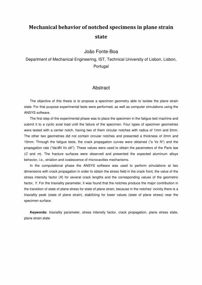
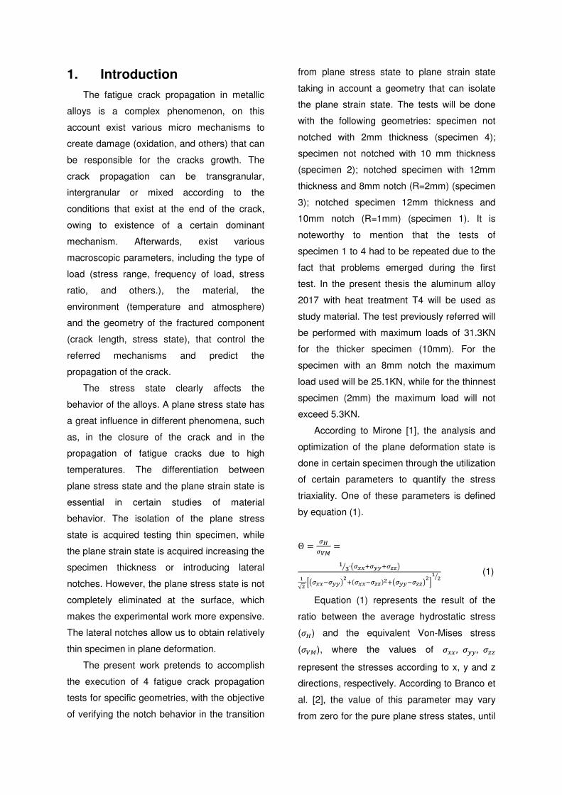
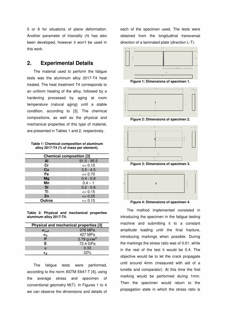
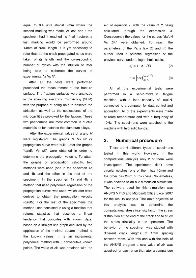
conventional geometry M(T). In Figures 1 to 4

we can observe the dimensions and details of

each of the specimen used. The tests were

obtained from the longitudinal transversal

direction of a laminated plate (direction L-T).

Figure 1: Dimensions of specimen 1.

Figure 2: Dimensions of specimen 2.

Figure 3: Dimensions of specimen 3.

Figure 4: Dimensions of specimen 4.

The method implemented consisted in

introducing the specimen in the fatigue testing

machine and submitting it to a constant

amplitude loading until the final fracture,

introducing markings when possible. During

the markings the stress ratio was of 0.01, while

in the rest of the test it would be 0.4. The

objective would be to let the crack propagate

until around 4mm (measured with aid of a

lunette and comparator). At this time the first

marking would be performed during 1mm.

Then the specimen would return to the

propagation state in which the stress ratio is

equal to 0.4 until almost 9mm where the

second marking was made. At last, and if the

specimen hadn’t reached its final fracture, a

last marking would be performed around

14mm of crack length. It is yet necessary to

refer that, as the crack propagated notes were

taken of its length and the corresponding

number of cycles with the intuition of later

being able to elaborate the curves of

experimental "a Vs N".

After all the tests were performed

proceeded the measurement of the fracture

surface. The fracture surfaces were analyzed

in the scanning electronic microscopy (SEM)

with the purpose of being able to observe the

striaction, as well as the coalescence of the

microcavitities provoked by the fatigue. These

two phenomena are most common in ductile

materials as for instance the aluminum alloys.

After the experimental values of a and N

were registered. The graphs "a Vs N" or

propagation curve were built. Later the graphs

"da/dN Vs ΔK" were obtained in order to

determine the propagation velocity. To attain

the graphs of propagation velocity, two

methods were used (one in the specimen 4a

and 4b and the other in the rest of the

specimen). In the specimen 4a and 4b a

method that used polynomial regression of the

propagation curves was used, which later were

derived to obtain the propagation velocity

(da/dN). For the rest of the specimens the

method used consisted in using a function that

returns statistics that describe a linear

tendency that coincides with known data,

based on a straight line graph acquired by the

application of the minimal square method to

the known values. It is an incremental

polynomial method with 5 consecutive known

points. The value of ΔK was obtained with the

aid of equation 2, with the value of Y being

calculated through the expression 3.

Consequently the values for the curves "da/dN

Vs ΔK" were obtained. To reach the

parameters of the Paris law (C and m) the

author used a potential regression of the

previous curve under a logarithmic scale.

+, = - ∙ � ∙ √./ (2)

- = �sec 34567�� 8

(3)

All of the experimental tests were

performed in a servo-hydraulic fatigue

machine, with a load capacity of 100kN,

connected to a computer for data control and

acquisition. All of the experiments were made

at room temperature and with a frequency of

10Hz. The specimens were attached to the

machine with hydraulic bonds.

3. Numerical procedure

There are 4 different types of specimens

tested in this work. However, in the

computational analysis only 2 of them were

investigated. The specimens don’t have

circular notches, one of them has 10mm and

the other has 2mm of thickness. Nonetheless,

it was decided to do a 2 dimension simulation.

The software used for this simulation was

ANSYS V11.0 and Microsoft Office Excel 2007

for the results analysis. The main objective of

this analysis was to determine the

computational stress intensity factor, the stress

distribution at the end of the crack and to study

the stress triaxiality in the specimen. The

behavior of the specimen was studied with

different crack lengths of 1mm spacing

between them. With this and with the help of

the ANSYS program a new value of ΔK was

acquired for each a, so that later a comparison

could be made with experimental values and to

permit the elaboration of the "Y Vs a"

by using expression 3. With the

graphs, an expression could now be developed

to calculate a value of numerical

of polynomial regressions of the curves

mentioned.

Relatively to the construction of the used

mesh, as well as the modeling of the specimen

by means of FEM the author had to take in

consideration various aspects and details

geometry and boundary conditions used refer

to only half of the specimen due to the existing

symmetrical conditions.

Firstly the KEYPOINTS were defined in the

ANSYS program, followed by the division of

specimen in 6 symmetrical disposed

In this work 3 types of mesh were studied

One more less refined and another one more

refined than that which was used for the final

analysis. The study of the mesh was done with

the initial crack length. To find the various

elements that constitute the mesh, the lines

that compose the geometry of the specimen

were divided in smaller lines. To perform the

study of the mesh convergence t

command (mesh energetic error) of ANSYS

was used, and the values of equivalent

Mises stress was obtained, having both

parameters converged to acceptable values

figure 5 we can observe the mesh used in the

critical zone of the problem (fro

crack). In this area of the specimen the mesh

was the most refined possible without causing

harm to the analysis time and quality of the

results. In the rest of the zones the mesh

refinement was less refined

compromising the quality of the results

could be made with experimental values and to

"Y Vs a" graphs

With the "Y Vs a"

expression could now be developed

numerical Y, as a result

of polynomial regressions of the curves

Relatively to the construction of the used

of the specimen

by means of FEM the author had to take in

consideration various aspects and details. The

geometry and boundary conditions used refer

to only half of the specimen due to the existing

were defined in the

followed by the division of

disposed areas.

In this work 3 types of mesh were studied.

and another one more

refined than that which was used for the final

analysis. The study of the mesh was done with

To find the various

elements that constitute the mesh, the lines

that compose the geometry of the specimen

To perform the

study of the mesh convergence the ERNORM

command (mesh energetic error) of ANSYS

equivalent Von-

stress was obtained, having both

parameters converged to acceptable values. In

figure 5 we can observe the mesh used in the

critical zone of the problem (front side of the

In this area of the specimen the mesh

was the most refined possible without causing

harm to the analysis time and quality of the

In the rest of the zones the mesh

less refined without

e results.

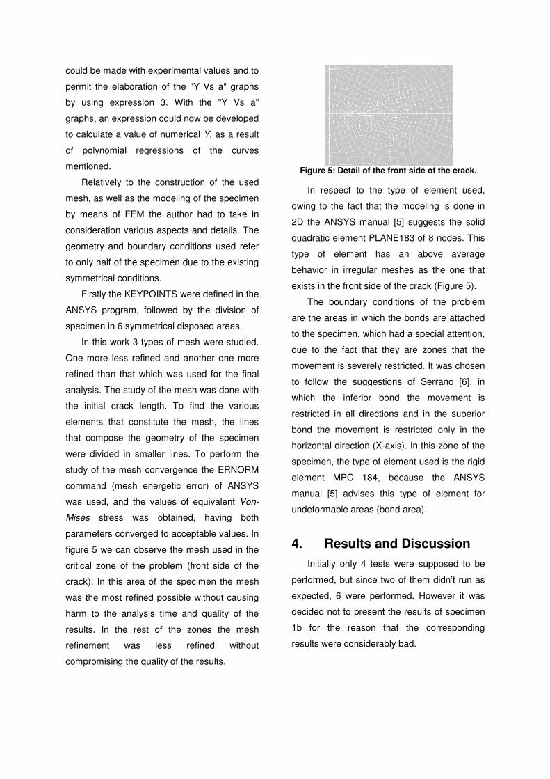
Figure 5: Detail of the front side of the crack

In respect to the type of element used

owing to the fact that the modeling is done in

2D the ANSYS manual [5

quadratic element PLANE183 of 8

type of element has an above average

behavior in irregular meshes as the one that

exists in the front side of the crack (F

The boundary conditions of the problem

are the areas in which the bonds are attached

to the specimen, which had a spec

due to the fact that they are zones that the

movement is severely restricted

to follow the suggestions of

which the inferior bond the movement is

restricted in all directions and in the superior

bond the movement is restricted only in the

horizontal direction (X-axis

specimen, the type of element used is the rigid

element MPC 184, because the

manual [5] advises this type of element for

undeformable areas (bond area

4. Results and

Initially only 4 tests were suppose

performed, but since two of them didn’t run as

expected, 6 were performed. However it was

decided not to present the results of specimen

1b for the reason that the corresponding

results were considerably

Detail of the front side of the crack.

In respect to the type of element used,

owing to the fact that the modeling is done in

[5] suggests the solid

PLANE183 of 8 nodes. This

type of element has an above average

behavior in irregular meshes as the one that

exists in the front side of the crack (Figure 5).

The boundary conditions of the problem

are the areas in which the bonds are attached

, which had a special attention,

due to the fact that they are zones that the

movement is severely restricted. It was chosen

to follow the suggestions of Serrano [6], in

which the inferior bond the movement is

restricted in all directions and in the superior

nt is restricted only in the

axis). In this zone of the

specimen, the type of element used is the rigid

because the ANSYS

dvises this type of element for

bond area).

Results and Discussion

were supposed to be

performed, but since two of them didn’t run as

expected, 6 were performed. However it was

decided not to present the results of specimen

1b for the reason that the corresponding

y bad.

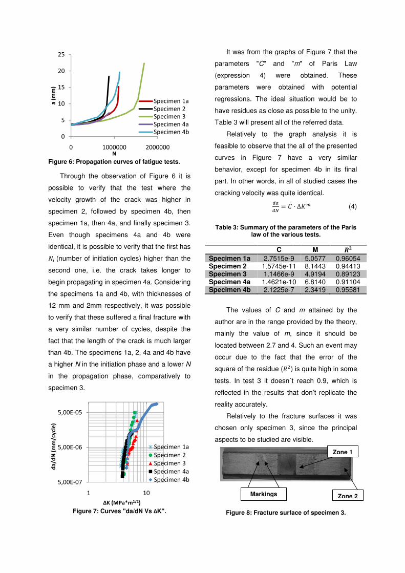
Figure 6: Propagation curves of fatigue

Through the observation of Figure 6 it is

possible to verify that the test where the

velocity growth of the crack was higher in

specimen 2, followed by specimen 4b, then

specimen 1a, then 4a, and finally specimen 3

Even though specimens 4a and 4b were

identical, it is possible to verify that the first has

9: (number of initiation cycles) higher

second one, i.e. the crack takes longer to

begin propagating in specimen 4a

the specimens 1a and 4b, with thicknesses of

12 mm and 2mm respectively, it was possible

to verify that these suffered a final fracture with

a very similar number of cycles

fact that the length of the crack

than 4b. The specimens 1a, 2, 4a and

a higher N in the initiation phase and a

in the propagation phase, comparatively to

specimen 3.

Figure 7: Curves "da/dN Vs

0

5

10

15

20

25

0 1000000 2000000

a (

mm

)

N

5,00E-07

5,00E-06

5,00E-05

1 10

da

/dN

(m

m/c

ycl

e)

ΔK (MPa*m1/2)

fatigue tests.

Through the observation of Figure 6 it is

possible to verify that the test where the

velocity growth of the crack was higher in

specimen 2, followed by specimen 4b, then

a, then 4a, and finally specimen 3.

Even though specimens 4a and 4b were

identical, it is possible to verify that the first has

higher than the

i.e. the crack takes longer to

begin propagating in specimen 4a. Considering

with thicknesses of

it was possible

to verify that these suffered a final fracture with

a very similar number of cycles, despite the

is much larger

1a, 2, 4a and 4b have

in the initiation phase and a lower N

comparatively to

/dN Vs ΔK".

It was from the graphs of Figure 7 that the

parameters "C" and "

(expression 4) were obtained

parameters were obtained with potential

regressions. The ideal situation would be to

have residues as close as possible to the

Table 3 will present all of the referred data

Relatively to the graph analysis it is

feasible to observe that the

curves in Figure 7 have a very

behavior, except for specimen

part. In other words, in all of studied case

cracking velocity was quite identical

;5;< = =

Table 3: Summary of the parameters of the Paris law of the various tests

C

Specimen 1a 2.7515e-9Specimen 2 1.5745e-11Specimen 3 1.1466e-9Specimen 4a 1.4621e-10Specimen 4b 2.1225e-7

The values of C and

author are in the range provided by the theory,

mainly the value of m,

located between 2.7 and 4.

occur due to the fact that the error of the

square of the residue (>8) tests. In test 3 it doesn´t reach

reflected in the results that don’t

reality accurately.

Relatively to the fracture surfaces

chosen only specimen 3,

aspects to be studied are visible

Figure 8: Fracture surface of specimen 3

2000000

Specimen 1a

Specimen 2

Specimen 3

Specimen 4a

Specimen 4b

10

Specimen 1a

Specimen 2

Specimen 3

Specimen 4a

Specimen 4b

Markings

It was from the graphs of Figure 7 that the

"m" of Paris Law

were obtained. These

parameters were obtained with potential

The ideal situation would be to

have residues as close as possible to the unity.

will present all of the referred data.

Relatively to the graph analysis it is

feasible to observe that the all of the presented

curves in Figure 7 have a very similar

except for specimen 4b in its final

l of studied cases the

velocity was quite identical.

∙ ∆+@ (4)

Summary of the parameters of the Paris law of the various tests.

M &A

9 5.0577 0.96054 11 8.1443 0.94413 9 4.9194 0.89123 10 6.8140 0.91104 7 2.3419 0.95581

and m attained by the

author are in the range provided by the theory,

, since it should be

4. Such an event may

occur due to the fact that the error of the

) is quite high in some

test 3 it doesn´t reach 0.9, which is

reflected in the results that don’t replicate the

fracture surfaces it was

3, since the principal

aspects to be studied are visible.

: Fracture surface of specimen 3.

Zone 1

Zone 2

The fracture surfaces are representative of

the different types of fractures due to fatigue

and in them it is possible to identify two distinct

regions, as well as the markings, labeled in

Figure 8.

There are 2 identified zones in the fracture

surfaces. Zone 1 is a smooth region with a

silky and bright aspect, caused by the contact

of the crack surfaces during the propagation

phase [7]. The second region identified by the

fracture surfaces have a more irregular aspect

than the first, much less bright, presenting

various irregularities. In this zone occurs the

final fracture of the specimen when the

transversal section (not cracked) it is not able

to support the applied stress.

. On behalf of the thicker specimens, such

as specimen 3, the propagation line tends to

be curved and this fact is accentuated as we

head towards the interior of the specimen. This

happens due to, in the case of the thinner

specimens, the probable plane stress state of

the specimen due to the fact that it has only

2mm of thickness. In the case of the thicker

specimens the propagation lines tend to curve

as it advances to the interior of the specimen,

owing to the fact that the specimen is close to

the plane strain state. Close to the surface of

the specimen the fact that the lines don´t have

an accentuated curvature is due to the plane

stress state that occurs at the surface of the

specimen.

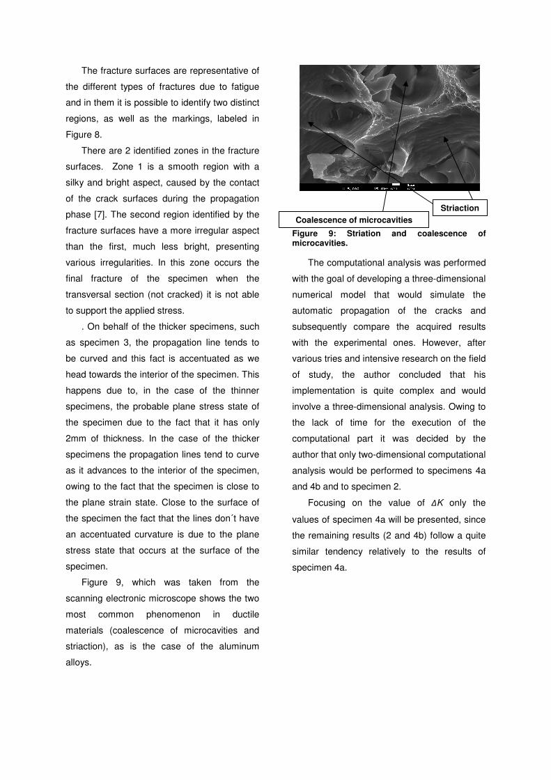
Figure 9, which was taken from the

scanning electronic microscope shows the two

most common phenomenon in ductile

materials (coalescence of microcavities and

striaction), as is the case of the aluminum

alloys.

Figure 9: Striation and coalescence of microcavities.

The computational analysis was performed

with the goal of developing a three-dimensional

numerical model that would simulate the

automatic propagation of the cracks and

subsequently compare the acquired results

with the experimental ones. However, after

various tries and intensive research on the field

of study, the author concluded that his

implementation is quite complex and would

involve a three-dimensional analysis. Owing to

the lack of time for the execution of the

computational part it was decided by the

author that only two-dimensional computational

analysis would be performed to specimens 4a

and 4b and to specimen 2.

Focusing on the value of ΔK only the

values of specimen 4a will be presented, since

the remaining results (2 and 4b) follow a quite

similar tendency relatively to the results of

specimen 4a.

Coalescence of microcavities

Striaction

Figure 10: Comparison of curves ΔK Vs a of specimen 4a.

Analyzing the figure 10 it is possible to

verify a certain discrepancy between the

experimental and computational values, more

accentuated as the length of the crack

increases. Such a discrepancy has an

associated error of 44.5% at the beginning and

44.3% at the end. The error of this specimen

between the computational and experimental

values is high; however it is the lowest of the

three that were studied. Despite this

discrepancy, it’s possible to verify that the

format of the curves, experimental and

computational, has a similar development.

Figure 11 shows the development of the Y

value with the crack growth for the specimen

4a. Through observation of figure 11 it was

found that the experimental and computational

curves don’t coincide, or even close, with

errors in the magnitude of 50%. This high error

occurs probably due to the fact that the

analysis was done in two dimensions.

However, both curves have a quite identical

behavior, with a decline in the initial part, and

as the crack propagates that decline increases,

which agrees with the theory provided for this

type of analysis. To obtain the graph of the

experimental part expression 4 was used, with

a central crack of length 2a in a finite plate of

width W, according to [7]. The computational

curve was acquired by using expression 3. The

value of ΔK used was obtained from the finite

element program ANSYS, being the rest of the

values the same, either for the experimental

part either for the computational part.

Figure 11: Graph "Y Vs a" of specimen 4a.

Finally a polynomial regression of third

order was elaborated to the computational

curve to obtain an expression for the

geometrical factor of stress intensity (Y). The

regression (expression 5) was attained with a

fairly reduced residue (>8 = 0.9866).

- = �−9,1009 × 10J�/� + �4,1135 × 10��/8 −

16,251 × / + 2,0421 (5)

As seen in Figure 12, an expressive

variation appears of the equivalent stress of

Von-Mises in the notch surroundings, i.e.

approximately around the 3.5mm. However, as

we go along the width of the specimen towards

its exterior it is possible to verify a tendency of

the stress value to the remotely applied load

(63,5MPa in the case of specimen 4a).

Figure 12: Distribution of Von-Mises stresses at the front side of specimen 4a.

In relation to the triaxiality parameter we

can observe the results of Figure 13. As it can

be seen in Figure 13 the triaxiality parameter

increases significantly near the notch root, and

0

5

10

15

3 5 7 9

ΔK

(M

Pa

*m

1/2

)

a (mm)

ΔK Vs a

Experimental

Computational

0

1

2

3

0 0,002 0,004 0,006 0,008

Y

a (m)

Y Vs a

Computational

Experimental

0

1000

2000

3000

4000

0 10 20 30Vo

n-M

ise

s st

ress

(MP

a)

Width of specimen(mm)

Evolution of Von-Mises stress

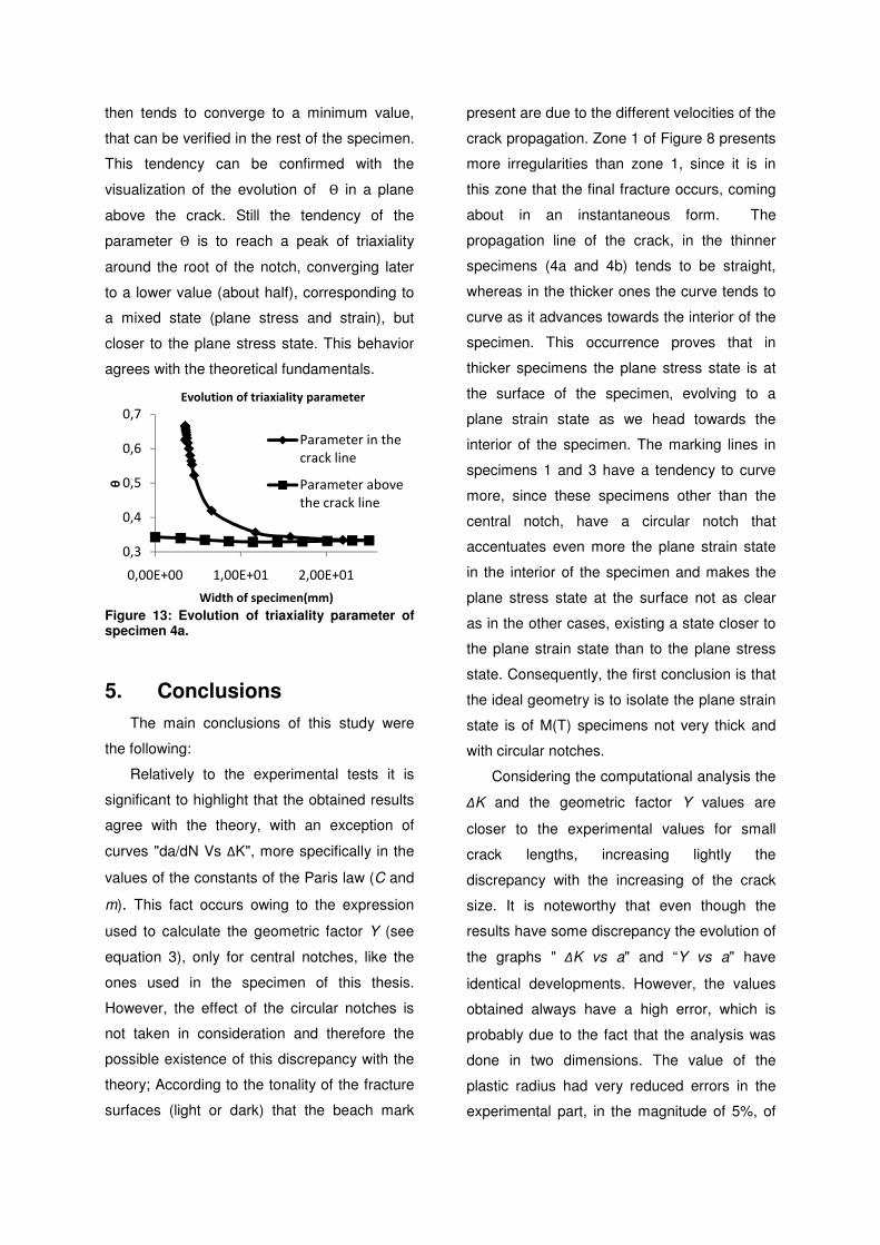
then tends to converge to a minimum value,

that can be verified in the rest of the specimen.

This tendency can be confirmed with the

visualization of the evolution of Θ in a plane

above the crack. Still the tendency of the

parameter Θ is to reach a peak of triaxiality

around the root of the notch, converging later

to a lower value (about half), corresponding to

a mixed state (plane stress and strain), but

closer to the plane stress state. This behavior

agrees with the theoretical fundamentals.

Figure 13: Evolution of triaxiality parameter of specimen 4a.

5. Conclusions

The main conclusions of this study were

the following:

Relatively to the experimental tests it is

significant to highlight that the obtained results

agree with the theory, with an exception of

curves "da/dN Vs ΔK", more specifically in the

values of the constants of the Paris law (C and

m). This fact occurs owing to the expression

used to calculate the geometric factor Y (see

equation 3), only for central notches, like the

ones used in the specimen of this thesis.

However, the effect of the circular notches is

not taken in consideration and therefore the

possible existence of this discrepancy with the

theory; According to the tonality of the fracture

surfaces (light or dark) that the beach mark

present are due to the different velocities of the

crack propagation. Zone 1 of Figure 8 presents

more irregularities than zone 1, since it is in

this zone that the final fracture occurs, coming

about in an instantaneous form. The

propagation line of the crack, in the thinner

specimens (4a and 4b) tends to be straight,

whereas in the thicker ones the curve tends to

curve as it advances towards the interior of the

specimen. This occurrence proves that in

thicker specimens the plane stress state is at

the surface of the specimen, evolving to a

plane strain state as we head towards the

interior of the specimen. The marking lines in

specimens 1 and 3 have a tendency to curve

more, since these specimens other than the

central notch, have a circular notch that

accentuates even more the plane strain state

in the interior of the specimen and makes the

plane stress state at the surface not as clear

as in the other cases, existing a state closer to

the plane strain state than to the plane stress

state. Consequently, the first conclusion is that

the ideal geometry is to isolate the plane strain

state is of M(T) specimens not very thick and

with circular notches.

Considering the computational analysis the

ΔK and the geometric factor Y values are

closer to the experimental values for small

crack lengths, increasing lightly the

discrepancy with the increasing of the crack

size. It is noteworthy that even though the

results have some discrepancy the evolution of

the graphs " ΔK vs a" and “Y vs a" have

identical developments. However, the values

obtained always have a high error, which is

probably due to the fact that the analysis was

done in two dimensions. The value of the

plastic radius had very reduced errors in the

experimental part, in the magnitude of 5%, of

0,3

0,4

0,5

0,6

0,7

0,00E+00 1,00E+01 2,00E+01

θ

Width of specimen(mm)

Evolution of triaxiality parameter

Parameter in the

crack line

Parameter above

the crack line

which in the computational part those errors

were much higher comparatively to the theory.

One of the plausible explanations for this fact

is that the simulations were only done in 2D. In

relation to the triaxiality parameter the results

obtained agree with what was expected, i.e. a

peak of triaxiality was observed at the

surroundings of the notch. This behavior

concurs with what was expected, since the

regions of the specimen away from the zone of

influence of the notch (in terms of Von-Mises

stress field) do not suffer any effect of triaxiality

imposed by this geometrical constrain. This

evolution of the triaxiality parameter confirms

the utility of the notches in the transition from

plane stress state to plane strain state. In a

region close to the notch one may have plane

strain state, of which as one gets away from

the end of the specimen a mixed stated is

verified, but closer to the plane stress state.

The geometries used were, in fact, able to

attain a state close to the plane strain state in

the region of crack propagation, as it was

demanded at the beginning of the dissertation.

The value acquired for the parameter Θ,

despite the fact that it does not approach the

theoretical values (5 or 6), it can already be

considered a plane strain state, since these

values can only be reached in a theoretical

situation, values of this magnitude are rarely

obtained.

References

[1] G. Mirone. Role of stress triaxiality in

elastoplastic characterization and ductile

failure prediction. Engineering Fracture

Mechanics, Vol. 74, pp. 1203-21, 2007.

[2] R. Branco, J. M. Silva, V. Infante, F.

Antunes and F. Ferreira. Using a standard

specimen for crack propagation under

plain strain conditions. International

Journal of Structural Integrity, Vol.1 No.4,

2010.

[3] http://www.matweb.com/

[4] ASTM. Standard terminology relating to

fatigue and fracture testing. ASTM E

1823, 1997.

[5] ANSYS'S Manual ( V-11.0).

[6] B. Serrano. Previsão do tempo de vida de

fadiga da aeronave Epsilon TB-30 da

FAP. Tese de Mestrado. Instituto Superior

Técnico, 2009.

[7] C. A. G. de Moura Branco. Mecânica dos

Materiais. Fundação Calouste

Gulbenkian, 3ª edição, 1998.