Measuring with Timed Patterns

Thomas Ferrere1, Oded Maler1, Dejan Nickovic2, and Dogan Ulus1

1 VERIMAG, CNRS and the University of Grenoble-Alpes, France2 AIT Austrian Institute of Technology GmbH, Vienna, Austria

Abstract. We propose a declarative measurement specification languagefor quantitative performance evaluation of hybrid (discrete-continuous)systems based on simulation traces. We use timed regular expressionswith events to specify patterns that define segments of simulation tracesover which measurements are to be taken. In addition, we associate mea-sure specifications over these patterns to describe a particular type of per-formance evaluation (maximization, average, etc.) to be done over thematched signal segments. The resulting language enables expressive andversatile specification of measurement objectives. We develop an algo-rithm for our measurement framework, implement it in a prototype tool,and apply it in a case study of an automotive communication protocol.Our experiments demonstrate that the proposed technique is usable withvery low overhead to a typical (computationally intensive) simulation.

1 Introduction

Verification consists in checking whether system behaviors, sequences of statesand events, satisfy some specifications. These specifications are expressed in aformalism, for example temporal logic, with well-defined semantics such thatthe satisfaction or violation of a property ϕ by a behavior w can be computedbased on ϕ and w. To perform exhaustive formal verification, property ϕ istypically converted into an automaton A¬ϕ that accepts only violating sequenceswhich is later composed with the system model and checked for emptiness. Suchspecifications are also used in a more lightweight and scalable form of verification(known as runtime verification in software and assertion checking in hardware)where individual behaviors are checked for property satisfaction. In this context,the formal specification language can be used to automatically derive propertymonitors rather than inspect execution traces manually or program monitors byhand. The specification formalism allows us to focus on the observable propertiesof the system we are interested in and write them in a declarative way, separatedfrom their implementation. It is this concept that we export from the qualitativeto the quantitative world.

Properties offer a purely qualitative way to evaluate systems and their be-haviors: correct or incorrect. There are many contexts, however, where we wantalso to associate quantitative measures with systems and their executions. Con-sider for example a real-time system with both safety-critical and non-criticalaspects, evaluated according to the temporal distance between pairs of request

and service events. Its safety-critical part will be evaluated according to whethersome distance goes beyond a hard deadline. In contrast, its non-critical part istypically evaluated based on quality-of-service performance measures which arenumerical in nature, such as the average response time or throughput.

Quantitative measures are used heavily in the design of cyber-physical sys-tems involving heterogeneous components of computational and physical na-tures. Such systems exhibit continuous and hybrid behaviors and are often de-signed using modeling languages such as Simulink, Modelica or hardware de-scription languages. These models are analyzed using a combination of numer-ical and discrete-event simulation, producing traces from which performancemeasures are extracted to evaluate design quality. Measures are computed byapplying various operations such as summation/integration, arithmetical opera-tions, max-min, etc. to certain segments of the simulation trace. The boundariesof these segments are defined according to the occurrence of certain events andpatterns in the trace. When the measures are simple they are realized by in-serting additional observer blocks to the system model but when they are morecomplex, they are extracted using manually-written (and error prone) proceduralscripts that perform computations over the traces.

v

t

t

t

v1

v2

b1

b2

r s t1 t2

Fig. 1. Stopping distance measurement for anti-lock brake systems.

We illustrate how measurements can be used to compare two correct im-plementations of an anti-lock brake system (ABS), which prevents wheels fromlocking during heavy braking or on slippery roads. Figure 1 depicts braking con-trol signals b1 and b2 and velocity signals v1 and v2 for two controller models C1

and C2. The driver starts to brake fully at t = r and then the ABS takes controlat t = s and applies rapid pulsation to prevent locking. Both controllers C1

and C2 satisfy the anti-lock property but we also want to compare the distancecovered during their respective breaking periods. These periods are identified asthose where signal b matches some braking pattern, and are the intervals (r, t1)for C1 and (r, t2) for C2. Integrating vi over respective intervals (r, ti) for i = 1..2we get a numerical measure and conclude that C1 performs better.

In this paper we propose a declarative and formal measure specification lan-guage for automatically extracting measures from hybrid discrete-continuoustraces. The patterns that define the scope of measurements are expressed usinga variant of the timed regular expressions (tre) of [3, 2], specially adapted forthis purpose by adding preconditions, postconditions and events. An additionallanguage layer is used to define the particular measures applied to the matchingsegments. The actual extraction of the measures takes advantage of the recentpattern matching procedure introduced in [19] for computing the set of segmentsof a Boolean signal that match a timed regular expression. In the general case,the number of such matches can be uncountable and the procedure of [19] repre-sents them as a finite union of zones. In our language, where pattern boundariesare punctual events, we obtain a finite number of matches.

The resulting framework provides a step toward making the common prac-tice of quantitative measurement extraction more rigorous, bridging the gapbetween qualitative verification and quantitative performance evaluation. Wedemonstrate the applicability of our approach using the Distributed System In-terface (DSI3) standard protocol [15] developed by the automotive industry. Weformalize in our language measurements of some features described in the stan-dard, extract them from simulation traces and report the performance of ourprototype implementation.

Related Work

The approach proposed in this paper builds upon the timed regular expressionsintroduced in [3, 2] and shown there to be equivalent in expressive power to timedautomata. We omit the renaming operator used for this expressivity theoreticalresult and enrich the formalism with other features that lead to a pattern lan-guage dedicated to measurements, which we call conditional tre. Preconditionand postcondition constraints allow us to express zero-duration events such asrising and falling edges of dense-time Boolean signals. Focusing on patterns thatstart and end with an event, the pattern matching algorithm of [19] returns afinite number of matching segments.

Our approach differs in several respects from monitoring procedures basedon real-time temporal logics and their extensions to real-valued signals such asSTL [16]. In a nutshell here is the difference between satisfaction in temporallogic and matching in regular expression. For any temporal logic with futureoperators, satisfaction of ϕ by a behavior w is defined as (w, 0) |= ϕ. To computethis satisfaction value of ϕ at 0 we need to compute (w, t) |= ψ for some sub-formulas ψ of ϕ and some time t ≥ 0, in other words determine whether somesuffix of w satisfies ψ. This can be achieved by associating with every formula ϕa satisfaction signal relative to w which is true for every t such that (w, t) |= ϕ.On the other hand, the matching of a regular expression ϕ in w is not definedrelative to a single time point but to a pair of points (t, t′) such that the segmentof w between t and t′ satisfies the expression. This property of regular expressionsmakes them ideal for defining intervals that match patterns.

The recent work on assertion-based features [7] is similar in spirit to ours.The authors propose an approach for quantitative evaluation of mixed-signaldesign properties expressed as regular expressions. In contrast to our work, theregular expressions are extended with local variables, which are used to explicitlystore values of interest, such as the beginning and the end time of a matchedpattern. This work addresses the problem of measuring properties (features) ofhybrid automata models using formal methods. We also mention the extensionto tre proposed in [13] that combines specification of real-time events and statesoccurring in continuous-time signals. Their syntax and primitive constructs areinspired by and extend industrial standards PSL [10] and SVA [20]. This workfocuses on a translation from tre to timed automata acceptors, but does notaddress the problem of pattern matching an expression on a concrete trace.

In the context of modeling resource-constrained computations, quantitativelanguages [6] were studied as generalizations of formal languages in which tracesare associated with a real number rather than a Boolean value. The authors useweighted automata to define several classes of quantitative languages and de-termine the trace values by computing maximum, limsup, liminf, limit averageand discounted sum over a (possibly infinite) trace. The ideas of quantitativelanguages are further extended in [14], by defining the model measuring prob-lem. The model checking problems of TCTL and LTL are extended in [21, 11, 1]to a model measuring paradigm by parameterizing the bounds of the temporaloperators. The authors propose algorithms for identifying minimum and max-imum parameter values for which the model satisfies the temporal formula. Asimilar extension is proposed in [4] for signal temporal logic (STL), where boththe temporal bounds and real-valued thresholds are written as parameters andinferred from signals. Robust interpretation of temporal logic specifications [12,9, 8] is another way to associate numbers with traces according to how stronglythey satisfy or violate a property.

Hardware designers and others who use block diagrams for control and signalprocessing often realize measurement using additional observer blocks, but theseare restricted to online measurements. As a result commercial circuit simulationsuites offer scripting languages or built-in functions dedicated to measurementextraction, such as the .measure (Synopsys) and .extract (Mentor Graphics)libraries. The former is structured according to the notion of trigger and tar-get events, the measurement being performed on the segment(s) of the tracein between. This is particularly suited for timing analysis such as rise-time orpropagation time. The latter is more general but relies mostly on functional com-position. Absolute time of events in the trace can be found by threshold crossingfunctions, and then passed on as parameters to other measurement primitives toapply an aggregating function over suitable time intervals. In the approach wepropose, one gains the expressiveness of the language of timed regular expres-sion, that allow to detect complex sequences of events and states in the trace.This facilitates repeated measurements over a sequence of specified patterns, byclearly separating the behavior description from the measure itself.

2 Timed Regular Expression Patterns

In this section, we first recall the definition of the timed regular expressions (tre)from [19]. Such expressions were defined over Boolean signals and in order to usethem for real-valued signals we add predicates on real values to derive Booleansignals. This straightforward extension is still not entirely suitable for definingmeasurement segments, for the simple reason that an arbitrary regular expres-sion may have infinitely many matches. For example an atomic proposition p ismatched by all sub-segments of a dense-time Boolean signal where p continu-ously holds. Consequently in the second part of this section, we propose a novelextension that we call conditional timed regular expressions (ctre). This exten-sion enables to condition the match of a tre to a prefix and suffix, and allowsdefining events of zero duration. We define a restriction to ctre, that we callevent-bounded timed regular expressions (e-tre), which guarantees that the setof patterns matching a e-tre is always finite. Thanks to this finiteness prop-erty, we will use e-tre as the main building block in defining our measurementspecification language.

2.1 Timed Regular Expressions

Let X and B be sets of real and propositional variables and w : [0, d]→ Rm×Bn,wherem = |X| and n = |B|, a multi-dimensional signal of length d. For a variablev ∈ X ∪B we denote by πv(w) the projection of w on its component v.A propositional variable b ∈ B admits a negation ¬b, which value at time t isthe opposite of that of b. For θ a concrete predicate R → B we may create apropositional symbol θ(x) which interpretation at time t will be given by theevaluation of θ on the value of real variable x at time t. We define the projectionof w on ¬b by letting π¬b(w)[t] = 1 − πb(w)[t], and the projection of w onθ(x) by letting πθ(x)(w)[t] = θ(πx(w)[t]). A proposition p is taken to be either avariable b ∈ B, a predicate θ(x) over some real variable x, or their negation ¬band ¬θ(x) respectively. We assume a given set of real predicates and take P theset of propositions derived from real and propositional variables as described. Asignal is said to have finite variability if for every proposition p ∈ P the set ofdiscontinuities of πp(w) is finite.

We now define the syntax of timed regular expressions according to the fol-lowing grammar:

ϕ := ε | p | ϕ1 · ϕ2 | ϕ1 ∪ ϕ2 | ϕ1 ∩ ϕ2 | ϕ∗ | 〈ϕ〉I

where p is a proposition of P , and I is an interval of R+.

The semantics of a timed regular expression ϕ with respect to a signal wand times t ≤ t′ in [0, d] is given in terms of a satisfaction relation (w, t, t′) |= ϕ

inductively defined as follows:

(w, t, t′) |= ε ↔ t = t′

(w, t, t′) |= p ↔ t < t′ and ∀ t < t′′ < t′, πp(w)[t′′] = 1(w, t, t′) |= ϕ1 · ϕ2 ↔ ∃ t ≤ t′′ ≤ t′, (w, t, t′′) |= ϕ1 and (w, t′′, t′) |= ϕ2

(w, t, t′) |= ϕ1 ∪ ϕ2 ↔ (w, t, t′) |= ϕ1 or (w, t, t′) |= ϕ2

(w, t, t′) |= ϕ1 ∩ ϕ2 ↔ (w, t, t′) |= ϕ1 and (w, t, t′) |= ϕ2

(w, t, t′) |= ϕ∗ ↔ (w, t, t′) |= ε or (w, t, t′) |= ϕ · ϕ∗(w, t, t′) |= 〈ϕ〉I ↔ t′ − t ∈ I and (w, t, t′) |= ϕ

Following the definitions in [19], we characterize the set of segments of wthat match an expression ϕ by their match set. The match set of expression ϕover w is the set of all pairs (t, t′) such that the segment of w between t and t′

matches ϕ.

Definition 1 (Match Set). For any signal w and expression ϕ, we define theirmatch set as

M(ϕ,w) := (t, t′) ∈ R2 | (w, t, t′) |= ϕ

We recall that a match set is a subset of [0, d] × [0, d] confined to the uppertriangle defined by t ≤ t′ taking t, t′ the first and second coordinates of R2.It has been established that such a set can always be represented as a finiteunion of zones. In Rn, zones are a special class of convex polytopes definable byintersections of inequalities of the form xi ≥ ai, xi ≤ bi and xi − xj ≤ ci,j orcorresponding strict inequalities. We say that a zone is punctual when the valueof each variable is uniquely defined, with for instance ai = bi for all i = 1..n. Weuse zones in R2 to describe the relation between t and t′ in a match set.

Theorem 1 ([19]). For any finite variability signal w and tre ϕ, the setM(ϕ,w) is a finite union of zones.

2.2 Conditional TRE

We propose in the sequel conditional timed regular expressions (ctre) that ex-tend tre. This extension enables to condition the match of a tre to a prefixor a suffix. We introduce in the syntax of ctre two new binary operators, “?”for preconditions, and “!” for postconditions. For some expressions ϕ1 and ϕ2

a trace w matches the expression ϕ1 ?ϕ2 at (t, t′) if it matches ϕ2 and thereis an interval ending at t where w matches ϕ1. Symmetrically w matches theexpression ϕ1 !ϕ2 at (t, t′) if it matches ϕ1 and there is an interval beginning att′ where w matches ϕ2. We define formally the semantics of these operators forϕ1, ϕ2 arbitrary ctre and w an arbitrary signal as follows:

(w, t, t′) |= ϕ1 ?ϕ2 ↔ (w, t, t′) |= ϕ2 and ∃t′′ ≤ t, (w, t′′, t) |= ϕ1

(w, t, t′) |= ϕ1 !ϕ2 ↔ (w, t, t′) |= ϕ1 and ∃t′′ ≥ t′, (w, t′, t′′) |= ϕ2

A precondition ϕ1 and a postcondition ϕ3 can be associated to an expression ϕ2

independently as we have ϕ1 ?(ϕ2 !ϕ3) ≡ (ϕ1 ?ϕ2) !ϕ3 so that such expressions

may be noted ϕ1 ?ϕ2 !ϕ3 without ambiguity. Associating several conditions canform a sequential condition as with (ϕ1 ?ϕ2) ?ϕ3 ≡ (ϕ1 · ϕ2) ?ϕ3, or conjointconditions as with ϕ1 ?(ϕ2 ?ϕ3) ≡ (ϕ1 ?ϕ3) ∩ (ϕ2 ?ϕ3). There are further rela-tionships with respect to other tre operators, which we will not detail.

2.3 TRE with Events

Another important aspect of ctre is that they enable defining rise and fallevents of zero duration associated to propositional terms. The rise edge ↑ p associ-ated to the propositional term p is obtained by syntactic sugar as ↑ p := ¬p ? ε ! p,while the fall edge ↓ p corresponds to ↓ p := ↑¬p. We now define a restriction ofctre that we call tre with events. This sub-class of ctre consists of restrictingthe use of conditional operators to the definition of events. The introduction ofevents in tre still guarantees the finite representation of their match set.

Corollary 1 (of Theorem 1). For any finite variability signal w and tre withevents ϕ, the set M(ϕ,w) is a finite union of zones.

Proof. By induction on the expression structure. For expressions of the formϕ = ↑ p, the match set M(ϕ,w) is of the form (t, t) : t ∈ R. By finitevariability hypothesis R is finite as contained in the set of discontinuities of p,and in particularM(ϕ,w) is a finite union of punctual zones. All other operatorsare part of the grammar of timed regular expressions, and the proof of Theorem 1grants us the property.

In what follows we consider events to be part of the syntax of timed regularexpressions, and will just write tre instead of tre with events.

Remark Our support for events is minimal as compared to the real-time regu-lar expressions of [13] where the authors use special operators ##0 and ##1 forevent concatenation. Their work extends discrete-time specification languages,which have the supplementary notion of clocks noted @(↑ c) with c a Booleanvariable, and the implicit notion of clock context. A clock @(↑ c) can then beused in conjunction with a proposition p to form a clocked event noted @(↑ c) p.Such an event allows to probe the value of p at the exact times where ↑ c occurs,which we did not consider. Assuming we dispose of atomic expressions @(↑ c) pholding punctually at times such that ↑ c occurs and p is true, the event con-catenation ##1 can be emulated by @(↑ c) p ##1 @(↑ d) q ≡ @(↑ c) p·d∗ ·¬d · @(↑ d) q.

We now say that a tre is event-bounded when of the form ↑ p, ψ1 · ϕ · ψ2,ψ1 ∪ ψ2, or ψ1 ∩ ϕ with p a proposition, and ψ1, ψ2 event-bounded tre. Suchexpressions, that we call e-tre for short, have an important “well-behaving”property as follows. Given an arbitrary finitely variable signal w, an e-tre canbe matched in w only a finite number of times. In the following lemma, wedemonstrate that the match set for arbitrary finite signal w and e-tre ψ consistsof a finite number of points (t, t′) with t an occurrence of a begin event and t′

an occurrence of an end event.

Lemma 1. Given an e-tre ψ and a signal w, their associated match setM(ψ,w)is finite.

Proof. By induction on the expression structure. Consider an arbitrary signal wand an event ↑ p; by finite variability assumption there are finitely many timepoints in w where ↑ p occurs, so that its match set relatively to w is finite. Nowlet ψ be an e-tre of the form ψ = ψ1 · ϕ · ψ2. The signal w matches ψ on thesegment (t, t′) if and only if there exists some times s and s′ such that w matchesψ1 on (t, s) and matches ψ2 on (s′, t′). By induction hypothesis there are finitelymany such times t, t′, s and s′ so that ψ itself has a finite number of matches.One can easily see that the finiteness of the match set is also preserved by unionsand intersections ψ1 ∪ ψ2 and ψ1 ∩ ϕ, which concludes our proof.

3 Measuring with Conditional TRE

In this section, we propose a language for describing mixed-signal measures, anda procedure to compute such measures. In our approach, we will use measurepatterns based on timed regular expressions to specify signal segments of interest.More precisely, a measure pattern consists of three parts: (1) the main pattern;(2) the precondition; and (3) the postcondition. The main pattern is an e-trethat specifies the portion of the signal over which the measure is taken. Usinge-tre to express main patterns ensures the finiteness of signal segments, whilepre- and post- conditions expressed as general tre allow to define additionalconstraints. We formally define measure patterns as follows.

Definition 2 (Measure Pattern). A measure pattern ϕ is a ctre of the formα ?ψ !β, where α and β are tre, while ψ is an e-tre

Note that preconditions and postconditions can be made optional by using ε aswe have ε ?ϕ ≡ ϕ and ϕ ! ε ≡ ϕ. In what follows we may use simpler formulas toexpress their semantic equivalent, for instance writing ϕ to refer to the measurepattern ε ?ϕ ! ε.

According to previous definitions, the match set of a measure pattern α ?ψ !βgives us the set of all segments of the signal, represented as couples (t, t′), suchthat (w, t, t′) |= ψ, and w satisfies both the precondition α before t and thepostcondition β after t′.

Proposition 1. For any signal w and a pattern ϕ = α ?ψ !β, their associatedmatch set set is given by

M(ϕ,w) = (t, t′) : ∃s ≤ t ≤ t′ ≤ s′, (w, s, t) |= αand (w, t, t′) |= ψand (w, t′, s′) |= β

Theorem 2 (Match set Finiteness). For any signal w and measure patternϕ = α ?ψ !β, their associated match set M(ϕ,w) is finite.

Proof. This is a direct consequence of Lemma 1. The setM(ϕ,w) is included inM(ψ,w), which makes it finite.

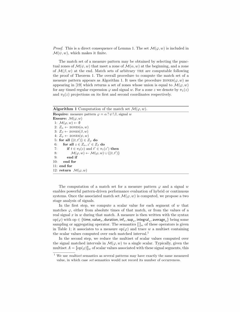
The match set of a measure pattern may be obtained by selecting the punc-tual zones ofM(ψ,w) that meet a zone ofM(α,w) at the beginning, and a zoneof M(β,w) at the end. Match sets of arbitrary tre are computable followingthe proof of Theorem 1. The overall procedure to compute the match set of ameasure pattern appears as Algorithm 1. It uses the procedure zones(ϕ,w) asappearing in [19] which returns a set of zones whose union is equal to M(ϕ,w)for any timed regular expression ϕ and signal w. For a zone z we denote by π1(z)and π2(z) projections on its first and second coordinates respectively.

Algorithm 1 Computation of the match set M(ϕ,w).

Require: measure pattern ϕ = α ?ψ !β, signal wEnsure: M(ϕ,w)1: M(ϕ,w)← ∅2: Zα ← zones(α,w)3: Zβ ← zones(β,w)4: Zψ ← zones(ψ,w)5: for all (t, t′) ∈ Zψ do6: for all z ∈ Zα, z′ ∈ Zβ do7: if t ∈ π2(z) and t′ ∈ π1(z′) then8: M(ϕ,w)←M(ϕ,w) ∪ (t, t′)9: end if

10: end for11: end for12: return M(ϕ,w)

The computation of a match set for a measure pattern ϕ and a signal wenables powerful pattern-driven performance evaluation of hybrid or continuoussystems. Once the associated match setM(ϕ,w) is computed, we propose a twostage analysis of signals.

In the first step, we compute a scalar value for each segment of w thatmatches ϕ, either from absolute times of that match, or from the values of areal signal x in w during that match. A measure is then written with the syntaxop(ϕ) with op ∈ time, valuex, duration, infx, supx, integralx, averagex being somesampling or aggregating operator. The semantics [[ ]]w of these operators is givenin Table 1; it associates to a measure op(ϕ) and trace w a multiset containingthe scalar values computed over each matched interval.1

In the second step, we reduce the multiset of scalar values computed overthe signal matched intervals in M(ϕ,w) to a single scalar. Typically, given themultiset A = [[op(ϕ)]]w of scalar values associated with these signal segments, this

1 We use multiset semantics as several patterns may have exactly the same measuredvalue, in which case set semantics would not record its number of occurrences.

Table 1. Standard measure operators.

[[time(↑ p)]]w = t : (t, t) ∈M(↑ p, w)[[valuex(↑ p)]]w = πx(w)[t] : (t, t) ∈M(↑ p, w)[[duration(ϕ)]]w = t′ − t : (t, t′) ∈M(ϕ,w)[[infx(ϕ)]]w = mint≤τ≤t′ πx(w)(τ) : (t, t′) ∈M(ϕ,w)[[supx(ϕ)]]w = maxt≤τ≤t′ πx(w)(τ) : (t, t′) ∈M(ϕ,w)[[integralx(ϕ)]]w =

∫ t′tπx(w)(τ)dτ : (t, t′) ∈M(ϕ,w)

[[averagex(ϕ)]]w = 1t′−t

∫ t′tπx(w)(τ)dτ : (t, t′) ∈M(ϕ,w)

phase consists in computing standard statistical indicators over A, such as theaverage, maximum, minimum or standard deviation. This final step is optional,the set of basic measurements sometimes provides sufficient information.

Anti-lock Brake System Example We now refer back to our first examplefrom Figure 1 and propose measure pattern formalization to evaluate perfor-mance of the controller. We first formalize the pattern of a brake control signalb under a (heavy) braking situation. The main pattern ψ starts with a rise eventon b and a braking period with the duration in I, continues with one or morepulses with duration in J , and ends with a fall event on b:

ψ := ↑ b · 〈b〉I · 〈¬b · b〉+J · ↓ b

We also need to ensure that the speed should be zero at the end of brakingsituation, with the postcondition β := (v ≤ 0). Finally, we can measure thestopping distance using the expression

integralv(ψ !β)

integrating v over intervals matching the measure pattern.

4 Case Study

4.1 Distributed Systems Interface

Distributed systems interface (DSI3) is a flexible and powerful bus standard [15]developed by the automotive industry. It is designed to interconnect multipleremote sensor and actuator devices to a controller. The controller interacts withthe sensor devices via so-called voltage and current lines. In this paper we focuson two phases of the DSI3 protocol:

– the initialization phase called the discovery mode;

– one of the stationary phases called the command and response mode.

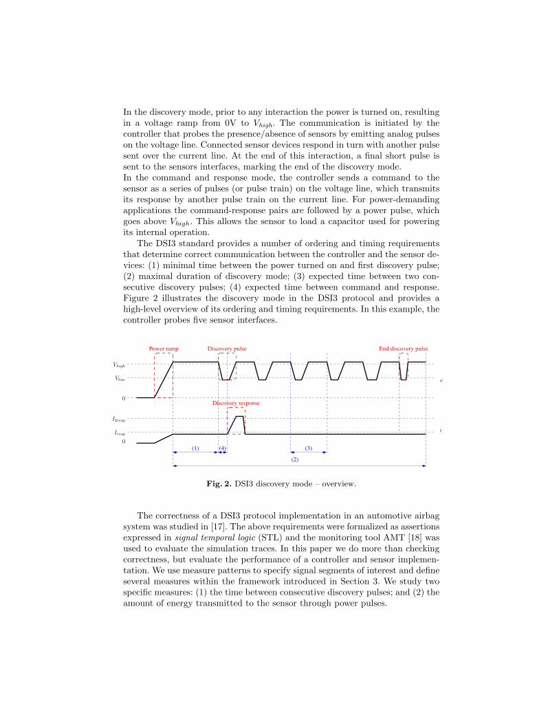
In the discovery mode, prior to any interaction the power is turned on, resultingin a voltage ramp from 0V to Vhigh. The communication is initiated by thecontroller that probes the presence/absence of sensors by emitting analog pulseson the voltage line. Connected sensor devices respond in turn with another pulsesent over the current line. At the end of this interaction, a final short pulse issent to the sensors interfaces, marking the end of the discovery mode.In the command and response mode, the controller sends a command to thesensor as a series of pulses (or pulse train) on the voltage line, which transmitsits response by another pulse train on the current line. For power-demandingapplications the command-response pairs are followed by a power pulse, whichgoes above Vhigh. This allows the sensor to load a capacitor used for poweringits internal operation.

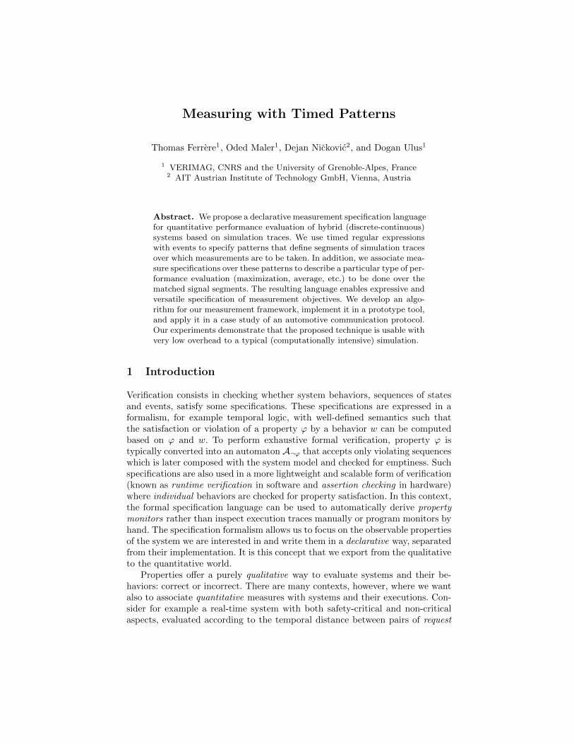
The DSI3 standard provides a number of ordering and timing requirementsthat determine correct communication between the controller and the sensor de-vices: (1) minimal time between the power turned on and first discovery pulse;(2) maximal duration of discovery mode; (3) expected time between two con-secutive discovery pulses; (4) expected time between command and response.Figure 2 illustrates the discovery mode in the DSI3 protocol and provides ahigh-level overview of its ordering and timing requirements. In this example, thecontroller probes five sensor interfaces.

(1) (4) (3)

(2)

Discovery response

Power ramp Discovery pulse End discovery pulse

0

Vlow

Vhigh

0

I2resp

Iresp

v

i

Fig. 2. DSI3 discovery mode – overview.

The correctness of a DSI3 protocol implementation in an automotive airbagsystem was studied in [17]. The above requirements were formalized as assertionsexpressed in signal temporal logic (STL) and the monitoring tool AMT [18] wasused to evaluate the simulation traces. In this paper we do more than checkingcorrectness, but evaluate the performance of a controller and sensor implemen-tation. We use measure patterns to specify signal segments of interest and defineseveral measures within the framework introduced in Section 3. We study twospecific measures: (1) the time between consecutive discovery pulses; and (2) theamount of energy transmitted to the sensor through power pulses.

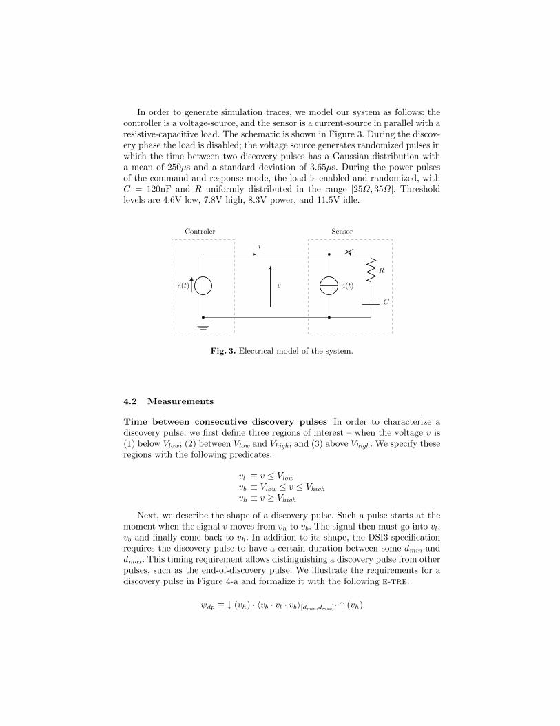
In order to generate simulation traces, we model our system as follows: thecontroller is a voltage-source, and the sensor is a current-source in parallel with aresistive-capacitive load. The schematic is shown in Figure 3. During the discov-ery phase the load is disabled; the voltage source generates randomized pulses inwhich the time between two discovery pulses has a Gaussian distribution witha mean of 250µs and a standard deviation of 3.65µs. During the power pulsesof the command and response mode, the load is enabled and randomized, withC = 120nF and R uniformly distributed in the range [25Ω, 35Ω]. Thresholdlevels are 4.6V low, 7.8V high, 8.3V power, and 11.5V idle.

e(t) a(t)

R

C

Controler Sensor

i

v

Fig. 3. Electrical model of the system.

4.2 Measurements

Time between consecutive discovery pulses In order to characterize adiscovery pulse, we first define three regions of interest – when the voltage v is(1) below Vlow; (2) between Vlow and Vhigh; and (3) above Vhigh. We specify theseregions with the following predicates:

vl ≡ v ≤ Vlowvb ≡ Vlow ≤ v ≤ Vhighvh ≡ v ≥ Vhigh

Next, we describe the shape of a discovery pulse. Such a pulse starts at themoment when the signal v moves from vh to vb. The signal then must go into vl,vb and finally come back to vh. In addition to its shape, the DSI3 specificationrequires the discovery pulse to have a certain duration between some dmin anddmax. This timing requirement allows distinguishing a discovery pulse from otherpulses, such as the end-of-discovery pulse. We illustrate the requirements for adiscovery pulse in Figure 4-a and formalize it with the following e-tre:

ψdp ≡ ↓ (vh) · 〈vb · vl · vb〉[dmin,dmax]· ↑ (vh)

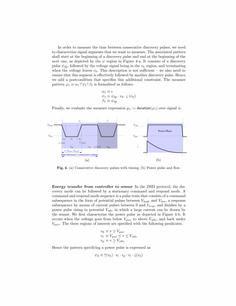
In order to measure the time between consecutive discovery pulses, we needto characterize signal segments that we want to measure. The associated patternshall start at the beginning of a discovery pulse and end at the beginning of thenext one, as depicted by the ψ region in Figure 4-a. It consists of a discoverypulse ψdp, followed by the voltage signal being in the vh region, and terminatingwhen the voltage leaves vh. This description is not sufficient – we also need toensure that this segment is effectively followed by another discovery pulse. Hencewe add a postcondition that specifies this additional constraint. The measurepattern ϕ1 ≡ α1 ?ψ1 !β1 is formalized as follows.

α1 ≡ εψ1 ≡ ψdp · vh· ↓ (vh)β1 ≡ ψdp

Finally, we evaluate the measure expression µ1 := duration(ϕ1) over signal w.

time between 2 consecutive pulses

∈ [dmin, dmax]

ψ β

↓ (vh)

Vlow

Vhigh

vb vbvl

vhrdp rdp

↓ (vh) ↑ (vh)

(a)

Power Phase

i

Vpwr

Vidle

(b)

Fig. 4. (a) Consecutive discovery pulses with timing; (b) Power pulse and flow.

Energy transfer from controller to sensor In the DSI3 protocol, the dis-covery mode can be followed by a stationary command and respond mode. Acommand and respond mode sequence is a pulse train that consists of a commandsubsequence in the form of potential pulses between Vhigh and Vlow, a responsesubsequence by means of current pulses between 0 and Iresp, and finishes by apower pulse rising to potential Vidle in which a large current can be drawn bythe sensor. We first characterize the power pulse as depicted in Figure 4-b. Itoccurs when the voltage goes from below Vpwr to above Vidle, and back underVpwr. The three regions of interest are specified with the following predicates.

vh ≡ v ≥ Vpwr

vt ≡ Vpwr ≤ v ≤ Vidlevp ≡ v ≥ Vidle

Hence the pattern specifying a power pulse is expressed as

ψ2 ≡ ↑(vh) · vt · vp · vt · ↓(vh)

The measure pattern does not have pre- or post-conditions as all other commu-nications occur with v below Vidle, hence α2 = β2 = ε. The measure pattern ϕ2

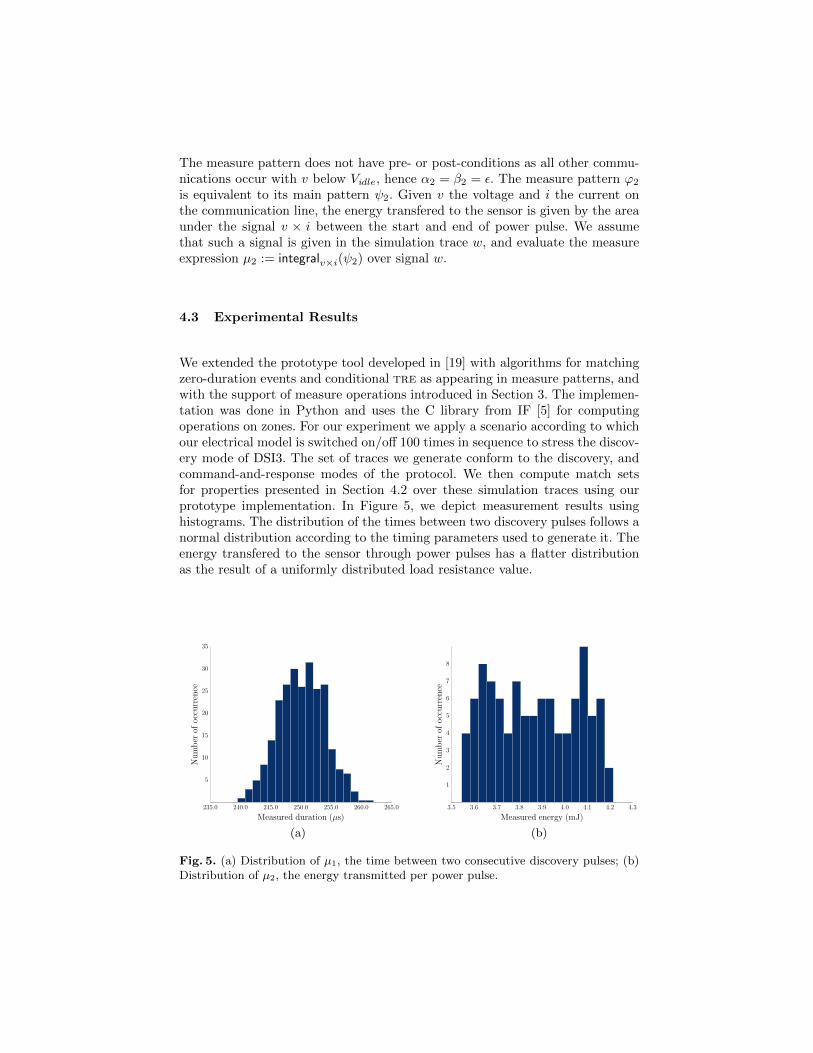
is equivalent to its main pattern ψ2. Given v the voltage and i the current onthe communication line, the energy transfered to the sensor is given by the areaunder the signal v × i between the start and end of power pulse. We assumethat such a signal is given in the simulation trace w, and evaluate the measureexpression µ2 := integralv×i(ψ2) over signal w.

4.3 Experimental Results

We extended the prototype tool developed in [19] with algorithms for matchingzero-duration events and conditional tre as appearing in measure patterns, andwith the support of measure operations introduced in Section 3. The implemen-tation was done in Python and uses the C library from IF [5] for computingoperations on zones. For our experiment we apply a scenario according to whichour electrical model is switched on/off 100 times in sequence to stress the discov-ery mode of DSI3. The set of traces we generate conform to the discovery, andcommand-and-response modes of the protocol. We then compute match setsfor properties presented in Section 4.2 over these simulation traces using ourprototype implementation. In Figure 5, we depict measurement results usinghistograms. The distribution of the times between two discovery pulses follows anormal distribution according to the timing parameters used to generate it. Theenergy transfered to the sensor through power pulses has a flatter distributionas the result of a uniformly distributed load resistance value.

235.0 240.0 245.0 250.0 255.0 260.0 265.0

Measured duration (µs)

5

10

15

20

25

30

35

Nu

mb

erof

occ

urr

ence

3.5 3.6 3.7 3.8 3.9 4.0 4.1 4.2 4.3

Measured energy (mJ)

1

2

3

4

5

6

7

8

Nu

mb

erof

occ

urr

ence

(a) (b)

Fig. 5. (a) Distribution of µ1, the time between two consecutive discovery pulses; (b)Distribution of µ2, the energy transmitted per power pulse.

We then compared the execution times to compute measurements, using aperiodic sampling with different sampling rates – note that our method supportsvariable step sampling without extra cost. The computation times are given inTable 2 with the detailed computation time needed for predicate evaluation (Tp),match set computation (Tm), measure aggregation (Ta) and total computationtime (T ). Computation of match sets does not depend on the number of samplesbut on the number of uniform intervals of atomic propositions; evaluation of realpredicates by linear interpolation, and computing measures like integration canbe done in time linear in the number of samples.

Table 2. Computation times (s)

Measure µ1 Measure µ2

# samples Tp Tm Ta T Tp Tm Ta T

1M 0.047 0.617 0.000 0.664 0.009 0.004 0.011 0.0245M 0.197 0.612 0.000 0.809 0.050 0.005 0.047 0.10310M 0.386 0.606 0.000 0.992 0.101 0.005 0.100 0.21620M 0.759 0.609 0.000 1.368 0.203 0.005 0.260 0.468

5 Conclusion and Future Work

We presented a formal measurement specification language that can be usedfor evaluating cyber-physical systems based on their simulation traces. Startingfrom a declarative specification of the patterns that should be matched in thesegments to be measured, we apply a pattern matching algorithm for timedregular expressions to find out the scope of measurements. The applicability ofour framework was demonstrated on a standard mixed-signal communicationprotocol from the automotive domain.

In the future, we plan to develop an online extension of the presented patternmatching and measurement procedure. It will enable the application of measure-ments during the simulation process as well as performing measurements on realcyber-physical systems during their execution. We believe that the extension ofregular expressions that we introduced is sufficiently expressive to capture com-mon mixed signal properties, and could be used in other application domains,something that we intend to explore further.

Acknowledgements This work was supported by ANR project CADMIDIA,and the MISTRAL project A-1341-RT-GP coordinated by the European DefenceAgency (EDA) and funded by 8 contributing Members (France, Germany, Italy,Poland, Austria, Sweden, Netherlands and Luxembourg) in the framework ofthe Joint Investment Programme on Second Innovative Concepts and EmergingTechnologies (JIP-ICET 2).

References

1. Rajeev Alur, Kousha Etessami, Salvatore La Torre, and Doron Peled. Parametrictemporal logic for ”model measuring”. ACM Transactions on Computational Logic(TOCL), 2(3):388–407, 2001.

2. Eugene Asarin, Paul Caspi, and Oded Maler. A Kleene theorem for timed au-tomata. In Logic in Computer Science (LICS), pages 160–171, 1997.

3. Eugene Asarin, Paul Caspi, and Oded Maler. Timed regular expressions. Journalof ACM, 49(2):172–206, 2002.

4. Eugene Asarin, Alexandre Donze, Oded Maler, and Dejan Nickovic. Parametricidentification of temporal properties. In Runtime Verification (RV), pages 147–160,2011.

5. Marius Bozga, Susanne Graf, and Laurent Mounier. IF-2.0: A validation envi-ronment for component-based real-time systems. In Computer Aided Verifica-tion, 14th International Conference, CAV 2002,Copenhagen, Denmark, July 27-31,2002, Proceedings, pages 343–348, 2002.

6. Krishnendu Chatterjee, Laurent Doyen, and Thomas A. Henzinger. Quantitativelanguages. ACM Transactions on Computational Logic (TOCL), 11(4):23, 2010.

7. Antonio Anastasio Bruto da Costa and Pallab Dasgupta. Formal interpretation ofassertion-based features on AMS designs. IEEE Design & Test, 32(1):9–17, 2015.

8. Alexandre Donze, Thomas Ferrere, and Oded Maler. Efficient robust monitoringfor STL. In Computer Aided Verification (CAV), pages 264–279, 2013.

9. Alexandre Donze and Oded Maler. Robust satisfaction of temporal logic over real-valued signals. In Formal Modeling and Analysis of Timed Systems (FORMATS),pages 92–106, 2010.

10. Cindy Eisner and Dana Fisman. A practical introduction to PSL. Springer, 2006.11. E. Allen Emerson and Richard J. Trefler. Parametric quantitative temporal rea-

soning. In Logic in Computer Science (LICS), pages 336–343, 1999.12. Georgios E. Fainekos and George J. Pappas. Robustness of temporal logic specifi-

cations for continuous-time signals. Theoretical Computer Science, 410(42), 2009.13. John Havlicek and Scott Little. Realtime regular expressions for analog and mixed-

signal assertions. In Formal Methods in Computer-Aided Design (FMCAD), pages155–162, 2011.

14. Thomas A. Henzinger and Jan Otop. From model checking to model measuring.In Conference on Concurrency Theory (CONCUR), pages 273–287, 2013.

15. Distributed System Interface. DSI3 Bus Standard. DSI Consortium.16. Oded Maler and Dejan Nickovic. Monitoring properties of analog and mixed-signal

circuits. STTT, 15(3):247–268, 2013.17. Thang Nguyen and Dejan Nickovic. Assertion-based monitoring in practice - check-

ing correctness of an automotive sensor interface. In Formal Methods for IndustrialCritical Systems (FMICS), pages 16–32, 2014.

18. Dejan Nickovic and Oded Maler. AMT: A property-based monitoring tool foranalog systems. In Formal Modeling and Analysis of Timed Systems (FORMATS),pages 304–319, 2007.

19. Dogan Ulus, Thomas Ferrere, Eugene Asarin, and Oded Maler. Timed patternmatching. In Formal Modeling and Analysis of Timed Systems (FORMATS), pages222–236, 2014.

20. Srikanth Vijayaraghavan and Meyyappan Ramanathan. A practical guide for Sys-temVerilog assertions. Springer, 2006.

21. Farn Wang. Parametric timing analysis for real-time systems. Information andComputation, 130(2):131–150, 1996.