Policy Research Working Paper 8836

Measuring the Unmeasured

Combining Technology and Behavioral Insights to Improve Measurement of Business Outcomes

Stephen J. Anderson Christy Lazicky

Bilal Zia

Development Economics Development Research GroupApril 2019

Pub

lic D

iscl

osur

e A

utho

rized

Pub

lic D

iscl

osur

e A

utho

rized

Pub

lic D

iscl

osur

e A

utho

rized

Pub

lic D

iscl

osur

e A

utho

rized

Produced by the Research Support Team

Abstract

The Policy Research Working Paper Series disseminates the findings of work in progress to encourage the exchange of ideas about development issues. An objective of the series is to get the findings out quickly, even if the presentations are less than fully polished. The papers carry the names of the authors and should be cited accordingly. The findings, interpretations, and conclusions expressed in this paper are entirely those of the authors. They do not necessarily represent the views of the International Bank for Reconstruction and Development/World Bank and its affiliated organizations, or those of the Executive Directors of the World Bank or the governments they represent.

Policy Research Working Paper 8836

Business survey outcomes for micro and small firms are notoriously noisy, with multiple sources of measurement and recall error. This paper introduces a new survey meth-odology that combines automatic consistency checks of electronic data collection with triangulation and dynamic adjustment to arrive at more precise estimates of business performance. The methodology uses insights from behav-ioral science to lower the cognitive cost of initial recall and establishes salient and relevant anchors to allow for dynamic triangulation and adjustment toward a final estimate. The validity of this method is field tested against traditional

performance measures as well as administrative data across three emerging markets: Ghana, Rwanda, and Uganda. The results show significant upward adjustment from traditional measures for both sales and profits, a lower coefficient of variation in the cross-section, and higher autocorrelation in panel data. Comparisons with administrative data further confirm a higher correlation and closer magnitude relative to traditional measures. This research reconciles recom-mendations for increased attention to survey design with a method to leverage electronic survey technology beyond consistency checks.

This paper is a product of the Development Research Group, Development Economics. It is part of a larger effort by the World Bank to provide open access to its research and make a contribution to development policy discussions around the world. Policy Research Working Papers are also posted on the Web at http://www.worldbank.org/prwp. The authors may be contacted at bzia@worldbank.org.

Measuring the Unmeasured:

Combining Technology and Behavioral Insights to Improve Measurement of

Business Outcomes

Stephen J. Anderson

Christy Lazicky

Bilal Zia *

JEL Codes: O12, O16, C81, C93, M41

Keywords: Microenterprises, SMEs, Measurement, Underreporting, Evaluation, Survey Methods

* Anderson: Stanford Graduate School of Business (sjanderson@stanford.edu); Zia: World Bank

(bzia@worldbank.org); Lazicky: IDinsight (christy.lazicky@idinsight.org). We thank the Innovation for Poverty

Action (IPA) country offices in Ghana, Rwanda and Uganda for hosting our study and for excellent data collection

activities. Special thanks to Lukas Autenried for valuable research assistance, as well as Augustine Owusu, Alyson

Caito, and Stephen Kagera for great fieldwork. We are indebted to David McKenzie for detailed comments and

suggestions for improving the paper. We also thank Paul Gertler and seminar participants at the IPA SME Initiative

conference, London Business School, Notre Dame, Wageningen, and the World Bank for valuable comments and

suggestions. All errors remain our own. This research was supported by grants from: Private Enterprise Development

in Low-Income Countries (PEDL), the John A. and Cynthia Fry Gunn Faculty Scholar award, Stanford Graduate

School of Business, and the World Bank.

2

1. INTRODUCTION

Accurate measurement of business outcomes is critical for understanding the dynamics of firm

growth, especially in emerging market economies where self-employment constitutes the majority

of income generating activities.1 Such reliable measurement is also important for assessing the

impact of the myriad policies and programs aimed at improving entrepreneurial performance in

these economies (World Bank 2013; de Mel, McKenzie, and Woodruff 2010). Further,

multinationals looking to emerging markets for customer expansion must often rely on small firms

as distribution channels, despite serious issues in measuring the suitability and growth prospects

of these potential business partners.2

Yet, the lack of record-keeping by small-scale entrepreneurs and dearth of administrative data in

government agencies make the measurement of business outcomes extremely challenging in these

contexts. Relevant data on small firms, such as sales and profits, are notoriously noisy – as

evidenced by the high coefficient of variation3 seen in cross-sectional performance data and the

relatively low autocorrelation over time seen in panel data (Fafchamps et al. 2012). Consequently,

impact evaluation studies involving small firms often do not use sales and profit outcomes due to

poor data quality (Drexler, Fischer and Schoar 2014; Dupas and Robinson 2009); or do not bother

to collect it (Valdivia 2012; Klinger and Schündeln 2011). Studies that do examine business

outcomes are often unable to detect impacts due to high variance in sales and profit values and the

resultant low statistical power (McKenzie and Woodruff 2017).

In addition, studies that attempt to calculate profits from detailed questions on sales and costs often

show weak correlations between calculated profits (sale minus costs) and self-reported profits

(Vijverberg 1992; Vijverberg and Mead 2000; Daniels 2001). This can be caused by unreported

costs and sales, likely reflecting the fungibility of resources between the business and household

(Samphantharak and Townsend 2012), or by mismatching of costs and sales due to the timing of

1 The World Development Indicators show self-employment rates average around 40% in emerging market economies,

with some as high as 75%. In comparison, the self-employment rate in the United States is 7%. See:

http://data.worldbank.org/indicator/SL.EMP.SELF.ZS 2 The definition of firm sizes has varied with “micro” referring to businesses with 0-5 or 0-10 employees, and “small”

referring to businesses with 6-20 or 11-50 employees. Throughout this paper, we will use the term “small firms” in

reference to both micro and small businesses (formal or informal) with 0-20 employees. 3 Coefficient of Variation (CV) refers to the standard deviation relative to the mean of a business outcome for a given

sample of firms: CVsales = (standard deviation of sales) / (mean of sales).

3

transactions not aligning with the period for which entrepreneurs are surveyed (de Mel, McKenzie

and Woodruff 2009). Moreover, the shorter the recall period, the more acute is the mismatch

between when items are bought and sold (Samphantharak and Townsend 2006). This is particularly

problematic for small firm surveys that typically ask for data over a one-month window to

minimize the risk of recall error.

Attempts to mitigate mismeasurement – such as encouraging entrepreneurs to maintain accounting

records (de Mel, McKenzie and Woodruff 2009), using radio frequency identification tags to

objectively measure stock turnover and profits (de Mel, McKenzie and Woodruff 2016), or using

Personalized Digital Assistants to conduct consistency checks on sales and profits (Fafchamps et

al. 2012) – find that alternative approaches do not perform better than simply asking for self-

reported sales and profit estimates, which can yield reasonable ordering in outcomes. That said,

asking entrepreneurs to enumerate profits directly runs the risk of being too complex and combines

disparate elements of the business that are better remembered separately (Beatty 2010). Thus,

entrepreneurs often find it difficult to respond to single-question proxies for profits or net worth,

resulting in a large number of cases that cannot be estimated (Daniels 2001), high levels of item

nonresponse and null values (Bruhn and Zia 2013), and significant underreporting of true values

(de Mel, McKenzie and Woodruff 2009). In fact, de Mel, McKenzie and Woodruff (2009) find

that small firms underreport outcomes by as much as 30% when a simple recall (or self-report)

approach is used. In addition, the genuine volatility in the data caused by seasonality of production

(Fafchamps et al. 2012) or variations in income (Collins et al. 2009) makes it challenging to assess

the impact of firm growth programs, as well as efficacy of business partnerships, using simple self-

reported profits or sales.

One solution for addressing concerns about volatility in outcomes is to collect firm-level data

through multiple surveys over longer periods of time (McKenzie 2012; Abebe 2013; de Mel,

McKenzie, and Woodruff 2009). Although traditionally constrained by the large budgetary and

logistical demands of collecting such detailed longitudinal data, technological advancements are

making this approach more feasible. For example, Garlick et al. (2016) find that high-frequency

mobile phone surveys offer comparable data quality, measure dynamics better, and cost less than

conventional low-frequency in-person surveys. However, mobile phone surveys are limited in the

4

type and depth of questions that can be asked due to concerns of nonresponse and comprehension

errors.

In this paper, we develop and test a new survey methodology that combines the contemporaneous

consistency checks of electronic data collection with dynamic adjustments in reported outcomes

to address these measurement challenges. The methodology is designed to improve the accuracy

of data on three dimensions of a firm’s financials: (1) Money In, by anchoring and triangulating

on multiple sales estimates; (2) Money Out, by aggregating on multiple cost estimates; and (3)

Money Left Over, by adjusting on the sales, costs, and profits estimates. Through this iterative

process of anchoring, aggregating and adjusting (henceforth our “AAA” measure), the survey tool

narrows in on a more precise estimate for firm performance outcomes.

The methodology follows a simple and intuitive interface with money in, money out, and money

left over asked in order and then cross-checked in the adjustment stage. The “Money In” section

begins by eliciting three separate measures for monthly business sales: simple recall of total sales

in a month, aggregate of best and worst weeks in a month, and aggregate of daily sales. These three

measures are subsequently used as anchors for adjustment and refinement. This form of anchoring

is inspired by individuals’ tendencies to rely on heuristics to make judgments (Tversky and

Kahneman 1974). When making numerical estimates or judgments, individuals often begin with

an initial value that is both based on what is well known, easily recalled from memory, or salient

and that ultimately has a disproportionate influence on their final estimate. Such anchoring can help

improve the accuracy of reported business outcomes by serving as a reference point from which

people adjust toward their final estimation (Tversky and Kahneman 1974) and by activating

information consistent with that anchor (Strack and Musseiler 1997; Chapman and Johnson 1999).

The “Money Out” section relies on disaggregating total business expenditures into smaller cost

buckets which are easier to recall for respondents. Accurate recall is facilitated by appropriate

retrieval cues, meaning that responses incur less cognitive effort when they correspond to the

specific ways that memories are encoded (Strube 1987; Tulvig 1972). Moreover, individuals often

group uses of their funds into mental accounts to help organize and manage their financial activities

(Thaler and Shefrin 1981; Thaler 1999; Antonides et al. 2011; Heath and Soll 1996). Expenditures

5

and outflows are particularly salient to such accounting due to loss aversion and the pain of paying

(Prelec and Loewenstein 1998). Through extensive field piloting of our survey tool, we identified

12 such cost categories that correspond to the way small-scale entrepreneurs typically group

expenditures. The tool automatically aggregates these individual cost categories to arrive at the

total cost estimate.

Finally, the “Money Left Over” section brings the previous two sections together and calculates

business profits in real time. Respondents are presented a screen which shows their calculated

profits and are then prompted to review and adjust previous estimates on both sales and costs. Past

research has shown that such adjustment is valuable; in fact, simply relying on anchored values

without dynamic adjustment often leads to final estimates that are biased toward the anchor

(Tversky and Kahneman 1974; Quattrone 1982). One potential explanation for why people adjust

insufficiently relates to uncertainty for the true value. For example, Quattrone et al. (1981)

proposes that subjects adjust the anchor until shortly after it enters a range of plausible values for

the target item. Similarly, Epley and Gilovich (2001) argue that the adjustment process comes into

play when anchors are self-generated intuitive approximations. Since these values are known to be

inaccurate, yet close to the correct answer, respondents adjust from the initial value until they find

a plausible answer, at which point they stop (Epley and Gilovich, 2004). Another contributing factor

for insufficient adjustment – e.g., in a traditional self-reported measure of business sales or profits

– is a lack of cognitive resources available to the respondent for spending the required effort, which

causes the adjustment to be terminated too soon and results in a final response that is too close to

the anchor (Gilbert et al. 1988; Keysar, et al. 2000). For these reasons, our survey tool includes

explicit prompts for respondents to go back and review previous sections with the additional

reference of seeing both costs and sales together on the profit screen. Hence, automated prompts

along with multiple anchors reduce the effort and cognitive costs of adjusting towards a plausible

final estimate.

We test the precision of the AAA survey methodology against traditional performance measures

across three independent business surveys of small firms in Ghana, Rwanda, and Uganda. By

comparing answers across these sales and profits measures for the same respondent, we document

substantial upward adjustment for both sales and profits and a significantly lower coefficient of

6

variation (standard deviation/mean). In Uganda and Rwanda, we also analyze a panel data set to

assess the autocorrelation in outcomes and find substantially higher autocorrelation in the AAA

measures compared to traditional estimates.

Next, as a direct test against an accepted benchmark, we compare the AAA measures to two

sources of administrative data: bank loan officer evaluations in Ghana, and assessments by

professional business coaches in Uganda. Note that administrative data on business performance

for small firms are rarely available, but we carefully matched a small sample of administrative

records to contemporaneous measures collected through traditional methods and the AAA tool for

the purposes of this research. Across both settings, we first confirm findings from previous

research that traditional measures underreport both sales and profits, with differences in profits

being statistically significant. By contrast, the magnitude of AAA sales is statistically

indistinguishable from administrative sales in either setting. Administrative profits are higher than

AAA profits in Ghana, but the two measures are statistically indistinguishable in Uganda. The

results also show that AAA measures are significantly more correlated with the administrative

data, especially for profits. Hence, the AAA measures more closely match our best estimate of

“true” performance values from administrative data.

Finally, we explicitly test the validity of the methodology in a field experiment in Ghana where

we randomly assigned half of a small firm sample the electronic AAA tool and the other half an

identical paper version of the AAA tool. We find that both electronic and paper versions of the

tool significantly outperform traditional measures but are not different from each other, which

indicates that the improvement in accuracy is due to the innovation in method rather than simply

better survey technology.

Ultimately, this research reconciles the recommendations of de Mel, McKenzie, and Woodruff

(2009) for increased attention to survey design, with those of Fafchamps et al (2012) for identifying

ways to leverage an electronic survey technology beyond ex-post consistency checks. This

research is also closely related to focused work on improving the accuracy of consumption

expenditure surveys at the household level (e.g. Beegle et al., 2012; Gibson, 2006; Deaton and

Grosh, 2000). The findings from this research and the resulting survey tool are a public good that

7

can help facilitate more accurate measurement of business performance in emerging market

economies. Given that administrative data are rarely available and expensive to collect, the AAA

tool offers a more cost-effective method for obtaining reliable business metrics for small firms. As

such, the tool will be valuable for researchers, policy makers, and businesses alike.

The remainder of the paper is organized as follows. Section 2 discusses the concept and design of

the new survey tool. Section 3 describes the three field settings, the evaluation protocols, and

presents the results. Section 4 concludes.

2. CONCEPTUAL FRAMEWORK AND METHODOLOGY

To motivate the concept and design of the new survey methodology, this section first categorizes

four main sources of error in survey-based business data. Subsequently, the discussion focuses on

how the AAA survey tool reduces these errors through dynamic correction.

2.1. Most Common Survey Errors

The first and perhaps most important source of noise is respondent factors. Since formal records

on business sales and profits are not usually kept by small firms in emerging market settings,

survey respondents are typically asked to recall their firm sales for the previous month, quarter or

year. De Mel, McKenzie, and Woodruff (2009) find that recall error is important, though they

suggest the greatest loss in precision is from one month recall estimates to two months. In addition,

resources between the business and household are fungible, making accurate measurement of

business costs and income difficult to determine, resulting in more noise.

In addition, understanding the survey questions and reporting on sales and profits (particularly in

the way these are asked in a survey) require a certain level of financial and numeric literacy that a

typical entrepreneur may struggle with, which could lead to inaccurate responses. Furthermore, as

de Mel, McKenzie, and Woodruff (2009) suggest, each survey carries not only a financial and time

cost for the researcher and surveyor, but also an opportunity cost for the entrepreneur as time

allocated to completing a survey is time away from running the business. This can lead to either

interviews being interrupted, or respondent fatigue in which case the entrepreneur may provide

rapid (and likely inaccurate) responses to complete the survey as quickly as possible.

8

Another obstacle to accurate measurement is the tendency of respondents to deliberately misreport

sales and costs, primarily due to concerns about the information being used for tax purposes

(McKenzie and Woodruff 2014; de Me et al. 2009).4 Although it is difficult to eliminate this source

of measurement error, it is possible to get a sense of the scale of the problem by asking firms to

consider the extent to which firms similar to themselves misreport their business outcomes. Using

this approach and comparing the results to direct observations of firm transactions, de Mel,

McKenzie, and Woodruff (2009) find that firms underreport sales by around 30 percent.

A second potential source of noise is business factors, including the seasonality in business sales

and variations in the frequency and intervals of when purchases are made. With regards to the

former, Fafchamps et al. (2012) find that large changes in business sales and profits in their panel

data set are confirmed by entrepreneurs as genuine, thus emphasizing the volatility of income

among small firms in emerging economies (see also Collins et al 2009). De Mel, McKenzie and

Woodruff (2009), in turn, find that the timing of transactions (the purchase and sale of inputs and

materials) can further increase noise in the data. They find that estimating monthly profits based

on reported monthly sales and costs does not account for the mismatch between those inputs that

were purchased in one month and sold in another. Adjusting for the timing of costs and sales using

estimated markups increases the correlation between reported profits and calculated profits

(reported sales less costs), suggesting that entrepreneurs have a good overall idea of the level of

their profits.

Third, surveyor factors can also play a part in increasing the level of noise in the data. Surveyors

may lack the financial skills to accurately ‘translate’ responses into reliable data (e.g. rapidly

converting daily/weekly sales into monthly sales, or vice versa). Similarly, surveyors may not have

received appropriate training on how best to probe for more accurate and precise responses from

survey respondents. For example, Fafchamps et al (2012) find that surveyors often record no

4 A related concern is evaluator demand effects in field experiments, specifically that treated respondents may

deliberately overstate sales and profits because they were recently offered a treatment. McKenzie and Woodruff (2017)

conduct an audit exercise among small firms in Sri Lanka who were provided business training to precisely test such

over reporting. They find no significant differences and very high correlations between self-reported and auditor-

recorded estimates.

9

response for profits, or just a range, during initial survey rounds. Such training could further be

instrumental in providing surveyors with a thorough understanding of the research objectives

(more broadly) and ensuring that they have the right skills and motivation (non-financial

incentives) to collect the most reliable data possible.

Finally, data management factors can introduce additional noise in the data. This can be both at

the initial data collection stage – e.g., the calculation errors alluded to above – or at the data entry

stage, where data are being transferred from a paper-based survey tool to an electronic database.

In both cases, simple human errors can occur such as: misspelling respondent names, which makes

data matching over time a challenge; inputting incorrect numbers; putting commas or decimals in

the wrong place (very common and problematic); and adding extra or leaving out some zeros.

Though editors and back checkers review the data to ensure responses are logical, typically only a

subset of surveys is selected for review.

2.2. Dynamic Error Correction

Previous studies have attempted to address some of these concerns individually through changes

in survey design. For example, fungibility in income can be adjusted for by including separate

questions on home consumption of business goods (de Mel, McKenzie, and Woodruff. 2009;

Daniels 2001). Similarly, a better match between costs and sales can be obtained by adjusting

calculated profits using data on the markups over input costs (de Mel, McKenzie, and Woodruff.

2009). However, to the best of our knowledge no prior research allows for dynamic adjustment of

survey estimates.

Perhaps the most significant innovation in survey design has been the introduction of electronic

data collection. Many errors associated with surveyors can be alleviated through this method as

little input is required from surveyors in ordering and sequencing of questions, or following

questionnaire prompts such as skip patterns. In addition, data are recorded and stored directly in

electronic form, hence eliminating most data management errors by design. Thus far, however,

electronic surveys have been limited to performing ex-post consistency checks (Fafchamps et al

2012) rather than dynamic error correction that happens ‘live’ as data are being captured in the

field (e.g., at an entrepreneur’s business premises).

10

The AAA tool introduces dynamic error correction in an electronic data collection platform. The

tool features automatic background calculation, effective transitions through survey logic,

contemporaneous consolidation of reported estimates, clear presentation of response summaries,

and specific prompts for revision of recorded estimates. Through these features, the tool’s design

can improve the accuracy of data inputs used for estimating two important business outcomes: (i)

sales, or the top line revenues of a firm; and (ii) profits, or the bottom line income of a firm.

Through an iterative process that integrates multiple sources of information, the survey tool

narrows in on more precise and plausible estimates of a firm’s monthly sales (money in), costs

(money out), and profits (money leftover). In addition, the question content and electronic

functionality implemented in practice (e.g., automated calculations, seamless transitions,

consolidation of values, organized summaries, revision prompts) have been informed by

behavioral insights. The concepts of anchoring, aggregating and adjusting of values (responses to

survey questions) are incorporated throughout the steps taken to estimate both firm sales and firm

profits. We elaborate on these steps below.

2.3. Measuring Firm Sales

Firm sales are measured for the most recent month (i.e., the past 30 days). At the start of the Money

In section, the survey instructions clearly define what is meant by firm sales: “We are now going

to ask you a few questions about all the money that came in to your business in the last month (past

30 days). Please remember to focus on all of the money you collected from customers before paying

for any bills, expenses, or salaries in the past 30 days.” Next, the electronic survey tool obtains this

monthly sales estimate through multiple steps that include anchoring, aggregating and adjusting of

values.

First, to reduce recall bias and overcome the general lack of financial records in these research

contexts, respondents are asked to provide three independent estimates of monthly sales. Each of

these estimates are obtained by having the respondent recall information for a different time

window within the last month (i.e., monthly values, weekly values, and daily values). The

11

mechanics of the three sales estimates are outlined below:

• S-1a (monthly recall window): The first monthly sales estimate is obtained by asking the

respondent to recall her total sales or all the money collected into the business during the

last month. After the respondent confirms this first estimate (S-1a), the value is stored and

can never be adjusted.5

• S-1b (weekly recall window): The second monthly sales estimate is obtained by averaging

and then aggregating weekly values. The respondent is first asked to recall the total sales

for her best week (highest sales) in the last month. Next, the respondent is asked to recall

the total sales for her worst week (least sales) in the last month. The survey tool

automatically calculates the average of these two values and multiplies it by 4.25. In this

way, the two weekly recall estimates are averaged and then aggregated up to compute a

second estimate of total sales during the last month (See Figure 1). The respondent can then

confirm the monthly sales estimate (S-1b) or return to the relevant question to make further

adjustments. The survey will only proceed once the respondent confirms this second

monthly sales estimate.

• S-1c (daily recall window): The third monthly sales estimate is obtained by anchoring on

daily sales values and then aggregating up from a typical day’s sales. The respondent is

first asked to recall her total sales yesterday, which is a fairly accurate anchor since most

small entrepreneurs know their previous day’s sales with high certainty. The second

question asks for total sales on the best day last month, while the third question asks for

total sales on the worst day last month. Next, these three daily sales values are displayed

on the tablet screen: best day (upper anchor); yesterday (middle or recent anchor); and

worst day (lower anchor). Using the three anchors to guide her, the respondent is then asked

to provide an estimate for business sales on a ‘typical day’ during the last month. The

survey tool automatically aggregates this value to a monthly sales estimate (multiplying

the typical daily sales value by the number of days per week the business transacts with

customers, and by 4.25 weeks per month). The respondent subsequently confirms the

5 This first estimate of monthly sales is analogous to the “self-reported” sales estimate typically obtained during field

research on small firms in emerging economies.

12

monthly sales estimate (S-1c) or makes adjustments (see Figure 2). Only after this third

monthly sales estimate is confirmed will the survey proceed to the next section.

Next, these three sales estimates are stored and presented to the respondent on a Total Sales

Summary page (see Figure 3). Prior to reviewing the three estimates in the survey interface, the

respondent is told: “We are now going to review all of the information you gave us about your

sales. We will review each of your three estimates which were (S-1a) your first estimate for the

month, (S-1b) the average of your best and worst weeks converted to a monthly value, and (S-1c)

the sum of your typical daily sales over the past 30 days. After we show you the numbers from

your three estimates, you will give us your ‘best estimate’ for the total sales last month. And don’t

worry too much about this number, you’ll be able to make changes to it if you decide later on.”

Next, the three sales estimates are presented in an anchoring manner from top-to-bottom across a

new Total Sales Summary screen: S-1c = sum of typical daily sales (upper anchor); S-1b = average

of best/worst week sales (middle-low anchor); and S-1a = first estimate of monthly sales (lower

anchor).

The respondent is then prompted to use these three estimates to guide her final sales estimate or

“best estimate” for the prior month’s total sales. At this juncture, the respondent can give her final

estimate of monthly sales (S-2) or return to any of the previous sales questions to make further

adjustments. After any adjustments, the respondent returns to the Total Sales Summary screen,

reviews the updated sales information, and then makes her final sales estimate or continues to

make adjustments. The survey only proceeds after the respondent confirms her final monthly sales

estimate (i.e., best estimate).

Importantly, the first time this final sales estimate is confirmed it is made without the review of

any cost information. Thus, although it relies on aggregating, anchoring and adjusting steps, this

stored value represents the ‘pre-cost’ estimate of last month’s sales and it can be adjusted again

after the business costs information is obtained and reviewed.

Finally, after completing the cost and profit estimates (the next section of the survey), the

respondent is prompted to return to the Total Sales Summary screen and once again either confirm

13

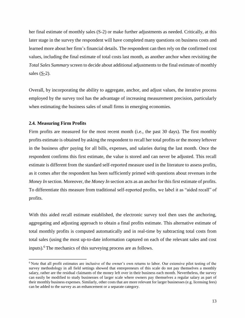
her final estimate of monthly sales (S-2) or make further adjustments as needed. Critically, at this

later stage in the survey the respondent will have completed many questions on business costs and

learned more about her firm’s financial details. The respondent can then rely on the confirmed cost

values, including the final estimate of total costs last month, as another anchor when revisiting the

Total Sales Summary screen to decide about additional adjustments to the final estimate of monthly

sales (S-2).

Overall, by incorporating the ability to aggregate, anchor, and adjust values, the iterative process

employed by the survey tool has the advantage of increasing measurement precision, particularly

when estimating the business sales of small firms in emerging economies.

2.4. Measuring Firm Profits

Firm profits are measured for the most recent month (i.e., the past 30 days). The first monthly

profits estimate is obtained by asking the respondent to recall her total profits or the money leftover

in the business after paying for all bills, expenses, and salaries during the last month. Once the

respondent confirms this first estimate, the value is stored and can never be adjusted. This recall

estimate is different from the standard self-reported measure used in the literature to assess profits,

as it comes after the respondent has been sufficiently primed with questions about revenues in the

Money In section. Moreover, the Money In section acts as an anchor for this first estimate of profits.

To differentiate this measure from traditional self-reported profits, we label it as “aided recall” of

profits.

With this aided recall estimate established, the electronic survey tool then uses the anchoring,

aggregating and adjusting approach to obtain a final profits estimate. This alternative estimate of

total monthly profits is computed automatically and in real-time by subtracting total costs from

total sales (using the most up-to-date information captured on each of the relevant sales and cost

inputs).6 The mechanics of this surveying process are as follows.

6 Note that all profit estimates are inclusive of the owner’s own returns to labor. Our extensive pilot testing of the

survey methodology in all field settings showed that entrepreneurs of this scale do not pay themselves a monthly

salary, rather are the residual claimants of the money left over in their business each month. Nevertheless, the survey

can easily be modified to study businesses of larger scale where owners pay themselves a regular salary as part of

their monthly business expenses. Similarly, other costs that are more relevant for larger businesses (e.g. licensing fees)

can be added to the survey as an enhancement or a separate category.

14

First, to construct financial records from scratch and obtain relevant anchors (for subsequent

adjustment of firm profits), respondents are required to systematically build estimates for 13 major

cost categories (i.e., high-level mental accounts). At the start of the Money Out section, the survey

instructions clearly define what is meant by firm costs: “In the next section, we are going to ask

you some questions about all the money that went out of your business in the last month (past 30

days). Please remember to focus on all of the money you spent in your business to pay for bills,

expenses, and salaries in the past 30 days.” Each of the major cost categories is represented as a

separate section in the electronic survey tool.

Next, one at a time, each major cost category is divided into its relevant sub-categories (i.e., low-

level mental accounts) with detailed questions used to obtain how much money was spent last

month on individual cost components. Particular attention is paid to getting an accurate measure

of both the amount and the frequency (e.g., daily, weekly, monthly) of each sub-category of costs.

This subdivision of costs helps correct any mismatch in timing of when costs are incurred relative

to their corresponding revenue stream. The disaggregated components are then automatically

converted into monthly values and aggregated up to create an estimate for that category’s total

monthly cost. Once all sub-category estimates (i.e., component costs) are obtained, then a within

category Major Cost Summary screen is displayed on the survey interface (see Figures 4 and 5 for

examples on Materials and Communication costs, respectively).

The respondent is prompted to review a table listing the monthly values for each sub-category as

well as the aggregated estimate of the overall category’s total cost last month. At this juncture, the

respondent can confirm her final estimate of the category’s total monthly cost or return to any of

the previous cost questions to make further adjustments. After any adjustments, the respondent

returns to the Major Cost Summary screen, reviews the updated cost information, and confirms her

final cost estimate or continues to make adjustments. The survey only proceeds to the next section

after the respondent confirms her final monthly estimate for the major cost category. It is through

this intra-category anchoring, aggregating and adjusting that a final estimate is obtained for each

of the 13 major cost categories outlined below.

15

• C-1 (stock/inventory): purchases of stock and inventory for resale – subcategories include

smallest, recent, largest, and typical purchase amounts.

• C-2 (materials/supplies): purchases of materials and supplies used as inputs into production

– subcategories include smallest, recent, largest, and typical purchase amounts.

• C-3 (employees): wages and salaries paid to people who work in the business –

subcategories include full-time employees, part-time employees, and business partners.

• C-4 (location): costs associated with operating from the business premises – subcategories

include rent, lease, and mortgage.

• C-5 (loans): payments made to service debts – subcategories include bank, microfinance

institute, moneylender, family/friends, and other.

• C-6 (energy): payments made on energy expenses – subcategories include electricity,

power generator, and other.

• C-7 (transport): money spent on transportation and travel expenses – subcategories include

travel to/from work, transport of people and assets, and loading/unloading of goods.

• C-8 (equipment): money spent on equipment and machinery – subcategories include rental

fees and repair costs.

• C-9 (food): costs related to food and water – subcategories include food (while at work

only) and water (for consumption or production).

• C-10 (phone): money spent on communication related expenses – subcategories include

mobile phone (e.g., airtime for work calls) and other communication (e.g., internet,

landlines).

• C-11 (services): money spent on business services – subcategories include marketing,

financial, legal, and other.

• C-12 (fees): payments of extra fees for the business – subcategories include taxes,

registration, insurance, and tips.

• C-13 (other): any other costs related to the business – subcategories include other1 and

other2.

Subsequently, all 13 of the major cost categories are aggregated (summed together) to compute

the total amount of money that left the business during the last month (the past 30 days).

Specifically, these 13 monthly cost estimates are stored and presented to the respondent on a

16

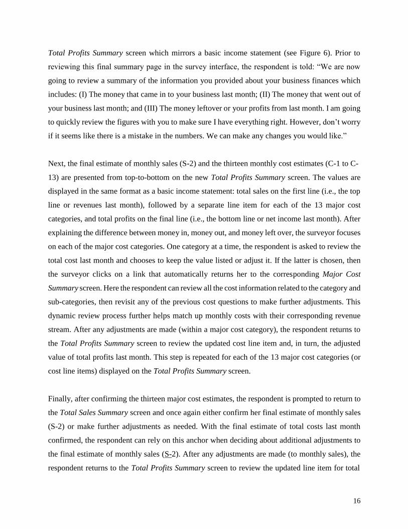
Total Profits Summary screen which mirrors a basic income statement (see Figure 6). Prior to

reviewing this final summary page in the survey interface, the respondent is told: “We are now

going to review a summary of the information you provided about your business finances which

includes: (I) The money that came in to your business last month; (II) The money that went out of

your business last month; and (III) The money leftover or your profits from last month. I am going

to quickly review the figures with you to make sure I have everything right. However, don’t worry

if it seems like there is a mistake in the numbers. We can make any changes you would like.”

Next, the final estimate of monthly sales (S-2) and the thirteen monthly cost estimates (C-1 to C-

13) are presented from top-to-bottom on the new Total Profits Summary screen. The values are

displayed in the same format as a basic income statement: total sales on the first line (i.e., the top

line or revenues last month), followed by a separate line item for each of the 13 major cost

categories, and total profits on the final line (i.e., the bottom line or net income last month). After

explaining the difference between money in, money out, and money left over, the surveyor focuses

on each of the major cost categories. One category at a time, the respondent is asked to review the

total cost last month and chooses to keep the value listed or adjust it. If the latter is chosen, then

the surveyor clicks on a link that automatically returns her to the corresponding Major Cost

Summary screen. Here the respondent can review all the cost information related to the category and

sub-categories, then revisit any of the previous cost questions to make further adjustments. This

dynamic review process further helps match up monthly costs with their corresponding revenue

stream. After any adjustments are made (within a major cost category), the respondent returns to

the Total Profits Summary screen to review the updated cost line item and, in turn, the adjusted

value of total profits last month. This step is repeated for each of the 13 major cost categories (or

cost line items) displayed on the Total Profits Summary screen.

Finally, after confirming the thirteen major cost estimates, the respondent is prompted to return to

the Total Sales Summary screen and once again either confirm her final estimate of monthly sales

(S-2) or make further adjustments as needed. With the final estimate of total costs last month

confirmed, the respondent can rely on this anchor when deciding about additional adjustments to

the final estimate of monthly sales (S-2). After any adjustments are made (to monthly sales), the

respondent returns to the Total Profits Summary screen to review the updated line item for total

17

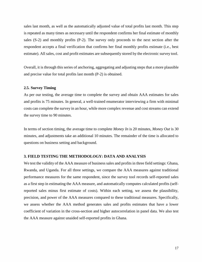
sales last month, as well as the automatically adjusted value of total profits last month. This step

is repeated as many times as necessary until the respondent confirms her final estimate of monthly

sales (S-2) and monthly profits (P-2). The survey only proceeds to the next section after the

respondent accepts a final verification that confirms her final monthly profits estimate (i.e., best

estimate). All sales, cost and profit estimates are subsequently stored by the electronic survey tool.

Overall, it is through this series of anchoring, aggregating and adjusting steps that a more plausible

and precise value for total profits last month (P-2) is obtained.

2.5. Survey Timing

As per our testing, the average time to complete the survey and obtain AAA estimates for sales

and profits is 75 minutes. In general, a well-trained enumerator interviewing a firm with minimal

costs can complete the survey in an hour, while more complex revenue and cost streams can extend

the survey time to 90 minutes.

In terms of section timing, the average time to complete Money In is 20 minutes, Money Out is 30

minutes, and adjustments take an additional 10 minutes. The remainder of the time is allocated to

questions on business setting and background.

3. FIELD TESTING THE METHODOLOGY: DATA AND ANALYSIS

We test the validity of the AAA measure of business sales and profits in three field settings: Ghana,

Rwanda, and Uganda. For all three settings, we compare the AAA measures against traditional

performance measures for the same respondent, since the survey tool records self-reported sales

as a first step in estimating the AAA measure, and automatically computes calculated profits (self-

reported sales minus first estimate of costs). Within each setting, we assess the plausibility,

precision, and power of the AAA measures compared to these traditional measures. Specifically,

we assess whether the AAA method generates sales and profits estimates that have a lower

coefficient of variation in the cross-section and higher autocorrelation in panel data. We also test

the AAA measure against unaided self-reported profits in Ghana.

18

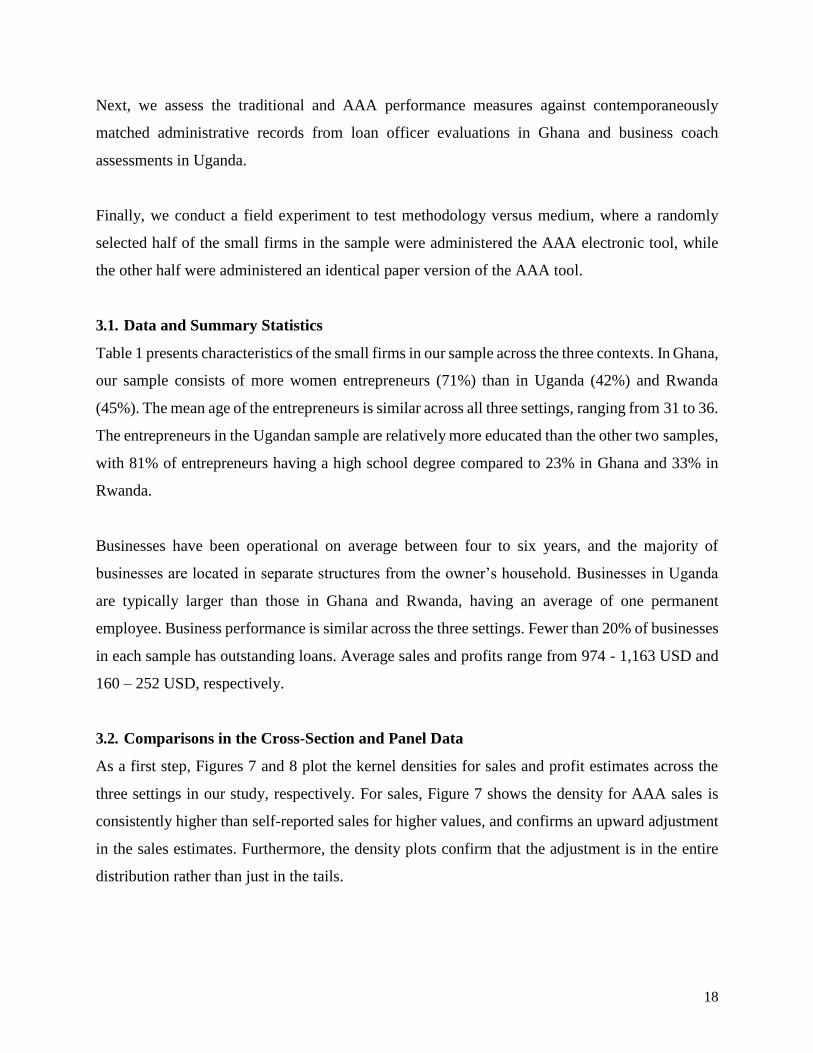
Next, we assess the traditional and AAA performance measures against contemporaneously

matched administrative records from loan officer evaluations in Ghana and business coach

assessments in Uganda.

Finally, we conduct a field experiment to test methodology versus medium, where a randomly

selected half of the small firms in the sample were administered the AAA electronic tool, while

the other half were administered an identical paper version of the AAA tool.

3.1. Data and Summary Statistics

Table 1 presents characteristics of the small firms in our sample across the three contexts. In Ghana,

our sample consists of more women entrepreneurs (71%) than in Uganda (42%) and Rwanda

(45%). The mean age of the entrepreneurs is similar across all three settings, ranging from 31 to 36.

The entrepreneurs in the Ugandan sample are relatively more educated than the other two samples,

with 81% of entrepreneurs having a high school degree compared to 23% in Ghana and 33% in

Rwanda.

Businesses have been operational on average between four to six years, and the majority of

businesses are located in separate structures from the owner’s household. Businesses in Uganda

are typically larger than those in Ghana and Rwanda, having an average of one permanent

employee. Business performance is similar across the three settings. Fewer than 20% of businesses

in each sample has outstanding loans. Average sales and profits range from 974 - 1,163 USD and

160 – 252 USD, respectively.

3.2. Comparisons in the Cross-Section and Panel Data

As a first step, Figures 7 and 8 plot the kernel densities for sales and profit estimates across the

three settings in our study, respectively. For sales, Figure 7 shows the density for AAA sales is

consistently higher than self-reported sales for higher values, and confirms an upward adjustment

in the sales estimates. Furthermore, the density plots confirm that the adjustment is in the entire

distribution rather than just in the tails.

19

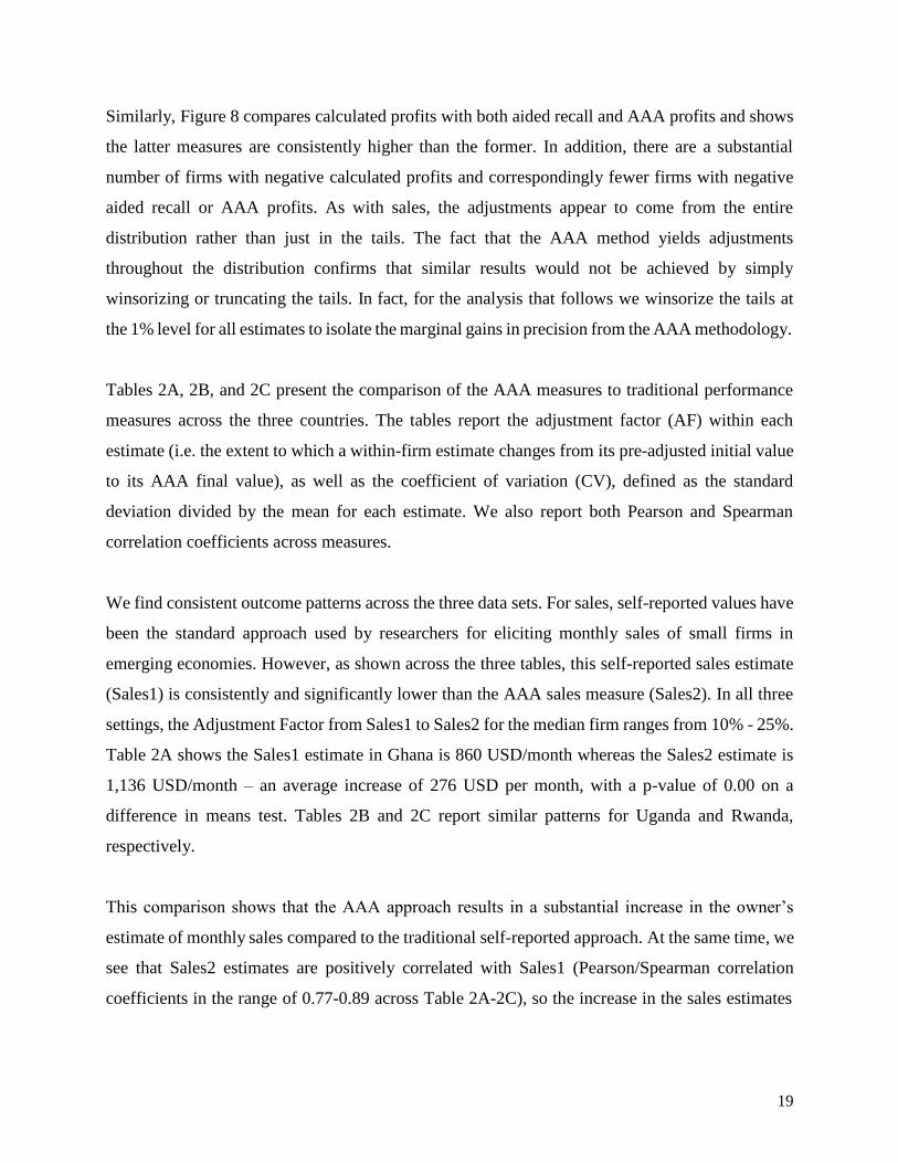
Similarly, Figure 8 compares calculated profits with both aided recall and AAA profits and shows

the latter measures are consistently higher than the former. In addition, there are a substantial

number of firms with negative calculated profits and correspondingly fewer firms with negative

aided recall or AAA profits. As with sales, the adjustments appear to come from the entire

distribution rather than just in the tails. The fact that the AAA method yields adjustments

throughout the distribution confirms that similar results would not be achieved by simply

winsorizing or truncating the tails. In fact, for the analysis that follows we winsorize the tails at

the 1% level for all estimates to isolate the marginal gains in precision from the AAA methodology.

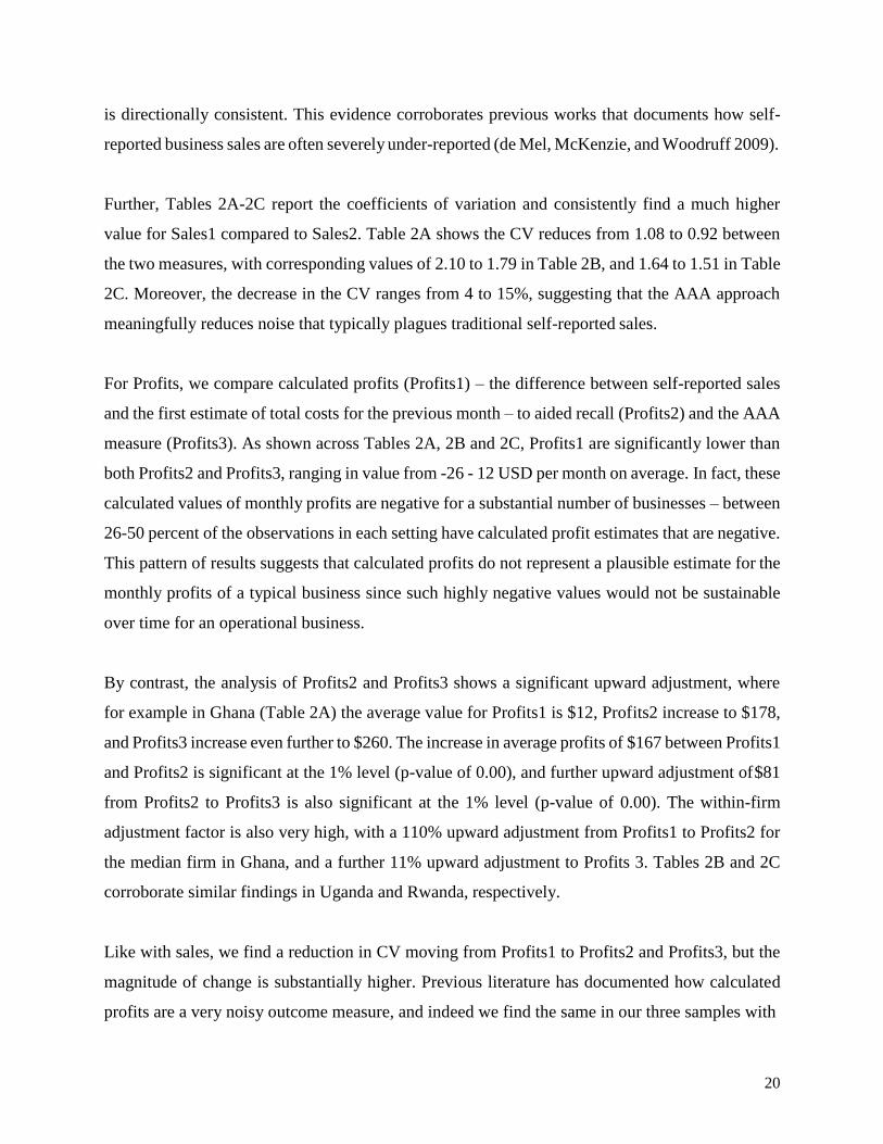
Tables 2A, 2B, and 2C present the comparison of the AAA measures to traditional performance

measures across the three countries. The tables report the adjustment factor (AF) within each

estimate (i.e. the extent to which a within-firm estimate changes from its pre-adjusted initial value

to its AAA final value), as well as the coefficient of variation (CV), defined as the standard

deviation divided by the mean for each estimate. We also report both Pearson and Spearman

correlation coefficients across measures.

We find consistent outcome patterns across the three data sets. For sales, self-reported values have

been the standard approach used by researchers for eliciting monthly sales of small firms in

emerging economies. However, as shown across the three tables, this self-reported sales estimate

(Sales1) is consistently and significantly lower than the AAA sales measure (Sales2). In all three

settings, the Adjustment Factor from Sales1 to Sales2 for the median firm ranges from 10% - 25%.

Table 2A shows the Sales1 estimate in Ghana is 860 USD/month whereas the Sales2 estimate is

1,136 USD/month – an average increase of 276 USD per month, with a p-value of 0.00 on a

difference in means test. Tables 2B and 2C report similar patterns for Uganda and Rwanda,

respectively.

This comparison shows that the AAA approach results in a substantial increase in the owner’s

estimate of monthly sales compared to the traditional self-reported approach. At the same time, we

see that Sales2 estimates are positively correlated with Sales1 (Pearson/Spearman correlation

coefficients in the range of 0.77-0.89 across Table 2A-2C), so the increase in the sales estimates

20

is directionally consistent. This evidence corroborates previous works that documents how self-

reported business sales are often severely under-reported (de Mel, McKenzie, and Woodruff 2009).

Further, Tables 2A-2C report the coefficients of variation and consistently find a much higher

value for Sales1 compared to Sales2. Table 2A shows the CV reduces from 1.08 to 0.92 between

the two measures, with corresponding values of 2.10 to 1.79 in Table 2B, and 1.64 to 1.51 in Table

2C. Moreover, the decrease in the CV ranges from 4 to 15%, suggesting that the AAA approach

meaningfully reduces noise that typically plagues traditional self-reported sales.

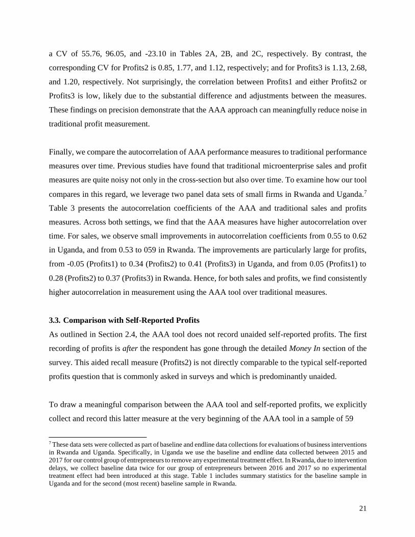
For Profits, we compare calculated profits (Profits1) – the difference between self-reported sales

and the first estimate of total costs for the previous month – to aided recall (Profits2) and the AAA

measure (Profits3). As shown across Tables 2A, 2B and 2C, Profits1 are significantly lower than

both Profits2 and Profits3, ranging in value from -26 - 12 USD per month on average. In fact, these

calculated values of monthly profits are negative for a substantial number of businesses – between

26-50 percent of the observations in each setting have calculated profit estimates that are negative.

This pattern of results suggests that calculated profits do not represent a plausible estimate for the

monthly profits of a typical business since such highly negative values would not be sustainable

over time for an operational business.

By contrast, the analysis of Profits2 and Profits3 shows a significant upward adjustment, where

for example in Ghana (Table 2A) the average value for Profits1 is $12, Profits2 increase to $178,

and Profits3 increase even further to $260. The increase in average profits of $167 between Profits1

and Profits2 is significant at the 1% level (p-value of 0.00), and further upward adjustment of $81

from Profits2 to Profits3 is also significant at the 1% level (p-value of 0.00). The within-firm

adjustment factor is also very high, with a 110% upward adjustment from Profits1 to Profits2 for

the median firm in Ghana, and a further 11% upward adjustment to Profits 3. Tables 2B and 2C

corroborate similar findings in Uganda and Rwanda, respectively.

Like with sales, we find a reduction in CV moving from Profits1 to Profits2 and Profits3, but the

magnitude of change is substantially higher. Previous literature has documented how calculated

profits are a very noisy outcome measure, and indeed we find the same in our three samples with

21

a CV of 55.76, 96.05, and -23.10 in Tables 2A, 2B, and 2C, respectively. By contrast, the

corresponding CV for Profits2 is 0.85, 1.77, and 1.12, respectively; and for Profits3 is 1.13, 2.68,

and 1.20, respectively. Not surprisingly, the correlation between Profits1 and either Profits2 or

Profits3 is low, likely due to the substantial difference and adjustments between the measures.

These findings on precision demonstrate that the AAA approach can meaningfully reduce noise in

traditional profit measurement.

Finally, we compare the autocorrelation of AAA performance measures to traditional performance

measures over time. Previous studies have found that traditional microenterprise sales and profit

measures are quite noisy not only in the cross-section but also over time. To examine how our tool

compares in this regard, we leverage two panel data sets of small firms in Rwanda and Uganda.7

Table 3 presents the autocorrelation coefficients of the AAA and traditional sales and profits

measures. Across both settings, we find that the AAA measures have higher autocorrelation over

time. For sales, we observe small improvements in autocorrelation coefficients from 0.55 to 0.62

in Uganda, and from 0.53 to 059 in Rwanda. The improvements are particularly large for profits,

from -0.05 (Profits1) to 0.34 (Profits2) to 0.41 (Profits3) in Uganda, and from 0.05 (Profits1) to

0.28 (Profits2) to 0.37 (Profits3) in Rwanda. Hence, for both sales and profits, we find consistently

higher autocorrelation in measurement using the AAA tool over traditional measures.

3.3. Comparison with Self-Reported Profits

As outlined in Section 2.4, the AAA tool does not record unaided self-reported profits. The first

recording of profits is after the respondent has gone through the detailed Money In section of the

survey. This aided recall measure (Profits2) is not directly comparable to the typical self-reported

profits question that is commonly asked in surveys and which is predominantly unaided.

To draw a meaningful comparison between the AAA tool and self-reported profits, we explicitly

collect and record this latter measure at the very beginning of the AAA tool in a sample of 59

7 These data sets were collected as part of baseline and endline data collections for evaluations of business interventions

in Rwanda and Uganda. Specifically, in Uganda we use the baseline and endline data collected between 2015 and

2017 for our control group of entrepreneurs to remove any experimental treatment effect. In Rwanda, due to intervention

delays, we collect baseline data twice for our group of entrepreneurs between 2016 and 2017 so no experimental

treatment effect had been introduced at this stage. Table 1 includes summary statistics for the baseline sample in

Uganda and for the second (most recent) baseline sample in Rwanda.

22

entrepreneurs in Ghana.8 Specifically, before we take the respondents through any questions about

their business performance, we ask them to give their best estimate of business profits for the most

recent month after accounting for all business revenues and costs. Moreover, the question on

recalled profits is shifted to the very beginning of the survey rather than after the Money In section.

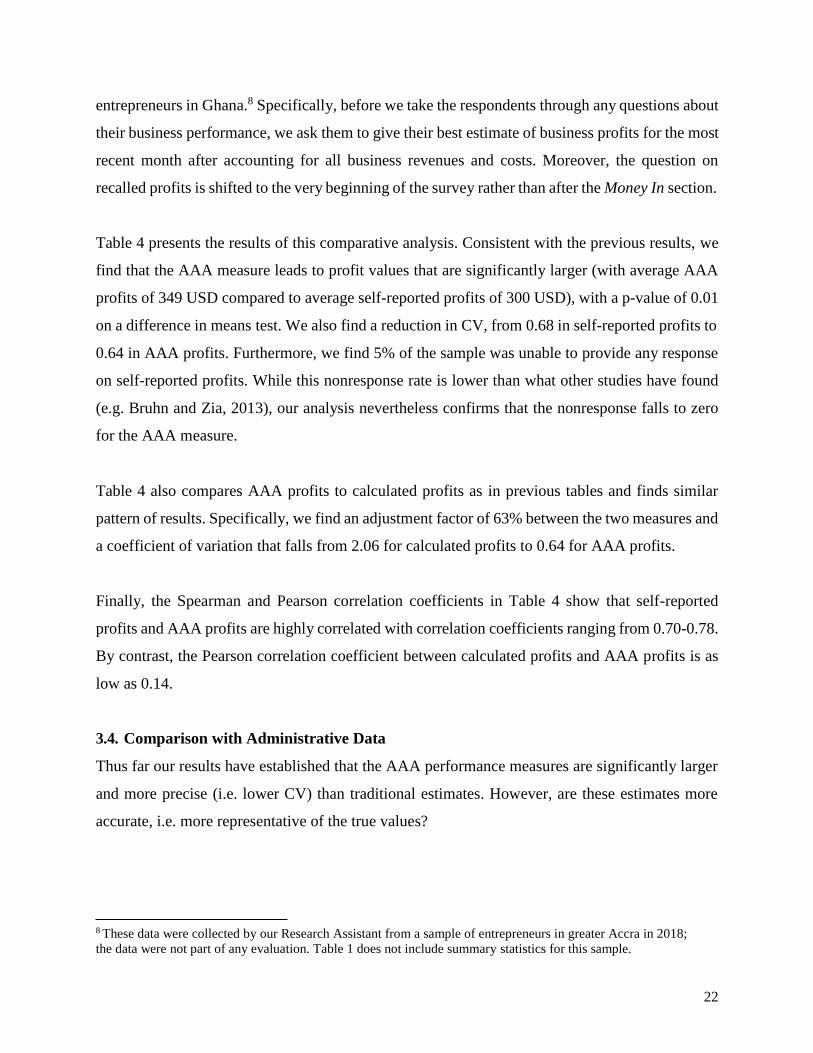
Table 4 presents the results of this comparative analysis. Consistent with the previous results, we

find that the AAA measure leads to profit values that are significantly larger (with average AAA

profits of 349 USD compared to average self-reported profits of 300 USD), with a p-value of 0.01

on a difference in means test. We also find a reduction in CV, from 0.68 in self-reported profits to

0.64 in AAA profits. Furthermore, we find 5% of the sample was unable to provide any response

on self-reported profits. While this nonresponse rate is lower than what other studies have found

(e.g. Bruhn and Zia, 2013), our analysis nevertheless confirms that the nonresponse falls to zero

for the AAA measure.

Table 4 also compares AAA profits to calculated profits as in previous tables and finds similar

pattern of results. Specifically, we find an adjustment factor of 63% between the two measures and

a coefficient of variation that falls from 2.06 for calculated profits to 0.64 for AAA profits.

Finally, the Spearman and Pearson correlation coefficients in Table 4 show that self-reported

profits and AAA profits are highly correlated with correlation coefficients ranging from 0.70-0.78.

By contrast, the Pearson correlation coefficient between calculated profits and AAA profits is as

low as 0.14.

3.4. Comparison with Administrative Data

Thus far our results have established that the AAA performance measures are significantly larger

and more precise (i.e. lower CV) than traditional estimates. However, are these estimates more

accurate, i.e. more representative of the true values?

8 These data were collected by our Research Assistant from a sample of entrepreneurs in greater Accra in 2018;

the data were not part of any evaluation. Table 1 does not include summary statistics for this sample.

23

Given most small businesses in developing economies do not keep formal (or any) financial

records and administrative data are predominantly unavailable or expensive to collect, it is difficult

to determine with certainty what the true value is for sales and profits in the previous month. In

this subsection, we explicitly seek out administrative data on businesses across two samples for

which we contemporaneously collect AAA data. In this manner, we can directly compare the

magnitude and CV of AAA measures against administrative records.

The two sources of administrate data are loan officer evaluation files in Ghana and professional

business coach assessments in Uganda. In Ghana, we identify 50 small firms from a partner bank’s

database that had financial statements prepared within the last month by the bank’s loan officers.

We complete the AAA performance tool with these 50 firms for the same reporting period and

reference month as the financial statements in order to directly compare our performance measures

to the administrative data. In Uganda, we use data from an intervention in which professional

coaches mentored businesses in our study for 12 comprehensive sessions over a six-month period.

In the final session, the consultants were asked to assess the financial performance of the

businesses and generate estimates for monthly sales and profits. We compare the coaches’

estimates to the estimates generated from our survey tool for the same reporting period and

reference month for 31 firms for which we have data. Firms were not privy to either the loan officer

evaluations or the professional coach assessments, so their responses to the AAA survey

instrument were not influenced by prior knowledge from these sources.9

Tables 5A and 5B presents the results of this analysis and show very similar findings in Ghana and

Uganda, respectively. For sales, the AAA estimates and administrative estimates are statistically

indistinguishable in both settings, although the magnitude of administrative sales is larger. In fact,

the CV is lower for the AAA measure, with a value of 0.86 compared to 1.07 in Ghana; and 1.58

compared to 2.01 in Uganda. Hence, AAA sales match administrative sales very well across two

sources of administrative data.

9 Note that both sample sizes are small because we were limited in matching the same reference month across

administrative data and the AAA survey.

24

For profits, we find comparable results that the magnitude is higher in administrative data than in

the AAA tool, but the difference in this case is statistically significant for Ghana. However, the

difference in magnitudes is not statistically different in Uganda. Overall, these findings confirm

that if we believe administrative data to be the closest “true” business performance indicator, then

the AAA tool comes very close to matching it in terms of magnitude and precision. Note that all

traditional measures of sales and profits have significantly lower magnitude than AAA estimates

with AAA sales of 1,608 USD and 1,306 USD in Ghana and Uganda compared to 1,384 USD and

1,205 USD, respectively; and AAA profits of 374 USD and 215 USD in Ghana and Uganda

compared to 245 USD and 92 USD, respectively.

Furthermore, as discussed earlier administrative data for the vast majority of small firms in

developing countries simply does not exist and would be very expensive and time-consuming to

collect. In comparison, the AAA methodology provides a compelling alternative, offering

comparable value much more efficiently and cheaply.

3.5. Method or Medium?

As a final test of the validity of the AAA tool, we explicitly conduct a field experiment in Ghana

to assess the measurement methodology. Specifically, we randomly assign half the survey

respondents from a baseline business survey the AAA electronic tool and the other half an identical

paper version of the tool.10 Both survey instruments include the same set of questions and steps for

measuring firm sales and profits. All surveyors received identical training and each surveyor

implemented the electronic tool or the paper tool to a respondent on a randomized basis; each

surveyor was randomly assigned 50% electronic instruments and 50% paper instruments to

complete (thus the only thing that differed was the 'approach' of using an electronic tool). This

approach allows us to examine differences between the questioning techniques (reported versus

anchored/adjusted) while isolating any effects due to the electronic tool versus paper tool.

Moreover, by comparing outcomes across the two versions of the tool, we can differentiate

whether gains in precision are attributable to the medium of conducting surveys (electronic versus

paper) or to the AAA method.

10 Table 1 includes summary statistics for the sample that was assigned the electronic version of the AAA tool.

25

Table 5 compares sales and profits measures across the two mediums. Overall, there are similar

patterns of results for each medium with no statistically significant differences across the two.

Specifically, we find that moving from a self-reported or calculated measure to the corresponding

AAA measure leads to more plausible (i.e. larger) figures for both sales and profits. Furthermore,

the AAA measures are more precise for both mediums. We find a marginal decrease in the CVs

moving from a self-reported sales measure to the AAA sales measure and a substantial decrease

in CVs moving from a calculated profits measure to the AAA profits measure. Finally, we do not

find significant differences between the two mediums across all estimates; average monthly sales

and profits estimates are comparable regardless of whether collected via the paper or electronic

tool. These results affirm that it is the AAA methodology and not the electronic medium that leads

to improvements in sales and profits measures.

3.6. AAA “Light”

The preceding sections present multiple pieces of evidence on how the AAA measurement

methodology improves both the precision and accuracy of business outcomes over traditional

measures. The analysis shows AAA sales are larger in magnitude, have lower coefficient of

variation, and are closer to administrative sales as compared to traditional self-reported sales. The

same pattern is present for profits; however, the methodology produces two measures for profits,

aided recall (Profits2) and the AAA estimate (Profits3). The comparison between these two

estimates offers a meaningful choice in survey design and implementation. On the one hand, tables

2A, 2B, and 2C consistently show that the AAA estimate (Profits3) is significantly higher than

aided recall (Profits2) across all settings, and this measure is the closest match to administrative

records as shown in Tables 5A and 5B. As such, the AAA value is the most accurate estimate of

“true” firm profits.

On the other hand, the analysis also shows that both aided recall and AAA estimates reduce the

CV substantially from Profits1, have high autocorrelation coefficients, and are also highly

correlated with each other (Pearson coefficient range: 0.58-0.81; Spearman coefficient range: 0.63-

0.82). Furthermore, the aided recall measure saves at least 30 minutes of survey time. Hence,

researchers with binding budget constraints or limited capacity to implement the full AAA survey

methodology can still achieve many of the gains in measurement precision by measuring AAA

26

sales and then relying on the aided recall measure of profits. This “light” version of the survey

further highlights the adaptability of the AAA methodology.

4. CONCLUSION

This paper presents a new business survey methodology designed to address the challenges that

often plague measurement of microenterprise financials, including underreporting, implausible

figures, high variance, and low autocorrelation over time. The survey tool combines automatic

consistency checks of electronic data collection with real-time adjustments in reported outcomes

to generate more precise estimates for business financial outcomes. This new methodological

approach and survey tool represent an innovative and cost-effective way to gather accurate

performance data on micro and small businesses in countries and settings where administrative

data are unavailable.

This survey methodology is valuable for policy makers, researchers, and businesses alike. A key

challenge to advancing private enterprise development lies in accurately being able to measure

which policies and programs work (or not) to enhance business outcomes. The AAA methodology

offers a reliable mechanism in this regard. The tool also provides a way for researchers to better

understand small firms. As de Mel, McKenzie, and Woodruff note, “we need a much more nuanced

and detailed understanding of [micro and small entrepreneurs] before appropriate policies can be

devised” (2010, p.25). And one of the building blocks to developing this understanding is accurate

measurement of business outcomes, which can help identify and rank growth constraints across

firms.

Finally, improvements in entrepreneurial outcomes would provide a way of “helping people help

themselves” (Nopo 2007, p.2). Once shown to be effective as a research tool, this technology could

be provided directly to individual entrepreneurs as a way to improve their record keeping and to

access business intelligence (e.g., by converting it into a simple smartphone app). Furthermore,

this methodology could be leveraged to create user-friendly tools designed to increase a firm

owner’s ability to track, access, and take action on business intelligence.

27

REFERENCES

Abebe, Girum. 2013. “Recall Bias in Retrospective Surveys: Evidence from Enterprise-Level

Data.” Asian-African Journal of Economics and Econometrics 13(1): 17-33.

Antonides, Gerrit., I. Manon de Groot, and W. Fred van Raaij. 2011. “Mental Budgeting and the

Management of Household Finance.” Journal of Economic Psychology 32(4): 546-555.

Beatty, Paul. 2010. “Considerations Regarding the Use of Global Survey Questions.” Presentation

at the Consumer Expenditures Survey Methods Workshop, December 8-9, 2010, Suitland, MD

Beegle, Kathleen, Joachim De Weerdt, Jed Friedman, and John Gibson. 2012. "Methods of

Household Consumption Measurement Through Surveys: Experimental Results From Tanzania,"

Journal of Development Economics 98(1): 3-18.

Belli, Robert, Norbert Schwartz, Eleanor Singer, and Jennifer Talarico. 2000. “Decomposition Can

Harm the Accuracy of Behavioral Frequency Reports.” Applied Cognitive Psychology 14(4): 295-

308.

Blair, Edward, and Scott Burton. 1987. “Cognitive Processes Used by Survey Respondents to

Answer Behavioral Frequency Questions.” Journal of Consumer Research 14(2): 280-288.

Chapman, Gretchen B., and Eric J. Johnson. 2002. “Incorporating the Irrelevant: Anchors in

Judgments of Belief and Value.” In T. Gilovich, D. Griffin, & D. Kahneman (Eds.), Heuristics and

Biases: The Psychology of Intuitive Judgment (pp. 120-138). Cambridge, UK: Cambridge

University Press.

Chapman, Gretchen B., and Eric J. Johnson. 1994. “The Limits of Anchoring.” Journal of

Behavioral Decision Making 7(4): 223-242.

Chapman, Gretchen B., and Eric J. Johnson. 1999. “Anchoring, Activation and the Construction

of Value.” Organizational Behavior and Human Decision Processes 79(2): 115-153.

Collins, Daryl, Jonathan Morduch, and Stuart Rutherford. 2009. Portfolios of the Poor: How the

World's Poor Live on $2 a Day. Princeton, NJ: Princeton University Press.

Daniels, Lisa. 2001. “Testing Alternative Measures of Microenterprise Profits and Net Worth.”

Journal of International Development 13: 599–614.

De Mel, Suresh, David McKenzie, and Christopher Woodruff. 2009. “Measuring Microenterprise

Profits: Must We Ask How the Sausage is Made?” Journal of Development Economics 88(1): 19–

31.

De Mel, Suresh, Dammika Herath, David McKenzie, and Yuvraj Pathak. 2016. “Radio Frequency

(Un)Identification Results from a Proof-of-Concept Trial of the Use of RFID Technology to

Measure Microenterprise Turnover in Sri Lanka.” Development Engineering 1(1): 4-11.

28

De Nicola, Francesca, and Xavier Giné. 2014. “How Accurate are Recall Data? Evidence from

Coastal India.” Journal of Development Economics 1(106): 52-65.

Deaton, Angus, and Margaret Grosh. 2000. “Consumption.” In Margaret Grosh and

Paul Glewwe (Eds.), “Designing Household Survey Questionnaires for Developing Countries:

Lessons from 15 Years of the Living Standards Measurement Study.” World Bank, Washington,

D.C.

Drexler, Alejandro, Greg Fischer, and Antoinette Schoar. 2014. “Keeping it Simple: Financial

Literacy and Rules of Thumb.” American Economic Journal: Applied Economics, 6(2): 1-31.

Dupas, Pascaline, and Jonathan Robinson. 2013. “Savings Constraints and Microenterprise

Development: Evidence from a Field Experiment in Kenya.” American Economic Journal:

Applied Economics 5(1): 163-192.

Epley, Nicholas, and Thomas Gilovich. 2004. “Are Adjustments Insufficient?” Personality and

Social Psychology Bulletin 30: 447–460.

Epley, Nicholas, and Thomas Gilovich. 2001. “Putting Adjustment Back in the Anchoring and

Adjustment Heuristic: Differential Processing of Self-Generated and Experimenter-Provided

Anchors.” Psychological Science 12(5): 391–396.

Fafchamps, Marcel, David McKenzie, Simon Quinn, and Christopher Woodruff. 2012. “Using

PDA Consistency Checks to Increase the Precision of Profits and Sales Measurement in Panels.”

Journal of Development Economics 98(1): 51-57.

Garlick, Robert, Kate Orkin, and Simon Quinn. 2016. “Call Me Maybe: Experimental Evidence

on Using Mobile Phones to Survey Microenterprises.” Economic Research Initiatives at Duke

(ERID) Working Paper No. 224.

Gibson, John. 2006. “Statistical Tools and Estimation Methods for Poverty Measures Based on

Cross-Sectional Household Surveys.” In: Jonathan Morduch (Ed.), “Handbook on Poverty

Statistics.” United Nations Statistics Division (2006).

Gilbert, Daniel T., Brett W. Pelham, and Douglas S. Krull. 1988. On Cognitive Busyness: When

Person Perceivers Meet Persons Perceived. Journal of Personality & Social Psychology 54(5):

733-740.

Heath, Chip, and Jack B. Soll. 1996. “Mental Budgeting and Consumer Decisions.” Journal of

Consumer Research 23(1): 40-52.

Kahneman, Daniel, and Amos Tversky. 1974. “Judgement Under Uncertainty: Heuristics and

Biases.” Science 185(4157): 1124-1131.

29

Kahneman, Daniel, and Amos Tversky. 1979. “Prospect Theory: An Analysis of Decision Under

Risk.” Econometrica 47(2): 263-291.

Keysar, Boaz, Dale J. Barr, and Jennifer A. Balin, and Jason S. Brauner. 2000. “Taking Perspective

in Conversation: The Role of Mutual Knowledge in Comprehension.” Psychological Science

11(1): 32-38.

Klinger, Bailey, and Matthias Schündeln. 2011. “Can Entrepreneurial Activity be Taught? Quasi-

Experimental Evidence from Central America.” World Development 39(9): 1592–610.

Liedholm, Carl. 1991. “Data Collection Strategies for Small-scale Industry Surveys.” GEMINI

Working Paper No. 11, Bethesda, MD: Development Alternatives Inc.

McKenzie, David. 2012. “Beyond Baseline and Follow-up: The Case for more T in Experiments.”

Journal of Development Economics 99(1): 210-221.

McKenzie, David, and Christopher Woodruff. 2014. “What Are We Learning from Business

Training and Entrepreneurship Evaluations Around the Developing World?” World Bank

Research Observer 29(1): 48-82.

Menon, Geeta. 1997. “Are the Parts Better than the Whole? The Effects of Decompositional

Questions on Judgments of Frequent Behaviors.” Journal of Marketing Research 34: 335-346.

Milkman, Katherine L., and John Beshears. 2009. “Mental Accounting and Small Windfalls:

Evidence from and Online Grocer.” Journal of Economic Behavior & Organization 71(2): 384-

393.

Prelec, Drazen, and George Loewenstein. 1998. “The Red and the Black: Mental Accounting of

Savings and Debt.” Marketing Science 17(1): 4-28.

Quattrone, George A. 1982. “Overattribution and Unit Formation: When Behavior Engulfs the

Person.” Journal of Personality and Social Psychology 42(4): 593-607.

Quattrone, George A., C.P. Lawrence, S.E. Finkel, and D.C. Andrus. 1981. Explorations in

Anchoring: The Effects of Prior Range, Anchor Extremity, and Suggestive hints. Unpublished

manuscript, Stanford University, Stanford, CA.

Samphantharak, Krislert, and Robert M. Townsend. 2012. “Measuring the Return on Household

Enterprise: What Matters Most for Whom?” Journal of Development Economics 98(1): 58–70.

Samphantharak, Krislert, and Robert M. Townsend. 2006. “Households as Corporate Firms:

Constructing Financial Statements from Integrated Household Surveys”, Mimeo. UCSD and

University of Chicago.

30

Schwarz, Norbert. 199. “Assessing Frequency Reports of Mundane Behaviors: Contributions of

Cognitive Psychology to Questionnaire Construction.” In C. Hendrick and M. S. Clark (Eds.),

Research Methods in Personality and Social Psychology (pp. 98–119). Beverly Hills, CA: Sage.

Strack, Fritz, and Thomas Mussweiler. 1997. “Explaining the Enigmatic Anchoring Affect:

Mechanisms of Selective Accessibility.” Journal of Personality and Social Psychology 73(3): 437-

446.

Strube, Gerhard. 1987. “Answering Survey Questions: The Role of Memory.” In H. J. Hippler, N.

Schwarz and S. Sudman (Eds.), Social Information Processing and Survey Methodology (pp. 86–

101). New York: Springer-Verlag.

Sudman, Seymour, Norman Bradburn, and Norbert Schwarz. 1996. Thinking About Answers: The

Application of Cognitive Processes to Survey Methodology. San Francisco, CA: Jossey-Bass.

Thaler, Richard. 1985. “Mental Accounting and Consumer Choice.” Marketing Science 4(3): 199

– 214.

Thaler, Richard. 1999. “Mental Accounting Matters.” Journal of Behavioral Decision Making 12:

183-206.

Thaler, Richard, and H.M. Shefrin. 1981. “An Economic Theory of Self-Control.” Journal of

Political Economy 89(2): 392-406.

Tulving, Endel. 1972. “Episodic and Semantic Memory.” In E. Tulving and W. Donaldson (Eds.),

Organization of Memory (pp. 382-402). New York: Academic Press.

Valdivia, Martin. 2012. “Training or Technical Assistance for Female Entrepreneurship? Evidence

from a Field Experiment in Peru.” Mimeo. GRADE.

Vijverberg, W. P. (1992). Measuring income from family enterprises with household surveys.

Small Business Economics. 4(4): 287-305.

Vijverberg, Wim P.M., and Donald Mead. 2000. Household Enterprises. In Grosh, Margaret, and

Paul Glewwe (Eds.), Designing Household Survey Questionnaires for Developing Countries:

Lessons from 15 years of the Living Standards Measurement Survey, Vol. 2 (pp. 105–137). The

World Bank, Washington, DC.

Wilson, Timothy D., Christopher E. Houston, Kathryn M. Etling, and Nancy Brekke. 1996. “A

New Look at Anchoring Effects: Basic Anchoring and Its Antecedents.” Journal of Experimental

Psychology: General 125(4): 387-402.

31

Figure 1: Weekly Sales Recall Page

32

Figure 2: Daily Sales Recall Page

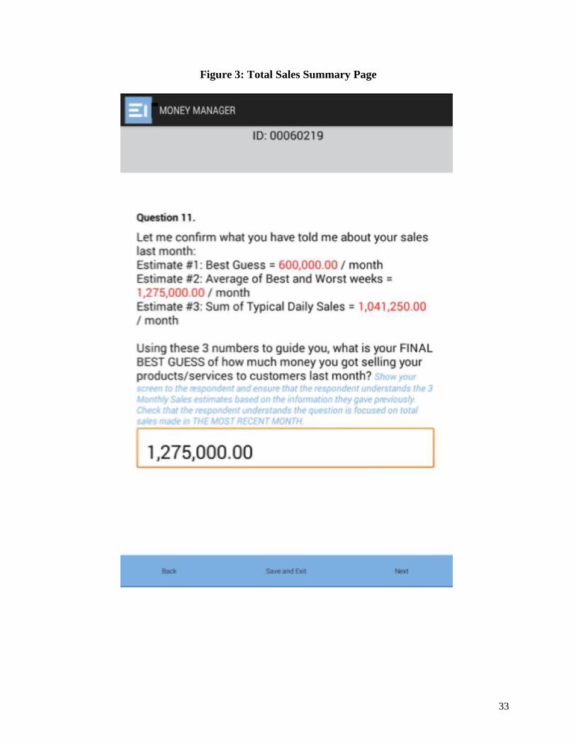
33

Figure 3: Total Sales Summary Page

34

Figure 4: Materials/Supplies Costs Summary Page

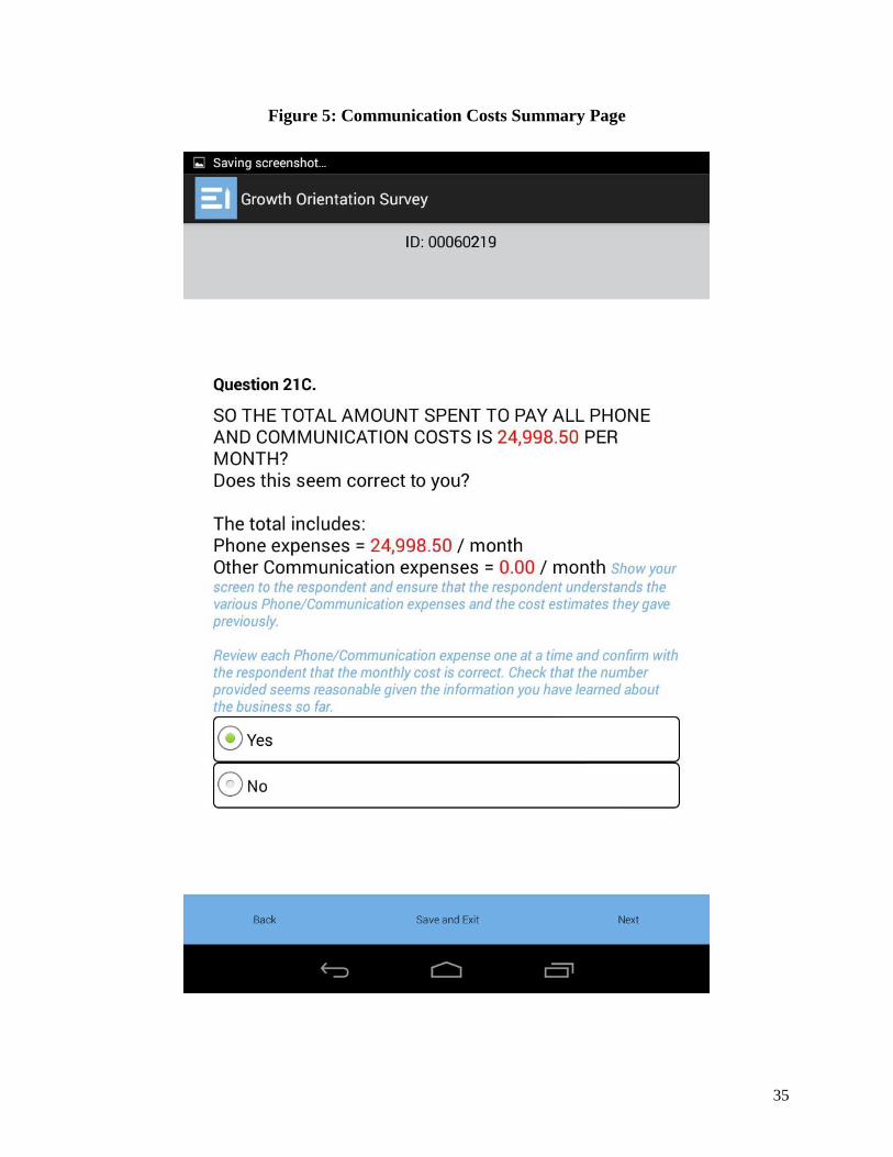
35

Figure 5: Communication Costs Summary Page

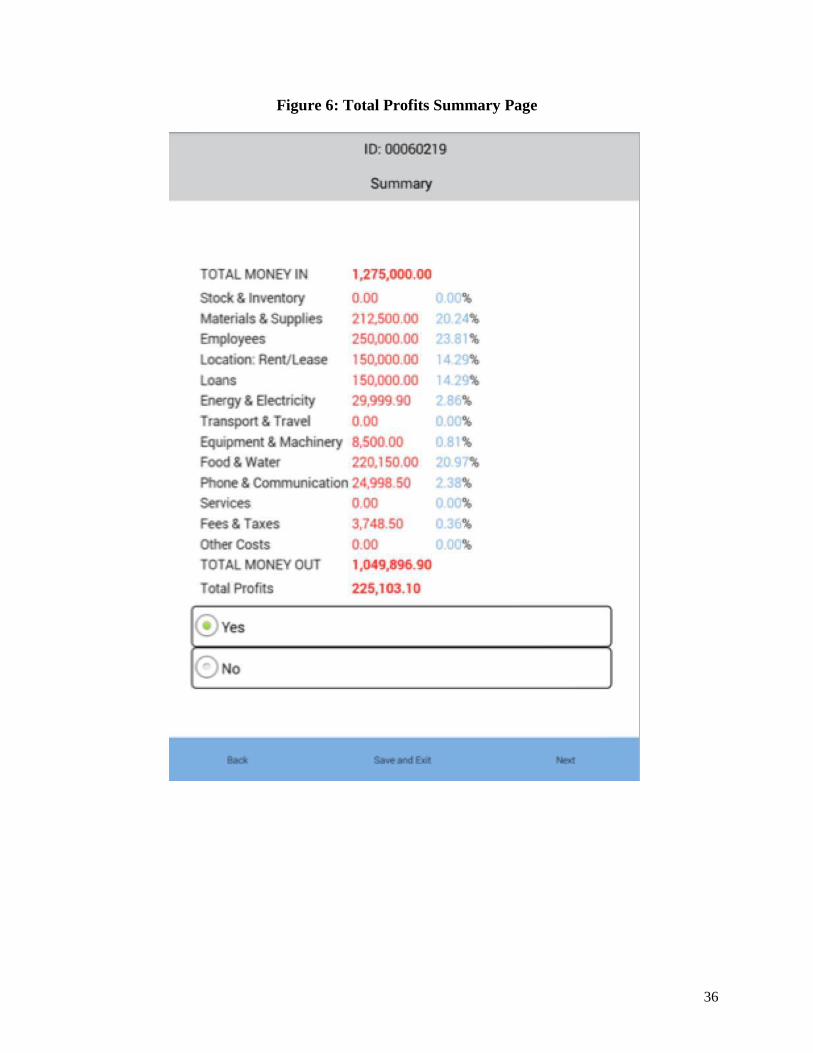
36

Figure 6: Total Profits Summary Page

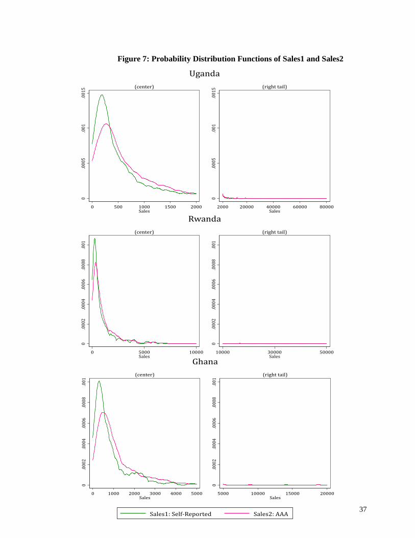
37

Figure 7: Probability Distribution Functions of Sales1 and Sales2

0.0005

.001

.0015

0 500 1000 1500 2000Sales

(center)

0.0005

.001

.0015

2000 20000 40000 60000 80000Sales

(righttail)

Uganda

Sales1:Self-Reported Sales2:AAA

0.0002

.0004

.0006

.0008

.001

0 5000 10000Sales

(center)

0.0002

.0004

.0006

.0008

.001

10000 30000 50000Sales

(righttail)

Rwanda

Sales1:Self-Reported Sales2:AAA

0.0002

.0004

.0006

.0008

.001

0 1000 2000 3000 4000 5000Sales

(center)

0.0002

.0004

.0006

.0008

.001

5000 10000 15000 20000Sales

(righttail)

Ghana

Sales1:Self-Reported Sales2:AAA

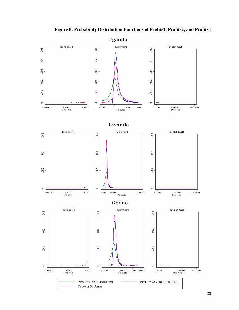
38

Figure 8: Probability Distribution Functions of Profits1, Profits2, and Profits3

0.001

.002

.003

.004

.005

-10000 -5000 -500Pro, its

(lefttail)

0.001

.002

.003

.004

.005

-500 0 500 1000Pro, its

(center)

0.001

.002

.003

.004

.005

1000 20000 40000Pro, its

(righttail)

Uganda

Pro, its1:Calculated Pro, its2:AidedRecall

Pro, its3:AAA

0.001

.002

.003

-10000 -5000 -500Pro+its

(lefttail)

0.001

.002

.003

-1000 0 1000 2000 3000Pro+its

(center)

0.001

.002

.003

2500 25000 40000Pro+its

(righttail)

Ghana

Pro+its1:Calculated Pro+its2:AidedRecall

Pro+its3:AAA

0.002

.004

.006

-10000 -5000 -500Pro, its

(lefttail)

0.002

.004

.006

-500 1000 5000Pro, its

(center)

0.002

.004

.006

5000 10000 15000Pro, its

(righttail)

Rwanda

Pro, its1:Calculated Pro, its2:AidedRecall

Pro, its3:AAA

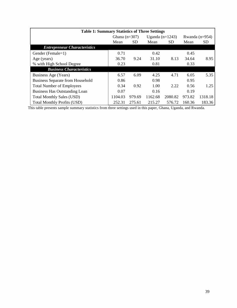
39

Table 1: Summary Statistics of Three Settings

Ghana (n=307) Uganda (n=1243) Rwanda (n=954) Mean SD Mean SD Mean SD

Entrepreneur Characteristics

Gender (Female=1) 0.71 0.42 0.45

Age (years) 36.70 9.24 31.10 8.13 34.64 8.95

% with High School Degree 0.23 0.81 0.33

Business Characteristics

Business Age (Years) 6.57 6.09 4.25 4.71 6.05 5.35

Business Separate from Household 0.86 0.98 0.95

Total Number of Employees 0.34 0.92 1.00 2.22 0.56 1.25

Business Has Outstanding Loan 0.07 0.16 0.19

Total Monthly Sales (USD) 1104.03 979.69 1162.68 2080.82 973.82 1318.18

Total Monthly Profits (USD) 252.31 275.61 215.27 576.72 160.36 183.36

This table presents sample summary statistics from three settings used in this paper, Ghana, Uganda, and Rwanda.

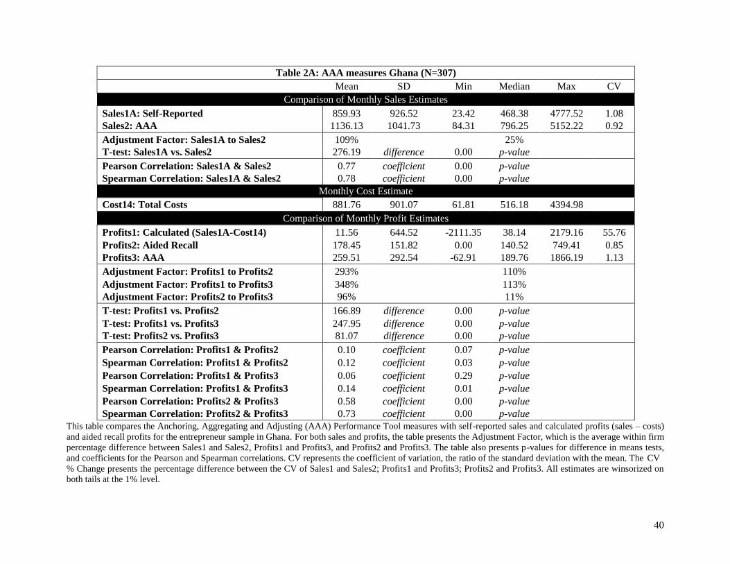
40

Table 2A: AAA measures Ghana (N=307)

Mean SD Min Median Max CV

Comparison of Monthly Sales Estimates

Sales1A: Self-Reported 859.93 926.52 23.42 468.38 4777.52 1.08

Sales2: AAA 1136.13 1041.73 84.31 796.25 5152.22 0.92

Adjustment Factor: Sales1A to Sales2 109% 25%

T-test: Sales1A vs. Sales2 276.19 difference 0.00 p-value

Pearson Correlation: Sales1A & Sales2 0.77 coefficient 0.00 p-value

Spearman Correlation: Sales1A & Sales2 0.78 coefficient 0.00 p-value

Monthly Cost Estimate

Cost14: Total Costs 881.76 901.07 61.81 516.18 4394.98

Comparison of Monthly Profit Estimates

Profits1: Calculated (Sales1A-Cost14) 11.56 644.52 -2111.35 38.14 2179.16 55.76

Profits2: Aided Recall 178.45 151.82 0.00 140.52 749.41 0.85

Profits3: AAA 259.51 292.54 -62.91 189.76 1866.19 1.13

Adjustment Factor: Profits1 to Profits2 293% 110%

Adjustment Factor: Profits1 to Profits3 348% 113%

Adjustment Factor: Profits2 to Profits3 96% 11%

T-test: Profits1 vs. Profits2 166.89 difference 0.00 p-value

T-test: Profits1 vs. Profits3 247.95 difference 0.00 p-value

T-test: Profits2 vs. Profits3 81.07 difference 0.00 p-value

Pearson Correlation: Profits1 & Profits2 0.10 coefficient 0.07 p-value

Spearman Correlation: Profits1 & Profits2 0.12 coefficient 0.03 p-value

Pearson Correlation: Profits1 & Profits3 0.06 coefficient 0.29 p-value

Spearman Correlation: Profits1 & Profits3 0.14 coefficient 0.01 p-value

Pearson Correlation: Profits2 & Profits3 0.58 coefficient 0.00 p-value

Spearman Correlation: Profits2 & Profits3 0.73 coefficient 0.00 p-value

This table compares the Anchoring, Aggregating and Adjusting (AAA) Performance Tool measures with self-reported sales and calculated profits (sales – costs)

and aided recall profits for the entrepreneur sample in Ghana. For both sales and profits, the table presents the Adjustment Factor, which is the average within firm

percentage difference between Sales1 and Sales2, Profits1 and Profits3, and Profits2 and Profits3. The table also presents p-values for difference in means tests,

and coefficients for the Pearson and Spearman correlations. CV represents the coefficient of variation, the ratio of the standard deviation with the mean. The CV

% Change presents the percentage difference between the CV of Sales1 and Sales2; Profits1 and Profits3; Profits2 and Profits3. All estimates are winsorized on

both tails at the 1% level.

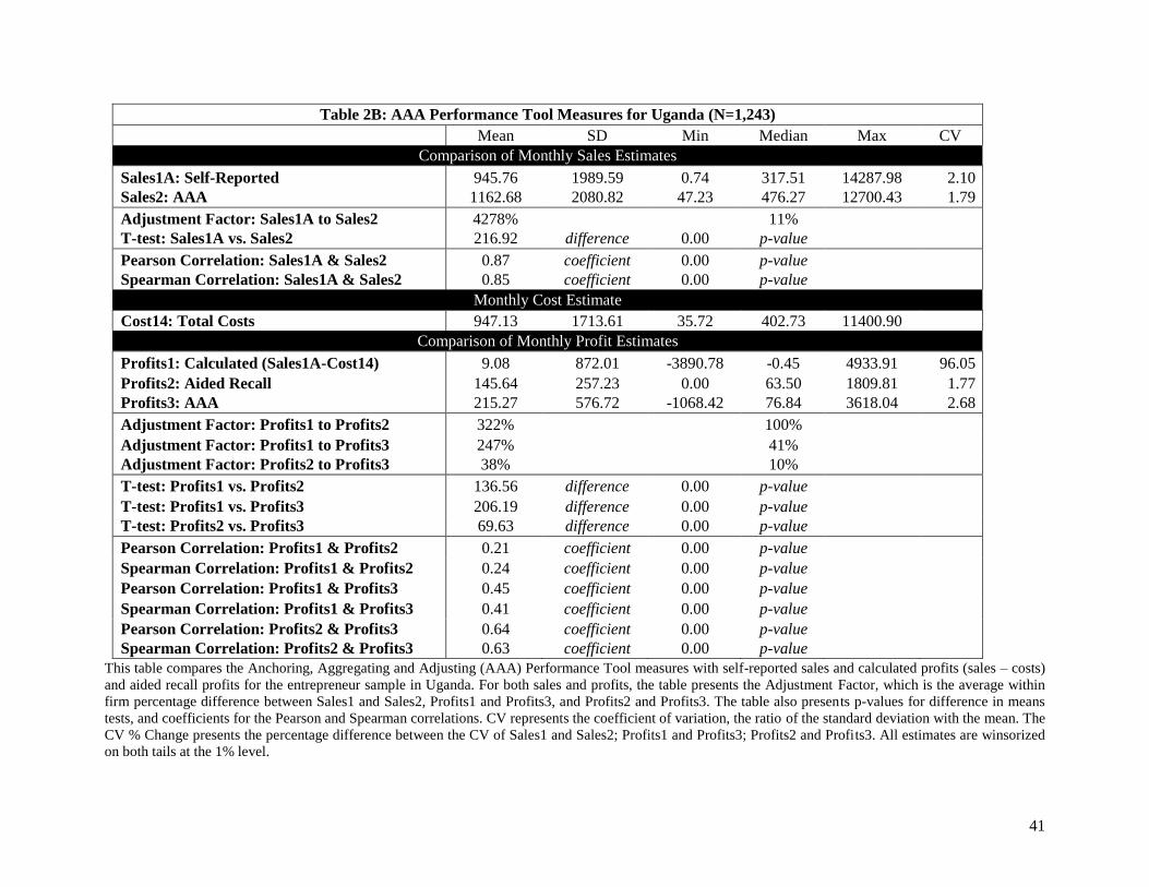
41

Table 2B: AAA Performance Tool Measures for Uganda (N=1,243)

Mean SD Min Median Max CV

Comparison of Monthly Sales Estimates

Sales1A: Self-Reported 945.76 1989.59 0.74 317.51 14287.98 2.10

Sales2: AAA 1162.68 2080.82 47.23 476.27 12700.43 1.79

Adjustment Factor: Sales1A to Sales2 4278% 11%

T-test: Sales1A vs. Sales2 216.92 difference 0.00 p-value

Pearson Correlation: Sales1A & Sales2 0.87 coefficient 0.00 p-value

Spearman Correlation: Sales1A & Sales2 0.85 coefficient 0.00 p-value

Monthly Cost Estimate

Cost14: Total Costs 947.13 1713.61 35.72 402.73 11400.90

Comparison of Monthly Profit Estimates

Profits1: Calculated (Sales1A-Cost14) 9.08 872.01 -3890.78 -0.45 4933.91 96.05

Profits2: Aided Recall 145.64 257.23 0.00 63.50 1809.81 1.77

Profits3: AAA 215.27 576.72 -1068.42 76.84 3618.04 2.68

Adjustment Factor: Profits1 to Profits2 322% 100%

Adjustment Factor: Profits1 to Profits3 247% 41%

Adjustment Factor: Profits2 to Profits3 38% 10%

T-test: Profits1 vs. Profits2 136.56 difference 0.00 p-value

T-test: Profits1 vs. Profits3 206.19 difference 0.00 p-value

T-test: Profits2 vs. Profits3 69.63 difference 0.00 p-value

Pearson Correlation: Profits1 & Profits2 0.21 coefficient 0.00 p-value

Spearman Correlation: Profits1 & Profits2 0.24 coefficient 0.00 p-value

Pearson Correlation: Profits1 & Profits3 0.45 coefficient 0.00 p-value

Spearman Correlation: Profits1 & Profits3 0.41 coefficient 0.00 p-value

Pearson Correlation: Profits2 & Profits3 0.64 coefficient 0.00 p-value

Spearman Correlation: Profits2 & Profits3 0.63 coefficient 0.00 p-value

This table compares the Anchoring, Aggregating and Adjusting (AAA) Performance Tool measures with self-reported sales and calculated profits (sales – costs)

and aided recall profits for the entrepreneur sample in Uganda. For both sales and profits, the table presents the Adjustment Factor, which is the average within

firm percentage difference between Sales1 and Sales2, Profits1 and Profits3, and Profits2 and Profits3. The table also presents p-values for difference in means

tests, and coefficients for the Pearson and Spearman correlations. CV represents the coefficient of variation, the ratio of the standard deviation with the mean. The

CV % Change presents the percentage difference between the CV of Sales1 and Sales2; Profits1 and Profits3; Profits2 and Profits3. All estimates are winsorized

on both tails at the 1% level.

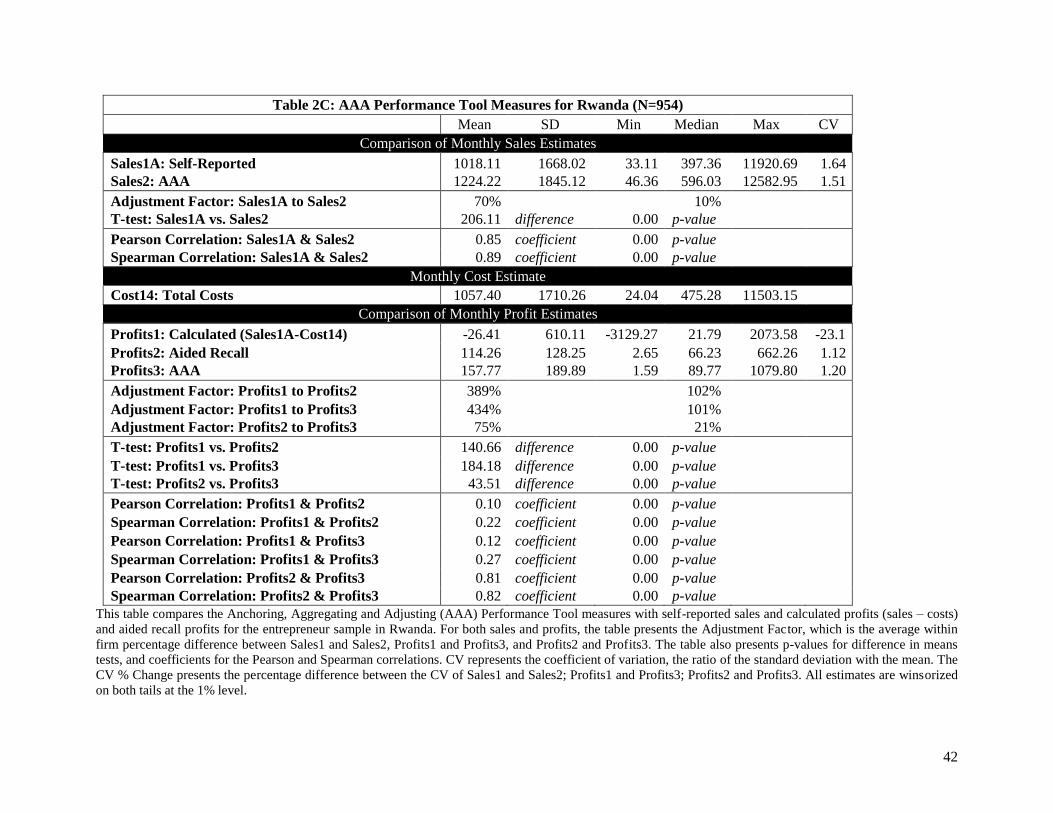
42

Table 2C: AAA Performance Tool Measures for Rwanda (N=954)

Mean SD Min Median Max CV

Comparison of Monthly Sales Estimates

Sales1A: Self-Reported 1018.11 1668.02 33.11 397.36 11920.69 1.64

Sales2: AAA 1224.22 1845.12 46.36 596.03 12582.95 1.51

Adjustment Factor: Sales1A to Sales2 70% 10%

T-test: Sales1A vs. Sales2 206.11 difference 0.00 p-value

Pearson Correlation: Sales1A & Sales2 0.85 coefficient 0.00 p-value

Spearman Correlation: Sales1A & Sales2 0.89 coefficient 0.00 p-value

Monthly Cost Estimate

Cost14: Total Costs 1057.40 1710.26 24.04 475.28 11503.15

Comparison of Monthly Profit Estimates

Profits1: Calculated (Sales1A-Cost14) -26.41 610.11 -3129.27 21.79 2073.58 -23.1

Profits2: Aided Recall 114.26 128.25 2.65 66.23 662.26 1.12

Profits3: AAA 157.77 189.89 1.59 89.77 1079.80 1.20

Adjustment Factor: Profits1 to Profits2 389% 102%

Adjustment Factor: Profits1 to Profits3 434% 101%

Adjustment Factor: Profits2 to Profits3 75% 21%

T-test: Profits1 vs. Profits2 140.66 difference 0.00 p-value

T-test: Profits1 vs. Profits3 184.18 difference 0.00 p-value

T-test: Profits2 vs. Profits3 43.51 difference 0.00 p-value

Pearson Correlation: Profits1 & Profits2 0.10 coefficient 0.00 p-value

Spearman Correlation: Profits1 & Profits2 0.22 coefficient 0.00 p-value

Pearson Correlation: Profits1 & Profits3 0.12 coefficient 0.00 p-value

Spearman Correlation: Profits1 & Profits3 0.27 coefficient 0.00 p-value

Pearson Correlation: Profits2 & Profits3 0.81 coefficient 0.00 p-value

Spearman Correlation: Profits2 & Profits3 0.82 coefficient 0.00 p-value

This table compares the Anchoring, Aggregating and Adjusting (AAA) Performance Tool measures with self-reported sales and calculated profits (sales – costs)

and aided recall profits for the entrepreneur sample in Rwanda. For both sales and profits, the table presents the Adjustment Factor, which is the average within

firm percentage difference between Sales1 and Sales2, Profits1 and Profits3, and Profits2 and Profits3. The table also presents p-values for difference in means

tests, and coefficients for the Pearson and Spearman correlations. CV represents the coefficient of variation, the ratio of the standard deviation with the mean. The

CV % Change presents the percentage difference between the CV of Sales1 and Sales2; Profits1 and Profits3; Profits2 and Profits3. All estimates are winsorized

on both tails at the 1% level.

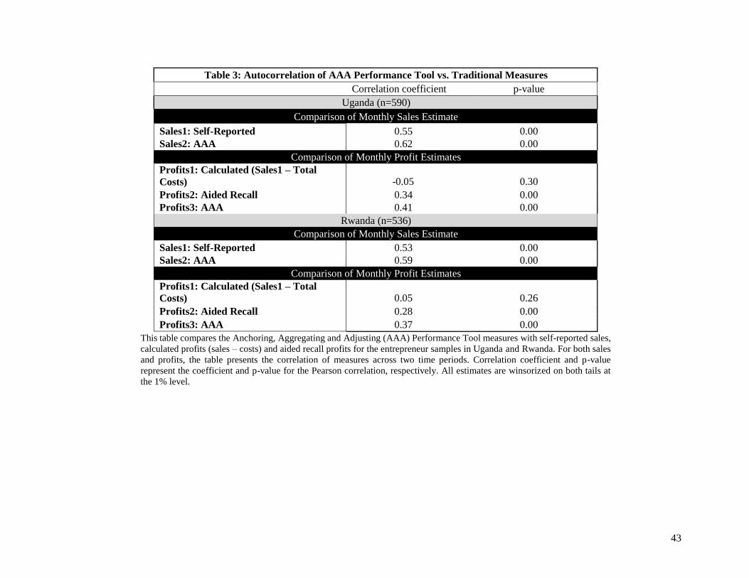
43

Table 3: Autocorrelation of AAA Performance Tool vs. Traditional Measures

Correlation coefficient p-value

Uganda (n=590)

Comparison of Monthly Sales Estimate

Sales1: Self-Reported 0.55 0.00

Sales2: AAA 0.62 0.00

Comparison of Monthly Profit Estimates

Profits1: Calculated (Sales1 – Total

Costs)

-0.05

0.30

Profits2: Aided Recall 0.34 0.00

Profits3: AAA 0.41 0.00

Rwanda (n=536)

Comparison of Monthly Sales Estimate

Sales1: Self-Reported 0.53 0.00

Sales2: AAA 0.59 0.00

Comparison of Monthly Profit Estimates

Profits1: Calculated (Sales1 – Total

Costs)

0.05

0.26

Profits2: Aided Recall 0.28 0.00

Profits3: AAA 0.37 0.00

This table compares the Anchoring, Aggregating and Adjusting (AAA) Performance Tool measures with self-reported sales,

calculated profits (sales – costs) and aided recall profits for the entrepreneur samples in Uganda and Rwanda. For both sales

and profits, the table presents the correlation of measures across two time periods. Correlation coefficient and p-value

represent the coefficient and p-value for the Pearson correlation, respectively. All estimates are winsorized on both tails at

the 1% level.

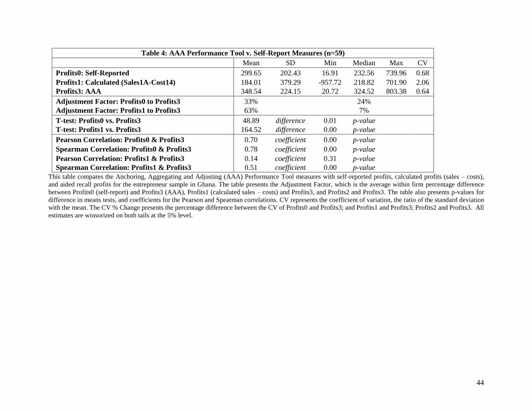
44

Table 4: AAA Performance Tool v. Self-Report Measures (n=59)

Mean SD Min Median Max CV

Profits0: Self-Reported 299.65 202.43 16.91 232.56 739.96 0.68

Profits1: Calculated (Sales1A-Cost14) 184.01 379.29 -957.72 218.82 701.90 2.06

Profits3: AAA 348.54 224.15 20.72 324.52 803.38 0.64

Adjustment Factor: Profits0 to Profits3 33% 24%

Adjustment Factor: Profits1 to Profits3 63% 7%

T-test: Profits0 vs. Profits3 48.89 difference 0.01 p-value

T-test: Profits1 vs. Profits3 164.52 difference 0.00 p-value

Pearson Correlation: Profits0 & Profits3 0.70 coefficient 0.00 p-value

Spearman Correlation: Profits0 & Profits3 0.78 coefficient 0.00 p-value

Pearson Correlation: Profits1 & Profits3 0.14 coefficient 0.31 p-value

Spearman Correlation: Profits1 & Profits3 0.51 coefficient 0.00 p-value

This table compares the Anchoring, Aggregating and Adjusting (AAA) Performance Tool measures with self-reported profits, calculated profits (sales – costs),

and aided recall profits for the entrepreneur sample in Ghana. The table presents the Adjustment Factor, which is the average within firm percentage difference

between Profits0 (self-report) and Profits3 (AAA), Profits1 (calculated sales – costs) and Profits3, and Profits2 and Profits3. The table also presents p-values for

difference in means tests, and coefficients for the Pearson and Spearman correlations. CV represents the coefficient of variation, the ratio of the standard deviation

with the mean. The CV % Change presents the percentage difference between the CV of Profits0 and Profits3; and Profits1 and Profits3; Profits2 and Profits3. All

estimates are winsorized on both tails at the 5% level.

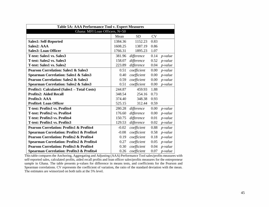
45

Table 5A: AAA Performance Tool v. Expert Measures

Ghana: MFI Loan Officers, N=50

Mean SD CV

Sales1: Self-Reported 1384.36 1152.23 0.83

Sales2: AAA 1608.25 1387.19 0.86

Sales3: Loan Officer 1766.31 1895.23 1.07

T-test: Sales1 vs. Sales3 381.96 difference 0.14 p-value

T-test: Sales2 vs. Sales3 158.07 difference 0.52 p-value

T-test: Sales1 vs. Sales2 223.89 difference 0.04 p-value

Pearson Correlation: Sales1 & Sales3 0.51 coefficient 0.00 p-value

Spearman Correlation: Sales1 & Sales3 0.40 coefficient 0.00 p-value

Pearson Correlation: Sales2 & Sales3 0.59 coefficient 0.00 p-value

Spearman Correlation: Sales2 & Sales3 0.51 coefficient 0.00 p-value

Profits1: Calculated (Sales1 – Total Costs) 244.87 459.93 1.88

Profits2: Aided Recall 348.54 254.16 0.73

Profits3: AAA 374.40 348.38 0.93

Profits4: Loan Officer 525.15 312.44 0.59

T-test: Profits1 vs. Profits4 280.28 difference 0.00 p-value

T-test: Profits2 vs. Profits4 176.60 difference 0.00 p-value

T-test: Profits3 vs. Profits4 150.75 difference 0.01 p-value

T-test: Profits1 vs. Profits3 129.53 difference 0.02 p-value

Pearson Correlation: Profits1 & Profits4 -0.02 coefficient 0.88 p-value

Spearman Correlation: Profits1 & Profits4 -0.08 coefficient 0.58 p-value

Pearson Correlation: Profits2 & Profits4 0.19 coefficient 0.18 p-value

Spearman Correlation: Profits2 & Profits4 0.27 coefficient 0.05 p-value

Pearson Correlation: Profits3 & Profits4 0.30 coefficient 0.04 p-value

Spearman Correlation: Profits3 & Profits4 0.26 coefficient 0.07 p-value

This table compares the Anchoring, Aggregating and Adjusting (AAA) Performance Tool sales/profits measures with

self-reported sales, calculated profits, aided recall profits and loan officer sales/profits measures for the entrepreneur

sample in Ghana. The table presents p-values for difference in means tests, and coefficients for the Pearson and

Spearman correlations. CV represents the coefficient of variation, the ratio of the standard deviation with the mean.

The estimates are winsorized on both tails at the 5% level.

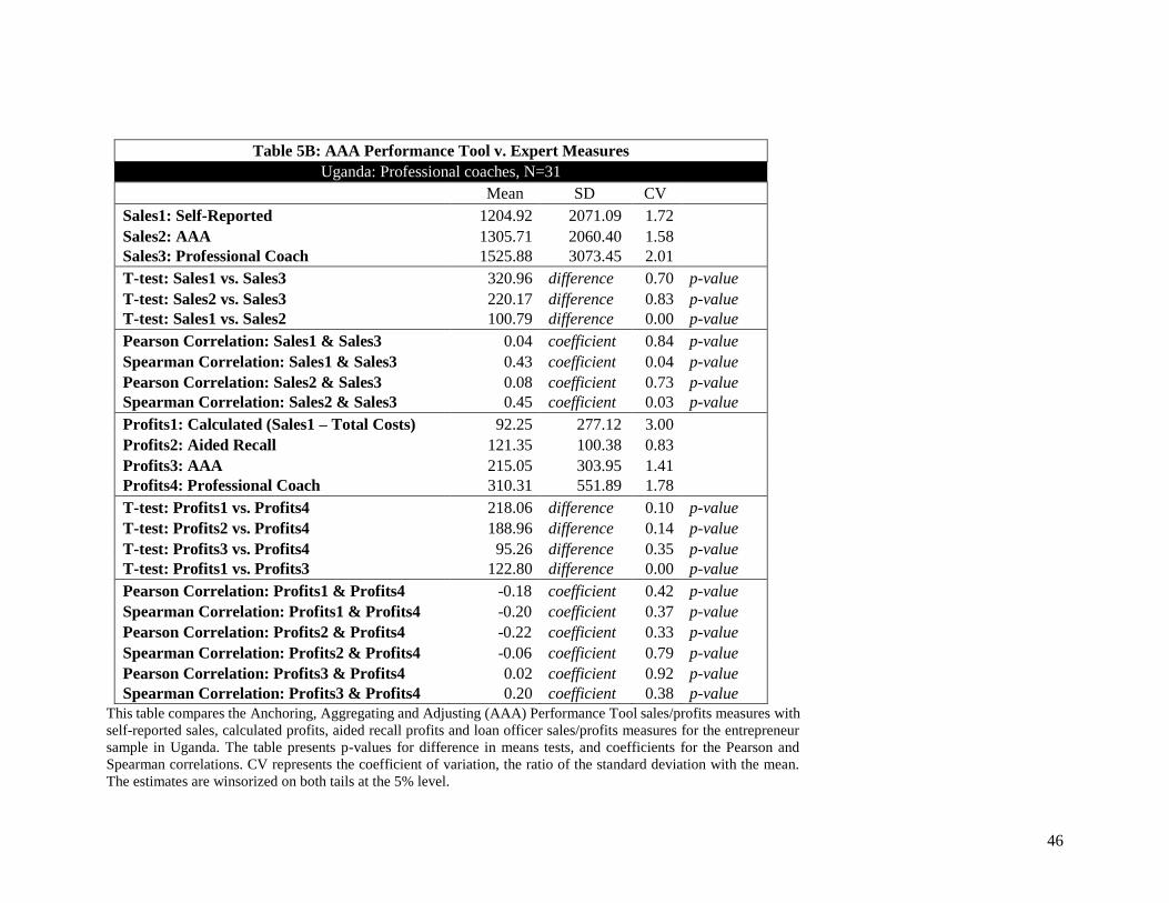
46

Table 5B: AAA Performance Tool v. Expert Measures

Uganda: Professional coaches, N=31

Mean SD CV

Sales1: Self-Reported 1204.92 2071.09 1.72

Sales2: AAA 1305.71 2060.40 1.58

Sales3: Professional Coach 1525.88 3073.45 2.01

T-test: Sales1 vs. Sales3 320.96 difference 0.70 p-value

T-test: Sales2 vs. Sales3 220.17 difference 0.83 p-value

T-test: Sales1 vs. Sales2 100.79 difference 0.00 p-value

Pearson Correlation: Sales1 & Sales3 0.04 coefficient 0.84 p-value

Spearman Correlation: Sales1 & Sales3 0.43 coefficient 0.04 p-value

Pearson Correlation: Sales2 & Sales3 0.08 coefficient 0.73 p-value

Spearman Correlation: Sales2 & Sales3 0.45 coefficient 0.03 p-value

Profits1: Calculated (Sales1 – Total Costs) 92.25 277.12 3.00

Profits2: Aided Recall 121.35 100.38 0.83

Profits3: AAA 215.05 303.95 1.41

Profits4: Professional Coach 310.31 551.89 1.78

T-test: Profits1 vs. Profits4 218.06 difference 0.10 p-value

T-test: Profits2 vs. Profits4 188.96 difference 0.14 p-value

T-test: Profits3 vs. Profits4 95.26 difference 0.35 p-value

T-test: Profits1 vs. Profits3 122.80 difference 0.00 p-value

Pearson Correlation: Profits1 & Profits4 -0.18 coefficient 0.42 p-value

Spearman Correlation: Profits1 & Profits4 -0.20 coefficient 0.37 p-value

Pearson Correlation: Profits2 & Profits4 -0.22 coefficient 0.33 p-value

Spearman Correlation: Profits2 & Profits4 -0.06 coefficient 0.79 p-value

Pearson Correlation: Profits3 & Profits4 0.02 coefficient 0.92 p-value

Spearman Correlation: Profits3 & Profits4 0.20 coefficient 0.38 p-value

This table compares the Anchoring, Aggregating and Adjusting (AAA) Performance Tool sales/profits measures with

self-reported sales, calculated profits, aided recall profits and loan officer sales/profits measures for the entrepreneur

sample in Uganda. The table presents p-values for difference in means tests, and coefficients for the Pearson and

Spearman correlations. CV represents the coefficient of variation, the ratio of the standard deviation with the mean.

The estimates are winsorized on both tails at the 5% level.

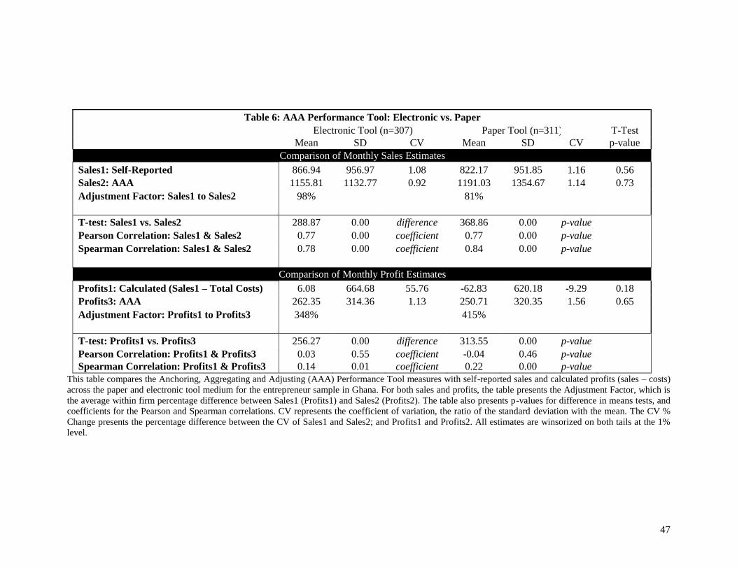
47

Table 6: AAA Performance Tool: Electronic vs. Paper

Electronic Tool (n=307) Paper Tool (n=311) T-Test Mean SD CV Mean SD CV p-value

Comparison of Monthly Sales Estimates

Sales1: Self-Reported 866.94 956.97 1.08 822.17 951.85 1.16 0.56

Sales2: AAA 1155.81 1132.77 0.92 1191.03 1354.67 1.14 0.73

Adjustment Factor: Sales1 to Sales2 98% 81%

T-test: Sales1 vs. Sales2 288.87 0.00 difference 368.86 0.00 p-value

Pearson Correlation: Sales1 & Sales2 0.77 0.00 coefficient 0.77 0.00 p-value

Spearman Correlation: Sales1 & Sales2 0.78 0.00 coefficient 0.84 0.00 p-value

Comparison of Monthly Profit Estimates

Profits1: Calculated (Sales1 – Total Costs) 6.08 664.68 55.76 -62.83 620.18 -9.29 0.18

Profits3: AAA 262.35 314.36 1.13 250.71 320.35 1.56 0.65

Adjustment Factor: Profits1 to Profits3 348% 415%

T-test: Profits1 vs. Profits3 256.27 0.00 difference 313.55 0.00 p-value

Pearson Correlation: Profits1 & Profits3 0.03 0.55 coefficient -0.04 0.46 p-value

Spearman Correlation: Profits1 & Profits3 0.14 0.01 coefficient 0.22 0.00 p-value

This table compares the Anchoring, Aggregating and Adjusting (AAA) Performance Tool measures with self-reported sales and calculated profits (sales – costs)

across the paper and electronic tool medium for the entrepreneur sample in Ghana. For both sales and profits, the table presents the Adjustment Factor, which is

the average within firm percentage difference between Sales1 (Profits1) and Sales2 (Profits2). The table also presents p-values for difference in means tests, and

coefficients for the Pearson and Spearman correlations. CV represents the coefficient of variation, the ratio of the standard deviation with the mean. The CV %

Change presents the percentage difference between the CV of Sales1 and Sales2; and Profits1 and Profits2. All estimates are winsorized on both tails at the 1%

level.