Embed Size (px)
Citation preview
Policy Research Working Paper 5339
Measuring the Technical Efficiency of Airports in Latin America
Sergio PerelmanTomas Serebrisky
The World BankLatin America and the Caribbean RegionSustainable Development DepartmentJune 2010
WPS5339P
ublic
Dis
clos
ure
Aut
horiz
edP
ublic
Dis
clos
ure
Aut
horiz
edP
ublic
Dis
clos
ure
Aut
horiz
edP
ublic
Dis
clos
ure
Aut
horiz
edP
ublic
Dis
clos
ure
Aut
horiz
edP
ublic
Dis
clos
ure
Aut
horiz
edP
ublic
Dis
clos
ure
Aut
horiz
edP
ublic
Dis
clos
ure
Aut
horiz
ed
Produced by the Research Support Team
Abstract
The Policy Research Working Paper Series disseminates the findings of work in progress to encourage the exchange of ideas about development issues. An objective of the series is to get the findings out quickly, even if the presentations are less than fully polished. The papers carry the names of the authors and should be cited accordingly. The findings, interpretations, and conclusions expressed in this paper are entirely those of the authors. They do not necessarily represent the views of the International Bank for Reconstruction and Development/World Bank and its affiliated organizations, or those of the Executive Directors of the World Bank or the governments they represent.
Policy Research Working Paper 5339
This paper studies the technical efficiency of airports in Latin America. The evolution of productive efficiency in the region has seldom been studied, mainly due to lack of publicly available data. Relying on a unique dataset that was obtained through questionnaires distributed to airport operators, the authors use Data Envelopment Analysis methods to compute an efficient production frontier and compare the technical efficiency of Latin American airports relative to airports around the world. In a second stage, they estimate a truncated regression to study the drivers of observed differences in airport efficiency. According to the results, institutional
This paper—a product of the Sustainable Development Department, Latin America and the Caribbean Region—is part of a larger effort in the department to understand the determinants of performance in the infrastructure sectors. Policy Research Working Papers are also posted on the Web at http://econ.worldbank.org. The authors may be contacted at [email protected] and [email protected].
variables (private/public operation), the socioeconomic environment (level of gross domestic product), and airport characteristics (hub airport, share of commercial revenues) matter in explaining airport productive efficiency. Finally, the authors compute total factor productivity changes for Latin American airports for 1995–2007. The region has implemented a wide variety of private sector participation schemes for the operation of airports since the mid 1990s. The results show that private operators have not had higher rates of total factor productivity change.
Measuring the Technical Efficiency of Airports in
Latin America
Sergio Perelman CREPP, University of Liege
Bd. du Rectorat 7 (B31), 4000 Liège, Belgium +32 43663098, [email protected]
Tomas Serebrisky1 The World Bank
WORLD BANK - MSN I6-601, Washington DC 20433, USA +1 202 458-2872, [email protected]
JEL classification: L25, L33, L90
1 Corresponding author: Tomás Serebrisky ([email protected]). We are grateful to Antonio Estache for the useful discussions and to Germà Bel for the comments he provided as discussant in the International Conference on Infrastructure and Development, Toulouse, 2010. Raquel Fernandez, Juan Ortner and Matías Herrera Dappe provided excellent research assistance. The financial support provided by PPIAF is acknowledged. All errors are exclusively our own.
2
1. Introduction
During the last two decades there has been a growing interest in measuring the efficiency and performance of airports. On one hand, the process of introducing private participation in the management and operation of airports and the birth of regulatory agencies in charge of setting tariffs for the sector brought along the need to assess the way in which airports are being operated. On the other hand, with the liberalization of competition among airlines, airports started competing with each other for connecting traffic (to become hub airports) which prompted them to increase their efficiency.
This interest has spurred a growing literature aimed at estimating the efficiency of the airport sector, mainly through the use of data envelopment analysis (DEA) methods. To the best extent of our knowledge, there has not been any study that computes the efficiency and performance of a representative sample of airports in Latin America. This region has implemented a wide variety of private sector participation schemes including concessions of several groups of airports (Mexico), a single concession of a group of airports with more than 90 percent of the air transport market (Argentina), single airport concessions (Chile), and a combination of single and group airport concessions (Peru). Several hypotheses can be provided to explain why airport efficiency in Latin America has not been the subject of academic research but the most likely reason is the lack of publicly available data.
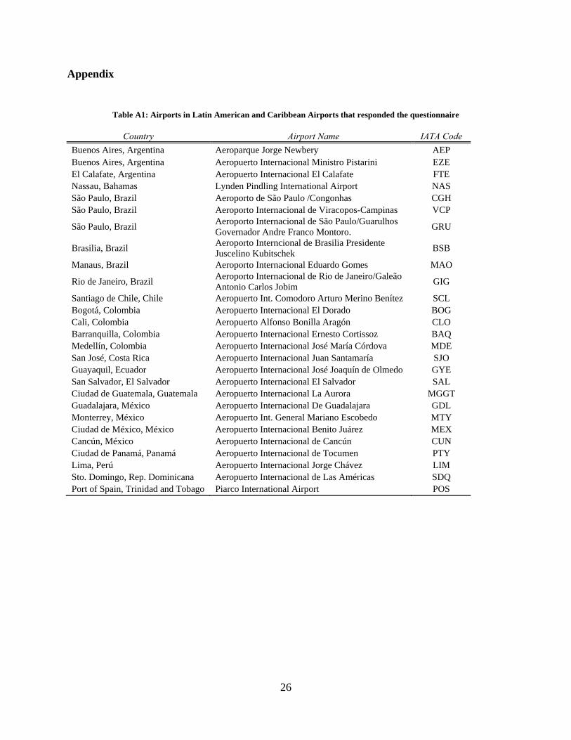
The main objective of this paper is to fill this gap in the literature. We are able to do so using data collected from a questionnaire that was sent, as part of a World Bank study on airports, to the major airport operators in LAC (see Table A1 in the Appendix for a list of airports that responded to the questionnaire). It should be noted that the sample assembled for this study is representative of the air transport sector in the LAC region. Indeed, the airports included in the sample account for more than 80% of total passengers and aircraft movements in the region and for 70% of total air cargo.
The paper first computes a data envelopment analysis (DEA) activity frontier for commercial airports around the world, using the data collected through the questionnaire together with information from airports in Europe, North America and Asia-Pacific taken from the Airport Benchmarking Report elaborated by the Air Transport Research Society (ATRS). These estimations allow us to observe where LAC airports stand relative to the best practices in the sector. The method used also allows us to identify the peers of each airport in Latin America (i.e. airports around the world which are comparable to LAC airports and which operate on the efficiency frontier).
We then proceed to identify factors that drive the observed differences in technical efficiency in the airport sector. In order to do this we estimate a truncated regression model using the efficiency scores of the DEA activity frontier as the dependent variable, and as independent variables several factors that attempt to capture the institutional framework and socioeconomic environment in which airports operate as well as other airport specific characteristics.
Finally, the dataset we use in this paper also allows us to measure Total Factor Productivity Changes (TFPC) for LAC airports over the period 1995-2007. The methodology used to perform these estimations consists on the computation of a Malmquist quantity index of TFPC based on the non-parametric DEA approach.
3
The rest of the paper is organized as follows. Section 2 presents a brief review of the existing related literature. In Section 3 we present our estimations of a DEA activity frontier for commercial airports around the world and use these results to identify the peers of each of the airports in LAC. Section 4 studies the determinants of airport efficiency by estimating a truncated regression model. Section 5 presents Malmquist quantity indexes of TFPC for LAC airports over the period 1995-2007. Finally, Section 6 presents some concluding remarks.
2. Literature Review
Guillen and Lall (1997) pioneered the use of Data Envelopment Analysis techniques to study efficiency in the airport sector. Their paper uses data from 21 US airports for the period 1989-1993. Using this dataset they define airports as producing two different classes of services – terminal services and movements – and then proceed to compute two different DEA frontiers, one for each of these two services. Finally, using Tobit regressions, they estimate the effect that different variables (like whether or not an airport has rotational runways, preferential runway use or existence of airport operational constraints) have on the efficiency scores of each airport.
Following Guillen and Lall (1997), a literature flourished using DEA methods to study the technical efficiency of the airport sector. In what follows we do not attempt to provide a complete account of this literature. Instead, we review the set of existing papers that is the most relevant for our paper. For a more complete and comprehensive account we refer the reader to Pestana Barros and Dieke (2008) 2.
Using a Malmquist total factor productivity index and data envelopment analysis, Abbot and Wu (2002) investigate the efficiency and productivity of Australian airports during the 1990s. Their results show that Australian airports recorded strong growth in technological change and total factor productivity during this period. However, this growth was based almost exclusively on a shift of the production frontier, with growth in technical and scale efficiency lagging behind.
Pestana, Barros, and Dieke (2008) compute a single DEA frontier for Italian airports using data from the period 2001-2003. However, instead of using a Tobit regression to find determinants of airport efficiency as in Gillen and Lall (1997), following the suggestions made by Simar and Wilson (2007), they estimate a truncated regression. Among many other results, Pestana, Barros, and Dieke (2008) find that Hub airports tend to be more efficient and that privately operated airports also tend to have higher efficiency scores than their publicly operated counterparts. Following Pestana, Barros, and Dieke (2008) and Simar and Wilson (2007), in this paper we also rely on truncated regressions to study the determinants of the observed differences in airport efficiency.
It is worth highlighting that there are a few papers that study the efficiency of airports in Latin America. For example, Flor and de la Torre (2008) use DEA methods to analyze efficiency and total factor productivity of airports in Peru. Similarly, Fernandes and Pacheco (2002) employ DEA methods to compute a production frontier using data for Brazilian airports and Gomez
2 Some other examples not mentioned in the main text are Gillen and Lall (2001), Murillo-Melchor (1999) and Fung et al (2008).
4
Lobo and Gonzalez (2008) also employ DEA to compare only one airport in LAC (Benito Merino airport in Santiago de Chile) with a set of airports in other regions. However, these papers focus on the efficiency of the airport sector in one single Latin American country. Indeed, to the best extent of our knowledge, this paper is the first that computes a global efficient frontier for the airport sector including data from a representative set of Latin American countries. In contrast to previous studies, this paper identifies how far away Latin American airports stand from the best practice worldwide.
Given the trend towards the introduction of private sector participation in the airport sector, one of the variables we are interested in testing is the effect that ownership has on airport efficiency. There are other papers that study this issue. For example, using DEA methods Parker (1999) analyses the effect that privatization had on the efficiency level of British airports and finds that privatization had no noticeable impact on technical efficiency. Based on panel data for the major airports in Asia-Pacific, Europe and North America for the years 2001-2003, Oum, Adler and Yu (2006) study the effect that the type of ownership has on productive efficiency and profitability. Their results suggest that airports with government majority ownership and those owned by multi-level government are significantly less efficient than airports operating under private majority ownership.
Lastly, it should be noted that DEA is not the only methodology available that can be used to study the efficiency of the airport sector.3 Indeed, some authors have studied productivity in this sector through methods different than DEA. For instance, Hooper and Hensher (1997) use index number methods to study the evolution of total factor productivity of Australian airports for the period 1988-1992. Oum, Yan and Yu (2008) study the effects of ownership types on airports' cost efficiency by applying stochastic frontier analysis to a panel data of the world's major airports. Pestana Barros (2008) also uses stochastic frontier analysis to study the technical efficiency of airports in the UK. Finally, analyzing the efficiency of European airports, Pels, Nijkamp and Rietveld (2001) compare the results they get from DEA methods to the results obtained using stochastic frontier analysis. Their analysis shows that the stochastic frontier model they consider reproduces the DEA results in quite a reasonable way.
3. Computing a Technical Efficiency Frontier for Airports around the World
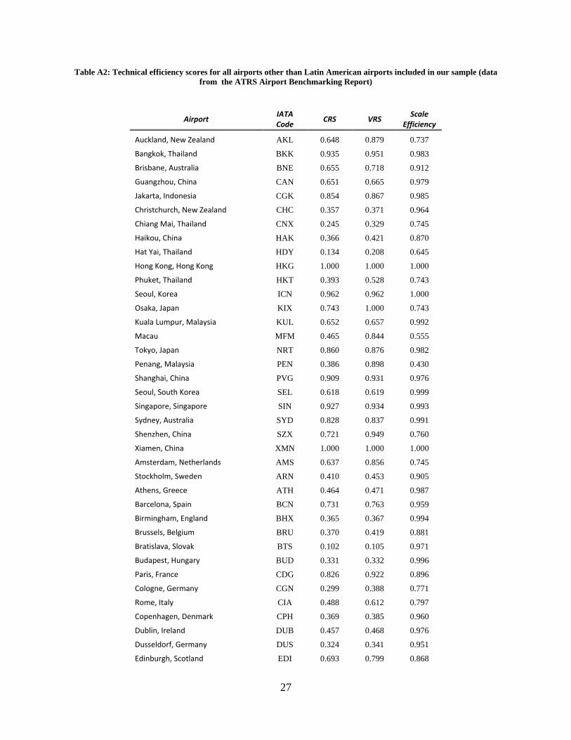
In this section we compute a DEA activity frontier for commercial airports around the world. We use data for the years 2005 and 2006 from 22 LAC airports, in addition to 23 airports from Asia-Pacific, 40 from Europe and 63 from Canada and the US (see Tables A1 and A2 in the Appendix for details of airports included in the sample and the results for non Latin American airports).
DEA is a deterministic non parametric approach used to build a benchmark, best practice frontier, based on available information. The method was first developed by Farrel (1957) and later consolidated by Charnes et al (1978). One of the main advantages of this approach is that it takes into account the multi-output multi-input dimensionality of production. Another advantage is that computations are based exclusively on measures of physical outputs and inputs, without
3 For a complete and updated presentation of frontier analysis methods proposed in the literature, see Coelli et al. (2005) and Fried, Lovell and Schmit (2008).
5
the need of using prices, which are neither available nor are comparable, mainly at the international level.
Two models are computed under the competing assumptions of constant returns to scale (CRS) and variable returns to scale (VRS). This allows us to compute scale efficiencies and to identify for each airport the returns to scale region - increasing, constant or decreasing - in which it operates. We assume that airports have as production target the maximization of outputs for a given input combination; therefore, we use an output oriented framework.
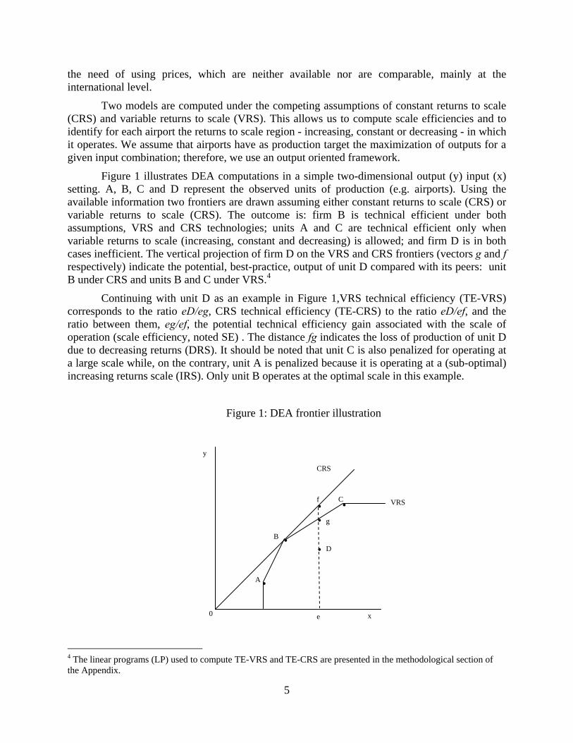
Figure 1 illustrates DEA computations in a simple two-dimensional output (y) input (x) setting. A, B, C and D represent the observed units of production (e.g. airports). Using the available information two frontiers are drawn assuming either constant returns to scale (CRS) or variable returns to scale (CRS). The outcome is: firm B is technical efficient under both assumptions, VRS and CRS technologies; units A and C are technical efficient only when variable returns to scale (increasing, constant and decreasing) is allowed; and firm D is in both cases inefficient. The vertical projection of firm D on the VRS and CRS frontiers (vectors g and f respectively) indicate the potential, best-practice, output of unit D compared with its peers: unit B under CRS and units B and C under VRS.4
Continuing with unit D as an example in Figure 1,VRS technical efficiency (TE-VRS) corresponds to the ratio eD/eg, CRS technical efficiency (TE-CRS) to the ratio eD/ef, and the ratio between them, eg/ef, the potential technical efficiency gain associated with the scale of operation (scale efficiency, noted SE) . The distance fg indicates the loss of production of unit D due to decreasing returns (DRS). It should be noted that unit C is also penalized for operating at a large scale while, on the contrary, unit A is penalized because it is operating at a (sub-optimal) increasing returns scale (IRS). Only unit B operates at the optimal scale in this example.
Figure 1: DEA frontier illustration
4 The linear programs (LP) used to compute TE-VRS and TE-CRS are presented in the methodological section of the Appendix.
y
x
0
A
D
C
B
f
e
CRS
VRS
g
6
Frontier models like DEA require the specification of inputs and outputs used in the industry under study. There have been considerable differences in the literature of airport efficiency estimation at the time of defining inputs and outputs. On the output side the more complete and often used model specification includes three output dimensions: passenger, freight and aircraft movements. On the inputs side there is fewer consensuses in the literature, mainly due to data availability problems. In any case, most studies include a bundle of variables representing labor and capital inputs. The most frequently used variables are the number of employees as proxy for labor input and capital proxies such as the number or size of runways, terminal size and the number of boarding bridges. When comparable accounting data is available, inputs are represented by operating costs and the monetary value of the capital stock.
In our case, and given the data at our disposal, we chose to specify a three-input three-output production function. The outputs that we use are (i) number of passengers, (ii) tons of freight and (iii) number of aircraft movements while the inputs are: (i) number of employees, (ii) number of runways and (iii) number of boarding bridges.
The dataset is well balanced for the 22 LAC airports but unbalanced for the other regions of the world, particularly for European airports. For this reason, we chose to pool and computed a single DEA frontier for the period 2005-2006.
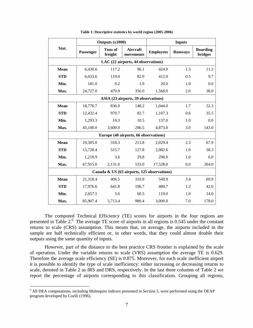
Table 1 presents descriptive statistics on outputs and inputs by region. LAC airports are on average smaller than those from the other regions in terms of all three outputs: passenger, tons and aircraft movements. However, in spite of these differences in the scale of production, on average LAC airports employ nearly as much staff as Canadian and US airports5. At the same time, in terms of capital investments, the number of runways and boarding bridges is several times lower in LAC airports than in Canadian and US airports.
5 The observed difference in employees does not directly imply there is over employment in LAC airports. The difference could be the result of different approaches to outsourcing airport services.
7
Table 1: Descriptive statistics by world region (2005-2006)
Stat.
Outputs (x1000) Inputs
Passenger Tons of freight
Aircraft movements
Employees Runways Boarding bridges
LAC (22 airports, 44 observations)
Mean 6,430.6 117.2 96.1 424.0 1.5 11.3
STD 6,033.6 119.0 82.9 412.0 0.5 9.7
Min. 181.0 0.2 1.9 20.0 1.0 0.0
Max. 24,727.0 470.9 356.0 1,568.0 2.0 38.0
ASIA (23 airports, 39 observations)
Mean 18,776.7 836.0 148.2 1,044.0 1.7 52.3
STD 12,432.4 970.7 82.7 1,107.3 0.6 35.5
Min. 1,293.3 10.3 10.5 137.0 1.0 0.0
Max. 45,100.0 3,600.0 286.5 4,873.0 3.0 143.0
Europe (40 airports, 66 observations)
Mean 19,305.0 318.3 211.8 2,029.4 2.3 67.9
STD 15,728.4 515.7 127.8 2,982.6 1.0 58.3
Min. 1,218.9 3.6 29.8 298.0 1.0 6.0
Max. 67,915.0 2,131.0 533.0 17,528.0 6.0 264.0
Canada & US (63 airports, 125 observations)
Mean 21,318.4 406.5 310.9 549.9 3.4 69.9
STD 17,976.6 641.8 196.7 480.7 1.2 42.6
Min. 2,657.1 3.6 60.5 119.0 1.0 14.0
Max. 85,907.4 3,713.4 980.4 3,000.0 7.0 178.0
The computed Technical Efficiency (TE) scores for airports in the four regions are presented in Table 2.6 The average TE score of airports in all regions is 0.545 under the constant returns to scale (CRS) assumption. This means that, on average, the airports included in the sample are half technically efficient or, in other words, that they could almost double their outputs using the same quantity of inputs.
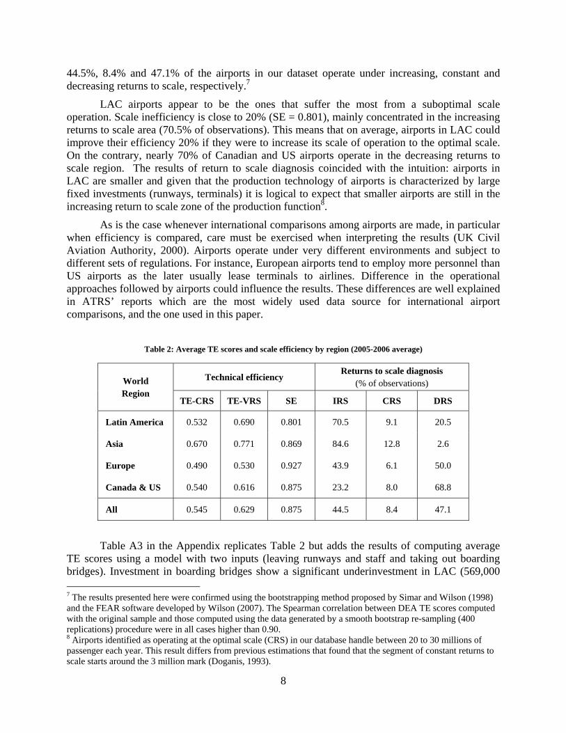
However, part of the distance to the best practice CRS frontier is explained by the scale of operation. Under the variable returns to scale (VRS) assumption the average TE is 0.629. Therefore the average scale efficiency (SE) is 0.875. Moreover, for each scale inefficient airport it is possible to identify the type of scale inefficiency: either increasing or decreasing returns to scale, denoted in Table 2 as IRS and DRS, respectively. In the last three columns of Table 2 we report the percentage of airports corresponding to this classification. Grouping all regions,
6 All DEA computations, including Malmquist indexes presented in Section 5, were performed using the DEAP program developed by Coelli (1996).
8
44.5%, 8.4% and 47.1% of the airports in our dataset operate under increasing, constant and decreasing returns to scale, respectively.7
LAC airports appear to be the ones that suffer the most from a suboptimal scale operation. Scale inefficiency is close to 20% (SE = 0.801), mainly concentrated in the increasing returns to scale area (70.5% of observations). This means that on average, airports in LAC could improve their efficiency 20% if they were to increase its scale of operation to the optimal scale. On the contrary, nearly 70% of Canadian and US airports operate in the decreasing returns to scale region. The results of return to scale diagnosis coincided with the intuition: airports in LAC are smaller and given that the production technology of airports is characterized by large fixed investments (runways, terminals) it is logical to expect that smaller airports are still in the increasing return to scale zone of the production function8.
As is the case whenever international comparisons among airports are made, in particular when efficiency is compared, care must be exercised when interpreting the results (UK Civil Aviation Authority, 2000). Airports operate under very different environments and subject to different sets of regulations. For instance, European airports tend to employ more personnel than US airports as the later usually lease terminals to airlines. Difference in the operational approaches followed by airports could influence the results. These differences are well explained in ATRS’ reports which are the most widely used data source for international airport comparisons, and the one used in this paper.
Table 2: Average TE scores and scale efficiency by region (2005-2006 average)
World Region
Technical efficiency Returns to scale diagnosis
(% of observations)
TE-CRS TE-VRS SE IRS CRS DRS
Latin America 0.532 0.690 0.801 70.5 9.1 20.5
Asia 0.670 0.771 0.869 84.6 12.8 2.6
Europe 0.490 0.530 0.927 43.9 6.1 50.0
Canada & US 0.540 0.616 0.875 23.2 8.0 68.8
All 0.545 0.629 0.875 44.5 8.4 47.1
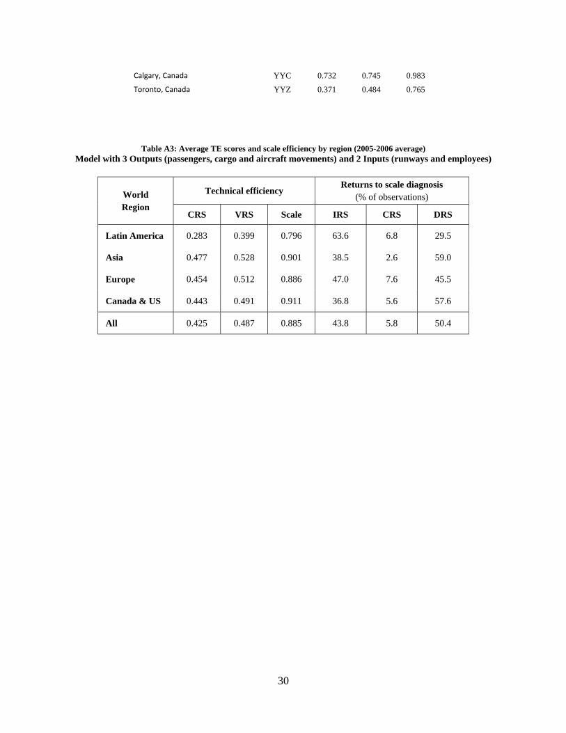
Table A3 in the Appendix replicates Table 2 but adds the results of computing average TE scores using a model with two inputs (leaving runways and staff and taking out boarding bridges). Investment in boarding bridges show a significant underinvestment in LAC (569,000 7 The results presented here were confirmed using the bootstrapping method proposed by Simar and Wilson (1998) and the FEAR software developed by Wilson (2007). The Spearman correlation between DEA TE scores computed with the original sample and those computed using the data generated by a smooth bootstrap re-sampling (400 replications) procedure were in all cases higher than 0.90. 8 Airports identified as operating at the optimal scale (CRS) in our database handle between 20 to 30 millions of passenger each year. This result differs from previous estimations that found that the segment of constant returns to scale starts around the 3 million mark (Doganis, 1993).
9
passengers per boarding bridge, compared with 359,000, 284,000 and 305,000 in Asia, Europe and North America respectively) and given that robust and comparable information on quality is not available, with the specification of inputs and outputs chosen in this paper, DEA tends to reward airports that underinvest in capital. When taking out boarding bridges the average TE score for LAC airports fall significantly relative to the average in other regions.
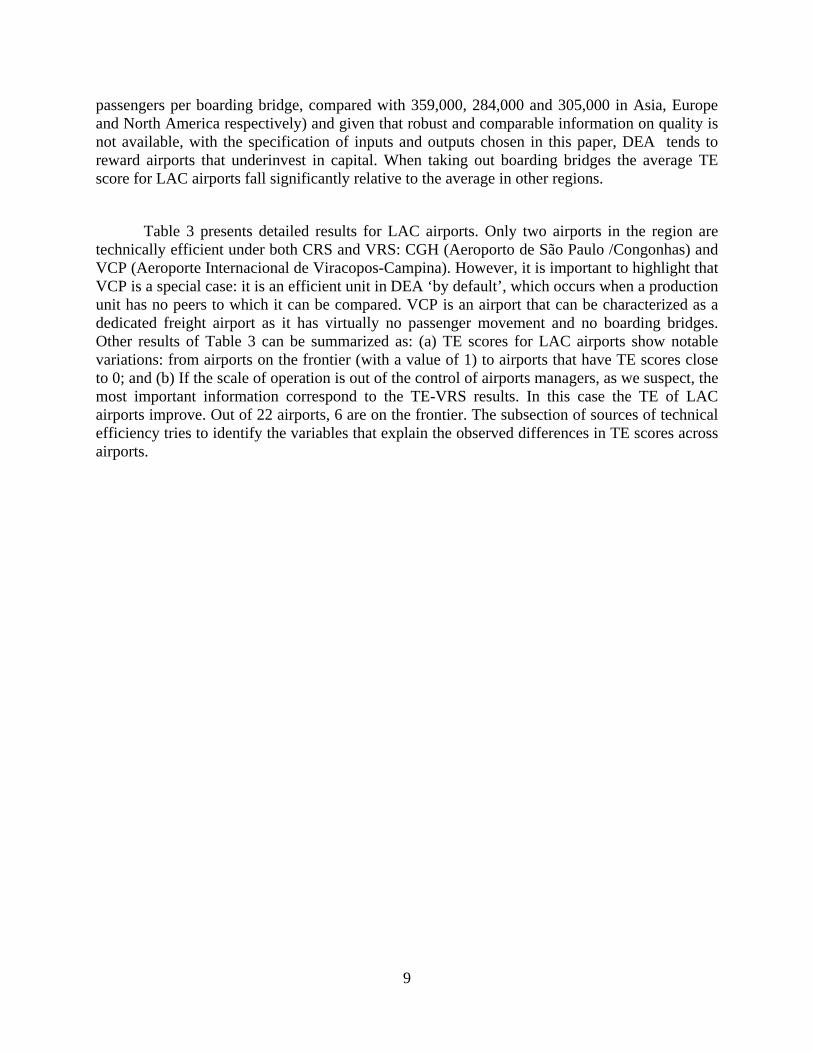
Table 3 presents detailed results for LAC airports. Only two airports in the region are technically efficient under both CRS and VRS: CGH (Aeroporto de São Paulo /Congonhas) and VCP (Aeroporte Internacional de Viracopos-Campina). However, it is important to highlight that VCP is a special case: it is an efficient unit in DEA ‘by default’, which occurs when a production unit has no peers to which it can be compared. VCP is an airport that can be characterized as a dedicated freight airport as it has virtually no passenger movement and no boarding bridges. Other results of Table 3 can be summarized as: (a) TE scores for LAC airports show notable variations: from airports on the frontier (with a value of 1) to airports that have TE scores close to 0; and (b) If the scale of operation is out of the control of airports managers, as we suspect, the most important information correspond to the TE-VRS results. In this case the TE of LAC airports improve. Out of 22 airports, 6 are on the frontier. The subsection of sources of technical efficiency tries to identify the variables that explain the observed differences in TE scores across airports.
10
Table 3: Technical efficiency and scale efficiency scores (2005-2006 average)
Country Airport TE-CRS TE-VRS SE
Argentina
AEP 0.612 0.998 0.614
EZE 0.414 0.417 0.993
FTE 0.115 1.000 0.115
Brazil
BSB 0.498 0.536 0.931
CGH 1.000 1.000 1.000
GIG 0.318 0.320 0.994
GRU 0.677 0.678 0.998
MAO 0.377 0.692 0.544
VCP 1.000 1.000 1.000
Chile SCL 0.786 1.000 0.786
Colombia BAQ 0.329 0.524 0.628
CLO 0.496 0.734 0.676
Costa Rica SJO 0.594 0.983 0.605
Ecuador GYE 0.472 0.646 0.739
El Salvador SAL 0.114 0.127 0.900
Mexico
CUN 0.860 1.000 0.860
GDL 0.643 0.649 0.991
MEX 0.961 0.963 0.998
MTY 0.403 0.410 0.982
Panama PTY 0.164 0.178 0.926
Peru LIM 0.621 0.961 0.646
Dominican Rep. SDQ 0.260 0.372 0.699
ALL 0.532 0.690 0.801
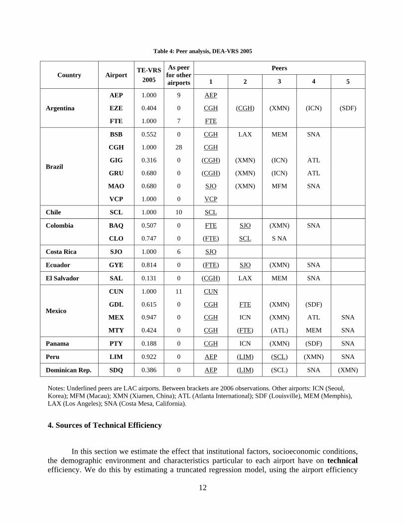
The use of DEA allows the identification of peers for each airport, which are the set of efficient airports that make up the relevant frontier for a given airport. Table 4 presents the peers for LAC airports in 2005 under the VRS model. Observations for peers corresponding to 2006 are in brackets and airport peers from the LAC region appear underlined. It should be noted that, by construction, technically efficient airports do not have other airport as peers. Technical inefficient airports have, on the contrary, a benchmark composed by other units. Given the 3-output 3-inputs dimensionality of the production setting, the maximum number of peers is 6 but an airport can have less than 6 peers.
11
It is important to remark that some LAC airports are peers for other airports. Not only do they serve as peers (benchmark) for other airports in the LAC region but also for other airports around the world. This is the case mainly of CGH, which is a reference for 28 observations (2005 and 2006 airport observations taken together). Other airports playing the same role of peers are AEP (Aeroparque Jorge Newbery, Buenos Aires), SCL (Comodoro Merino Benítez, Santiago de Chile), CUN (Cancún) and, to a less extent, FTE (Aeropuerto Internacional de El Calafate) and SJO (Aeropuerto Internacional Juan Santamaria, San José, Costa Rica). An interesting result is that all LAC airports in our sample, with the exception of MAO (Aeroporto Internacional Eduardo Gomes, Manaus), have as peers at least one Latin American airport. Eight airports from outside the LAC region act as peers for LAC airports: XMN (Xaimen), ICN (Seoul), SDF (Louisville), LAX (Los Angeles), MEM (Memphis), SNA (Costa Mesa, California), ATL (Atlanta) and MFM (Macau).
For illustration purposes, let us look in more detail at one observation, the case of BSB (Aeroporto Internacional Juscelino Kubitschek, Brasilia). For this airport we computed a TE-VRS score of 0.552, which corresponds to a 45% output inefficiency diagnosis. The airports identified as peers for BSB are CGH and three US airports: MEM (Memphis), LAX (Los Angeles) and SNA (Costa Mesa, California). If we simply compare BSB against CGH, its only LAC peer, and look at some of their main output-input features (for the year 2005), we get a confirmation of the DEA result. On the output side BSB handles 9.4 million passengers per year, against the 17.1 million passengers of CGH. Similarly, BSB had 171.6 thousand aircraft movements in 2005, against 282.6 thousand aircraft movements in CGH. Finally, on the input side we see that BSB had 365 employees and 13 boarding bridges, while CGH had 225 employees and 8 boarding bridges.
12
Table 4: Peer analysis, DEA-VRS 2005
Country Airport TE-VRS
2005
As peer for other airports
Peers
1 2 3 4 5
Argentina
AEP 1.000 9 AEP
EZE 0.404 0 CGH (CGH) (XMN) (ICN) (SDF)
FTE 1.000 7 FTE
Brazil
BSB 0.552 0 CGH LAX MEM SNA
CGH 1.000 28 CGH
GIG 0.316 0 (CGH) (XMN) (ICN) ATL
GRU 0.680 0 (CGH) (XMN) (ICN) ATL
MAO 0.680 0 SJO (XMN) MFM SNA
VCP 1.000 0 VCP
Chile SCL 1.000 10 SCL
Colombia BAQ 0.507 0 FTE SJO (XMN) SNA
CLO 0.747 0 (FTE) SCL S NA
Costa Rica SJO 1.000 6 SJO
Ecuador GYE 0.814 0 (FTE) SJO (XMN) SNA
El Salvador SAL 0.131 0 (CGH) LAX MEM SNA
Mexico
CUN 1.000 11 CUN
GDL 0.615 0 CGH FTE (XMN) (SDF)
MEX 0.947 0 CGH ICN (XMN) ATL SNA
MTY 0.424 0 CGH (FTE) (ATL) MEM SNA
Panama PTY 0.188 0 CGH ICN (XMN) (SDF) SNA
Peru LIM 0.922 0 AEP (LIM) (SCL) (XMN) SNA
Dominican Rep. SDQ 0.386 0 AEP (LIM) (SCL) SNA (XMN)
Notes: Underlined peers are LAC airports. Between brackets are 2006 observations. Other airports: ICN (Seoul, Korea); MFM (Macau); XMN (Xiamen, China); ATL (Atlanta International); SDF (Louisville), MEM (Memphis), LAX (Los Angeles); SNA (Costa Mesa, California).
4. Sources of Technical Efficiency
In this section we estimate the effect that institutional factors, socioeconomic conditions, the demographic environment and characteristics particular to each airport have on technical efficiency. We do this by estimating a truncated regression model, using the airport efficiency
13
scores of the previous section as dependent variables and these factors as explanatory variables. The choice of a truncated model is dictated by the nature of the technical efficiency measure (which is by definition truncated at 1.0) and by the findings of the recent academic literature (Simar and Wilson (2007)).9
Before presenting our results we stress that service quality is likely to be another potential factor behind the observed differences in airport efficiency. It is likely that, other things equal, airports operating with a large staff and/or a large number of boarding bridges provide better service quality to passengers. Unfortunately, survey data on users’ satisfaction is not yet available at an international scale for us to be able to include quality indicators in our regression analysis.
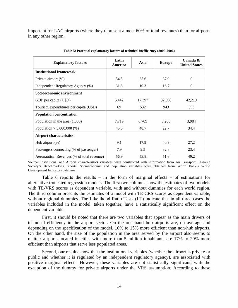
Table 5 presents average values by region for the candidate variables to account for observed differences in technical efficiency. Starting with the institutional setting, Table 5 shows that on average LAC airports operate under a more liberalized framework. Indeed, more than half of LAC airports (54.5%) in our sample operate as private concessions, and 31.8% are regulated by an independent regulatory agency. In contrast, only 25.6% of Asian airports and 37.9% of European airports are under private management, while 10.3% and 16.7% of Asian and European airports respectively are regulated by an independent regulatory agency. Finally, all airports in Canada and the United States are operated by state-owned enterprises, and regulatory agencies in these two countries still depend directly from a political authority (a ministry).
Another potential factor that could have a role in the explanation of airport performance is the socioeconomic environment in which they operate. We incorporate this effect with two indicators: GDP per capita (measured in current dollars) and tourism expenditures (also measured in current dollars). However, it is worth stressing that these variables are only available at the country level and don’t correspond necessarily to the area of influence of the airports.10
The demographic environment is represented by the concentration of population in the area served by the airport. On average, LAC airports appear to serve very large urban agglomerations, like their Asian counterparts. Compared to European and North-American airports, which are on average located in cities with 3 to 4 million inhabitants, LAC airports are on average located in cities with 8 million people. In the regression analysis this information will be incorporated with a binary (dummy) variable that takes a value 1 for airports located in cities with more than 5 million people and 0 otherwise11.
Finally, we introduce a set of variables that represent characteristics that are particular to each airport. One of them is their specialization as a hub, represented by the percentage of connecting passengers. LAC airports have the lowest percentage of connecting passengers (and also have the lowest percentage of hubs), followed by Asian airports. The highest percentage is observed among European airports, where nearly one-third of passengers are connecting. Another variable that is particular to each airport is the share of aeronautical revenues in total revenues. In Table 5 below we see that aeronautical revenues are on average rather more
9 We estimate truncated regressions using the “truncreg” procedure of SATA 9.0. 10 Given that our dataset contains several airports in the United States and given the availability of data, for these airports we used GDP per capita of the state in which each airport is located instead of GDP per capita for the country as a whole. 11 The value of 5 million corresponds to the mean of the population of the cities where airports are located.
14
important for LAC airports (where they represent almost 60% of total revenues) than for airports in any other region.
Table 5: Potential explanatory factors of technical inefficiency (2005-2006)
Explanatory factors Latin
America Asia Europe
Canada & United States
Institutional framework
Private airport (%) 54.5 25.6 37.9 0
Independent Regulatory Agency (%) 31.8 10.3 16.7 0
Socioeconomic environment
GDP per capita (U$D) 5,442 17,397 32,598 42,219
Tourism expenditures per capita (U$D) 69 532 943 393
Population concentration
Population in the area (1,000) 7,719 6,709 3,200 3,984
Population > 5,000,000 (%) 45.5 48.7 22.7 34.4
Airport characteristics
Hub airport (%) 9.1 17.9 40.9 27.2
Passengers connecting (% of passenger) 7.9 9.5 32.8 23.4
Aeronautical Revenues (% of total revenue) 56.9 53.8 51.6 49.2
Source: Institutional and Airport characteristics variables were constructed with information from Air Transport Research Society’s Benchmarking reports. Socioeconomic and population variables were obtained from World Bank’s World Development Indicators database.
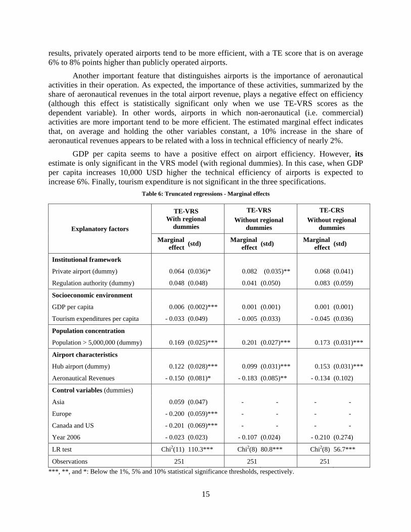
Table 6 reports the results – in the form of marginal effects – of estimations for alternative truncated regression models. The first two columns show the estimates of two models with TE-VRS scores as dependent variable, with and without dummies for each world region. The third column presents the estimates of a model with TE-CRS scores as dependent variable, without regional dummies. The Likelihood Ratio Tests (LT) indicate that in all three cases the variables included in the model, taken together, have a statistically significant effect on the dependent variable.
First, it should be noted that there are two variables that appear as the main drivers of technical efficiency in the airport sector. On the one hand hub airports are, on average and depending on the specification of the model, 10% to 15% more efficient than non-hub airports. On the other hand, the size of the population in the area served by the airport also seems to matter: airports located in cities with more than 5 million inhabitants are 17% to 20% more efficient than airports that serve less populated areas.
Second, our results show that the institutional variables (whether the airport is private or public and whether it is regulated by an independent regulatory agency), are associated with positive marginal effects. However, these variables are not statistically significant, with the exception of the dummy for private airports under the VRS assumption. According to these
15
results, privately operated airports tend to be more efficient, with a TE score that is on average 6% to 8% points higher than publicly operated airports.
Another important feature that distinguishes airports is the importance of aeronautical activities in their operation. As expected, the importance of these activities, summarized by the share of aeronautical revenues in the total airport revenue, plays a negative effect on efficiency (although this effect is statistically significant only when we use TE-VRS scores as the dependent variable). In other words, airports in which non-aeronautical (i.e. commercial) activities are more important tend to be more efficient. The estimated marginal effect indicates that, on average and holding the other variables constant, a 10% increase in the share of aeronautical revenues appears to be related with a loss in technical efficiency of nearly 2%.
GDP per capita seems to have a positive effect on airport efficiency. However, its estimate is only significant in the VRS model (with regional dummies). In this case, when GDP per capita increases 10,000 USD higher the technical efficiency of airports is expected to increase 6%. Finally, tourism expenditure is not significant in the three specifications.
Table 6: Truncated regressions - Marginal effects
Explanatory factors
TE-VRS With regional
dummies
TE-VRS
Without regional dummies
TE-CRS
Without regional dummies
Marginal effect
(std) Marginal
effect (std)
Marginal effect
(std)
Institutional framework
Private airport (dummy) 0.064 (0.036)* 0.082 (0.035)** 0.068 (0.041)
Regulation authority (dummy) 0.048 (0.048) 0.041 (0.050) 0.083 (0.059)
Socioeconomic environment
GDP per capita 0.006 (0.002)*** 0.001 (0.001) 0.001 (0.001)
Tourism expenditures per capita - 0.033 (0.049) - 0.005 (0.033) - 0.045 (0.036)
Population concentration
Population > 5,000,000 (dummy) 0.169 (0.025)*** 0.201 (0.027)*** 0.173 (0.031)***
Airport characteristics
Hub airport (dummy) 0.122 (0.028)*** 0.099 (0.031)*** 0.153 (0.031)***
Aeronautical Revenues - 0.150 (0.081)* - 0.183 (0.085)** - 0.134 (0.102)
Control variables (dummies)
Asia 0.059 (0.047) - - - -
Europe - 0.200 (0.059)*** - - - -
Canada and US - 0.201 (0.069)*** - - - -
Year 2006 - 0.023 (0.023) - 0.107 (0.024) - 0.210 (0.274)
LR test Chi2(11) 110.3*** Chi2(8) 80.8*** Chi2(8) 56.7***
Observations 251 251 251
***, **, and *: Below the 1%, 5% and 10% statistical significance thresholds, respectively.
16
5. Measuring Productivity Change of LAC Airports
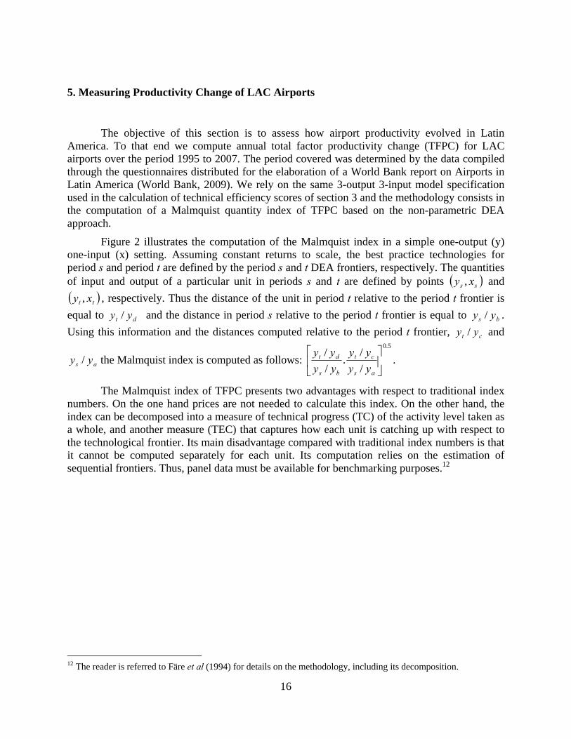
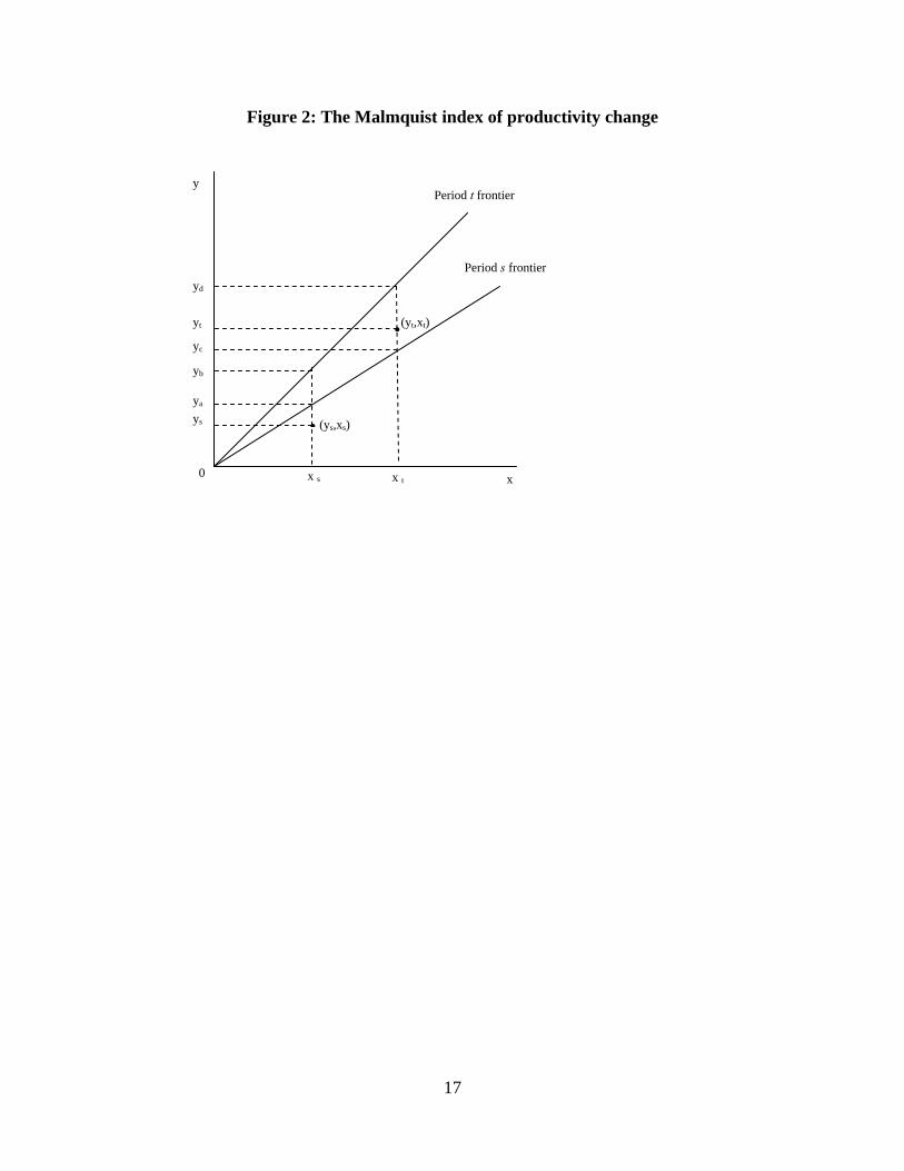
The objective of this section is to assess how airport productivity evolved in Latin America. To that end we compute annual total factor productivity change (TFPC) for LAC airports over the period 1995 to 2007. The period covered was determined by the data compiled through the questionnaires distributed for the elaboration of a World Bank report on Airports in Latin America (World Bank, 2009). We rely on the same 3-output 3-input model specification used in the calculation of technical efficiency scores of section 3 and the methodology consists in the computation of a Malmquist quantity index of TFPC based on the non-parametric DEA approach.
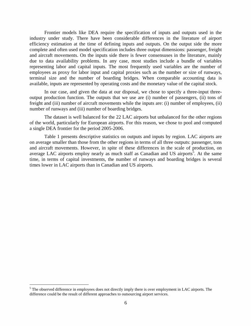
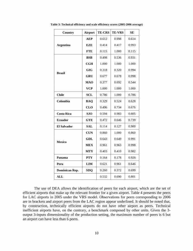
Figure 2 illustrates the computation of the Malmquist index in a simple one-output (y) one-input (x) setting. Assuming constant returns to scale, the best practice technologies for period s and period t are defined by the period s and t DEA frontiers, respectively. The quantities of input and output of a particular unit in periods s and t are defined by points ss xy , and
tt xy , , respectively. Thus the distance of the unit in period t relative to the period t frontier is
equal to dt yy / and the distance in period s relative to the period t frontier is equal to bs yy / .
Using this information and the distances computed relative to the period t frontier, ct yy / and
as yy / the Malmquist index is computed as follows: 5.0
/
/.
/
/
as
ct
bs
dt
yy
yy
yy
yy.
The Malmquist index of TFPC presents two advantages with respect to traditional index numbers. On the one hand prices are not needed to calculate this index. On the other hand, the index can be decomposed into a measure of technical progress (TC) of the activity level taken as a whole, and another measure (TEC) that captures how each unit is catching up with respect to the technological frontier. Its main disadvantage compared with traditional index numbers is that it cannot be computed separately for each unit. Its computation relies on the estimation of sequential frontiers. Thus, panel data must be available for benchmarking purposes.12
12 The reader is referred to Färe et al (1994) for details on the methodology, including its decomposition.
17
Figure 2: The Malmquist index of productivity change
y
x
0 x t
Period s frontier
Period t frontier
x s
yt
ys (ys,xs)
(yt,xt)
yc yb
yd
ya
18
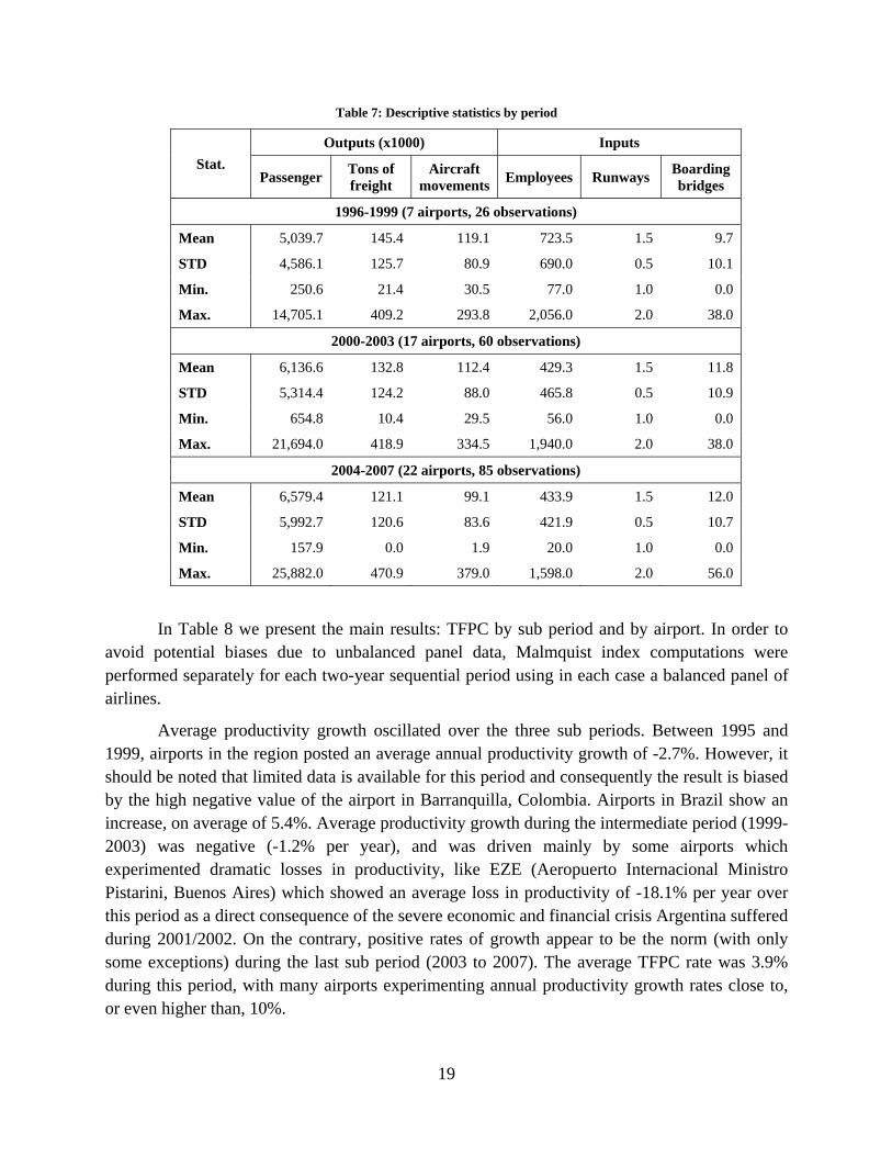
Table 7 presents descriptive statistics for the three sub periods in which we decomposed the sample: 1995-1999, 2000-2003 and 2004-2007. For each of these three sub periods the number of airports in our sample varies noticeably, from 7 to 22.13 As a consequence, the benchmark used for TFPC computations varies as well.14
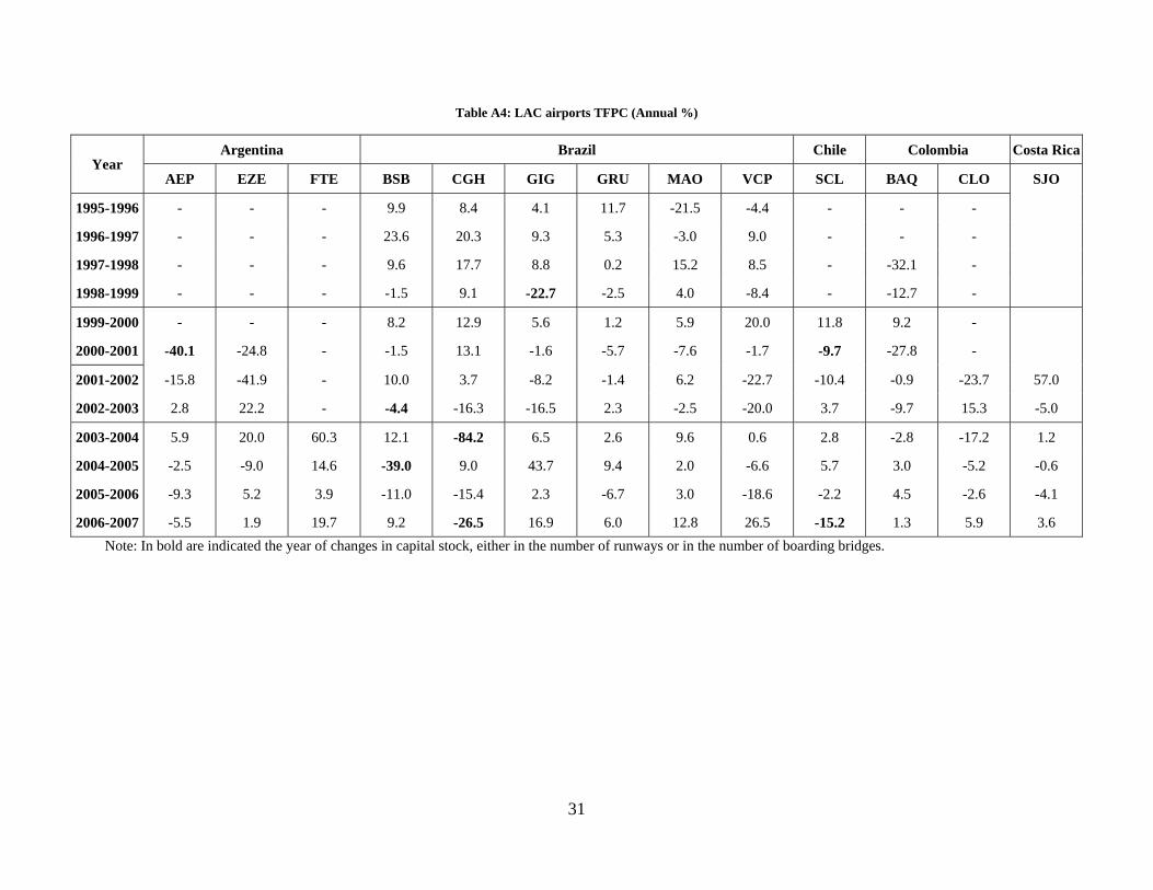
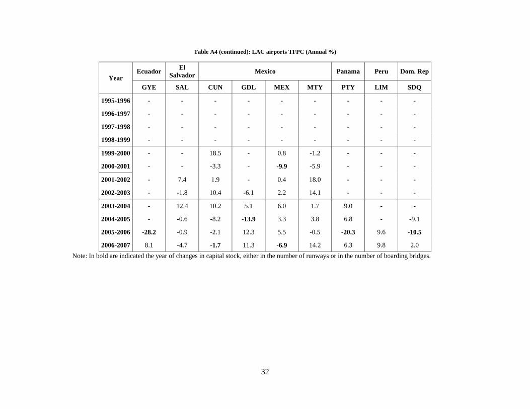
The average TFPC values reported in Table 8 exclude 14 over 154 observations. These observations correspond to airports which introduced major changes in their capital stock in a particular year (given by increases in either the number of runways or boarding bridges). Given that these types of investments are lumpy by nature and that their introduction is followed by an initial period of underutilization, they tend to have a big negative impact on measures of productivity change. Table A4 in the Appendix reports the results for all airports and years. Those cases corresponding to changes in the stock of either the number of runways or boarding bridges are in bold. As expected, the TFPC index corresponding to these observations are highly negative.
13 The only criterion used to split the data was to obtain 3 sub periods with equivalent number of years. The sample covers a large range of airports sizes. Measuring size by the number of passengers per year the sample ranges from 158,000 to 25,800,000 passengers. Zero values are reported for some variables. On the output side, this is the case for freight transportation for at least one airport. And on the input side, at least one airport is not equipped with boarding bridges, still in the year 2007. 14 Due to the unbalanced nature of our dataset we did not decomposed the TFPC results presented in Table 8.
19
Table 7: Descriptive statistics by period
Stat.
Outputs (x1000) Inputs
Passenger Tons of freight
Aircraft movements
Employees Runways Boarding bridges
1996-1999 (7 airports, 26 observations)
Mean 5,039.7 145.4 119.1 723.5 1.5 9.7
STD 4,586.1 125.7 80.9 690.0 0.5 10.1
Min. 250.6 21.4 30.5 77.0 1.0 0.0
Max. 14,705.1 409.2 293.8 2,056.0 2.0 38.0
2000-2003 (17 airports, 60 observations)
Mean 6,136.6 132.8 112.4 429.3 1.5 11.8
STD 5,314.4 124.2 88.0 465.8 0.5 10.9
Min. 654.8 10.4 29.5 56.0 1.0 0.0
Max. 21,694.0 418.9 334.5 1,940.0 2.0 38.0
2004-2007 (22 airports, 85 observations)
Mean 6,579.4 121.1 99.1 433.9 1.5 12.0
STD 5,992.7 120.6 83.6 421.9 0.5 10.7
Min. 157.9 0.0 1.9 20.0 1.0 0.0
Max. 25,882.0 470.9 379.0 1,598.0 2.0 56.0
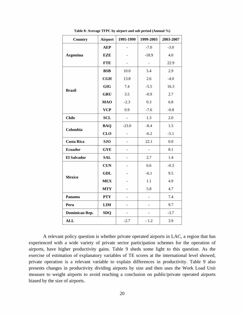
In Table 8 we present the main results: TFPC by sub period and by airport. In order to avoid potential biases due to unbalanced panel data, Malmquist index computations were performed separately for each two-year sequential period using in each case a balanced panel of airlines.
Average productivity growth oscillated over the three sub periods. Between 1995 and 1999, airports in the region posted an average annual productivity growth of -2.7%. However, it should be noted that limited data is available for this period and consequently the result is biased by the high negative value of the airport in Barranquilla, Colombia. Airports in Brazil show an increase, on average of 5.4%. Average productivity growth during the intermediate period (1999-2003) was negative (-1.2% per year), and was driven mainly by some airports which experimented dramatic losses in productivity, like EZE (Aeropuerto Internacional Ministro Pistarini, Buenos Aires) which showed an average loss in productivity of -18.1% per year over this period as a direct consequence of the severe economic and financial crisis Argentina suffered during 2001/2002. On the contrary, positive rates of growth appear to be the norm (with only some exceptions) during the last sub period (2003 to 2007). The average TFPC rate was 3.9% during this period, with many airports experimenting annual productivity growth rates close to, or even higher than, 10%.
20
Table 8: Average TFPC by airport and sub period (Annual %)
Country Airport 1995-1999 1999-2003 2003-2007
Argentina
AEP - -7.0 -3.0
EZE - -18.9 4.0
FTE - - 22.9
Brazil
BSB 10.0 5.4 2.9
CGH 13.8 2.6 -4.0
GIG 7.4 -5.5 16.3
GRU 3.5 -0.9 2.7
MAO -2.3 0.3 6.8
VCP 0.9 -7.6 -0.8
Chile SCL - 1.3 2.0
Colombia BAQ -23.0 -8.4 1.5
CLO - -6.2 -5.1
Costa Rica SJO - 22.1 0.0
Ecuador GYE - - 8.1
El Salvador SAL - 2.7 1.4
Mexico
CUN - 6.6 -0.3
GDL - -6.1 9.5
MEX - 1.1 4.9
MTY - 5.8 4.7
Panama PTY - - 7.4
Peru LIM - - 9.7
Dominican Rep. SDQ - - -3.7
ALL -2.7 - 1.2 3.9
A relevant policy question is whether private operated airports in LAC, a region that has experienced with a wide variety of private sector participation schemes for the operation of airports, have higher productivity gains. Table 9 sheds some light to this question. As the exercise of estimation of explanatory variables of TE scores at the international level showed, private operation is a relevant variable to explain differences in productivity. Table 9 also presents changes in productivity dividing airports by size and then uses the Work Load Unit measure to weight airports to avoid reaching a conclusion on public/private operated airports biased by the size of airports.
21
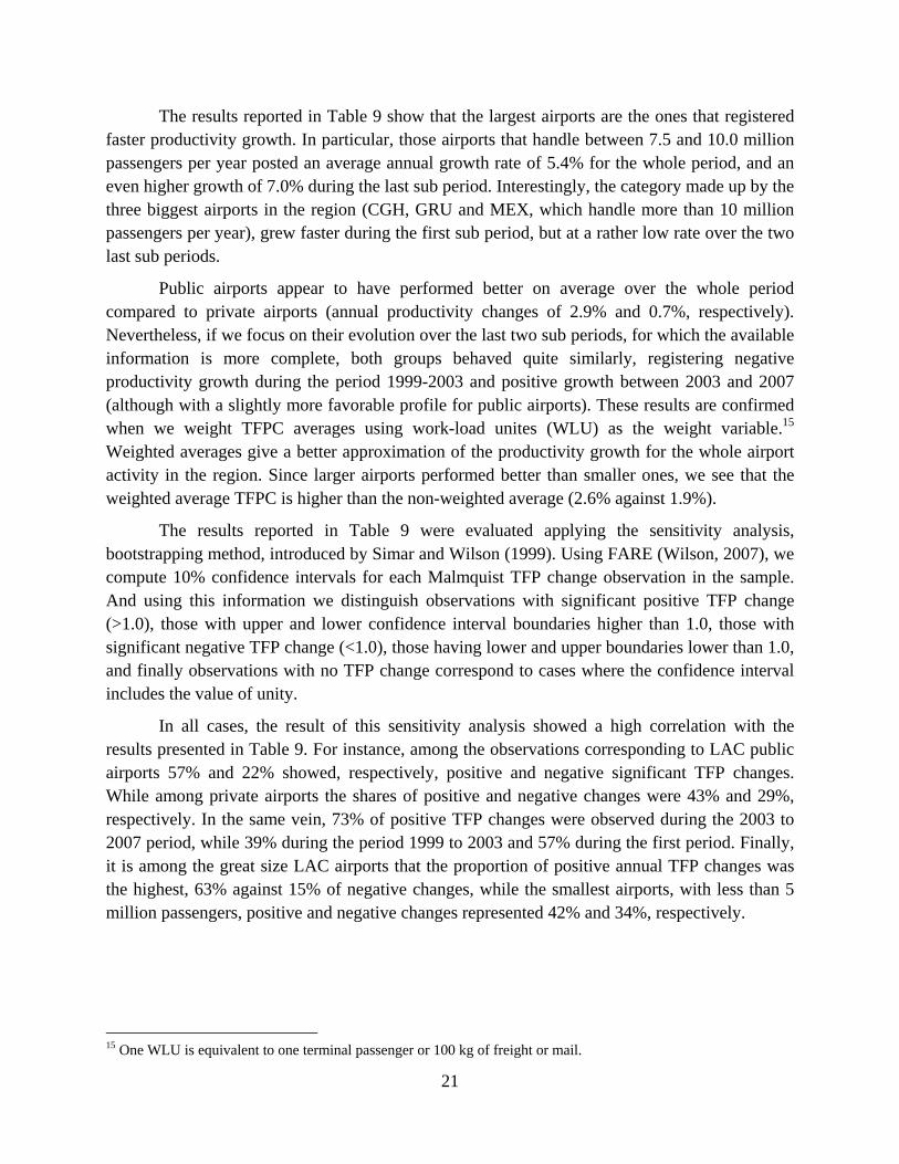
The results reported in Table 9 show that the largest airports are the ones that registered faster productivity growth. In particular, those airports that handle between 7.5 and 10.0 million passengers per year posted an average annual growth rate of 5.4% for the whole period, and an even higher growth of 7.0% during the last sub period. Interestingly, the category made up by the three biggest airports in the region (CGH, GRU and MEX, which handle more than 10 million passengers per year), grew faster during the first sub period, but at a rather low rate over the two last sub periods.
Public airports appear to have performed better on average over the whole period compared to private airports (annual productivity changes of 2.9% and 0.7%, respectively). Nevertheless, if we focus on their evolution over the last two sub periods, for which the available information is more complete, both groups behaved quite similarly, registering negative productivity growth during the period 1999-2003 and positive growth between 2003 and 2007 (although with a slightly more favorable profile for public airports). These results are confirmed when we weight TFPC averages using work-load unites (WLU) as the weight variable.15 Weighted averages give a better approximation of the productivity growth for the whole airport activity in the region. Since larger airports performed better than smaller ones, we see that the weighted average TFPC is higher than the non-weighted average (2.6% against 1.9%).
The results reported in Table 9 were evaluated applying the sensitivity analysis, bootstrapping method, introduced by Simar and Wilson (1999). Using FARE (Wilson, 2007), we compute 10% confidence intervals for each Malmquist TFP change observation in the sample. And using this information we distinguish observations with significant positive TFP change (>1.0), those with upper and lower confidence interval boundaries higher than 1.0, those with significant negative TFP change (<1.0), those having lower and upper boundaries lower than 1.0, and finally observations with no TFP change correspond to cases where the confidence interval includes the value of unity.
In all cases, the result of this sensitivity analysis showed a high correlation with the results presented in Table 9. For instance, among the observations corresponding to LAC public airports 57% and 22% showed, respectively, positive and negative significant TFP changes. While among private airports the shares of positive and negative changes were 43% and 29%, respectively. In the same vein, 73% of positive TFP changes were observed during the 2003 to 2007 period, while 39% during the period 1999 to 2003 and 57% during the first period. Finally, it is among the great size LAC airports that the proportion of positive annual TFP changes was the highest, 63% against 15% of negative changes, while the smallest airports, with less than 5 million passengers, positive and negative changes represented 42% and 34%, respectively.
15 One WLU is equivalent to one terminal passenger or 100 kg of freight or mail.
22
Table 9: Average TFPC by airport categories (Annual %)
Airport categories 1995-1999 1999-2003 2003-2007 ALL
Non-weighted
Size (106 passengers)
< 5.0 - 5.6 - 1.8 3.5 0.4
5.0 to 7.5 - - 4.3 3.7 0.5
7.5 to 10.0 8.9 1.7 7.0 5.4
> 10.0 8.5 0.9 1.8 3.4
Private-Public
Private - 23.0 - 1.6 3.4 0.7
Public 5.3 - 0.8 4.5 2.9
ALL 2.7 - 1.2 3.9 1.9
Weighted *
Private-Public
Private - 23.2 - 0.5 2.7 1.3
Public 6.1 0.2 4.4 3.2
ALL 5.5 0.0 3.7 2.6
* Weighted by WLU. Public airports: BSB, CGH, GIG, GRU, MAO and VCP (Brasil); SAL (El Salvador); MEX (México); and PTY (Panamá). Private airports: AEP, EZE, FTE (Argentina); SCL (Chile), BAQ and CLO (Colombia); SJO (Costa Rica); GYE (Ecuador); CUN GDL and MTY (México); and LIM (Perú). Airport size: < 5.0: BAQ, CLO, FTE, GYE, MAO, PTY, SAL, SDQ and SJO; 5.0-7.5: AEP, EZE, GDL, LIM, MTY and SCL; 7.5-10.0: BSB, CUN and GIG; > 10.0: CGH, GRU and MEX.
6. Conclusions
To the best extent of our knowledge, this paper is the first to conduct a comprehensive efficiency calculation of Latin American airports. Our results indicate that technical efficiency in Latin American airports shows notable variations: from airports on the frontier (with a value of 1) to airports that have technical efficiency scores close to 0. When variable returns to scale are assumed (which implies that the scale of operation is out of the control of airport managers, a sensible assumption) of the 22 LAC airports in the sample, 6 are on the frontier. However, when constant returns to scale are considered, only two airports are on the frontier.
On average, Latin American airports are less efficient than Asian and North American airports when constant returns to scale are assumed, but more efficient than European airports. However, when boarding bridges are excluded and not considered as a proxy for capital
23
investments, LAC airports are on average significantly less efficient than those in the other regions included in the study.
Using the DEA efficiency scores, we estimated a truncated regression model in order to find factors that might explain the observed differences in airport efficiency. As expected, the regression analysis shows that hub airports tend to be more efficient. Moreover, airports which are located in cities with more than 5 million inhabitants are also more efficient than airports located in smaller cities. The level of income (GDP) also seems to positively influence productive efficiency. Airports that rely more on revenue sources other than aeronautical tariffs also tend to be more efficient, a finding consistent with the recent literature (ATRS, 2008). Finally, airports which are privately operated tend to stand closer to the efficient frontier than their publicly operated counterparts, although this effect is not significant across all the different specifications of the model we tested.
Probably the most unexpected result is that privately operated airports in Latin America have not outperformed publicly operated airports. Given the wide variety of private participation schemes used by Latin American countries, this result should lead to more detailed and case by case research to assess the effects of private participation on airport performance. In addition, future research should also assess the impact of private sector participation on the financial efficiency of LAC airports as well as on the quality of service they deliver.
24
References
Abbot, M. and S. Wu (2002), “Total Factor Productivity and Efficiency of Australian Airports”, The Australian Economic Review, 35, 244–60.
Air Transport Research Society (2008). Airport Benchmarking Report. Global Standards for Airport Excellence. University of British Columbia, Canada
Charnes, A., W. W. Cooper, and E. Rhodes (1978), “Measuring the Efficiency of Decision-Making Units”, European Journal of Operations Research, 2, 429-444.
Civil Aviation Authority (2000), “The use of benchmarking in the airport reviews”, Consultation paper, CAA, London.
Coelli, T.J. (1996), “A Guide to DEAP Version 2.0: A Data Envelopment Analysis (Computer) Program”, CEPA Working Paper 96/08, Universtity of New England, Armidale.
Coelli, T.J., D.S.P. Rao, C.J. O’Donnell and G.E. Battese (2005), An Introduction to Efficiency and Productivity Analysis, 2nd Edition, Springer, New York.
Doganis, R (1992). The Airline Business in the Twenty-First Century. Routledge, London.
Doganis, R (1993). The Airport Business. Routledge, London.
Färe, R., S. Grosskopf, M. Norris and Z. Zhang (1994), “Productivity Growth, Technical Progress and Efficiency Changes in Industrialised Countries”, American Economic Review, 84, 66-83.
Fernandes, E. and R. R. Pacheco (2002), “Efficient use of Airport Capacity”, Transportation Research Part A, 36, 225-238.
Fried, H., Lovell, K. C. A. and S. S. Schmidt (eds.) (2008), The Measurement of Productive Efficiency and Productivity Growth, Oxford University Press.
Flor, L. and B. de la Torre (2008), “Medición no Paramétrica de Eficiencia y Productividad total de los Factores: El Caso de los Aeropuertos Regionales de Perú”, Revista de Regulación en Infraestructura de Transporte, Vol 1, 100-115.
Fung, M. K. Y., K. K. H. Wana, Y. V. Huia and J. S. Lawa (2008), “Productivity Changes in Chinese Airports 1995–2004”, Transportation Research Part E, 44, 521-542.
Gomez-Lobo, A. and Gonzalez, A (2008). “The use of airport charges for funding general expenditures: The case of Chile”, Journal of Air Transport Management, 14, 308-314.
Guillen, D. and A. Lall (1997), “Developing Measures of Airport Productivity and Performance: An Application of Data Envelopment Analysis”, Transportation Research Part E, 33, 261-273.
Guillen, D. and A. Lall (2001), “Non-Parametric Measures of Efficiency of US Airports”, International Journal of Transport Economics, 28, 2083-306.
Hooper, P. G. and D. A. Hensher (1997), “Measuring Total Factor Productivity of Airports – An Index Number Approach”, Transportation Research Part E, 33, 249-259.
25
Murillo-Melchor, C. (1999), “An Analysis of Technical Efficiency and Productive Change in Spanish Airports Using Malmquist Index”, International Journal of Transport Economics, 26, 271-292.
Oum, T. H., J. Yan and C. Yu (2008), “Ownership Forms Matter for Airport Efficiency: A Stochastic Frontier Investigation of Worldwide Airports”, Journal of Urban Economics, 64, 422-435.
Oum, T. H., N. Adler and C. Yu (2006), “Privatization, Corporatization, Ownership Forms and their Effects on the Performance of the World’s Major Airports”, Journal of Air Transport Management, 12, 109-121.
Parker, D. (1999), “The Performance of BAA Before and After Privatization: A DEA Study”, Journal of Transport Economics and Policy, 33, 133-146.
Pels, E., P. Nijkamp and P. Rietveld (2001), “Relative Efficiency of European Airports”, Transport Policy, 8, 183-192.
Pestana Barros C. and P. U. C. Dieke (2008), “Measuring the Economic Efficiency of Airports: A Simar-Wilson Methodology Analysis”, Transportation Research Part E, 44, 1039-1051.
Pestana Barros, C. (2008), “Technical Efficiency of UK Airports”, Journal of Air Transport Management, 14, 175-178.
Simar, L. and P. W. Wilson (1999), “Sensitivity analysis of efficiency scores: How to bootstrap in nonparametric frontier models”, Management Science, 44, 49-61.
Simar, L. and P. W. Wilson (1999), “Estimating and bootstrapping Malmquist indices”, European Journal of Operational Research, 115, 459-471.
Simar, L. and P. W. Wilson (2007), “Estimation and Inference in Two_stage, Semi-Parametric Models of Productive Efficiency”, Journal of Econometrics, 136, 31-64.
Wilson, P. W. (2007), “FEAR: A software package for frontier efficiency analysis with R”, Socio-Economic Planning Sciences, forthcoming.
World Bank (2009). Airport Benchmarking in Latin America. Mimeo. Washington. D.C
26
Appendix
Table A1: Airports in Latin American and Caribbean Airports that responded the questionnaire
Country Airport Name IATA Code
Buenos Aires, Argentina Aeroparque Jorge Newbery AEP Buenos Aires, Argentina Aeropuerto Internacional Ministro Pistarini EZE El Calafate, Argentina Aeropuerto Internacional El Calafate FTE Nassau, Bahamas Lynden Pindling International Airport NAS São Paulo, Brazil Aeroporto de São Paulo /Congonhas CGH São Paulo, Brazil Aeroporto Internacional de Viracopos-Campinas VCP
São Paulo, Brazil Aeroporto Internacional de São Paulo/Guarulhos Governador Andre Franco Montoro.
GRU
Brasilia, Brazil Aeroporto Interncional de Brasilia Presidente Juscelino Kubitschek
BSB
Manaus, Brazil Aeroporto Internacional Eduardo Gomes MAO
Rio de Janeiro, Brazil Aeroporto Internacional de Rio de Janeiro/Galeão Antonio Carlos Jobim
GIG
Santiago de Chile, Chile Aeropuerto Int. Comodoro Arturo Merino Benítez SCL Bogotá, Colombia Aeropuerto Internacional El Dorado BOG Cali, Colombia Aeropuerto Alfonso Bonilla Aragón CLO Barranquilla, Colombia Aeropuerto Internacional Ernesto Cortissoz BAQ Medellín, Colombia Aeropuerto Internacional José María Córdova MDE San José, Costa Rica Aeropuerto Internacional Juan Santamaría SJO Guayaquil, Ecuador Aeropuerto Internacional José Joaquín de Olmedo GYE San Salvador, El Salvador Aeropuerto Internacional El Salvador SAL Ciudad de Guatemala, Guatemala Aeropuerto Internacional La Aurora MGGT Guadalajara, México Aeropuerto Internacional De Guadalajara GDL Monterrey, México Aeropuerto Int. General Mariano Escobedo MTY Ciudad de México, México Aeropuerto Internacional Benito Juárez MEX Cancún, México Aeropuerto Internacional de Cancún CUN Ciudad de Panamá, Panamá Aeropuerto Internacional de Tocumen PTY Lima, Perú Aeropuerto Internacional Jorge Chávez LIM Sto. Domingo, Rep. Dominicana Aeropuerto Internacional de Las Américas SDQ Port of Spain, Trinidad and Tobago Piarco International Airport POS
27
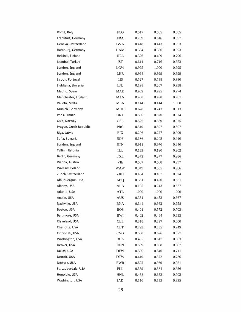
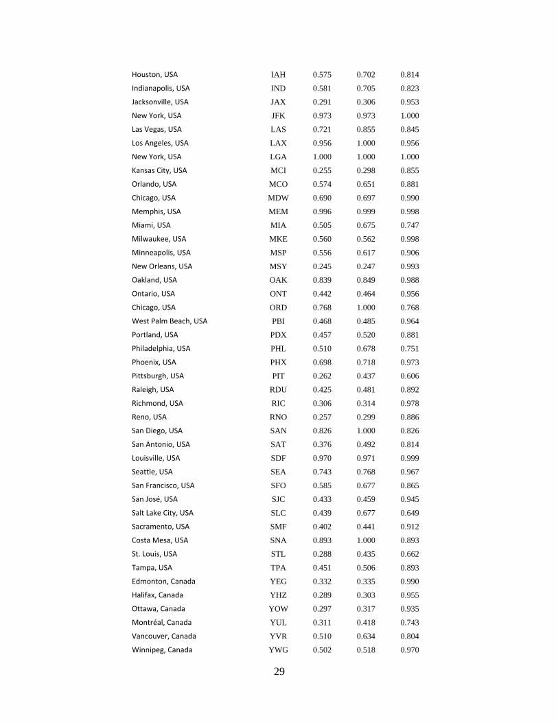
Table A2: Technical efficiency scores for all airports other than Latin American airports included in our sample (data from the ATRS Airport Benchmarking Report)
Airport IATA Code
CRS VRS Scale
Efficiency
Auckland, New Zealand AKL 0.648 0.879 0.737
Bangkok, Thailand BKK 0.935 0.951 0.983
Brisbane, Australia BNE 0.655 0.718 0.912
Guangzhou, China CAN 0.651 0.665 0.979
Jakarta, Indonesia CGK 0.854 0.867 0.985
Christchurch, New Zealand CHC 0.357 0.371 0.964
Chiang Mai, Thailand CNX 0.245 0.329 0.745
Haikou, China HAK 0.366 0.421 0.870
Hat Yai, Thailand HDY 0.134 0.208 0.645
Hong Kong, Hong Kong HKG 1.000 1.000 1.000
Phuket, Thailand HKT 0.393 0.528 0.743
Seoul, Korea ICN 0.962 0.962 1.000
Osaka, Japan KIX 0.743 1.000 0.743
Kuala Lumpur, Malaysia KUL 0.652 0.657 0.992
Macau MFM 0.465 0.844 0.555
Tokyo, Japan NRT 0.860 0.876 0.982
Penang, Malaysia PEN 0.386 0.898 0.430
Shanghai, China PVG 0.909 0.931 0.976
Seoul, South Korea SEL 0.618 0.619 0.999
Singapore, Singapore SIN 0.927 0.934 0.993
Sydney, Australia SYD 0.828 0.837 0.991
Shenzhen, China SZX 0.721 0.949 0.760
Xiamen, China XMN 1.000 1.000 1.000
Amsterdam, Netherlands AMS 0.637 0.856 0.745
Stockholm, Sweden ARN 0.410 0.453 0.905
Athens, Greece ATH 0.464 0.471 0.987
Barcelona, Spain BCN 0.731 0.763 0.959
Birmingham, England BHX 0.365 0.367 0.994
Brussels, Belgium BRU 0.370 0.419 0.881
Bratislava, Slovak BTS 0.102 0.105 0.971
Budapest, Hungary BUD 0.331 0.332 0.996
Paris, France CDG 0.826 0.922 0.896
Cologne, Germany CGN 0.299 0.388 0.771
Rome, Italy CIA 0.488 0.612 0.797
Copenhagen, Denmark CPH 0.369 0.385 0.960
Dublin, Ireland DUB 0.457 0.468 0.976
Dusseldorf, Germany DUS 0.324 0.341 0.951
Edinburgh, Scotland EDI 0.693 0.799 0.868
28
Rome, Italy FCO 0.517 0.585 0.885
Frankfurt, Germany FRA 0.759 0.846 0.897
Geneva, Switzerland GVA 0.418 0.443 0.953
Hamburg, Germany HAM 0.384 0.386 0.993
Helsinki, Finland HEL 0.326 0.409 0.796
Istanbul, Turkey IST 0.611 0.716 0.853
London, England LGW 0.995 1.000 0.995
London, England LHR 0.998 0.999 0.999
Lisbon, Portugal LIS 0.527 0.538 0.980
Ljubljana, Slovenia LJU 0.198 0.207 0.958
Madrid, Spain MAD 0.969 0.995 0.974
Manchester, England MAN 0.488 0.498 0.981
Valleta, Malta MLA 0.144 0.144 1.000
Munich, Germany MUC 0.678 0.743 0.913
Paris, France ORY 0.556 0.570 0.974
Oslo, Norway OSL 0.526 0.539 0.975
Prague, Czech Republic PRG 0.319 0.397 0.807
Riga, Latvia RIX 0.206 0.227 0.909
Sofia, Bulgaria SOF 0.186 0.205 0.910
London, England STN 0.911 0.970 0.940
Tallinn, Estonia TLL 0.163 0.180 0.902
Berlin, Germany TXL 0.372 0.377 0.986
Vienna, Austria VIE 0.507 0.508 0.997
Warsaw, Poland WAW 0.349 0.355 0.986
Zurich, Switzerland ZRH 0.434 0.497 0.874
Albuquerque, USA ABQ 0.351 0.420 0.851
Albany, USA ALB 0.195 0.243 0.827
Atlanta, USA ATL 1.000 1.000 1.000
Austin, USA AUS 0.381 0.453 0.867
Nashville, USA BNA 0.344 0.362 0.958
Boston, USA BOS 0.401 0.572 0.703
Baltimore, USA BWI 0.402 0.484 0.835
Cleveland, USA CLE 0.318 0.397 0.800
Charlotte, USA CLT 0.793 0.835 0.949
Cincinnati, USA CVG 0.550 0.626 0.877
Washington, USA DCA 0.495 0.617 0.803
Denver, USA DEN 0.599 0.898 0.667
Dallas, USA DFW 0.596 0.840 0.711
Detroit, USA DTW 0.419 0.572 0.736
Newark, USA EWR 0.892 0.939 0.951
Ft. Lauderdale, USA FLL 0.559 0.584 0.956
Honolulu, USA HNL 0.458 0.653 0.702
Washington, USA IAD 0.510 0.553 0.935
29
Houston, USA IAH 0.575 0.702 0.814
Indianapolis, USA IND 0.581 0.705 0.823
Jacksonville, USA JAX 0.291 0.306 0.953
New York, USA JFK 0.973 0.973 1.000
Las Vegas, USA LAS 0.721 0.855 0.845
Los Angeles, USA LAX 0.956 1.000 0.956
New York, USA LGA 1.000 1.000 1.000
Kansas City, USA MCI 0.255 0.298 0.855
Orlando, USA MCO 0.574 0.651 0.881
Chicago, USA MDW 0.690 0.697 0.990
Memphis, USA MEM 0.996 0.999 0.998
Miami, USA MIA 0.505 0.675 0.747
Milwaukee, USA MKE 0.560 0.562 0.998
Minneapolis, USA MSP 0.556 0.617 0.906
New Orleans, USA MSY 0.245 0.247 0.993
Oakland, USA OAK 0.839 0.849 0.988
Ontario, USA ONT 0.442 0.464 0.956
Chicago, USA ORD 0.768 1.000 0.768
West Palm Beach, USA PBI 0.468 0.485 0.964
Portland, USA PDX 0.457 0.520 0.881
Philadelphia, USA PHL 0.510 0.678 0.751
Phoenix, USA PHX 0.698 0.718 0.973
Pittsburgh, USA PIT 0.262 0.437 0.606
Raleigh, USA RDU 0.425 0.481 0.892
Richmond, USA RIC 0.306 0.314 0.978
Reno, USA RNO 0.257 0.299 0.886
San Diego, USA SAN 0.826 1.000 0.826
San Antonio, USA SAT 0.376 0.492 0.814
Louisville, USA SDF 0.970 0.971 0.999
Seattle, USA SEA 0.743 0.768 0.967
San Francisco, USA SFO 0.585 0.677 0.865
San José, USA SJC 0.433 0.459 0.945
Salt Lake City, USA SLC 0.439 0.677 0.649
Sacramento, USA SMF 0.402 0.441 0.912
Costa Mesa, USA SNA 0.893 1.000 0.893
St. Louis, USA STL 0.288 0.435 0.662
Tampa, USA TPA 0.451 0.506 0.893
Edmonton, Canada YEG 0.332 0.335 0.990
Halifax, Canada YHZ 0.289 0.303 0.955
Ottawa, Canada YOW 0.297 0.317 0.935
Montréal, Canada YUL 0.311 0.418 0.743
Vancouver, Canada YVR 0.510 0.634 0.804
Winnipeg, Canada YWG 0.502 0.518 0.970
30
Calgary, Canada YYC 0.732 0.745 0.983
Toronto, Canada YYZ 0.371 0.484 0.765
Table A3: Average TE scores and scale efficiency by region (2005-2006 average) Model with 3 Outputs (passengers, cargo and aircraft movements) and 2 Inputs (runways and employees)
World Region
Technical efficiency Returns to scale diagnosis
(% of observations)
CRS VRS Scale IRS CRS DRS
Latin America 0.283 0.399 0.796 63.6 6.8 29.5
Asia 0.477 0.528 0.901 38.5 2.6 59.0
Europe 0.454 0.512 0.886 47.0 7.6 45.5
Canada & US 0.443 0.491 0.911 36.8 5.6 57.6
All 0.425 0.487 0.885 43.8 5.8 50.4
31
Table A4: LAC airports TFPC (Annual %)
Year Argentina Brazil Chile Colombia Costa Rica
AEP EZE FTE BSB CGH GIG GRU MAO VCP SCL BAQ CLO SJO
1995-1996 - - - 9.9 8.4 4.1 11.7 -21.5 -4.4 - - -
1996-1997 - - - 23.6 20.3 9.3 5.3 -3.0 9.0 - - -
1997-1998 - - - 9.6 17.7 8.8 0.2 15.2 8.5 - -32.1 -
1998-1999 - - - -1.5 9.1 -22.7 -2.5 4.0 -8.4 - -12.7 -
1999-2000 - - - 8.2 12.9 5.6 1.2 5.9 20.0 11.8 9.2 -
2000-2001 -40.1 -24.8 - -1.5 13.1 -1.6 -5.7 -7.6 -1.7 -9.7 -27.8 -
2001-2002 -15.8 -41.9 - 10.0 3.7 -8.2 -1.4 6.2 -22.7 -10.4 -0.9 -23.7 57.0
2002-2003 2.8 22.2 - -4.4 -16.3 -16.5 2.3 -2.5 -20.0 3.7 -9.7 15.3 -5.0
2003-2004 5.9 20.0 60.3 12.1 -84.2 6.5 2.6 9.6 0.6 2.8 -2.8 -17.2 1.2
2004-2005 -2.5 -9.0 14.6 -39.0 9.0 43.7 9.4 2.0 -6.6 5.7 3.0 -5.2 -0.6
2005-2006 -9.3 5.2 3.9 -11.0 -15.4 2.3 -6.7 3.0 -18.6 -2.2 4.5 -2.6 -4.1
2006-2007 -5.5 1.9 19.7 9.2 -26.5 16.9 6.0 12.8 26.5 -15.2 1.3 5.9 3.6
Note: In bold are indicated the year of changes in capital stock, either in the number of runways or in the number of boarding bridges.
32
Table A4 (continued): LAC airports TFPC (Annual %)
Year Ecuador
El Salvador
Mexico Panama Peru Dom. Rep
GYE SAL CUN GDL MEX MTY PTY LIM SDQ
1995-1996 - - - - - - - - -
1996-1997 - - - - - - - - -
1997-1998 - - - - - - - - -
1998-1999 - - - - - - - - -
1999-2000 - - 18.5 - 0.8 -1.2 - - -
2000-2001 - - -3.3 - -9.9 -5.9 - - -
2001-2002 - 7.4 1.9 - 0.4 18.0 - - -
2002-2003 - -1.8 10.4 -6.1 2.2 14.1 - - -
2003-2004 - 12.4 10.2 5.1 6.0 1.7 9.0 - -
2004-2005 - -0.6 -8.2 -13.9 3.3 3.8 6.8 - -9.1
2005-2006 -28.2 -0.9 -2.1 12.3 5.5 -0.5 -20.3 9.6 -10.5
2006-2007 8.1 -4.7 -1.7 11.3 -6.9 14.2 6.3 9.8 2.0
Note: In bold are indicated the year of changes in capital stock, either in the number of runways or in the number of boarding bridges.
33
Methodological Appendix
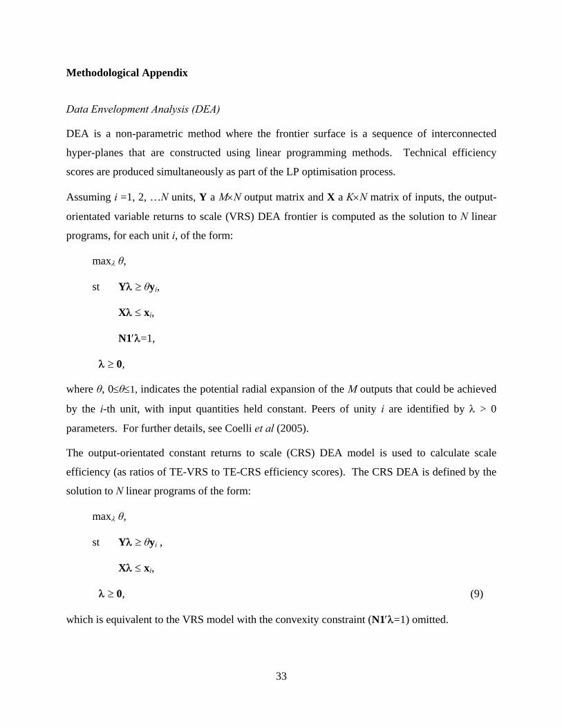
Data Envelopment Analysis (DEA)
DEA is a non-parametric method where the frontier surface is a sequence of interconnected
hyper-planes that are constructed using linear programming methods. Technical efficiency
scores are produced simultaneously as part of the LP optimisation process.
Assuming i =1, 2, …N units, Y a MN output matrix and X a KN matrix of inputs, the output-
orientated variable returns to scale (VRS) DEA frontier is computed as the solution to N linear
programs, for each unit i, of the form:
max θ,
st Y θyi,
X xi,
N1=1,
0,
where θ, 0θ1, indicates the potential radial expansion of the M outputs that could be achieved
by the i-th unit, with input quantities held constant. Peers of unity i are identified by > 0
parameters. For further details, see Coelli et al (2005).
The output-orientated constant returns to scale (CRS) DEA model is used to calculate scale
efficiency (as ratios of TE-VRS to TE-CRS efficiency scores). The CRS DEA is defined by the
solution to N linear programs of the form:
max θ,
st Y θyi ,
X xi,
0, (9)
which is equivalent to the VRS model with the convexity constraint (N1=1) omitted.