The Astrophysical Journal, 773:47 (16pp), 2013 August 10 doi:10.1088/0004-637X/773/1/47C© 2013. The American Astronomical Society. All rights reserved. Printed in the U.S.A.

MEASURING THE ROTATIONAL PERIODS OF ISOLATED MAGNETIC WHITE DWARFS

Carolyn S. Brinkworth1,2, Matthew R. Burleigh3, Katherine Lawrie3, Thomas R. Marsh4, and Christian Knigge51 Spitzer Science Center, California Institute of Technology, Pasadena, CA 91125, USA

2 NASA Exoplanet Science Institute, California Institute of Technology, Pasadena, CA 91125, USA3 Department of Physics and Astronomy, University of Leicester, Leicester LE1 7RH, UK4 Department of Physics and Astronomy, University of Warwick, Coventry CV4 7AL, UK

5 School of Physics and Astronomy, University of Southampton, Southampton SO17 1BJ, UKReceived 2012 March 27; accepted 2013 June 22; published 2013 July 24

ABSTRACT

We present time-series photometry of 30 isolated magnetic white dwarfs, surveyed with the Jacobus KapteynTelescope between 2002 August and 2003 May. We find that 9 were untestable due to varying comparison stars,but of the remaining 21, 5 (24%) are variable with reliably derived periods, while a further 9 (43%) are seen to varyduring our study, but we were unable to derive the period. We interpret the variability to be the result of rotation ofthe objects. We find no correlation between rotation period and mass, temperature, magnetic field, or age. We havefound variability in 9 targets with low magnetic field strengths and temperatures low enough for partially convectiveatmospheres, which we highlight as candidates for polarimetry to search for starspots. Most interestingly, we havefound variability in one target, PG1658+441, which has a fully radiative atmosphere in which conventional starspotscannot form, but a magnetic field strength that is too low to cause magnetic dichroism. The source of variability inthis target remains a mystery.

Key words: stars: magnetic field – stars: rotation – starspots – surveys – white dwarfs

Online-only material: color figures

1. INTRODUCTION

Up to approximately 600 isolated white dwarfs, composing∼3% of the currently known population, have measured mag-netic fields (10 kG < B < 1000 MG; e.g., Wickramasinghe& Ferrario 2000; Schmidt et al. 2003; Vanlandingham et al.2005; Kawka et al. 2007; Kepler et al. 2013; Kleinman et al.2013). Holberg et al. (2008) have cataloged 16 magnetic de-generates among 126 white dwarfs within 20 pc, suggestingthe fraction among the total population is at least 13%. Kawkaet al. (2007) list 9 magnetic stars from 43 white dwarfs in themore statistically complete sample within 13 pc, resulting inan incidence of 21% ± 8%. Furthermore, Jordan et al. (2007)have searched for magnetic fields as low as 1 kG in a num-ber of nearby white dwarfs, and estimate the fraction with suchweak fields as 11%–15%, similar to the incidence of higher fieldstrengths.

The mass distribution of magnetic white dwarfs impliesthat they have a higher average mass than their non-magneticcounterparts (e.g., Liebert et al. 2005). This bias may providea clue as to the origin of their magnetic fields. Some of thesestars may be the direct descendants of high-mass main-sequencemagnetic Ap and Bp stars (M > 2 M�; Wickramasinghe &Ferrario 2005). However, Kawka & Vennes (2004) argued thatthe present space density of Ap/Bp progenitors is insufficientto account for the density of known magnetic white dwarfs inthe solar neighborhood.

Liebert et al. (2005) noted that although ∼25% of interactingcataclysmic variable (CV) systems contain a magnetic whitedwarf, there are no known examples of detached binariesconsisting of a main-sequence star and a magnetic white dwarf.In other words, there are no known close binary progenitorsof magnetic CVs. Tout et al. (2008) explain this discrepancyas the result of the common envelope evolution that precedesthe formation of a detached close binary. During a common

envelope, a low-mass star and the eventual white dwarf arebrought close together as the orbit shrinks through frictionand the loss of angular momentum. A CV later forms whenthe emergent close binary is brought into contact by magneticbraking or gravitational radiation. Tout et al. (2008) propose thatthe magnetic field on the white dwarf is generated by differentialrotation and convection within the common envelope. Thesmaller the orbital separation at the end of the common envelopephase, the stronger the magnetic field on the white dwarf.Magnetic CVs are systems which emerge from the commonenvelope very close to semi-detached contact. The isolated,single magnetic white dwarfs are the result of common envelopebinaries that merged. Thus, Tout et al. (2008) propose that allhighly magnetic white dwarfs, whether single or in magneticCVs, are the result of close binary evolution. This scenario offorming high-field magnetic white dwarfs through mergers issupported by the more recent work of Nordhaus et al. (2011)and Garcia-Berro et al. (2012). In this picture, low-field stars(< a MG) may still be the descendants of single main-sequenceprogenitors.

Measuring rotational periods in non-magnetic white dwarfs isnotoriously difficult due to the heavy broadening of the spectrallines by the strong gravitational field (Berger et al. 2005). Mag-netic white dwarfs, on the other hand, display spectroscopic and/or photometric variability which allows much easier identifica-tion of their spin periods. The rotation rates allow investigationof angular momentum transfer from the core to the envelope andlarge-scale angular momentum loss during post-main-sequenceevolution, for both magnetic white dwarfs and white dwarfs ingeneral, and for investigation of the formation scenarios.

Spectroscopic variability in magnetic white dwarfs is gen-erally caused by variations in the surface field strength, whichcan be observed in the motion of the Zeeman-split componentsof the Balmer lines. Photometric variability can be caused bythe dependence of the continuum opacity on the surface field

1

The Astrophysical Journal, 773:47 (16pp), 2013 August 10 Brinkworth et al.

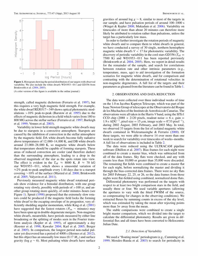
Figure 1. Histogram showing the period distribution of our targets with observedvariability. We also include the white dwarfs WD1953−011 and GD356 fromBrinkworth et al. (2004, 2005).

(A color version of this figure is available in the online journal.)

strength, called magnetic dichroism (Ferrario et al. 1997), butthis requires a very high magnetic field strength. For example,the white dwarf REJ0317−349 shows optical photometric mod-ulations >10% peak-to-peak (Barstow et al. 1995) due to theeffects of magnetic dichroism in a field which varies from 180 to800 MG across the stellar surface (Ferrario et al. 1997; Burleighet al. 1999; Vennes et al. 2003).

Variability in lower field strength magnetic white dwarfs maybe due to starspots in a convective atmosphere. Starspots arecaused by the inhibition of convection in the stellar atmosphereby the magnetic field. DA white dwarfs become fully radiativeabove temperatures of 12,000–14,000 K, and DB white dwarfsaround 23,000–28,000 K, so magnetic white dwarfs belowthat temperature should be capable of forming starspots. Theseareas of reduced convection are cooler (and therefore darker)than the surrounding atmosphere, leading to a drop in theobserved magnitude of the star as the spots rotate into view.The effect is evident in the Teff ≈ 8000 K, B ≈ 70 kGstar WD1953−011, which shows a sinusoidal variation of≈2% peak-to-peak amplitude every 1.44 days due to a starspotcovering ∼10% of the surface (Maxted et al. 2000; Brinkworthet al. 2005; Valyavin et al. 2011).

Previously measured magnetic white dwarf rotational peri-ods show evidence for a bimodal distribution, with one grouprotating very slowly, possibly with periods of >100 yr, and an-other group rotating more quickly, of order minutes–hours (seeFigure 1). Spruit (1998) proposed that the extremely slow rota-tors could be produced if the magnetic field locks the formingwhite dwarf to the escaping envelope of its progenitor, very ef-ficiently shedding angular momentum, while King et al. (2001)have suggested that the fastest rotators (Prot ∼ minutes) mayhave been spun up in double-degenerate mergers. Non-magneticwhite dwarfs, meanwhile, have periods measured by either linebroadening or the splitting of modes seen in the Fourier trans-form analysis (Kepler et al. 1995), of approximately a day(Koester et al. 1998; Kawaler 2004; Karl et al. 2005; Bergeret al. 2005). In comparison, the longest period non-radial pul-sator yet discovered has a period of 4000 s (Hermes et al. 2012),but this object has an unusually low mass (0.17 M�) and surfacegravity (log g ∼ 6). Most pulsating white dwarfs have surface

gravities of around log g ∼ 8, similar to most of the targets inour sample, and have pulsation periods of around 100–1000 s(Winget & Kepler 2008; Mukadam et al. 2006). Variability ontimescales of more than about 20 minutes can therefore morelikely be attributed to rotation rather than pulsations, unless thetarget has a particularly low mass.

In order to further investigate the rotation periods of magneticwhite dwarfs and to compare them to white dwarfs in general,we have conducted a survey of 30 single, northern hemispheremagnetic white dwarfs V < 17 for photometric variability. Thediscovery of periodic variability in the cool stars GD356 (Teff =7500 K) and WD1953−011 has been reported previously(Brinkworth et al. 2004, 2005). Here, we report in detail resultsfor the remainder of the sample, and search for correlationsbetween rotation rate and other intrinsic parameters (e.g.,temperature, mass, age) to aid investigation of the formationscenarios for magnetic white dwarfs, and for comparison andcontrasting with the determination of rotational velocities innon-magnetic degenerates. A full list of the targets and theirparameters as gleaned from the literature can be found in Table 1.

2. OBSERVATIONS AND DATA REDUCTION

The data were collected over three individual weeks of timeon the 1.0 m Jacobus Kapteyn Telescope, which was part of theIsaac Newton Group of telescopes at the Observatorio del Roquede los Muchachos of the Instituto de Astrofisica de Canarias. Theobservations were all taken in the Harris V band, using the SITe1CCD chip (2088 × 2120 pixels, readout noise = 6 e, gain =1.9 e ADU−1, pixel size = 15 μm, image scale = 0.′′33 pixel−1),during 2002 August, 2003 February, and 2003 May. In total,we observed 33 targets from the list of isolated magnetic whitedwarfs contained in Wickramasinghe & Ferrario (2000). Ofthese targets, we were able to observe 14 over more than oneweek to search for variability over timescales of weeks–months.A full list of observations is included in Table 2.

The data were reduced using the ULTRACAM pipelinesoftware (Dhillon et al. 2007). Bias frames for each night werecombined to create a master bias, which was subtracted fromall of the data frames. Sky flats were checked, and any withcounts less than 10,000 or greater than 35,000 were discarded.The remaining flat fields were combined to create a master flatfor each night, before normalizing the master and dividing itthrough the bias-corrected data frames. There were no sky flatsfor 2003 February 22, 25, or 26, so the data frames from thosenights were flat-fielded using combined, normalized dome flats.

Differential photometry was performed on the targets withrespect to at least two bright comparison stars in the field, andusually three or four. We used variable apertures (allowingthe apertures to vary with the fitted FWHM of the source,so compensating for changes in the observing conditions). Weextracted fluxes by summing counts in excess of the sky level,which was estimated by taking the mean after rejecting pointsmore than 3σ away from the mean.

The stable comparisons were combined to create a singlebright master comparison, which we divided into the target tocalculate the differential photometry. Results are given in dif-ferential flux and all times have been converted to HeliocentricJulian Date.

2.1. Detection of Variability

We used a “floating mean” periodogram (e.g., Cumming et al.1999; Morales-Rueda et al. 2003) to search for periodicity in

2

The Astrophysical Journal, 773:47 (16pp), 2013 August 10 Brinkworth et al.

Table 1Magnetic White Dwarf Parameters from the Literature

Target White Dwarf Name Bp Teff Mass Comp V Age Plit Refs(MG) (K) (M�) (mag) (Gyr)

EUVE J1439+75.0 WD1440+753 14.8 39500 0.9–1.2 H; DD 15.4 0.005–0.3 . . . 44, 9G99−37 WD0548−001 10–20: 6070 0.69 He 14.6 3.90 4.117 hr 1, 9, 50, 51G99−47 WD0533+053 20 5790 0.71 H 14.1 3.97 1 hr 1, 9, 10, 11, 12, 55G111−49 WD0756+437 300–377 8500 1.07 H 16.3 . . . . . . 3, 9, 15, 45G141−2 WD1818+126 3: 6340 0.26 H; DD 15.9 0.93 years? 1, 34, 22G158−45 WD0011−134 16.7 6010 0.71 H 15.9 3.43 11 hr–1 day 1, 3G183−35 WD1814+248 14: 6500 . . . H, He: 16.9 . . . 50 minutes–few yr 3, 28G195−19 WD0912+536 100 7160 0.75 He 13.8 2.54 1.33 days 1, 17, 18G217−037 WD0009+501 �0.2 6540 0.74 H 14.4 3.58 2–20 hr 1, 2, 48, 55G227−28 WD1820+609 �0.1 4780 0.48 H 15.7 4.68 . . . 1, 3, 55G227−35 WD1829+547 170–180 6280 0.90 H 15.5 4.76 �100 yr 12, 1, 35G234−4 WD0728+642 0.1–0.4 4500 0.58 H, He 16.3 7.58 . . . 3, 55G240−72 WD1748+708 �100 5590 0.81 He 14.2 5.69 �100 yr: 1, 33, 17, 55G256−7 WD1309+853 4.9 5600 . . . H 16.0 . . . . . . 28GD77 WD0637+478 1.2 14000 0.74: H 14.8 . . . . . . 9, 13, 14GD90 WD0816+376 9 11000 0.60 H 15.6 0.47 . . . 3, 14, 16, 52, 53GD229 WD2010+310 500 16000 �1.0 He 14.8 . . . �100 yr 37, 38, 33, 39Grw+70◦8247 WD1900+705 320 12070 0.95 He 13.2 0.95 �100 yr 1, 36, 20, 55HE0107−0158 WD0107−019 10:-30: . . . . . . He; Bin 16.4: . . . . . . 4, 5HE1045−0908 WD1045−091 10–75 10000 . . . H 16.7 . . . 2–11 hr 5, 25, 54HE1211−1707 WD1211−171 50 12–23000 . . . He 16.8 . . . ∼2 hr 5, 26LB8915 WD0853+163 0.1–1 21-27000 . . . H+He 15.8 . . . . . . 3, 49LB11146 WD0945+246 670 16000 0.9 H, He; DD 14.3 . . . . . . 41, 42, 43LHS2273 WD1026+117 ∼10 7160 0.59 H 16.6 1.51 . . . 22, 23LHS5064 WD 0257+080 �0.2 6680 0.57 H 15.9 1.60 . . . 1, 9LP907−037 WD1350+090 �0.1 9520 0.83 H 14.6 1.32 . . . 30, 2, 47PG0136+251 WD0136+251 �0.1 39640 1.20 H 15.8: 0.75 . . . 6, 47PG1015+015 WD1015+014 50–90 10000 . . . H 16.3 . . . 98.7 minutes 19, 20, 21, 46PG1031+234 WD1031+234 500–1000 15000 0.93 H 15.8 0.55 3.40 hr 24, 47PG1533−057 WD1533−057 31 20000 0.94 H 15.3 0.25 ∼1 day 31, 23, 47PG1658+441 WD1658+441 3.5 30510 1.31 H 14.6 0.38 . . . 32, 6, 47PG2329+267 WD2329+267 2.3 11730 1.18 H 15.3 2.04 . . . 40, 47SBSS1349+545 WD1349+545 760 11000: . . . H 16.4 . . . . . . 29

References. (1) Bergeron et al. 2001; (2) Schmidt & Smith 1995; (3) Putney 1997; (4) Reimers et al. 1998; (5) Schmidt et al. 2001; (6) Schmidt et al. 1992a;(7) Friedrich et al. 1996; (8) Dupuis et al. 2002; (9) Wickramasinghe & Ferrario 2000; (10) Wickramasinghe & Martin 1979; (11) Greenstein & McCarthy 1985;(12) Putney & Jordan 1995; (13) Schmidt et al. 1992b; (14) Guseinov et al. 1983b; (15) Guseinov et al. 1983a; (16) Angel et al. 1974; (17) Angel 1978; (18) Liebert1976; (19) Wickramasinghe & Cropper 1988; (20) Schmidt & Norsworthy 1991; (21) Schmidt et al. 2003; (22) Bergeron et al. 1997; (23) Schmidt & Smith 1995;(24) Schmidt et al. 1986; (25) Reimers et al. 1994; (26) Reimers et al. 1996; (27) Liebert et al. 2003; (28) Putney 1995; (29) Liebert et al. 1994; (30) Koester et al.1998; (31) Liebert et al. 1985; (32) Liebert et al. 1983; (33) Berdyugin & Pirola 1999; (34) Greenstein 1986; (35) Cohen et al. 1993; (36) Wickramasinghe & Ferrario1988; (37) Wickramasinghe et al. 2002; (38) Green & Liebert 1981; (39) Schmidt et al. 1996; (40) Moran et al. 1998; (41) Liebert et al. 1993; (42) Glenn et al. 1994;(43) Schmidt et al. 1998; (44) Vennes et al. 1999; (45) Kulebi et al. 2009; (46) Euchner et al. 2006; (47) Liebert et al. 2005; (48) Valyavin et al. 2005; (49) Wesemaelet al. 2001; (50) Bues & Pragal 1989; (51) Dufour et al. 2005; (52) Jordan et al. 2001; (53) Limoges & Bergeron 2010; (54) Euchner et al. 2005; (55) Sion et al. 2009.

each of the targets. This is a generalization of the Lomb–Scargleperiodogram (Lomb 1976; Scargle 1982) and involves fitting thedata with a sinusoid plus constant of the form

A + B sin[2πf (t − t0)],

where f is the frequency and t is the observation time. Wesearched frequencies from 0.001 to 100 cycles day−1, withan oversampling factor of 10. For the normalization of theperiodogram, we use the weighted sum of squares of residualsto the best-fit sinusoid, χ2(ω0), as described in Cumming et al.(1999). The advantage of the floating mean periodogram overthe Lomb–Scargle periodogram is that it treats the constant,A, as an extra free parameter rather than fixing the zero-pointand then fitting a sinusoid, i.e., it allows the zero-point to“float” during the fit. It also takes uncertainties into account,while the Lomb–Scargle periodogram ignores them. Unlike the

Lomb–Scargle periodogram and running Fourier transforms,the floating-mean periodogram is robust when the number ofobservations is small, the sampling is uneven, and the derivedperiod is longer than the baseline of the observations (Cumminget al. 1999). The resultant periodogram is an inverted χ2 plot ofthe fit at each frequency.

To test the significance of the variability, we carried out twofurther tests. Firstly, we suspected that the formal errors wereunderestimated, so we re-scaled the error bars to give a reducedχ2 = 1 for the global minimum in the periodogram. We thencompared the χ2 values from the periodogram to the χ2 of aconstant fit, using a change in χ2 of 16 (equivalent to 4σ ) as thethreshold for a target to be initially classified as variable. A listof the reduced χ2 values for all of the targets can be found inTable 3. Having established that the formal errors failed to coverthe scatter in the data, we compared the level of variability in thetarget to the level seen in the comparison stars. We compared the

3

The Astrophysical Journal, 773:47 (16pp), 2013 August 10 Brinkworth et al.

Table 2Observing Log for Our White Dwarf Sample

Target White Dwarf Name Epoch Number of Frames

G217−037 WD0009+501 2002 Aug 198G158−45 WD0011−134 2002 Aug 76HE0107−0158 WD0107−019 2002 Aug 60PG0136+251 WD0136+251 2002 Aug 25LHS5064 WD 0257+080 2003 Feb 33G99−47 WD0533+053 2003 Feb 69G99−37 WD0548−001 2003 Feb 23GD77 WD0637+478 2003 Feb 45G234−4 WD0728+642 2003 Feb 18G111−49 WD0756+437 2003 Feb 100GD90 WD0816+376 2003 Feb 18LB8915 WD0853+163 2003 Feb 30G195−19 WD0912+536 2003 Feb 33

2003 May 40LB11146 WD0945+246 2003 Feb 18PG1015+015 WD1015+014 2003 Feb 26LHS2273 WD1026+117 2003 May 35PG1031+234 WD1031+234 2003 Feb 25HE1045−0908 WD1045−091 2003 Feb 47HE1211−1707 WD1211−171 2003 Feb 21

2003 May 22G256−7 WD1309+853 2003 May 37SBSS1349+545 WD1349+545 2003 May 51LP907−037 WD1350+090 2003 May 30EUVE J1439+75.0 WD1440+753 2002 Aug 20

2003 Feb 132003 May 5

PG1533−057 WD1533−057 2002 Aug 682003 Feb 212003 May 306

PG1658+441 WD1658+441 2002 Aug 552003 May 10

G240−72 WD1748+708 2002 Aug 602003 May 10

G183−35 WD1814+248 2002 Aug 782003 May 40

G141−2 WD1818+126 2002 Aug 66G227−28 WD1820+609 2002 Aug 40

2003 May 10G227−35 WD1829+547 2002 Aug 55

2003 May 10Grw+70◦8247 WD1900+705 2002 Aug 125GD229 WD2010+310 2002 Aug 55

2003 May 10PG2329+267 WD2329+267 2002 Aug 153

2003 May 5

Note.Targets are listed in order of R.A.

rms of the normalized target differential light curve to the rms ofthe normalized differential light curves of the comparisons. Forthose with target rms comparable to the comparison rms, we rana periodogram on the comparison stars to test for periodicity inthe comparison star data. Those targets that display variabilityon the same level as the comparisons, with similar significancein the periodogram compared to constant fits, are listed asnon-variable. Finally, we ran Monte Carlo simulations withGaussian noise to estimate the false alarm probability (FAP)for each target, as outlined in detail in Cumming et al. (1999).The results of the FAP tests can be found in Table 3. The FAP wascalculated as the fraction of 1000 randomly generated datasets(sampled at the observed times about the observed mean fluxwith random Gaussian noise) that would cause a mean power

signal in the periodogram greater than the mean power foundfrom our observed data. We set the significance threshold to anFAP of 1% (FAP < 0.01).

The final classification of variable versus non-variable wasmade using a combination of the above methods. The identi-fication of the best-fitting period for the variable targets wasmade by examining the change in the χ2 between the globalminimum and the next best frequency. Lines marking changesin χ2 of 1, 4, and 9 (equivalent to 1σ , 2σ , and 3σ , assumingone fitted parameter) are marked on the periodograms for eachtarget. The 2σ errors are quoted in the text, and a change inχ2 of 9 (3σ ) between two minima was taken as a significantlybetter fit.

For some of the targets (e.g., LB8915) there were a number oflocal aliases within the 3σ uncertainty. In these cases, we ran aLomb–Scargle periodogram on the data, which ignores the errorbars on the data, giving us an unweighted least-squares fittingas an alternative test. We then folded the light curves on at leastthe best two periods identified in the two periodograms. Themost likely periods for each of the targets are quoted in Table 3,along with the 2σ uncertainties.

3. RESULTS

Of the 33 stars we observed, two were identified in theliterature as binary systems, and one is not believed to bemagnetic. These stars were discarded from our survey, leavingus with 30 isolated magnetic white dwarfs. Of these 30 targets, 5displayed photometric variability with a measurable period, i.e.,a minimum in the periodogram that was significantly better thanthe next-best-fitting period. A further 9 displayed significantvariability, but we were unable to differentiate between a numberof possible aliases. We found no evidence for variability in theremaining targets, but provide upper limits.

3.1. Targets Displaying Variability with a Measured Period

3.1.1. G111−49 (WD0756+437)

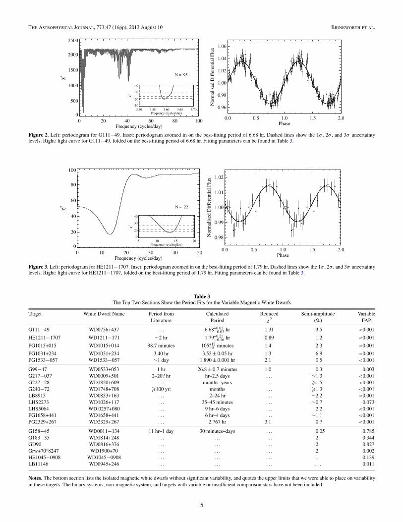
The magnetic nature of G111−49 was discovered by Putney(1995), who reclassified its spectral type as an H-rich magneticwhite dwarf and reported strong circular polarization (Vmax =9%) and a field strength of ∼220 MG. Putney (1995) also notedthat G111−49 has been classified in the literature as a varietyof different white dwarf spectral types since Greenstein et al.(1977) and suggested that this could be indicative of rotation.More recently, Kulebi et al. (2009) measured the field strengthfrom a Sloan optical spectrum as 300 MG (centered magneticdipole case) or 377 MG if the dipole is shifted by 0.23 stellarradii along the dipole axis. We have discovered photometricvariability in G111−49 with a peak-to-peak amplitude of ∼7%and a period of 6.68 +0.02

−0.03 hr. The periodogram is in Figure 2,which shows that the difference in χ2 between the fits of thebest and second-best periods (Δχ2) is more than 200. The lightcurve, folded on the best period, is also shown in Figure 2.

3.1.2. HE1211−1707 (WD1211−171)

Reimers et al. (1996) reported time-variable absorption fea-tures in the spectrum of HE1211−1707, and Schmidt et al.(2001) found the rotational period from optical spectra and cir-cular spectropolarimetry to be ∼2 hr. Schmidt et al. (2001)and Jordan et al. (2001) also independently showed thatHE1211−1707 is a rare He-rich magnetic degenerate. We ob-served HE1211−1707 in 2003 February, but failed to find any

4

The Astrophysical Journal, 773:47 (16pp), 2013 August 10 Brinkworth et al.

3.50 3.55 3.60 3.65 3.70Frequency (cycles/day)

110

120

130

140

χ2

0 20 40 60 80 100Frequency (cycles/day)

0

500

1000

1500

2000

2500

χ2 N = 95

0.0 0.5 1.0 1.5 2.0Phase

0.96

0.98

1.00

1.02

1.04

1.06

Nor

mal

ised

Dif

fere

ntia

l Flu

x

Figure 2. Left: periodogram for G111−49. Inset: periodogram zoomed in on the best-fitting period of 6.68 hr. Dashed lines show the 1σ , 2σ , and 3σ uncertaintylevels. Right: light curve for G111−49, folded on the best-fitting period of 6.68 hr. Fitting parameters can be found in Table 3.

5 10 15 20Frequency (cycles/day)

10

20

30

40

χ2

0 10 20 30 40 50Frequency (cycles/day)

0

20

40

60

80

100

χ2 N = 22

0.0 0.5 1.0 1.5 2.0Phase

0.98

0.99

1.00

1.01

1.02

Nor

mal

ised

Dif

fere

ntia

l Flu

x

Figure 3. Left: periodogram for HE1211−1707. Inset: periodogram zoomed in on the best-fitting period of 1.79 hr. Dashed lines show the 1σ , 2σ , and 3σ uncertaintylevels. Right: light curve for HE1211−1707, folded on the best-fitting period of 1.79 hr. Fitting parameters can be found in Table 3.

Table 3The Top Two Sections Show the Period Fits for the Variable Magnetic White Dwarfs

Target White Dwarf Name Period from Calculated Reduced Semi-amplitude VariableLiterature Period χ2 (%) FAP

G111−49 WD0756+437 . . . 6.68+0.02−0.03 hr 1.31 3.5 <0.001

HE1211−1707 WD1211−171 ∼2 hr 1.79+0.25−0.16 hr 0.89 1.2 <0.001

PG1015+015 WD1015+014 98.7 minutes 105+12−8 minutes 1.4 2.3 <0.001

PG1031+234 WD1031+234 3.40 hr 3.53 ± 0.05 hr 1.3 6.9 <0.001PG1533−057 WD1533−057 ∼1 day 1.890 ± 0.001 hr 2.1 0.5 <0.001

G99−47 WD0533+053 1 hr 26.8 ± 0.7 minutes 1.0 0.3 0.003G217−037 WD0009+501 2–20? hr hr–2.5 days . . . ∼1.3 <0.001G227−28 WD1820+609 . . . months–years . . . �1.5 <0.001G240−72 WD1748+708 �100 yr: months . . . �1.3 <0.001LB8915 WD0853+163 . . . 2–24 hr . . . ∼2.2 <0.001LHS2273 WD1026+117 . . . 35–45 minutes . . . ∼0.7 0.073LHS5064 WD 0257+080 . . . 9 hr–6 days . . . 2.2 <0.001PG1658+441 WD1658+441 . . . 6 hr–4 days . . . ∼1.1 <0.001PG2329+267 WD2329+267 . . . 2.767 hr 3.1 0.7 <0.001

G158−45 WD0011−134 11 hr–1 day 30 minutes–days . . . 0.05 0.785G183−35 WD1814+248 . . . . . . . . . 2 0.344GD90 WD0816+376 . . . . . . . . . 2 0.827Grw+70◦8247 WD1900+70 . . . . . . . . . 2 0.002HE1045−0908 WD1045−0908 . . . . . . . . . 1 0.139LB11146 WD0945+246 . . . . . . . . . . . . 0.011

Notes. The bottom section lists the isolated magnetic white dwarfs without significant variability, and quotes the upper limits that we were able to place on variabilityin these targets. The binary systems, non-magnetic system, and targets with variable or insufficient comparison stars have not been included.

5

The Astrophysical Journal, 773:47 (16pp), 2013 August 10 Brinkworth et al.

10 12 14 16 18 20Frequency (cycles/day)

2030

40

5060

χ2

0 10 20 30 40 50Frequency (cycles/day)

0

100

200

300

χ2

N = 26

0.0 0.5 1.0 1.5 2.0Phase

0.96

0.98

1.00

1.02

Nor

mal

ised

Dif

fere

ntia

l Flu

x

Figure 4. Left: periodogram for PG1015+015. Inset: periodogram zoomed in on the best-fitting period of 105 minutes. Dashed lines show the 1σ , 2σ , and 3σ

uncertainty levels. Our measured frequency of 13.7 cycles day−1 is within 2σ of the previously reported value of 14.6 cycles day−1 (Wickramasinghe & Cropper 1988).Right: light curve for PG1015+015, folded on the best-fitting period of 105 minutes. Fitting parameters can be found in Table 3.

6.2 6.4 6.6 6.8 7.0 7.2 7.4Frequency (cycles/day)

20

30

40

50

χ2

0 50 100 150Frequency (cycles/day)

0

500

1000

1500

2000

2500

χ2

N = 25

0.0 0.5 1.0 1.5 2.0Phase

0.95

1.00

1.05

Nor

mal

ised

Dif

fere

ntia

l Flu

x

Figure 5. Left: periodogram for PG1031+234. Inset: periodogram zoomed in on the best-fitting frequency of 6.803 cycles day−1 (P = 3.53 hr). Horizontal dashedlines show the 1σ , 2σ , and 3σ uncertainties. Our measured rotational period is not consistent with the period derived from variability in the optical polarization(Schmidt et al. 1986) of 3.4 hr, but we note that caution should be taken, as our period is based on only 25 datapoints. Right: light curve for PG1031+234, folded onour measured period of 3.53 hr (7.06 cycles day−1).

evidence of periodic variability due to the low signal-to-noiseratio (S/N ∼ 26) of our data. In 2003 May the observing condi-tions were much better, and we more than doubled our exposuretimes, enabling us to detect variability in this target with a fullamplitude of ∼2% and a period of 1.79+0.25

−0.16 hr (Figure 3).

3.1.3. PG1015+015 (WD1015+014)

Wickramasinghe & Cropper (1988) reported a rotationalperiod of 98.7 minutes for the H-rich magnetic white dwarfPG1015+015, based on variations in circular polarization. Wefind that PG1015+015 is also photometrically variable at alevel of ∼4.5% peak-to-peak, with a period of 105+13

−7 minutes(Figure 4). This is consistent with the previous value to within1σ . Light curves folded on both 98.7 and 105 minutes lookvirtually identical, and clearly show the variability in the star(Figure 4). A phase-resolved spectro-polarimetric study ofPG1015+015 has been undertaken by Euchner et al. (2006),which suggests that the field varies from 50 to 90 MG acrossthe surface, with strong peaks at 70–80 MG and a photosphericeffective temperature Teff = 10,000 K ± 1000 K.

3.1.4. PG1031+234 (GH Leo, WD1031+234)

Schmidt et al. (1986) reported that the optical light fromthe strongly (500–1000 MG) magnetic DA white dwarfPG1031+234 shows a high degree of circular polarization(Pmax � 6%, Vmax � 12%) and a strong modulation with aperiod of 3.4 hr, which they interpret as the rotational period.

Our results indicate that PG1031+234 is indeed highly variablephotometrically, with a full amplitude of ∼15%, but we find theperiod to be 3.53 ± 0.05 hr (Figure 5). We note that cautionshould be taken, however, as our period is based on only 25datapoints.

3.1.5. PG1533−057 (WD1533−057)

PG1533−057 was observed during all three epochs of oursurvey, but most of the data (326 points out of 413) weretaken in 2003 May. The periodograms for 2003 May alone,and all of the data combined, show a significant minimum ata frequency of ≈12.7 cycles day−1, but the latter shows somealiasing structure. We believe that this is almost certainly dueto low-level variability in the comparison stars over the year,which showed a change in average flux of 2% with respect toeach other over the year. This trend was not seen in the short-term data. For the derivation of the rotational period, and whenplotting the folded light curve, we use the data from 2003 Mayalone. We find that PG1533−057 is a new variable magneticwhite dwarf, with P = 1.890 ± 0.001 hr and a full amplitudeof 1.4% (Figure 6).

3.2. Targets Displaying Variability, but No Determined Period

For many of our targets we observe variability over thecourse of an observing run, but did not obtain enough datato unambiguously determine a period.

6

The Astrophysical Journal, 773:47 (16pp), 2013 August 10 Brinkworth et al.

12.67 12.68 12.69 12.70 12.71 12.72 12.73Frequency (cycles/day)

680

690

700

710

χ2

0 20 40 60Frequency (cycles/day)

600

700

800

900

1000

1100

χ2 N = 326

0.0 0.5 1.0 1.5 2.0Phase

0.98

0.99

1.00

1.01

1.02

Nor

mal

ised

Dif

fere

ntia

l Flu

x

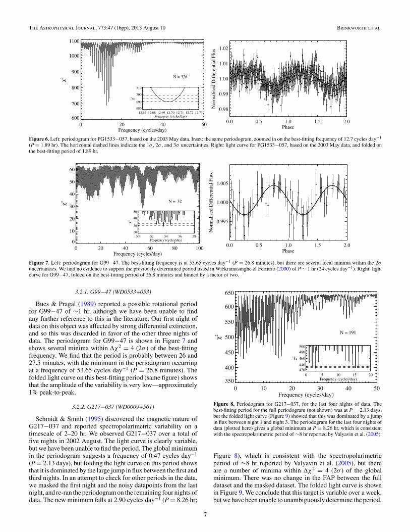
Figure 6. Left: periodogram for PG1533−057, based on the 2003 May data. Inset: the same periodogram, zoomed in on the best-fitting frequency of 12.7 cycles day−1

(P = 1.89 hr). The horizontal dashed lines indicate the 1σ , 2σ , and 3σ uncertainties. Right: light curve for PG1533−057, based on the 2003 May data, and folded onthe best-fitting period of 1.89 hr.

50 52 54 56 58Frequency (cycles/day)

20

30

40

50

χ2

0 20 40 60 80 100Frequency (cycles/day)

0

10

20

30

40

50

60

χ2 N = 32

0.0 0.5 1.0 1.5 2.0Phase

0.995

1.000

1.005

Nor

mal

ised

Dif

fere

ntia

l Flu

x

Figure 7. Left: periodogram for G99−47. The best-fitting frequency is at 53.65 cycles day−1 (P = 26.8 minutes), but there are several local minima within the 2σ

uncertainties. We find no evidence to support the previously determined period listed in Wickramasinghe & Ferrario (2000) of P ∼ 1 hr (24 cycles day−1). Right: lightcurve for G99−47, folded on the best-fitting period of 26.8 minutes and binned by a factor of two.

3.2.1. G99−47 (WD0533+053)

Bues & Pragal (1989) reported a possible rotational periodfor G99−47 of ∼1 hr, although we have been unable to findany further reference to this in the literature. Our first night ofdata on this object was affected by strong differential extinction,and so this was discarded in favor of the other three nights ofdata. The periodogram for G99−47 is shown in Figure 7 andshows several minima within Δχ2 = 4 (2σ ) of the best-fittingfrequency. We find that the period is probably between 26 and27.5 minutes, with the minimum in the periodogram occurringat a frequency of 53.65 cycles day−1 (P = 26.8 minutes). Thefolded light curve on this best-fitting period (same figure) showsthat the amplitude of the variability is very low—approximately1% peak-to-peak.

3.2.2. G217−037 (WD0009+501)

Schmidt & Smith (1995) discovered the magnetic nature ofG217−037 and reported spectropolarimetric variability on atimescale of 2–20 hr. We observed G217−037 over a total offive nights in 2002 August. The light curve is clearly variable,but we have been unable to find the period. The global minimumin the periodogram suggests a frequency of 0.47 cycles day−1

(P = 2.13 days), but folding the light curve on this period showsthat it is dominated by the large jump in flux between the first andthird nights. In an attempt to check for other periods in the data,we masked the first night and the noisy datapoints from the lastnight, and re-ran the periodogram on the remaining four nights ofdata. The new minimum falls at 2.90 cycles day−1 (P = 8.26 hr;

0 5 10 15 20Frequency (cycles/day)

420440

460

480500

χ2

0 10 20 30 40 50Frequency (cycles/day)

350

400

450

500

550

600

650

χ2

N = 191

Figure 8. Periodogram for G217−037, for the last four nights of data. Thebest-fitting period for the full periodogram (not shown) was at P = 2.13 days,but the folded light curve (Figure 9) showed that this was dominated by a jumpin flux between night 1 and night 3. The periodogram for the last four nights ofdata (plotted here) gives a global minimum at P = 8.26 hr, which is consistentwith the spectropolarimetric period of ∼8 hr reported by Valyavin et al. (2005).

Figure 8), which is consistent with the spectropolarimetricperiod of ∼8 hr reported by Valyavin et al. (2005), but thereare a number of minima within Δχ2 = 4 (2σ ) of the globalminimum. There was no change in the FAP between the fulldataset and the masked dataset. The folded light curve is shownin Figure 9. We conclude that this target is variable over a week,but we have been unable to unambiguously determine the period.

7

The Astrophysical Journal, 773:47 (16pp), 2013 August 10 Brinkworth et al.

0.0 0.5 1.0 1.5 2.0Phase

0.98

0.99

1.00

1.01

1.02

Nor

mal

ised

Dif

fere

ntia

l Flu

x

0.0 0.5 1.0 1.5 2.0Phase

0.98

0.99

1.00

1.01

1.02

Nor

mal

ised

Dif

fere

ntia

l Flu

x

Figure 9. Left: the data for G217−037, taken over five nights, folded on the best-fitting period for all of the data of P = 2.13 days. The nights have been color-coded,with night 1 blue, night 2 green, night 3 black, night 4 red, and night 5 yellow. The period is dominated by the jump in flux between nights 1 and 3. Right: the lightcurve folded on the best period from just the last four nights (P = 8.26 hr). This is consistent with the spectropolarimetric period reported by Valyavin et al. (2005).

(A color version of this figure is available in the online journal.)

400 500 600 700 800HJD−52000 (days)

0.95

1.00

1.05

1.10

Nor

mal

ised

Dif

fere

ntia

l Flu

x

0 2 4 6 8 10Frequency (cycles/day)

360380400420440460

χ2

0 10 20 30 40 50Frequency (cycles/day)

0

500

1000

1500

χ2

N = 89

Figure 10. Left: the data for G227−28, showing a drop of ∼3% in the differential flux over the year. Right: the periodogram for G227−28 shows a significant globalminimum at 3.19 cycles day−1 (7.5 hr), but the folded light curves (Figure 11) do not support a short-term periodicity.

0.0 0.5 1.0 1.5 2.0Phase

0.96

0.98

1.00

1.02

1.04

1.06

1.08

1.10

Nor

mal

ised

Dif

fere

ntia

l Flu

x

0.0 0.5 1.0 1.5 2.0Phase

0.95

1.00

1.05

1.10

Nor

mal

ised

Dif

fere

ntia

l Flu

x

Figure 11. Left: all of the data on G227−28, folded on the best period of P = 7.5 hr. Data from the first epoch are in black, and from the second are shown in blue.Right: August data alone, folded on the best period for that dataset, of P = 1.31 days.

(A color version of this figure is available in the online journal.)

3.2.3. G227−28 (WD1820+609)

We find no evidence for variability in this object over shorttimescales, but find that there is a drop of 3% in the differentialphotometry over the year (Figure 10). We have been unable todetermine a period (Figure 11), so simply conclude that thistarget is probably varying over timescales of ∼ months–yearswith full amplitude of 3% or more. We are conducting follow-upobservations to confirm these long-term modulations.

3.2.4. G240−72 (WD1748+708)

Berdyugin & Pirola (1999) reported extremely slow variabil-ity in the polarization of this object over several decades, which

they interpret as a rotational period of �100 yr. We find no evi-dence for short-term variability in this star: the rms of the scatterin the light curve is lower than the rms of the scatter in the com-parisons. We do, however, see an increase in the differential fluxof ∼2.5% over the 10 months between 2002 August and 2003May (Figure 12), well above the rms level of the comparisons,and the χ2 of the best-fitting period is Δχ2 = 1382 better thanfor a constant fit. The periodogram is dominated by the scatterat short periods, so we have not included it here. We also ran aperiodogram on the August data alone to check for short-termperiodicity buried in the scatter. We found no significant min-ima below the Nyquist frequency, and the χ2 of a constant fit

8

The Astrophysical Journal, 773:47 (16pp), 2013 August 10 Brinkworth et al.

400 500 600 700 800HJD−52000 (days)

0.94

0.96

0.98

1.00

1.02

1.04

1.06N

orm

alis

ed D

iffe

rent

ial F

lux

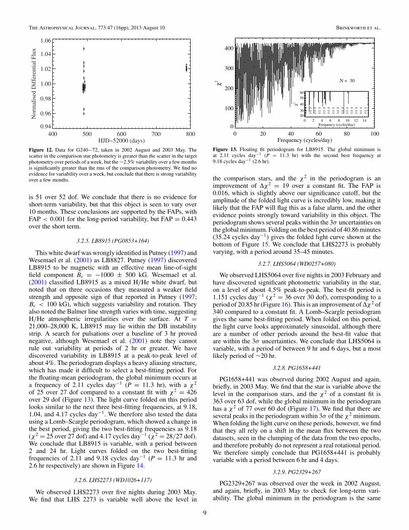
Figure 12. Data for G240−72, taken in 2002 August and 2003 May. Thescatter in the comparison star photometry is greater than the scatter in the targetphotometry over periods of a week, but the ∼2.5% variability over a few monthsis significantly greater than the rms of the comparison photometry. We find noevidence for variability over a week, but conclude that there is strong variabilityover a few months.

is 51 over 52 dof. We conclude that there is no evidence forshort-term variability, but that this object is seen to vary over10 months. These conclusions are supported by the FAPs, withFAP < 0.001 for the long-period variability, but FAP = 0.443over the short term.

3.2.5. LB8915 (PG0853+164)

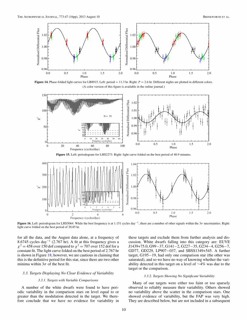
This white dwarf was wrongly identified in Putney (1997) andWesemael et al. (2001) as LB8827. Putney (1997) discoveredLB8915 to be magnetic with an effective mean line-of-sightfield component Be = −1000 ± 500 kG. Wesemael et al.(2001) classified LB8915 as a mixed H/He white dwarf, butnoted that on three occasions they measured a weaker fieldstrength and opposite sign of that reported in Putney (1997;Be < 100 kG), which suggests variability and rotation. Theyalso noted the Balmer line strength varies with time, suggestingH/He atmospheric irregularities over the surface. At T =21,000–28,000 K, LB8915 may lie within the DB instabilitystrip. A search for pulsations over a baseline of 3 hr provednegative, although Wesemael et al. (2001) note they cannotrule out variability at periods of 2 hr or greater. We havediscovered variability in LB8915 at a peak-to-peak level ofabout 4%. The periodogram displays a heavy aliasing structure,which has made it difficult to select a best-fitting period. Forthe floating-mean periodogram, the global minimum occurs ata frequency of 2.11 cycles day−1 (P = 11.3 hr), with a χ2

of 25 over 27 dof compared to a constant fit with χ2 = 426over 29 dof (Figure 13). The light curve folded on this periodlooks similar to the next three best-fitting frequencies, at 9.18,1.04, and 4.17 cycles day−1. We therefore also tested the datausing a Lomb–Scargle periodogram, which showed a change inthe best period, giving the two best-fitting frequencies as 9.18(χ2 = 25 over 27 dof) and 4.17 cycles day−1 (χ2 = 28/27 dof).We conclude that LB8915 is variable, with a period between2 and 24 hr. Light curves folded on the two best-fittingfrequencies of 2.11 and 9.18 cycles day−1 (P = 11.3 hr and2.6 hr respectively) are shown in Figure 14.

3.2.6. LHS2273 (WD1026+117)

We observed LHS2273 over five nights during 2003 May.We find that LHS 2273 is variable well above the level in

0 2 4 6 8 10 12 14Frequency (cycles/day)

2030

40

5060

χ2

0 20 40 60 80 100Frequency (cycles/day)

0

100

200

300

400

χ2 N = 30

Figure 13. Floating fit periodogram for LB8915. The global minimum isat 2.11 cycles day−1 (P = 11.3 hr) with the second best frequency at9.18 cycles day−1 (2.6 hr).

the comparison stars, and the χ2 in the periodogram is animprovement of Δχ2 = 19 over a constant fit. The FAP is0.016, which is slightly above our significance cutoff, but theamplitude of the folded light curve is incredibly low, making itlikely that the FAP will flag this as a false alarm, and the otherevidence points strongly toward variability in this object. Theperiodogram shows several peaks within the 3σ uncertainties onthe global minimum. Folding on the best period of 40.86 minutes(35.24 cycles day−1) gives the folded light curve shown at thebottom of Figure 15. We conclude that LHS2273 is probablyvarying, with a period around 35–45 minutes.

3.2.7. LHS5064 (WD0257+080)

We observed LHS5064 over five nights in 2003 February andhave discovered significant photometric variability in the star,on a level of about 4.5% peak-to-peak. The best-fit period is1.151 cycles day−1 (χ2 = 36 over 30 dof), corresponding to aperiod of 20.85 hr (Figure 16). This is an improvement of Δχ2 of340 compared to a constant fit. A Lomb–Scargle periodogramgives the same best-fitting period. When folded on this period,the light curve looks approximately sinusoidal, although thereare a number of other periods around the best-fit value thatare within the 3σ uncertainties. We conclude that LHS5064 isvariable, with a period of between 9 hr and 6 days, but a mostlikely period of ∼20 hr.

3.2.8. PG1658+441

PG1658+441 was observed during 2002 August and again,briefly, in 2003 May. We find that the star is variable above thelevel in the comparison stars, and the χ2 of a constant fit is363 over 63 dof, while the global minimum in the periodogramhas a χ2 of 77 over 60 dof (Figure 17). We find that there areseveral peaks in the periodogram within 3σ of the χ2 minimum.When folding the light curve on these periods, however, we findthat they all rely on a shift in the mean flux between the twodatasets, seen in the clumping of the data from the two epochs,and therefore probably do not represent a real rotational period.We therefore simply conclude that PG1658+441 is probablyvariable with a period between 6 hr and 4 days.

3.2.9. PG2329+267

PG2329+267 was observed over the week in 2002 August,and again, briefly, in 2003 May to check for long-term vari-ability. The global minimum in the periodogram is the same

9

The Astrophysical Journal, 773:47 (16pp), 2013 August 10 Brinkworth et al.

0.0 0.5 1.0 1.5 2.0Phase

0.96

0.98

1.00

1.02N

orm

alis

ed D

iffe

rent

ial F

lux

0.0 0.5 1.0 1.5 2.0Phase

0.96

0.98

1.00

1.02

Nor

mal

ised

Dif

fere

ntia

l Flu

x

Figure 14. Phase-folded light curves for LB8915. Left: period = 11.3 hr. Right: P = 2.6 hr. Different nights are plotted in different colors.

(A color version of this figure is available in the online journal.)

0 10 20 30 40 50 60Frequency (cycles/day)

80859095

100105110

χ2

0 20 40 60 80 100Frequency (cycles/day)

0

50

100

150

χ2

N = 35

0.0 0.5 1.0 1.5 2.0Phase

0.98

0.99

1.00

1.01

1.02

Nor

mal

ised

Dif

fere

ntia

l Flu

x

Figure 15. Left: periodogram for LHS2273. Right: light curve folded on the best period of 40.9 minutes.

0 1 2 3 4 5 6Frequency (cycles/day)

2040

60

80100

χ2

0 2 4 6Frequency (cycles/day)

0

100

200

300

400

χ2

0.0 0.5 1.0 1.5 2.0Phase

0.96

0.98

1.00

1.02

1.04

Nor

mal

ised

Dif

fere

ntia

l Flu

x

Figure 16. Left: periodogram for LHS5064. While the best frequency is at 1.151 cycles day−1, there are a number of other signals within the 3σ uncertainties. Right:light curve folded on the best period of 20.85 hr.

for all the data, and the August data alone, at a frequency of8.6745 cycles day−1 (2.767 hr). A fit at this frequency gives aχ2 = 458 over 150 dof compared to χ2 = 707 over 152 dof for aconstant fit. The light curve folded on the best period of 2.767 hris shown in Figure 18; however, we are cautious in claiming thatthis is the definitive period for this star, since there are two otherminima within 3σ of the best fit.

3.3. Targets Displaying No Clear Evidence of Variability

3.3.1. Targets with Variable Comparisons

A number of the white dwarfs were found to have peri-odic variability in the comparison stars on level equal to orgreater than the modulation detected in the target. We there-fore conclude that we have no evidence for variability in

these targets and exclude them from further analysis and dis-cussion. White dwarfs falling into this category are: EUVEJ1439+75.0, G99−37, G141−2, G227−35, G234−4, G256−7,GD77, GD229, LP907−037, and SBSS1349+545. A furthertarget, G195−19, had only one comparison star (the other wassaturated), and so we have no way of knowing whether the vari-ability detected in this target on a level of ∼4% was due to thetarget or the comparison.

3.3.2. Targets Showing No Significant Variability

Many of our targets were either too faint or too sparselyobserved to reliably measure their variability. Others showedno variability above the scatter in the comparison stars. Oneshowed evidence of variability, but the FAP was very high.They are described below, but are not included in a subsequent

10

The Astrophysical Journal, 773:47 (16pp), 2013 August 10 Brinkworth et al.

0 2 4 6 8 10Frequency (cycles/day)

6070

80

90100

χ2

0 20 40 60 80 100Frequency (cycles/day)

0

100

200

300

400

χ2 N = 64

0.0 0.5 1.0 1.5 2.0Phase

0.98

0.99

1.00

1.01

1.02

Nor

mal

ised

Dif

fere

ntia

l Flu

x

Figure 17. Left: periodogram for PG1658+441. Right: light curve for PG1658+441, folded on the best period from the periodogram. The shift in mean flux betweenthe two epochs makes it hard to determine whether this is a genuine rotational period, and so we simply conclude that the source is variable, with a possible periodbetween 6 hr and 4 days.

(A color version of this figure is available in the online journal.)

6 8 10 12 14Frequency (cycles/day)

440450460470480490500

χ2

0 20 40 60 80 100Frequency (cycles/day)

400

450

500

550

600

650

700

χ2 N = 153

0.0 0.5 1.0 1.5 2.0Phase

0.98

1.00

1.02

1.04

Nor

mal

ised

Dif

fere

ntia

l Flu

x

Figure 18. Left: periodograms for PG2329+267. The periodogram for all the data (shown) and that for just the August data (not shown) give the same global minimumat 8.6745 cycles day−1. Right: the data for PG2329+267, folded on the best period of 2.767 hr.

analysis. Some have been included in our long-term follow-upstudy to search for variability on timescales of months–years.

3.3.2.1. G158−45 (WD0011−134)

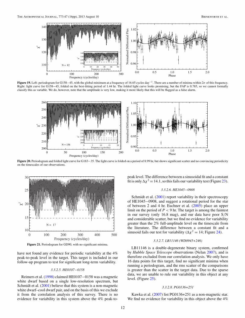
Putney (1997) reported polarimetric variations in G158−45,suggesting a rotational period of between 11 hr and a few days.We observed the system over six nights during the August run,and found tentative evidence for photometric variability in thestar with a period between 30 minutes and a few days and apeak-to-peak amplitude of ∼1%. The global minimum at P =1.44 hr has a χ2 of 112 over 79 dof, which is significantly betterthan a constant fit with χ2 of 142 over 81 dof. It should be notedthat G158−45 is at the faint end of our sample (15.9 mag),and so the uncertainties on the data points are relatively large(± ∼0.75%; Figure 19). Despite the evidence for variability inthis object, the FAP is very high, at 0.785, so we are unable toinclude G158−45 in the list of variable sources. This target isincluded in our follow-up study sample.

3.3.2.2. G183−35 (WD1814+248)

Putney (1997) reported possible rotation of this object witha period between 50 minutes and a few years. From ourphotometric data, taken over a week in 2002 August and afurther week in 2003 May, we find no evidence of rotation ontimescales of less than a year. A constant fit to the data givesa χ2 of 122 over 152 dof, compared to a χ2 minimum in theperiodogram of 101 over 149 dof (Figure 20), but, as these

numbers suggest, the uncertainties on the data points are toolarge for this to be meaningful. A light curve folded on theperiodogram global minimum shows that the data are flat overthe year. We conclude that G183−35 is not varying at the 4%peak-to-peak level on timescales of less than a year, and arefollowing up this object on longer timescales.

3.3.2.3. GD90 (WD0816+376)

Due to poor observing conditions, we only took 16 obser-vations of GD90 during the 2003 February run. While the dif-ference between a constant and sinusoidal fit formally suggestsvariability (Δχ2 = 23), there was no significant global min-imum in the periodogram (the minimum was at a period of7.7 minutes; Figure 21). We rule out variability at the 4% peak-to-peak level, and conclude that more data are required on thisobject.

3.3.2.4. Grw +70◦8247 (WD1900+70)

The polarization curves for this star have remained unchangedover 25 yr of observations, suggesting that this star is a very slowrotator, with a period of �100 yr. We took data over the week ofthe 2002 August run, plus one set during 2003 May to check forany long-term variations over the year. A constant fit to the datahas a χ2 of 472 over 148 dof, while the global minimum in theperiodogram at 0.248 cycles day−1 has χ2 = 318 over 146 dof(Figure 22). We note that the rms scatter in the comparisons isgreater than the scatter in the target flux and conclude that we

11

The Astrophysical Journal, 773:47 (16pp), 2013 August 10 Brinkworth et al.

0 10 20 30 40 50Frequency (cycles/day)

110

120

130

140

χ2

0 100 200 300Frequency (cycles/day)

110

120

130

140

χ2

N = 82

0.0 0.5 1.0 1.5 2.0Phase

0.96

0.98

1.00

1.02

Nor

mal

ised

Dif

fere

ntia

l Flu

x

Figure 19. Left: periodogram for G158−45, with the global minimum at a frequency of 16.65 cycles day−1. There are a number of minima within 2σ of this frequency.Right: light curve for G158−45, folded on the best-fitting period of 1.44 hr. The folded light curve looks promising, but the FAP is 0.785, so we cannot formallyclassify this as variable. We do, however, note that the amplitude is very low, making it more likely that this will be flagged as a false alarm.

0 5 10 15 20Frequency (cycles/day)

200210

220

230240

χ2

0 50 100 150 200Frequency (cycles/day)

200

210

220

230

240

250

260

χ2

N = 158

0.0 0.5 1.0 1.5 2.0Phase

0.90

0.95

1.00

1.05

1.10

Nor

mal

ised

Dif

fere

ntia

l Flu

x

Figure 20. Periodogram and folded light curve for G183−35. The light curve is folded on a period of 8.99 hr, but shows significant scatter and no convincing periodicityon the timescales of our observations.

0 100 200 300 400 500Frequency (cycles/day)

10

15

20

25

30

χ2

N = 17

Figure 21. Periodogram for GD90, with no significant minima.

have not found any evidence for periodic variability at the 4%peak-to-peak level in the target. This target is included in ourfollow-up program to test for significant long-term variability.

3.3.2.5. HE0107−0158

Reimers et al. (1998) claimed HE0107−0158 was a magneticwhite dwarf based on a single low-resolution spectrum, butSchmidt et al. (2001) believe that this system is a non-magneticwhite dwarf–cool dwarf pair, and on the basis of this we excludeit from the correlation analysis of this survey. There is noevidence for variability in this system above the 4% peak-to-

peak level. The difference between a sinusoidal fit and a constantfit is only Δχ2 = 14.1, so this fails our variability test (Figure 23).

3.3.2.6. HE1045−0908

Schmidt et al. (2001) report variability in their spectroscopyof HE1045−0908, and suggest a rotational period for the starof between 2 and 4 hr. Euchner et al. (2005) place an upperlimit on the period of P < 9 hr. The target is among the faintestin our survey (only 16.8 mag), and our data have poor S/Nand considerable scatter, but we find no evidence for variabilitygreater than the 2% full-amplitude level on the timescale fromthe literature. The difference between a constant fit and asinusoid fails our test for variability (Δχ2 = 14; Figure 24).

3.3.2.7. LB11146 (WD0945+246)

LB11146 is a double-degenerate binary system, confirmedby Hubble Space Telescope observations (Nelan 2007), and istherefore excluded from our correlation analysis. We only have16 data points for this target, find no significant minima whenrunning a periodogram, and the rms scatter of the comparisonsis greater than the scatter in the target data. Due to the sparsedata, we are unable to rule out variability in this object at anylevel. (Figure 25).

3.3.2.8. PG0136+251

Kawka et al. (2007) list PG0136+251 as a non-magnetic star.We find no evidence for variability in this object above the 4%

12

The Astrophysical Journal, 773:47 (16pp), 2013 August 10 Brinkworth et al.

0.0 0.5 1.0 1.5 2.0 2.5 3.0Frequency (cycles/day)

320340

360

380400

χ2

0 20 40 60 80 100Frequency (cycles/day)

300

350

400

450

500

550

χ2

N = 150

0.0 0.5 1.0 1.5 2.0Phase

0.98

0.99

1.00

1.01

1.02

1.03

1.04

Nor

mal

ised

Dif

fere

ntia

l Flu

x

Figure 22. Periodogram and folded light curve for Grw+70◦8247. The light curve is folded on a period of 4.03 days, but shows significant scatter and no convincingperiodicity on the timescales of our observations.

0 50 100 150 200Frequency (cycles/day)

35

40

45

50

χ2

N = 55

Figure 23. Periodogram for HE0107−0158, with no significant minima.

0 20 40 60 80 100 120 140Frequency (cycles/day)

25

30

35

40

45

χ2

N = 42

Figure 24. Periodogram for HE1045−0908, with no significant minima.

level. The global minimum in the periodogram is insignificantwhen compared to a constant fit, with Δχ2 = 12 (Figure 26).

4. DISCUSSION

Of our 33 targets, 2 are believed to be binary systems(HE0107−0158, EUVE J1439+75.0), and 1 (PG0136+251) isbelieved to be non-magnetic (and indeed found here to be non-variable), and they are therefore excluded from further analysis.Of the remaining 30 isolated magnetic white dwarfs, 5 are

0 20 40 60 80 100Frequency (cycles/day)

0

10

20

30

40

50

60

χ2N = 13

Figure 25. Periodogram for LB11146, with no significant minima.

0 20 40 60 80 100 120 140Frequency (cycles/day)

35

40

45

50

χ2

N = 60

Figure 26. Periodogram for PG0136+251, with no significant minima.

variable with reliably derived rotation periods, and a further9 are seen to vary during our study, but we were unable todetermine the period.

There is no evidence for variability in the remaining16 objects: 9 had variable comparison stars, 5 require moredata, and 2 were not seen to vary above the scatter in the com-parisons. The period distribution for the variable magnetic whitedwarfs in our sample can be seen in Figure 1.

13

The Astrophysical Journal, 773:47 (16pp), 2013 August 10 Brinkworth et al.

Figure 27. Plot of field strength vs. measured period for our variable whitedwarf sample. Also included are WD1953−011 and GD356, from Brinkworthet al. (2004, 2005). The shape of the plotting symbols describes the whitedwarf composition—DA white dwarfs are plotted as circles, DB white dwarfsas upright triangles, while targets that have been reported as both DA and DB areplotted as upside-down triangles. We find no correlation between field strengthand spin period in our sample.

Figure 28. Plot of effective temperature vs. measured period for our variablewhite dwarf sample. Also included are WD1953−011 and GD356, fromBrinkworth et al. (2004, 2005). The shape of the plotting symbols describes thewhite dwarf composition—DA white dwarfs are plotted as circles, DB whitedwarfs as upright triangles, while targets that have been reported as both DAand DB are plotted as upside-down triangles. We find no correlation betweeneffective temperature and spin period in our sample.

4.1. Correlations between Rotation Period andOther White Dwarf Parameters

We searched for correlations between the period of variability(which we interpret as the spin period, for reasons describedearlier) and the field strength, mass, temperature, and age of thestars. For the sources without a well-defined period, we simplyused the best estimate from the periodogram, with the error barscovering the possible range of periods over 3σ (Figures 27–30).We find no correlation between spin period and any other testedparameter. Wickramasinghe & Ferrario (2000) found a positivecorrelation between period and magnetic field strength at shorterperiods, and Ferrario & Wickramasinghe (2005) found a similarresult when including the slow rotators, but we find no evidencefor this in our data.

Interestingly, we have discovered variability in eight targetswith both low temperatures (T < 12,000 K) and low magnetic

Figure 29. Plot of mass vs. measured period for our variable white dwarfsample. Also included are WD1953−011 and GD356, from Brinkworth et al.(2004, 2005). The shape of the plotting symbols describes the white dwarfcomposition—DA white dwarfs are plotted as circles, DB white dwarfs asupright triangles, while targets that have been reported as both DA and DB areplotted as upside-down triangles. We find no correlation between mass and spinperiod in our sample.

Figure 30. Plot of age vs. measured period for our variable white dwarfsample. Also included are WD1953−011 and GD356, from Brinkworth et al.(2004, 2005). The shape of the plotting symbols describes the white dwarfcomposition—DA white dwarfs are plotted as circles, DB white dwarfs asupright triangles, while targets that have been reported as both DA and DB areplotted as upside-down triangles. We find no correlation between white dwarfage and spin period in our sample.

field strengths (B < 20 MG). The most likely explanationfor this is the presence of starspots on their surfaces, asseen in WD1953−011 (Brinkworth et al. 2005) and GD356(Brinkworth et al. 2004). This is possibly due to the partially con-vective atmospheres of these low-temperature targets. Follow-up polarimetry of these eight targets could confirm the presenceof starspots.

More surprisingly, we also find variability in two targetswith low magnetic field strength, but high temperatures (T >20,000 K): LB8915 and PG1658+441. LB8915 is a DBA whitedwarf, i.e., it has a helium dominated atmosphere with weakhydrogen lines in its optical spectrum. At Teff ∼ 20,000 K, itmay still have a partially convective atmosphere, and so may stillbe able to form starspots despite its high temperature. Combinedwith data from Wesemael et al. (2001) showing polarimetric

14

The Astrophysical Journal, 773:47 (16pp), 2013 August 10 Brinkworth et al.

variability, it seems likely that the variability in LB8915 is dueto magnetic field effects, most likely a starspot. PG1658+441,on the other hand, is a hydrogen-rich magnetic DA white dwarfwith a field strength (3.5 MG) too low to cause magneticdichroism and, at Teff = 30,500 K, a fully radiative atmospherethat cannot form starspots. Infrared observations at Two MicronAll Sky Survey and Spitzer Space Telescope wavelengths findno IR excess indicative of a companion (Hansen et al. 2006),with an upper limit on an unresolved companion of 2 Jupitermasses (Farihi et al. 2008). The source of variability in PG1658therefore remains a mystery.

5. CONCLUSIONS

Of 30 isolated magnetic white dwarfs, we find that 9 wereuntestable due to varying comparison stars. Of the remaining 21,14 show evidence for variability (67%), and 7 show no evidenceof variability and would benefit from further observations. The9 discarded for having variable comparison stars would alsobenefit from repeat observations using a different field of view.Long-term follow-up of a number of the targets is currentlyunderway.

We find no evidence for any correlation between spin periodand any other white dwarf parameters, but note that few ofour targets have well-defined periods. Our long-term follow-upshould provide better constraints.

The authors would like to thank the referee for the carefulhelpful comments that greatly improved this paper.

Matt Burleigh acknowledges the support of a PPARC/STFCAdvanced Fellowship during the course of this project. TomMarsh acknowledges support from STFC during the course ofthis research.

The Jacobus Kapteyn Telescope is operated on the island of LaPalma by the Isaac Newton Group in the Spanish Observatoriodel Roque de los Muchachos of the Instituto de Astrofsica deCanarias. This research has made use of the SIMBAD database,operated at CDS, Strasbourg, France. This research has made useof NASA’s Astrophysics Data System Bibliographic Services.

REFERENCES

Angel, J. R. P. 1978, ARA&A, 16, 487Angel, J. R. P., Carswell, R. F., Beaver, E. A., Harms, R., & Strittmatter, P. A.

1974, ApJL, 194, L47Barstow, M. A., Jordan, S., O’Donoghue, D., et al. 1995, MNRAS, 277, 971Berdyugin, A. V., & Pirola, V. 1999, A&A, 352, 619Berger, L., Koester, D., Napiwotzki, R., Reid, I. N., & Zuckerman, B.

2005, A&A, 444, 565Bergeron, P., Leggett, S. K., & Ruiz, M. T. 2001, ApJS, 133, 413Bergeron, P., Ruiz, M. T., & Leggett, S. K. 1997, ApJS, 108, 339Brinkworth, C. S., Burleigh, M. R., Wynn, G. A., & Marsh, T. R. 2004, MNRAS,

384, L33Brinkworth, C. S., Marsh, T. R., Morales-Rueda, L., et al. 2005, MNRAS,

357, 333Bues, I., & Pragal, M. 1989, LNP, 328, 329Burleigh, M. R., Jordan, S., & Schweizer, W. 1999, ApJL, 510, L37Cohen, M. H., Putney, A., & Goodrich, R. W. 1993, ApJL, 405, L67Cumming, A., Marcy, G. W., & Butler, R. P. 1999, ApJ, 526, 890Dhillon, V. S., Marsh, T. R., Stevenson, M. J., et al. 2007, MNRAS, 378, 825Dufour, P., Bergeron, P., & Fontaine, G. 2005, ApJ, 627, 404Dupuis, J., Vennes, S., & Chayer, P. 2002, ApJ, 580, 1091Euchner, F., Jordan, S., Beuermann, K., Reinsch, K., & Gansicke, B. T.

2006, A&A, 451, 671Euchner, F., Reinsch, K., Jordan, S., Beuermann, K., & Gansicke, B. T.

2005, A&A, 442, 651Farihi, J., Becklin, E. E., & Zuckerman, B. 2008, ApJ, 681, 1470Ferrario, L., Vennes, S., Wickramasinghe, D. T., Bailey, J., & Christian, D. J.

1997, MNRAS, 292, 205

Ferrario, L., & Wickramasinghe, D. T. 2005, MNRAS, 356, 615Friedrich, S., Oestreicher, R., & Schweizer, W. 1996, A&A, 309, 227Garcia-Berro, E., Loren-Aguilar, P., Aznar-Siguan, G., et al. 2012, ApJ, 749, 25Glenn, J., Liebert, J., & Schmidt, G. D. 1994, PASP, 106, 722Green, R. F., & Liebert, J. 1981, PASP, 93, 105Greenstein, J. L. 1986, ApJ, 304, 334Greenstein, J. L., & McCarthy, J. K. 1985, ApJ, 289, 732Greenstein, J. L., Oke, J. B., Richstone, D., Altena, W. F. V., & Steppe, H.

1977, ApJL, 218, L21Guseinov, O. H., Novruzova, H. I., & Rustamov, Yu. S. 1983a, Ap&SS, 97, 305Guseinov, O. H., Novruzova, H. I., & Rustamov, Yu. S. 1983b, Ap&SS, 96, 1Hansen, B. M. S., Kulkarni, S., & Wiktorowicz, S. 2006, AJ, 131, 1106Hermes, J. J., Montgomery, M. H., Winget, D. E., et al. 2012, ApJL, 750, L28Holberg, J. B., Sion, E. M., Oswalt, T., et al. 2008, AJ, 135, 1225Jordan, S., Aznar Cuadrado, R., Napiwotzki, R., Schmid, H. M., & Solanki,

S. K. 2007, A&A, 462, 1097Jordan, S., Schmelcher, P., & Becken, W. 2001, A&A, 376, 614Karl, C. A., Napiwotzki, R., Heber, U., et al. 2005, A&A, 434, 637Kawaler, S. D. 2004, in IAU Symp. 215, Stellar Rotation, ed. A. Maeder & P.

Eenens (San Francisco, CA: ASP), 561Kawka, A., & Vennes, S. 2004, in IAU Symp. 224, The A-Star Puzzle, ed. J.

Zverko, J. Ziznovsky, S. J. Adelman, & W. W. Weiss (Cambridge: CambridgeUniv. Press), 879

Kawka, A., Vennes, S., Schmidt, G. D., Wickramasinghe, D. T., & Koch, R.2007, ApJ, 654, 499

Kepler, S. O., Giovannini, O., Wood, M. A., et al. 1995, ApJ, 447, 874Kepler, S. O., Pelisoli, I., Jordan, S., et al. 2013, MNRAS, 429, 2934King, A. R., Pringle, J. E., & Wickramasinghe, D. T. 2001, MNRAS, 320, L45Kleinman, S. J., Kepler, S. O., Koester, D., et al. 2013, ApJS, 204, 5Koester, D., Dreizler, S., Weidermann, V., & Allard, N. F. 1998, A&A, 338, 612Kulebi, B., Jordan, S., Euchner, F., Gansicke, B. T., & Hirsch, H. 2009, A&A,

506, 1341Liebert, J. 1976, PASP, 88, 490Liebert, J., Bergeron, P., & Holberg, J. B. 2003, AJ, 125, 348Liebert, J., Bergeron, P., Schmidt, G. D., & Saffer, R. A. 1993, ApJ, 418, 426Liebert, J., Schmidt, G. D., Green, R. F., Stockman, H. S., & McGraw, J. T.

1983, ApJ, 264, 262Liebert, J., Schmidt, G. D., Sion, E. M., et al. 1985, PASP, 97, 158Liebert, J., Smith, G. D., Lesser, M., et al. 1994, ApJ, 421, 733Liebert, J., Wickramsinghe, D. T., Schmidt, G. D., et al. 2005, AJ, 129, 2376Limoges, M.-M., & Bergeron, P. 2010, ApJ, 714, 1037Lomb, N. R. 1976, Ap&SS, 39, 447Maxted, P. F. L., Ferrario, L., Marsh, T. R., & Wickramasinghe, D. T.

2000, MNRAS, 315, L41Morales-Rueda, L., Maxted, P. F. L., Marsh, T. R., North, R. C., & Heber, U.

2003, MNRAS, 338, 752Moran, C., Marsh, T. R., & Dhillon, V. S. 1998, MNRAS, 299, 218Mukadam, A. S., Montgomery, M. H., Kim, A., et al. 2006, ApJ, 640, 956Nelan, E. P. 2007, AJ, 134, 1934Nordhaus, J., Wellons, S., Spiegel, D. S., Metzger, B. D., & Blackman, E. G.

2011, PNAS, 108, 3135Putney, A. 1995, ApJL, 451, L67Putney, A. 1997, ApJS, 112, 527Putney, A., & Jordan, S. 1995, ApJ, 449, 863Reimers, D., Jordan, S., Beckmann, V., Christlieb, N., & Wisotzki, L. 1998,

A&A, 337, L13Reimers, D., Jordan, S., Koehler, T., & Wisotzki, L. 1994, A&A, 285, 995Reimers, D., Jordan, S., Koester, D., et al. 1996, A&A, 311, 572Scargle, J. D. 1982, ApJ, 263, 835Schmidt, G. D., Allen, R. G., Smith, P. S., & Liebert, J. 1996, ApJ, 463, 320Schmidt, G. D., Bergeron, P., Liebert, J., & Saffer, R. A. 1992a, ApJ, 394, 693Schmidt, G. D., Harris, H. C., Leibert, J., et al. 2003, ApJ, 595, 1101Schmidt, G. D., Liebert, J., & Smith, P. S. 1998, ApJ, 116, 451Schmidt, G. D., & Norsworthy, J. E. 1991, ApJ, 366, 270Schmidt, G. D., & Smith, P. S. 1995, ApJ, 448, 305Schmidt, G. D., Stockman, H. S., & Smith, P. S. 1992b, ApJL, 398, L57Schmidt, G. D., Vennes, S., Wickramasinghe, D. T., & Ferrario, L.

2001, MNRAS, 328, 203Schmidt, G. D., West, S. C., Liebert, J., Greeen, R. F., & Stockman, H. S.

1986, ApJ, 309, 218Sion, E. H., Holberg, J. B., Oswalt, T. D., McCook, G. P., & Wasatonic, R.

2009, AJ, 138, 1681Spruit, H. C. 1998, A&A, 333, 603Tout, C. A., Wickramasinghe, D. T., Liebert, J., Ferrario, L., & Pringle, J. E.

2008, MNRAS, 387, 897Valyavin, G., Antonyuk, K., Plachinda, S., et al. 2011, ApJ, 734, 17Valyavin, G., Bagnulo, S., Monin, D., et al. 2005, A&A, 439, 1099

15

The Astrophysical Journal, 773:47 (16pp), 2013 August 10 Brinkworth et al.

Vanlandingham, K. M., Schmidt, G. D., Eisenstein, D. J., et al. 2005, AJ,130, 734

Vennes, S., Ferrario, L., & Wickramasinghe, D. T. 1999, MNRAS,302, L49

Vennes, S., Schmidt, G. D., Ferrario, L., et al. 2003, ApJ, 593, 1040Wesemael, F., Liebert, J., Schmidt, G. D., et al. 2001, ApJ, 554, 1118Wickramasinghe, D. T., & Cropper, M. 1988, MNRAS, 235, 1451

Wickramasinghe, D. T., & Ferrario, L. 1988, ApJ, 327, 222Wickramasinghe, D. T., & Ferrario, L. 2000, PASP, 112, 873Wickramasinghe, D. T., & Ferrario, L. 2005, MNRAS, 356, 1576Wickramasinghe, D. T., & Martin, B. 1979, MNRAS, 188, 165Wickramasinghe, D. T., Schmidt, G., Ferrario, L., & Vennes, S. 2002, MNRAS,

332, 29Winget, D. E., & Kepler, S. O. 2008, ARA&A, 46, 157

16