Measuring the quality of life in city of Indianapolis by

Dow

nloa

ded

By: [

Wen

g, Q

.] At

: 21:

10 2

8 M

arch

200

7

Measuring the quality of life in city of Indianapolis by integration ofremote sensing and census data

G. LI and Q. WENG*

Department of Geography, Geology, and Anthropology, Indiana State University, Terre

Haute, IN 47809, USA

(Received 27 May 2005; in final form 31 March 2006 )

This paper develops a methodology for integration of remote sensing and census

data within a GIS framework to assess the quality of life in Indianapolis, Indiana,

United States. Environmental variables, i.e. greenness, impervious surface and

temperature, were derived from a Landsat ETM + image. Socio-economic

variables, including population density, income, poverty, employment rate,

education level and house characteristics from US census 2000, were integrated

with the environmental variables at the block group level to derive indicators of

quality of life. Pearson’s correlation was computed to analyse the relationships

among the variables. Further, factor analysis was conducted to extract unique

information from the combined dataset. Three factors were identified and

interpreted as material welfare, environmental conditions and crowdedness

respectively. Each factor was viewed as a unique aspect of the quality of life. A

synthetic index of the urban quality of life was created and mapped based on

weighted factor scores of the three factors. Finally, regression models were built

to estimate the quality of life in the city of Indianapolis based on selected

environmental and socioeconomic variables.

Keywords: Urban quality of life; Remote sensing; Census; Data integration;

Indianapolis

1. Introduction

The study on the quality of life (QOL) in the cities of both developing and developed

countries is gaining interest from a variety of disciplines such as planning,

geography, sociology, economics, psychology, political science, behavioural

medicine, marketing and management (Andrew 1999, Foo 2001), and is becoming

an important tool for policy evaluation, rating of places, urban planning and

management. American economists Samuel Ordway (Ordway 1953) and Fairfield

Osborn (Osborn 1954) were among the earliest people to use this term to address

their concern over ecological dangers of unlimited economic growth. At present,

there is great deal of ambiguity and controversy on the concept of QOL, its elements

and indicators. Various concepts concerning QOL can be found in the literature,

such as urban environmental quality, livability, quality of place, residential-

perception and satisfaction and sustainability. Kamp et al. (2003) reviewed some

definitions about livability, QOL, environmental quality and sustainability, and

pointed out that there was neither comprehensive conceptual framework in relation

*Corresponding author. Email: [email protected]

International Journal of Remote Sensing

Vol. 28, No. 2, 20 January 2007, 249–267

International Journal of Remote SensingISSN 0143-1161 print/ISSN 1366-5901 online # 2007 Taylor & Francis

http://www.tandf.co.uk/journalsDOI: 10.1080/01431160600735624

Dow

nloa

ded

By: [

Wen

g, Q

.] At

: 21:

10 2

8 M

arch

200

7

to urban quality of life and human wellbeing developed, nor any agreed-on indicator

system to evaluate the physical, spatial and social aspects of urban quality owing to

the fact that a broad range of disciplines addressed different aspects of urban quality

of life based on different notions and theories. Bonaiuto et al. (2003) studied the

relationship between inhabitants and their neighbourhoods of residence in the urban

environment of Rome from the environmental psychological view, and proposed

two distinctive instruments. These instruments consisted of 11 scales for measuring

perceived environmental qualities of the urban neighbourhoods, with one scale

measuring neighbourhood attachment. This new version of perceived residential

environment quality and neighbourhood attachment largely improved internal

consistency with respect to earlier studies. Pacione (2003) addressed urban

environmental quality and human wellbeing from a social geographical perspective,

and presented a five-dimensional model for study of the quality of life, and

examined the major theoretical and methodological issues confronting quality of life

research. Although no consensus has been reached on the definition of the QOL,

most researchers would agree that QOL is a multidimensional construct,

encompassing aspects of psychological, economic, social and physical wellbeing.

Two approaches have been taken to identify QOL indicators: societal and personal

(Friedman 1997). Societal indicators are often used to study QOL in particular

societies or locations, such as communities, cities or nations. The data collected for

studies of the QOL in societies vary considerably depending upon research scales

and emphases. Smith (1973) suggested that data need to be collected in six broad

categories, including: (i) income, wealth and employment; (ii) the environment; (iii)

health; (iv) education; (v) social disorganization (crime, alcoholism, drug addiction);

and (iv) alienation and political participation. Personal indicators are often used to

determine resource allocation to improve health care, to assess the effects of

treatments and to help fulfill aspiration. Either societal indicators or personal

indicators can be measured objectively and subjectively.

In order to assess their effectiveness quantitatively, numerical measures called

social indicators have been constructed by Census Bureau, and used to monitor

trends in societal status, values and people’s QOL (Andrews and Whitney 1976).

Most previous work on urban QOL assessment used only socioeconomic variables

from census data, or socioeconomic data in conjunction with environment variables

derived from aerial photography. For example, Green (1957) employed aerial

photography to extract physical variables including housing density, number of

single family houses, land uses adjacent to and within residential area, and distance

of residential to central business district. Green then combined these data with

socioeconomic data such as education, crime rate and rental rates to rank each

residential area in Birmingham, Alabama, in terms of ‘residential desirability’. At

the meantime, poverty, as an aspect of QOL, has also been studied based on housing

density and other indicators derived from aerial photography by Mumbower and

Donoghue (1967) and Metivier and McCoy (1971). Bederman and Hartshorn (1984)

ranked QOL based on weighted socioeconomic variables extracted from census at

the county level for State of Georgia.

The advances of remote sensing and geographic information systems (GIS)

technologies make QOL research possible to be conducted based on digital remotely

sensed imagery and to incorporate digital imagery with census data. Weber and

Hirsch (1992) developed urban QOL indices by combining remotely sensed SPOT

data with census data for Stasbourg, France. It was found that there were some

250 G. Li and Q. Weng

Dow

nloa

ded

By: [

Wen

g, Q

.] At

: 21:

10 2

8 M

arch

200

7

strong correlations between census and remotely sensed data, mostly with housing

related data. Three urban QOL indices were developed based on the mixed data, and

were interpreted as housing, attractivity, and repulsion indices. Each of these indices

described only one aspect of QOL, but could not give a whole picture of QOL for a

specific unit. Lo and Faber (1997) created a QOL map for Athens-Clarke County,

Georgia, by combining environmental factors, including land use/cover, surface

temperature, and vegetation index derived from Landsat Thematic Mapper (TM),

with census variables, including population density, per capita income, median

home value, and percentage of college graduates using both principal component

analysis and GIS overlay methods. However, the first principal component, which

the authors interpreted as ‘the greenness of environment’, explained only 54.2% of

the total variance. Therefore, the measure of QOL based on the first principal

component was not complete, because it did not incorporate the second principal

component of ‘personal traits’ or higher order of components. Lo and Faber also

then ranked each variable based on its contribution to the QOL, and summed up the

ranks. Owing to the high correlation among these variables, the GIS method was

not able to remove redundant information.

This study focuses on the development of a methodology for integrating Landsat

Enhanced Thematic Mapper Plus (ETM + ) with Census 2000 in a GIS framework,

and applies the methodology to assess the quality of life in city of Indianapolis,

Indiana. Vegetation fraction, impervious surface fraction and land surface

temperature are derived from Landsat ETM + image as environmental indicators,

while income, education level, unemployment rate, poverty, house characteristics,

crowdedness, and other variables are extracted from the Census as socioeconomic

indicators. These two types of data are integrated in a GIS environment for further

analyses. To overcome the shortcomings of previous studies, a factor analysis is

conducted to reduce data dimensions. A QOL index is computed and mapped based

on factor weights. Moreover, a series of estimation models are developed based on

environmental and socioeconomic variables to predict QOL in the city.

2. Integration of remote sensing and GIS for urban analysis

The integration of remote sensing and GIS technologies has been widely applied and

been recognized as an effective tool in urban analysis and modelling (Ehlers et al.

1990, Treitz et al. 1992, Harris and Ventura 1995, Weng 2002). Remote sensing

collects multispectral, multiresolution and multitemporal data, and turns them into

information valuable for understanding and monitoring urban land processes and

for extracting urban environmental variables. GIS technology provides a flexible

environment for entering, analyzing, and displaying digital data from various

sources necessary for urban feature identification, change detection and database

development (Weng 2001).

Remotely sensed imagery and census data are two essential data sources for urban

analyses. Remote sensing data effectively record the physical properties of the

environment, provide large quantities of timely and accurate spatial information,

and are widely used in mapping and monitoring changes in land cover and land use

(Welch 1982, Forster 1985, Pathan et al. 1993, Weng 2002). Census data offer a wide

range of demographic and socio-economic information, and are used in racial and

ethnic diversity research (Frey 2001), urban planning and management. The

advance in GIS technology provides an effective environment for spatial analysis of

remotely sensed data and other sources of spatial data (Burrough 1986, Donnay

Measuring the quality of life in the city of Indianapolis 251

Dow

nloa

ded

By: [

Wen

g, Q

.] At

: 21:

10 2

8 M

arch

200

7

et al. 2001). Integration of remote sensing imagery and GIS (including census) data

have received widespread attention in recent years.

Wilkinson (1996) summarized three main ways in which remote sensing and GIS

technologies can be combined to enhance each other.

(1) Remote sensing is used as a tool for gathering data for use in GIS.

(2) GIS data are used as ancillary information to improve the products derived

from remote sensing.

(3) Remote sensing and GIS are used together for modeling and analysis.

Since census data collected within spatial units can be stored as GIS attributes, the

combination of census and remote sensing data through GIS can be envisaged in the

aforementioned three ways. Each of these ways has been related to urban analyses.

First, remote sensing imageries have been used in extracting and updating

transportation network (Lacoste et al., 2002, Harvey et al. 2004, Song and Civco

2004, Doucette et al. 2004, Kim et al. 2004), providing land use and land cover data(Haack et al. 1987, Ehlers et al. 1990, Treitz et al. 1992) and detecting urban

expansion (Yeh and Li 1997, Weng 2002, Cheng and Masser 2003). Second, census

data have been used to improve image classification in urban areas (Harris and

Ventura 1995, Mesev 1998). Finally, the integration of remote sensing and census

data has been applied to estimate population and residential density (Langford et al.

1991, Lo 1995, Sutton 1997, Yuan et al. 1997, Harris and Longley 2000, Martin et

al. 2000, Harvey 2000, 2002, Qiu et al. 2003, Li and Weng 2005). In addition,

integration of remote sensing with census data has also been used in detectingpoverty pocket (Hall et al. 2001), identifying housing sites for low-incomers

(Thomson 2000), and assessing urban quality of life (Weber and Hirsch 1992, Lo

and Faber 1997). So far, most of the works in the integration of remote sensing and

GIS were implemented by converting vector GIS data (including census data) into

raster format because of the similarity of remote sensing and raster GIS data

models. Only in recent years has the improvement of image analysis systems allowed

extraction of image data based on GIS polygons.

3. Study area

Marion County (Indianapolis), Indiana, USA (figure 1) has been chosen as the study

area. It is the core part of Indianapolis metropolitan area, and has the highest

concentration of major empoyers in manufacturing, professional, technical and

educational services in the state. With its moderate climate, rich history, excellent

education, social services, arts, leisure and recreation, Indianapolis was named one

of America’s Best Places to Live and Work (Employment Review’s August 1996).According to the 2000 census results, there are 658 block groups, 860 454 people,

and total 387 183 housing units. In 1999, unemployment rate is 3.7%, and 8.7%

families are under the US poverty level. Diversities in income, education level,

environment and other socioeconomic conditions within the city cause significant

differences in the QOL.

4. Dataset and methodology

4.1 Dataset

There are two primary data sources: Census 2000 and Landsat ETM + . The census

2000 data from the US Census Bureau used in this study include tabular data stored


Dow

nloa

ded

By: [

Wen

g, Q

.] At

: 21:

10 2

8 M

arch

200

7

in summary file 1 and summary file 3, which contain information about population,

housing, income and education etc. and spatial data, called topologically integrated

geographic encoding and referencing (TIGER), which contains data representing

the position and boundaries of legal and statistical entities. These two types of dataare linked together by census geographical entity codes. The US census has a

hierarchical structure composed of ten basic levels: USA, region, division, state,

county, county subdivision, place, census tract, block group and block. The block

group level was selected in this study.

Landsat 7 ETM + image (Row/Path: 32/21) dated on June 22, 2000 was used in

this research. Atmospheric conditions were clear at the time of image acquisition,

and the image was acquired through the United States Geological Survey (USGS)Earth Resource Observation Systems Data Center, which had corrected the

radiometric and geometrical distortions of the images to a quality level of 1G before

delivery. Two types of data were co-registered to Universal Tranverse Mercator

(UTM) system.

4.2 Methodology

Figure 2 gives the procedures of developing QOL index and predictive model. The

detailed descriptions of analytical procedures are given below.

4.2.1 Extraction of socioeconomic variables from census data. Selection of socio-

economic variables is based on the commonly used variables in previous studies

(Smith 1973, Weber and Hirsch 1992, Lo and Faber 1997). These variables include

population density, housing density, median family income, median household

income, per capita income, median house value, median number of rooms,percentage of college above graduates, unemployment rate and percentage of

families under poverty level. Initially, a total of 26 variables were extracted from

Figure 1. Study area: Marion County, Indiana, USA.


Dow

nloa

ded

By: [

Wen

g, Q

.] At

: 21:

10 2

8 M

arch

200

7

Census 2000 summary file 1 and file 3. A series of process was performed to obtain

the variables selected. TIGER shape file of block group was downloaded from the

internet. The socioeconomic variables were then integrated with TIGER shape file

using geographic entity codes as attributes of the shape file.

4.2.2 Extraction of environment variables. Previous studies show that vegetation

greenness and urban land use within given districts are important indicators of

quality of life, with high greenness and low percentage of urban use being of

higher quality. Greenness relates to vegetation, and can be measured using

vegetation indices such as NDVI (normalized difference vegetation index).

However, NDVI values are affected by many other external factors such as view

angle, soil background, seasons and differences in row direction and spacing in

agricultural field; therefore, it does not measure the amount of vegetation well

(Weng et al. 2004). Urban land use such as transportation, commercial and

industrial uses may be described as impervious surface, although impervious surface

is not limited to urban use. Impervious surface may also include some features in

residential areas, such as buildings and sidewalks. Vegetation abundance and

impervious surface are more accurate representation of urban morphological

composition. They can be obtained by using the technique of spectral mixture

analysis (SMA).

SMA is the technique used to solve the problem of mixed pixel in satellite imagery

with medium or coarse spatial resolution and to extract quantitative subpixel

information (Smith et al. 1990, Roberts et al. 1998, Mustard and Sunshine 1999). It

assumes that the reflectance spectrum by a sensor is the linear combination of the

spectra of the materials within the sensor’s field of view, frequently called

Figure 2. Flowchart showing the analytical procedures.


Dow

nloa

ded

By: [

Wen

g, Q

.] At

: 21:

10 2

8 M

arch

200

7

endmembers (Adams et al. 1995, Roberts et al. 1998). A detailed description of

SMA can be found (Roberts et al. 1998, Mustard and Sunshine 1999). Because of its

effectiveness in handling spectral mixture problems, SMA has been widely used in

estimation of vegetation cover (Smith et al. 1990, Asner and Lobell 2000, McGwire

et al. 2000, Small 2001), in land cover classification and change detection (Adams et

al. 1995, Roberts et al. 1998, Cochrane and Souza 1998, Aguiar et al. 1999, Lu et al.

2003), and in urban studies (Rashed et al. 2001, Phinn et al. 2002, Wu and Murray

2003, Lu and Weng 2004). In this study, three endmembers were initially identified

from the ETM + image based on high-resolution aerial photographs. The shade

endmember was identified from the areas of clear and deep water, while green

vegetation was selected from the areas of dense grass and cover crops. Different

types of impervious surfaces were selected from building roofs and highway

intersections. The radiances of these initial endmembers were compared with those

of the endmembers selected from the scatterplot of TM 3 and TM 4 and the

scatterplot of TM 4 and TM 5. The endmembers whose curves are similar but

located at the vertices of the scatterplot were finally used. A constrained least-

squares solution was used to decompose the six ETM + bands (1 through 5, and 7)

into three fraction images (vegetation, impervious surface and shade).

Temperature is an important factor affecting human comfort. High surface

temperature is regarded undesirable by most people; therefore, it can be used as an

indicator of environmental quality (Lo and Faber 1997, Nichol and Wong 2005).

Urban heat island is a common phenomenon in the cities where the urban area

shows a higher temperature than the rural area. Thermal infrared band of ETM +provides the source to extract surface temperatures. The procedure to extract land

surface temperatures involves three steps: (i) converting the digital number of

Landsat ETM + band 6 into spectral radiance; (ii) converting the spectral radiance

to at-satellite brightness temperature, which is also called blackbody temperature;

and (iii) converting the blackbody temperature to land surface temperature. A

detailed description of the procedures for extracting temperature images from

Landsat ETM + imagery can be found in Weng et al. (2004).

Since census data and ETM + data have different formats and spatial resolu-

tion, they need to be integrated. With the help of GIS function in ERDAS Imagine,

remote sensing data were aggregated at block group level, the mean values of

green vegetation, impervious surface and temperature were calculated for each

block group. All these data were then exported into SPSS software for further

analysis.

4.2.3 Factor analysis and development of QOL index. Factor analysis is a statistical

technique used to determine the number of underlying dimensions contained in a set

of observed variables. The underlying dimensions are referred to as factors. These

factors explain most of the variability among a large number of observed variables.

In factor analysis, the first factor explains most of the variance in the data, and each

successive factor explains less of the variance (Tabachnick and Fidell 1996). The

number of factors to be selected depends on the percentage of variance explained by

each factors. There are different factor extraction methods. The principal

component is one that is used in this study. Factors, whose eigenvalues greater

than 1 were extracted (Kaiser 1960)

Each factor can be viewed as one aspect of QOL. Therefore factor scores can be

used as a single index indicating the aspect with which the factor associates.

Synthetic QOL index is composite of different aspects. It is computed by the


Dow

nloa

ded

By: [

Wen

g, Q

.] At

: 21:

10 2

8 M

arch

200

7

following equation

QOL~Xn

1

FiWi ð1Þ

where n5the number of factors selected, Fi5factor i score, Wi5the percentage of

variance factor i explains. Finally, a QOL maps were created to show the geographic

patterns of QOL.

4.2.4 Regression analysis. Ideally, either single or synthetic QOL scores developed

based on factor analyses should be related to real QOL, and further the approach

can be validated. However, there are no such data available. Therefore, in this study

QOL scores created from factors were related to original indicators by developing

regression models. For single QOL, predictors were those that had large loadings on

the corresponding factor; for synthetic QOL, predictors included variables that had

the highest correlation with the corresponding factors. These models can be applied

to predict QOL in the further studies.

5. Results

5.1 Environmental and socioeconomic variables

As mentioned in section 4, ten socioeconomic variables were extracted from census

data. The distribution of per capita income by block groups in Marion County

shows that the highest per capita income were found in the north, northeast and

northwest portions of the county, while the most of the lowest per capita income are

found in centre of the county. Three fraction images including green vegetation,

impervious surface and shade fraction images were further extracted from the

Landsat image using SMA. The green vegetation fraction shows that the highest

values of green vegetation were observed in forest, grass and crop land areas, while

the lowest values were found in the urban and water areas. In contrast, the highest

values of impervious surface were found in the urban area, while the lowest values in

forest, grass and water. Temperature image derived from ETM + band 6 indicates

that high surface temperatures were found in the urban area especially downtown,

while low temperatures in vegetated areas and water bodies. These remote sensing

variables were then aggregated at the block group level, and their mean values for

each block group calculated.

Pearson’s correlation was computed to give a preliminary analysis of the

relationships among all variables. Table 1 displays the correlation matrix. Green

vegetation had a significant positive relationship with all income variables

(r50.336–0.467), median house value (r50.340), median number of rooms

(r50.490), education level (r50.301), and a negative relationship with density

variables (r520.226 and 20.265), temperature (r520.772), impervious surface

(r520.871), percentage of poverty (r520.421), and unemployment rate

(r520.284). Percentage of college graduates had a very high correlation with

income variables and house characteristics, which indicates that well-educated

people made more money and live well. The relationships of impervious surface and

temperature with other variables were contrast to vegetation. Because high

correlations existed among these variables, it is necessary to reduce the data

dimension and redundancy.


Dow

nloa

ded

By: [

Wen

g, Q

.] At

: 21:

10 2

8 M

arch

200

7

Table 1. Correlation matrix between variables.

PD HD GV IMP T MHI MFI PCI POV PCG UNEMP MHV

HD 0.917*GV 20.226* 20.265*IMP 0.065* 0.085 20.871*T 0.510* 0.506* 20.722* 0.652*MHI 20.297* 20.328* 0.467* 20.521* 20.536*MFI 20.273* 20.264* 0.419* 20.508* 20.491* 0.926*PCI 20.270* 20.194* 0.336* 20.482* 20.453* 0.808* 0.856*POV 0.344* 0.357* 20.421* 0.370* 0.427* 20.623* 20.622* 20.524*PCG 20.262* 20.181* 0.301* 20.426* 20.399* 0.700* 0.746* 0.818* 20.437*UNE-MP

0.235* 0.188* 20.284* 0.265* 0.273* 20.436* 20.465* 20.435* 0.561* 20.459*

MHV 20.210* 20.160* 0.340* 20.451* 20.402* 0.720* 0.740* 0.791* 20.372* 0.725* 20.343*MR 20.092{ 20.186* 0.490* 20.522* 20.386* 0.695* 0.604* 0.458* 20.367* 0.384* 20.313* 0.479*

*correlation at 99% confidence level (2-tailed);{correlation at 95% confidence level ( 2-tailed)PD: population densityHD: housing densityGV: green vegetationIMP: impervious surfaceT: temperatureMFI: median household incomeMFI: median family incomePCI:per capita incomePOV: percentage of families under poverty levelPCG: percentage of college above graduatesUNEMP: unemployment rateMHV: median house valueMR: median number of rooms

Mea

surin

gth

eq

ua

lityo

flife

inth

ecity

of

Ind

ian

ap

olis

25

7

Dow

nloa

ded

By: [

Wen

g, Q

.] At

: 21:

10 2

8 M

arch

200

7

5.2 Factor analysis interpretation

As a general guide in interpreting factor analysis results, the suitability of data for

factor analysis was first checked based on Kaiser–Meyer–Olkin (KMO) and

Bartlett’s test values. The data were acceptable for factor analysis only when KMO

was greater than 0.5 and the significant level of Bartlett’s test was less than 0.1. The

second step was to validate the variables based on communality of variables. Small

values indicate that variables do not fit well with the factor solution and should be

dropped from the analysis. Initially all 13 variables were input for processing. KMO

(0.847) and Bartlett’s test (significant level 0.000) indicated that the data were

suitable for factor analysis (table 2). However, there were three variables, i.e. median

number of rooms, unemployment rate and percentage of families under poverty

level, with low communality values. These three variables were dropped from the

analysis. Therefore, ten variables were finally entered into the factor analysis. Based

on the rule that the minimum eigenvalue should not be less than 1, three factors were

extracted from factor analysis. For the purpose of easy interpretation, factor

solution was rotated using varimax rotation (table 3). The first factor (factor 1)

explained about 40.67% of the total variance; the second factor (factor 2) accounted

for 24.69%, and the third factor (factor 3) explained 21.86%. Together, the first three

factors explained more than 87.2% of the variance.

Interpreting factor loadings is the key in factor analysis. Factor loadings are

measurement of relationships between variables and factors. Generally speaking,

only variables with loadings greater than 0.32 should be considered (Tabachnick

and Fidell 1996). Comrey and Lee (1992) suggested a range of values to interpret the

strength of the relationships between variables and factors. Loadings of 0.71 and

higher are considered excellent, 0.63 very good, 0.55 good, 0.45 fair and 0.32 poor.

Table 3 presents factor loadings on each variable. Factor 1 has strong positive

loadings (greater than 0.8) on five variables, including median household income,

median family income, per capita income, median house value, and percentage of

college above graduates. Apparently, factor 1 is associated with material welfare.

The higher the score in factor 1, the better the QOL is in economic aspect. Factor 2

has a high positive loading on green vegetation (0.94), and negative loadings on

impervious surface (20.904) and surface temperature (20.716). Factor 2 is clearly

Table 2. Communality for 13 variables and 10 variables.

Indicators

Communality Communality

13 variables 10 variables

Population density 0.933 0.947Housing density 0.939 0.949Green vegetation 0.920 0.932Impervious surface 0.914 0.931Temperature 0.781 0.816Median household income 0.854 0.837Median family income 0.879 0.874Per capita income 0.850 0.887Percentage of college graduates 0.758 0.787Median house value 0.710 0.762Median number of rooms 0.496Percentage of families under poverty 0.515Unemployment rate 0.349


Dow

nloa

ded

By: [

Wen

g, Q

.] At

: 21:

10 2

8 M

arch

200

7

related to environmental conditions. The higher the score of factor 2, the better the

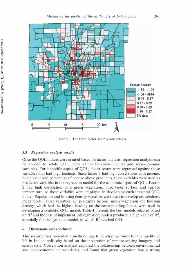
environment quality. Factor 3 shows high positive factor loadings on population

density and housing density, thus is related to crowdedness. The higher the score in

factor 3, the smaller the space for people to live.

The factor scores can be used as indices to represent the quality of life in different

dimensions. The distribution of each factor was mapped in figures 3, 4 and 5

Table 3. Rotated factor loading matrix.

Factor 1 Factor 2 Factor 3

Population density 20.178 20.085 0.953House density 20.116 20.132 0.958Green vegetation 0.159 0.940 20.153Impervious surface 20.328 20.905 20.061Temperature 20.283 20.716 0.472Median household income 0.835 0.295 20.230Median family income 0.885 0.244 20.176Per capita income 0.918 0.168 20.129Percentage of college graduates 0.871 0.152 20.070Median house value 0.853 0.174 20.069

Initial eigenvalues 5.520 1.770 1.430% of variance 40.67 24.69 21.56Cumulative % 40.67 65.36 87.21

Figure 3. The first factor scores: economic index.


Dow

nloa

ded

By: [

Wen

g, Q

.] At

: 21:

10 2

8 M

arch

200

7

respectively. Factor 1, the economic sector of QOL, has a similar distribution

pattern as per capita income because it has the largest loading on per capita income

variable. Similarly, factor 2, the environmental sector, has a distribution pattern

similar to that of green vegetation. Factor 3, which represents crowdedness, has a

similar distribution with housing density. It is noted that there were some non-

residential block groups lacking data because these block groups missed at least one

type’s socioeconomic variable.

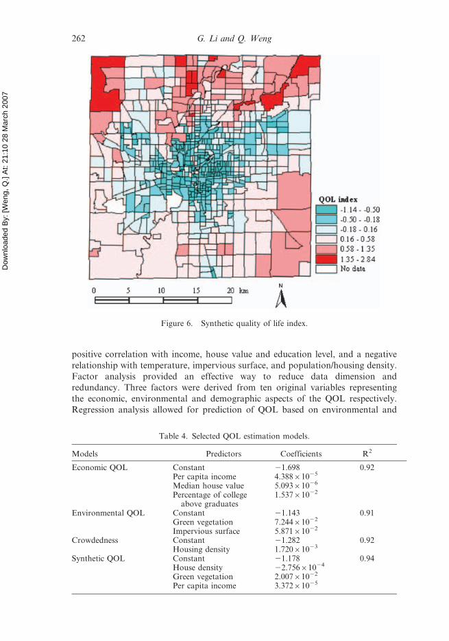
Development of a synthetic QOL index involved the combination of the three

factors that represent different aspects of quality of life. Factor 1 and factor 2 have a

positive contribution to quality of life, while factor 3 has a negative correlation to

QOL. The aggregate score for each block group was then obtained by adding

weighted factor scores of the three factors using the equation below:

QOL~ 40:666�factor1z24:689�factor2{21:859�factor3ð Þ=

Figure 6 shows the distribution of QOL scores. The QOL scores ranged from

21.15 to 2.84. About 5% of block groups had scores greater than 0.9, and most of

them were found in the surrounding areas of the county, especially to the north.

These block groups were characterized by low population density, large green

vegetation coverage, low temperature, less impervious surface and high family

income. Block groups with scores ranging from 21.15 to 20.3 accounted for 30%.

Most of them were found in the city center, which were characterized by less green

vegetation, high population density, and low per capita income.

Figure 4. The second factor scores: environmental index.


100 ð2Þ

Dow

nloa

ded

By: [

Wen

g, Q

.] At

: 21:

10 2

8 M

arch

200

7

5.3 Regression analysis results

Once the QOL indices were created based on factor analysis, regression analysis can

be applied to relate QOL index values to environmental and socioeconomic

variables. For a specific aspect of QOL, factor scores were regressed against those

variables that had high loadings. Since factor 1 had high correlations with income,

home value and percentage of college above graduates, these variables were used as

predictive variables in the regression model for the economic aspect of QOL. Factor

2 had high correlation with green vegetation, impervious surface and surface

temperature, so these variables were employed in developing environmental QOL

model. Population and housing density variables were used to develop crowdedness

index model. Three variables, i.e. per capita income, green vegetation and housing

density, which had the highest loading on the corresponding factor, were used in

developing a synthetic QOL model. Table 4 presents the best models selected based

on R2 and the ease of implement. All regression models produced a high value of R2,

especially for the synthetic model, in which R2 reached 0.94.

6. Discussions and conclusion

This research has presented a methodology to develop measures for the quality of

life in Indianapolis city based on the integration of remote sensing imagery and

census data. Correlation analysis explored the relationship between environmental

and socioeconomic characteristics, and found that green vegetation had a strong

Figure 5. The third factor score: crowdedness.


Dow

nloa

ded

By: [

Wen

g, Q

.] At

: 21:

10 2

8 M

arch

200

7

positive correlation with income, house value and education level, and a negative

relationship with temperature, impervious surface, and population/housing density.

Factor analysis provided an effective way to reduce data dimension and

redundancy. Three factors were derived from ten original variables representing

the economic, environmental and demographic aspects of the QOL respectively.

Regression analysis allowed for prediction of QOL based on environmental and

Figure 6. Synthetic quality of life index.

Table 4. Selected QOL estimation models.

Models Predictors Coefficients R2

Economic QOL Constant 21.698 0.92Per capita income 4.38861025

Median house value 5.09361026

Percentage of collegeabove graduates

1.53761022

Environmental QOL Constant 21.143 0.91Green vegetation 7.24461022

Impervious surface 5.87161022

Crowdedness Constant 21.282 0.92Housing density 1.72061023

Synthetic QOL Constant 21.178 0.94House density 22.75661024

Green vegetation 2.00761022

Per capita income 3.37261025


Dow

nloa

ded

By: [

Wen

g, Q

.] At

: 21:

10 2

8 M

arch

200

7

socioeconomic variables. An important issue encountered was how to integrate

different indicators into a synthetic index. There is currently not a compelling theory

for combing different indicators into one index (Schyns and Boelhouwer 2004).

Because of the lack of available criteria for weighing the indicators, this study

applied a rather pragmatic solution: factors as composite indicators and the

percentage of variance that a factor explains as associated weights.

This research has also demonstrated that GIS can provide an effective platform

for integrating different data models from different data source such as remote

sensing and census socioeconomic data, and for creating a comprehensive database

to assess the QOL. This would help urban managers and policy makers in

formulating the strategies of urban development plans. However, several issues

raised in the integration of disparate data should be concerned. Remote sensing and

census data are collected for ‘different purpose, at different scale, and with different

underlying assumptions about the nature of the geographic features’ (Huang and

Yasuoka 2000). Remote sensing data are digital records of spectral information

about ground features with raster format, and often exhibit continuous spatial

variation. Census socioeconomic data usually relate to administrative units such as

block, block group, tract, county and state, and tend to be more discrete in nature

with sharp discontinuities between adjacent areas. More often, socioeconomic data

are integrated into vector GIS as the attributes of its spatial units for various

mapping and spatial analysis purposes. Integration between remote sensing and

GIS/socioeconomic data involves the conversion between data models. In this study,

remote sensing data were aggregated to census block groups with raster-to-vector

conversion, which assumes that values were uniform throughout block groups. That

would lead to loss of spatial information existing in remote sensing data. In

addition, census has different scales (levels), integration of remote sensing data with

different scales of census data would produce so-called modifiable area unit

problem. Therefore, finding desirable aggregation units is important in order to

reduce the loss of spatial information from remote sensing. Another method of data

integration is through vector-to-raster by rasterization or surface interpolation to

produce a raster layer for each socioeconomic variable. More research is needed on

disaggregating census data into individual pixels to match remote sensing data for

the purpose of data integration.

QOL is a great research topic and concerns many different aspects of the life of

human beings. There has been a great increase in amount of time, efforts and

resources that have been concentrated on quality of life studies. Over 200

communities in the USA and over 589 in the world have conducted QOL indicator

projects, and many of these projects are in the early stages of identifying indicators,

collecting data, reporting result and making recommendations for the using

information that indicators provide (Barsell and Maser 2004). However, there are

still vast differences of opinions on the indicators and ingredients of QOL. Ideally,

QOL research needs to incorporate every dimension of QOL and combine objective

and subjective measurements together. In order to conduct such huge project, the

coalition between different organization such as non-governmental and local

government is necessary. Owing to difficulties to collect all data related to QOL,

especially for detailed geographic unit like census block group, this study is

conducted only from socio-economic and environmental perspectives and explores

spatial variations of QOL, which may help city planners to understand problems,

and to find solutions to issues the community faces.


Dow

nloa

ded

By: [

Wen

g, Q

.] At

: 21:

10 2

8 M

arch

200

7

ReferencesADAMS, J.B., SABOL, D.E., KAPOS, V., FILHO, R.A., ROBERTS, D.A., SMITH, M.O. and

GILLESPIE, A.R., 1995, Classification of multispectral images based on fractions of

endmembers: Application to land cover change in the Brazilian Amazon. Remote

Sensing of Environment, 52, pp. 137–154.

AGUIAR, A.P.D., SHIMABUKURO, Y.E. and MASCARENHAS, N.D.A., 1999, Use of synthetic

bands derived from mixing models in the multispectral classification of remote sensing

images. International Journal of Remote Sensing, 20, pp. 647–657.

ANDREW, K., 1999, Quality of life in cities. Cities, 16, pp. 221–222.

ANDREWS, M.F. and WHITNEY, B.S., 1976, Social indicators of well-being (New York: Plenum

Press).

ASNER, G.P. and LOBELL, D.B., 2000, A biogeophysical approach for automated SWIR

unmixing of soils and vegetation. Remote Sensing of Environment, 74, pp. 99–112.

BARSELL, K. and MASER, E., 2004, Taking indicators to the next level: Truckee Meadows

tomorrow launches quality of life compacts. In Community Quality of life Indicators,

Social Indicators Research Series, M.J. Sirgy, D.R. Rahtz and D.-J. Lee (Eds) Vol. 22

(Kluwer Academic, Dordrecht/Boston/London), pp. 53–74.

BEDERMAN, S.H. and HARTSHORN, T.A., 1984, Quality of life in Georgia: the 1980 experience.

Southeastern Geographer, 24, pp. 78–98.

BONAIUTO, M., FORNARA, F. and BONNES, M., 2003, Indexes of perceived residential

environment quality and neighborhood attachment in urban environment: a

confirmation study on the city of Rome. Landscape and Urban Planning, 65, pp.

41–52.

BURROUGH, P.A., 1986, Principals of geographical information systems for land resource

assessment (New York: Clarendon Press).

CHENG, J. and MASSER, I., 2003, Urban growth pattern modeling: A case study of Wuhan

city, PR, China. Landscape and Urban Planning, 62, pp. 199–217.

COCHRANE, M.A. and SOUZA, Jr. C.M., 1998, Linear mixture model classification of burned

forests in the eastern Amazon. International Journal of Remote Sensing, 19, pp.

3433–3440.

COMREY, A.L. and LEE, H.B., 1992, A First Course in Factor Analysis, 2nd edition (New

Jersey: Erlbuum, Hillsdale).

DOUCETTE, P., AGOOURIS, P. and STEFANIDIS, A., 2004, Automated road extraction from

high resolution multispectral imagery. Photogrammetric Engineering and Remote

Sensing, 70, pp. 1405–1416.

DONNAY, J.P., BARNSLEY, J.M. and LONGLEY, A.P., 2001, Remote sensing and urban

analysis. In Remote Sensing and Urban Analysis, J.P. Donnay, M.J. Barnsley and P.A.

Longley (Eds) (New York: Taylor and Francis).

EHLERS, M., JADKOWSKI, M.A., HOWARD, R.R. and BROSTUEN, D.E., 1990, Application of

SPOT data for regional growth analysis and local planning. Photogrammetric

Engineering and Remote Sensing, 56, pp. 175–180.

FOO, T.S., 2001, Quality of life in cities. Cities, 18, pp. 1–2.

FORSTER, B., 1985, An examination of some problems and solutions in monitoring urban

areas from satellite platforms. International Journal of Remote Sensing, 6, pp.

139–151.

FREY, H.W., 2001, Melting pot suburbs: A census 2000 study of suburban diversity. Census

2000 Series, June (Washington, DC: The Brookings Institution).

FRIEDMAN, M., 1997, Improving the Quality of Life: A Holistic Scientific Strategy

(Connecticut/London: Westport), pp. 19–57.

GREEN, N.E., 1957, Aerial photographic interpretation and the social structure of the city.

Photogrammetric Engineering, 23, pp. 89–96.

HAACK, B., BRYANT, N. and ADAMS, S., 1987, Assessment of Landsat MSS and TM data for

urban and near-urban land cover digital classification. Remote Sensing of

Environment, 21, pp. 201–213.


Dow

nloa

ded

By: [

Wen

g, Q

.] At

: 21:

10 2

8 M

arch

200

7

HALL, G.B., MALCOLM, N.W. and PIWOWAR, J.M., 2001, Integration of remote sensing and

GIS to detect pockets of urban poverty: the case of Rosario, Argentina. Transactions

in GIS, 5, pp. 235–253.

HARRIS, R.J. and LONGLEY, P.A., 2000, New data and approaches for urban analysis:

modeling residential densities. Transactions in GIS, 4, pp. 217–234.

HARRIS, P.M. and VENTURA, S.J., 1995, The integration of geographic data with remote

sensed imagery to improve classification in an urban area. Photogrammetric


HARVEY, J., 2000, Small area population estimation using satellite imagery. Transactions in

GIS, 4, pp. 611–633.

HARVEY, J.T., 2002, Estimation census district population from satellite imagery: some

approaches and limitations. International Journal of Remote Sensing, 23, pp.

2071–2095.

HARVEY, W., MCGLONE, J.C., MCKEOWN, D.M. and IRVINE, J.M., 2004, User-centric

evaluation of semi-automated road network extraction. Photogrammetric Engineering

and Remote Sensing, 70, pp. 1353–1364.

HUANG, T. and YASUOKA, Y., 2000, Integration and application of socio-economic and

environmental data within GIS for development study in Thailand. Available online

at: http://www.gisdevelopment.net/aars/acrs/2000/ts7/gdi004pf.htm.

KAISER, H., 1960, The application of electronic computers to factor analysis. Educational and

psychology, 52, pp. 621–652.

KAMP, I.V., LEIDELMEIJER, K., MARSMAN, G. and HOLLANDER, A.U., 2003, Urban

environmental quality and human well-being towards a conceptual framework and

demarcation of concepts; a literature study. Landscape and Urban Planning, 65, pp.

5–18.

KIM, T., PARK, S., KIM, M., JEONG, S. and KIM, K., 2004, Tracking road centerlines from

high resolution remote sensing images by least squares correlation matching.

Photogrammetric Engineering and Remote Sensing, 70, pp. 1417–1422.

LACOSTE, C., DESCOMBES, X. and ZERUBIA, J., 2002, A comparative study of point processes

for line network extraction in remote sensing. Research Report 4516 (France: INRIA).

LANGFORD, M., MAGUIRE, D.J. and UNWIN, D.J., 1991, The areal interpolation problem:

Estimating population using remote sensing in a GIS framework. In Handling

Geographical Information: Methodology and Potential Applications, L. Masser and M.

Blakemore (Eds) (New York: Longman Scientific & Technical co-published in the

United States with John Wiley).

LI, G. and WENG, Q., 2005, Using Landsat ETM + imagery to measure population density in

Indianapolis, Indiana, USA. Photogrammetric Engineering and Remote Sensing, 71,

pp. 947–958.

LO, C.P., 1995, Automated population and dwelling unit estimation from high resolution

satellite images: a GIS approach. International Journal of Remote Sensing, 16, pp.

17–34.

LO, C.P. and FABER, B.J., 1997, Integration of Landsat Thematic Mapper and census data for

quality of life assessment. Remote Sensing of Environment, 62, pp. 143–157.

LU, D., MORAN, E. and BATISTELLA, M., 2003, Linear mixture model applied to Amazonian

vegetation classification. Remote Sensing of Environment, 87, pp. 456–469.

LU, D. and WENG, Q., 2004, Spectral mixture analysis of the urban landscapes in Indianapolis

city with Landsat ETM + Imagery. Photogrammetric Engineering and Remote Sensing,

70, pp. 1053–1062.

MARTIN, D., TATE, N.J. and LANGFORD, M., 2000, Refining population surface models:

experiments with Northern Ireland census data. Transactions in GIS, 4, pp. 343–360.

MCGWIRE, K., MINOR, T. and FENSTERMAKER, L., 2000, Hyperspectral mixture modeling for

quantifying sparse vegetation cover in arid environments. Remote Sensing of



Dow

nloa

ded

By: [

Wen

g, Q

.] At

: 21:

10 2

8 M

arch

200

7

MESEV, V., 1998, The use of census data in urban image classification. Photogrammetric


METIVIER, E.D. and MCCOY, R.M., 1971, Mapping urban poverty housing from aerial

photographs, Proceedings of the Seventh International Symposium on Remote Sensing

of Environment, (Ann Arbor: University of Michigan Press), pp. 1563–1569.

MUMBOWER, L.E. and DONOGHUE, J., 1967, Urban poverty study. Photogrammetric

Engineering, 33, pp. 610–618.

MUSTARD, J.F. and SUNSHINE, J.M., 1999, Spectral analysis for earth science: investigations

using remote sensing data. In Remote Sensing for the Earth Sciences: Manual of

Remote Sensing, A.N. Rencz (Ed.) Vol. 3 (New York: John Wiley & Sons Inc.).

NICHOL, J. and WONG, M.S., 2005, Modeling urban environmental quality in a tropical city.

Landscape and Urban Planning, 73, pp. 49–58.

ORDWAY, S., 1953, Resources and the American Dream: Including a Theory of the Limit of

Growth (New York: Ronald Press).

OSBORN, F., 1954, The Limits of the Earth (Boston: Little, Brown and Co.).

PACIONE, M., 2003, Urban environmental quality and human wellbeing—a social

geographical perspective. Landscape and Urban Planning, 65, pp. 19–30.

PATHAN, S.K., SASTRY, S.V.C., DHINWA, P.S., MUKUND, R. and MAJUMDAR, K.L., 1993,

Urban growth trend analysis using GIS techniques: a case study of the Bombay

metropolitan region. International Journal of Remote Sensing, 14, pp. 3169–3179.

PHINN, S., STANFORD, M., SCARTH, P., MURRAY, A.T. and SHYY, P.T., 2002, Monitoring the

composition of urban environments based on the vegetation-impervious surface-soil

(VIS) model by subpixel analysis techniques. International Journal of Remote Sensing,

23, pp. 4131–4153.

QIU, F., WOLLER, K.L. and BRIGGS, R., 2003, Modeling urban population growth from

remotely sensed imagery and TIGER GIS road data. Photogrammetric Engineering

and Remote Sensing, 69, pp. 1031–1042.

RASHED, T., WEEKS, J.R., GADALLA, M.S. and HILL, A.G., 2001, Revealing the anatomy of

cities through spectral mixture analysis of multispectral satellite imagery: a case study

of the Greater Cairo region, Egypt. Geocarto International, 16, pp. 5–15.

ROBERTS, D.A., BATISTA, G.T., PEREIRA, J.L.G., WALLER, E.K. and NELSON, B.W., 1998,

Change identification using multitemporal spectral mixture analysis: applications in

eastern Amazonia. In Remote Sensing Change Detection: Environmental Monitoring

Methods and Applications, R.S. Lunetta and C.D. Elvidge (Eds) (Chelsea, Michigan:

Ann Arbor Press), pp. 137–161.

SCHYNS, P. and BOELHOUWER, J., 2004, The state of city Amsterdam monitor: measuring

Quality of life in Amsterdam. In Community Quality of life Indicators, Social

Indicators Research Series, M.J. Sirgy, D.R. Rahtz and D-J. Lee (Eds) Vol. 22 Kluwer

Academic: Dordrecht/Boston/London), pp. 133–152.

SMALL, C., 2001, Estimation of urban vegetation abundance by spectral mixture analysis.

International Journal of Remote Sensing, 22, pp. 1305–1334.

SMITH, D.M., 1973, The Geography of Social Well-being in the United State (New York:

McGraw-Hill).

SMITH, M.O., USTIN, S.L., ADAMS, J.B. and GILLESPIE, A.R., 1990, Vegetation in deserts: I. A

regional measure of abundance from multispectral images. Remote Sensing of


SONG, M. and CIVCO, D., 2004, Road extraction using SVM and image segmentation.

Photogrammetric Engineering and Remote Sensing, 70, pp. 1365–1372.

SUTTON, P., 1997, Modeling population density with nighttime satellite imagery and GIS.

Computers, Environment and Urban Systems, 21, pp. 227–244.

TABACHNICK, B. and FIDELL, L., 1996, Using Multivariate Statistics, 3rd edition (New York:

Harper Collins College).

THOMSON, C.N., 2000, Remote sensing/GIS integration to identify potential low-income

housing sites. Cities, 17, pp. 97–109.


Dow

nloa

ded

By: [

Wen

g, Q

.] At

: 21:

10 2

8 M

arch

200

7

TREITZ, P.M., HOWARD, P.J. and GONG, P., 1992, Application of satellite and GIS

technologies for land-cover and land-use mapping at the rural-urban fringe: a case

study. Photogrammetric Engineering and Remote Sensing, 58, pp. 439–448.

WEBER, C. and HIRSCH, J., 1992, Some urban measurements from SPOT data: urban life

quality indices. International Journal of Remote Sensing, 13, pp. 3251–3261.

WELCH, R., 1982, Spatial resolution requirements for urban studies. International Journal of

Remote Sensing, 3, pp. 139–146.

WENG, Q., 2001, A remote sensing-GIS evaluation of urban expansion and its impact on

surface temperature in the Zhujiang Delta, China. International Journal of Remote

Sensing, 22, pp. 1999–2014.

WENG, Q., 2002, Land use change analysis in the Zhujiang Delta of China using satellite

remote sensing, GIS, and stochastic modeling. The Journal of Environmental

Management, 64, pp. 273–284.

WENG, Q., LU, D. and SCHUBRING, J., 2004, Estimation of land surface temperature–

vegetation abundance relationship for urban heat island studies. Remote Sensing of


WILKINSON, G.G., 1996, A review of current issues in the integration of GIS and remote

sensing data. International Journal of Geographic Information Systems, 10, pp. 85–101.

WU, C. and MURRAY, A.T., 2003, Estimating impervious surface distribution by spectral

mixture analysis. Remote Sensing of Environment, 84, pp. 493–505.

YEH, A.G.O. and LI, X., 1997, An integrated remote sensing and GIS approach in the

monitoring and evaluation of rapid urban growth for sustainable development in the

Pearl River Delta, China. International Planning Studies, 2, pp. 193–210.

YUAN, Y., SMITH, R.M. and LIMP, W.F., 1997, Remodeling census population with spatial

information from Landsat imagery. Computers, Environment and Urban Systems, 21,

pp. 245–258.


Documents

Measuring the quality of life in city of Indianapolis by