Embed Size (px)
Citation preview
Wesleyan University The Honors College
Measuring the Local ISM Along theSight Lines of the Two Voyager
Spacecraft with HST/STIS
by
Julia R. ZacharyClass of 2017
A thesis submitted to thefaculty of Wesleyan University
in partial fulfillment of the requirements for theDegree of Bachelor of Arts
with Departmental Honors in Astronomy
Middletown, Connecticut April, 2017

Look again at that dot. That’s here. That’s home. That’s us. On
it everyone you love, everyone you know, everyone you ever heard of,
every human being who ever was, lived out their lives. The aggregate
of our joy and suffering, thousands of confident religions, ideologies,
and economic doctrines, every hunter and forager, every hero and cow-
ard, every creator and destroyer of civilization, every king and peasant,
every young couple in love, every mother and father, hopeful child, in-
ventor and explorer, every teacher of morals, every corrupt politician,
every “superstar,” every “supreme leader,” every saint and sinner in
the history of our species lived there−on a mote of dust suspended in
a sunbeam.
–Carl Sagan
Pale Blue Dot: A Vision of Human Future in Space

Acknowledgements
First and foremost, I want to thank my adviser, Seth Redfield, who tirelessly
and unfailingly answered all my many questions. Without your guidance and
knowledge, I would’ve never done this research and written this thesis.
Thank you to professors whose advice or input I sought over the course of
this year: Meredith Hughes, Ed Moran, Christina Othon, and Roy Kilgard. I’m
always grateful for when you take time out of your day to talk with me.
My fellow thesisers: JD, GD, SW. It’s been a loooooong road, from starting
off together in 155 to now finishing our senior theses. Glad I did it with you guys.
To CE, CW, AH, AR, AW, NS, and MS: You are all some of my very best
friends at Wes. It’s been quite the adventure!
To JKS, KMM: I am so glad I’ve been able to spend my whole life with you
as my friends.
To the physics crew: It’s been a wild ride. Thank you for working on/struggling
through homework with me for four years.
Of course, to my family: Thank you for letting me talk your ears off about
astronomy for the last four years. Thank you for your constant love and support.
I love you.

Contents
1 Introduction 1
1.1 Voyager . . . . . . . . . . . . . . . . . . . . . . . . . . . . . . . . 1
1.2 The Structure of the Heliosphere . . . . . . . . . . . . . . . . . . 5
1.2.1 Interplanetary Magnetic Fields . . . . . . . . . . . . . . . 6
1.2.2 Heliospheric Termination Shock . . . . . . . . . . . . . . . 7
1.2.3 The Heliosheath, Heliopause, and Beyond . . . . . . . . . 8
1.3 The Nature of the Interstellar Medium . . . . . . . . . . . . . . . 11
1.3.1 Interstellar Magnetic Fields . . . . . . . . . . . . . . . . . 13
1.3.2 Gas Clouds . . . . . . . . . . . . . . . . . . . . . . . . . . 14
1.3.3 Dust Grains . . . . . . . . . . . . . . . . . . . . . . . . . . 15
1.3.4 Kinematic Structure . . . . . . . . . . . . . . . . . . . . . 16
1.4 Hubble Space Telescope . . . . . . . . . . . . . . . . . . . . . . . . 18
1.5 Connections to Voyager . . . . . . . . . . . . . . . . . . . . . . . 20
2 Observations and Data Reduction 21
2.1 Space Telescope Imaging Spectrograph . . . . . . . . . . . . . . . 21
2.2 Observations . . . . . . . . . . . . . . . . . . . . . . . . . . . . . . 22
2.3 Data Reduction . . . . . . . . . . . . . . . . . . . . . . . . . . . . 25
2.4 Target Stars . . . . . . . . . . . . . . . . . . . . . . . . . . . . . . 26
3 Fitting and Results 28
3.1 Interstellar Ions . . . . . . . . . . . . . . . . . . . . . . . . . . . . 28
3.2 The Fitting Procedure . . . . . . . . . . . . . . . . . . . . . . . . 30
3.2.1 Continuum . . . . . . . . . . . . . . . . . . . . . . . . . . 30
3.2.2 ISM Absorption . . . . . . . . . . . . . . . . . . . . . . . . 32
3.2.3 Error Analysis . . . . . . . . . . . . . . . . . . . . . . . . . 34
3.3 Fits . . . . . . . . . . . . . . . . . . . . . . . . . . . . . . . . . . . 35
3.4 Fit Parameters . . . . . . . . . . . . . . . . . . . . . . . . . . . . 41
3.4.1 Velocity Offsets . . . . . . . . . . . . . . . . . . . . . . . . 43
3.4.2 Geocoronal Features . . . . . . . . . . . . . . . . . . . . . 44
3.5 The Lyman α Profile . . . . . . . . . . . . . . . . . . . . . . . . . 49
4 Analysis of Physical Parameters 53
4.1 Comparing with the Kinematic Model . . . . . . . . . . . . . . . 53
4.1.1 The Voyager 1 Sight Line . . . . . . . . . . . . . . . . . . 55
4.1.2 The Voyager 2 Sight Line . . . . . . . . . . . . . . . . . . 56
4.2 Temperature and Turbulence . . . . . . . . . . . . . . . . . . . . . 58
4.3 Abundance and Depletion . . . . . . . . . . . . . . . . . . . . . . 64
4.4 Electron Density . . . . . . . . . . . . . . . . . . . . . . . . . . . 67
4.4.1 Comparisons to Voyager . . . . . . . . . . . . . . . . . . . 70
5 Conclusions and Future Work 73
5.1 Future Work . . . . . . . . . . . . . . . . . . . . . . . . . . . . . . 74
5.2 The “Interstellar Road Map” . . . . . . . . . . . . . . . . . . . . 78
Bibliography 82
Chapter 1
Introduction
The general purpose of this thesis is to explore the structure and composition
of the local interstellar medium using Hubble Space Telescope spectra coupled with
in situ Voyager observations. In order to discuss the importance of the analysis
that will be subsequently presented, I will first introduce the various components
of my research, including the spacecraft and telescope, as well as the structural
components of the heliosphere and interstellar medium. The following chapter
provides an overview and background to the entire project to allow for a complete
introduction to the topic of the interstellar medium. Many interstellar medium
observations have been taken with the Hubble Space Telescope, but never before
have those observations been combined with data from a spacecraft actually in
the interstellar medium. The Voyager spacecraft represent a new frontier in inter-
stellar medium research, presenting the first ever in situ interstellar observations.
1.1 Voyager
On September 5, 1977, the Voyager 1 spacecraft was launched from the NASA
Kennedy Space Center at Cape Canaveral, Florida. Voyager 1 and its counterpart,
Voyager 2, which was launched a month earlier, were to study the interplanetary
space between Earth and Saturn, explore the Saturnian and Jovian planetary
systems, and, if possible, extend the mission to Uranus and Neptune (Kohlhase &
1. Introduction 2
Penzo 1977). The mission was conceived out of the idea for a “grand tour” of the
outer Solar System. This grand tour was initiated due to a fortuitous planetary
alignment, and Voyager 2 was able to travel to all four giant planets (Sagan
1994; Rudd et al. 1997). Voyager 1 ’s slightly-less grand tour included traveling
to Jupiter, Saturn, and Titan, one of the largest of the Saturnian moons. By the
end of 1989, it was clear that both spacecraft were heading on separate paths
out of the ecliptic plane. Voyager 1 was headed north after being boosted by
Saturn, and Voyager 2 was headed south after its encounter with Neptune at an
angle nearly perpendicular to Voyager 1 (Rudd et al. 1997). An extension of the
original Voyager mission, the Voyager Interstellar Mission (VIM) intended to not
only continue investigating the interplanetary medium, but also to characterize
the structure of the heliosphere and begin studying the interstellar medium (Rudd
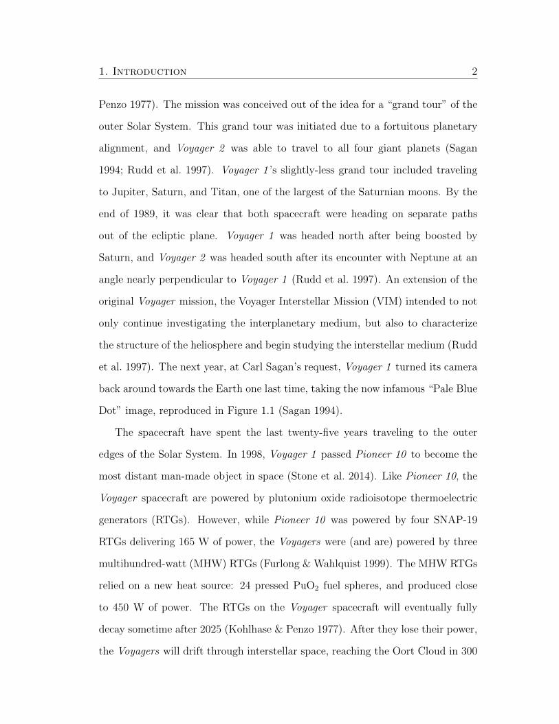
et al. 1997). The next year, at Carl Sagan’s request, Voyager 1 turned its camera
back around towards the Earth one last time, taking the now infamous “Pale Blue
Dot” image, reproduced in Figure 1.1 (Sagan 1994).
The spacecraft have spent the last twenty-five years traveling to the outer
edges of the Solar System. In 1998, Voyager 1 passed Pioneer 10 to become the
most distant man-made object in space (Stone et al. 2014). Like Pioneer 10, the
Voyager spacecraft are powered by plutonium oxide radioisotope thermoelectric
generators (RTGs). However, while Pioneer 10 was powered by four SNAP-19
RTGs delivering 165 W of power, the Voyagers were (and are) powered by three
multihundred-watt (MHW) RTGs (Furlong & Wahlquist 1999). The MHW RTGs
relied on a new heat source: 24 pressed PuO2 fuel spheres, and produced close
to 450 W of power. The RTGs on the Voyager spacecraft will eventually fully
decay sometime after 2025 (Kohlhase & Penzo 1977). After they lose their power,
the Voyagers will drift through interstellar space, reaching the Oort Cloud in 300

1. Introduction 3
Figure 1.1: Taken by Voyager 1 in 1990, this image shows Earth as it looked from 4billion miles away. At this distance, Earth is just a tiny point of light just over a tenthof a pixel in size (seen in the center-right of this image).
1. Introduction 4
years, with Voyager 2 passing by Sirius in ∼300,000 years (Rudd et al. 1997).
Out of the eleven scientific instruments originally operational on the Voyagers,
only five are currently still operational (Rudd et al. 1997). These instruments are
now crucial to providing insight into the composition, structure, and presence of
the various components of the heliosphere and interstellar space. One of the most
important instruments is the Cosmic Ray Subsystem (CRS), which uses three in-
dependent solid state detector telescopes to take direct measurements of galactic
cosmic ray intensities (Stone et al. 1977). These telescopes allows for the detection
and measurement of low-energy galactic cosmic rays, which provide information
about particle acceleration and interstellar propagation (Stone et al. 1977). The
Low Energy Charged Particle (LECP) experiments involve using two detectors
on each spacecraft to measure the differential in energy fluxes and angular dis-
tributions of both ions and electrons (Krimigis et al. 1977). The magnetometers
on-board the Voyagers provide measurements of the magnetic fields of both plane-
tary and interplanetary media, which are crucial to understanding the structure of
the heliosphere. Other still functioning instruments include the ultraviolet spec-
trometer and the Plasma Wave System (PLS). Since basic planetary dynamical
processes are often associated with wave-particle interactions, the PLS provides an
understanding of these processes by measuring electric field components between
10 Hz−56 kHz (Scarf & Gurnett 1977).
On August 25, 2012, the Voyager Interstellar Mission team received direct
confirmation that Voyager 1 had entered interstellar space (Gurnett et al. 2013).
It is expected that Voyager 2 will exit the heliosphere within the next couple
of years (Stone et al. 2014). For the first time, humans have sent a spacecraft
outside the confines of the Solar System, which for thousands of years seemed to
be the boundary of the known universe. As of April 19, 2017, Voyager 1 is in

1. Introduction 5
interstellar space at at a distance of 137.73 AU from Earth, and Voyager 2 is in the
heliosheath at 114.0 AU from Earth.1 The two spacecraft are the fastest-moving
human-made objects, travelling at 3.6 AU/year and 3.3 AU/year, respectively
(Stone et al. 2005).
1.2 The Structure of the Heliosphere
The volume of interplanetary space through which the Voyagers have spent
much of their mission traveling is known as the heliosphere. It can be thought
of as a giant bubble enclosing the Sun and planets, protecting the Solar System
from high energy cosmic rays. This bubble is formed by the solar wind coming
into contact with the gas and magnetic fields of the interstellar medium (Mewaldt
& Liewer 2000). The solar wind is actually plasma emanating from the Sun at
speeds of 400−700 km s−1 (Stone et al. 2014). The heliosphere not only shields
the Solar System from cosmic rays, but also guards against interstellar plasma,
fields, and dust (Mewaldt & Liewer 2000). Because the heliosphere is moving with
respect to the interstellar medium, its shape is affected by pressure dynamics. In
the upwind direction, there is a compressed “nose,” and conversely, a downwind
“tail” (McComas et al. 2012).
As the solar wind moves out from the Sun, it eventually comes into contact
with much cooler interstellar plasma, creating a boundary known as the heliopause
(Gurnett et al. 2013). The heliopause is considered to be the edge of the helio-
sphere (Stone et al. 2014). It takes up to a year for the solar wind to reach the
outer edges of the heliosphere, during which the wind evolves significantly over
such large distances. Coronal mass ejections overtake the slower solar wind, pro-
1http://voyager.jpl.nasa.gov/where/index.html
1. Introduction 6
ducing compressed regions known as merged interaction regions (MIRs). MIRs
are associated with enhanced magnetic field magnitudes and fluctuations, and can
also be related to shocks in the solar wind, where speeds can increase or decrease
rapidly (Richardson et al. 2008).
1.2.1 Interplanetary Magnetic Fields
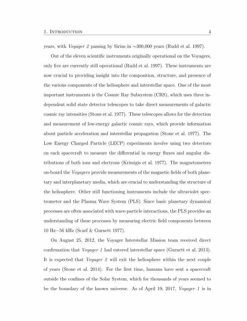
As seen in Figure 1.2, the interplanetary and solar magnetic fields are carried
by the solar wind, forming a spiral structure. This structure has origins in the
coronal magnetic field, which is driven by the motion of plasma in the photosphere
of the Sun (Owens & Forsyth 2013). The magnetic field lines of the heliosphere are
fixed in the photosphere, rotating with the Sun. Because the magnetic field lines
remain “frozen,” the rotation causes twisting, forcing the field into a spiral (Parker
1958; Owens & Forsyth 2013). Once the solar wind achieves supersonic speeds, it
drags the plasma out into the heliosphere, forming the heliospheric magnetic field.
In addition to the supersonic solar wind, there is a belt of slower-moving material
(300−400 km s−1) that originates from the region corresponding to the magnetic
equator (Owens & Forsyth 2013). This slow solar wind belt is only about 20 in
latitudinal width, but contributes enough to form the heliospheric current sheet,
which is formed by the magnetic field boundary separating opposing magnetic field
lines (Owens & Forsyth 2013). Interplanetary magnetic fields are highly variable
on scales of 1 day to several solar rotations as the solar wind flows outward. That
the Voyager spacecraft observed these fluctuations is no surprise, but some of
the physical properties it measured were surprising. The magnetic field direction
variability creates “sectors” of differing polarity which are based on extensions
of magnetic fields from the polar regions of the Sun to the observing spacecraft.

1. Introduction 7
Figure 1.2: The complex structure of the heliosphere (from Stone et al. 2014).
Voyager 1 observed these sectors throughout its time in the heliospheric current
sheet. Surprisingly, it remained in a positive sector for at least 125 days. Stone
et al. (2005) postured that this sector was caused by reduced speeds behind an
inward moving shock.
1.2.2 Heliospheric Termination Shock
The heliospheric termination shock (HTS) is the boundary where the solar
wind decelerates from a cool supersonic flow to hot subsonic speeds (Burlaga et al.
2005; Stone et al. 2014). The solar wind pick-up ions are slowed, compressed, and
therefore are heated. At the HTS, the solar wind decreases from 400 km s−1 to
∼130 km s−1 in response to inward pressure from the local interstellar medium
(Webber & McDonald 2013; Jokipii 2013). In 2004, Voyager 1 crossed the HTS
at a distance of 94 AU, while Voyager 2 crossed at 84 AU in 2007 (Krimigis

1. Introduction 8
et al. 2009). This inconsistency in the position of the HTS is due to asymmetry
in the heliosphere, which varies with both time and location, as shown in Figure
1.3. Voyager 2 measured the temperature and energy distribution of heliospheric
plasma in the HTS, determining that the expansion of solar wind plasma heats
up the HTS (Richardson et al. 2008). Both in situ and remote observations of the
heliosphere and HTS have shown that the HTS is not perfectly spherical. The
asymmetry is caused by a tilted interstellar magnetic field, which “blunts” the
HTS at an angle relative to the orientation of the magnetic field (Jokipii 2013;
Stone et al. 2014).
1.2.3 The Heliosheath, Heliopause, and Beyond
Beyond the termination shock lies the heliosheath, where the solar wind be-
comes subsonic. The heliosheath is both encompassed within the heliosphere
and extended outward beyond the heliopause. The section located inside the he-
liopause is the inner heliosheath, and likewise, the section outside is the outer
heliosheath (Schwadron et al. 2015). Voyager 1 measured a large increase in in-
terstellar plasma density after crossing the heliopause in 2012 (Voyager 2 has
not yet crossed this boundary, but is predicted to within the next five years).2
The expected interstellar plasma density in the outer heliosheath is 0.1 cm−3, and
Voyager 1 measured values of approximately 0.08 cm−3, which is consistent with
the expected value (Schwadron et al. 2015). Since the solar wind remains sub-
sonic within the heliosheath, neutral interstellar ions can penetrate the heliosphere
(Frisch et al. 2009).
The asymmetry of the HTS and heliosphere is also noted in Figure 1.3 as ex-
isting in the heliosheath. It explains a correlation between anomalous cosmic rays
2http://voyager.jpl.nasa.gov/mission/interstellar.html

1. Introduction 9
Figure 1.3: The contours of the interstellar magnetic field, with strength B(nT),are shown as black lines, while the white lines denote the trajectories of the Voyagerspacecraft. The heliospheric current sheet within the heliosheath is deflected to thenorth (Opher et al. 2006).
(ACRs) and galactic cosmic rays (GCRs) observed (Frisch et al. 2009). ACRs are
formed by the acceleration of pick-up ions, which are ionized interstellar neutral
particles, while GCRs are charged particles, typically protons (Frisch et al. 2009;
Blasi 2013).
At ∼200 AU, there is a region known as the hydrogen wall (H-wall), which
has a higher density of hydrogen atoms. As interstellar plasma flows through
the solar system, it is slowed and heated by exchanges with solar wind protons
(Linsky & Wood 1996). The H-wall results from coupling between the neutral
components of the LISM and the magnetic fields and charged particles within
the heliosphere. The signature of the H-wall is seen towards local stars in their
Lyman-α absorption features (Linsky & Wood 1996).
In Figure 1.3, the interstellar magnetic field is parallel to the hydrogen deflec-
tion plane (HDP), which is defined by hydrogen and helium flow vectors. These

1. Introduction 10
flow vectors differ from each other by only 4, but their directions are similar
enough to constrain the HDP to a plane inclined by 60 to the galactic plane
(Opher et al. 2006). The HDP is also relatively close (within ∼ 2) to the plane
containing the Sun and undisturbed interstellar plasma flows (Grygorczuk et al.
2015).
Past the H-wall would typically be a bow shock, which is where the interstel-
lar medium meets the solar wind, the density and pressure change rapidly, and
the ISM flow slows to subsonic speeds (Sparavigna & Marazzato 2010). McComas
et al. (2012) determined from measurements made by NASA’s Interstellar Bound-
ary Explorer (hereafter, IBEX ) that there is a bow “wave” of enhanced plasma
density. IBEX measured an ISM velocity lower than the previous Ulysses results
indicated (Witte 2004). Because this velocity is lower than the magnetosonic
speed required to produce a shock, McComas et al. (2012) concluded that there is
in fact no bow shock. This conclusion was supplemented by three different mod-
els created by Zank et al. (2013), who used magnetohydrodynamic plasma-kinetic
hydrogen models with current LISM parameters. Their second model, which was
constructed in three dimensions with an interstellar magnetic field strength of 3
µG, yielded a ∼ 200 AU thick shock-free structure.
Additional observations with IBEX revealed a new population of warm in-
terstellar helium within the heliosphere. Kubiak et al. (2014) used detections of
neutral interstellar helium to propose a new velocity-driven structure they call the
“Warm Breeze.” The authors determined that the Warm Breeze is composed of
a secondary population of neutral interstellar helium atoms, but were unable to
definitively conclude on its origins. The most likely hypothesis is that the Warm
Breeze is created due to charge exchange and scattering events between neutral
and singly-ionized helium in the heliosheath (Kubiak et al. 2014). Alternatively,

1. Introduction 11
the Warm Breeze could be simply a gust of neutral helium blown through the local
interstellar cloud in a set of waves, which may be supported by its ∼19 angle to
the inflow of interstellar gas. This difference in inflow directions between hydrogen
and helium was also observed as early as 1977 by Adams & Frisch (Frisch et al.
2009).
1.3 The Nature of the Interstellar Medium
As the Sun travels around the galactic center in its 220 million-year orbit, it
passes through multiple clouds of gas, dust, and plasma. These clouds are the
interstellar medium, or colloquially: the substance between stars. The interstellar
medium contains the repository of building blocks necessary for star formation,
and is replenished by stars at the end of their lifetimes as they deposit material
either in the form of a supernova or a planetary nebula (McCray & Snow 1979).
It therefore serves as a site for future star formation.
The local interstellar medium (LISM) forms the outer boundary for the helio-
sphere, and its behavior dictates the behavior of the Sun and heliosphere (Stone
et al. 2014). The Solar System resides within the Local Bubble, which was formed
by material blowing out of major star-formation regions in Scorpius and Centau-
rus (Mewaldt & Liewer 2000; Malamut et al. 2014). The Local Bubble is a region
of low-density material extending for 50−200 pc within the local galactic neigh-
borhood (Frisch et al. 2011). The Local Bubble includes the circum-heliospheric
interstellar medium (CHISM), which sits at the edge of the Local Interstellar
Cloud (LIC). The CHISM is the progenitor of interstellar gas and dust that flows
through the heliosphere, and is relatively homogenous (Frisch et al. 2009). The
LIC is one of a suite of warm, partially ionized clouds that make up the LISM.

1. Introduction 12
Figure 1.4: Artist’s rendering of the Solar System and local interstellar medium on alogarithmic scale (Stone et al. 2014).
At a certain point, “pristine” ISM interacts with “contaminants,” which con-
tain atoms influenced by the heliosphere. McComas et al. (2015) determined that
the location of the “pristine” ISM depends on the extent of the Sun’s gravitational
influence and the position of the heliospere relative to the interstellar gas upstream
of it in the LISM. The Sun’s Hill Sphere, the region where its gravitational influ-
ence is strongest, extends out to nearly 5000 AU, not quite reaching the estimated
inner edge of the Oort Cloud at 10,000 AU (Oort 1950; Morbidelli 2005; McComas
et al. 2015). At this distance, the gravitational influence from the Galactic disk
begins to take over, and particle interactions in the ISM are unaffected by the
heliosphere. McComas et al. (2015) found that even at a distance of 1000 AU the
ISM can be considered essentially pristine. At this point, gravitational bending
(calculated from analytic solutions) is less than 0.1 and magnetohydrodynamic
simulations show that there is no perturbation by the heliosphere on the LIC
(Zank et al. 2013; McComas et al. 2015).
1. Introduction 13
1.3.1 Interstellar Magnetic Fields
Mentioned briefly in conjunction with the shape of the heliosphere (see Sec-
tions 1.2.1 and 1.2.3), determining direction and magnitude of interstellar mag-
netic fields is key to understanding the interactions between the LISM and the
heliosphere. The strength of interstellar magnetic fields (ISMF) affects the shape
of the helisophere and dictates the filtration of particles streaming into the Solar
System (Opher et al. 2009). Until Voyager 1 crossed the heliopause in 2012, no
in situ measurements were available to directly measure the orientation of the
ISMF. Early methods involved measuring polarization of light from nearby stars
and measuring backscattered solar Lyman α radiation (Opher et al. 2009). Opher
et al. (2006) suggested that a ∼2 µG ISMF in the HDP could account for observa-
tions of energetic shock particles by the Voygager spacecraft, with a field direction
between 38−60. However, the model used by Opher et al. (2006) neglected to
include neutral hydrogen atoms, which led to underestimations of the strength
of the ISMF in addition to large uncertainties in the field direction (Opher et al.
2009). Opher et al. (2009) followed up on the work by Opher et al. (2006) with
new model constraints using Voyager 2 observations of heliosheath flows. The
orientation of the ISMF is determined by both the angle between the ISMF and
the interstellar wind and the angle between the solar equator and the plane formed
by the ISMF and interstellar wind (Opher et al. 2009). In order to account for
the Voyager termination shock crossing distances, Opher et al. (2009) determined
that the ISMF strength had to be between 3.7 and 5.5 µG. Opher et al. (2009) also
noted some discrepancies between their work and previous works with respect to
ISMF orientation angle, and accounted for those differences as the result of ISM
turbulence. ISM turbulence could cause the local magnetic field direction to differ
1. Introduction 14
from that of the large-scale ISMF.
Burlaga & Ness (2016) used Voyager 1 observations to constrain the local
ISMF strength to 0.48 nT (or 4.8 µG), consistent with the range predicted by
models from Opher et al. (2009). Additional modeling by Zirnstein et al. (2016)
with IBEX data produced precise values for the magnitude and direction of pris-
tine ISMF far (>1000 AU) from the Sun. Both sets of authors concluded that in
situ measurements implied a draped strong ISMF around the helisophere.
1.3.2 Gas Clouds
Much of the interstellar medium consists of low density, partially ionized gas
coupled with dust. The ionization state of the gas depends on the local intensity of
ultraviolet radiation needed to photodissociate or photoionize molecules (Draine
2009). Extreme-ultraviolet light from hot stars or white dwarfs provides sources of
photoionization, causing an anisotropic gradient within the Local Bubble (Frisch
et al. 2011). Inhomogeneous LISM clouds were only identified fifty years ago, and
the first spectrum of interstellar gas outside the heliosphere was taken in 1977
with Copernicus (Adams & Frisch 1977; Frisch et al. 2009).
The majority of the LISM clouds consist of warm to hot neutral or ionized gas,
though there are areas of cool gas. Photoionization provides a way to maintain
the warm gas temperatures. Mobius et al. (2004) summarized previous interstellar
helium parameters, including observations of the HeI 5870 A line that provided
measurements for gas temperature. A helium temperature of 6300±340 K was
derived from the measurements taken over the full duration of the Ulysses mission
(Mobius et al. 2004), while temperatures between 5000 and 8000 K have been
measured via long line-of-sight observations for 15 LISM clouds (Redfield & Linsky

1. Introduction 15
2004b). These temperatures were found from measuring the absorption line widths
of elements or ions with varying atomic weights in order to separate the thermal
components from non-thermal ones (Linsky & Redfield 2014).
1.3.3 Dust Grains
In the 1990s, as it flew past Jupiter, Ulysses confirmed the presence of in-
terstellar dust grains within the Solar System (Frisch et al. 2009). The dust, as
expected, traveled with a speed and direction very similar to that of neutral in-
terstellar hydrogen and helium gas. Dust particles have also been found by the
in situ detectors on both Galileo and Cassini (Frisch et al. 2009). The properties
of LISM dust have been inferred and measured by a wide range of techniques,
including extinction and polarization of starlight, scattering, and thermal emis-
sion (Draine 2009). Since the interstellar clouds in the LISM were expected to
be “diffuse clouds” largely consisting of neutral hydrogen and with low extinction
coefficients, it was expected that the Local Bubble would be the same (Draine
2009). Spectroscopic features observed in the infrared showed silicate absorption,
consistent with the assumption that most interstellar dust is composed of silicates
or carbonates. Ulysses discovered that interstellar dust concentrations vary with
solar cycle − that the dust concentration decreased during solar minimum due to
solar wind filtering (Frisch et al. 2009). Ulysses also measured interstellar dust
grain sizes, determining that grain size increased closer to the Sun. These obser-
vations, coupled with those from Galileo and Cassini, concluded that there is a
dearth of small dust grains between 0.7 and 3 AU, implying that the interstellar
dust stream is filtered by solar radiation pressure (Frisch et al. 2009).
Depletion occurs when heavy elements have gas phase abundances that are

1. Introduction 16
less than the expected cosmic abundances, often because of varying levels of in-
corporation into interstellar dust grains. In mathematical terms, depletion can be
defined as either linear or logarithmic, reflecting the linear and logarithmic gas
phase abundances referenced to cosmic or solar abundances (Savage & Sembach
1996). However, one caveat is that depletions do not always take into account
partial ionization of hydrogen (Redfield & Linsky 2008). In the LISM, elemental
depletion gives rise to the need for ionization corrections. The number of atoms
that must be depleted onto dust grains can also be calculated based on pickup ion
isotope ratios (Frisch et al. 2011). Additionally, depletion onto dust grains in the
ISM clouds depends on the condensation temperature of the element in question.
Therefore, elements with the highest condensation temperatures are the most de-
pleted in the ISM, and the gas phase abundances of volatile elements are higher
in warm clouds (Frisch et al. 2011; Savage & Sembach 1996). Small depletions
are well-correlated with high turbulent velocities, suggesting that the destruction
of dust grains may have returned specific ions to their gas phase. It is entirely
possible that dust destruction was caused by shocks produced by supernovae or by
turbulent motions driven by interaction between clouds or even by direct collisions
(Redfield & Linsky 2008).
1.3.4 Kinematic Structure
The kinematic structure of the LISM is fairly complicated, with multiple ab-
sorbers along many sight lines. Early analysis of titanium absorption line spectra
for stars within 100 pc by Crutcher (1982) found that warm gas within the LISM
moves with a coherent heliospheric velocity. Crutcher (1982) determined that the
direction of the gas was consistent with that of an expanding shell of gas acceler-

1. Introduction 17
Figure 1.5: The dynamical cloud morphologies determined by Redfield & Linsky(2008) are overlaid in galactic coordinates and color-coded, with the upwind heliocentricvelocity vector direction indicated by the circled cross and the downwind vector directiongiven by the circled dot. The black outlines indicate sharp edges of the clouds. Theblack stars represent sources of radio scintillation as studied by (Linsky et al. 2008).
ated by both hot stars and supernovae from the Scorpius-Centaurus Association
− the nearest OB association to the Sun (Redfield & Linsky 2015).
Frisch et al. (2002) and Redfield & Linsky (2004a) developed the basis for
the current best kinematic model of the LISM, which was created by Redfield
& Linsky (2008). Redfield & Linsky (2008) based their kinematic model off of
a large data set containing 270 individual velocity components along 157 differ-
ent lines of sight through the LISM. They also used high-resolution Hubble Space
Telescope spectra from the Goddard High Resolution Spectrograph and the Space
Telescope Imaging Spectrograph for 55 velocity components to measure absorp-
tion line width from ions of different atomic weight in order to determine the
temperature and turbulent velocity (Redfield & Linsky 2004b). The model by
Redfield & Linsky (2008) includes 15 distinct clouds. These component clouds
1. Introduction 18
are individual co-moving structures of partially ionized gas identified by common
velocities across large patches of the sky (Redfield & Linsky 2015). In order to de-
termine the morphology of these clouds, Redfield & Linsky (2008) assumed that
the interstellar gas flow inside each cloud is coherent and that the clouds have
sharp edges. The names of these clouds are either historical or based off of their
locations in the sky relative to named constellations (Redfield & Linsky 2008).
1.4 Hubble Space Telescope
The Hubble Space Telescope (HST ) was launched from Cape Canaveral, FL
on April 24, 1990 aboard the Space Shuttle Discovery. The culmination of ten
years and $1.6 billion, HST was designed to be the newest and most advanced
space telescope of its generation and the next (Goodwin & Cioffi 1994). While
launch was originally scheduled for early 1986, the Challenger disaster forced
NASA to delay HST ’s launch and deployment for another four years (Shayler
& Harland 2016). A day after its launch, on April 25, 1990, HST was de-
ployed into a low-Earth orbit at an altitude of approximately 570 km (Xapsos
et al. 2014). The initial main objective of the space telescope initiative pro-
posed by NASA (as early as the early 1970s) was to launch a 2.4 m telescope
“with excellent optical quality into orbit to obtain unmatched spatial resolu-
tion and ultraviolet sensitivity” (Robberto et al. 2000). HST was the first of
NASA’s “Great Observatories” to be launched, and it was swiftly followed by
the Compton Gamma Ray Observatory in 1991, Chandra X-Ray Observatory
in 1999, and the Spitzer Space Telescope in 2003 (Shayler & Harland 2016).
3http://hubblesite.org/image/3831/spacecraft

1. Introduction 19
Figure 1.6: HST as seen from the Space Shuttle Discovery during its second servicingmission in February 1997.3
HST is composed of three main elements that control its movement, protect
it from the hazards of space, and dictate its observations. These elements are
the Support System Module, the Optical Telescope Assembly, and the Scientific
Experiment Package (Shayler & Harland 2016). The Support System Module
houses all the servicing systems aboard the telescope in addition both controlling
communications to the ground and directing HST ’s scientific instruments. These
communications are controlled by the Data Management System, which also re-
ceives data from the various systems in the Optical Telescope Assembly (Shayler
& Harland 2016). HST hosts a highly precise pointing system that enables the
telescope to point within 0.01 arcseconds of its target and remain relatively stable
over the course of 24 hours. The telescope is powered by two solar panel arrays and
six NiH2 batteries, which are used when the demands of the telescope exceed the
power provided by the solar panels (Shayler & Harland 2016). The Optical Tele-
scope Assembly houses the 2.4 m primary mirror and support instrumentation.
1. Introduction 20
The Scientific Equipment package includes all scientific instruments, which have
varied over the course of the telescope’s lifetime. Currently, there are five main
scientific instruments still operational on HST. These instruments are the Space
Telescope Imaging Spectrograph (STIS), the Wide Field Camera 3 (WFC3), the
Advanced Camera for Surveys (ACS), the Fine Guidance Sensors (FGS), and the
Cosmic Origins Spectrograph (COS).
1.5 Connections to Voyager
This work is able to take advantage of the advanced capabilities of the Space
Telescope Imaging Spectrograph (see Section 2.1) and use high-resolution spectra
of four nearby stars along the sight lines of the Voyager spacecraft to compare
with in situ data from the spacecraft themselves. The spectra provide a host
of quantitative measurements of nearby ISM gas, including fundamental physical
properties such as kinematic structure, electron density, and temperature and
turbulence. By observing stars within 15 of the lines of sight of the Voyagers,
we are able to create a direct connection to the in situ measurements taken by
the spacecraft. Though the HST spectra provide a far larger overview, we can
predict what kind of ISM environment the Voyagers may one day travel through.

Chapter 2
Observations and Data Reduction
2.1 Space Telescope Imaging Spectrograph
In 1997, the Space Shuttle Discovery replaced HST ’s Goddard High Resolu-
tion Spectrograph and Faint Object Spectrograph with a new second-generation
spectrograph, the Space Telescope Imaging Spectrograph (STIS). Unlike the pre-
vious first-generation, one-dimensional spectrographs, STIS could be used as a
general-purpose spectrograph, observing across a wide range (1150−10000 A) of
wavelengths and a large number of very different astrophysical targets. The prin-
ciple reasons why STIS was, and still is, such a crucial instrument stem from
its use of large format, two-dimensional array detectors (Kimble et al. 1998).
There are three detectors: two Cs2Te Multi-anode Microchannel Array (MAMA)
detectors for measurements in the ultraviolet, and one Charge-Coupled Device
covering the visible spectrum (Kimble et al. 1998). The STIS spectrographs use
sixteen different diffraction gratings, twelve of which are used in the first order
and four of which are echelle gratings used for higher diffraction orders (Woodgate
et al. 1998). Unlike typical diffraction gratings, echelle gratings have relatively
low groove densities, but have groove shapes optimized for use at high diffraction
angles (i.e. grazing angles).

2. Observations and Data Reduction 22
2.2 Observations
The data for this project were obtained on HST /STIS over four non-consecutive
times between August and October 2015. Each individual observation was devoted
to one target star, with observations taken over the course of 4−8 hours. A full
table of observation parameters is given in Table 2.1.
All of the data for this work were taken either in the near-UV or far-UV wave-
length range between 1150−3100 A using the MAMA detectors (NUV-MAMA
and FUV-MAMA) (Kimble et al. 1998). The high spectral resolution capabilities
of STIS were needed to model the ISM absorption line profiles because they are
intrinsically narrow, and to resolve the velocity components of ISM clouds be-
cause they are often closely-spaced in radial velocity. With both absorption line
profiles and resolved velocity components, we can take accurate physical mea-
surements of the temperature, turbulent velocity, and ionization. Additionally, a
high signal-to-noise ratio (S/N) was needed to detect weak absorption lines. The
MAMA detectors use high-conductance single, curved micro-channel plate inten-
sifiers, capable of 200 counts per second per pixel, with electronics that run at
300,000 counts per second, and are thus able to obtain a large number of contin-
uum counts per resolution element (Woodgate et al. 1998). Both detectors are
capable of providing high-resolution spectra with array sizes of 2048×2048 pixels
and spectral resolutions of less than 30 µm (Woodgate et al. 1998).
The observations utilized three of the four higher-order echelle gratings, which
are E230H, E140M, and E140H. These gratings have resolving powers of 92,300 to
110,900, 46,000, and 99,300 to 114,000, respectively (Kimble et al. 1998). Resolu-
tion is calculated as R = λ∆λ, or is defined by the full-width at half-maximum of
an unresolved spectral line. The E230H grating was used with the NUV-MAMA

2. Observations and Data Reduction 23
detector for three total orbits and provided spectra over a wavelength range of
2576−2812 A. This grating was chosen in order to observe the MgII (2796, 2803A)
and FeII (2586, 2600A) ions, which are not significantly thermally broadened, but
provide sharp line profiles to resolve line-of-sight velocity structure. For all four
target stars, the central wavelength of the E230H observations was 2713 A. The
E140M grating was used to observe the Lyman-α line of HI (1215 A), which has
a broad absorption profile. This setting was used with the FUV-MAMA detector,
providing a wavelength range of 1144−1710 A, with a central wavelength of 1425
A. The E140H grating has several different settings, each extending over small,
separate ranges of wavelengths. We used a setting that extended over wavelengths
between 1176−1372 A, with a central wavelength of 1271 A. The echelle lengths
for all grating settings were 0.2 arcseconds, though the widths differed depending
on the aperture. The E140M grating utilized the 0.2×0.2 aperture, which has a
width of 0.2 arcseconds, while the E230H and E140H gratings used the 0.2×0.09
aperture, with a width of 0.09 arcseconds (Woodgate et al. 1998).

2. Observations and Data Reduction 24
Tab
le2.1
:O
bse
rvat
ion
alp
aram
eter
sfo
rth
eH
ST
/ST
ISd
ata
use
din
this
wor
k.
Tar
get
Dat
aset
Obse
rvat
ion
Exp
osure
Ap
ertu
reF
ilte
r/C
entr
alS/N
S/N
Nam
eD
ate
Tim
eG
rati
ng
Wav
elen
gth
(s)
(A)
(MgI
I)(L
yα
)
GJ
754
OC
MN
0401
010
-01-
2015
1751
0.2X
0.09
E23
0H27
13.0
4.5
-O
CM
N04
020
...
3106
0.2X
0.2
E14
0M14
25.0
-6.
0O
CM
N04
030
...
...
...
...
...
-7.
2O
CM
N04
040
...
...
...
...
...
-6.
6O
CM
N04
050
...
...
...
...
...
-6.
2G
J78
0O
CM
N03
010
09-1
9-20
1521
850.
2X0.
09E
230H
2713
.081
.0-
OC
MN
0302
0...
3320
0.2X
0.09
E14
0H12
71.0
-14
.4O
CM
N03
030
...
...
...
...
...
-13
.6H
IP86
287
OC
MN
0201
009
-24-
2015
1871
0.2X
0.09
E23
0H27
13.0
7.0
-O
CM
N02
020
...
2979
0.2X
0.2
E14
0M14
25.0
-8.
7O
CM
N02
030
...
...
...
...
...
-8.
8H
IP85
665
OC
MN
0101
008
-15-
2015
1868
0.2X
0.09
E23
0H27
13.0
13.6
-O
CM
N01
020
...
2970
0.2X
0.2
E14
0M14
25.0
-6.
7O
CM
N01
030
...
...
...
...
...
-6.
0

2. Observations and Data Reduction 25
2.3 Data Reduction
The MAMA detectors produce a two-dimensional UV image, where the number
of data numbers per pixel is limited to the total number of photons per pixel
that can be accumulated in a single exposure (Bostroem & Proffitt 2011). The
Space Telescope Science Institute (STScI) developed a data reduction pipeline,
calstis, that: performs basic, 2D image reduction to produce a flat-fielded output
image; performs 2D and 1D spectral extraction to produce either a flux-calibrated
spectroscopic image or a 1D spectrum of flux versus wavelength (Bostroem &
Proffitt 2011). The data are then presented in the form of flexible image transport
(FITS) files. The calstis pipeline also propagates statistical errors and tracks
the quality of the data throughout the calibration, flagging when bad pixels are
present. For wavelength calibration, onboard Pt-Cr/Ne calibration lamps are
used, followed up by calstis processing the associated wave-calibrated exposure
to determine the zero point offset of the wavelength and spatial scales in the
science image (Bostroem & Proffitt 2011; Bristow et al. 2006).

2. Observations and Data Reduction 26
Figure 2.1: Raw STIS spectra for GJ 780, the brightest of the four target stars. Thehorizontal white lines represent echelle orders, where wavelength increases left to rightwithin the order and top to bottom between orders. The red arrow denotes the MgII2796A line. The LISM absorption can be seen in the middle of the MgII emission line.
2.4 Target Stars
The target stars for observations with HST /STIS were selected for their an-
gular separations from the Voyager lines of sight. Until these observations were
taken in 2015, there were no observations of any nearby (<100 pc) stars within 15
of the Voyager spacecraft. All but one of the target stars are M-dwarfs, with sizes
ranging between 0.18−0.991M and 0.214−1.223R. The fourth star, GJ 780,
is a late G-type star similar in size to the Sun, and therefore much brighter and
larger than the others. The use of two targets per sight line allows for derivation
of small-scale structure in the material just outside the heliosphere since the near-
est sight lines provide relatively simple interstellar absorption profiles (Malamut
et al. 2014). Additionally, two targets per sight line provided some redundancy
in case we did not detect any LISM absorption in one of the spectra. The stellar
parameters and angles from the Voyager sight lines are presented in Table 2.2.

2. Observations and Data Reduction 27
Tab
le2.2
:S
tell
arp
aram
eter
sfo
rth
eta
rget
star
sal
ong
the
lin
esof
sigh
tto
war
dth
eV
oyag
ersp
acec
raft
.G
alac
tic
coor
din
ates
from
the
SIM
BA
DA
stro
nom
ical
Dat
abas
e.
Glies
eO
ther
Sp
ectr
all
bM
ass
Rad
ius
Teff
Vradial
mV
∆θ
Dis
tance
#N
ame
Typ
e(d
eg)
(deg
)(M
)
(R
)(K
)(k
ms−
1)
(mag
)(d
eg)
(pc)
Voy
ager
1G
J67
8.1A
HIP
8566
5M
1.0V
ea02
8.57
48+
20.5
423
0.54
9b0.
543b
3675
b−
12.5
1c9.
433d
8.1
9.98±
0.11
e
GJ
686
HIP
8628
7M
1.5V
ea04
2.24
02+
24.2
968
0.44
50.
418
3657
b−
9.55
c9.
577
9.0
8.09±
0.11
e
Voy
ager
2G
J78
0δ
Pav
G8I
Vf
329.
7673−
32.4
165
0.99
1g1.
223h
5652
i−
21.7
j4.
62h
9.2
6.11±
0.03
k
GJ
754
LH
S60
M4V
l35
2.36
01−
23.9
018
0.18
0l0.
214
2950
m16
.0n
12.2
3o13
.15.
71+
0.2
7−
0.2
5p
aL
epin
eet
al.
(201
3)bM
ann
etal
.(2
015)
cN
idev
eret
al.
(200
2)dZ
ach
aria
set
al.
(201
2)eK
oen
etal
.(2
010)
f Gra
yet
al.
(200
6)gT
aked
aet
al.
(200
7)hS
ousa
etal
.(2
008)
i Mal
don
ado
etal
.(2
015)
j Eva
ns
(196
7)kva
nL
eeuw
en(2
007)
l Bon
fils
etal
.(2
013)
mP
hil
lip
set
al.
(201
0)nR
od
gers
&E
ggen
(197
4)oM
erm
illi
od
(198
6)pG
lies
e(1
969)

Chapter 3
Fitting and Results
3.1 Interstellar Ions
One of the most common ways to study the LISM is to observe absorption
features against nearby background sources (Malamut et al. 2014). The most
important resonance lines of ISM ions are found at UV wavelengths, which is why
observing with HST /STIS is extremely useful. The ISM has a relatively low gas
density, which means that the gas atoms and electrons are in a low excitation
state. As such, we can assume that all atoms are in the ground state. In order
to view absorption of background photons, the atoms must be excited from the
ground state into resonance lines (Dyson & Williams 2003).
Through ground-based observations, species including the atoms LiI, NaI, CaI,
CaII, KI, FeI, and TiII and the molecules CH, CH+, CN, C2, and NH can be
detected along long sight lines. We have short sight lines, and therefore using a
space-based telescope is our only option for detecting UV absorption by abundant
atoms like C, N, O, Mg, Si, and Fe in a number of different ionization states
(Savage & Sembach 1996). HST /STIS has successfully detected elements and
ions observed in nearby ISM clouds, including HI, DI, CI, CII, CIV, NI, OI, AlII,
SiII, SiIII, SiIV, MgI, MgII, SII, and Fe II (Frisch et al. 2011).
Multiple ISM component absorption features can be fully resolved with high

3. Fitting and Results 29
spectral resolution observations, allowing for identification and characterization
of the associated clouds. Short sight lines, like those utilized in this work, per-
mit detailed study of warm LISM material, since absorptions are less likely to be
as blended or saturated compared to long (∼100−1000 pc) sight lines (Malamut
et al. 2014). Resonance lines of heavy ions are best able to measure the veloc-
ity structure along a particular line of sight. High-resolution spectra of heavy
ions and lower-resolution spectra of lighter ions can be coupled together in order
to determine several fundamental properties of the LISM, including morphology,
small-scale structure, temperature, and turbulence (Redfield & Linsky 2004a).
Singly-ionized magnesium (MgII) and iron (FeII) are among the most important
heavier elements observed in the LISM, since they have high cosmic abundances.
Heavy ions can also provide information about the kinematic structure of LISM
component absorbers because they are less impacted by thermal broadening and
blending. By using heavy ions, we can easily identify multiple ISM components
along a particular line of sight (Malamut et al. 2014). Blending often results from
the presence of additional lines or with a rising stellar continuum, as is often the
case with FeII (Redfield & Linsky 2004a).
Presented in Table 3.1 is an overview of all detected ISM ions in the data
used in this work. The table contains the rest wavelengths of the ions, as well as
the associated gamma values and oscillator strengths. The gamma value is the
natural damping constant, γ, which is the sum of all the Einstein coefficients to
lower energy levels (Morton 2003). The oscillator strength (or f -value) is defined
as the probability of absorption of electromagnetic radiation in transitions between
energy levels. In general, for high oscillator strengths, we see deeper absorption
in the line profile.

3. Fitting and Results 30
Table 3.1: Detected interstellar ions in the near and far UV for thedata used in this work. All parameters from Morton (1991, 2003).
Ion Wavelength Gamma Oscillator(A) (108 s−1) Strength
HI1215.6682 6.265 0.27761215.6700 6.265 0.41641215.6736 6.265 0.1388
DI1215.3376 6.270 0.27771215.3394 6.270 0.41651215.3430 6.270 0.1388
CII 1334.5323 2.880 0.1278
CII∗1335.6627 2.880 0.01281335.7077 2.880 0.1280
OI 1302.1685 5.650 4.80×10⁻²
MgII2796.3543 2.625 0.61552803.5315 2.595 0.3058
There are, of course, many more interstellar ions than are listed in this work,
as only a small fraction were detected in the data. Table 3.1 is representative of
detected emission lines also containing interstellar absorption from the star GJ
780, which is the brightest of the four target stars.
3.2 The Fitting Procedure
3.2.1 Continuum
The first step in the fitting process is to fit stellar continua to each spectrum.
Each continuum includes the blackbody radiation intrinsic to the star combined
with any stellar emission or absorption features. For hot stars, we see mainly
continuum emission, but for cool stars like those used in this project, we see stellar
line emission (see Figure 3.1). The IDL routine mkfb, written by S. Redfield,
predicts the stellar continuum as it would appear without any ISM absorption.

3. Fitting and Results 31
Figure 3.1: Presented above is the reconstructed stellar continuum (indicated by theblue line) for the MgII 2796 A line in GJ 780. The black histogram is the observed fluxdata. This continuum was estimated by fitting a polynomial of order 8 to the areas justred-ward and blue-ward of the absorption. We know that MgII often has a characteristicdouble-peaked shape due to a temperature inversion in the stellar chromosphere (Kohl& Parkinson 1976).
In order to run mkfb, it is necessary to identify the absorption features due to
interstellar clouds along the line of sight. The continuum placement requires an
estimate of emission line flux at the absorbing line wavelength (Redfield & Linsky
2002). Typically, the continuum can be fit with a simple, low order polynomial.
The program uses a least-square polynomial fit of order 1 to 10 to the regions
both just red-ward and blue-ward of the absorption feature. In the case when the
interstellar absorption is far from the line center, the unobserved stellar flux can
be estimated by flipping the emission line about the stellar rest frame (Redfield
& Linsky 2002). It is crucial to get the best possible estimate for the intrinsic
stellar continuum upon which the interstellar absorption is superimposed, since
uncertainties in this assumed profile can cause larger errors later on in the fitting
process (Linsky & Wood 1996).

3. Fitting and Results 32
3.2.2 ISM Absorption
Once we create the intrinsic, unobserved stellar continuum, we can begin the
next step in the fitting process. Initially, each fit begins with one absorption
component, unless it is evident from visual inspection of the data that there are
multiple absorbing clouds. We analyze each line profile without imposing any
constraints on the characterizing parameters beyond trying to minimize the χ2
value. The IDL routine gismfit, written by S. Redfield and B. Wood, utilizes
a Marquardt least-squares algorithm to fit Gaussian absorption profiles to the
data. gismfit queries initial guesses for Doppler parameter, absorption centroid
wavelength, and log column density, and requires the background continuum from
mkfb, varying all parameters until a minimum χ2 is found. The Doppler param-
eter (b value) defines the width of the absorption feature, and varies from ion to
ion. If a physically possible b value cannot be obtained by a fit, then we can
freeze this parameter at the average value for the particular ion. The absorption
centroid wavelength is an estimate of the center of the absorption feature. We can
sometimes use a given velocity (i.e. one from the LISM Dynamic Model Kine-
matic Calculator) and calculate the expected central wavelength by using a simple
Doppler shift calculation. The column density is the number of ions or atoms per
unit area integrated along a particular path. In gismfit input, column density
is expressed in logarithmic form, and typical values for ions other than HI are
between 1012−1015 cm−2. We take rest wavelengths and oscillator strengths from
Morton (1991, 2003), which are given in Table 3.1. The input file for gismfit
also includes the instrumental line spread function (LSF) for STIS, provided by
Bostroem & Proffitt (2011). The LSF is the instrumental profile, which is a convo-
lution of the response functions of both the mirror and the spectrograph grating.

3. Fitting and Results 33
Sometimes, if the initial guesses are not well-constrained, the program will create
a fit that is not physically accurate. In that case, the guesses will need to be
altered and the program must be rerun until a more acceptable fit is reached.
We typically start with one absorption component in the initial fit, but many
absorption features may contain more than one component. In order to determine
the number of absorbers, we start from one component and increase the number of
absorbers as warranted by the data until the quality of the fit improves (Redfield
& Linsky 2002). With the addition of each component, the χ2 value decreases.
At a certain point, continuing to increase the number of components no longer
significantly improves the quality of the fit, and we use an F-test to determine if
additional components are statistically justified. An F-test compares two reduced
χ2 values with one value designated as “better” (lower χ2) and the other as “worse”
(higher χ2). We take the ratio of the worse χ2 to the better one, and compare
the result (F) to a calculated distribution. The IDL function f cvf calculates the
cutoff value “V” in a distribution “F” with the number degrees of freedom from
both of the reduce χ2 values. If the calculated F is less than the result of the first
ratio, then the fit is significantly better. Conversely, if the calculated F is greater,
then the two variances are equal and the “better” fit is not statistically justified.
Certain ions − singly-ionized iron, magnesium, and manganese − contain mul-
tiple resonance lines per single wavelength range. Each line contains the same
components at the same radial velocity, with the same number of identical line
widths and column densities, and therefore can be fit simultaneously (Redfield &
Linsky 2002). The two lines of a doublet provide independent measurements of
the same ion. The difference in oscillator strengths between the components of
the doublet allows for accurate constraints on interstellar absorption parameters,
the stellar continuum flux, and number of absorbing components. Simultaneous

3. Fitting and Results 34
fits provide a better determination of interstellar absorption parameters than that
from an individual fit, though we also perform individual fits for comparison. Sys-
tematic errors, such as continuum placement, may dominate the statistical errors
(Redfield & Linsky 2002). We were able to simultaneously fit to the MgII doublet
in both GJ 780 and HIP 85665. The fits are presented in Figures 3.3 and 3.5.
3.2.3 Error Analysis
Once the initial best-fit models are produced by gismfit, Monte Carlo error
analysis can be run to determine the uncertainty on each parameter. The Monte
Carlo method relies on generating random inputs and determining which frac-
tion of those inputs obeys the properties generated by the model from gismfit.
As the number of random inputs, or trials, increases, the probability of the out-
come increases, and so the approximation improves (Metropolis & Ulam 1949).
In Tables 3.2−3.4, we present, for single ion fits (i.e. OI, CII, etc.), the final
parameter values and uncertainties as generated by Monte Carlo error analysis
unless otherwise noted. For the ions containing multiple resonance lines within
the same wavelength range (i.e. MgII, FeII, etc.), we perform three fits; one for
each line of the doublet, and a final simultaneous fit to both. The parameter
values for these ions are the weighted mean of the three values generated by the
three fits we create. The associated uncertainties are either the weighted mean
errors or the standard deviation, whichever is the largest numerical value. Ideally,
the three fits should yield similar parameter values, but often, systematic errors
occur. Typically, it is straightforward to place the continuum, especially given
that we have high-resolution spectra. However, sometimes, if a line is particularly
broad, it can be difficult to accurately place the continuum. The uncertainty in

3. Fitting and Results 35
continuum placement can give rise to systematic errors. Blending occurs when
there is significant overlap between ISM components in a particular line. This is
usually prevalent in long sight line observations, but is common to the UV. There
are numerous important atomic transitions that occur in the UV, and often, they
are overlooked if spectra do not have high enough resolution (Frisch et al. 2011).
Thermal broadening is caused thermal or large-scale turbulent motion of individ-
ual atoms or ions in a gas. It is dependent on the mass of the ion, the frequency of
the observed spectral line, and the temperature of the gas. Thermal broadening
dominates for the lightest ions like HI and DI, and is almost certainly a cause of
the broad absorption profiles we see in both lines (Redfield & Linsky 2004a).
3.3 Fits
We were able to fit interstellar absorption in three of the four sight lines.
Though every sight line contains the Lymanα line of HI at 1215 A, the ISM anal-
ysis of the Lyα line has not yet been completed due to the complexity of the
line, which not only includes ISM absorption, but also geocoronal emission, and
heliospheric or astrospheric absorption signatures. In addition to broad absorp-
tion, ISM HI column densities are high enough that the absorption profile also
has wide, extended damping wings (Wood et al. 2005). In order to perform an
analysis of the Lyα line of HI, we must first reconstruct the entire stellar profile.
For further discussion of the HI Lyman α line, see Section 3.6.
Presented in Figure 3.2 is the MgII data from GJ 754 and HIP 86287. Both
stars are M stars, meaning they likely have variable activity levels in addition
to being relatively faint. Because of the low S/N, we were unable to detect and
fit the MgII ISM absorption along the sight lines. Typically, we would start by

3. Fitting and Results 36
fitting ISM absorption in the MgII doublet to get a baseline for velocity component
values. However, since we do not definitively detect any ISM absorption, we were
unable to do this. We do show velocities of known ISM clouds predicted to lie
along the line of sight to these two stars. We note that there is a large shift in the
radial velocity of the star in comparison with the predicted velocities of the ISM
clouds. We also see that the ISM cloud velocities predicted by Redfield & Linsky
(2008) do not appear to coincide with any significant absorption.
Figure 3.2: Presented above is the MgII 2796A line for both GJ 754 and HIP 85665.The black histogram is the observed flux data plotted in velocity space. The coloredvertical lines indicate velocities of the LISM clouds predicted to lie within 10 of thestar (Redfield & Linsky 2008). The red line is the Mic cloud, blue is the G cloud, cyanis the Vel cloud, orange is the Aql cloud, green is the Oph cloud, and purple is the LIC.
We now present our fits to three of four sight lines. For GJ 780, we were able
to simultaneously fit both CII and CII∗ and the MgII doublet. We performed an
individual fit to the OI 1302 A line and to the DI line of Lyα. Additionally, we see
both lines of the MgII doublet and DI in HIP 85665. We were also successful in
fitting to DI in GJ 754. The fits to these stars are presented in Figures 3.3−3.5.
We can clearly see significant ISM absorption in GJ 780 in all observed ions.
We note that both CII and OI are saturated. The small bump in the absorption

3. Fitting and Results 37
in MgII 2803 A at around −10 km s−1 is due to the presence of a second ISM
component. Therefore, from the MgII doublet, we were able to determine that
there were two absorption components present in the data. The third component
in OI is due to geocoronal absorption, and will be explored in greater detail in
Section 3.4.2. We performed a simultaneous fit to CII and CII∗ as a proxy for
measuring electron density.
Though it may appear that there are multiple absorption components in the
Lyα line of DI in GJ 754, we determined that there were only two. Two features
seen at −10 km s−1 and at −35 km s−1 at first glance seemed to be absorption
features, but upon further investigation of the fit parameters, we found that they
were far too narrow to be deuterium absorption features. Typically, DI absorption
features have large Doppler parameters, which is indicative of broad absorption
features. We also note that the signal-to-noise ratio of this particular spectrum is
well below 10. A likely cause for the low S/N is that GJ 754 is a twelfth-magnitude
star and is much fainter than any of the other targets.
In HIP 85665, we also determined that there were only two absorption com-
ponents. While the slight dip in flux at −10 km s−1 could be fit with a third
component, it is simply a stellar radial velocity feature. We detected MgII ab-
sorption in both lines and successfully performed a simultaneous fit.

3. Fitting and Results 38
Figure
3.3:
Bes
t-fi
tre
sult
sfr
omth
efi
ttin
gp
roce
du
re.
Th
eb
lack
his
togr
amis
the
obse
rved
flu
xd
ata.
Th
eb
lue
soli
dli
ne
isth
ees
tim
ated
stel
lar
conti
nu
um
,w
hic
hin
clu
des
the
intr
insi
cch
rom
osp
her
icem
issi
onli
nes
ofth
est
ar.
Th
ed
ash
edb
lack
lin
esar
eth
ep
rofi
les
ofea
chab
sorp
tion
com
pon
ent,
and
the
red
lin
eis
the
convo
luti
onof
the
assu
med
intr
insi
cst
ella
rem
issi
onli
ne
fold
edth
rou
gh
the
inte
rste
llar
abso
rpti
on
.

3. Fitting and Results 39
Figure 3.4: Same as Figure 3.3, but for the GJ 754 sight line, where only DI showedISM absorption.

3. Fitting and Results 40
Figure 3.5: Same as Figure 3.3, but for the HIP 85665 sight line, where only MgIIand DI showed ISM absorption.
3. Fitting and Results 41
3.4 Fit Parameters
The final parameters for each fit are presented in Tables 3.2−3.4. Listed for
each component are the velocity (v [in km s−1]), the Doppler parameter (b [in km
s−1]), and the column density (logN [in cm−2]). For MgII and CII, the parameter
values are the weighted mean from the individual and simultaneous fits. The
associated errors are, in the case of multiple fits, either the standard deviation
or the weighted mean errors, or the resulting Monte Carlo uncertainties if no
simultaneous fit was performed.
3. Fitting and Results 42
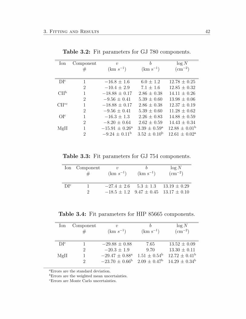
Table 3.2: Fit parameters for GJ 780 components.
Ion Component v b logN# (km s−1) (km s−1) (cm−2)
DIc 1 −16.8 ± 1.6 6.0 ± 1.2 12.78 ± 0.252 −10.4 ± 2.9 7.1 ± 1.6 12.85 ± 0.32
CIIb 1 −18.88 ± 0.17 2.86 ± 0.38 14.11 ± 0.262 −9.56 ± 0.41 5.39 ± 0.60 13.98 ± 0.06
CII∗c 1 −18.88 ± 0.17 2.86 ± 0.38 12.37 ± 0.192 −9.56 ± 0.41 5.39 ± 0.60 11.28 ± 0.62
OIc 1 −16.3 ± 1.3 2.26 ± 0.83 14.88 ± 0.592 −8.20 ± 0.64 2.62 ± 0.59 14.43 ± 0.34
MgII 1 −15.91 ± 0.26a 3.39 ± 0.59a 12.88 ± 0.01b
2 −9.24 ± 0.11b 3.52 ± 0.10b 12.61 ± 0.02a
Table 3.3: Fit parameters for GJ 754 components.
Ion Component v b logN# (km s−1) (km s−1) (cm−2)
DIc 1 −27.4 ± 2.6 5.3 ± 1.3 13.19 ± 0.292 −18.5 ± 1.2 9.47 ± 0.45 13.17 ± 0.10
Table 3.4: Fit parameters for HIP 85665 components.
Ion Component v b logN# (km s−1) (km s−1) (cm−2)
DIc 1 −29.88 ± 0.88 7.65 13.52 ± 0.092 −20.3 ± 1.9 9.70 13.30 ± 0.11
MgII 1 −29.47 ± 0.88a 1.51 ± 0.54b 12.72 ± 0.41b
2 −23.70 ± 0.66b 2.09 ± 0.47b 14.29 ± 0.34b
aErrors are the standard deviation.bErrors are the weighted mean uncertainties.cErrors are Monte Carlo uncertainties.
3. Fitting and Results 43
Overall, for GJ 780 and HIP 85665, we find consistent ISM velocities in each
different ion. We do note that they are not all the same as the MgII velocity, and
we present a discussion of these offsets in Section 3.4.1. In general, as expected,
the b values increase with decreasing atomic mass. HI and DI always have the
largest Doppler parameters because they are dominated by thermal broadening.
We see this same general result in our data. Additionally, our log column densities
are very similar to average values measured by Redfield & Linsky (2008).
3.4.1 Velocity Offsets
We note that the component velocities for each ion in GJ 780 are not all the
same as the MgII velocity, which we consider to be our baseline velocity. There
are several reasons for these offsets. First, deuterium absorption is almost always
very broad, which we can see in the high Doppler parameters. The uncertainties
on the DI velocities account for this in that they are fairly large. We performed a
quick test of the uncertainties by fitting the DI absorption with two components at
the MgII velocities of −15.9 km s−1 and −9.2 km s−1. The resulting fit was nearly
identical to the best-fit model with the above DI velocities. There only were slight
− within the 1σ errors of the other fit − changes to the Doppler parameters and
column densities, which was expected.
When we consider the seemingly too-high velocity resulting from the CII fit, we
also have to include consideration of the saturation in the line. Redfield & Linsky
(2004a) found an average Doppler parameter of 3.64 km s−1 in their survey of
stars within 100 pc that had high-resolution observations of interstellar FeII or
MgII. While we report Doppler parameter values of 2.86 ± 0.38 km s−1 and
5.39 ± 0.60 km s−1 that are on either side of the average value, we note that
3. Fitting and Results 44
Redfield & Linsky (2004a) also had a wide range of CII Doppler parameters. For
example, the η UMa CII spectrum showed evidence of strong saturation and, as
such, Redfield & Linsky (2004a) recorded Doppler value of 6.16 ± 0.71 km s−1.
Like the b value of our second component, this η UMa CII Doppler parameter
is systematically high due to saturation in the line. Therefore, we think our
higher radial velocity measurement is due to saturation. We also note that the
uncertainties on the CII velocities are probably too low. Therefore, if we had
reasonable uncertainties, we would likely consider the CII velocities to be within
3σ of the MgII velocities. Similarly, the difference between the OI component
velocities and the MgII velocities is also due to saturation, but on a less significant
scale.
We see similar offsets in the HIP 85665 velocities. However, we had to set the
DI Doppler widths at fixed values in order to get gismfit to construct an accurate
fit to the data. When left unconstrained, the Doppler parameters were slightly
too high even for deuterium. We do note that the second DI component velocity
is 1.8σ from its complementary MgII velocity and that this is not an unreasonable
difference due to the uncertainties on the DI velocities.
3.4.2 Geocoronal Features
The Earth’s atmosphere is constructed in layers, with the exosphere being the
outermost and most tenuous. The exosphere begins at an altitude of around 500
km, and has been detected out to ∼15.5 R (Schultz 2014). It is composed of
mostly neutral hydrogen atoms, and is detectable at UV wavelengths as a result of
interactions with high energy photons from the Sun. Typically, we see substantial
background emission due to HI. We often also detect absorption features in NI and

3. Fitting and Results 45
OI due to this terrestrial material (Redfield & Linsky 2004b). This absorption is
usually easily identifiable because it is centered at the mean velocity of the Earth
during the time of observation.
In the case of OI absorption in the GJ 780 spectrum, to yield a good fit to
the data and get appropriate values for physical parameters, we had to force the
OI b values to be at LISM average values. The b value of the second component
(at −9 km s−1) was chosen to be fixed at 3.24 km s−1, the average for the OI b
value (Redfield & Linsky 2004a). However, in order to get a Doppler parameter
that was physically probable, we had to also fix the Doppler parameter of the first
component at 6.70 km s−1. This value is substantially higher than the average, but
is not unprecedented given that Redfield & Linsky (2004a) measured a Doppler
parameter of 6.63 ± 2.99 km s−1 for ι Cap. When the Doppler parameters were
allowed to vary in order to reach the lowest possible χ2, as is the typical procedure
when fitting absorption components, the second component Doppler parameter
soared to the unphysical value of 8.2 ± 0.9. Though we determine a decent fit
to the data for the ISM absorption in OI, it was not ideal because of the fixed b
values.
However, we were able to produce a far more excellent fit to the GJ 780 OI
data when we included a geocoronal absorption feature. We used the IDL module
baryvel to calculate the barycentric velocity of the Earth at the time observations
of GJ 780 were taken with HST /STIS. baryvel outputs the barycentric velocity
components of Earth in a right-handed coordinate system with the positive x-
axis toward the Vernal Equinox and the positive z-axis pointed toward the North
Celestial Pole.1 Then, we projected the components of barycentric velocity along
the line of sight toward GJ 780 using the celestial coordinates of the star. This
1https://idlastro.gsfc.nasa.gov/ftp/pro/astro/baryvel.pro
3. Fitting and Results 46
gave the velocity (vr ≈ −19.8 km s−1) of the geocoronal component which was
seen as an emission feature in HI, and as an absorption feature in the members of
the OI multiplet. Once we had the velocity of the geocoronal component, we again
used gismfit to perform a fit to the OI absorption. Instead of two components,
like we used before, we included the geocoronal absorption as a third component
with velocity vr ≈ −19.8 km s−1. Adding the third component decreased the
Doppler parameters of the two ISM components to reasonable physical values
(2.26 ± 0.83 km s−1 and 2.62 ± 0.59 km s−1), and also resulted in the expected
ISM velocities that were consistent with the MgII fits.
In Figure 3.6, we present both the DI line and Lymanα line of HI for GJ 754
and HIP 85665. The geocoronal emission can clearly be seen at around 50 km s−1
as a distinct peak. In Figure 3.7, we present the OI multiplet for GJ 780 with the
geocoronal absorption feature velocity marked by the red line. ISM absorption is
only seen in the 1302 A line. We can distinguish between geocoronal absorption
and ISM absorption by looking at the other two lines of the multiplet. The OI 1304
A and 1306 A lines do not show any signs of ISM absorption, but the geocoronal
velocity matches up perfectly with an absorption feature. We also show in Figure
3.8 that the geocoronal velocity for GJ 780 lines up with the geocoronal emission
in HI.

3. Fitting and Results 47
Figure
3.6:
Pre
sente
din
the
figu
reab
ove
are
the
DI
lin
ean
dL
ym
anα
lin
eof
HI
for
bot
hG
J75
4an
dH
IP85
665.
Th
eb
lack
his
togra
mis
the
ob
serv
edfl
ux
data
plo
tted
inve
loci
tysp
ace,
scal
edby
the
centr
alw
avel
engt
hof
DI.
Th
eb
otto
max
isan
dti
cks
rep
rese
nt
the
vel
oci
tyof
DI,
an
dth
eto
pax
isan
dti
cks
are
the
velo
city
ofH
I.T
he
pea
kat∼
50km
s−1
isH
Iem
issi
onfr
omth
egeo
coro
na.
Th
eco
lore
dve
rtic
al
lin
esin
dic
ate
velo
citi
esof
the
LIS
Mcl
oud
sp
red
icte
dto
lie
wit
hin
10
ofth
est
ar(f
rom
Red
fiel
d&
Lin
sky
(2008
)).
Th
ere
dli
ne
isth
eM
iccl
oud
,b
lue
isth
eG
clou
d,
cyan
isth
eV
elcl
oud
,or
ange
isth
eA
ql
clou
d,
gree
nis
the
Op
hcl
oud
,an
dp
urp
leis
the
LIC
.

3. Fitting and Results 48
Figure
3.7:
Sam
eas
Fig
ure
3.6
,b
ut
show
ing
the
OI
mu
ltip
let
ofG
J78
0at
1302
,13
04,
and
1306
A.
Th
ere
dli
ne
isth
eve
loci
tyof
the
geoco
ron
al
com
pon
ent,
the
gree
nli
ne
isth
eve
loci
tyof
the
firs
tab
sorp
tion
com
pon
ent,
and
the
blu
eli
ne
isth
eve
loci
tyof
the
seco
nd
abso
rpti
on
com
pon
ent.

3. Fitting and Results 49
Figure 3.8: Same as Figure 3.6, but for the Lymanα line of HI.
3.5 The Lyman α Profile
The hydrogen Lyman α line is crucial to the study of solar and interstellar
dynamics. The line is the first in the Lyman series of transitions, occurring at
1215.6700 A. This wavelength is easily observed by HST /STIS, and we were there-
fore able to obtain high-resolution spectra of far-UV wavelength bands containing
both the HI and DI Lyα lines. Interstellar hydrogen and deuterium atoms pro-
duce absorption features against the stellar Lyα line profile (Wood et al. 2005).
These features are almost always strong enough to be observed for any sight
line because hydrogen is so abundant, and ultimately provide important informa-
tion about the LISM. Sometimes, in addition to the interstellar absorption, Lyα
spectra show signs of absorption from the outer heliosphere or even from other

3. Fitting and Results 50
astrospheres (Wood et al. 2005). An astrosphere is the same structure as our
heliosphere, but is one that occurs around other stars. The basic astrospheric
model designed by Linsky & Wood (2014) includes a termination shock where the
solar wind becomes subsonic, an astropause (analogous to the heliopause), and
a hydrogen wall (H-wall), where inflowing neutral hydrogen accumulates and is
heated by particle interactions. In the HI Lyα profile, the solar H-wall appears as
extra absorption red-ward of the LISM absorption, while a stellar H-wall would
appear blue-ward of the LISM absorption (Linsky & Wood 2014).
Before we can even model the missing stellar continuum, we have to remove
the geocoronal emission. Because the geocoronal emission is relatively narrow
and contained within the saturated core of HI, it can be approximated by fitting
a simple Gaussian profile with gismfit and then subtracting it out from the
data (Wood et al. 2005). The geocorona also can act as a wavelength calibrator.
The data reduction is done in a heliocentric rest frame, which means that the
geocoronal emission is at a velocity that is the projected barycentric velocity of
Earth at the same time. We can then compare the calculated baryvel velocity
with the actual emission line center and determine if an offset exists. In order to
determine the sources of absorption, we must first reconstruct the unknown stellar
emission line (Linsky & Wood 1996). This is particularly difficult to do because
the hydrogen Lyα line is broad and often saturated. We can see in Figure 3.4 that
the absorption in HI Lyα is indeed extremely broad − spanning at least 80 km s−1
in velocity space − and definitely saturated. The saturation stems from not only
the high abundance of neutral hydrogen atoms in the LISM, but also the high
oscillator strength of hydrogen. HI column densities even for short sight lines are
high enough that the absorption profile has extended damping wings (Wood et al.
2005). This just adds another level of complexity to the profile reconstruction, but

3. Fitting and Results 51
it just so happens that our fits to the DI Lyα line can provide initial conditions
for reconstructing the HI profile. The DI absorption fit should indicate what the
central wavelength and Doppler width would be for HI (Wood et al. 2005). The
HI absorption should have the same centroid velocity as deuterium, and the two
Doppler parameters are related by b(HI) ≈√
2b(DI). This equation allows us
to compute a Voigt opacity profile, τλ for HI based on various assumed values
for hydrogen column density (Wood et al. 2005). This profile can effectively
reconstruct the “wings” of the HI Lyα line when we multiply the data by exp(τλ).
To reconstruct the rest of the profile we consider the MgII h and k lines. Both
Lyα and the MgII doublet are optically thick chromospheric lines that have similar
profiles when seen in the solar spectrum (Wood et al. 2005). The stellar continua
for both MgII and Lyα will often be the same shape, and therefore we can use the
MgII lines to reconstruct the HI Lyα profile. The program lymangauss, written
by E. Edelman, uses a certain number of Gaussians to approximate the double-
peaked shape of the MgII lines and then places the new continuum over the center
of the Lyα line. In Figure 3.9, we present an initial reconstruction of the HI Lyα
in GJ 780. Note that this is a preliminary, reconstruction with the final fit to be
completed in the future.

3. Fitting and Results 52
Figure 3.9: Initial reconstruction of the HI Lyα profile in GJ 780. The black histogramis the observed flux data. The blue line is a simple Gaussian intended to represent themissing stellar continuum.

Chapter 4
Analysis of Physical Parameters
The ISM fit parameters can be used to measure the physical properties of
the LISM. We hope that these physical constraints will allow us to identify the
interstellar clouds that are the sources of the absorption we see. Ultimately,
we want to characterize the LISM through which the Voyager spacecraft will
eventually travel and connect our derived measurements to those measured in
situ by the spacecraft.
4.1 Comparing with the Kinematic Model
In Section 3.4, we presented our calculated radial velocity values for each of
the ISM absorption components for three sight lines. We now include in greater
detail a discussion of how well our velocities match known LISM cloud velocities.
Redfield & Linsky (2008) provide an online LISM Dynamical Model Kinematic
Calculator,1 which calculates which LISM clouds are traversed for any sight line
given the coordinates of that sight line. The Kinematic Calculator also calcu-
lates the radial and transverse velocities for each of the 15 clouds in the model
developed by Redfield & Linsky (2008). In the following table, we present a com-
parison between our radial velocities and those from the Kinematic Calculator.
1http://lism.wesleyan.edu/LISMdynamics.html

4. Analysis of Physical Parameters 54
Tab
le4.1
:C
omp
aris
onw
ith
LIS
MD
yn
amic
alM
od
el.
Glies
eO
ther
Dis
tance
Com
pon
ent
vC
loud
Alt
ernat
ive
#N
ame
(pc)
#(k
ms−
1)
Expla
nat
ion
Voy
ager
1G
J67
8.1A
aH
IP85
665
9.98
1−
29.6
8±
0.62
cO
ph
2−
23.4±
2.4b
LIC
Voy
ager
2G
J78
0aδ
Pav
6.11
1−
18.0±
1.3b
Vel
2−
9.23±
0.90
bD
orG
J75
4L
HS
605.
911
−27
.4±
2.6d
Vel
G,
Mic
(?)
2−
18.5±
1.2d
GA
ql(
?)
aV
eloci
tyis
the
wei
ghte
dm
ean
ofth
evel
oci
ties
fou
nd
for
each
ion
.bE
rror
sar
eth
est
and
ard
dev
iati
on.
cE
rror
sar
eth
ew
eigh
ted
mea
nu
nce
rtai
nti
es.
dE
rror
sar
eM
onte
Car
lou
nce
rtai
nti
es.

4. Analysis of Physical Parameters 55
One important feature of the Kinematic Calculator is that it not only returns
the projected velocity vectors for all 15 clouds, but also lists which clouds are tra-
versed by the sight line, which clouds are within <20 of the sight line, and which
clouds are far (>20) from the sight line. We were able to predict which clouds cor-
respond to each ISM absorption component based off the both the velocity vectors
and if a cloud traverses the sight line or not. If more than one cloud is a possible
match to the component velocity, it is listed under “Alternative Explanation.”
4.1.1 The Voyager 1 Sight Line
Though we only were able to calculate velocities for one target star along the
Voyager 1 sight line, we actually find that these velocities match up quite well
with known ISM cloud velocities. HIP 85665 has the smallest angular separation
∆θ from the Voyager 1 sight line, indicating a strong likelihood that whatever
clouds we identify along its path will intersect with the path of Voyager 1. The
first absorption component has a velocity of −29.68 ± 0.62 km s−1, which is nearly
identical to the predicted velocity for the Oph cloud (vr = −29.66 ± 0.64 km s−1).
Therefore, we are confident that we see absorption from the Oph cloud along the
Voyager 1 line of sight.
The second component is slightly more ambiguous. The averaged velocity of
−23.4 ± 2.4 km s−1 is only 0.5σ away of the velocity of the LIC cloud, which is
−22.15 ± 0.99 km s−1. However, we note that the higher velocity could indicate
contamination from other clouds that traverse the Voyager 1 sight line to HIP
85665. The Mic cloud is also traversed by this sight line, and it has a velocity of
−27.05 ± 0.98 km s−1. The G cloud falls within 20 of this line of sight, and also
has a velocity around −27 km s−1. It is entirely possible that we see some minor
4. Analysis of Physical Parameters 56
absorption from one or both of these two nearby clouds. However, we believe that
the component velocity matches up well with the LIC.
4.1.2 The Voyager 2 Sight Line
Unlike the Voyager 1 sight line, the Voyager 2 sight line is a bit more com-
plicated. We have absorption component velocities for both target stars − GJ
754 and GJ 780 − but the uncertainty on the GJ 754 component velocities are
considerably higher than those of GJ 780. We were only able to detect ISM ab-
sorption in DI, and as such, the constraints on the velocity values are looser than
those determined by examining the MgII doublet. Despite falling within 15 of the
direct Voyager 2 line of sight, GJ 780 and GJ 754 are actually greater than 20
away from each other. This large distance discrepancy between the two targets
lends some uncertainty to which clouds occur on the path of Voyager 2.
With a velocity of −18.0 ± 1.3 km s−1, the first component of GJ 780 matches
up closely with the velocity of the Vel cloud (vr = −18.71 ± 1.09 km s−1). Ac-
cording to the Kinematic Calculator, the Voyager 2 sight line to GJ 780 directly
traverses the Vel cloud. The other clouds to which the sight line passes near all
have velocities that could not sufficiently explain the velocity measured for the
first absorption component. The discrepancy between the measured velocity and
the Kinematic Calculator-based velocity is is not larger than either of the asso-
ciated uncertainties. We therefore are confident that we see absorption from the
Vel cloud in the first component of GJ 780.
The second observed absorption component of GJ 780 also appears to nearly
match with an identified cloud. The Kinematic Calculator indicates that the Dor
cloud passes near (<20) the Voyager 2 line of sight with a velocity of −8.62 ±

4. Analysis of Physical Parameters 57
0.60 km s−1. We find that the second component has a velocity of −9.23 ± 0.90
km s−1. This component velocity is consistent with the velocity of the Dor cloud
to <1σ, which indicates that it is a good match.
The velocities of the two components of GJ 754 are more difficult to match with
known ISM clouds. Not only are the uncertainties higher, but also the absorption
we see could be from more than one cloud. The Voyager 2 sight line to GJ 754
directly traverses the Aql cloud and passes within 20 of the G, Mic, and Vel
clouds. However, though the first component’s velocity of −27.4 ± 2.6 km s−1 is
not consistent with the Aql cloud velocity, it is only 1.5σ away from that of the Vel
cloud (vr = −31.89 ± 1.52 km s−1). That the first absorption component velocity
is lower than the velocity of the Vel cloud could indicate contaminant absorption
by the G or Mic clouds (vr = −20.55 ± 1.51 km s−1 and vr = −21.68 ± 1.19 km
s−1, respectively). It is more likely that the velocities of both the first and second
absorption components would be better constrained if we had ISM absorption in
the Mg II h and k lines. Because we do not, the values from absorption in DI are
fairly ambiguous.
Similarly, the second component of GJ 754 has a velocity of −18.5 ± 1.2 km
s−1, which is in between the velocities of the G and Aql clouds. It falls about
1.9σ away from the velocity of the G cloud, indicating that the G cloud is likely
a primary source of the observed absorption. We cannot definitively rule out that
we see some absorption from the Aql cloud because it lies directly along the line
of sight to GJ 754.

4. Analysis of Physical Parameters 58
4.2 Temperature and Turbulence
Since we have measurements of Doppler parameters resulting from the fits, we
can derive estimates for temperature and turbulence of the ISM along the lines of
sight. The equation that illustrates the relationship between Doppler parameter
(b [km s−1]), temperature (T [K]), and turbulent velocity (ξ [km s−1]) is
b2 =2kT
m+ ξ2 = 0.01662
T
A+ ξ2, (4.1)
where k is the Boltzmann constant, m is the mass of the observed ion, and A
is the atomic weight of the element (Redfield & Linsky 2004b). It is possible
to solve Equation 4.1 for temperature and turbulence with only two line width
components. However, the two ions must have very different atomic weights in
order for this to yield accurate measurements (Redfield & Linsky 2004b). While it
would be best to use the two ions that have the greatest mass difference, hydrogen
and iron, we do not have any value on the Doppler parameter for any iron lines.
Instead, MgII can be used as a proxy for iron because it is the next heaviest
commonly detected ion. For GJ 780, we have, for both absorption components,
four different ions − MgII, CII, OI, and DI − we can use. DI is the next lightest
ion after HI and is typically unsaturated for short sight lines, therefore providing
a reliable Doppler parameter for measurement (Redfield & Linsky 2004b).
We present four plots, Figures 4.1-4.4, for GJ 780 and HIP 85665 visualizing
the temperature and turbulent velocity determination. The values and associated
uncertainties were calculated and then plotted using the IDL routine plot temp.
We also present, in Table 4.2, both the parameters that were used to calculate
temperature and turbulence and the results from the calculated values.

4. Analysis of Physical Parameters 59
Figure 4.1: The left-side plot shows temperature versus turbulent velocity for a givenDoppler parameter of a particular ion. The colors indicate the ion. For example:deuterium is red, carbon is purple, oxygen is blue, and magnesium is green. The coloreddashed lines are ±1σ errors around the solid line, which is from Equation 4.1, yieldingan individual best-fit curve in the temperature-turbulence plane (Redfield & Linsky2004b). The black cross is the best-fit value of the temperature and turbulent velocitybased on the measured Doppler parameters. The black contours are 1 and 2σ errors forboth values (Redfield & Linsky 2004b). The right-side plot shows Doppler parameterplotted against the atomic mass of the ions. The red symbols are the observed Dopplerparameter values and associated uncertainties from the data. The solid line is the best-fit curve given from Equation 4.1. The shaded region includes all fits within the 1σcontours from the left-side plot.

4. Analysis of Physical Parameters 60
Figure 4.2: Same as Figure 4.1, but for the −9 km s−1 component of GJ 780.
Figure 4.3: Same as Figure 4.1, but for the −29 km s−1 component of HIP 85665without carbon or oxygen.
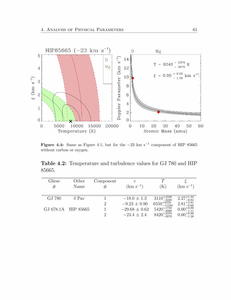
4. Analysis of Physical Parameters 61
Figure 4.4: Same as Figure 4.1, but for the −23 km s−1 component of HIP 85665without carbon or oxygen.
Table 4.2: Temperature and turbulence values for GJ 780 and HIP85665.
Gliese Other Component v T ξ# Name # (km s−1) (K) (km s−1)
GJ 780 δ Pav 1 −18.0 ± 1.3 3110+2430−3220 2.27+1.44
−0.84
2 −9.23 ± 0.90 6550+6550−11550 2.81+2.81
−0.66
GJ 678.1A HIP 85665 1 −29.68 ± 0.62 5420+1750−2090 0.00+0.00
−1.11
2 −23.4 ± 2.4 8420+2370−2670 0.00+0.00
−1.26
4. Analysis of Physical Parameters 62
Now that we have identified the most likely ISM clouds from which we measure
the velocities of absorption components, we can begin to make comparisons be-
tween our derived temperatures and turbulences and the averaged measurements
for specific clouds calculated by Redfield & Linsky (2008).
We are confident that we see absorption in the two components along the Voy-
ager 2 line of sight (GJ 780) from the Vel and Dor clouds, respectively. Redfield
& Linsky (2008) do note that there was only one sight line with physical mea-
surements for each cloud, and that their measured values are uncertain. We are
confident in our measurement for the temperature and turbulence of the Vel cloud
after adjusting the OI fit to include the geocoronal absorption component. We find
a temperature of 3110+2430−3220 K and a turbulence of 2.27+1.44
−0.84 km s−1. Our temper-
ature is vastly different than what was derived by Redfield & Linsky (2008), but
this discrepancy between our measured temperature and the Redfield & Linsky
(2008) temperature of 10600 K is due to the uncertainty in their measurement.
With further measurements along additional Vel lines-of-sight, we could certainly
better constrain the temperature. Their turbulence (ξ = 3.5 km s−1) is 0.85σ
from our value. Again, additional observations would be necessary to tighten the
uncertainties and solidify the average value for Vel.
The second component, which we identify as the Dor cloud, has a temperature
of 6550+6550−11550 K, which is very close to the Redfield & Linsky (2008) temperature of
7000K. However, we have to consider that the error bars on the second component
temperature are extremely large. We acknowledge that the below-zero lower limit
is likely an artifact of the fitting routine, and should not be considered to be a
real temperature value. Likewise, the turbulence we find (ξ = 2.81+2.81−0.66 km s−1)
is 0.95σ from the average Dor turbulence of 5.5 km s−1. However, we can see
from the left-side panel in Figure 4.2 that the CII and OI best-fit curves to the
4. Analysis of Physical Parameters 63
temperature-turbulence plane to not match up well with the best-fit value. This is
likely because the absorption components were saturated, and we could not obtain
an entirely accurate estimate the respective Doppler parameters. However, we do
see that the Doppler parameters for both CII and OI are reasonably close to the
best-fit curve plotted in the right-side panel of Figure 4.2.
While the temperatures of the two HIP 85665 components are reasonable,
the turbulence values are somewhat unrealistic. Both turbulences have a best-
fit value of 0 km s−1. We can see from Figures 4.3 and 4.4 that the 1 and
2σ contours indicate the possibility of having positive turbulence. A probable
cause for the turbulence values being what they are is that we only have two
Doppler parameter values available for fitting. This likely reduces the certainty
with which we can constrain our additional physical parameters. We are confident
in our conclusion made in Section 4.1 that we see absorption from the Oph and
LIC clouds in our first and second absorption components, respectively. However,
the average turbulences (ξOph = 3.3 km s−1 and ξLIC = 1.62 ± 0.75 km s−1) are
nowhere near the values we derive. Despite the large discrepancies in turbulence,
the temperature values for both components match up reasonably well with their
respective averages from Redfield & Linsky (2008). Like the Vel and Dor clouds,
the Oph cloud only has one line of sight for which physical measurements could
be made (Redfield & Linsky 2008). We take this uncertainty into account, and
therefore find that our temperature of 5420+1750−2090 K is reasonable for the Oph
cloud. Luckily, Redfield & Linsky (2008) have 79 total sight lines for the LIC,
with 19 of those used to calculate an average temperature of 7500 ± 1300 K. Our
temperature value of 8240+2370−2670 K is similar to temperatures measured along other
LIC sight lines, and is relatively close to the average temperature. Based on the
wide range of LIC temperatures, we conclude that our temperature coincides well

4. Analysis of Physical Parameters 64
with other LIC sight line temperatures.
4.3 Abundance and Depletion
As previously discussed in Section 1.3.3, depletion occurs when heavy elements
have gas phase abundances that are less than the expected cosmic abundances,
presumably due to incorporation into dust. Depletion is calculated from
log(Xgas/H) = log(N(X)/N(H))− log(X/H), (4.2)
where X denotes the heavier element, N(X) is the column density of that ele-
ment, and H is hydrogen (Jenkins 2009). Equation 4.2 indicates that the deple-
tion is determined by first calculating the ISM abundances and then subtract-
ing the solar abundances (Wood et al. 2002). Hydrogen abundance is calcu-
lated from the deuterium column density and then converted to hydrogen by us-
ing a deuterium-to-hydrogen ratio (hereafter, D/H) (Redfield & Linsky 2008).
The most accurate LISM D/H ratio was calculated by Linsky et al. (2006),
who used measurements of D/H from the Far Ultraviolet Spectroscopic Explorer
(FUSE ), HST, Copernicus, and the Interstellar Medium Absorption Profile Satel-
lite (IMAPS ). They determined that the D/H ratio of (1.56 ± 0.4)×10−6 is con-
sistent for column densities log[N(H)]<19.2. This column density is indicative
of ISM inside the Local Bubble. Because all four of our target stars are within
20 pc of Earth, they lie well within the edge of the Local Bubble (∼50 pc).
As suchm we use the Linsky et al. (2006) D/H ratio to convert from N(DI) to
N(H). We also adopt solar abundances and the associated uncertainties from
Asplund et al. (2009). The error on the results from Equation 4.2 was calcu-
lated by error propagation based on the uncertainties on logN(X) and logX.

4. Analysis of Physical Parameters 65
We present in Table 4.3 gas and dust depletions for MgII, CII, and OI in GJ
780, and in Table 4.3 MgII depletion toward HIP 85665. The “X” in the header
of each table denotes the respective element according to the Ion column.
The most notable result from these calculations is that most of these ions
appear to be locked in dust - that is, their respective abundances are high for
dust and low for gas. We see that the dust column densities are higher than the
gas column densities given in Tables 3.2−3.4. Like in Section 4.2, we can also make
a general comparison to depletion values calculated by Redfield & Linsky (2008).
We see absorption from two component clouds, Vel and Dor, along the GJ 780
sight line. Unfortunately, we find that neither of our magnesium depletion values
(−1.30 ± 0.004 and −1.65 ± 0.004, respectively) match up with those measured
by Redfield & Linsky (2008) along the Vel and Dor lines of sight. However,
just as mentioned in Section 4.2, we keep in mind that their values are highly
uncertain. We find that their depletions for both clouds − 〈D(Mg)〉Vel = −0.03
and 〈D(Mg)〉Dor = −0.65 − are significantly different from our depletions.
Likewise, the magnesium depletion of the first component in HIP 85665, from
the Oph cloud, does not match up at all with the measurement from Redfield &
Linsky (2008). Again, Redfield & Linsky (2008) only had one sight line with phys-
ical measurements for the Oph cloud, but regardless, our value of −2.206± 0.004
is nowhere near their measurement of −0.84± 0.34. It is entirely possible that we
are seeing a different part of the cloud than was observed by Redfield & Linsky
(2008), but without further confirmation from other physical measurements, we
cannot definitively conclude on this comparison. However, the magnesium de-
pletion of the second component from the LIC matches up reasonably well with
the average value from Redfield & Linsky (2008). Our value of −0.423± 0.004 is

4. Analysis of Physical Parameters 66
Tab
le4.3
:G
J78
0an
dH
IP85
665
dep
leti
onva
lues
.
Ion
Com
pon
ent
logN
(X) g
as
logN
(H)
logX
a
logX
gas/
Hlo
gN
(X) d
ust
#(l
ogcm
−2)
(log
cm−
2)
(log
cm−
2)
GJ
780
CII
114
.11±
0.26
18.5
9±
0.25
8.43±
0.05
−0.
88±
0.01
14.9
6±
0.25
213
.98±
0.06
18.6
6±
0.32
...
−1.
11±
0.01
15.0
5±
0.32
OI
114
.62±
0.14
18.5
9±
0.25
8.69±
0.05
−0.
65±
0.01
15.1
7±
0.25
214
.03±
0.57
18.6
6±
0.32
...
−1.
32±
0.01
15.3
3±
0.32
MgI
I1
12.8
8±
0.01
18.5
9±
0.25
7.60±
0.04
−1.
30±
0.00
414
.16±
0.25
212
.61±
0.02
18.6
6±
0.32
...
−1.
65±
0.00
414
.25±
0.32
HIP
8566
5M
gII
112
.72±
0.41
19.3
3±
0.09
7.60±
0.04−
2.20
6±
0.00
414
.93±
0.10
214
.29±
0.34
19.1
1±
0.11
...
−0.
423±
0.00
414
.50±
0.11
aW
her
elo
gH
=
12

4. Analysis of Physical Parameters 67
at the lower edge compared to the range of values the authors measured for the
LIC. It happens that our depletion is 2.4σ from their average of −0.97 ± 0.23.
A possible explanation for this slightly lower magnesium depletion is the sheer
size of the LIC. It covers approximately 18300 deg2 across the sky, which is an
extremely vast area compared to other ISM clouds (see Figure 1.5). The fact that
the LIC is so large may allows for such discrepancies between individual sight line
measurements.
4.4 Electron Density
One of the most important measurements we were able to make was to derive
a value for electron density along the Voyager 2 sight line. Because both Voyager
spacecraft are still capable of measuring electron density with the Plasma Wave
System2, we can compare our derived electron density value with their in situ
measurements. Redfield & Falcon (2008) measured electron densities (ne) using
the ratio of the collisionally excited CII line column density to the resonance CII
line column density. The excited carbon line is a fine-structure doublet. Fine-
structure describes how spectral lines of atoms split into degenerate multiplets
from relativistic corrections leading to a small shift in energy on the order of
10−4− 10−5eV. The presence of these fine structure lines in the ISM gives density
information of the absorbing medium (Bahcall & Wolf 1968). Densities derived
from the collisionally excited lines do not depend on the radiation field, which is
why they are used (Frisch et al. 2011). The resonance absorption line at 1334.5323
A corresponds to the transition from the ground state at J = 12, while the CII
excited absorption line doublet (1335.6627 and 1335.7077 A) represents the tran-
2https://nssdc.gsfc.nasa.gov/nmc/experimentDisplay.do?id=1977-084A-13
4. Analysis of Physical Parameters 68
sition from the excited state of the fine-structure doublet at J = 32
(Bahcall & Wolf
1968; Redfield & Falcon 2008). Electron collisions are responsible for populating
the excited state, and therefore, the ratio of the column densities is proportional
to the electron density by
N(CII∗)
N(CII)=neC12(T )
A21
. (4.3)
The relation given in Equation 4.3 is derived from thermal equilibrium between
collisional excitation of the fine-structure doublet and total radiative de-excitation
(Redfield & Falcon 2008). In Equation 4.3, N(CII∗) and N(CII) are the column
densities of the excited line and resonance line, respectively, and A21 = 2.29 ×
10−6s−1 is the radiative de-excitation rate coefficient (Nussbaumer & Storey 1981).
The collision rate coefficient C12(T ) can be written as
C21(T ) =8.63× 10⁻⁶Ω12
g1T 0.5exp
(− E12
kT
), (4.4)
where g1 = 2 is the statistical weight of the ground state and E12 = 1.31× 10⁻¹⁴
ergs is the energy of the transition. Like Redfield & Falcon (2008), we adopt the
value of Ω12 = 2.81, and initially assumed a temperature of T = 7000 K.
We were fortunate in that the GJ 780 spectra contained ISM absorption in
CII and collisionally excited CII∗. We followed the fitting procedure outlined
by Redfield & Falcon (2008), but we were unable to perform an individual fit
to the excited line alone. The ISM absorption in CII∗ was present, but proved
exceedingly difficult to fit on its own. Instead, we performed a fit to the resonance
line, and then recreated the missing stellar flux for the excited line before finally
performing a simultaneous fit to both lines. We were able to successfully fit to

4. Analysis of Physical Parameters 69
both lines, and find well-constrained values for column density. We note that
the dominant source of systematic error comes from the saturation of the CII
resonance line, which is indicated by the high (∼5 km s−1) Doppler parameter of
the second ISM component (see Table 3.2). This saturation results from high CII
abundances and a high atomic oscillator strength (Frisch et al. 2011).
Using Equations 4.3 and 4.4, we were able to derive values for electron density
for both ISM absorption components in GJ 780. These values are presented in
Table 4.5. Table 4.5 not only includes the ne values for the initial temperature of
T = 7000 K, but also values for ne using the upper limits and median values for the
temperatures calculated in Section 4.2. The uncertainties on ne were calculated
using simple rules of error propagation based on the initial uncertainties on the
column densities. In particular, we note that the different temperatures do not
change the electron density by much.
Table 4.4: GJ 780 electron densities.
Component v logN(CII∗) logN(CII) T ne# (km s−1) (cm−2) (cm−2) (K) (cm−3)
1 −18.0 ± 1.3 12.37 ± 0.19 14.11 ± 0.26 7000 0.29 ± 0.21... ... ... 3110 0.20 ± 0.15... ... ... 5540 0.26 ± 0.19
2 −9.23 ± 0.90 11.28 ± 0.62 13.98 ± 0.06 7000 0.03 ± 0.05... ... ... 6550 0.03 ± 0.04... ... ... 13100 0.04 ± 0.06

4. Analysis of Physical Parameters 70
4.4.1 Comparisons to Voyager
In April 2013, shortly after it crossed the heliopause, Voyager 1 ’s Plasma Wave
System detected locally-generated electron plasma oscillations at a frequency of
about 2.6 kHz (Gurnett et al. 2013). Electron plasma oscillations occur at the
electron plasma frequency, a characteristic frequency of
fp = 8980√ne, (4.5)
where frequency has units of Hertz. The oscillations are excited by electron beams
such as those upstream of interplanetary or interstellar shocks or after energetic
solar outbursts (Gurnett et al. 2013). The Voyager spacecraft last observed elec-
tron plasma oscillations in 2004 (V1 ) and 2007 (V2 ) when just upstream of the
heliospheric termination shock. Gurnett et al. (2013) obtained a series of short
samples of the electric field waveform and used Fourier analysis techniques to
convert the waveforms into frequency-time spectrograms, as shown in Figure 4.5.
Using Equation 4.5, Gurnett et al. (2013) calculated that the frequency of 2.6
kHz corresponded to an electron density of ne = 0.08cm−3. Gurnett et al. (2013)
also discovered that the densities observed by Voyager 1 are gradually increasing
with radial distance at about 19% per AU. The observed electron densities are well
within the range of remote-sensing measurements of plasma densities (0.06−0.21
cm−3) in the LISM (Redfield & Falcon 2008). Based on Voyager 2 Plasma Wave
System measurements out to ∼100 AU, the electron densities in the heliosheath
(∼0.001−0.003 cm−3) are an order of magnitude smaller than those in the LISM
(Gurnett et al. 2013).
Our measurements of electron density for the Voyager 2 line of sight to GJ

4. Analysis of Physical Parameters 71
Figure 4.5: A composite spectrogram from Gurnett et al. (2013) that was constructedfrom spectrograms extending over a 1 year period. Electron density is given in theright-side axis. The vertical dashed white line denotes an increase in galactic cosmicrays in August 2012. The sloping dashed line indicates a density increase in the regionbetween the two marked plasma oscillation events corresponding to an increase of about19% per AU (Gurnett et al. 2013).
4. Analysis of Physical Parameters 72
780 clearly indicate the presence of the LISM. The first absorption component,
for temperatures between 3110−7000 K, has electron densities between 0.2−0.3
cm−3. Including uncertainties, the electron densities have a total range of 0.05−0.5
cm−3. These values are certainly a factor of three or greater than that measured by
Voyager 1, but are fairly consistent with previous predictions for electron density
in the LISM. The higher densities could suggest the presence of a high-density
ISM cloud. Based on our initial comparison to the Redfield & Linsky (2008)
Kinematic Model, we can be confident that these higher electron density values
confirm the presence of the Vel cloud.
The second absorption component has electron density values between 0.03−0.04
cm−3, which are a factor of three smaller than that measured by Voyager 1, but
still a full order of magnitude greater than the heliosheath electron density. How-
ever, when we calculate an upper limit from the uncertainties, the electron densi-
ties range between 0.07−0.1 cm−3, which is both exactly what was measured by
Voyager 1 and predicted by Frisch et al. (2011). Since we believe we see absorp-
tion from the Dor cloud, we can conclude that this cloud is less dense than the
Vel cloud. Once Voyager 2 crosses the heliopause within the next five years and
obtains new measurements of electron density, we will be able to better compare
its measurements with our derived values for electron density.
Chapter 5
Conclusions and Future Work
In June 2016, NASA extended the Hubble Space Telescope Science Operations
contract to 2021 in the hopes that the telescope would continue to operate until
at least 2020.1 Because it is in low-Earth orbit, HST experiences atmospheric
drag, and is slowly being pulled back down to Earth. Current estimates on when
Hubble will succumb to this drag force are sometime between 2030 and 2040. At
this point, it is unclear whether or not HST will continue to operate during the
2020s until its inevitable destruction. Until then, we can still obtain valuable
science data from the telescope. Even with the advent of the James Webb Space
Telescope era, there is no direct successor to Hubble as an ultraviolet and optical
space telescope.
Likewise, the Voyager spacecraft are expected to fully lose all operational
power by 2025,2 and will begin to quietly drift through interstellar space. Between
the two of them, the Voyagers not only explored all four outer planets − Jupiter,
Saturn, Uranus, and Neptune − but also investigated 48 moons and the rings
and magnetic field systems unique to each planet.3 Spacecraft that were initially
built to last only five years have completely exceeded all expectations. When the
Voyagers do lose power, they will have been traveling for nearly 50 years.
1https://www.nasa.gov/press-release/nasa-extends-hubble-space-telescope-science-operations-contract
2http://voyager.jpl.nasa.gov/spacecraft/spacecraftlife.html3http://voyager.jpl.nasa.gov/mission/fastfacts.html

5. Conclusions and Future Work 74
5.1 Future Work
There are several new analyses that can be done to further characterize the
LISM near the Voyager spacecraft. For example, while complicated, the HI profile
contains a substantial amount of information. We can fit the HI absorption by
performing a simultaneous fit to both DI and HI absorption. This process follows
the same steps as detailed in Section 3, but with a few extra components. In order
to better constrain the hydrogen absorption, we fix the centroid velocities of both
DI and HI to be equal to each other and utilize the equation, b(HI) ≈√
2b(DI),
to set the Doppler parameter widths (Wood et al. 2005). After the first initial
run of gismfit, the assumed stellar profile (which we presented in Section 3) is
altered to refine the overall fit. Since we have assumed the Linsky et al. (2006)
D/H value, we can use this to better constrain the HI fit parameters by relating
DI to HI. Ultimately, the HI absorption profile becomes more tightly constrained
even in the presence of multiple ISM absorption components (Wood et al. 2005).
Figure 5.2 shows the Wood et al. (2005) reconstruction of the stellar Lyα
emission line for their target ζ Boo. Each different profile assumes a different
column density (between logN(HI) = 17.6−18.2). Outside the dashed lines, the
profile is estimated based on the assumed logN(HI), while inside the dashed lines
shape is estimated from the shapes of the MgII h and k lines.
Presented in Table 5.1 are the parameters necessary for fully reconstructing
the Lyα line of HI in three of four target stars. We will use these column densities,
Doppler parameters, and velocities to define the shape of the Lyα continuum emis-
sion in the same way as Wood et al. (2005) did. We only list the DI ISM velocities
because the HI velocities will be the same. The errors on the HI column densities
and b values result from simple error propagation calculations. These parameters

5. Conclusions and Future Work 75
Figure 5.1: A reconstruction of the stellar Lyα line for ζ Boo from Wood et al. (2005).

5. Conclusions and Future Work 76
Tab
le5.1
:P
aram
eter
sfo
rfu
ture
reco
nst
ruct
ion
ofth
eH
IL
ym
anα
lin
esof
HIP
8566
5,G
J78
0,an
dG
J75
4.
Glies
eO
ther
Com
pon
ent
v DI
b DI
b HI
logN
(DI)
logN
(HI)
#N
ame
#(k
ms−
1)
(km
s−1)
(km
s−1)
(log
cm−
2)
(log
cm−
2)
Voy
ager
1G
J67
8.1A
HIP
8566
51
−29
.88±
0.88
7.65
10.8
213
.52±
0.09
19.3
3±
0.09
2−
20.3±
1.9
9.70
13.7
213
.30±
0.11
19.1
1±
0.11
Voy
ager
2G
J78
0δ
Pav
1−
16.8±
1.6
6.0±
1.2
8.5±
1.7
12.7
8±
0.25
18.5
9±
0.25
2−
10.4±
2.9
7.1±
1.6
10.1±
2.2
12.8
5±
0.32
18.6
6±
0.32
GJ
754
LH
S60
1−
27.4±
2.6
5.3±
1.3
7.4±
1.8
13.1
9±
0.29
19.0
0±
0.29
2−
18.5±
1.2
9.47±
0.45
13.3
9±
0.64
13.1
7±
0.10
18.9
8±
0.10

5. Conclusions and Future Work 77
will be especially important in reconstructing the “wings” of the profile, which we
did not do particularly well in the preliminary reconstruction (shown in Figure
3.9). We can see in Figure 5.2 that the amplitude of the Wood et al. (2005) Lyα
profile shifts with increasing column density. We predict that the same will apply
to our reconstructions. Additionally, we have not yet removed the DI absorption
from our Lyα flux data like Wood et al. (2005) did, but we plan on doing so in
order for this reconstruction to work. Ultimately, creating and estimating the
Lyman α line of HI is tricky business.
Future work may also include acquiring more data on the same targets and
looking for new targets. We could obtain more near-UV data with wavelength
ranges that include more observable resonance lines. GJ 780 in particular would
be a good follow-up target because our current observations yield a high S/N,
which would likely be reflected in any subsequent observations. Deviating more
than 15 from the Voyager sight lines would not characterize their future paths
as well, but it would be possible to better characterize that general area of LISM.
More distant targets have the disadvantage of being subject to blending, but would
help confirm or solidify the results we present in this work.
If we were to acquire more data on the same target stars as used in this work,
we could potentially try to obtain a measurement of optical polarization. Polar-
ization has been used to measure the structure of the Local Bubble for column
densities N(H)>1019.8 cm−2 or distances <40 pc (Frisch et al. 2011). Frisch et al.
(2010) obtained interstellar polarization observations of 30 nearby stars within
90 of the heliosphere nose to find the best fits to the polarization position angles.
They then compared their results with data from IBEX, and found that there was
similarity between the polarization direction and that of the IBEX Ribbon for the
interstellar magnetic field (ISMF). The IBEX Ribbon is a band of high energy
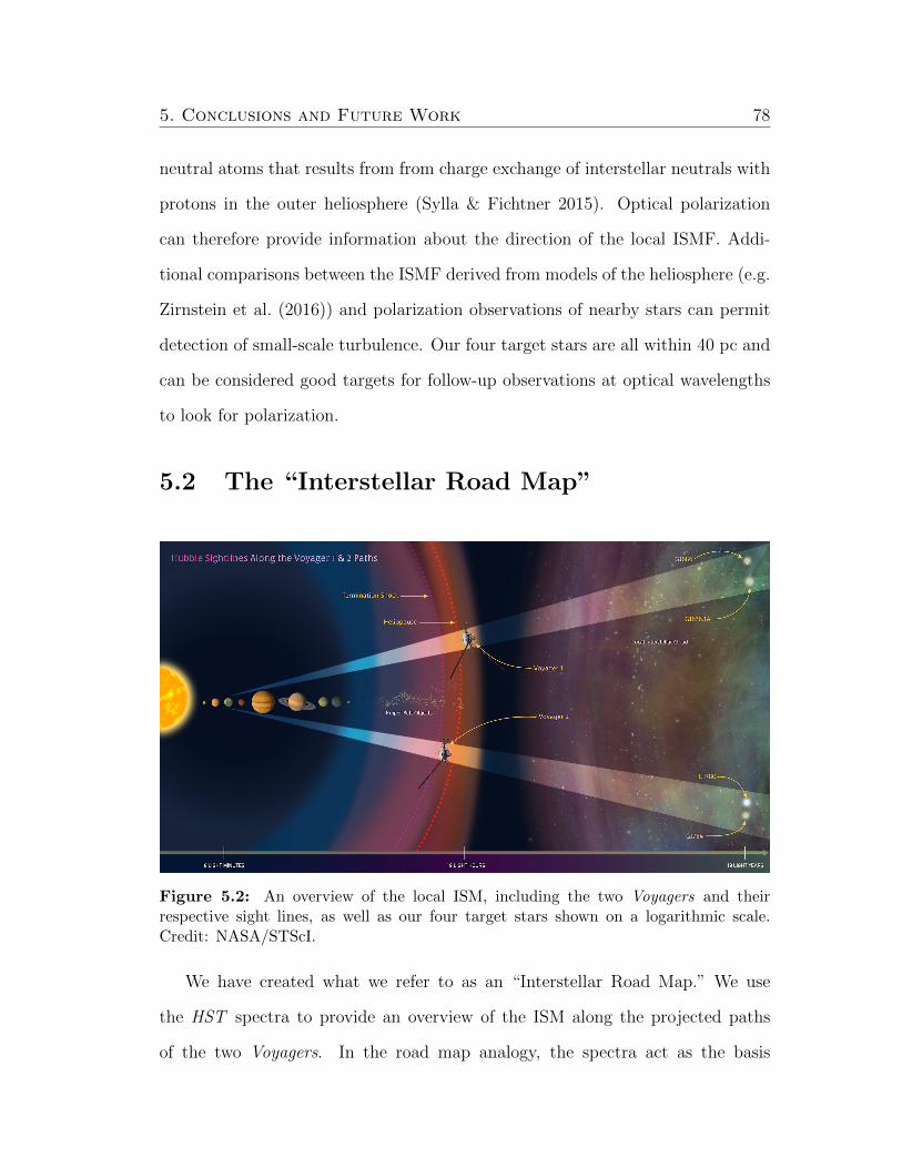
5. Conclusions and Future Work 78
neutral atoms that results from from charge exchange of interstellar neutrals with
protons in the outer heliosphere (Sylla & Fichtner 2015). Optical polarization
can therefore provide information about the direction of the local ISMF. Addi-
tional comparisons between the ISMF derived from models of the heliosphere (e.g.
Zirnstein et al. (2016)) and polarization observations of nearby stars can permit
detection of small-scale turbulence. Our four target stars are all within 40 pc and
can be considered good targets for follow-up observations at optical wavelengths
to look for polarization.
5.2 The “Interstellar Road Map”
Figure 5.2: An overview of the local ISM, including the two Voyagers and theirrespective sight lines, as well as our four target stars shown on a logarithmic scale.Credit: NASA/STScI.
We have created what we refer to as an “Interstellar Road Map.” We use
the HST spectra to provide an overview of the ISM along the projected paths
of the two Voyagers. In the road map analogy, the spectra act as the basis

5. Conclusions and Future Work 79
for the map, providing a general idea of what lies along the path ahead. The
Voyagers themselves act as the “street view,” sending us valuable measurements
of specific local physical properties. The one caveat is that the LISM is a dynamic
structure − it is constantly changing and evolving over time. Clouds that are
along the Voyager lines of sight now may not still be there when, in thousands of
years, the spacecraft reach the interstellar space we have probed with HST. Figure
5.1 visualizes how our observations directly connect to the Voyager spacecraft.
Though our target stars are not perfectly along the respective projected Voyager
lines of sight, they are all within 15 of it.
We have acquired high-resolution spectra along sight lines that canvass the
same ISM that the Voyager spacecraft are currently measuring, connecting two
of NASAs highly successful and enduring missions. We demonstrate that the
local ISM into which the Voyagers are moving is a complex and rich environment.
Though we observe the closest stars in those directions, we see multiple ISM
cloud absorbers. We definitively confirm the presence of known interstellar clouds,
including the Local Interstellar Cloud, in three of four sight lines. While some of
our comparisons to Redfield & Linsky (2008) do not match up with their derived
average values, Redfield & Linsky (2004b) note that variations in temperature and
turbulent velocity are common throughout the LISM. This presents the future
opportunity to refine the LISM Dynamical Model in the directions of our sight
lines. Ultimately, though, we were still able to consider the physical properties of
the confirmed clouds. Like Voyager, we too measure electron density in the LISM
and find that our values match well both with Voyager and with the predicted
range from Frisch et al. (2011).
The Voyager spacecraft each carry a 12-inch gold-plated copper photograph
record known as the “Golden Record” containing specific sounds and images that
5. Conclusions and Future Work 80
Figure 5.3: An explanation of each of the diagrams and symbols etched on the surfaceof the Voyager Golden Record cover.
were selected for NASA by a committee chaired by Carl Sagan.4 The sounds and
images were chosen to convey the diversity of life and culture on Earth, and include
natural sounds, music from multiple cultures and eras, and spoken greetings in 55
languages. Each plate is encased in a protective aluminum sheath and includes a
cartridge and needle for playback. The record cover not only includes directions
about how to play the record, but also a pulsar map showing the location of the
Solar System with respect to the 14 nearest pulsars.
In 2014, on the final episode of “Cosmos: A Spacetime Odyssey,” Neil deGrasse
4http://voyager.jpl.nasa.gov/spacecraft/goldenrec.html
5. Conclusions and Future Work 81
Tyson stated that the Golden record should be playable for a billion years. Gold
on Earth is a naturally-occurring isotope that does not decay atomically, so that
the record is gold-plated favors Tyson’s conclusion. Additionally, if conditions
in the ISM are favorable, the Golden Record does have the potential to survive
indefinitely. Therefore, the Voyager spacecraft will serve as a sign of humanity’s
presence in the galaxy in the future.
Both HST and the Voyagers will be operational for at least the next few
years, and so we must consider what additional goals we can accomplish with
their remaining capabilities. We have taken observations from two of NASA’s
longest-enduring and arguably incredibly successful missions and combined them
to create an overview of local interstellar space along the paths of the two Voyager
spacecraft. While this is the first time these missions have been utilized together,
hopefully it will not be the last.
Bibliography
Adams, T. F., & Frisch, P. C. 1977, ApJ, 212, 300
Asplund, M., Grevesse, N., Sauval, A. J., & Scott, P. 2009, ARA&A, 47, 481
Bahcall, J. N., & Wolf, R. A. 1968, ApJ, 152, 701
Blasi, P. 2013, A&ARv, 21, 1
Bonfils, X., et al. 2013, A&A, 549, A109
Bostroem, K. A., & Proffitt, C. 2011, STIS Data Handbook v. 6.0 (Baltimore:
STScI)
Bristow, P., Kerber, F., & Rosa, M. R. 2006, in The 2005 HST Calibration Work-
shop: Hubble After the Transition to Two-Gyro Mode, ed. A. M. Koekemoer,
P. Goudfrooij, & L. L. Dressel, 299
Burlaga, L. F., & Ness, N. F. 2016, ApJ, 829, 134
Burlaga, L. F., Ness, N. F., Acuna, M. H., Lepping, R. P., Connerney, J. F. P.,
Stone, E. C., & McDonald, F. B. 2005, Science, 309, 2027
Crutcher, R. M. 1982, ApJ, 254, 82
Draine, B. T. 2009, SSRv, 143, 333
Dyson, J. E., & Williams, D. A. 2003, The Physics of the Interstellar Medium,
2nd edn. (Institute of Physics Publishing)
82

Evans, D. S. 1967, in IAU Symposium, Vol. 30, Determination of Radial Velocities
and their Applications, ed. A. H. Batten & J. F. Heard, 57
Frisch, P. C., et al. 2010, ApJ, 724, 1473
—. 2009, SSRv, 146, 235
Frisch, P. C., Grodnicki, L., & Welty, D. E. 2002, ApJ, 574, 834
Frisch, P. C., Redfield, S., & Slavin, J. D. 2011, ARA&A, 49, 237
Furlong, R. R., & Wahlquist, E. J. 1999, Nuclear News, 42, 2634
Gliese, W. 1969, Veroeffentlichungen des Astronomischen Rechen-Instituts Hei-
delberg, 22
Goodwin, I., & Cioffi, D. F. 1994, PhT, 47, 42
Gray, R. O., Corbally, C. J., Garrison, R. F., McFadden, M. T., Bubar, E. J.,
McGahee, C. E., O’Donoghue, A. A., & Knox, E. R. 2006, AJ, 132, 161
Grygorczuk, J., Czechowski, A., & Grzedzielski, S. 2015, MNRAS, 450, L76
Gurnett, D. A., Kurth, W. S., Burlaga, L. F., & Ness, N. F. 2013, Science, 341,
1489
Jenkins, E. B. 2009, ApJ, 700, 1299
Jokipii, J. R. 2013, SSRv, 176, 115
Kimble, R. A., et al. 1998, ApJL, 492, L83
Koen, C., Kilkenny, D., van Wyk, F., & Marang, F. 2010, MNRAS, 403, 1949
Kohl, J. L., & Parkinson, W. H. 1976, ApJ, 205, 599
83

Kohlhase, C. E., & Penzo, P. A. 1977, SSRv, 21, 77
Krimigis, S. M., Armstrong, T. P., Axford, W. I., Bostrom, C. O., Fan, C. Y.,
Gloeckler, G., & Lanzerotti, L. J. 1977, SSRv, 21, 329
Krimigis, S. M., Mitchell, D. G., Roelof, E. C., Hsieh, K. C., & McComas, D. J.
2009, Science, 326, 971
Kubiak, M. A., et al. 2014, ApJS, 213, 29
Lepine, S., Hilton, E. J., Mann, A. W., Wilde, M., Rojas-Ayala, B., Cruz, K. L.,
& Gaidos, E. 2013, AJ, 145, 102
Linsky, J. L., et al. 2006, ApJ, 647, 1106
Linsky, J. L., & Redfield, S. 2014, Ap&SS, 354, 29
Linsky, J. L., Rickett, B. J., & Redfield, S. 2008, ApJ, 675, 413
Linsky, J. L., & Wood, B. E. 1996, ApJ, 463, 254
—. 2014, ASTRA Proceedings, 1, 43
Malamut, C., Redfield, S., Linsky, J. L., Wood, B. E., & Ayres, T. R. 2014, ApJ,
787, 75
Maldonado, J., Eiroa, C., Villaver, E., Montesinos, B., & Mora, A. 2015, A&A,
579, A20
Mann, A. W., Feiden, G. A., Gaidos, E., Boyajian, T., & von Braun, K. 2015,
ApJ, 804, 64
McComas, D. J., et al. 2012, Science, 336, 1291
84

—. 2015, ApJS, 220, 22
McCray, R., & Snow, Jr., T. P. 1979, ARA&A, 17, 213
Mermilliod, J.-C. 1986, Catalogue of Eggen’s UBV data., 0 (1986)
Metropolis, N., & Ulam, S. 1949, Journal of the American Statistical Association,
44, 335
Mewaldt, R. A., & Liewer, P. C., eds. 2000, An Interstellar Probe Mission to
the Boundaries of the Heliosphere and Nearby Interstellar Space (Space 2000
Conference and Exposition)
Mobius, E., et al. 2004, A&A, 426, 897
Morbidelli, A. 2005, ArXiv Astrophysics e-prints
Morton, D. 1991, ApJS, 77, 119
Morton, D. C. 2003, ApJS, 149, 205
Nidever, D. L., Marcy, G. W., Butler, R. P., Fischer, D. A., & Vogt, S. S. 2002,
ApJS, 141, 503
Nussbaumer, H., & Storey, P. J. 1981, A&A, 96, 91
Oort, J. H. 1950, Bull. Astron. Inst. Netherlands, 11, 91
Opher, M., Bibi, F. A., Toth, G., Richardson, J. D., Izmodenov, V. V., & Gombosi,
T. I. 2009, Nature, 462, 1036
Opher, M., Stone, E. C., & Liewer, P. C. 2006, ApJL, 640, L71
Owens, M. J., & Forsyth, R. J. 2013, Living Rev. Sol. Phys., 10
85

Parker, E. N. 1958, ApJ, 128, 664
Phillips, N. M., Greaves, J. S., Dent, W. R. F., Matthews, B. C., Holland, W. S.,
Wyatt, M. C., & Sibthorpe, B. 2010, MNRAS, 403, 1089
Redfield, S., & Falcon, R. E. 2008, ApJ, 683, 207
Redfield, S., & Linsky, J. L. 2002, ApJS, 139, 439
—. 2004a, ApJ, 602, 776
—. 2004b, ApJ, 613, 1004
—. 2008, ApJ, 673, 283
—. 2015, ApJ, 812, 125
Richardson, J. D., Liu, Y., & Wang, C. 2008, AdSpR, 41, 237
Robberto, M., Sivaramakrishnan, A., Bacinski, J. J., Calzetti, D., Krist, J. E.,
MacKenty, J. W., Piquero, J., & Stiavelli, M. 2000, in Proceedings of SPIE,
Vol. 4013, UV, Optical, and IR Space Telescopes and Instruments, ed. J. B.
Breckinridge & P. Jakobsen, 386–393
Rodgers, A. W., & Eggen, O. J. 1974, PASP, 86, 742
Rudd, R. P., Hall, J. C., & Spradlin, G. 1997, AcAau, 40, 383
Sagan, C. 1994, Pale Blue Dot: A Vision of Human Future in Space (Random
House)
Savage, B. D., & Sembach, K. R. 1996, ARA&A, 34, 279
Scarf, F. L., & Gurnett, D. A. 1977, SSRv, 21, 289
86
Schultz, C. 2014, EOS Transactions, American Geophysical Union, 95, 388
Schwadron, N. A., Richardson, J. D., Burlaga, L. F., McComas, J. D., & Mobius,
E. 2015, ApJL, 813, L20
Shayler, D. J., & Harland, D. M. 2016, The Hubble Space Telescope: From Con-
cept to Success (Praxis)
Sousa, S. G., et al. 2008, A&A, 487, 373
Sparavigna, A. C., & Marazzato, R. 2010, ArXiv e-prints
Stone, E. C., Alkalai, L., & Friedman, L. 2014, in Keck Institute for Space Studies
Stone, E. C., Richardson, J. D., Angrum, A., & Massey, E. B. 2005, Voyager
Interstellar Mission: Proposal to Senior Review 2005 of the Mission Operations
and Data Analysis Program for the Sun-Solar System Connection Operating
Missions
Stone, E. C., Vogt, R. E., McDonald, F. B., Teegarden, B. J., Trainor, J. H.,
Jokipii, J., & Webber, W. 1977, SSRv, 21, 355
Sylla, A., & Fichtner, H. 2015, ApJ, 811, 150
Takeda, G., Ford, E. B., Sills, A., Rasio, F. A., Fischer, D. A., & Valenti, J. A.
2007, ApJS, 168, 297
van Leeuwen, F. 2007, A&A, 474, 653
Webber, W. R., & McDonald, F. B. 2013, GeoRL, 40, 1665
Witte, M. 2004, A&A, 426, 835
87

Wood, B. E., Redfield, S., Linsky, J. L., Muller, H. R., & Zank, G. P. 2005, ApJS,
159, 118
Wood, B. E., Redfield, S., Linsky, J. L., & Sahu, M. S. 2002, ApJ, 581, 1168
Woodgate, B. E., et al. 1998, PASP, 110, 1183
Xapsos, M. A., et al. 2014, ITNS, 61, 3356
Zacharias, N., Finch, C. T., Girard, T. M., Henden, A., Bartlett, J. L., Monet,
D. G., & Zacharias, M. I. 2012, VizieR Online Data Catalog, 1322
Zank, G. P., Heerikhuisen, J., Wood, B. E., Pogorelov, N. V., Zirnstein, E., &
McComas, D. J. 2013, ApJ, 763, 20
Zirnstein, E. J., Heerikhuisen, J., Funsten, H. O., Livadiotis, G., McComas, D. J.,
& Pogorelov, N. V. 2016, ApJL, 818, L18
88