Measuring Saving

Mark Schreiner

April 2, 2004

Center for Social Development Washington University in Saint Louis

One Brookings Drive, Campus Box 1196, Saint Louis, MO 63130-4899 schreiner@gwbmail.wustl.edu

Abstract Development depends on saving. But what exactly is saving, and how is it measured? This paper defines saving and describes several measures of financial savings in the context of Individual Development Accounts, a new policy idea that provides matches for poor people who save for home purchase, post-secondary education, and microenterprise. The proposed measures of savings take into account the passage of time and the three stages of saving: putting in (depositing), keeping in (maintaining a balance), and taking out (withdrawing). Together, the measures help describe how people move financial resources through time.

Author’s Note Mark Schreiner is a consultant with Microfinance Risk Management and a Senior Scholar in the Center for Social Development at Washington University in Sand Louis. He works to help the poor build assets via improved financial services.

Acknowledgements I am thankful for contributions to related work from Sondra Beverly, Margaret Clancy, and Michael Sherraden. I am also grateful for financial support from the Division of Asset Building and Community Development of the Ford Foundation.

1

Measuring Saving 1. Introduction

Production requires natural resources, tools, and human capital. These

factors of production come from saving, the choice to move resources through

time rather than to use them up now. Without saving, people are hunters and

gatherers who live hand-to-mouth. With saving, people can build steadily on the

past to improve the future. In short, saving drives development.

Although saving is required for long-term improvement in well-being,

measures of saving are rudimentary. For example, the most important form of

savings is human capital (Schultz, 1979), but measures of the quantity of human

capital such as age, education, or job experience are but oblique proxies.

Measures of quality are also imperfect and usually boil down to wages, a proxy

available only for people who work for pay.

Measuring financial savings is more straightforward. Dollars are

quantified, have uniform quality, and change forms at known times. Even if

measuring financial savings is simple in relative terms, however, it is still

complex in absolute terms.

How to measure saving? And what is saving in the first place? This paper

proposes a definition—saving is the movement of resources through time—and a

series of measures that account for the passage of time and for the three stages

2

of saving: putting in (depositing), keeping in (maintaining a balance), and taking

out (withdrawing). The measures are illustrated in the context of Individual

Development Accounts, a new policy idea that provides matches for savings used

by poor people for home purchase, post-secondary education, and microenterprise

(Sherraden, 1991). The concepts, however, are general, and so they may be

applied to the measurement of almost any form of financial savings.

The paper proceeds as follows. Section 2 defines saving and other basic

concepts and presents some background on Individual Development Accounts.

Section 3 proposes a series of measures of financial savings. Section 4 wraps up.

3

2. Basic concepts

This section defines saving, discusses the three stages of saving, and

explains why measures of saving must account explicitly for time. It also

provides background on Individual Development Accounts.

2.1 Income, assets, saving, and asset accumulation

Resources received in a given time period are income; resources controlled

at a point in time are assets or savings. Both income and assets refer to

resources; they differ only in the frame of reference. If resources received as

income are not immediately consumed, then they become assets.

Moving resources through time is saving. The definition includes both

conscious and unconscious failure to consume. Thus, examples of saving include

putting cash in a bank rather than buying hamburgers as well as failing to take

cash out of a bank account to buy hamburgers. People usually think of only the

first example as saving, but both examples move resources through time.

The use of resources (consumption) is dissaving. If, in a long time frame,

saving exceeds dissaving, then the result is asset accumulation.

Everyone saves, and everyone dissaves. For example, a person may use a

paycheck to pay bills over time. The person first saves (even if the paycheck is

not immediately deposited or cashed) and then dissaves. From a high-frequency

point of view (pay-day until the next day, for example), almost all income is

saved. Of course, almost all assets are soon dissaved.

4

Asset accumulation occurs if saving consistently exceeds dissaving. Small

changes in high-frequency saving behavior can lead to large changes in asset

accumulation. For example, suppose that two people each earn $100 per day but

that one saves $2 more per day than the other. With a 3 percent annual return,

the difference in asset accumulation in 20 years is about $20,000.

Furthermore, accumulation gaps tend to grow because assets beget assets

(Schreiner et al., 2001). That is, greater assets—be they physical, social,

financial, or human—lead to greater production, greater income, and thus

greater resources. Once assets put people ahead, they tend to stay ahead.

2.2 Stages of financial saving

Moving money (termed “dollars” for convenience) through time is financial

saving. Financial saving has three stages (Beverly, Moore McBride, and

Schreiner, 2003). The first is “putting in”. This changes non-financial resources

into dollars or—when “putting in” means “depositing”—changes cash into bank-

account balances. Although many people equate “depositing” with “saving”,

“saving” is a far broader concept than just “depositing”.

The second stage of financial saving is maintaining balances, or “keeping

in”. Although not always recognized as saving, failure to consume assets does

move resources through time.

5

The third stage is “taking out”. Resources “taken out” may be consumed

(dissaved) or kept in another form (saved). For bank accounts, “taking out”

means making withdrawals.

Each stage is a distinct aspect of financial saving. Savings might be high

in one stage but low in another, so measurement should look at all three stages.

For example, savers with large deposits may have high saving in terms of

“putting in”, but, if they make quick withdrawals, they may have low saving in

terms of “keeping in”. Likewise, savers with low deposits might nonetheless

maintain balances for a long time. Finally, savers with high savings in terms of

“putting in” and/or “keeping in” might—if withdrawals are consumed rather than

converted to other assets—have low saving in terms of “taking out”.

Measurement should cover all three stages because a narrow focus on one

or two stages would miss some facets of behavior. For example, when workers in

the United States switch jobs, about half of them cash-out their employee-

directed retirement savings (Samwick and Skinner, 1997; Poterba, Venti, and

Wise, 1995). What does this mean for saving? In terms of “taking out”, about

half the amount cashed-out is converted into some other form of assets. For

“putting in”, people who do not cash-out their retirement savings usually had

smaller deposits in the first place. For “keeping in”, most people who do not

cash-out their retirement savings are young and have small balances. Measures

of savings that omit any of the three stages miss important parts of the story.

6

2.3 Saving and time

Saving moves resources through time, so measures of financial saving

must explicitly include time. Changes in resources in a period of time are flows,

and resources at a point in time are stocks. Stocks and flows describe two stages

of financial saving, “putting in” as flows of deposits and “taking out” as flows of

withdrawals (or “keeping in” as stocks of balances to be withdrawn later).

Stocks and flows, however, describe “keeping in” inadequately. Measuring

the resources held through time requires a “flowified stock”. With units of dollar-

months, such a measure is the “Average Balance”.

For example, suppose a saver deposits $10 on the first day of each month

for a year and then withdraws it all for consumption at year’s end. What is

savings? Deposits “put in” are $120; withdrawals “taken out” are $120. The

average balance “kept in” is 65 dollar-months. That is, the saver moved resources

through time equivalent to $65 per month.

2.4 Individual Development Accounts

Individual Development Accounts (IDAs) are subsidized savings accounts.

Unlike other subsidized savings accounts in high-income countries (examples in

the United States include Individual Retirement Accounts and 401(k) plans),

IDAs are targeted to the poor, provide subsidies through matches rather than

through tax breaks, require participants to attend financial education, offer social

support and financial counseling, and may be withdrawn for use before the saver

7

reaches retirement age. IDA savings are matched if used to build assets that

improve long-term well-being, usually home purchase, post-secondary education,

and microenterprise. The IDAs themselves are held as passbook accounts in

regulated, insured financial institutions, and the account holder can make

unmatched withdrawals at any time for any reason (but matches are available

only for home purchase, post-secondary education, and microenterprise). The

deposits that are eligible to be matched are capped each year, usually between

$500 to $1,000. Match rates commonly range from 0.5:1 to 2:1, and match funds

may come from public or private sources. In principle, IDAs can be opened at

birth and can remain open for a lifetime. Thus, IDAs are a flexible policy tool

that almost anyone—the government, employers, or development organizations—

can plug into. So far, IDAs are mostly in high-income countries, but they could

be just as well in low-income countries. Vonderlack and Schreiner (2002) discuss

the idea of IDAs for women in low-income countries, and Johnson and Kidder

(1999) describe an IDA-like program aimed at poor women in Mexico. Sherraden

(1998) proposed IDAs as an example of asset-based development.

IDAs have attracted broad political support. Bill Clinton supported IDAs

in his 1992 campaign and later proposed a large matched-savings program

(Wayne, 1999). In 2000, both George W. Bush and Al Gore had IDA proposals

in their platforms (Bush, 2000; Kessler, 2000). In the United States, about 34 of

the 50 states have IDA legislation (Edwards and Mason, 2003), and the Assets

8

for Independence Act authorized $250 million for IDAs in 1999–2009.

Furthermore, the Savings for Working Families Act—if passed—would provide

$450 million for 300,000 IDAs over 10 years. Outside the United States, Taiwan

has an IDA-like demonstration, and Canada is sponsoring a randomized IDA

experiment. In the United Kingdom, the Savings Gateway resembles IDAs

(Kempson, McKay, and Collard, 2003), and the new Child Trust Fund will give

each newborn an account and a deposit, with larger deposits for poor children

(H.M. Treasury, 2003).

9

3. Measures of financial savings

This section describes measures of financial savings with explicit reference

to time and to all three stages of saving. All the measures can be derived from

data on monthly deposits and withdrawals. They are framed in terms of IDAs,

but they would apply just as well to any similar subsidized savings scheme.

3.1 Savings measures

3.1.1 Gross deposits

“Gross Deposits” in an IDA by saver i in month t are denoted as git.

(From now on, the subscript i is suppressed.) The sum of “Gross Deposits”

through month t is “Cumulative Gross Deposits” Gt:

∑=

=t

jjt gG

1

.

“Cumulative Gross Deposits” Gt should not be compared across people

who have been saving for different lengths of time. A measure that adjusts for

time is “Gross Deposits per Month” tG :

.t

GG t

t =

The principal measure of saving should not focus on the first step of

“putting in”. First, IDAs (like other similar saving incentives) match deposits

only up to an annual cap c. Excess deposits above the cap are still savings, but

they are not matchable IDA savings. (To keep things simple, this paper ignores

10

excess deposits.) Second, deposits may be withdrawn to finance consumption or

to be converted into other forms of assets. Third, people might treat their IDAs

like checking accounts, making frequent deposits and withdrawals without plans

for long-term accumulation. This churning leads to high “putting in” but low

“keeping in” and low “taking out”. Thus, the best measures of saving look at both

deposits and withdrawals together.

3.1.2 Withdrawals

“Gross Withdrawals” wt are the sum of “Matched Withdrawals” mt plus

“Unmatched Withdrawals” ut:

.ttt umw +=

IDAs have two types of withdrawals—matched and unmatched—because

not all uses of savings qualify for matches.

“Cumulative Unmatched Withdrawals” Ut measure resources “taken out”.

Unmatched withdrawals are assumed to be consumed and so are not included in

measures of asset accumulation at a point in time:

∑=

=t

jjt uU

1

.

“Cumulative Matched Withdrawals” Mt measure resources “taken out” of

IDAs and used for matched purposes. The assumption is that matched

withdrawals are converted into other forms of assets (physical capital through

11

home purchase, human capital through post-secondary education, or business

capital through microenterprise):

∑=

=t

jjt mM

1

.

As a measure of saving, matched withdrawals “taken out” is useful but

incomplete. First, at a given point in time, some IDA balances are still in the

bank, waiting to be taken out as matched withdrawals. Second, resources are

fungible, so the assumption that people save all matched withdrawals and that

they consume all unmatched withdrawals is not completely correct.

3.1.3 Participant accumulation

IDAs Participants may accumulate resources in three forms. The first

form are balances that may be “taken out” in future matched withdrawals. The

second are resources already “taken out” in matched withdrawals and assumed to

have been converted to assets in another form. The third are matches.

Account balances and matched withdrawals are “kept in” by participants

and so are included in the measure of “Participant Accumulation” Pt. Matches

are excluded because they do not come from the participant. Assuming that the

match cap c never binds, “Participant Accumulation” Pt is equal to “Cumulative

Gross Deposits” Gt minus “Cumulative Unmatched Withdrawals” Ut:

∑=

−=

−=t

jjj

ttt

ug

UGP

1).(

,

12

Accumulation depends in part on the length of participation. To control

for this, “Participant Accumulation per Month” tP is defined as “Participant

Accumulation” Pt divided by months t:

.tUG

P ttt

−=

“Participant Accumulation per Month” tP shows how fast resources

accumulate. It is a better measure of savings than “Gross Deposits per Month”

tG because it accounts for “Cumulative Unmatched Withdrawals” Ut. It is also

better than “Cumulative Matched Withdrawals” Mt because it counts both

matched withdrawals and current balances that may be matched in the future.

And it is better than “Participant Accumulation” Pt because it controls for the

length of participation. “Participant Accumulation per Month” tP is the best

summary measure of saving in the stages of “putting in” deposits and “taking

out” withdrawals.

3.1.4 Total accumulation

For two reasons, “Participant Accumulation” tP does not include matches.

First, participants do not own the match until after a matched withdrawal.

Second, the match rate is determined not by the participant but by the program.

If “Participant Accumulation” tP included the match, then arbitrary program

choices would affect measures of participant behavior.

13

Although “Participant Accumulation” tP does not include matches, “Total

Accumulation” At does include matches. It is the sum of “Participant

Accumulation” Pt and “Cumulative Matched Withdrawals” Mt:

.ttt MPA +=

“Total Accumulation” At is useful as a measure of assets built through

IDAs after all stages of financial saving have been completed.

3.1.5 Dollar-months saved

Suppose two people open an IDA on January 1. The first deposits $10 on

the first day of each month for a year, and the second makes a single deposit of

$120 on December 1. Neither makes any withdrawals. Who saved more?

Although intuition suggests that the slow-and-steady person saved more,

the savings measures described so far are identical for each saver. Each has

“Cumulative Gross Deposits” Gt of $120, “Gross Deposits per Month” tG of $10,

“Cumulative Unmatched Withdrawals” Ut of 0, “Cumulative Matched

Withdrawals” Mt of $0, “Participant Accumulation” Pt of $120, “Participant

Accumulation per Month” tP of $10, and “Total Accumulation” At of $120.

The measures are the same because they look at only the “putting in” and

“taking out” stages and ignore the “keeping in” stage. Measuring the movement

14

of resources through time requires a “flowified stock” such as the sum of

“Participant Accumulation” Pt in all months, called “Dollar-Months Saved” Dt:

∑∑

∑

= =

=

−=

=

t

j

j

kkk

t

jjt

ug

PD

1 1

1

).(

,

In the example, the first person saved 780 dollar-months: 10 dollar-months

in the first month, 20 dollar-months in the second month, and so on. The second

person saved 120 dollar-months, all in December. Consistent with intuition,

“Dollar-Months Saved” Dt suggests that the first person saved more.

“Dollar-Months Saved” Dt distinguishes between the two savers because it

looks at both the size and the timing of deposits and withdrawals and thus

accounts for “keeping in”. In contrast, other measures look at only size via

“putting in” and “taking out”.

“Dollar-Months Saved” Dt is especially useful for savers who make

unmatched withdrawals. (Some savers will even remove all their deposits as

unmatched withdrawals.) Measures of saving that ignore “keeping in” count

resources removed in unmatched withdrawals as if they were never saved at all.

Even people who never make a matched withdrawal, however, did move some

resources through time, and “Dollar-Months Saved” Dt reflects this fact.

15

3.1.6 Dollar-months per month

Comparisons of “Dollar-Months Saved” Dt between savers work best when

both savers have been saving for the same length of time. To control for time,

one approach is to divide “Dollar-Months Saved” Dt by months of participation t

to get “Dollar-Months per Month” tD :

.tD

D tt =

Of course, this is just the average balance. Compared with the term

“Average Balance”, the term “Dollar-Months per Month” shows better that the

measure is a “flowified stock”, but either term can be used.

3.1.7 Dollar-months saved ratio

“Dollar-Months per Month” tD still depends on the length of

participation. For example, saving $10 a month for one year gives an average

balance of $65, but saving $10 a month for two years gives an average balance of

$125. Another way to control for length of participation is to compare actual

“Dollar-Months Saved” Dt with what it would be if deposits were c/12 each

month. (These equal-sized monthly deposits would add up to the annual match

cap c.) This is the “Dollar-Months Saved Ratio” rtD :

.)1(

24

,

121 1

+⋅⋅⋅

=

=

∑∑= =

ttcD

cD

D

t

t

j

j

k

trt

16

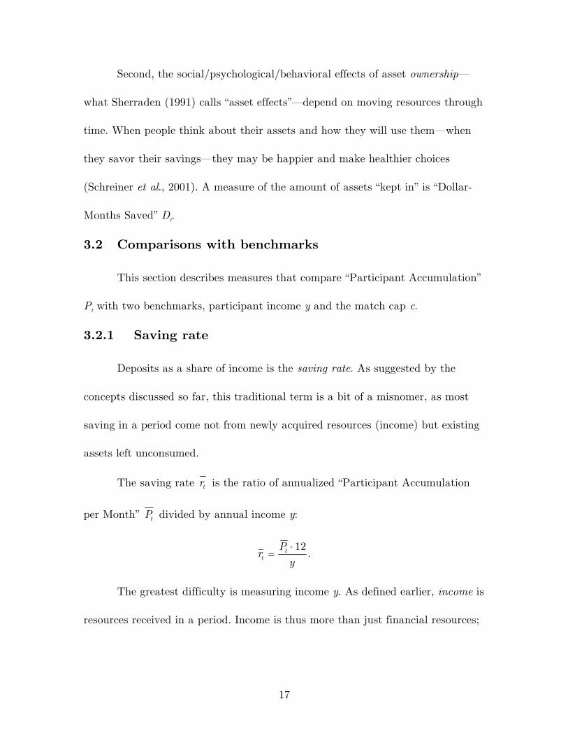
In Figure 1, the “Dollar-Months Saved Ratio” rtD is the area under line A

(Dt·24) divided by the area under line B (c·t·(t+1)). In the figure, the ratio is 0.6.

With no excess deposits, the maximum “Dollar-Months Saved Ratio” rtD is 2 (a

single deposit in the first month equal to (t·c)/12). The minimum of 0 obtains if

there are never any deposits. The ratio is 1 if the pattern of the sizes and timings

of cash flows produces “Dollar-Months Saved” Dt equal to what it would be with

equal, consistent deposits of c/12 each month. (A rate of 1 is possible even if

deposits are not c/12 in each month.)

In the earlier example of two savers, suppose the annual match cap c is

$120. The slow-and-steady saver saved $10 a month and reached the match cap

by year-end. Accordingly, the “Dollar-Months Saved Ratio” rtD is ($780·24) /

($120·12·13) = 1. For the saver who made only one deposit of $120 in December,

rtD is much lower, ($120·24) / ($120·12·13) = 0.154.

3.1.8 Summary

Why bother with so many savings measures? First, the effects of asset use

(such as a down payment on a house) depend on “Total Accumulation” At. In

turn, “Total Accumulation” depends on the match rate and on “Participant

Accumulation” Pt and thus on months of participation t and “Participant

Accumulation per Month” tP . To capture all this requires measuring not only

“putting in” but also “taking out”.

17

Second, the social/psychological/behavioral effects of asset ownership—

what Sherraden (1991) calls “asset effects”—depend on moving resources through

time. When people think about their assets and how they will use them—when

they savor their savings—they may be happier and make healthier choices

(Schreiner et al., 2001). A measure of the amount of assets “kept in” is “Dollar-

Months Saved” Dt.

3.2 Comparisons with benchmarks

This section describes measures that compare “Participant Accumulation”

Pt with two benchmarks, participant income y and the match cap c.

3.2.1 Saving rate

Deposits as a share of income is the saving rate. As suggested by the

concepts discussed so far, this traditional term is a bit of a misnomer, as most

saving in a period come not from newly acquired resources (income) but existing

assets left unconsumed.

The saving rate tr is the ratio of annualized “Participant Accumulation

per Month” tP divided by annual income y:

.12

yP

r tt

⋅=

The greatest difficulty is measuring income y. As defined earlier, income is

resources received in a period. Income is thus more than just financial resources;

18

for example, the main form of income for most people is time to live. This paper,

however, follows convention and counts as income only financial inflows.

Still, some issues remain. Should income include in-cash public assistance?

What about in-kind public assistance? Although public assistance is indeed part

of income, it is very difficult to measure.

Should measures use income before or after taxes? Because the goal is to

measure disposable resources that might be saved, the best measure is probably

after-tax income.

For what time period should income be measured? Because income

fluctuates from month to month and because there are no official records of

monthly income, measurement should use past-year tax returns, if they exist.

3.2.2 Match use

Do participants save all the way up to the match cap? “Participant

Accumulation” Pt divided by the match cap c (pro-rated for months of

participation t) is “Match Use” tX :

.12/)( tc

PX t

t ⋅=

“Match Use” tX shows the pace of saving relative to the pace that would

take advantage of all potential matches. Someone on pace to use exactly all of

their match eligibility has a ratio of 1. Someone behind this pace is below 1, and

someone ahead of this pace is above 1.

19

3.3 Deposit consistency

Savings incentives such as IDAs aim to promote asset accumulation and

healthy saving habits. Although there is little concrete evidence, many people

believe that slow-and-steady wins the race, that is, consistent savers both

become better savers and end up accumulating more. This section presents two

measures of deposit consistency, one that focuses on the presence of monthly

deposits and one that focuses on distribution of the value deposited.

3.3.1 Deposit frequency

The share of months with a deposit is “Deposit Frequency” tf . (Interest

earned is not counted as a deposit; otherwise, all months would have a deposit.)

If the indicator function I(gt) is 1 if “Gross Deposits” gt is positive and 0 if gt is 0,

then “Deposit Frequency” tf is the ratio of the number of months with a deposit

divided by the number of months t:

.)I(

t

gf

t

jj

t

∑== 1

Higher frequencies indicate greater consistency. If a saver makes a deposit

in all months (maximum frequency), then “Deposit Frequency” tf is 1. The

minimum (no deposits at all) is 0.

The strength of “Deposit Frequency” tf is its simplicity. Unfortunately,

this simplicity is also its weakness; for example, the measure is the same whether

20

someone deposits $10 each month for four months or whether they deposit $1,

$19, $15, and then $4. This weakness may be unimportant if, for learning to

save, what matters is not the size of the deposits but their mere presence.

3.3.2 Deposit entropy

A measure of the distribution of the value of deposits through time is

“Deposit Entropy” te . (As noted above, earned interest is not counted as a

“deposit” for the purposes of this measure.) Based on the classic entropy measure

(Golan, Judge, and Miller, 1996), “Deposit Entropy” te is closer to 0 as deposits

are more concentrated (less consistent) through time and is closer to 1 as

deposits are more uniform (more consistent) through time. The formula is:

.

,lnln

∑

∑

=

=

=

⋅⋅⎟⎠⎞

⎜⎝⎛+=

t

kk

j

j

t

jjt

g

gg

ggt

e

1

1

11

j where

The weaknesses of the entropy measure is its newness and its difficult-to-

interpret units. For example, 0.8 is a more-uniform deposit pattern than 0.6, but

the intuitive meaning of the 0.2 difference is not clear.

The strength of the entropy measure is that it summarizes the entire

distribution of deposits. Unlike other summary measures of the uniformity of

distributions (such as variance or coefficient of variation), entropy is bounded

between 0 and 1 and depends only on the distribution’s shape, not its “height”.

21

For example, suppose a saver deposits $10 and $20. The deposit shares

are 0.33310/30 ==1g and 0.66620/30 ==2g . “Deposit Entropy” te is then:

( ) .082.0)637.0(443.1166.0ln66.033.0ln33.02ln

11 =−⋅+=⋅+⋅⋅⎟

⎠⎞

⎜⎝⎛+=te

For comparison, the variance is [(10 – 15)2+(20 – 5)2] / 1 = 50. With a

mean of (10 + 20) / 2 = 15, the coefficient of variation is 50 / 15 = 3.33.

What if deposits were $1 and $2 instead of $10 and $20? “Deposit

Entropy” te is unchanged, as only “height” of the histogram of deposits through

time changes, not its shape. The variance and coefficient of variation, however,

are now 0.5 and 0.33. Unlike these two common summary measures, the entropy

measure is invariant to the scale of units.

22

5. Conclusion

Saving is moving resources through time. Saving has three stages: putting

in, keeping in, and taking out. Each stage matters because saving can break

down in any of the three stages. This paper has proposed various measures of

savings in all three stages and illustrated their use in the context of Individual

Development Accounts.

The basic measure of resources “put in” is “Gross Deposits per Month”.

The measure “Participant Accumulation per Month” recognizes that some

deposits are consumed and that different people save for different lengths of time.

To measure resources “kept in” and “taken out” through time, the appropriate

measures are “Dollar-Months Saved” and the “Dollar-Months Saved Ratio”. The

“Savings Rate” compares “Participant Accumulation” with income, and “Match

Use” compares “Participant Accumulation” with the match cap. Savings

consistency is indicated by “Deposit Frequency” and “Deposit Entropy”.

23

References Beverly, Sondra G.; Moore McBride, Amanda.; and Mark Schreiner. (2003) “A

Framework of Asset-Accumulation Strategies”, Journal of Family and Economic Issues, Vol. 24, No. 2, pp. 143–156.

Bush, George W. (2000) “New Prosperity Initiative”, speech in Cleveland, OH,

April 11. Edwards, Karen; and Lisa Marie Mason. (2003) “State Policy Trends for

Individual Development Accounts in the United States: 1993–2003”, Social Development Issues, Vol. 25, No. 1–2, pp. 118–129.

Golan, Amos; Judge, George; and Douglas Miller. (1996) Maximum Entropy

Econometrics: Robust Estimation with Limited Data, New York: Wiley, ISBN 0-471-95311-3.

HM Treasury. (2003) “Detailed Proposals for the Child Trust Fund”,

http://www.hm-treasury.gov.uk/media/C7914/child_trust_fund_proposals_284.pdf.

Johnson, Susan; and Thalia Kidder. (1999) “Globalization and Gender—

Dilemmas for Microfinance Organizations”, Small Enterprise Development, Vol. 10, No. 3, pp. 4–15.

Kempson, Elaine; McKay, Stephen; and Sharon Collard. (2003) “Evaluation of

the CFLI and Saving Gateway Pilot Projects”, Personal Finance Research Centre, University of Bristol, http://www.ggy.bris.ac.uk/research/ pfrc/publications/SG_report_Oct03.pdf.

Kessler, Glenn. (2000) “Gore to Detail Retirement Savings Plan”, Washington

Post, June 19, p. A01. Poterba, James M.; Venti, Stephen F.; and David A Wise. (1995) “Lump-sum

Distributions from Retirement Saving Plans: Receipt and Utilization”, National Bureau of Economic Research Paper 5298, papers.nber.org/papers/w5298.pdf.

Samwick, Andrew A.; and Jonathan Skinner. (1997) “Abandoning the Nest Egg?

401(k) Plans and Inadequate Pension Saving”, in Sylvester J. Schieber and John Shoven (eds) The Economics of U.S. Retirement Policy: Current Status and Future Directions, Cambridge, MA: MIT Press.

24

Schreiner, Mark; Sherraden, Michael; Clancy, Margaret; Johnson, Lissa; Curley,

Jami; Grinstein-Weiss, Michal; Zhan, Min; and Sondra Beverly. (2001) Savings and Asset Accumulation in Individual Development Accounts, Center for Social Development, Washington University in St. Louis, gwbweb.wustl.edu/users/csd/.

Schultz, Theodore W. (1979) “Nobel Lecture: The Economics of Being Poor”,

Journal of Political Economy, Vol. 88, No. 4, pp. 639-51. Sherraden, Michael. (1991) Assets and the Poor: A New American Welfare

Policy, Armonk, NY: M.E. Sharpe, ISBN 0-87332-618-0. _____. (1988) “Rethinking Social Welfare: Toward Assets”, Social Policy, Vol. 18,

No. 3, pp. 37–43. Vonderlack, Rebecca M.; and Mark Schreiner. (2002) “Women, Microfinance,

and Savings: Lessons and Proposals”, Development in Practice, Vol. 12, No. 5, pp. 602–612.

Wayne, Leslie. (1999) “U.S.A. Accounts Are New Volley in Retirement Savings

Debate”, New York Times, Jan. 24, p. 4.

25

Figure 1: The “Dollar-Months Saved Ratio”

0 t

Months

Bal

ance

Line B (deposit c/12 each month)

Line A (deposit (0.6*c)/12 each month)