1

Measuring Risk and Time Preferences and Their Connections with Behavior

Julian Jamison, Dean Karlan, and Jonathan Zinman*

August 19, 2012

CITES AND SUPPORTING MATERIALS INCOMPLETE, BUT READY FOR COMMENTS

*julison@gmail.com, Federal Reserve Bank of Boston, IPA; dean.karlan@yale.edu, Yale University, IPA, J-PAL, and NBER; jzinman@dartmouth.edu, Dartmouth College, IPA, J-PAL, and NBER. Thanks to Lynn Conell-Price, Hannah Trachtman, and Gordon Vermeer for outstanding research assistance, and to the Russell Sage Foundation for funding.

2

I. Introduction

The economics profession builds models based on individual preferences. Estimating values for preference parameters is important for both testing and applying our models. For testing models, preference parameter estimates allow us to assess the predictions models make about relationships between preferences and choices or outcomes. For applying models, preference parameter estimates are inputs for measuring welfare and conducting policy analysis. We examine methods for measuring individual preferences directly not because observing choices is bad, but specifically because we want to understand better the link between preferences and choices. A “revealed preference” approach alone yields inferences that conflate other issues. For example, data on insurance choices may be used to estimate risk preferences, but time preferences, perceptions and unobserved individual heterogeneity in true underlying risk also drive insurance purchase decisions [cite/fn on work that does this by imposing assumptions?]. Similarly, is our tardy production of this paper due to our stable preferences for leisure versus work; to aspects of our choice set that may be mistakenly confounded with our preferences; to procrastination deriving from time-inconsistent preferences (and the absence of a commitment device with a higher cost of failure than the shame of receiving polite but increasingly firm warning emails from the editors); or to a planning problem in which we systematically underestimate the time for the remaining tasks? By eliciting measures of preferences directly, and linking such measures to behavior, we can better validate the underlying model to explain choices. We consider evidence on the direct elicitation of three broad classes of individual preferences. Our coverage of risk preferences includes risk aversion as classically defined, and also ambiguity aversion and loss aversion. Our coverage of time preferences includes the classic issue of how to disentangle preference from other determinants of discount rates, and also time-inconsistency and other sources of costly self-control. Our coverage of process preferences (includes regret and transaction utility) is much shorter, reflecting the lack of similar work on measurement. We thus focus more on identifying key gaps in our knowledge for further research. We do not cover atemporal preferences over different goods in a consumption bundle, or social preferences (see [cites] for reviews). Nor do we cover meta-awareness of one’s (changing) preferences—e.g., projection bias, sophistication/naivete about self-control problems-- about which there has been less work on direct elicitation. For both risk and time preferences we address four types of questions: methods, predictive power of actual behavior, heterogeneity across people, and within-subject stability. On methods, we describe the various commonly used elicitations, and examine how different elicitation and estimation methods affect parameter estimates. Key examples include the roles of monetary incentives versus hypothetical questions; quantitative versus qualitative questions; potential confounds researchers should consider when choosing an elicitation method (e.g., how numeracy may influence lottery choices, and disentangling risk perception from risk preference); and some “quick-and-dirty” methods for researchers facing budget and/or time constraints in the lab or the field.

3

Second, we examine how measures predict actual behavior. The primary challenge with posing this question is simple: one needs clean measurement on both sides of the correlation, free of alternative explanations that happen to also correlate with each other. Let’s start with a simple example of the problem. Suppose we want to validate a model of time preferences and investment in new agricultural technology. The policy idea is simple: farmers may not invest in highly profitable investments if they are impatient and thus prefer current consumption to considerably more future consumption. So researchers conduct simple time preference elicitation questions (would you prefer money now or more money later?), and observe if they invest in a higher yield agricultural technology. The researcher finds they are correlated. What can be concluded? Perhaps also the higher yield agricultural technology requires trusting the agricultural extension agent. And so does accepting more money later rather than money immediately. If this were the case, trust, but not necessarily time preferences, would be the underlying mechanism at work. These problems with interpreting correlations between preferences and behavior are likely difficult to overcome perfectly, but must be whittled down as much as possible in order to advance our knowledge on the validity of such measures. Timing is helpful, but not dispositive. If measurement occurs, and then much later the behavior is observed, this may help eliminate reverse causality (although naturally does not remove a myriad of other unobservable correlates). This was the approach taken, e.g., in Karlan (2005) in which trustworthy behavior in a trust game was found to predict repayment of loans a year later, and in Ashraf, Karlan and Yin (2006) in which inconsistent responses to time preference questions predicted later adoption of a commitment savings product. To make this link from preferences to behavior, however, requires a strong methodological emphasis on the details on elicitation methods, and also strong contextual understanding of the decisions people face in the real world, that one is trying to model. Third, we ask how heterogeneous are estimates cross-subjects, and what are the determinants of heterogeneity? This speaks to, among other things, the descriptive power of representative agent models, and to our (limited) ability to “explain”, or at least fit, preferences with observable characteristics. Fourth, we examine how (un)stable parameter estimates are within-subject, across time. This question speaks to meta-questions about what preferences capture (something inviolable and deep, versus something more malleable and highly context-specific). In this context, we also discuss interventions designed to change preferences. We know of only a few cases of the latter, primarily in the context of impatience and self-control. Our approach here errs on the side of breadth, not depth. We hope that each section highlights the challenges involved in the direct elicitation of that set of preferences and their impacts on behavior, in ways that encourage further progress in the development of elicitation methods. We try to be comprehensive about identifying the issues that researchers need to confront, rather than being comprehensive about resolving said issues. Part of this is due to necessity: for most types of preferences, we could find little warranted consensus on best-practice methods. Part of this is due to taste, in that we believe many of the most important research questions here revolve

4

around how to disentangle specific types of preferences from other preferences, from other cognitive inputs into decision making (like expectations, price perceptions, and memory), and from elements of choice sets (like liquidity constraints, and returns to capital).

II. Uncertainty

A. OverviewofTheoriesandConcepts

Preferences with regard to uncertainty are generally regarded as one of the most fundamental or “primitive” aspects of someone’s utility function. As such, inferences about the nature of these preferences are of vital importance to virtually every discipline and subfield in the social sciences. The experimental study of preferences over risk/uncertainty has breadth and depth commensurate with its importance; a thorough study would be at least book-length (as evidenced by [Cox and Harrison 2008]). As such we provide a primer rather than a manual, and refer the interested reader to Cox and Harrison [2008], and other references below, for further details. We start with the important distinction between attitudes towards and preferences over uncertainty. Attitudes, as typically defined, are a reduced-form combination of both preferences and perceptions about risk likelihood (and/or the cost/benefit of different states of the world conditional on their realization). E.g., someone may exhibit risk averse behavior because of their underlying preferences, conditional on (possibly distorted) expectations, and/or they may exhibit risk averse behavior because of their expectations. So a question that asks: “Do you tend to take risks in choosing when to harvest your crops?” may pick up elements of risk preference (I don’t take the risky action because I have very concave utility and am not willing to expose myself to variance in income), and/or of risk perception (I don’t take the risky action because I perceive bad states of the world, e.g. a heavy rainfall at harvest time, to have a high probability). We avoid the notion of strategic uncertainty, which is due to another agent’s behavior rather than states of nature.1 A brief overview of different theories helps set the stage. Expected utility theory (EUT) reduces preferences over uncertainty to “risk”. Agents face known distributions of probabilities of all states of the world, and perceive these probabilities accurately. Risk preferences can then be categorized in one of three ways: risk aversion (preferring a certain payoff lower than the expected value of a gamble to the gamble itself), risk-seeking (preferring the gamble to a certain payoff equal to the expected value) or risk-neutrality (linear utility). In order to better facilitate this categorization, Arrow [(1965) and Pratt [(1964) formalized two local measures of risk-aversion, relative risk aversion (RRA) and absolute risk aversion (ARA,) 2 both of which are positive for risk aversion and negative for risk seeking. Studying risk preference under EUT frequently involves estimating these parameters. It can also involve sketching the utility function more globally, since the study of risk preferences under EUT is equivalent to studying the function’s curvature. However, EUT implies approximate risk neutrality over anything but large

1 For instance, by observing the relative frequency of choices of the risk-dominant action in the stag-hunt game, one could measure the strategic risk-aversion of an individual. 2 RRA is defined as – and ARA is defined as –

′′

′ .

5

stakes [Rabin 2000], which is a problem for elicitation methods that use small stake questions to calibrate EUT models.3 Other theories posit more complicated structures of preferences over uncertainty. Some complications are due to allowing for added richness or bias in risk perception (e.g., lack of clear or accurate expectations), as in cumulative prospect theory [Tversky and Kahneman 1992], salience theory [Bordalo et al 2012] or ambiguity aversion. Other complications are due to nonlinearities or other discreteness in preferences; e.g., loss aversion in prospect theory, preference for certainty [see, e.g., Andreoni and Sprenger _UCE_ 2012] or rank-dependent utility [Quiggin 1982]; see also Fudenberg and Levine [2012]. Hey [1997] and Starmer [2000] provide a more complete set and description of alternatives to EUT. As with EUT, researchers can use data elicited from choice tasks, in combination with various econometric approaches, to estimate model parameters and/or utility functions under various (often testable) assumptions.

B. Methods

1. Methods:ElicitationandEstimation4

There are several general methods to elicit preferences or attitudes over uncertainty. We describe each in brief, along with a summary of key limitations or concerns. Our Appendix contains a concrete example, for each elicitation method, of a choice task or survey question used in that method. We focus on direct elicitation and do not cover papers that infer preferences from field data; see e.g., [Einav et al] for a recent paper using this approach. The Multiple List Price (MPL) method [Miller et al 1969] offers choices between two or more uncertain prospects with fixed payoff amounts and varying probabilities. In the widely-used Holt and Laury [2002] version of MPL, subjects face a single list (visible all at once) of binary decisions between two gambles. The payoffs remain the same in each decision but the probabilities vary, meaning that any respondent with consistent risk preferences should have a “switch” point between preferring gamble A or gamble B (we discuss models that allow for a “trembling hand” or other types of choice-inconsistency in Section []). Tanaka et al [2010] offer a new variant of MPL that elicits utility curvature, curvature of the probability weighting, and the degree of loss aversion (and of time preference) under various assumptions. MPLs have been criticized for assuming linear utility (as discussed in Section III, discount rate estimates from MPLs are biased upward if utility is concave), and for providing interval rather than point identification of preference parameters. The Ordered Lottery Selection method [Binswanger 1980; 1981; Barr 2003] offers choices between two or more uncertain prospects with fixed probabilities and varying payoff amounts. As Harrison and Rutström [2008] discuss, it has been conventional to use 0.5 as the fixed probability, and to offer a certain option along with (several) gambles. These conventions create difficulties for estimating non-EUT models but are not intrinsic features of the design: one could

3 For example: say a person turns down a gamble where he has equal probability of losing $100 or gaining $110. If the only explanation is curved utility, this implies that he will spurn any gambles with equal probability of losing $1000 or gaining any positive amount, no matter how large it is.. 4 Here we borrow especially heavily from the taxonomies and discussions in Harrison et al [2007] and Harrison and Rustrom [2008].

6

use a range of probabilities to allow for estimates of probability weighting, and one could eliminate the certain option, and/or vary how the different gambles are arrayed, to test or control for framing/reference point effects [Engle-Warnick et al 2006] A few studies use methods that provide a continuum of choices (in contrast to the discrete choices posed by MPL and OLS), using linear budget constraints. (We discuss the convex time budget method later in this sub-section, and again briefly in the section on time preferences.) Andreoni and Harbaugh [2010] provide choices between gambles with probability of winning an amount x with probability p<1. Choices trade off probability for prize. Choi et al [2011] provide choices between two differently priced assets that each have the same gross payoff per unit, and a 50-50 chance of paying out or paying nothing. So a (locally) risk neutral subject should allocate all experimental income to the cheapest asset, and the share of income allocated to the cheapest asset is a measure of risk tolerance. The certainty equivalent (CE) method adapts the Becker, DeGroot, and Marschack [1964] (BDM) procedure by endowing a subject with a one or more lotteries and then asking for her selling price for each lottery [Harrison 1986].5 The subject is told (and, in some implementations, shown) that a buying price will be picked at random, and that if the buy price exceeds (does not exceed) the subject’s stated sell price, the lottery will be sold (not sold) and the subject will receive her sell price (play the lottery); i.e., she will receive (not receive) her CE. Other CE methods use a list of choices, in the spirit of MPL, rather than direct elicitation; e.g., in Tversky and Kahneman [1992] the respondent must choose between a gamble (which stays constant throughout the trial) and a series of sure payoffs.6 The use of this choice-based method is motivated in part by work showing that it produces more internally-consistent results than direct elicitation of CEs [Bostic et al 1990]. Plott and Zeiler [2005] and Harrison and Rutström [2008] raise some concerns with standard implementations of the CE method: subjects may misunderstand the payoff structure of BDM elicitation and engage in misguided strategic misstatement of their CE’s, and within-session (co-mingled) income and learning effects can confound inferences about preference parameters. Both papers offer tweaks to instructions and treatments that are designed to mitigate these concerns. The Barsky et al [1997] lifetime income gamble (LIG) battery is a (relatively small) set of hypothetical choices between a job that, with 50-50 probability, either doubles lifetime income or cuts it by a (varying) fraction, and a job that pays a certain lifetime income. So the general elicitation method is a hybrid CE/MPL. LIG’s innovations are the contextual focus on lifetime income (which, for many theoretical and practical applications is more interesting/important than the siloed choices often used to elicit risk preferences), and tractability: LIG is relatively quick and easy to administer. LIG has been adopted and adapted by nationally representative household surveys across the world. Its main limitations are its coarseness (although Kimball et al [2008, 2009] provide an econometric method for imputing quantitative estimates of the

5 The probability equivalent (PE) method, where a subject is asked to supply a probability at which she would play a lottery with two specified payoffs instead of taking a certain payoff, seems to us justifiably less popular (in economics at least) these days than the other methods discussed here, given concerns about probability weighting and numeracy (see Section []). 6 Specifically, the range of sure payoffs is then adjusted to include values spaced closer together and near the “switching point” from the first series, in order to refine the certainty-equivalent estimate.

7

coefficient of relative risk tolerance from LIG responses under CRRA, EUT, and other functional form assumptions), its reliance on hypothetical stakes (see Section [] below), and a potential confound with discount rates (depending on what respondents assume about the exact meaning of “double”; e.g., timing of income flows). The trade-off (TO) method [Wakker and Deneffe 1996] is a variant of CE where subjects choose between pairs of lotteries. TO permits inference about risk parameters without any assumptions about whether the subject weighs or misperceives probabilities (in contrast, standard CE methods assume no probability weighting, which is paradoxical because prospect theory, the motivating theory behind many applications of CE methods, posits probability weighting). Abdellaoui et al [2007] extend the TO method to facilitate estimation of a loss aversion parameter. However, there are two thorny problems with the TO method. The first and arguably most serious is a lack of incentive compatibility that, as far as we can tell, is intrinsic to the method: subjects have an incentive to overstate their CE. The second, somewhat more tractable problem is that, since responses to any choice after the first one depend on previous responses in the TO method, there is potential for error propagation [Abdellaoui 2000]. The uncertainty equivalent (UCE) method identifies indifference between a gamble, and the probability mixture over the gamble’s best outcome and zero [Andreoni and Sprenger 2012; Callen et al 2012]. To take Andreoni and Sprenger’s example, consider a gamble G1 that pays $10 probability p or $30 with probability 1-p. Now consider a gamble G2 that pays $30 with probability q, and $0 with probability 1-q. The UCE is the probability q that makes the subject indifferent between G1 and G2. Andreoni and Sprenger [2012] use UCEs to test the independence axiom (see Section [] below)—independence implies a linear relationship between p and q-- and the relative descriptive power of EUT, CPT, and u-v models away from and near certainty (i.e., over choices involving only risky options, and over choices involving a safe option). [critiques of this method?] Fehr and Goette [2007] provide a quick method for estimating loss aversion from two choices. One choice is between zero with certainty versus “Lottery A”: a 50% chance of winning 8 and a 50% chance of losing 5. The other choice is between zero with certainty versus playing six independent repetitions of Lottery A. Identifying loss aversion per se with these tasks requires two potentially problematic assumptions: linear utility over the stakes under consideration, and no probability weighting. Several surveys have asked purely qualitative questions that are designed to elicit risk attitudes. Noteworthy among these are those included in several European household surveys, which ask “Do you consider yourself a risk-taker [overall, or in domain X]?”, and the Survey of Consumer Finances’ question about the “amount of financial risk that you… are willing to take…” (with response options ranging from “Take substantial financial risks expecting to earn substantial returns” to “Not willing to take any financial risks”).7 The merits of this sort of approach are the easy and low-cost implementation, and the strong, positive correlations between measures of risk

7 See also Meertens and Lion’s (2008) Risk Propensity Scale, which asks respondents to agree or disagree with seven “unrelated” statements about their risk propensity; e.g., “I really dislike not knowing what is going to happen” (which economists would think of as pertaining to ambiguity more than risk; see following section), and “I do not take risks with my health”.

8

tolerance inferred from responses and behavior/outcomes like wealth or risky asset holdings [Dohmen et al 2011; Stango and Zinman 2009]. It may be the case that short qualitative questions are more easily understood by respondents, and/or completed with less effort, and thereby deliver more precise and/or more informative estimates. But what exactly do these qualitative responses identify? Clearly they do not readily yield point identification of any preference parameter (although in principle they could be useful for ordinal ranking). Indeed, the evidence on whether and how responses to qualitative questions are correlated with parameter estimates obtained from choice task methods is limited, and mixed (see Dohmen et al (2011) vs. Lonnqvist et al [2011]). The data thus far is also reduced-form in the additional sense that the survey responses presumably reveal something about risk perception (e.g., the likelihoods of various states) as well as risk preference (how I value, in utility terms, the realizations of various states). In principle, one could elicit perceptions—indeed, there is a large literature on eliciting risk perceptions—along with attitudes, and then use the information on perceptions to help back out (ordinal) preferences. We are not aware of any papers taking this exact approach with qualitative questions, but it seems like a potentially profitable one, and has been employed with quantitative elicitations by Andersen et al [2010]. Most of the work comparing different elicitation methods uses within-subject designs, and not all of these studies (fully) control for order effects. This is a real concern given the possibility of learning, fatigue, wealth effects, and other sources of within-subject preference “instability” (Section []). So one should be circumspect when drawing inferences from these studies, and it seems to us that there would be value in new studies that use between-subject designs (as in Harrison et al’s [2007] analysis of prize type and lottery framing), and/or within-subject designs that carefully control for order effects. More studies using non-EUT specifications would also help better link this line of inquiry to the rest of the literatures. The general consensus seems to be that inferences depend significantly, and often dramatically, on elicitation method (Anderson and Mellor [2009]; Dave et al [2010]; Deck et al [2008]; Hey et al [2009]; Reynaud and Couture [2010]; Andreoni and Sprenger [2012 Uncert Equiv]; Andreoni and Sprenger [2012 estimation]).8 This can hold even within classes of the “general elicitation methods” described above, as in Isaac and James’ [2000] and Berg et al’s [2005] comparisons of different CE methods. Harrison and Rutström [2008] is an exception to the consensus that elicitation method matters a lot: they obtain similar estimates for CRRA from the MPL of Holt-Laury [2002], the random lottery pairs of Hey and Orme [1994], and the ordered lottery selection of Binswanger [1980; 1981]. Several studies conclude that some methods produce less noise (or, more precisely, greater within-subject, within-task consistency) than others. Hey et al [2009] find that MPL is more precise than CE methods. Anderson and Mellor [2009] find that correlations between Holt-Laury MPL and hypothetical gambles with time horizons are stronger among subjects who make consistent choices (a la [Choi et al 2011]). Dave et al [2010] find that a simplified Binswanger

8 Hershey and Schoemaker [1985] find substantial differences across CE vs. PE tasks for hypothethical gambles, and review the early literature on “response mode biases” and other sources of differences across elicitation methods using hypotheticals.

9

task (a la Eckel and Grossman [2002, 2008]) produces more informative CRRA estimates, among low-numeracy subjects, than a more complicated MPL task. Harrison and Rutström [2008] cover the “what to do with the data” question in detail, for both EUT and non-EUT models, so we focus on some recent developments. One recent development is the joint estimation (and elicitation) of risk and time preferences, which has been motivated primarily by the concern that moving payoffs to the future (in order to elicit time preferences) introduces risk. Another, less-scrutinized source of motivation is that evaluating risk preferences over time horizons is often of interest (e.g., with respect to lifetime income), and this introduces potential confounds with time preference. There are two main approaches for jointly eliciting risk and time preferences (see also Section [] below). Andersen et al [2008] employ separate multiple price lists, one for riskless choices over time, or one for risky choices paid out immediately (see also Andersen et al [2011]). Laury et al. (2012 JRU) are able to approximately replicate these discounting results by using a novel “risk-free” intertemporal-choice task. Andreoni and Sprenger use convex time budgets (CTBs), where subjects allocate a convex budget of experimental tokens to sooner and later payments. Variation in sooner and later times, slopes of the budgets, and relative risk are used to identify parameters and test theories. Andreoni and Sprenger [2012 Estimation] use riskless choice over time to estimate utility function curvature, which is equivalent to risk aversion under expected utility. Andreoni and Sprenger [2012 RiskTime] uses CTBs with risky choices to test the common ratio prediction of discounted expected utility theory. For discussions of the pros and cons of each method, see the papers cited in this paragraph. Another recent development is the application of mixture models for classifying individuals as EUT or non-EUT (e.g., CPT, or Rank-Dependent Expected Utility) types [Harrison and Rutström 2009 EE; Bruhin et al ECMA 2010; Conte et al 2011 Journal of Econometrics]. See also Choi et al [2007 AER]. These approaches seem fruitful in light of the mounting evidence of substantial preference heterogeneity across individuals (see Section []). The use of dynamic survey design (relying on real-time estimation of which subsequent question/task, from a pre-set menu, will elicit the most precise information on a subject’s preferences) also seems promising. Toubia et al [2011] adapt a dynamic method used in conjoint analysis to the estimation of CPT parameters (and to estimation of a quasi-hyperbolic time discounting model as well).

2. Methods:RealStakesversusHypothetical

The question of whether/when/why a researcher should use real stakes, rather than hypothetical questions, to elicit risk preferences has been ably addressed by, among others, Camerer and Hogarth [1999], and Harrison [2007].9 Focusing on comparisons of the same method with versus without real stakes, we have not been able to find much work that post-dates Harrison [2007 book chapter]. One exception is Laury and Holt [2008], which finds that evidence of asymmetry in risk preferences over gains versus losses is larger with hypothetical than real stakes, and further attenuated as the stakes get larger. Another recent contribution is von Gaudecker [AER 9 Note we refer to this as real stakes versus hypothetical, not “incentivized” versus “not incentivized”, out of respect for the great American philosopher Calvin, who said to Hobbes, “verbing weirds language.”

10

2011] which finds that stakes (or lack thereof) change parameter estimates for risk aversion and loss aversion. In all, it seems that there is a consensus that stakes matter: estimates of various risk preference moments are different under different-sized stakes. It bears noting, however, that merely finding that the two methods yield different answers does not mean that using stakes is necessarily the better one method (particularly given the cost, i.e, if merely to reduce measurement error, there is a genuine tradeoff between sample size and measurement error). More direct comparisons of how real stakes versus hypothetical elicitations correlate with (real-world) behavior would help (see section below on predicting real behavior). There are some compelling reasons for relying on hypothetical questions. For example, stakes may exceed research budgets, or gambles may be over long horizons, or complications may exist with respect to corruption and cash management in handling the cash in the field. These reasons may come to include an inherent tension between an assumption needed for standard 1-in-K payment mechanisms to make sense (the independence axiom), and the assumption (and accompanying evidence) that that same assumption is systematically violated when subjects make multiple choices (see our discussion of Harrison and Swarthout [2012], and related work, below). Ethical considerations involved in imposing losses on subjects does not, in and of itself, strike us as a compelling reason to rely on hypotheticals. One can provide subjects with an endowment and design gambles such that, even under the experiment’s worst-case scenario, the subject does not lose more than her experimental endowment (although this does require some assumptions regarding how the show-up money is accounted for, mentally, by the participant). So if the default is to use real stakes, the next question is: how? Important work is emerging on how different types of incentive mechanisms affect choices, and the inferences we can make from them. Cox et al [2011] and Harrison and Swarthout [2012] find that estimates of rank-dependent utility risk preferences differ depending on the payment protocol (see also [Laury “Pay One or Pay All” 2006]): 1-1, where the subject makes only one choice and is paid based on that choice [Conlisk 1989], versus the standard “1-in-K” payment protocol [Starmer and Sugden 1991]. This finding suggests, perhaps not surprisingly (given evidence on probability weighting), that the oft-invoked convenient assumption of an “isolation effect” (subjects view each choice as independent of the others) is violated. Violation of this independence axiom (IA) makes it challenging to construct incentivized tasks that elicit valid, high-powered inferences on non-EUT theories where the IA does not hold. Cox et al [2011] test two new payment mechanisms that should, in theory, be incentive-compatible under special cases: Yaari’s [1987] particular form of rank-dependent utility, and Schmidt and Zank’s [2009] linear cumulative prospect theory. Cox et al [2011] also test two other payment mechanisms and find that they induce wealth effects, portfolio effects, and adding-up effects that can confound inferences. Andreoni and Harbaugh [2010] and Andreoni and Sprenger [2011 UCE] test the independence axiom using two different methods, and find that it holds only away from certainty (see also Callen et al [2012]).

11

3. Methods:OtherDesignConsiderations

Apart from the issues with stakes discussed directly above, and some rather obvious considerations (allowing for losses if you want to study loss aversion, allowing for certain options if you want to study direct risk aversion), there are several other important considerations when designing an elicitation method. For some lines of inquiry using multiple-decision tasks it may also be important to consider how visible the subject’s prior decisions are, in order to disentangle effects of memory, salience, and/or framing on choices from effects of preferences One fundamental consideration, embedded in many non-EUT theories, is a distinction between preferences and perceptions. If people do not have accurate perceptions of likelihoods—if they “subjectively weight” probabilities—then choices can reflect distorted perceptions (which may be amenable to correction) rather than preferences (which are inviolate over some timeframe). There are various methods for eliciting and/or estimating subjective probabilities or “decision weights”; see e.g., Andersen et al [2010], Blais et al [2002], [Bruhin et al 2010], [Bruine de Bruin et al 2007], [Toubia et al 2011]. Another consideration is framing: how a task is presented or described (e.g., as an “investment” or a “gamble”) can affect choices, independent of its economic content as defined by EUT [Peters et al 2006; Deck et al 2008]. Depending on the line of inquiry, framing effects may be second-order and easily correctable (e.g., Harrison and Rutström [2008, section 1.1]), while in other instances framing may be more central. For example, work on non-EUT theories where reference points are critical (prospect theory, salience theory) must think carefully about how subjects bring reference points into, and/or form them under, the elicitation task (see, e.g., Ericson and Fuster [2010]). Work on rank-dependent utility models must pay particularly close attention to whether a given outcome is framed as a gain or a loss [e.g., Sitkin and Weingart (1995)]. Frames can have unexpected effects, however. Harrison et al [2007 ECMA] find that a frame designed to make people less risk averse (by providing smaller increments in the probability for risk loving choices than for risk averse choices) actually made people more risk averse. Beauchamp et al [2012] find that a frame designed to make people more risk-neutral (by providing the expected values of risky prospects) had no effect. A related consideration is that loss aversion creates incentives for people to use “creative mental accounting” [see Thaler 2004 “Mental Accounting Matters”]. E.g., accounting for a loss of 10 and a gain of 20 as a net gain of 10 may deliver greater utility than “booking” the two transactions separately. (We are distinguishing between underlying preferences and decision making approaches—heuristics, etc.—operationalized in service of those preferences.) Understanding how and when subjects (strategically) bracket decisions and outcomes, on the narrow vs global continuum, may be critical for obtaining an accurate picture of preferences per se. Another emerging consideration is whether to jointly elicit multiple aspects of preferences (e.g., risk and time, risk and ambiguity). Joint elicitation can save time (Section [], and may be needed to produce unbiased estimates of preferences over uncertainty (Section []).

12

Another consideration is how to deal with within-subject internal inconsistency that is not explicable by simple/literal versions of any of the leading models of preferences over uncertainty. Some approaches provide econometric corrections or allowances for response error (see, e.g., Hey and Orme [1994]; Harrison and Rutström [2008]; Toubia et al [2011]). Other approaches take internal inconsistency as a behavioral object of interest [von Gaudecker et al AER 2011; Choi et al Who is More Rational; Parker and Fischoff 2005], and/or as a cognitive factor that may interact with risk preferences [Jacobson and Petrie 2009]. A closely related consideration, long a focus of experimenters, is whether subjects understand the task/question. Simpler tasks, even if they map imperfectly to theory, may produce better estimates of a concept—more precise, and/or less confounded with omitted variables. Similarly, controlling for likely omitted variables (such as numeracy or cognitive ability – see e.g. Frederick’s [2005] “cognitive reflection task”) may improve estimates but of course risk problems if the underlying preference also shifts the now-included omitted variable (e.g., if being impatient leads one to invest less in education, and thus core worse on cognitive tests, then including a control for cognition would bias the true effect of impatience on the outcome of interest). Background risk (a risk that is correlated with a risk used to elicit preferences) is another important consideration. Harrison et al [ECMA 2007] find that background risk can affect inferences, and they discuss implications for field and lab design, including controlling for and/or experimentally manipulating background risk. Harrison et al [ECMA 2007] also study the closely related question of what good to gamble over (money vs. rare coins, in their case).

C. PredictivePowerofMeasuresonRealBehavior

Evidence on whether and how elicited estimates of preferences over uncertainty correlate with real-world behavior/outcomes is limited, mixed, and inconclusive, in large part due to the potential for massive omitted variables problems stemming from the (often unobserved) heterogeneity in preferences and behavior described in Sections [] and []. Cardenas and Carpenter [2010] nicely summarize the mixed state of prior evidence (focusing on studies set in developing countries), and conduct their own analysis by linking rich survey data from subjects in six Latin American cities on economic well-being (including access to credit) with incentivized tasks to elicit preferences over risk, ambiguity, and losses. They find no robust conditional correlations between risk preferences (estimated using a short Binswanger-like task where subjects were shown a ring of six binary lotteries and asked to pick one to play) and economic status, but do find some evidence that ambiguity aversion is correlated with poverty and that loss aversion is correlated with wealth. Tanaka et al [2010] find that MPL estimates of risk aversion and loss aversion are not conditionally correlated with household income (Table 4). Choi et al [2011] find no significant conditional correlation (p-value 0.12) between risk tolerance (estimated using one of the linear budget constraint methods decribed in Section []) and wealth in a representative sample of Dutch households, although the point estimate implies an economically large negative association. Of course, one can debate whether or not wealth is a behavior in the sense that smoking or stock

13

market participation (see below) unequivocally are. We could as easily have included these studies in the follow subsection on individual heterogeneity and correlates. Johnson et al [2010] find that risk aversion and loss aversion (estimated using the Toubia et al [2011] method) are uncorrelated with being “under water” on a mortgage. In the same vein, but turning more specifically to individual choice behavior, risk tolerance inferred from the lifetime-income gamble questions are (fairly) strongly conditionally correlated with share of financial wealth in stocks [Barsky et al 1997; Kimball et al 2008], stock market participation [Hong et al 2004 Table III] and other risky behaviors like smoking, drinking, and not having insurance [Barsky et al 1997], as measured in U.S. surveys. Anderson and Mellor [2008] find that risk aversion (estimated using Holt-Laury MPL) is negatively and significantly conditionally correlated with several unhealthy behaviors and outcomes in a sample of Virginia adults. Lusk and Coble [2005] find that risk aversion (estimated using Holt-Laury MPL) is negatively correlated with eating genetically-modified food among student subjects, conditional on risk perception and some demographics. Guiso and Paiella [2008] find that risk aversion (as inferred from a CE hypothetical on a risky security) is strongly unconditionally correlated with some (risky) behaviors but not others in an Italian survey. Finally, Fehr and Goette [2007] find that only loss-averse individuals (as measured using their method described above) exhibit less effort when wages increase. Qualitative measures of risk attitudes are strongly conditionally correlated with various outcomes in intuitive ways, as discussed in Section [] above.

D. Correlates(heterogeneityacrosssubjects)

Harrison and Rutström [2008, p. 130] conclude that: “At a substantive level, the most important conclusion is that the average subject is moderately risk averse, but there is evidence of considerable individual heterogeneity in risk attitudes in the laboratory.” The first conclusion is critical in that it casts doubt on the usefulness of EUT as a (leading) workhorse model [Rabin 2000]. The second conclusion effectively lays out a challenge: our workhorse model(s) of decision making under risk/uncertainty must be able to accommodate substantial heterogeneity in preferences (or at least in behavior). Nothing has emerged, insofar as we have seen, to change or modify those conclusions based on method, mode, setting, or subject population. To take just a few recent examples from studies based on large representative samples,10 Von Gaudecker et al [AER 2011] find substantial dispersion in risk aversion and loss aversion inferred from incentivized MPL choices offered to a nationally representative sample of Dutch survey-takers (see also Choi et al [2011]). Kimball et al [2008; 2009] find substantial heterogeneity in CRRA, among a nationally representative sample of U.S. survey-takers, estimated from the Barsky et al [1997] hypothetical gambles over lifetime income. Dohmen et al [JEEA 2011] find substantial heterogeneity in responses to qualitative questions about risk attitudes (Section 2.3.b) in a nationally representative sample of German survey-takers. Cardenas and Carpenter [2010] find substantial heterogeneity in risk [and ambiguity?] preferences, inferred from incentivized Binswanger-like tasks, among large representative samples from six Latin American cities. 10 Other studies finding substantial heterogeneity among non-student samples include Andersen et al [JEBO 2010], Attanasio et al [forthcoming AEJ: Applied], Burks et al [2007, Figure 10], and Tanaka et al [2010 AER].

14

A key issue is whether convenience samples (usually university students) have preferences that are representative of the broader population(s) of interest. Andersen et al [JEBO 2010] examine this question in Denmark using MPL and obtain similar estimates of the CRRA on average, with substantially more heterogeneity in the “field” (non-student-specific) sample.11 It is worth noting that barriers to sampling from (more) representative and other non-student samples have never been lower, and seem to be falling, with development of internet survey (panels), Time-Sharing Experiments for the Social Sciences, and other channels (see the Conclusion for further discussion). Much has been made about heterogeneity in risk preferences by gender, race, parental background, height, etc. [in addition to the papers cited in this section, see also Donkers et al [2001]; Eckel and Grossman [2008]; Croson and Gneezy [2009]], but overall, there is evidence that far more cross-subject heterogeneity is due to unobserved than observed characteristics (e.g., Sahm [2007; Guiso and Paiella [2008]; von Gaudecker et al [2011]). Coupled with a subtle but fundamentally thorny issue with incentive designs (Section []), this suggests that we should be very circumspect about our ability, at this juncture, to describe the nature of heterogeneous preferences over uncertainty, in terms of the relative predictive power of specific non-EUT models. Inferences about how preferences over uncertainty drive behavior (Section []) often rest on assumptions about how these preferences are (un)correlated with other inputs into decision making. This helps motivate the growing body of work that directly examines correlations between different types of preferences, cognitive abilities, and personality traits. Relationships between preferences and what we label “cognitive skills” (i.e., the ability to solve problems correctly) have received the most visibility thus far [Benjamin et al; Burks et al 2009 PNAS; Dohmen et al 2010 AER; Frederick 2005; Li et al 2011; Oechssler et al 2009]. All of these studies find evidence of significant (and sometimes large) conditional positive correlations between risk tolerance and cognitive skills. Correlations between preferences over risk/uncertainty and other aspects of preferences have received less attention, but strike us as no less important for informing the proper specification of theoretical and empirical models. Barsky et al [1997] find no correlation between risk tolerance and the elasticity of intertemporal substitution. Andersen et al [2008 ECMA] find a small but significant positive correlation between risk aversion and impatience (see also their Section 4 for a discussion of a few related prior studies). Wang et al [2009] find evidence of correlations between loss aversion, risk preferences, and discounting. Li et al [2011] find some weak evidence of correlations between loss aversion and discounting. See also Epper et al [2011] on the strong correlation between probability distortions and the degree of decreasing discount rates. Understanding correlations, and construct relations, between preferences and personality may also be important [Weber, Blais, and Betz 2002; Deck et al 2008; Anderson et al 2011]. Although psychologists often think of personality traits as relatively fixed and preferences as

11 See also Akay et al [forthcoming Theory and Decisions], and Drichoutis and Koundouri [2011], although DM is unclear on where their student and general population subjects are drawn from.

15

relatively malleable, Almund et al [2011] models preferences as fixed and personality traits as endowments that can be altered by experience and investment.

E. Within‐subjectstability

How stable are preferences over uncertainty? Work on this critical question was surprisingly dormant until recently. We focus on one particular metric of stability: within-subject and within-method, over time periods longer than an elicitation session. (To our minds, it seems quite likely that within-session, within-method instability, which could simply be classical measurement error, is due to something other than true preferences; see, e.g., the various design considerations discussed above.) Another important metric that we do not grapple with here is (in)stability across different “domains” (e.g., money vs. health); see, e.g, Weber, Blais, and Betz [2002], Harrison et al [2007 ECMA], and Dohmen et al [JEEA]. There are several important issues to keep in mind when trying to evaluate (studies) of preference stability. One of course is measurement error: what appears to be instability may instead be confusion, lack of effort, etc. Another issue is attrition: many of the panel studies below often lack a thorough exploration of whether and how attrition affects the results. A key conceptual issue is the relationship between preference (in)stability and state contingencies (Hirschleifer and Riley [1992]; Chambers and Quiggin [2000]), as articulated nicely by Andersen et al [2008 IER]: preferences are still functionally stable even if they change with states of nature/opportunities (“states”), provided that the relationship between preferences and states is stable, and provided that states are exogenous to choices of the agent. Most work on risk preference stability has assumed and/or estimated CRRA. Harrison et al. [2005] finds no significant shift in risk preferences inferred from a Holt and Laury [2002] MPL task (31 student subjects over 6-months). Sahm [2007] finds that risk tolerance inferred from the lifetime income gamble questions in the Panel Survey of Income Dynamics (12,000 U.S. subjects over up to 10 years) is relatively stable (albeit noisy), and largely consistent with CRRA, although there is some evidence that aging and macroeconomic conditions affect preferences. Andersen et al [2008 IER] find that estimates of CRRA from a Holt-Laury [2002] task are largely stable (correlated about 0.4 to 0.5 within-subject) on average (97 representative Danes over up to 17 months), although they do find some substantial variation, and variation that is correlated with the state of personal finances (but not with macroeconomic conditions as in Sahm [2007]). Goldstein et al [2008] also find fairly stable CRRA inferred from choices over hypothetical wealth distributions in retirement (75 “geographically diverse” U.S. subjects with mean age of 42 and median income of $50,000, over one year). Smidts [1997] finds a fairly strong (0.45) within-subject correlation in CARA inferred from a CE task on the market price of potatoes (253 Dutch farmers, over one year). Zeisberger et al [2012] find “remarkable” aggregate stability of prospect theory parameters elicited using a CE method (86 students over one month), although about 1/3 of subjects show significant instability. Tanaka et al [2010] use instrumental variables for income and prospect-theoretic model of preferences, and find that risk aversion moves (weakly) with village income but not with household income. See also Guiso and Paiella [2008].

16

Related work considers the degree to which choice under uncertainty (in elicitation tasks) is correlated and/or fit with (largely) fixed characteristics like gender and race (see below), and even genes and early exposure to testosterone [Beuchamp et al 2011; Carpenter et al JRU 2011; Cesarini et al 2011; Garza and Rustichini 2011]. We discuss correlations between uncertainty preferences and other cognitive factors that are plausibly (but less necessarily) fixed in Section []. Another approach to examining preference stability is to test whether preferences change in response to stimuli that most economic models would deem irrelevant. Benjamin et al [2010] find that “priming” ethnic identity substantially changes choices in incentivized Binswanger-like tasks, for two of the four ethnic group studies. Priming gender does induce significant changes in choices. Another window into preference (in)stability is to examine whether experience changes preferences. Thus far work in this vein uses (repeated) cross-sections, and hence falls beyond the scope of our focus on within-subject measurement, so we mention these papers only briefly. One line of inquiry examines how professional experience affects risky choices (e.g., Haigh and List [2005]). Another explores how traumatic events change (risk) preferences [Callen et al 2012; Cameron and Shah 2011; Eckel et al 2009; Voors et al AER]. We are not aware of any studies that compare estimates of preferences over uncertainty obtained from temporal vs. atemporal risk using the same general elicitation method.

F. ConsensusandIssuesforFurtherExploration

Our understanding of consensus views on preferences over uncertainty is: Most subjects display at least moderate risk aversion. How much of this moderate risk aversion is due to preferences, and how much to

perceptions and/or other cognitive factors that should in principle be more malleable (even correctable) than preferences, is still very much up for consideration/debate.

There is substantial heterogeneity in risk attitudes and preferences. Most of that heterogeneity is not explained by (typically) observed characteristics Much, probably most, of that heterogeneity is not well-explained by EUT models; i.e.,

there is not much evidence to support the hypothesis that most (much less all) people are expected-utility maximizers in the presence of risk/uncertainty

There is little consensus on links between elicited preferences over uncertainty and real-world behavior. A consensus may be emerging that people have a disproportionate preference for certainty [Allais 1953; Gneezy et al 2006; and Simonsohn 2009 are some key references]. Andreoni and Sprenger [2011 UCE] also find this “direct aversion” or “uncertainty effect”; moreover, their subjects exhibit very EUT-like behavior away from certainty (see also Andreoni and Harbaugh [2010]; Callen et al [2012]). Nor do we find (well-founded) consensus on which non-EUT model(s) best explain behavior. Progress on this front has confronted obstacles in the form of tensions (possibly but not necessarily inherent) between methodological and theoretical assumptions.

17

One quite general tension concerns the “Independence Axiom”: the assumption that a subject makes each decision in isolation of other decisions. Elicitation methods typically adopt this assumption. But most non-EUT theories assume this assumption does not hold. As Harrison and Swarthout [2012] summarize: “there is an obvious inconsistency with saying that individuals behave as if they violate the [Independence Axiom] on the basis of evidence collected under the maintained assumption that the axiom is magically valid.” New evidence [Andreoni and Harbaugh 2010; Andreoni and Sprenger 2012 UCE; Cox et al 2011; Harrison and Swarthout 2012], and some not-so-new evidence [e.g., Conlisk 1989; Starmer and Sugden 1991], suggests that the axiom is not in fact magically valid during elicitation tasks. So it seems that much of the existing evidence on how to best describe the non-EUT segments of the population is built on sand. One (partial) counterpoint is that the Andreoni papers find that the independence axiom holds away from certainty, and that the overall patterns of responses is best explained by a particular (u-v type) model of non-EUT preferences. Another counterpoint is that evidence on narrow bracketing (e.g., Schecter [2007]; Rabin-Weizacker [AER]; Andersen et al [2011 “Asset Integration”]) suggests that there may be important heterogeneity that needs to be accommodated in both experimental protocols and non-EUT theory: there may indeed by many people who adhere (more or less) to the independence axiom when confronted with choice tasks, but not because they are EUT maximizers (see, e.g,. the original prospect theory of Kahneman and Tversky [1979]). A slightly less-general tension has begun to erode the apparent consensus on loss aversion. Wakker [2010, p. 265] concludes: “loss aversion is volatile and depends much on framing [our emphasis], and [the loss aversion parameter] = 2:25 cannot have the status of a universal constant.” See Beauchamp et al [2012] for some new and related evidence.

III. Ambiguity

A. Overviewoftheoriesandconcepts

Ambiguity, sometimes more generically referred to as uncertainty, was discussed by pioneers such as Knight and Ramsey, but was first experimentally formalized by Ellsberg (1961). He proposed a choice between betting on red in an urn with an unknown combination of only red and black balls, versus betting on red in an urn with exactly half red balls. The first urn is ambiguous whereas the second urn is risky, i.e. with known probabilities. In an informal poll (later confirmed by numerous careful experiments, e.g. see Camerer & Weber 1992 for an early review), Ellsberg found that most subjects strictly preferred to bet on the second urn, displaying ambiguity aversion. Given that the majority of ‘real-world’ decisions involve unknown probabilities, ambiguity may actually be more prevalent than risk. However, a better practical distinction is probably between familiar and unfamiliar situations. If a farmer must make a choice that depends on the chance of rain in a given month, the specific probability is unknown, but prior experience is likely to lead to subjective probabilities that follow the standard axioms and act more like risk. On the other hand, if the farmer is trying to decide whether to adopt a new seed or fertilizer that is completely unfamiliar, this is more naturally captured by ambiguity. Hence, qualitative survey questions that attempt to assess these two concepts can separate their focus according to the degree of

18

experience or knowledge rather than existence or knowledge of objective numerical probabilities.

B. Methods

1. Methods:ElicitationandEstimation

In terms of quantitative elicitation methods, several techniques have been used in addition to the traditional two-color and three-color Ellsberg urns, although variants on those remain by far the most common. One method is to measure attitudes toward ambiguity by asking subjects to choose between a risky gamble and a gamble that pays off only in the event of a saliently uncertain outcome, such as whether it rains in Tashkent the following day or – for hypothetical choices – whether the Democrats win the White House in the next election cycle. Another method is to follow the lead of the early risk experiments and elicit a certainty equivalent for ambiguous lotteries of any kind. Along this vein, Trautmann et al. (2010) suggest that willingness-to-pay methods overstate ambiguity aversion and display several preference reversals. A natural approach is to modify the Holt & Laury (2002) multiple price list (discussed previously) analogously to other risk preference elicitation methods to involve unknown probabilities. Similarly, Cardenas & Carpenter (2010) assess risk aversion by offering subjects a choice between six 50-50 gambles, with increasing expected value and increasing variance from one to the next. To measure ambiguity aversion, they implement the same choices but where the probability of each binary outcome is known only to be between 30% and 70%. Interestingly, they define ambiguity aversion as the difference between an individual’s responses to the ambiguous and risky choices, rather than as the absolute level of the individual’s response to the ambiguous choice. Either one is potentially interesting and defensible, although we are not aware of any work comparing the two. Another approach is to impose assumptions which allow the experimenter to fit a parameterized model. Lab experiments have estimated the α-maxmin model (which allows for both ambiguity aversion and loving). Chen et al. (2007) conduct a lab experiment with first- and second-price auctions with and without ambiguity (derived from whether bidders’ valuations are drawn from a known or unknown distribution) and find ambiguity-loving behavior. Ahn et al. (2011) conduct a portfolio-choice experiment with assets corresponding to ambiguous or unambiguous states of nature and find substantial heterogeneity in the parameters of subjects with a minority of subjects exhibiting significant ambiguity aversion. In addition to a parameter of ambiguity aversion, Abdellaoui et al. (2011) estimate a parameter of “insensitivity” to changes in intermediate probabilities and investigate it with and without ambiguity in a lab experiment. This parameter describes insensitivity to any intermediate changes in likelihood which results in a larger change in utility for a switch between complete certainty and any uncertainty than for change in the degree of certainty. Abdellaoui et al.’s experiment includes an Ellsberg-urn procedure as well as eliciting certainty equivalents on behavior of the French Stock Index, and the temperature in Paris12 and in a remote country on a given day, allowing for comparison of attitudes towards

12 Subjects in the experiment were French students.

19

different sources of uncertainty13. They find evidence of ambiguity aversion and of greater insensitivity to intermediate changes under ambiguity in the Ellsberg experiment as well as evidence that ambiguity attitudes for an individual may vary across different sources of ambiguity.

2. Methods:Realstakesversushypotheticals

We are unaware of any studies which tackled the question of real stakes versus hypothetical questions with respect to measuring ambiguity aversion. However we would posit that the literature from risk aversion is likely reliable and the lessons we believe transfer to ambiguity aversion.

3. Methods:Qualitativevs.quantitative

We are unaware of research that compares quick and dirty versus more elaborate methods of eliciting preferences with respect to ambiguity. The concept could be described qualitatively (e.g., “I am comfortable in situations in which I do not know the likelihood of different outcomes: Strongly Agree/Agree/Neutral/Disagree/Strongly Disagree”). Work is needed to assess the relative accuracy of such qualitative approaches, and the more fundamental, standard and abstract urn questions.

C. Predictivepowerofmeasuretoactualbehavior

Within development economics, there has been a sense that adoption of novel technologies might be driven more by ambiguity than by risk, although this intuition has only recently been verified. Bryan (2010) analyzes ambiguity aversion in the context of the decision to adopt a new financial instrument which can be thought of as adopting a new technology. He uses two empirical datasets (from Malawi and Kenya), each of which asked a hypothetical (non-incentivized) version of the Ellsberg urn question. The hypothesis is that ambiguity averse subjects will be pessimistic about the relative occurrence of different states of the world. This implies, as is borne out by the data, that they will find insurance contracts less attractive in the belief that they will tend to pay out when unnecessary and fail to pay out when it is needed. Note that this is the opposite of what would be implied by risk aversion. In another example, Engle et al. 2011 elicit ambiguity and risk preferences of farmers in rural Peru and find that ambiguity aversion is negatively related to the likelihood that a farmer plants more than one variety of his main crop, while risk aversion is positively related to crop diversification. Ross et al. (2010) investigate a similar relationship among farmers in Lao PDR and find that ambiguity aversion is negatively related to the intensity of adoption of a new crop—the more stable and profitable non-glutinous rice instead of the glutinous rice traditionally

13 The concept of preferences varying over different “sources” of uncertainty is developed by Tversky and coauthors (see Tversky and Fox, 1995; Tversky and Kahneman 1992) and posits that uncertainty created by different mechanisms may be treated in different ways. For example, the uncertainty of choosing from the Ellsberg urn with known distribution of colors leads to different behavior than the uncertainty of the urn with unknown distribution of colors. Similarly, evidence of “home bias” in investments (French and Poterba, 1991) may be due to different evaluations of the unknown future performance of a familiar asset and the unknown future performance of an unfamiliar asset. In Abdellaoui et al.’s design, both the future temperature of Paris and the less familiar city involve ambiguity but attitudes toward the two sources of ambiguity may differ.

20

grown. Lastly, Anagol et al (2011) finds that children who are more ambiguity averse are more likely to wear the most common costumes when trick-or-treating. Gazzale et al. (2010) is a lab-based experiment which was designed to test for a link between standard measures of ambiguity aversion (using Ellsberg-style urns) and extra-lab behavior that was designed to fit as tightly as possible to the theoretical concept of ambiguity. In particular, several weeks after ambiguity preferences were elicited in a uniform cross-section of students, subjects were invited to participate in a seemingly independent experiment using one of four different recruitment protocols that varied on the amount of information revealed about the task and the payment. This relates to the burgeoning literature on selection into experiments (since the dependent variable is showing up or not), which is one example of a ‘real-world’ behavior. They find that the ambiguous task description leads to under-representation of ambiguity averse subjects returning, as one might expect, but also that the detailed task description leads to relative over-representation of ambiguity-averse subjects. This shows that every solicitation method is subject to potential bias, but more generally that traditional measures of ambiguity preferences do have relevance for behavior This literature, however, is quite scarce, and although a pattern does seem to emerge from the above that suggests these preferences matter, far more is needed.

D. Correlates(heterogeneityacrosssubjects)

Although more work has been done on comparing ambiguity aversions across individuals and populations, there is still a distinct paucity of studies on the subject. There is mixed evidence on gender differences in ambiguity aversion. A lab experiment by Borghans et al. (2009) using an Ellsberg urn experiment finds that men display more ambiguity aversion than women with initial introduction of ambiguity but at higher levels of ambiguity, men and women were equally averse to increases in ambiguity. While in lab experiments modeling choices about investment decisions, Schubert et al. (2000) and Moore and Eckel (2003) found that women were more ambiguity averse than men when ambiguity occurred over gains, although both studies found evidence in some treatments that men were more ambiguity averse than women under losses (in the loss domain the questions were framed as insurance decisions). A study by Akay et al. (2010) specifically compares ambiguity (and risk) attitudes between rural Ethiopian peasants and Dutch university students. They measure ambiguity by eliciting a certainty equivalent (using a fixed choice list) to an Ellsberg-style two-color urn, and perhaps surprisingly find essentially no difference between the two groups. Within the peasant population, they do find that good health and being married are both associated with reduced ambiguity aversion, although age and gender were not. Viewing ambiguity preferences more as an input than an output, an early paper in the linguistics literature (Chapelle & Roberts 1986) showed that openness to ambiguity positively predicted success at learning English as a second language. More recently, Jamison & Karlan (2009) found that ambiguity averse individuals were more likely to desire information in a strategic setting, even if it eventually led to lower payoffs. Bossaerts et al. (2010) studied heterogeneity in ambiguity aversion both experimentally and empirically, substantively linking it to portfolio choice in the stock market.

21

E. Within‐subjectstability

Almost no work has been done on the stability of ambiguity preferences over time within individuals. Perhaps the closest research was done by Trautmann et al. (2008), who find a way to experimentally manipulate local [what does local mean here] preferences. They build on work by psychologists (Curley et al., 1986), who compare multiple determinants of tolerance towards ambiguity and conclude that only the possibility of evaluation by others (thus implicitly requiring justification of actions) has an appreciable effect on ambiguity preferences. Trautmann et al. replicate this result by showing a positive correlation between “fear-of-negative-evaluation” and ambiguity aversion. They then go further by having subjects choose between two DVDs whose subjective value is known only to themselves, removing the possibility of external evaluation. Remarkably, they find no ambiguity aversion at all in that case, but then it reappears again once subjects have to state their relative desires over the movies, restoring the possibility of external evaluation.

IV. TimePreferences(DynamicallyConsistent)

The discounted utility model, the workhorse model of individual choice for economics, requires one simple yet elusive parameter: the discount rate of consumption over time. Yet despite the widespread conceptual use of discounted utility and other measures of time preference, there is shockingly little consensus on how to measure such time preferences. Naturally, not only do different elicitation methods generally yield widely different results, but even similar elicitation methods often generate widely different results across different studies. This is not to say we believe no progress has been made; however, as Frederick et al (2002) humorously concluded, after analyzing the trend in estimates over time, “in contrast to estimates of physical phenomena such as the speed of light, there is no evidence of methodological progress; the range of estimates is not shrinking over time.” One potential complication is the distinction between pure time preference (the underlying individual trade-off across time) and discounting (the revealed inter-temporal choices, which also incorporate inflation, uncertainty, trust, and so on). Naturally what is observed is discount rates, although in some cases one can control for other confounding factors as above.

A. Methods

1. Methods:ElicitationandEstimation

The earliest experimental elicitation of discount rates was undertaken by Maital and Maital (1978) and Thaler (1981), while Ainslie and Haendel (1983) were the first to use real incentives in experimental elicitation.14 These early experimental studies used still common techniques of elicitation, asking subjects how much they would need to be paid to accept a delayed reward over an immediate one or how long they would be willing to wait to receive the larger delayed

14 Even earlier attempts to measure discounting employed the “implicit discount rate” method, analyzing observational data to estimate time preference parameters. The earliest uses of this method used consumption-savings data (Friedman 1957, Landsberger 1971), while another early body of field studies analyzed choices between more expensive/efficient appliances versus less expensive/efficient ones (Gately, 1980; Ruderman et al., 1987; Hausman 1979).

22

reward rather than a smaller immediate one. Frederick (2002) provides a litany of standard elicitation methods for time preferences, and they typically follow a simple pattern of asking individuals to choose between monetary amounts in two different time periods, for instance, offering a choice between $100 right now or $150 next year. Variations on this basic method include choosing across consumable goods rather than monetary amounts (e.g. Ubfal 2012) and choosing across sequences of amounts rather than simply across two time periods (called multiple price lists) (Holt and Laury, 2002). Breaking from the discrete choice elicitation method, Benzion, Rapoport, and Yagil (1989) allowed their subjects to name a future amount of money that they would see as the utility equivalent of a current amount. Anderson et al. (2008) use a multiple price list approach to separately elicit both time and risk preferences. As they elaborate, to use standard questions to identify time preferences it is theoretically imperative to also measure an individual’s risk attitudes, since the tradeoff between payouts now versus payouts in the future may be driven by the likelihood of different states of the world in the future, not just one’s preference for consumption over time. Andreoni and Sprenger (2012) introduce a “convex time budget” elicitation method that captures the curvature of the utility function in addition to discounting by allowing subjects to allocate a budget between the sooner and later dates rather than being restricted to all-sooner or all-later. Within individual subjects, Andreoni and Sprenger also compare convex time budget method to a multiple price list approach eliciting risk and time as in Andersen et al. (2008) and find that discount rates are strongly correlated across the two methods but that the curvature in the former method is not associated with the level of risk aversion estimated by the price list approach. The convex time budget method has also been taken to the field by Giné et al. (2012). Noor (2011) proposes an alternate approach to avoiding assumptions about curvature of the utility function by using one pair of monetary rewards varied over multiple time horizons. Attema et al. (2010) propose a simple, easily elicited measure of time preference which they call a “time-tradeoff” (TTO) sequence.15 A TTO sequence is elicited by choosing a sequence of points in time ti and fixing a smaller sooner amount (β) along with an initial time ti and larger later amount (γ) and asking the subject to supply the time j that she is willing to wait such that she is indifferent between receiving β at ti and γ at ti+j. This procedure gives information on the discount function without requiring assumptions about the shape of the utility function or the validity of the DU model. TTO sequences also provide a simple qualitative test of time inconsistency and allow calculation of a quantitative measure of time inconsistency. Attema et al. also axiomatize and test the hyperbolic and quasi-hyperbolic discount functions using data from a small laboratory experiment (55 students) with hypothetical choice and reject these forms of the discount function. Different methods of eliciting the discount rate have produced a huge range of estimates, with large variation also occurring even within similar procedures. For example, the early work inferring annual discount rates from appliance purchases produced very high estimates with the highest estimates from these studies on the order of 89% (Hausman, 1979), and even 300% (Gateley, 1980) and discount rates found in lab experiments range from the negative to rates often over 100% (see Frederick et al., 2002, p.378-379 for a collection of estimated discount rates from pre-2002 experiments). One potential cause of the tendency towards high estimates is 15 This TTO method provides a measure of impatience but does not elicit a specific discount rate.

23

the assumption of linear utility in the common multiple price list method which will bias discount rate estimates upward when the utility function is concave. Procedures which account for curvature of the utility function do obtain lower estimates of the discount rate, for example, Andersen et al. (2008) obtain an average discount rate on the order of 10% when accounting for their elicitations of risk aversion, in contrast to an average on the order of 25% when assuming risk neutrality. However Andreoni and Sprenger’s (2012) convex time budget finds average discount rates between 25 and 35% and finds that subjects have less curvature of the utility function than Andersen et al. find. Despite the wide variation in estimated rates, there is evidence to support systematic patterns in the levels of discount rates under different conditions. Frederick et al. (2002) review such patterns in detail (p. 363-363). Most clearly, there is strong evidence of a “sign effect” where gains are discounted at a greater rate than losses (see e.g. Thaler, 1981; Benzion et al., 1989; Loewenstein, 1987) and a “magnitude effect,” where small amounts are discounted more heavily than large ones (see e.g. Thaler, 1981; Ainslie and Haendel, 1983; Benzion et al., 1989; Loewenstein, 1987). While most of the literature focuses on discounting of money, there is a small body of evidence on discounting of consumption goods and recent models have introduced the possibility for different goods to be discounted at different rates (Banerjee and Mullainathan 2010; Futagami and Hori 2010). In earlier literature, some experiments in developing countries used the main crop as the good discounted; the earliest such use we know of is a field experiment in rural India by Pender (1996) which elicits discount rates of rice, the main crop and staple food of the participants. Holden et al. (1998) elicit discount rates over money and maize in Zambia and find no significant difference in discount rates of the two goods. There is a small literature in psychology on good-specificity of discount rates, with evidence showing that addicts discount the good they are addicted to more steeply than money and that they discount more steeply overall than do non-addicts (e.g., Bickel et al. 1999; Madden et al. 1997; Kirby et al. 1999). More generally, there is evidence that people discount alcohol and food more steeply than money (Petry, 2001; Odum and Rainaud 2003; Tsukayama and Duckworth, 2010). In the economics literature, Reuben et al. (2010) provide evidence with real incentives corroborating the pattern shown with hypothetical choices. In their sample of 60 MBA students, discount rates are higher for chocolate than money, rates for the two goods are significantly correlated, and self-reports of liking chocolate are associated with higher discount rates of the chocolate.16 Ubfal (2012) finds further evidence of differences in discount rates across goods eliciting incentivized and hypothetical discount rates across 19 different goods (including money) in a sample of over 2,000 subjects in rural Uganda.17 He finds that sugar, beef, and matooke (a main staple food of the region) are discounted at significantly higher rates than money but that discount rates of different goods are highly correlated within individuals. Neuroscientific evidence from McClure et al. (2007) suggests that the neural activity involved in discounting consumption goods (juice

16 Ubfal (2012) points out that although choices are incentivized in Reuben et al. (2010), the amounts of money and chocolate are not near equivalent (respective sooner options are 5 chocolates or $50) so the magnitude effect may confound the results. 17 An initial survey of 2,400 individuals eliciting preferences with hypothetical questions followed by a smaller survey of a random subsample of 500 individuals eliciting preferences with real incentives over a subset of goods (money, matooke, sugar, meat, school supplies, and cellphone minutes) as a robustness check on the larger survey.

24

and water) is similar to the activity previously observed with discounting of money (McClure 2004).

2. Methods:Realstakesversushypothetical

For time preferences, the decision to use real versus hypothetical stakes has one obvious challenge: removing risk and trust as confounds from future consumption periods. As Andersen et al. (2008) elaborate, to use the standard questions to identify time preferences it is theoretically imperative to also measure an individual’s risk attitudes, since the tradeoff between payouts now versus in the future may be driven by the likelihood of different states of the world in the future, not just one’s preference for consumption over time. The trust issue however seems less discussed in the literature: how does one convince the survey respondent that the future real payout will actually be made? Most surveys which have included questions with real payouts have tried to remove this trust issue by linking the payment through a trusted local source, such as a school, or a well-known non-governmental organization. Andreoni and Sprenger (2012) conduct a survey to compare which methods of payment inspire the most trust in a survey of student subjects (we discuss this study further below). We should think about this differently for tradeoffs offered between now and future time periods, versus tradeoffs offered between two future time periods. For tradeoffs offered between now and future time periods, survey respondents may believe that the immediate payout is without risk whereas the future payout bears the risk that the surveyor will respond, that they will be found, etc. One could argue then that faced with this confound, a purely hypothetical question may improve the accuracy as a measure of time preferences, if the respondent successfully focuses on the heart of the question, and not the correlated logistics that must occur in the future time period in order to receive the reward. When choosing between two future payoffs, the issue of trust is less salient than when choosing between a current and a future payoff. This is because any payoff later than the immediate time period adds a layer of uncertainty to each choice. This does not, however, mean that trust is moot. As with the anomaly documented by Keren and Roelefsma (1995), adding a layer of uncertainty to two options may lead to a violation of expected utility theory in which the preference ranking actually reverses. Their study found that without any objective uncertainty imposed, 82 percent of subjects chose 100 florins (the Dutch unit of currency) now rather than 110 florins in one month, but given a 50 percent chance of receiving the money in each time period (an imposition of objective uncertainty), only 39 percent chose the immediate payout. In other words, the subjects exhibited diminishing marginal disutility to uncertainty. If a subject distrusted the researcher 1 percent in the immediate time period and 10 percent after one month, then adding the 50 percent objective uncertainty to the distrust would create uncertainties of 51 percent now and 60 percent in one month. That 9 percent different in uncertainty becomes less salient between 51 percent and 60 percent in a similar way to choices between two future time periods. To compare the efficacy of hypothetical versus real stakes for elicitation of time preferences, we would ideally turn to the two basic methods discussed in the introduction: (1) comparing distribution, consistency over time, and reduction in outliers deemed unreasonably large in that

25

they would be inconsistent with actual behavior, and (2) comparing which method best predicts actual behavior (where the actual behavior is unambiguous in direction, i.e., more patient individuals are always more likely to engage in the behavior than less patient individuals, holding all else equal). Studies that compare hypothetical versus real stakes elicitation methods, however, are sparse, and often on a small sample size. Studies by Kirby and Marakovic (1995) and Johnson & Bickel (2002, with Baker 2003) have conducted such studies with sample sizes generally ranging between 6 and 60. The largest such study we know of is a lab experiment by Coller and Williams (1999) with 210 students but real incentives here were only paid out to one randomly selected participant out of each session of 35. While Johnson & Bickel found no systematic differences between the results of the hypothetical and real elicitation methods, Kirby and Marakovíc (1995) and Coller and Williams (1999) did find statistically significant differences with lower discount rates found under hypothetical elicitation. The issue of distribution has not been broached due to small sample sizes. Consistency over time and outliers have also yet to be taken up. Given that so many studies use either hypothetical elicitation or real stakes or both, these issues remain deeply salient to time preference research.

3. Methods:Qualitativeversusquantitativemeasurement

Qualitative questions on time preference typically ask individuals to agree or disagree with broad statements, such as “I am more interested in the present than the future” or “I make up my mind quickly”. Kirby et al. (1999) provide evidence that such qualitative measurements of impulsivity are significantly correlated with discount rates elicited under real incentives. In field evidence from Uganda, Ubfal (2012) reports that self-reported impulsivity measures specific to different goods are not correlated with discount rates but that self-reported desire to have a certain good immediately and desire to have the good in a month are highly correlated with the discount rate of that good. Qualitative methods clearly do not allow one to easily generate parameter estimates that can be used to conduct welfare or policy analysis. However, the verdict is out as to whether they are better measures in their ability to correctly rank order individuals in a sample. The argument for qualitative is simple: the abstractness and mathematical aspect of typical quantitative time preference questions may be more elegant from a theoretical perspective, but for those either less mathematically inclined, or simply less able to translate their general attitudes and preferences to unrealistically simple decisions, a qualitative question may actually better capture the spirit of the concept. The quantitative measures may, instead, be confounding math ability, i.e., for those good at math, their preferences are correctly captured by the response to the quantitative questions. But for those bad at math, the answer is noise, and perhaps biased noise depending on the form of the question such an anchoring issue.

B. Predictivepowerofmeasuretoactualbehavior

Measures of time preferences has been found to correlate with or even predict choices and life outcomes as wide-ranging as cigarette smoking (Fuchs, 1982; Bickel et al., 1999; Harrison et al. 2010), savings rates (Becker and Mulligan, 1997), credit default (Meier and Sprenger, 2009), climate change (Manne, 1995), standardized test scores (Mischel et al., 1989), and obesity (Komlos et al., 2004).

26

Fuchs (1982) work is the first to provide empirical evidence of a link between time preferences and behavior. Fuchs compares a range of self-reported health behaviors from cigarette smoking to exercise to time since last visit to the dentist. He found that smoking was significantly correlated with an experimental measure of impatience for his entire sample and a composite index of health status based on use of medical care utilization, symptoms of illness, ability to jog a mile, and self-evaluation of overall health was significantly associated with impatience among males. There is also evidence that drug users (Kirby et al., 1999; Kirby and Petry, 2004; Madden et al., 2007), pathological gamblers (Petry, 2001), and smokers (Bickel, Odum, and Madden, 1999; Harrison, Lau, and Rutström, 2010) have higher discount rates than control subjects without these characteristics. See the following subsection for more discussion of difference across individuals. A field study linked to household data from Nguyen (2009) suggests that time preferences may be linked to occupation with evidence that fishermen are more patient (and less risk-averse) than other subjects in a sample from Vietnamese villages. However, overall there seems to be relatively little work actually linking rigorously elicited time preferences with observed external behaviors.

C. Correlates(heterogeneityacrosssubjects)

While discount rates vary considerably across individuals there is not a great deal of evidence on systematic differences in patience associated with different characteristics. For instance, there is not a large enough literature on heterogeneity of preferences for a clear consensus on a systematic difference in discount rates between men and women but the preponderance of evidence suggests that women tend to have lower discount rates than men (e.g., Kirby and Maracovíc ,1996; Warner and Pleeter, 2001; Ubfal, 2012).

One study whose central focus is precisely on heterogeneity of impatience is Kirby et al.’s (2002) year-long study of Tsimane’ Amerindians in the Bolivian rainforest. This field experiment uses a sample with wide variation in age (10-80) and inclusion of two villages, one with more market activity and higher incomes, the other further from the market and with lower incomes. Their evidence supports Becker and Mulligan’s (1997) prediction that age should have U-shaped relationship with the discount rate and they find that the minimum of this U occurs at about 20 years old, although the evidence for decreasing discount rate with age below 20 years less strong. They found no significant difference in impatience across genders although the average discount rate for women was slightly higher than men’s. They found that all of their measures of schooling (including years of education, numeracy, literacy and parental education) were associated with lower discount rates, consistent with other evidence. No clear relationship was found between impatience and wealth, recent income, or BMI.

D. Within‐subjectstability

Preferences have commonly been assumed to be stable for a given individual over time. As Stigler and Becker put it: “…one does not argue over tastes for the same reason that one does not argue over the Rocky Mountains – both are there, will be there next year, too, and are the same for all men” (1977). Is this right? This is a critical and mostly unanswered question beyond

27

supposition. Over time consistent anomalies in time preference research have brought this age-old claim into question. If time preferences are not stable for each or most individuals, there are methods to work around the difficulties that arise, especially if the changes are cause by observed characteristics or situations, but the complexity and potential for inexplicable changes or changes linked to unobservables present a potentially daunting methodological conundrum. Only a few recent studies have focused on the subject of within-subject time preference stability; much remains to be studied. Kirby et al. (2002) elicited discount rates over four quarters in a representative sample of Tsimane’ Amerindians in the Bolivian rainforest and found significant but low correlations in the rates measured over this period. Another study by Kirby (2009) also showed fairly stable discount rates with relatively high correlations over delays of five weeks, one year, and fifty-seven week in a sample of American undergraduates. Bettinger and Slonim conducted a field experiment in Colombia with school vouchers that included a time preference sub-study (2003). They found that discount rates varied between age groups, but did not vary within the subjects over time (granted the study covered only a one-year time period). Furthermore, the vouchers did not significantly change the time preferences of those students who received them. While this study was not principally about within-subject stability, it does raise interesting questions for further research on the topic, such as following subjects longitudinally to see how age interacts with time preference, and testing whether interventions could have an impact on time preferences. Bettinger and Slonim [] have also integrated research on the question of within-subject time preference stability into a study on discount rates in Denmark, though the results of the stability portion of the study are forthcoming (2005). Meier and Sprenger [2010] observe that no other studies have focused principally on the subject of within-subject time preference stability, which we concur. Their study, which surveyed 1400 low-income individuals in two time periods one year apart, found that as a group there was no statistically significant difference in discount rates between the two time periods, which held also for most subjects in an individual-level analysis. However, there were a small number of individuals whose time preferences did change significantly between the two periods, and that instability was uncorrelated with socio-demographics or changes to income, future liquidity (as proxied by expected tax return), employment status, or family structure. This raises a question of what caused the instability and if such instability is a widespread phenomenon, pure noise, or somehow else idiosyncratic. A different approach to the question of temporal stability is to ask whether isolated shocks can shift time preferences. This strand of the literature relies on identification of plausibly exogenous shocks allowing between-subject comparisons of affected and unaffected individuals as opposed to within-subject comparisons over time as described above. An emerging literature addresses the impact of natural disasters as plausibly exogenous shocks to preferences, but such studies commonly focus on risk or social preferences. Callen (2011) uses such a strategy to address changes in time preference, and finds in a sample of Sri Lankan laborers that those exposed to the Indian Ocean Earthquake tsunami are more patient (this measurement is elicited by hypothetical choices). Further, this relationship is stronger for those who are less educated,

28

shorter (thus more likely to have been undernourished as children), and on the more impatient end of the distribution of patience in the sample. This data, collected over two years after the event, suggests the potential of large and lasting changes in preferences. Voors et al. (2012) employ a similar analysis in a field experiment in Burundi with a different type of shock, the level of exposure to violent conflict. In addition to effects on risk and social preferences, they find that exposure of a community to greater levels of violence is associated with increased impatience although there is no evidence of an impact of individual victimization.

V. TimePreferences(DynamicallyInconsistent)

Some core methodological principles of elicitation and estimation here clearly overlap with the earlier section on Time Preferences. We here focus, in the same outline, on issues that pertain specifically to within-subject inconsistencies in time preferences. There is a class of preferences that differs between time periods, which are known as time inconsistent preferences. In more precise terms, we can differentiate between different patterns of time preferences: Stationary preferences are those where a choice you make at time t0 between times t0 and t1 is not different than the choice you make at time t0 between times x+t0 and x+t1. In contrast, time consistent preferences are those where the choice you make at time t0 between times x+t0 and x+t1 is not different from the choice you make at time x+t0 between times x+t0 and x+t1. Finally, time-invariant choices are those where the choice one makes at time t0 between times t0 and t1 is not different from the choice you make at time x between times x+t0

and x+t1—note that this last classification describes what we refer to as “stability of preferences.” We discuss only two papers (Halevy, 2011; Giné et al., 2012) with the scope to identify time inconsistency as described above and in general, we will refer to violations of the first two classifications as “time inconsistency” as is common in the literature. There are various models explaining time inconsistent preferences: hyperbolic and quasi-hyperbolic preferences (Ainslie 1992; Laibson 1997; O’Donoghue and Rabin 1999; Frederick, Loewenstein, and O’Donoghue 2001), theories of temptation (Gul and Pesendorfer 2001, 2004), and dual-self models of self-control (Fudenberg and Levine 2005). Inspired by neuroscientific evidence on the systems involved during prospection, Jamison and Wegener (2010) propose a model in which individuals conceptualize future versions of themselves as separate entities, and as such intertemporal choice consists of strategic interactions between multiple agents. As such, people who say they want to exercise, but never end up doing it are not necessarily irrational or out of control, but are facing two different cost-benefit analyses that arrive at conflicting conclusions, one in the current time period, when they say they want to exercise, and one in the future time period, when they decide against exercising when the opportunity finally arises. We focus here on measurement and findings regarding present bias but other forms of dynamic inconsistency have also been addressed in the literature. For example, Loewenstein and Prelec (1993) elicit valuations of a kiss from a movie star and avoidance of an electric shock and provide evidence that in some cases anticipation leads individuals to value delayed pleasure over immediate and immediate pain over delayed. People also display a type of dynamic inconsistency in overestimating their future selves’ desire for variety over time in what Read and Loewenstein (1995) term “diversification bias.” In experiments, Read and Loewenstein (1995)

29

find that individuals choose a greater variety in snacks when planning in period 1 for consumption over the next 3 periods, than when choosing consumption in each period. They also find that children display a similar bias when trick-or-treating, tending to choose one of each type of two candy bars when allowed to choose two pieces at a single house but tending to choose a single type twice when choosing one piece at each of two consecutive houses.

A. Methods:

1. Methods:ElicitationandEstimation

An early approach to revealing time inconsistency is taken by Thaler (1981) whose elicitation of discount rates over delays varying from 1 month to 10 years reveals that the discount rate varies inversely with the length of delay considered, consistent with present bias. Thaler also hypothesizes that the magnitude effect (discount rate varying inversely with size of the reward) reflects the same mechanism driving time inconsistency since we expect that exercising self-control is more difficult the greater the temptation of the reward. A simple approach to revealing time inconsistency is to offer an individual a choice between a sooner-smaller and larger-later option in the present and to offer the identical choice between rewards shifted further into the future. Choosing the sooner-smaller option in the first case and the larger-later option in the latter, a so-called “static preference reversal," reveals present bias. This type of experiment has been undertaken frequently in both the psychology (see Rachlin and Green, 1972 for such an experiment with pigeons) and economics literature (e.g. Anderhub et al. 2001). Static preference reversals are also observed in experiments where subjects make choices over direct consumption goods rather than money; for example Solnick et al. (1980) demonstrates such reversals in avoidance of an unpleasant noise. However this method introduces variables other than time preference that may affect the choice. In particular, opting for the future payment introduces uncertainty and requires that the subject trust the experimenter’s promise to pay in the future, and returning to the lab or to the experimenter to receive a future cost carries a transaction cost. To avoid these problems, experimenters have tried to encourage trust and reduce transaction cost, for example, Andreoni and Sprenger (2012) conducted a survey of 250 students comparing the cash-equivalent value of various future payment methods and found that personal checks from Professor Andreoni had the highest cash equivalent value18. Alternatively, experimenters can present the two choices with a “front-end delay” such that the first occurs sooner but not immediately (e.g. Andersen et al., 2008). In order to further investigate the shape of the discounting function, Benhabib et al. (2010) used lab data to estimate a specification of discounting that nested various forms of present bias. They found evidence of present bias, but little evidence supporting quasi-hyperbolic discounting—instead they find evidence that individuals experience a fixed cost (of around $4) for any delay from the present. The most direct way of revealing present bias experimentally is to have subjects plan a future choice in one time period and then have them make an actual choice in a later period, with revision at the time of the choice revealing present bias. In a lab experiment, Halevy (2011) is

18 The other payment methods compared were Amazon.com gift cards, PayPal transfers, and transfers to the University’s stored value system.

30

the first to investigate such revision of preferences. 150 student subjects made choices in one period between sooner-smaller and larger-later options with the sooner payment to be paid immediately for some choices and with a front-end delay of four weeks in others; four weeks later students were allowed to revise their decisions on the latter type of choice. The design of Halevy’s experiment allowed him to distinguish both time consistent choices and stationary choices He finds that half of his sample displays time inconsistency (by revising decisions towards sooner payment) and of those students, half display stationary preferences. Giné et al. (2012) undertake the first field experiment with a design allowing for observation of preference revisions, using a sample of over a thousand spousal pairs in rural Malawi. Subjects are asked at baseline (t=0) to make a decision regarding the allocation of a large endowment between a “sooner” and a “later” date with a positive return on the money that was allocated to the later date. Subjects were asked to choose allocations between tomorrow and 30 days from tomorrow (“near” time frame) and to allocate the same endowment between 60 days and 90 days from tomorrow (“far” time frame).19 One member of each spousal pair had one of their allocations randomly chosen for payoff. Those subjects whose payoff-relevant choice was in the “far” time frame were revisited at a random date prior to the first payout.20 The authors do not find evidence that revisions are associated with household shocks or financial sophistication. Preference revisions are common, but nearly as many subjects revise allocations toward the later payout as toward the sooner payout, although the magnitude of revisions toward the later payout tended to be smaller. Revisions toward the sooner payout are significantly more common for those who exhibited present-biased static preference reversals at baseline and those who were revisited less than a week before the first payout (t=61). This last association sheds light on the question of what length to use for the “present” period in models of intertemporal choice, suggesting that individuals consider a “present” of a week or less. Acland and Levy (2011) address the issue of individual awareness of present-bias in an experiment where a treatment group is paid to attend the gym for a month, and their behavior and predictions about future gym attendance behavior before and after the intervention are compared to those of a control group.21 They find that subjects overestimate their future gym attendance, consistent with partial naiveté, and that they exhibit “projection bias” in greatly underestimating the effect that habit formation will have on their future behavior. One implication of such naiveté with respect to present bias is that research focused on the demand for commitment devices may underestimate present bias because partially naïve individuals will underestimate the need to constrain their future choices.

2. Methods:Realstakesversushypotheticals

We are unaware of any research that examines real stakes versus hypothetical specifically with respect to time inconsistent preferences, not just time preferences. However, we believe it is reasonable to conjecture that the conclusions drawn on this topic for time preferences likely

19 The baseline was conducted in the rainy season such that the median household expected almost no income in the time frame that the allocation was paid out, implying that consumption smoothing should be a particularly strong concern for households in this experiment. 20 661 individuals were successfully revisited for the opportunity to revise baseline allocations. 21 The design of this experiment is based on Charness and Gneezy (2009), who similarly incentivize gym attendance for a control group and show that the treatment increases gym attendance after the intervention period.

31

apply to time inconsistent preferences as well, with one key exception. Eliciting time inconsistent preferences quantitatively often requires asking questions about tradeoffs between now and the future, as well as between two future points in time. Real stakes may introduce trust issues more so for future tradeoffs than for current ones (because a promise to pay literally at the time the question is asked may be less risky). If this is so, then this poses operational issues for real stakes that may not be relevant for hypothetical stakes.

3. Methods:Qualitativeversusquantitativemeasurement

There is little direct evidence comparing qualitative and quantitative measures of time inconsistency. In results from field experiments in Uganda addressing the relationship between preferences and sexual and reproductive health, Jamison and Karlan (2011) find that a qualitative measure of time inconsistency is predictive of an index of increased promiscuity, while a measure of time inconsistency based on choices between economic gambles is not. The qualitative measure here is an index of responses to three survey questions: “If I get money, I tend to spend it too quickly,” “Many of my choices in the past I now regret making,” and “I often change my mind and don’t follow through with my original intentions.” Ameriks et al. (2007) introduce a survey measure of self-control problems and susceptibility to temptation that is associated with net worth in a sample of TIAA-CREF participants, and they also find a significant relationship between their measure of self-control and qualitative measures of “conscientiousness” from the personality psychology literature.22 They send participants questions about hypothetical plans to use 10 certificates for a free dinner at any restaurant for any amount, where use of the certificates must occur over the next 2 years. Respondents report (a) what their ideal temporal allocation of 10 certificates over the 2 years would be, (b) whether they expect they would be tempted to use more of the certificates than ideal in the first year, to keep more of the certificates for the second year than ideal, or to stick to their ideal allocation, (c) if they give in to temptation, how do they think they would allocate the certificates across the two years, and (d) what their prediction of their actual allocation of the 10 certificates across the 2 years will be. From these responses, the authors take the difference in number of certificates consumed in the first year reported in (d) and (a) as a measure of self-control problems—the so-called “expected-ideal” (EI) gap. They find that this measure of self-control has a significant relationship with lower net worth. They also take the difference between (c) and (a) as a measure of temptation, or what they term the “temptation-ideal” (TI) gap, while this measure is correlated with wealth, it does not add additional explanatory power to the EI gap. There is a large literature in psychology on self-control that might also be productively connected to economic research on preferences as in Ameriks et al. (2007), as well as theoretical models of temptation such as Gul and Pesendorfer (2004) or Fudenberg and Levine (2006). As one example, Tangney et al. (2004) propose such a measure of general self-control and find that it is significantly associated with positive outcomes including a higher GPA and lower likelihood of alcohol abuse.23 The authors also review earlier measures of self-control tailored to more specific behavioral contexts and earlier evidence on an association of self-control with higher

22 The two questions they use, taken from Costa & Widiger (1994), elicit level of agreement/disagreement with the statements “Sometimes I am not as dependable or reliable as I should be” and “I never seem able to get organized”. 23 Tangney et al. (2004) also find that their measure of willpower is significantly correlated with a measure of conscientiousness, a measure which Ameriks et al. (2007) have linked to choices over future consumption.

32

academic achievement and impulse control. See Duckworth and Kern (2011) for a meta-analysis of studies in this literature with different measures of self-control. Frederick’s (2005) “cognitive reflection test” of three simple questions also provides a measure of impulsive versus deliberative thinking that is correlated with both risk and time preferences under standard elicitation. Since this task involves numerical answers, it may be more quantitative than qualitative, but to some extent it bridges the gap between the two. On the other hand it may simply be measuring cognitive ability instead of temporal self-control.

B. Predictivepowerofmeasuretoactualbehavior

It has been found through field experimentation that those who exhibit hyperbolic discounting (or strong present bias) are more likely to elect into commitment devices because they realize that while they currently recognize the benefit of an action, that when the choice comes in the future, they may be facing a different short-run cost-benefit analysis. As such, they may use a commitment device, a binding vehicle that bears consequences if they fail to make the choice they had decided on when they set the commitment device (Bryan, Karlan, and Nelson, 2010). One such device studied in the Philippines that restricted access to savings accounts caused an 81 percentage point increase in savings after one year for those in the treatment group (Ashraf, Karlan, and Yin, 2006). Uptake of the product and the impact on savings, however, were most pronounced among subjects who exhibited hyperbolic discounting and subjects who were more mindful of their hyperbolic discounting (those most responsible for household finances). In the first experimental demonstration of demand for commitment devices, Ariely and Wertenbroch (2002) showed in a classroom experiment over the course of a semester that there was demand for the commitment device of self-imposed (but binding) deadlines for three papers due during a semester. They also found that while students did choose to impose deadlines on themselves, they did not choose optimally and their choices were less effective than externally imposed deadlines.24 Recent scholarship has also found microcredit to act as a commitment device, with higher uptake by borrowers that exhibit more time inconsistent preferences (Bauer, Chytilova, and Morduch, 2010). The borrowers recognize their dilemma in the future time period, so they bind themselves to disciplined action through microcredit monitoring and accountability programs such as fixed repayment and peer monitoring. Dohmen et al. (2006) find that present-biased subjects reported having more trouble restricting their spending. Using administrative data on debt rather than self-reported data, Meier and Sprenger (2010) found that present-biased subjects had significantly more credit card debt than those whose choices did not reflect present bias. One of the now most famous time preference experiments are the marshmallow studies on self-control by Mischel and coauthors (Mischel et al., 1988; Shoda et al., 1990) wherein preschool- 24 A literature demonstrating demand for commitment devices in other settings followed this work. See for example, Kaur, Kremer and Mullainathan (2010) who find demand for “commitment contracts” in a yearlong field experiment in an Indian data-entry firm and Duflo, Kremer and Robinson (2011) who find evidence of present-bias in demand by farmers for fertilizer offered with discounts at different times relative to the harvest.

33

age children were given one marshmallow and offered a second if they waited for 15 minutes to eat the first. They found that those children who were able to exercise self-control to refrain from eating the marshmallow for 15 minutes had higher test scores and lower truancy rates in adolescence than their counterparts.

C. Correlates(betweensubjects)

There is little systematic evidence on between-subject heterogeneity, and observations from other studies with other focuses do not reveal consistent patterns. For example, in field experiments in Malawi, Giné et al. (2011) find that men tend to be more dynamically consistent than women while in field experiments in a tax preparation setting in Boston, Meier and Sprenger (2010) find that men are significantly more likely to display present bias. Ameriks et al. (2007) find that the magnitude of self-control problems is larger for younger respondents and is inversely related to net worth.

D. Within‐subjectstability

Meier & Sprenger (2010) consider the stability of a binary measure of present bias within subjects over the period of one year. They find a statistically significant but small correlation over time, in particular smaller than the corresponding correlation for discount rates in their data.

VI. ProcessPreferences

Time and risk preferences typically start with the assumption that one ultimately cares about consumption in different states of the world, with states of the world being over time and with risk. Preferences may also be shaped by the process of allocation of consumption to states of the world—i.e., over how someone comes to (not) acquire a good—not just over the allocation itself. These “process preferences” may be over: fairness with respect to others or the market; preferences for avoiding regret; preferences for avoiding losses; ethics or “repugnance”; or even sunk costs (gasp!).25 There are large literatures on such issues, with the bulk of prior work focusing on theory or on identifying a particular pattern of behavior or predilection to care about process at the level of a sample. Relatively little work falls within our purview of preference elicitation at the individual level. Below we review the work we are aware of, deviating from the outline of our previous sections because of its limited scope. We focus more on articulating why particular types of process preferences might be important, and what more we would like to learn about them. In each case

25 We do not cover two other concepts that are (seemingly) related to process preferences. One is preferences over choice sets, à la Gul and Pesendorfer, which does not appear to have been experimentally explored. The other has been broadly described as transaction (dis)utility. We neglect this concept because we think it often can be captured as an attribute of an (atemporal) good; i.e., from a modeling perspective, including transaction utility would thus be no different than breaking down a product into its specific attributes and expressing utility over the attributes. E.g., one may prefer buying goods at one store over another simply because the shopkeeper smiles more, thus making the transaction more enjoyable.

34

the first-order open questions, to our mind, are the extent of heterogeneity in process preferences, and the correlations between process preferences and behaviors.

A. Fairness

Fairness has both a social construct and a more anonymous market construct. We focus here on the market construct, since our review does not incorporate social preferences. By “fairness as an anonymous market construct” we mean that willingness-to-pay is partly determined by market prices, not merely by the attributes and budget one faces. A neoclassical utility function does not include “market price” as an input to utility. Yet evidence suggests that market (or, more broadly, reference) prices do indeed matter, and in fact one could construct measures to observe how easily someone is swayed by market prices when determining their willingness-to-pay. Understanding how such reference points are set is clearly fodder for further (and critical) research. The classic paper here is Thaler [], where individuals are asked how much they would be willing to pay for a beer at the beach of a fancy hotel, compared to at a public beach. People on average say they are willing to pay more for the same beer simply because they are at a fancy hotel. Although this paper does not elicit an individual level predilection for letting market prices influence willingness-to-pay, one could take this approach and then rank individuals for malleability with respect to market preferences. For example, one could use the differential in the beer-at-the-beach questions for each individual as a measure of sensitivity of willingness to pay with respect to perceived market prices. Surprisingly, we could not find any studies taking this approach.

B. Regret

Regret aversion implies that individuals are reluctant to put themselves in situations in which they feel regret, even if such avoidance is costly. Some of the most striking evidence consistent with this phenomenon comes from television’s Monte Hall show. Contestants face three doors, one of which has a prize behind it and the other two nothing; they choose a door; the game show host reveals one of the nothing doors as having nothing and lets the contestant then choose whether to switch or not; the contestant typically does not switch, despite the 67% probability of winning if they switch, assuming no deceptive acts by the host. One critical prediction from the psychological regret aversion theory is that revelation matters: regret averse agents will value not learning about the road untaken (for a review, see [Zeelenberg & Pieters, 2007]). Other predictions are less sharp, because it is often difficult to know ex-ante which state of the world will generate more regret. For example, if given the opportunity to exchange $10 for a lottery ticket, would a regret-adverse agent exchange the cash for the lottery ticket in order to avoid the potential “regret” of not having gotten the lottery ticket, or keep the cash in order to not have regret for losing $10 in exchange for an unprofitable lottery ticket? If I have the opportunity to adopt a risky technology, does social learning change which state of the world produces more regret? Measuring willingness-to-pay to avoid learning about the road-not-taken strikes us as the sharpest way to elicit individual-level levels of regret aversion, particularly if the roads in the

35

choice task do not provide any opportunities to learn (e.g., independent lotteries). Van de Ven and Zeelenberg [2011] use an approach in this spirit. Subjects are presented with a lottery ticket, and then an option to switch to another ticket from the same lottery with the addition of a token gift (a ballpoint pen). In the treatment condition, a subject does not see the first lottery ticket (it is presented in a sealed envelope), so there is no way for her to know later if it would have won or not. This treatment leads more people to switch. But an alternative (or complementary) interpretation is that the sealed envelope reduces an endowment or status quo effect by making ownership less salient. So the authors ask subjects ex-post for their extent of agreement with the statement: “I took the possible regret that I might feel if I would exchange the lottery ticket into account when making the decision’’ (on a 7-point scale, ranging from 1 = did not take into account 7 = did take into account). Individuals in the sealed-envelope condition reported less consideration of regret. The fact that behavior (switching lotteries) is correlated with responses to the qualitative question suggests that a simple, broader question might also be informative. E.g., it would be interesting to see how responses to a question like “Does the anticipation of regret influence your decision making frequently?” correlates with various behaviors.

C. Lossaversion

Loss aversion refers to an endowment effect in which utility is asymmetric at the current status quo reference point. Thus the utility gain from an $x win is less, in absolute value terms, than the utility loss from a $x loss.26 We cover loss aversion under uncertainty above, and thus focus here on riskless choice. Kahneman, Knetsch and Thaler [] is the canonical study that establishes the endowment effect on-average, using mugs and pencils in a classroom experiment. Further work, e.g. by List [], finds heterogeneity in the average endowment effect across samples with different characteristics, but again there has been little focus on individual-level measurement of endowment effects. Gaechter, Johnson & Herrman (2007) construct an individual-level measure of riskless loss aversion from a battery of questions about how much one would pay for certain goods or pay to avoid losing certain other goods. An individual’s average gap is then used to rank them relative to other individuals. This measure is correlated with individual-level risky loss aversion using a lottery choice task, and the demographic correlates with the two loss aversion measures are similar. Beyond this substantial first step, an important corollary is to measure how individual less riskless loss aversion correlates with real-world trading behavior (e.g., do loss averse people have older durables?)

26 But importantly this is not merely driven by diminishing marginal utility, in that the relationship between changes in wealth and changes in utility is partly determined by one’s current status quo, not merely the absolute level of wealth.

36

D. Sunkcosts

Next we examine attention to (as opposed to neglect of) sunk costs in marginal decision making. We conjecture that sunk cost attention may be akin to regret, discussed above, although they are typically modeled a bit differently. With sunk cost attention the central idea is that preferences over current and future consumption should also include a component of the path one takes to get to the margin. For example, I will get less utility from a current or future consumption item if, holding marginal costs of that consumption constant, I had to make a prior tradeoff to acquire the rights to the consumption good. Put simply, I am more likely to use something if I paid for it than if I got it for free, even if the product and all of its features and ongoing costs are identical from this point forward. See Thaler (1980) and Eyster (2002) for more theoretical exposition. The only paper we know of with individual-level measurement of sunk cost attention is Ashraf, Berry and Shapiro (2010) . They ask: “Suppose you bought a bottle of juice for [randomly varied cost]. When you start to drink it, you realize you don’t really like the taste. Would you finish drinking it?” Significantly more of their Zambian sample report that they would finish the drink when told to assume a higher initial cost, but saying yes is uncorrelated with takeup or usage of water cholorination under free or costly conditions. A striking juxtaposition exists in how we teach and how we research sunk costs. In teaching principles of microeconomics, many name “explaining sunk costs” as one of the most critical lessons to convey (and often unsuccessfully). If it is not second nature to students in class, why do we assume it is second nature to them in the real world? We would suggest two main gaping holes in our understanding: individual heterogeneity (is this something that an individual is predisposed to, or is it more that certain situations generate decisions that improperly incorporate sunk costs?), and learning (how and whether individuals learn from mistakes). These are not entirely separate questions, as the repeated nature of a task or situation may be contextual factor that determines whether sunk costs are improperly considered.

E. Repugnance

Roth (2007) provides an overview of both the history and theory behind repugnance as an influencer on willingness to engage in certain transactions, and preferences over societal rules for others to be able to participate in certain transactions. For example, should one be allowed to compensate a kidney donor financially (which is illegal in almost all countries, except Iran and Singapore)? Should one be able to compensate someone financially and explicitly for sexual intercourse (illegal in many countries and states within the USA, but not all)? Should one be able to engage in dwarf-throwing (illegal in France and Toronto)? The list abounds; see Table 1 of Roth, 2007. As with the other process preferences discussed above, there is scant evidence on individual-level repugnance, heterogeneity therein, or links to behavior (e.g., voting, selling scarce goods at high prices post-disasters). One useful place to start, given the many potential states that might trigger repugnance, is to measure how responses to different (hypothethical) states are correlated within individuals. E.g., is opposition to kidney donor compensation correlated with opposition to prostitution? with opposition to dwarf-throwing? etc. If yes, it may indeed be useful to think about repugnance as a deep/general preference per se. Another key line of inquiry is

37

understanding the determinants of preference (in)stability in the face of technology and other shocks.

VII. Conclusion

When thinking about the holes in our understanding of measuring preferences over uncertainty, time, and process, a few themes emerge. First, researchers need to take care in defining the goods (or tasks) used for eliciting these preferences. Some goods may have hedonic features related to anticipation, identity, etc. that can complicate inferences about time, risk, or social preferences. Second, technology is opening up new modes of eliciting responses from subjects (e.g., short surveys or tasks administered by SMS, instead of in the lab or in the home). Mobile payment platforms may also make it easier to pay subjects while controlling transaction costs. Work is needed to identify any impacts of mode/channel factors on responses. A particularly interesting question is whether and how preference estimates change when elicited depending on their activity at that moment (e.g., imagine eliciting a quick measure of time preference, via SMS, while someone is shopping, or at home in a moment of more reflection) versus a more standard and focused environment as is standard in a survey or a lab. Third, preference heterogeneity has largely unexplored implications for designing optimal policy and other interventions. If interventions are more or less effective for people with different types of preferences, one can then use data on preference elicitation to target an existing intervention (or design mechanisms that produce desirable self-selection). Heterogeneous treatment effects of existing interventions can also shed light on the design of new, more efficient interventions; e.g., if we find that a commitment contract improves outcomes only for those who exhibit time-inconsistency and some threshold level of patience, we might try offering shorter-term contracts, and/or different upfront product presentation (e.g., a decision aid) that is designed to facilitate quicker but still-effective decisions about how to use a contract. Fourth, as discussed in greater detail throughout this chapter, the literature mapping preferences to actual behavior is remarkably thin. This is not due to lack of interest; rather, finding situations that lack ambiguity in how to interpret the behavior is difficult. The real-world behavior needs to be driven clearly by specific preferences, but naturally behavior is driven by multiple factors, and thus omitted variables are always a concern. For example, if the behavior of interest requires cognitive skills, and answering preference questions correctly requires cognitive skills (and errors are biased upward, e.g., as they seem to be for time preference questions), then regressing behavior on preferences is akin to regressing responses to math questions on responses to math questions. The general challenge here is that one cannot simultaneously test whether a behavior is driven by a particular preference, and whether a certain elicitation method captures that same preference. Steps in the right direction include measuring a more robust set of preference and human capital measures (thus reducing omitted variables), and finding (measures of) real-world behaviors that are, at least in theory, tightly linked to the preference(s) of interest.

38

Fifth, our instincts as economists towards theoretical precision may lead us astray when it comes to designing surveys and choice tasks. We need further work on all of the above topics to learn the right tradeoff between more qualitative (but quantifiable) surveying versus the more abstract balls-in-an-urn style of surveying. With imprecision to theory we may actually gain more precision in measuring to what we care most about: an understanding of the relationships between preference and behavior.

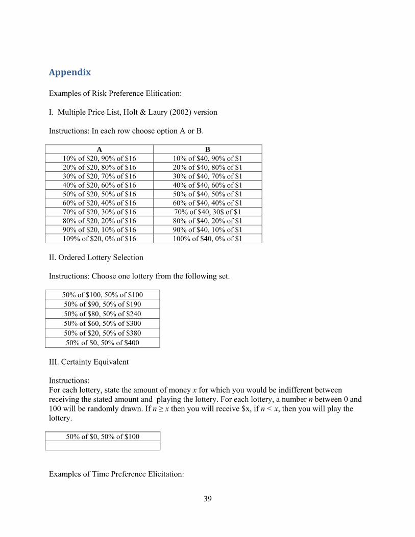
39

AppendixExamples of Risk Preference Elitication: I. Multiple Price List, Holt & Laury (2002) version Instructions: In each row choose option A or B.

A B 10% of $20, 90% of $16 10% of $40, 90% of $1 20% of $20, 80% of $16 20% of $40, 80% of $1 30% of $20, 70% of $16 30% of $40, 70% of $1 40% of $20, 60% of $16 40% of $40, 60% of $1 50% of $20, 50% of $16 50% of $40, 50% of $1 60% of $20, 40% of $16 60% of $40, 40% of $1 70% of $20, 30% of $16 70% of $40, 30$ of $1 80% of $20, 20% of $16 80% of $40, 20% of $1 90% of $20, 10% of $16 90% of $40, 10% of $1 109% of $20, 0% of $16 100% of $40, 0% of $1

II. Ordered Lottery Selection Instructions: Choose one lottery from the following set.

50% of $100, 50% of $100 50% of $90, 50% of $190 50% of $80, 50% of $240 50% of $60, 50% of $300 50% of $20, 50% of $380 50% of $0, 50% of $400

III. Certainty Equivalent Instructions: For each lottery, state the amount of money x for which you would be indifferent between receiving the stated amount and playing the lottery. For each lottery, a number n between 0 and 100 will be randomly drawn. If n ≥ x then you will receive $x, if n < x, then you will play the lottery.

50% of $0, 50% of $100

Examples of Time Preference Elicitation:

40

I. Multiple Price List Instructions: In each row choose option A or B.

A B $100 in 1 week $105 in 1 month $100 in 1 week $110 in 1 month $100 in 1 week $115 in 1 month $100 in 1 week $120 in 1 month $100 in 1 week $125 in 1 month

II. Equivalence Instructions: Fill in the blank with the amount that would be equivalent to you at the given delay. $100 today = $____ in a year III. Willingness to Pay / Willingness to Accept Example 1: How much money would you be willing to accept at the end of this experiment in place of a payment of $10 a week from now? Example 2: How much money would you be willing to pay now in order to receive a payment of $10 a week from now?