1

Measuring Molecular Motion

Using NMR Spectroscopy to Study Translational Diffusion

Jennifer N. Maki and Nikolaus M. Loening*

Department of Chemistry, Lewis & Clark College, Portland, OR 97219

This chapter demonstrates how to use NMR spectroscopy to

measure the rate of translational diffusion. Once measured,

this rate can provide insight into the size and shape of the

molecules in a sample and can even be used to match peaks in

the NMR spectrum with the different components of a sample

mixture. Of the possible applications of diffusion, the

experiment presented focuses on using measurements of the

rate of translational diffusion to reveal how the viscosity of a

solution varies with the concentration of the solutes.

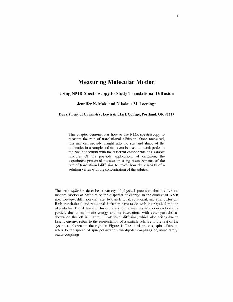
The term diffusion describes a variety of physical processes that involve the

random motion of particles or the dispersal of energy. In the context of NMR

spectroscopy, diffusion can refer to translational, rotational, and spin diffusion.

Both translational and rotational diffusion have to do with the physical motion

of particles. Translational diffusion refers to the seemingly-random motion of a

particle due to its kinetic energy and its interactions with other particles as

shown on the left in Figure 1. Rotational diffusion, which also arises due to

kinetic energy, refers to the reorientation of a particle relative to the rest of the

system as shown on the right in Figure 1. The third process, spin diffusion,

refers to the spread of spin polarization via dipolar couplings or, more rarely,

scalar couplings.

2

The rate at which these processes occur can be measured using NMR

spectroscopy. The rate of spin diffusion can be measured using an NOE build-up

experiment and the rate of rotational diffusion is usually inferred from

measurements of the transverse and longitudinal relaxation rates. The procedure

described in this chapter demonstrates how NMR spectroscopy can be used to

measure the rate of translational diffusion as well as how this rate can provide

insight into the effect of the solute molecules on the bulk properties of the

solution.

Background

In a gas or liquid, the individual molecules have enough kinetic energy to

overcome the intermolecular forces binding them to other molecules in the

sample. Consequently, the molecules move about at a speed determined by their

kinetic energy. As a molecule moves through the sample, it changes direction

and speed due to collisions with other molecules. Over a period of time, the

movement of the molecule forms a zigzag path known as a random walk as

shown on the left side of Figure 1. This movement occurs even in the absence of

external effects (such as concentration gradients or electric fields) and is referred

to as translational diffusion.

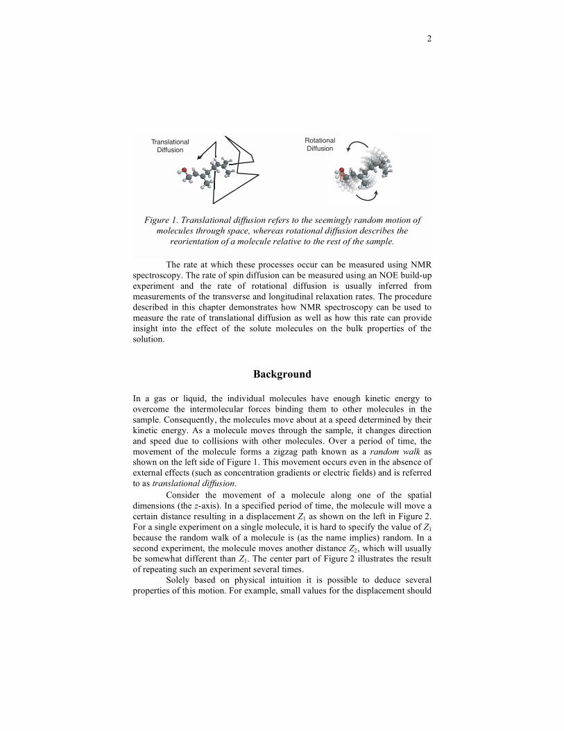
Consider the movement of a molecule along one of the spatial

dimensions (the z-axis). In a specified period of time, the molecule will move a

certain distance resulting in a displacement Z1 as shown on the left in Figure 2.

For a single experiment on a single molecule, it is hard to specify the value of Z1

because the random walk of a molecule is (as the name implies) random. In a

second experiment, the molecule moves another distance Z2, which will usually

be somewhat different than Z1. The center part of Figure 2 illustrates the result

of repeating such an experiment several times.

Solely based on physical intuition it is possible to deduce several

properties of this motion. For example, small values for the displacement should

TranslationalDiffusion

RotationalDiffusion

Figure 1. Translational diffusion refers to the seemingly random motion of

molecules through space, whereas rotational diffusion describes the

reorientation of a molecule relative to the rest of the sample.

3

be more likely than large values since the individual steps of the molecule’s

random walk are more likely to cancel out than to add constructively. Another

property is that, on average, the displacement of the molecules will be zero. This

is because the molecules are just as likely to move in one direction along the z-

axis as the other. Physically, this has to be the case for a stationary sample…if

the average displacement of the molecules was non-zero, than the sample would

be moving rather than stationary. The results of a large number of experiments

(or a large number of molecules in a single experiment) follow a well-defined

trend as shown on the right in Figure 2.

Although it is difficult (if not impossible) to predict the distance that a

single molecule will move in an experiment, it is possible to statistically define

the probability that this molecule will move a certain distance. The statistics of

the random walks of individual particles on the molecular level result in the bulk

property of translational diffusion. The average rate of translational diffusion is

described quantitatively by the diffusion coefficient (D). The value of the

diffusion coefficient depends not only on the identity of the sample molecules,

but also on the solvent and the temperature (and, to a very minor degree, the

pressure). Statistically, the probability for a molecule to be displaced a distance

Z in time t is described by a Gaussian distribution function (1):

P Z( ) =1

4 Dt

expZ

2

4Dt

(1)

Larger diffusion coefficients correspond to more rapid movement of the

molecules; therefore larger displacements are more likely and the distribution

function will be broader. Likewise, larger values of t also result in a broader

distribution function as the molecules have a longer period of time to diffuse.

As expected, the average displacement calculated using eq 1 is zero:

Z = Z P Z( ) dZ = odd function( ) even function( ) = 0

The mean-square displacement, on the other hand, is

Z

2 = Z2P Z( )dZ = 2Dt

Therefore, the root-mean-square displacement for a molecule is

Z

rms= Z

2= 2Dt

The diffusion coefficient is on the order of 1 10–5

cm2 s

–1 for a typical small

molecule in solution, and a typical NMR diffusion measurement experiment is

0.1 s long. These values correspond to a root-mean-square displacement along a

single axis of 14 μm.

4

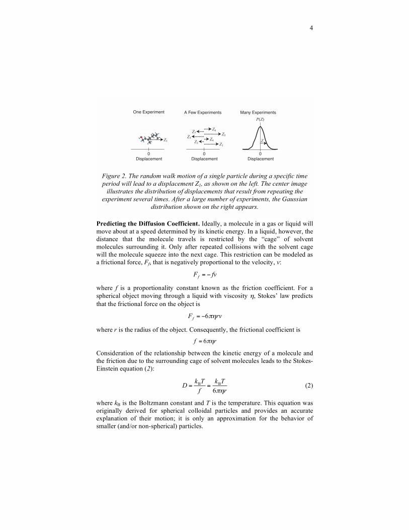
Predicting the Diffusion Coefficient. Ideally, a molecule in a gas or liquid will

move about at a speed determined by its kinetic energy. In a liquid, however, the

distance that the molecule travels is restricted by the “cage” of solvent

molecules surrounding it. Only after repeated collisions with the solvent cage

will the molecule squeeze into the next cage. This restriction can be modeled as

a frictional force, Ff, that is negatively proportional to the velocity, v:

Ff = fv

where f is a proportionality constant known as the friction coefficient. For a

spherical object moving through a liquid with viscosity , Stokes’ law predicts

that the frictional force on the object is

Ff = 6 rv

where r is the radius of the object. Consequently, the frictional coefficient is

f = 6 r

Consideration of the relationship between the kinetic energy of a molecule and

the friction due to the surrounding cage of solvent molecules leads to the Stokes-

Einstein equation (2):

D =

kBT

f=

kBT

6 r (2)

where kB is the Boltzmann constant and T is the temperature. This equation was

originally derived for spherical colloidal particles and provides an accurate

explanation of their motion; it is only an approximation for the behavior of

smaller (and/or non-spherical) particles.

Displacement

A Few Experiments

0

Z1

Displacement

One Experiment Many Experiments

Displacement0

Z1Z4Z2

Z5Z6

Z3Z7

0

P(Z)

Z

Figure 2. The random walk motion of a single particle during a specific time

period will lead to a displacement Z1, as shown on the left. The center image

illustrates the distribution of displacements that result from repeating the

experiment several times. After a large number of experiments, the Gaussian

distribution shown on the right appears.

5

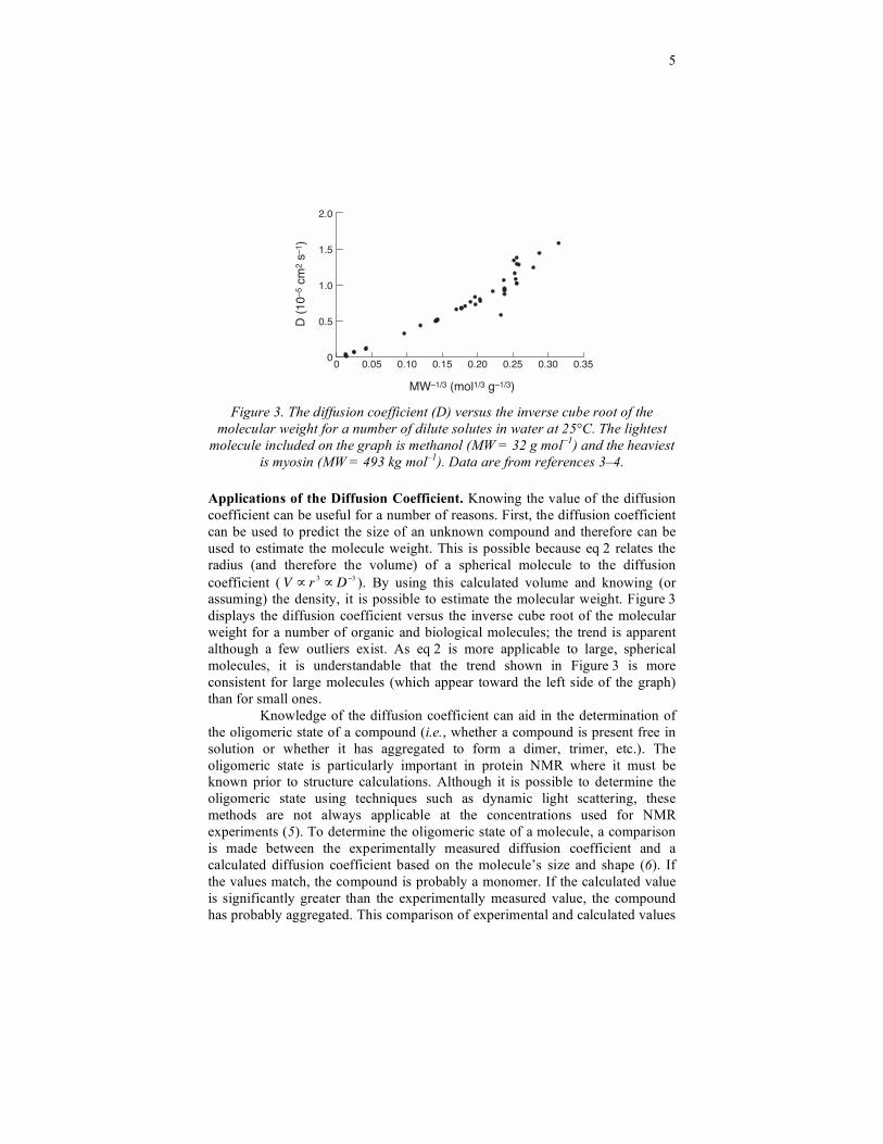
Applications of the Diffusion Coefficient. Knowing the value of the diffusion

coefficient can be useful for a number of reasons. First, the diffusion coefficient

can be used to predict the size of an unknown compound and therefore can be

used to estimate the molecule weight. This is possible because eq 2 relates the

radius (and therefore the volume) of a spherical molecule to the diffusion

coefficient (V r 3 D 3). By using this calculated volume and knowing (or

assuming) the density, it is possible to estimate the molecular weight. Figure 3

displays the diffusion coefficient versus the inverse cube root of the molecular

weight for a number of organic and biological molecules; the trend is apparent

although a few outliers exist. As eq 2 is more applicable to large, spherical

molecules, it is understandable that the trend shown in Figure 3 is more

consistent for large molecules (which appear toward the left side of the graph)

than for small ones.

Knowledge of the diffusion coefficient can aid in the determination of

the oligomeric state of a compound (i.e., whether a compound is present free in

solution or whether it has aggregated to form a dimer, trimer, etc.). The

oligomeric state is particularly important in protein NMR where it must be

known prior to structure calculations. Although it is possible to determine the

oligomeric state using techniques such as dynamic light scattering, these

methods are not always applicable at the concentrations used for NMR

experiments (5). To determine the oligomeric state of a molecule, a comparison

is made between the experimentally measured diffusion coefficient and a

calculated diffusion coefficient based on the molecule’s size and shape (6). If

the values match, the compound is probably a monomer. If the calculated value

is significantly greater than the experimentally measured value, the compound

has probably aggregated. This comparison of experimental and calculated values

D (

10–5

cm

2 s–

1 )

MW–1/3 (mol1/3 g–1/3)

0 0.05 0.10 0.15 0.20 0.25 0.30 0.350

0.5

1.0

1.5

2.0

Figure 3. The diffusion coefficient (D) versus the inverse cube root of the

molecular weight for a number of dilute solutes in water at 25°C. The lightest

molecule included on the graph is methanol (MW = 32 g mol–1

) and the heaviest

is myosin (MW = 493 kg mol–1

). Data are from references 3–4.

6

is most useful for detecting dimerization, as the molecular weights of a

monomer and a dimer differ by a factor of two. Differentiating higher

oligomeric states, such as whether a molecule is a trimer or a tetramer, becomes

progressively more difficult as the ratio of the molecular weights (and therefore

the variations in the diffusion coefficients) will be smaller. This method is most

applicable to large molecules, such as proteins, but also has been used for

smaller systems such as non-covalent assemblies of calix[4]arene units (6) and

ions in solution (7).

Similarly, diffusion coefficients can be used to estimate binding

affinities between substrates and proteins. For example, one screening method

used in drug discovery is to observe how the apparent diffusion coefficient for a

small molecule changes in the presence of a protein. A decline in the diffusion

coefficient of the small molecule in the presence of a protein is indicative of

binding, in which case the small molecule is a good candidate for a drug. As will

be seen later in this chapter, it is important in such experiments to control for

changes in the viscosity upon addition of further solute or other solutes as the

solution viscosity, and consequently the diffusion coefficients, is very sensitive

to the composition of the sample.

Measurements of the diffusion coefficients can also be used to separate

signals from different molecules. In NMR spectroscopy, the spectrum of a

mixture is equivalent to the superposition of the spectra of the individual

components. Using the experiment described later in this chapter, it is possible

to measure a diffusion coefficient for each peak in the spectrum. As the peaks

from the non-exchangeable nuclei of a compound will share the same diffusion

coefficient, it is possible to use the diffusion coefficient to distinguish signals

from different components of the mixture (provided they have appreciably

different diffusion coefficients). This method of separating signals is known as

diffusion-ordered spectroscopy, or DOSY (8). DOSY is particularly useful in

situations where it is not convenient or possible to physically separate a mixture;

DOSY is capable of separating the signals from different components without

the need to resort to chromatography. Another use for DOSY is in cases where it

is the mixture of components and their interactions that is of interest.

Magnetic Field Gradients and NMR Spectroscopy

Before running an NMR experiment, it is typical to spend some time

“shimming” the magnet. The shimming procedure is carried out in order to

make the magnetic field as homogeneous as possible; this is necessary because

spatial inhomogeneities in the main magnetic field interfere with the resolution

of the NMR experiment. However, observing translational diffusion by NMR

spectroscopy requires a spatially-dependent magnetic field. In other words, it is

7

necessary to reintroduce inhomogeneities to the main magnetic field to measure

the diffusion coefficient.

Experimentally, these inhomogeneities are generated using gradients.

Gradients are coils inside the NMR probe that generate well-defined spatial

variations of the magnetic field. Most gradients are designed to generate a linear

variation in the magnetic field along the axis of the main magnetic field (B0);

this axis is usually defined as the z-axis and therefore such a gradient is called a

z-axis gradient. The symbol Gz represents the strength of such a gradient

[Gz = B(z)/ z]. By changing the magnitude and sign of the electrical current

running through the coil of the gradient it is possible to vary the magnitude and

the sign of Gz. Likewise, the gradient can be switched off (Gz = 0) by switching

off the electrical current.

Although z-axis gradients are the most common type of magnetic field

gradients, it is possible to generate gradients along other axes, such as the x-axis,

the y-axis, or even along the rotor axis of a magic-angle spinning probe. In a

typical NMR probe, each gradient coil can generate a magnetic field gradient of

several tens of Gauss cm–1

for a period of several milliseconds (a “gradient

pulse”); weaker gradient pulses can be generated for much longer periods. In all

cases, the direction of the magnetic field generated by the gradient is parallel to

B0; the gradient axis is the axis along which the magnitude, not the direction, of

the field varies.

Magnetization and Gradients. The Larmor frequency ( ) for the nuclei in a

sample depends on the magnetic field and the magnetogyric ratio ( ):

= B

0

When a gradient is applied, the magnetic field varies linearly along the gradient

axis and, consequently, the Larmor frequency varies in the same way. As a

result, nuclei at different parts of the sample will precess at different

frequencies. On a bulk scale, the result is a spatially-dependent phase for the

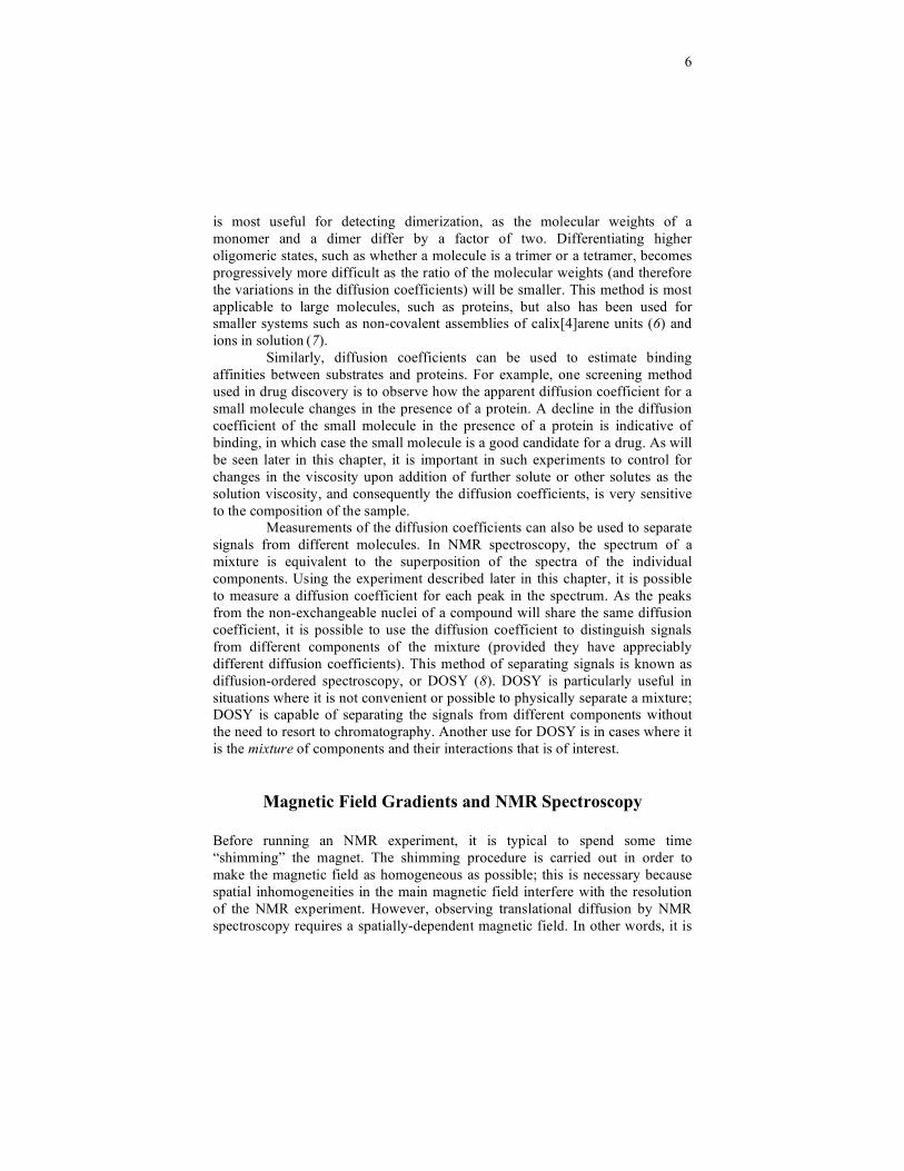
transverse sample magnetization. As shown in Figure 4, the magnetization will

begin to vary in phase across the sample after the gradient is switched on,

resulting in a helical profile for the transverse magnetization along the gradient

axis. As the signal observed in the NMR experiment arises from the sum of all

the transverse magnetization in the sample, the spatially-dependent phase results

in a diminished signal because the transverse (x and y) components of the

magnetization will tend to cancel one another. The degree to which the signal is

diminished depends on how tightly the transverse magnetization is “coiled”

along the gradient axis. This signal attenuation due to a gradient pulse is referred

to as gradient dephasing.

Consider an experiment in which two gradient pulses are applied. The

first gradient pulse, often referred to as the phase-labeling gradient, dephases

any transverse magnetization. A second gradient pulse can be used to reverse

8

this process if the appropriate combination of pulse length and strength are used.

Such a gradient is called a refocusing gradient because it uncoils the

magnetization helix and restores the transverse magnetization to its initial state.

For the magnetization to be properly refocused, the gradient values must be

chosen such that the spatially dependent phase sums to zero at the end of the

experiment. By carefully choosing the strengths of different gradients in an

experiment, it is possible to use gradients in place of phase cycling for selecting

different components of the NMR signal. However, this is not the focus of this

chapter; instead, we will concentrate on how gradients are used to measure

translational diffusion.

Gradients and Motion. The measurement of motion by NMR requires at least

two gradient pulses in an experiment: the first to dephase the magnetization and

the second to refocus it at some later point in the experiment. To completely

refocus the magnetization (and completely recover the NMR signal), the

molecules of the sample must not move during the time period in between the

gradients. If the molecules do move, the observed signal will change because the

refocusing gradient will not be able to properly restore the transverse

magnetization to its initial phase.

In order to visualize how movement affects the result of a gradient-

selected experiment it is useful to consider a discrete version of the

magnetization helix shown in Figure 4. In the discrete model (shown in

Figure 5), the sample is split into thin slices referred to as isochromats in which

the magnetic field is approximately homogeneous. Before the first gradient

pulse the components of the magnetization in the various isochromats are

aligned as shown on the left in Figure 5. During the gradient, the nuclei precess

at different frequencies in each isochromat. This variation in precession results

in the situation shown on the right of Figure 5. In the absence of motion, a

suitable refocusing gradient will realign the magnetization. However, if the

nuclei move in between the phase-labeling and refocusing gradients, the signal

z

x y

Figure 4. A gradient pulse along the z-axis winds the transverse magnetization

into a “helix” (the helix traces out the tips of the magnetization vectors). The

pitch of this helix (i.e., how tightly it is wound) depends on the gradient strength

and length, and the magnetogyric ratio of the nuclei.

9

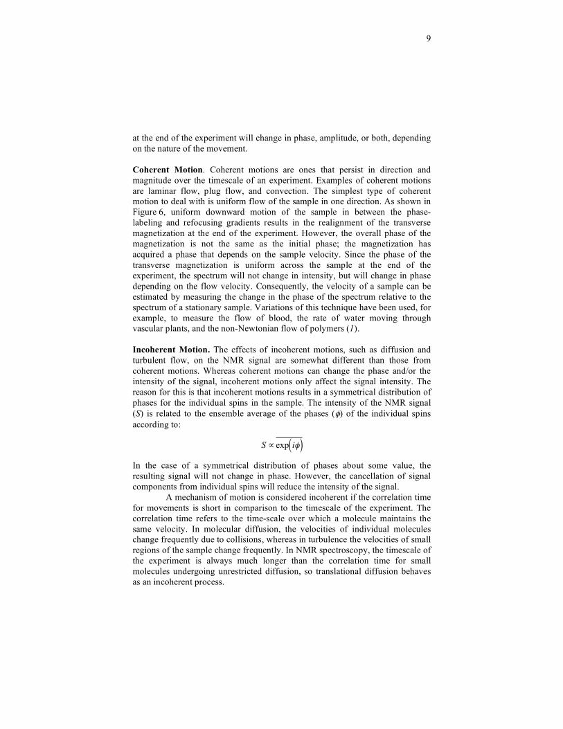
at the end of the experiment will change in phase, amplitude, or both, depending

on the nature of the movement.

Coherent Motion. Coherent motions are ones that persist in direction and

magnitude over the timescale of an experiment. Examples of coherent motions

are laminar flow, plug flow, and convection. The simplest type of coherent

motion to deal with is uniform flow of the sample in one direction. As shown in

Figure 6, uniform downward motion of the sample in between the phase-

labeling and refocusing gradients results in the realignment of the transverse

magnetization at the end of the experiment. However, the overall phase of the

magnetization is not the same as the initial phase; the magnetization has

acquired a phase that depends on the sample velocity. Since the phase of the

transverse magnetization is uniform across the sample at the end of the

experiment, the spectrum will not change in intensity, but will change in phase

depending on the flow velocity. Consequently, the velocity of a sample can be

estimated by measuring the change in the phase of the spectrum relative to the

spectrum of a stationary sample. Variations of this technique have been used, for

example, to measure the flow of blood, the rate of water moving through

vascular plants, and the non-Newtonian flow of polymers (1).

Incoherent Motion. The effects of incoherent motions, such as diffusion and

turbulent flow, on the NMR signal are somewhat different than those from

coherent motions. Whereas coherent motions can change the phase and/or the

intensity of the signal, incoherent motions only affect the signal intensity. The

reason for this is that incoherent motions results in a symmetrical distribution of

phases for the individual spins in the sample. The intensity of the NMR signal

(S) is related to the ensemble average of the phases ( ) of the individual spins

according to:

S exp i( )

In the case of a symmetrical distribution of phases about some value, the

resulting signal will not change in phase. However, the cancellation of signal

components from individual spins will reduce the intensity of the signal.

A mechanism of motion is considered incoherent if the correlation time

for movements is short in comparison to the timescale of the experiment. The

correlation time refers to the time-scale over which a molecule maintains the

same velocity. In molecular diffusion, the velocities of individual molecules

change frequently due to collisions, whereas in turbulence the velocities of small

regions of the sample change frequently. In NMR spectroscopy, the timescale of

the experiment is always much longer than the correlation time for small

molecules undergoing unrestricted diffusion, so translational diffusion behaves

as an incoherent process.

10

z

Initially After Gradient

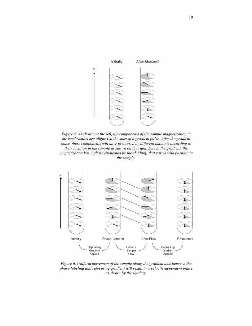
Figure 5. As shown on the left, the components of the sample magnetization in

the isochromats are aligned at the start of a gradient pulse. After the gradient

pulse, these components will have precessed by different amounts according to

their location in the sample as shown on the right. Due to the gradient, the

magnetization has a phase (indicated by the shading) that varies with position in

the sample.

z

Initially Phase-Labeled After Flow Refocused

DephasingGradientApplied

RephasingGradientApplied

UniformSample

Flow Figure 6. Uniform movement of the sample along the gradient axis between the

phase-labeling and refocusing gradient will result in a velocity-dependent phase

as shown by the shading.

11

Measuring Diffusion Coefficients

A Gaussian distribution function (eq 1) describes the distribution of molecular

displacements due to translational diffusion. Therefore, in an NMR experiment

with dephasing and refocusing gradients there will be a Gaussian distribution of

phases due to translational diffusion between these two gradients pulses. As this

Gaussian distribution of phases is symmetric the effect of molecular diffusion in

the NMR experiment is only to attenuate the signal; diffusion does not cause the

signal to change in phase. The degree to which diffusion attenuates the signal

can be calculated based on a modified version of the Bloch equations (which are

a set of differential equations that provide a semi-classical description of the

NMR experiment). The result of this derivation (9) is that the attenuation of the

signal (S) relative to the signal in the absence of diffusion (S0) is

S = S0 exp D

2G

2 2s

2 13( )[ ] (3)

where is the magnetogyric ratio, G is the gradient strength, is the length of

the gradient pulses, is the time between the gradients, and s is a shape factor

which accounts for how the gradient pulses are ramped on and off. Typically, s

will be either 1 (for rectangular-shaped gradient pulses) or 2/ (for half-sine bell

shaped gradient pulses) (10). If we take the natural log of this equation, we find

ln S = ln S

0D

2G

2 2s

2 1

3( ) (4)

Consequently, a plot of –ln S versus

2G

2

2s

2 ( –

1/3 ) should result in a straight

line with slope D and y-intercept –ln S0. One subtle point for using eq 4 is that,

when linear regression is used to fit the data, all the points are weighted equally.

This can yield inaccurate results, as noise will disproportionately affect some of

the data. This problem is not severe if the signal-to-noise ratio for all the data is

good; if this is not the case then directly fitting the data to eq 3 using a non-

linear fit yields more accurate results (11).

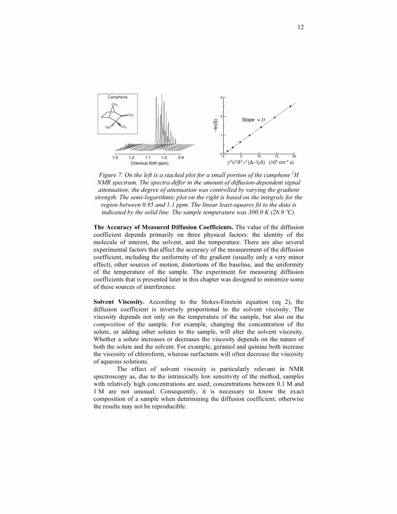
Figure 7 illustrates the diffusion-dependent signal attenuation for a

sample of camphene in deuterated methanol in a series of experiments with

increasing gradient strength. The spectra were integrated between 1.1 and

0.95 ppm and, as shown on the right of Figure 7, the integrals were plotted

versus

2G

2

2s

2 ( –

1/3 ) using a semi-log plot. The slope of this plot

corresponds to the diffusion coefficient. For this sample, linear least-squares was

used to fit the data, resulting in an estimated diffusion coefficient of

1.339 (±0.002) 10–5

cm2 s

–1. The quoted error is the standard deviation of the

slope resulting from the linear regression analysis, which usually underestimates

the experimental error inherent in the technique. This value for the diffusion

coefficient was deduced using the integrals of the methyl peaks; other camphene

peaks in the spectrum should provide identical results.

12

The Accuracy of Measured Diffusion Coefficients. The value of the diffusion

coefficient depends primarily on three physical factors: the identity of the

molecule of interest, the solvent, and the temperature. There are also several

experimental factors that affect the accuracy of the measurement of the diffusion

coefficient, including the uniformity of the gradient (usually only a very minor

effect), other sources of motion, distortions of the baseline, and the uniformity

of the temperature of the sample. The experiment for measuring diffusion

coefficients that is presented later in this chapter was designed to minimize some

of these sources of interference.

Solvent Viscosity. According to the Stokes-Einstein equation (eq 2), the

diffusion coefficient is inversely proportional to the solvent viscosity. The

viscosity depends not only on the temperature of the sample, but also on the

composition of the sample. For example, changing the concentration of the

solute, or adding other solutes to the sample, will alter the solvent viscosity.

Whether a solute increases or decreases the viscosity depends on the nature of

both the solute and the solvent. For example, geraniol and quinine both increase

the viscosity of chloroform, whereas surfactants will often decrease the viscosity

of aqueous solutions.

The effect of solvent viscosity is particularly relevant in NMR

spectroscopy as, due to the intrinsically low sensitivity of the method, samples

with relatively high concentrations are used; concentrations between 0.1 M and

1 M are not unusual. Consequently, it is necessary to know the exact

composition of a sample when determining the diffusion coefficient; otherwise

the results may not be reproducible.

1.0 1.3 1.2 1.1 Chemical Shift (ppm)

0 5 10 15 20 0

1

2

3

–ln(

S)

0.9

Slope = D

2G

2 2 s

2 (Δ–1/3 ) (105 cm–2 s)γ δ δ

H 2 C

C H 2

C H 3 H 3 C

Camphene

Figure 7. On the left is a stacked plot for a small portion of the camphene 1H

NMR spectrum. The spectra differ in the amount of diffusion-dependent signal

attenuation; the degree of attenuation was controlled by varying the gradient

strength. The semi-logarithmic plot on the right is based on the integrals for the

region between 0.95 and 1.1 ppm. The linear least-squares fit to the data is

indicated by the solid line. The sample temperature was 300.0 K (26.9 ºC).

13

Restricted Diffusion. The theory used to derive eqs 1 and 3 assumes that the

movement of the sample molecules is unbounded. If this is not the case, then the

molecules are subject to restricted diffusion and the signal attenuation due to

diffusion will be less than what eq 3 predicts. Fortunately, a typical solution-

state NMR sample tube has a diameter of several millimeters whereas the

sample molecules move only a few tens of micrometers during an experiment.

Therefore, the effect due to restricted diffusion can be safely ignored and eqs 1,

3, and 4 can be used without difficulty.

Motion. NMR experiments involving gradient pulses are sensitive to both

coherent and incoherent motions. This means that any attempt to measure the

diffusion coefficient in the presence of another source of movement produces

results that reflect both movements. Consequently, diffusion measurements

should be performed without sampling spinning.

In addition, convection can arise due to small temperature gradients in

the sample; this is particularly common for low viscosity solvents such as

chloroform or acetone (12). In diffusion-measurement experiments, sample

convection introduces an additional component to the signal decay that results in

overestimates of the diffusion coefficient. Fortunately, convection is, at least to a

first approximation, a coherent motion and therefore the signal variation due to

convection can be removed by using the double-stimulated echo experiment

described later in this chapter (13).

Gradient Calibration. To make accurate measurements of the diffusion

coefficient, an accurate value for the strength of the gradient needs to be known.

Typically, this value will be determined when the NMR system is installed and

is unlikely to need to be recalibrated. If the value is unknown, it can be

determined in two ways. The first method involves making a diffusion

measurement using a sample with a known diffusion coefficient. By working

backwards from the known diffusion coefficient, it is possible to determine the

strength of the gradient.

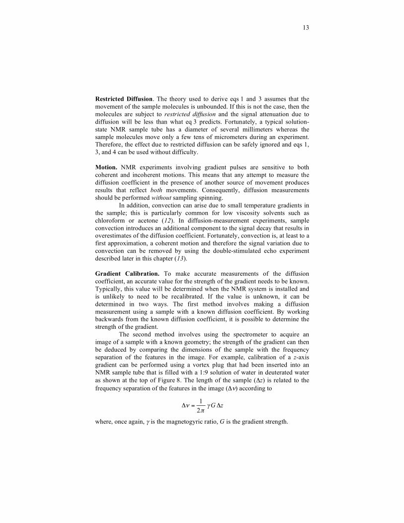
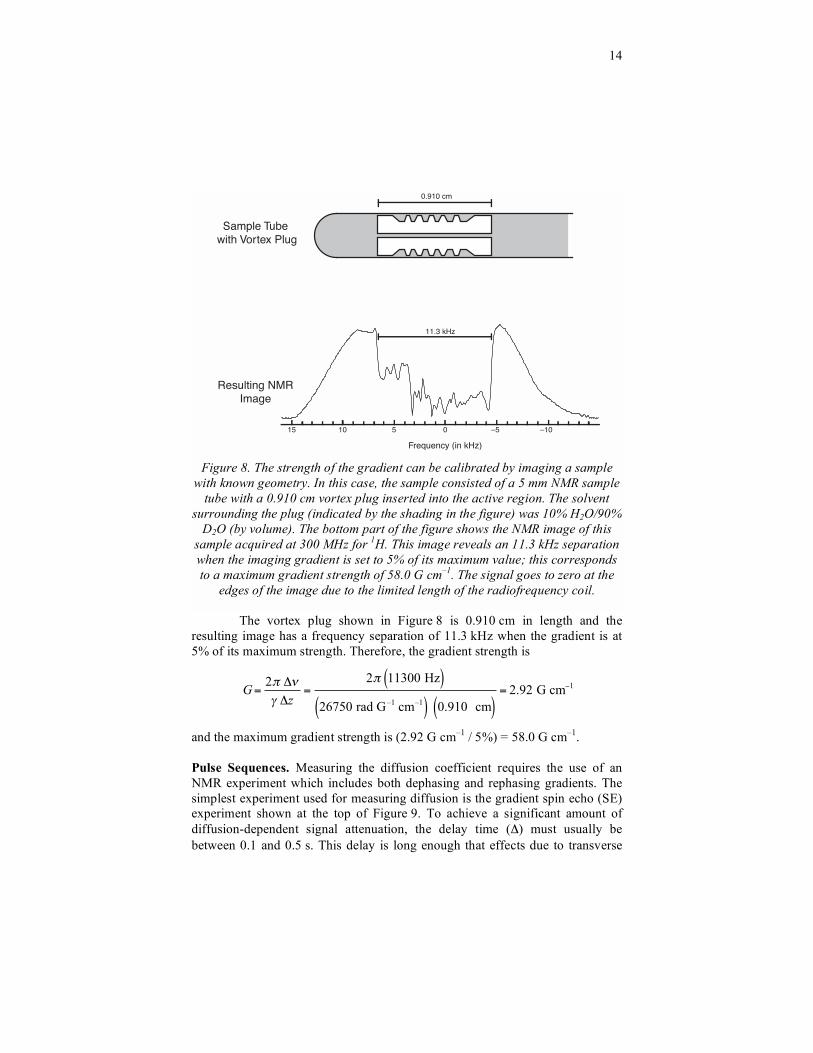
The second method involves using the spectrometer to acquire an

image of a sample with a known geometry; the strength of the gradient can then

be deduced by comparing the dimensions of the sample with the frequency

separation of the features in the image. For example, calibration of a z-axis

gradient can be performed using a vortex plug that had been inserted into an

NMR sample tube that is filled with a 1:9 solution of water in deuterated water

as shown at the top of Figure 8. The length of the sample ( z) is related to the

frequency separation of the features in the image ( ) according to

=1

2G z

where, once again, is the magnetogyric ratio, G is the gradient strength.

14

The vortex plug shown in Figure 8 is 0.910 cm in length and the

resulting image has a frequency separation of 11.3 kHz when the gradient is at

5% of its maximum strength. Therefore, the gradient strength is

G =2

z=

2 11300 Hz( )

26750 rad G–1

cm–1( ) 0.910 cm( )

= 2.92 G cm1

and the maximum gradient strength is (2.92 G cm–1

/ 5%) = 58.0 G cm–1

.

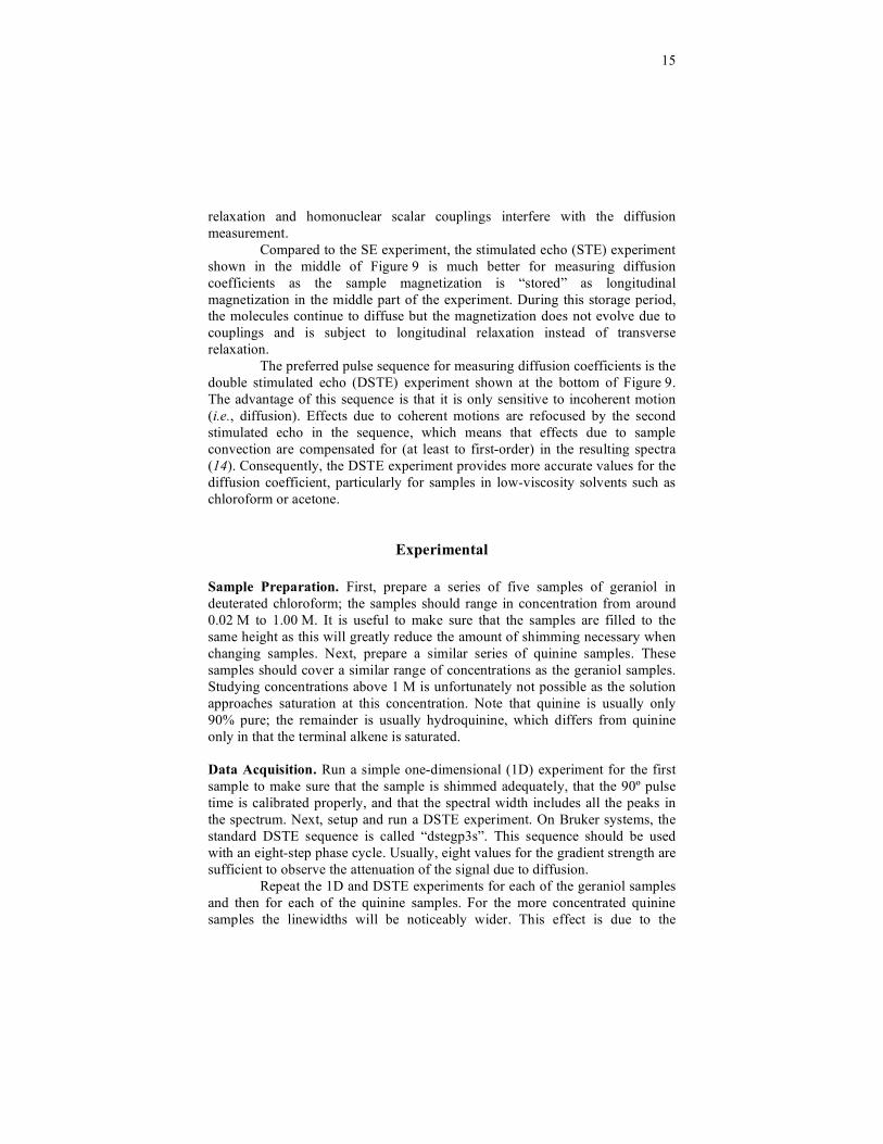
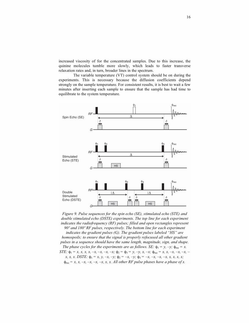
Pulse Sequences. Measuring the diffusion coefficient requires the use of an

NMR experiment which includes both dephasing and rephasing gradients. The

simplest experiment used for measuring diffusion is the gradient spin echo (SE)

experiment shown at the top of Figure 9. To achieve a significant amount of

diffusion-dependent signal attenuation, the delay time ( ) must usually be

between 0.1 and 0.5 s. This delay is long enough that effects due to transverse

Frequency (in kHz)

11.3 kHz

0.910 cm

Sample Tube with Vortex Plug

Resulting NMRImage

–10–515 10 5 0

Figure 8. The strength of the gradient can be calibrated by imaging a sample

with known geometry. In this case, the sample consisted of a 5 mm NMR sample

tube with a 0.910 cm vortex plug inserted into the active region. The solvent

surrounding the plug (indicated by the shading in the figure) was 10% H2O/90%

D2O (by volume). The bottom part of the figure shows the NMR image of this

sample acquired at 300 MHz for 1H. This image reveals an 11.3 kHz separation

when the imaging gradient is set to 5% of its maximum value; this corresponds

to a maximum gradient strength of 58.0 G cm–1

. The signal goes to zero at the

edges of the image due to the limited length of the radiofrequency coil.

15

relaxation and homonuclear scalar couplings interfere with the diffusion

measurement.

Compared to the SE experiment, the stimulated echo (STE) experiment

shown in the middle of Figure 9 is much better for measuring diffusion

coefficients as the sample magnetization is “stored” as longitudinal

magnetization in the middle part of the experiment. During this storage period,

the molecules continue to diffuse but the magnetization does not evolve due to

couplings and is subject to longitudinal relaxation instead of transverse

relaxation.

The preferred pulse sequence for measuring diffusion coefficients is the

double stimulated echo (DSTE) experiment shown at the bottom of Figure 9.

The advantage of this sequence is that it is only sensitive to incoherent motion

(i.e., diffusion). Effects due to coherent motions are refocused by the second

stimulated echo in the sequence, which means that effects due to sample

convection are compensated for (at least to first-order) in the resulting spectra

(14). Consequently, the DSTE experiment provides more accurate values for the

diffusion coefficient, particularly for samples in low-viscosity solvents such as

chloroform or acetone.

Experimental

Sample Preparation. First, prepare a series of five samples of geraniol in

deuterated chloroform; the samples should range in concentration from around

0.02 M to 1.00 M. It is useful to make sure that the samples are filled to the

same height as this will greatly reduce the amount of shimming necessary when

changing samples. Next, prepare a similar series of quinine samples. These

samples should cover a similar range of concentrations as the geraniol samples.

Studying concentrations above 1 M is unfortunately not possible as the solution

approaches saturation at this concentration. Note that quinine is usually only

90% pure; the remainder is usually hydroquinine, which differs from quinine

only in that the terminal alkene is saturated.

Data Acquisition. Run a simple one-dimensional (1D) experiment for the first

sample to make sure that the sample is shimmed adequately, that the 90º pulse

time is calibrated properly, and that the spectral width includes all the peaks in

the spectrum. Next, setup and run a DSTE experiment. On Bruker systems, the

standard DSTE sequence is called “dstegp3s”. This sequence should be used

with an eight-step phase cycle. Usually, eight values for the gradient strength are

sufficient to observe the attenuation of the signal due to diffusion.

Repeat the 1D and DSTE experiments for each of the geraniol samples

and then for each of the quinine samples. For the more concentrated quinine

samples the linewidths will be noticeably wider. This effect is due to the

16

increased viscosity of for the concentrated samples. Due to this increase, the

quinine molecules tumble more slowly, which leads to faster transverse

relaxation rates and, in turn, broader lines in the spectrum.

The variable temperature (VT) control system should be on during the

experiments. This is necessary because the diffusion coefficients depend

strongly on the sample temperature. For consistent results, it is best to wait a few

minutes after inserting each sample to ensure that the sample has had time to

equilibrate to the system temperature.

HS HS

HSG

RFStimulatedEcho (STE)

G

RFDouble Stimulated Echo (DSTE)

12

12

G

RFSpin Echo (SE)

Figure 9. Pulse sequences for the spin echo (SE), stimulated echo (STE) and

double stimulated echo (DSTE) experiments. The top line for each experiment

indicates the radiofrequency (RF) pulses; filled and open rectangles represent

90º and 180º RF pulses, respectively. The bottom line for each experiment

indicates the gradient pulses (G). The gradient pulses labeled “HS” are

homospoils; to ensure that the signal is properly refocused all other gradient

pulses in a sequence should have the same length, magnitude, sign, and shape.

The phase cycles for the experiments are as follows. SE: 1 = y, –y; rec = x.

STE: 1 = x, x, x, x, –x, –x, –x, –x; 2 = 3 = y, –y, x, –x; rec = x, x, –x, –x, –x, –

x, x, x. DSTE: 1 = x, y, –x, –y; 2 = –x, –y; 3 = –x, –x, –x, –x, x, x, x, x;

rec = x, x, –x, –x, –x, –x, x, x. All other RF pulse phases have a phase of x.

17

Data Processing. Once acquired, each DSTE experiment should be phased and

Fourier transformed in the directly-detected dimension. It is usually a good idea

to baseline correct the spectra as baseline errors generate systematic errors in the

calculated diffusion coefficients. Next, select a region and integrate each of the

rows in the data set. Usually, the best region to use is one that has a strong signal

and that is well removed from solvent and impurity peaks. For geraniol, the

methyl region (1.8 – 1.5 ppm) works well. For quinine, one of the peaks in the

aromatic region (8.5 –7 ppm) or the methyl peak at ~3.8 ppm are suggested.

On Bruker spectrometers running XWIN-NMR the analysis of the data

can be performed using the relaxation (t1/t2) environment. However, the

interface for this function is somewhat Byzantine, so we use a program

developed by one of the authors to integrate each row (14) and then analyze the

data using a separate program.

Once measured, the integrals should be fit to eq 4 using linear

regression (or to eq 3 using a non-linear fitting routine) to determine the

diffusion coefficients. For our data, we fit the data to eq 3 using the solver

macro in Excel.

Results and Discussion

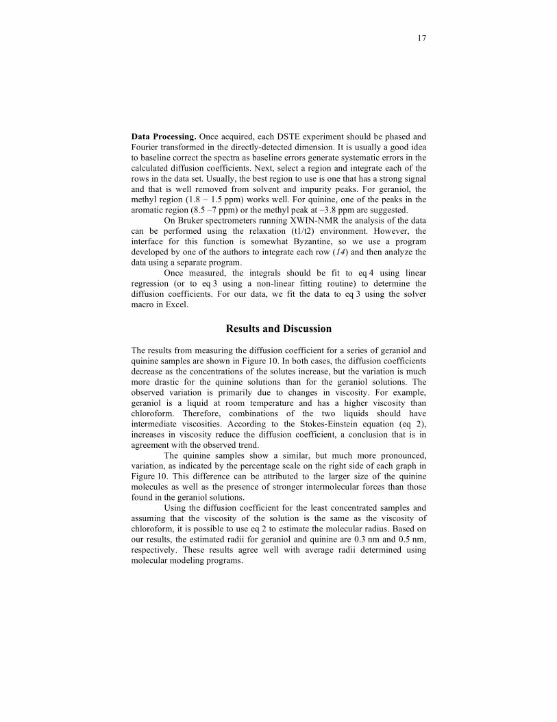
The results from measuring the diffusion coefficient for a series of geraniol and

quinine samples are shown in Figure 10. In both cases, the diffusion coefficients

decrease as the concentrations of the solutes increase, but the variation is much

more drastic for the quinine solutions than for the geraniol solutions. The

observed variation is primarily due to changes in viscosity. For example,

geraniol is a liquid at room temperature and has a higher viscosity than

chloroform. Therefore, combinations of the two liquids should have

intermediate viscosities. According to the Stokes-Einstein equation (eq 2),

increases in viscosity reduce the diffusion coefficient, a conclusion that is in

agreement with the observed trend.

The quinine samples show a similar, but much more pronounced,

variation, as indicated by the percentage scale on the right side of each graph in

Figure 10. This difference can be attributed to the larger size of the quinine

molecules as well as the presence of stronger intermolecular forces than those

found in the geraniol solutions.

Using the diffusion coefficient for the least concentrated samples and

assuming that the viscosity of the solution is the same as the viscosity of

chloroform, it is possible to use eq 2 to estimate the molecular radius. Based on

our results, the estimated radii for geraniol and quinine are 0.3 nm and 0.5 nm,

respectively. These results agree well with average radii determined using

molecular modeling programs.

18

We measured the viscosity of solutions of geraniol and quinine in

chloroform at concentrations ranging from 0 to 1 M using an Ostwald

viscometer. Based on these results and our estimated molecular radii, we used

eq 2 to calculate the variation of the diffusion coefficient with concentration.

These “theoretical” diffusion coefficients are shown as gray lines in Figure 10.

The close correspondence between the experimental diffusion coefficients and

the calculated values indicate that the sample viscosity is the primary reason for

the observed variation in the diffusion coefficients.

Conclusion

NMR spectroscopy is a powerful technique for measuring molecular motion

since the technique is non-invasive and does not require physically “tagging” the

sample. The rate of translational diffusion can be easily measured in a relatively

short NMR experiment, and this information can be used to make inferences

about the size of the sample molecules as well as to observe the effect of the

0 0.2 0.4 0.6 0.8 1 1.20

0.2

0.4

0.6

0.8

Quinine Concentration (M)

0%

20%

40%

60%

80%

100%

0

0.4

0.8

1.2

0 0.2 0.4 0.6 0.8 1 1.2

Geraniol Concentration (M)

Diff

usio

n C

oeffi

cien

t (10

–5 c

m2

s–1 )

0%

20%

40%

60%

80%

100%

CH3

CH3HO

CH3

N

H2C

N

OH3C

HOH

HQuinine

Geraniol

Figure 10. Experimental results for the measurement of the diffusion coefficients

for a series of geraniol samples (on left) and a series of quinine samples (on

right). The right axis on each graph shows the percent change (100%

corresponds to the diffusion coefficient for the least concentrated sample). The

data were acquired on a Bruker NMR spectrometer operating at 300 MHz for 1H. At each concentration, seven (geraniol) or nine (quinine) distinct peaks were

integrated and fit to determine the diffusion coefficient. The data represent the

average value for each concentration along with the standard deviation. The

gray lines indicate “theoretical” values of the diffusion coefficients predicted

using eq 2 as explained in the text. The sample temperature was maintained at

300.0 K (26.9 ºC) throughout the diffusion measurement experiments.

19

solutes on the bulk properties of the solution. Additionally, measurements of the

diffusion coefficients can provide insights into the oligomeric state of molecules

or be used to monitor protein-ligand binding. However, as the results of such

measurements are highly dependent on the sample composition, temperature,

and solvent viscosity, these influences need to be included in any interpretation

of the diffusion coefficients.

References

1. Callaghan, P. T. Principles of Nuclear Magnetic Resonance Microscopy;

Oxford Science Publications: Oxford, UK, 1991; Chapter 6, pp 333.

2. Chang, P. T. Physical Chemistry for the Chemical and Biological Sciences,

2nd

ed.; University Science Books: Sausalito, CA, 2000; Chapter 21, pp 881.

3. Longsworth, L. G., J. Chem. Phys. 1954, 58, 770.

4. Mortimer, R. G. Physical Chemistry; The Benjamin/Cummings Publishing

Company: Redwood City, CA, 1993; Appendix A, pp A-24.

5. Krishnan, V. V. J. Magn. Reson. 1997, 124, 468.

6. Timmerman, P.; Weidmann, J. L.; Jolliffe, K. A.; Prins, L. J.; Reinhoudt, D.

N.; Shinkai, S.; Frish, L.; Cohen, Y. J. Chem. Soc. Perk. T. 2 2000, 10,

2077.

7. Mo, H. P.; Pochapsky, T. C. J. Phys. Chem. B 1997, 101, 4485.

8. Morris, K. F.; Johnson, C. S., Jr. J. Am. Chem. Soc. 1992, 114, 3139.

9. Stejskal, E. O.; Tanner, J. E. J. Chem. Phys. 1965, 42, 288.

10. An additional small correction should be introduced to eqs 3 and 4 to

further compensate for the shape factor, but in most cases this is negligible.

For more information, see Price, W. S.; Kuchel, P. W. J. Magn. Reson..

1990, 94, 133.

11. Johnson, C. S., Jr. Prog. in NMR Spectrosc. 1999, 34, 203.

12. Loening, N. M.; Keeler, J. J. Magn. Reson. 1999, 139, 334.

13. Jerschow, A.; Müller, N. M. J. Magn. Reson. 1997, 125, 372.

14. The integration routine (which works from within XWIN-NMR or

TOPSPIN) can be downloaded from the author’s website at: http://www.lclark.edu/~loening/software/introws