Embed Size (px)
Citation preview
ELSEVIER Journal of Financial Economics 43 (1997)301 339 E C O N O M I C S
Measuring long-horizon security price performance S.P. Kothari*, Jerold B. Warner
William E. Simon Graduate School (?['Business Administration, UniversiO' of Rochester, Rochester, NY 14627. USA
iReccived January 1996; final version received August 1996)
Abstract
Our simulation results show that tests for long-horizon (i.e., multi-year) abnormal security returns around firm-specific events are severely misspecified. The rejection frequencies using parametric tests sometimes exceed 30% when the significance level of the test is 5°A,. Our results are robust to many different abnormal-return models. Conclusions from long-horizon studies require extreme caution. Nonparametr ic and bootstrap tests are likely to reduce misspecification.
Key words: Event studies; Long-horizon performance; Abnormal returns J E L class
302 XP. Kothari, .LB. Warner/Journal of kTnancial Economics 43 (1997) 301 339
Long-horizon tests focusing on pre-event periods are important for understand- ing whether unusual performance preceded or caused an event. Tests for post-event abnormal performance provide evidence on market efficiency. A rap- idly growing literature suggests delayed stock price reaction to at least a dozen events, with abnormal performance apparently persisting for years following events. As surveyed later, the events include repurchase tender offers (Lakonishok and Vermaelen, 1990), spinoffs (Cusatis, Miles, and Woolridge, 1993; Hite and Owers, 1983), dividend initiations (Michaely, Thaler, and Womack, 1995), open market repurchases (Ikenberry, Lakonishok, and Ver- maelen, 1995), stock splits (Desai and Jain, 1995; Ikenberry, Rankine, and Stice, 1996), initial public offerings (e.g., Ritter, 1991), proxy contests (lkenberry and Lakonishok, 1993}, seasoned equity offerings (e.g., Speiss and Affleck-Graves, 1995), short interest announcements (e.g., Asquith and Meulbroek, 1995), NYSE/AMEX listing of the firm's common stock (Dharan and Ikenberry, 1995), dividend omissions (Michaely, Thaler, and Womack, 1995), and mergers (Jensen and Ruback, 1983; Agrawal, Jaffe, and Mandelker, 1992).
Our main result is that long-horizon tests are misspecified. For example, in samples of 200 securities, procedures based on the Fama French three-factor model show abnormal performance over a 36-month horizon for 34.8% of the samples, using two-tailed parametric tests at the 5% significance level. The results are similar using other procedures and the general conclusions are not sensitive to the specific performance benchmarks. Further, the tests can show both positive and negative abnormal performance too often. Moreover, the abnormal perfor- mance persists throughout the horizon following a simulated event.
The persistence of both positive and negative abnormal performance follow- ing simulated events is also a regularity we identify in our survey of the long-horizon literature. This raises the possibility that previous findings are due to test misspecification rather than mispricing. At a minimum, conclusions from existing long-horizon studies require extreme caution. This warning is rein- forced in an independent simulation study by Barber and Lyon (1996a), who also find that many commonly used long-horizon tests are misspecified. Further, both our findings and Barber and Lyon (1996b) indicate that the direction and magnitude of bias in long-horizon studies can be sensitive to sample character- istics. These characteristics include book-to-market, size, exchange listing, and time period.
We identify' multiple sources of test misspecification, and the joint effect is that parametric test statistics do not satisfy the assumed zero mean and unit normal- ity assumptions. The bias toward overrejection is related to both sample selection and survival. For example, we show that requiring prior return data (we-event survival) can cause estimated post-event abnormal returns to be systematically positive in random samples. In addition, long-horizon buy-and- hold abnormal returns are significantly right-skewed, although cumulative abnormal returns are not.
S.P. Kothari, .LB. Warner/Journal (?]'Financial Economics 43 (1997) 301 339 303
We offer specific recommendations for addressing misspecification and con- ducting better long-horizon event studies. We recommend consideration of nonparametric or bootstrap procedures (e.g., lkenberry, Lakonishok, and Vermaelen, 1995). We discuss these procedures because they have been used in a few studies and seem likely to reduce misspecification, but we do not explicitly simulate the procedures.
Section 2 outlines the issues with long-horizon event studies. Section 3 speci- fies our simulation procedure. Section 4 presents the main results on the misspecification of the test statistics. Section 5 gives further details on the systematically nonzero mean abnormal performance measures. Section 6 focuses on the biases in the estimated standard deviation of the mean abnormal performance. Biases in both mean abnormal performance and its standard deviation are related, in part, to sample firms" survival characteristics. Section 7 concentrates on robustness checks. Section 8 surveys the long-horizon event- study literature, relates our results to this literature, and offers suggestions on better tests. Section 9 presents conclusions and discusses implications for future research.
2. Long-horizon event studies: The issues
Long-horizon event studies involve many related considerations that do not arise or are less important with short horizons. This section outlines the issues. Many of these issues have been raised elsewhere (e.g., Ball, 1978; Dimson and Marsh, 1986; Chan, 1988; Ball and Kothari, 1989; Chopra, Lakonishok, and Ritter, 1992; Ball, Kothari, and Shanken, 1995; Brown, Goetzmann, and Ross, 1995; and Bernard, Thomas, and Wahlen, 1995). The precise effect of each issue and the interaction among them are difficult to specify a priori. Accordingly, we use simulation procedures with actual security return data. This is a direct way to study the joint impact, and is helpful in identifying the potential problems that are empirically most relevant.
Both short- and long-horizon tests generally focus on a test statistic, such as the ratio of the sample mean cumulative abnormal return to its estimated standard deviation. With long horizons, it is more difficult to obtain an unbiased estimate of each component of this ratio. The potential sources of bias are discussed below. These biases, rather than the efficiency of the estimators and the power of the tests against alternative hypotheses, represent this paper's main concern.
2.1. Abnormal returns: Model speci[ication
Over a long horizon, the variation in expected return estimates across differ- ent benchmark models can be large (e.g., Ball, 1978, p. 112; Fama, 1991, p. 1602).
304 S.P. Kothari, ,,LB. Warner/Journal o/'Financial Economics 43 (1997) 301 339
Thus, long-horizon results are potentially very sensitive to the assumed model for generating expected returns. The failure to use the correct model could result in systematic biases and misspecification (Fama and French, 1993, pp. 54 55), although the market model could, in principle, circumvent this problem (Schwert, 1983, p. 10). We examine a variety of abnormal return models. The degree of misspecification is not highly sensitive to the model employed. We also study the distributional properties of long-horizon abnormal returns from these models. There appears to be skewness, but it does not drive test misspecification.
2.2. Abnormal returns: Cumulation
Our baseline results use the standard procedure of cumulating event window security-specific abnormal returns by adding them. An alternative procedure sometimes employed in long-horizon studies is a 'buy-and-hold' procedure, in which a security's buy-and-hold return is defined as the product of one plus each month's abnormal return, minus one. Buy-and-hold returns have been recom- mended because additive cumulation procedures are systematically positively biased due to the bid ask spread (e.g., Roll, 1983; Blume and Stambaugh, 1983; Conrad and Kaul, 1993). We also investigate buy-and-hold returns. These are more highly skewed than cumulative returns, but the general conclusions from simulations are similar.
2.3. Survival
Over time, there are changes in the sets of firms that exist and have security return data. Brown, Goetzmann, and Ross (1995) argue that merely condition- ing a sample on criteria related to whether a firm survived can give the appearance of abnormal performance around events (also see Jain, 1982). We examine several aspects of survival biases.
First, minimum data requirements (e.g., return, Compustat) often must be imposed in sample formation. Our results show that data requirements impose detectable biases in mean abnormal returns and the standard deviation of returns for long-horizon studies. Second, long horizons raise the possibility of parameter shifts, affecting both abnormal return measurement and variances. Systematic parameter shifts are likely when events are correlated with past performance (e.g., stock splits, new securities issues). Even if the true parameter shifts are not systematic, this can affect the properties of the estimators. Our investigation shows that there are systematic shifts in measured return variances over time, and the shift for a given firm is related to whether or not it survives. These shifts appear to be a significant factor in the misspecification of long- horizon tests.
Finally, with long-horizon tests the issue of how to weight firms that do not survive the period ('drop-outs') can potentially affect the specification of test
S.P. Kolhari, J.B. Warner/Journal of Financial Economics 43 (1997) 30l 339 305
statistics. The similarity of results using both cumulation and buy-and-hold strategies suggests that misspecification is not highly sensitive to this issue, but we caution that our NYSE/AMEX random samples do not appear to have a severe drop-out problem. The issue could still be important, for example, in event studies for which the sample firms are small, financially troubled, or takeover targets.
2.4. Variance estimation
Even in the absence of abnormal performance, the variance of long-horizon cumulative abnormal returns and the possible range of values is wide (see Brown and Warner, 1980, Fig. 1, for illustrations). As with cumulative abnormal returns, estimates of this variance and hence the test statistic can differ widely across different benchmark models for the variance. Properties of long-horizon cumulative abnormal return variances (or buy-and-hold return variances) are not fully understood. Our simulations suggest that standard event-study vari- ance estimation methods underestimate the true variance. For a variety of reasons, the test statistics do not conform to standard parametric assumptions and overreject the null hypothesis of no abnormal performance.
3. Baseline simulation procedure
This section describes the paper's baseline simulation procedures. We discuss sample construction, abnormal performance models, and the test statistics under the null hypothesis of no abnormal performance. Since long-horizon event studies are a large class and there is no standardized methodology, the baseline simulation procedures do not replicate the methodology employed in every study. Later in the paper, we examine the sensitivity of baseline results to test procedure variations, but the conclusion of misspecification is unchanged.
3.1. Sample construction
We construct 250 samples of 200 securities each. We select securities ran- domly and with replacement from the population of all securities having any return data on the Center for Research in Security Prices (CRSP) NYSE/AMEX monthly returns tape. Each time a security is selected, we generate a random event month (i.e., month '0') between January 1980 and December 1989, using the uniform random number generating function. Events concentrated in this period have been the focus of some long-horizon event studies (e.g., lkenberry, Lakonishok, and Vermaelen, 1995). Performance is evaluated over a three-year period following an event. Data-availability considerations require us to use December 1989 as the latest event month.
306 S.P. Kothari, J.B. Warner~Journal oj Financial Economics 43 (1997) 301-339
We include a security in the sample only if there are return data for months - 24 through 0. The 24-month period ending in month - 1 in event time is the
estimation period for parameters of the models used to estimate abnormal returns. Abnormal performance is estimated for up to 36 months beginning in the event month. This is the test period. To minimize the effect of survival bias on our results, if a firm does not survive 36 months, abnormal performance is estimated for as many months as data are available.
While we require pre-event data and use pre-event parameters, our results are not sensitive to these requirements. Procedures that do not require pre-event parameters, e.g., matched-portfolio procedures, are discussed in Section 7.2. Previous work (Ikenberry, Lakonishok, and Vermaelen, 1995) suggests that matched-portfolio procedures are also misspecified.
3.2. Expected return models
We use four models that are commonly employed in the literature to estimate security-specific abnormal returns: market-adjusted model, market model, capi- tal asset pricing model (CAPM), and Fama French three-factor model (FF). Researchers have used the first three models for many years. Recently, Fama and French (1992, 1993) provide evidence that the extensively documented inadequacies of the Sharpe-Lintner CAPM in describing the cross-section of expected returns are remedied by an expanded form of the CAPM that includes size and book-to-market factors, and some recent event studies adjust for both size and book- to-market factors.
Marke t -ad jus ted model. The abnormal return for security i in month t is
M A R i , = Rif - Rm, , (1)
where R~t is the monthly return inclusive of dividends for security i in month t and R.,t is the monthly return on the CRSP equal-weighted index in month t.
M a r k e t model. The abnormal return using the market model is
M M A R i f = Ri~ ~i - f i iRml. (2)
where ~i and fli are market model parameter estimates obtained by regressing monthly returns for security i on the equal-weighted market returns over the 24-month estimation period (i.e., months - 24 to - 1).
C A P M . The abnormal return using the CAPM is
C A P M A R ~ t = R~, -- R.I , fi~[R,., -- Rrt ] (3)
S.P. Kothari, J.B. 14htrner/Journal Of Financial Economics 43 (1997) 301-339 307
where fli is from the CAPM regression model (i.e., slope from a regression of (Ri, - RI,) on (R,,, - RI,) for the estimation period) and Rs, is the one-month T-bill return used as a proxy for the risk-free return.
Fama French three-[actor model. Abnormal return using the Fama French (FF) three-factor model is
FFMARi t = R , - Rjt - [dll [ R m ¢ - - Ryt] f i i2HMLt - - f l i 3 S M B , , (4)
where fli~, fl~2, and fli3 are estimated by regressing security i's monthly excess returns on the monthly market excess returns, book-to-market , and size factor returns for the estimation period; H M L , and SMBf are the Fama-French book- to-market and size factor returns. H M L , is the high-minus-low book-to- market portfolio return in month t and SMB, is the small-minus-big size portfolio return in month t. The construction of size and book-to-market factors is similar to that in Fama and French (1993) and details are available on request.
3.3. Test statistics
We test the null hypothesis that the cross-sectional average abnormal return in the event month is zero and that the average abnormal returns cumulated over different periods up to 36 months following the event month are zero. For month 0, the test statistic is the ratio of the average abnormal return in the event month to its estimated standard deviation. We estimate the one-month standard deviation from the time series of portfolio average abnormal returns over the estimation period. The test statistic for the event month (illustrated using market-adjusted returns) is
MARp,/~(MARp~) , (5)
where
1 x, .~IARp, ~- NZ ~ 2V[ARit , (6)
[; a(MARp~) = (MARpt -- AvyMARpD2/23 , (7) f= 24
1 t = M A R p t , (8) Av~t(MARpt) ~ , 2 , 4
and N, is the number of securities that are available in month t. Data availability criteria ensure that, for months - 24 through 0, N, is 200. In the following 35 months, however, the number of securities is expected to decline because of delistings due to mergers, acquisitions, takeovers, bankruptcies, etc.
308 S.P. Kothatq, J.B. Warner'.hmrnal O!Financial Economics 43 (1997) 301 339
The average abnormal return over a multi-month period is obtained by cumulating the monthly abnormal returns. The test statistic to assess the statistical significance of abnormal return performance over a multi-month period of length T months beginning with the event month '0' is
CMARp-~/o-(MARp,) * T ~ 2 (9)
where
T 1
CMARvr= ~ MARp,, (10) t = 0
and a(MARp,) is given by Eq. (7). We assume that the test statistics are distributed unit normal in the absence of abnormal performance.
4. Baseline simulation results
This section reports the main results of the paper. We present rejection frequencies from the baseline simulations using the four models and provide descriptive evidence on the cumulative abnormal returns (CARs) and their test statistics. All four models are severely misspecified. CARs over long horizons (e.g., three years) are on average positive for randomly selected securities. The distribution of test statistics has a positive mean and it is fat-tailed relative to a unit-normal distribution. The indications of abnormal performance are stron- ger the longer the horizon.
4.1. Rejection .lJ'equencies
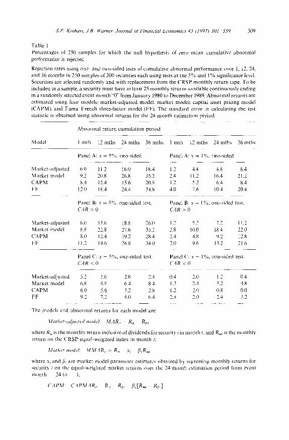
Table 1 reports the percentage of 250 samples for which the null hypothesis of zero abnormal performance is rejected using one- and two-sided tests at 5% and 1% significance levels for each model. Panel A shows that all four models significantly overreject the null hypothesis, and rejection rates increase with the horizon length. For example, the rejection rate using the market model rises from 9.2% over one month to 35.2% over 36 months. The corresponding rejection rates using the FF three-factor model are 12.0% and 34.8%, Generally similar results are obtained at the 1% significance level. The rejection rates for a 36-month horizon range from 8.4% to 20.4%.
Panels B and C report rejection frequencies using one-sided tests. The rejec- tion frequencies in panel B are the percentages of samples for which the models show positive abnormal performance (i.e., reject the null hypothesis when the alternative is that CAR > 0). Panel C shows the percentages of samples for which the models show negative abnormal performance (i.e., reject the null hypothesis when the alternative is that CAR < 0}. Comparison of panels B
S.P. Kothari, J.B. Warner,Journal oJFinancial Economics 43 (1997) 301 339 309
Table 1 Percentages of 250 samples for which the null hypothesis of zero mean cumulative abnormal performance is rejected
Rejection rates using one- and two-sided tests of cumulative abnormal performance over 1, 12, 24, and 36 months in 250 samples of 200 securities each using tests at the 5% and 1% significance level. Securities are selected randomly and with replacement from the CRSP monthly return tape. To be included in a sample, a security must have at least 25 monthly returns available continuously ending in a randomly selected event month "0" from January 1980 to December 1989. Abnormal returns are estimated using four models: market-adjusted model, market model, capital asset pricing model [CAPM), and Fama French three-factor model (FFI. The standard error in calculating the test statistic is obtained using abnormal returns for the 24-month estimation period.
Abnormal return cumulation period
Model 1 mth 12mths 24mths 36mths 1 ruth 12mths 24mths 36mths
Market-adjusted Market model CAPM FF
Panel A: :~ 5%. two-sided Panel A: 7 = 1%. two-sided
6.0 11.2 16.0 18.4 1.2 4.4 4.8 8.4 9.2 20.8 26.8 35.2 2.4 11.2 16.4 21.2 8.4 12.4 15.6 20.8 1.2 5.2 6.4 8.4
12.0 18.4 24.4 34.8 4.0 7.6 10.4 20.4
Panel B: :~ = 5%, one-sided test, CAR > 0
Panel B: z~ = 1%, one-sided test, CAR > 0
Market-adjusted 6.0 13.6 18.8 26.0 1.2 5.2 7.2 11.2 Market model 8.8 22.8 27.6 35.2 2.8 10.0 18.4 22.0 CAPM 8.0 12.4 19.2 28.4 2.4 4.8 9.2 12.8 FF 11.2 19.6 26.8 34.0 2.0 9.6 13.2 21.6
Panel C: :~ = 5%, one-sided test. CAR < 0
Panel C: :~ 1°% one-sided test, CAR < 0
Market-adjusted 5.2 3.6 2.8 2.4 0.4 2.0 1.2 0.4 Market model 6.8 4.8 6.4 8.4 1.2 2.4 3.2 4.8 CAPM 6.0 5.6 3.2 2.8 1.2 2.0 0.8 0.0 FF 9.2 7.2 8.0 6.4 2.8 2.0 2.4 3.2
The models and abnormal returns for each model are:
Market-a~ljusted modeh MARie - Ri~ Rmt
where R. is the monthly return inclusive of dividends for security i in month t. and R.,, is the monthly return on the CRSP equal-weighted index in month t:
M a r k e t model: M M , 4 R . - Ri~ 7 i fliRm~
where 7, and fi~ are market model parameter estimates obtained by regressing monthly returns for security i on the equal-weighted market returns over the 24-month estimation period from event month 24 to 1:
CAPM: C A P M A R , Rir Rfe -- f i ' i[em, e f t 3
310 S.P. Kothari, ,J.B. Warner!Journal o/'Financia/ Economics 43 (1997) 301 339
and C reveals a high degree of a symmet ry in the results. The four models all conclude posi t ive a b n o r m a l per formance over a th ree-year per iod in 26% to 35.2% of the samples at the 5% significance level (panel B), suggest ing posi t ive mean C A R s . In contras t , negat ive a b n o r m a l per formance is observed in only 2.4% to 8.4% of the samples (see panel C). Genera l ly , the rejection rates are close to those expected in the absence of a b n o r m a l performance, a l though some of the models signif icantly overreject the null in panel C. Thus, there can be a tendency to find both posi t ive and negat ive a b n o r m a l per formance too often.
4.2. A b n o r m a l p e r / b r m a n c e m e a s u r e s a n d the i r test s ta t i s t i cs
The test s tat is t ic to assess the stat is t ical significance of mean a b n o r m a l per formance in Table 1 is the ra t io of the (cumulat ive) average a b n o r m a l pe r fo rmance to its es t imated s t anda rd deviat ion. The null will be overrejected if the measured average a b n o r m a l per formance is sys temat ica l ly nonzero or the s t anda rd dev ia t ion used to calcula te the test stat ist ic is too small , o r both. It is also possible that , if the mean and the s t anda rd devia t ion are corre la ted, the test would be misspecified; we do not invest igate this add i t iona l source of misspecifi- cation.
Table 2 presents evidence on mean a b n o r m a l pe r fo rmance (panel A) and the test statist ics (panel B). Since the evidence suggests a n o m a l o u s behavior , we
table I (continued)
wherc /], is from the CAPM regression model [i.e., slope from a regression of (R~, - RI,) on {R,., Ri,) using 24 monthly observations for the estimation period], and Rf, is one-month T-bill return used as a proxy for risk-free return:
FF: F F M A R . = R . - Ri, [~ [R.,t Rr,] - [~2 HML, [~,.~ SMB,
where HML, and SMB, are the Fama-French book-to-market and size factor returns and [1il , fli2, and [3,.3 are estimated by regressing security i's monthly excess returns on the monthly market excess returns, book-to-market, and size factor returns for the 24-month estimation period.
The test statistic for the event month is lillustrated using market-adjusted returns):
M,4R~, ~(MARp,) where M.4Ro, = - ~ M A R , . ]~Tt J ~ l
• I) 6 l I
°"2~/[~Rpr) = f i=~24(!~]/~Ret ,4tyMARe)2 23] , ,du~(,'~IARp) = ~ t=~2, "IARpt ,
and N, is the number of securities that are available in month t.
The test statistic to assess the statistical significance of abnormal performance over a T-month period beginning with the event month "0' is
I 1
CM'4Rt'~ where CM 4R~r = ~ :%IAR~,,. a (MAR~,) .T ~ 2 , ,,
S,P. Kothari, J.B. Warner/Journal (4fFinancial Economics 43 (1997) 301 339 311
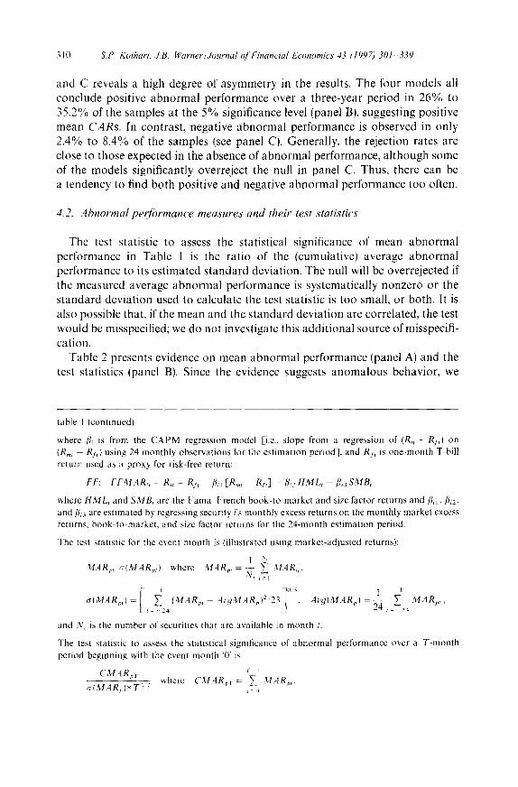
Table 2 Mean abnormal performance measures and test statistics
Mean and standard deviation of cumulative average abnormal returns {CARsj over 1, 12, 24, and 36 months in 250 samples of 200 securities each are reported in panel A. The last three columns report the 25 'h, 50 th, and 75 Ch percentiles of the 36-month CARs. Mean and standard deviation of the test statistics of the CARs are reported in panel B. The last three columns report the 25 th, 50 th, and 75 ~h percentiles of the 36-month test statistics. Securities are selected randomly and with replacement from the CRSP monthly return tape. To be included in a sample, a security must have at least 25 monthly returns available continuously ending in a randomly selected event month "0'" from January 1980 to December 1989. Abnormal returns are estimated using four models: market- adjusted model, market model, capital asset pricing model, and empirical capital asset pricing model. Standard deviation in calculating the test statistic uses the time series of portfolio abnormal returns for the 24-month estimation period.
Panel A: CARs 1%)
CAR I CAR 12 CAR 24 CAR 36 Model Std dvn Std dvn Std dvn Std dvn
Market-adjusted 0.02 1.11 2.09 3.37 0.72 2.75 4.02 5.18
Market model 0.07 1.42 2.62 3.66 0.77 3.31 5.26 7.35
CAPM 0.03 0.95 2.01 3.32 0.74 2.78 4.11 5.37
FF 0.03 0.85 2.28 3.91 0.82 3.13 4.80 6.58
Panel B: Test staustics
Test Test Test Test star I stat 12 star 24 star 36
Model Std dvn Std dvn Std dvn Std dvn
CAR 36 CAR 36 CAR 36 Q 1 Median Q3
-- 0.46 3.43 7.21
l.ll 3.95 8.85
0.53 3.22 7.45
- 0.19 3.83 8.37
Test statistic 36
Q1 Median Q3
Market-adjusted 0.03 0.46 0.61 0.81 - 0.09 0.82 1.66 1.04 1.14 1.17 1.25
Market model 0.11 0.60 0.78 0.90 - 0.27 0.91 2.22 1.16 1.43 1.58 1.79
CAPM 0.05 0.41 0.61 0.82 0.12 0.80 1.79 1.11 1.20 1.24 1,33
H-" 0.05 0.37 0.70 0.99 0.05 0.94 2.03 1.26 1.40 1.50 1.69
The models, abnormal return measures, and test statistics are defined in footnotes to Table 1 and in the text.
further examine mean abnormal performance measures, test statistics, and distributional properties of abnormal returns in Sections 5 and 6.
Panel A reports the mean over 250 simulations of the cumulative average abnormal returns (CARs) over various intervals and its cross-sectional standard
312 S.P. Kothari, J.tt. Warner/Journal o/Financial Economics 43 (1997) 301 339
deviation. Under the null hypothesis, we expect the CARs to be zero. In contrast, they are positive and increase monotonically with the cumulation period. The CAR using the market model averages 0.02% for the event month, but it rises to 1.11% in 12 months, and finally reaches 3.37% in three years. The FF three-factor model yields the highest CAR, 3.91% over a three-year period.
For a perspective on the economic significance of the misspecification, we report the 25 'h and 75 'h percentiles and median of 36-month CARs in the last three columns of Table 2. Median 36-month CARs are close to the means for all four models, which suggests an absence of skewness. The 75 TM percentiles are more than 7%. Thus, in more than one out of four cases, tests would erroneously indicate economically significant abnormal performance.
Panel B of Table 2 reports the mean and cross-sectional standard deviation of the test statistics for the four models over different horizons. Test statistics from well-specified tests should have a zero mean and approximately unit standard deviation, but the observed test statistics have a positive mean and are fat-tailed relative to a unit-normal distribution. The positive mean is expected because mean CARs are positive. We observe a dramatic increase in both means and standard deviations of the test statistics with the cumulation period. The average test statistic in the first month using the market model is 0.11 (cross-sectional standard deviation = 1.04). This increases to 0.90 (cross-sectional standard devi- ation = 1.79) in three years. The high and increasing standard deviation with the horizon suggests that the estimated standard error is too small.
5. Detailed evidence: Mean abnormal performance
This section investigates factors underlying the positive cumulative abnormal return measures in panel A of Table 2. We find that the positive mean abnormal performance is not explained by cumulation bias: tests using buy-and-hold returns, which potentially reduce cumulation bias, are at least as misspecified as those using cumulative abnormal returns (Section 5.1). The cross-sectional distribution of CARs is not positively skewed, so skewness is not the cause of positive mean CARs. For buy-and-hold abnormal returns, however, the cross- sectional distribution of abnormal returns is right-skewed, and the misspecifica- tion of the tests using buy-and-hold abnormal returns appears to be due in part to right-skewness (Section 5.2). There is evidence that the positive mean abnor- mal performance is related to sample-selection biases (Section 5.3) and calendar time-period effects, particularly for the 1980s (Section 5.4).
5.1. Cumulation bias and buv-and-hold returns
Cumulated returns are biased upward and the bias is an increasing function of the proport ionate bid-ask spread of the sample firms (Blume and Stambaugh,
S.P. Kothari, J.B. ffk~rner Journal ~?{ Financial Economics 43 (19971 301 339 313
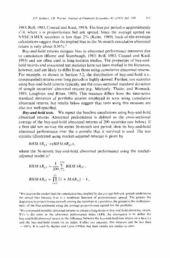
1983; Roll, 1983; Conrad and Kaul, 1993). The bias per period is approximately s2/4, where s is proportionate bid-ask spread. Since the average spread on NYSE/AMEX securities is less than 2% (Keim, 1989), back-of-the-envelope calculations suggest that the implied bias in the 36-month cumulative abnormal return is only about 0.36%. 1
Buy-and-hold returns mitigate bias in abnormal performance measures due to cumulation (Blume and Stambaugh, 1983; Roll, 1983; Conrad and Kaul, 1993) and are often used in long-horizon studies. The properties of buy-and- hold returns and associated test statistics have not been studied in the literature, however, and are likely to differ from those using cumulative abnormal returns. For example, as shown in Section 5.2, the distribution of buy-and-hold (i.e., compounded) returns over long periods is highly skewed. Further, test statistics using buy-and-hold returns typically use the cross-sectional standard deviation of sample securities" abnormal returns (e.g., Michaely, Thaler, and Womack, 1995; Loughran and Ritter, 1995). This measure differs from the time-series standard deviation of portfolio returns employed in tests using cumulative abnormal returns, but results below suggest that tests using this measure are also not well-specified.
Buy-and-hold tests. We repeat the baseline simulations using buy-and-hold abnormal returns. Abnormal performance is defined as the cross-sectional average of the buy-and-hold abnormal returns of 200 securities (see below). If a firm did not survive the entire 36-month test period, then its buy-and-hold abnormal performance over the n months that it survived is used. The test statistic (illustrated using market-adjusted returns) is given by
BHMARp,r/cr(BHMARp-r),
where the 36-month buy-and-hold abnormal performance using the market- adjusted model is 2
1 20o BHMARpl, = ~ ~ BHMARsT,
i= l
35
BHMARi~, = H [1 + MARst] - 1 ,
t -O
1 We caution the reader that the cumulation bias implied by the average bid ask spreads understates the actual bias because bias is a nonlinear function of proportionate spread. The greater the dispersion in proportionate spreads among the securities in a portfolio, the greater is the understate- ment of the bias estimated using the average proportionate spread for the portfolio.
2We compound monthly abnormal returns to obtain a long-horizon buy-and-hold abnormal return. This is the same as the abnormal performance index (API). An alternative is to define the bu1~-and-bold abnormal return as the difference between the buy-and-hold raw return on a security and the buy-and-hold return on an index. Unlike our measure, this measure can be less than
100%. It is used by Barber and Lyon ~1996a), but their results are similar to ours.
314 S.P. Kothari, J.B. Warner~Journal (~/'Financial Economics 43 (1997) 301 339
and the cross-sectional standard deviation of the 36-month mean abnormal returns is
1 V 200 7o.5 (J{BH~?~4ARpT) ~- ~ L i=21(Btt'~/IARiT - B H M A R p T ) 2 J "
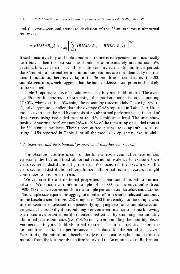
If each security's buy-and-hold abnormal return is independent and identically distributed, then the test statistic should be approximately unit normal. We caution, however, that since all firms do not survive the 36-month test period, the 36-month abnormal returns in our simulations are not identically distrib- uted. In addition, there is overlap in the 36-month test period across the 200 sample securities, which suggests that the independence assumption is also likely to be violated.
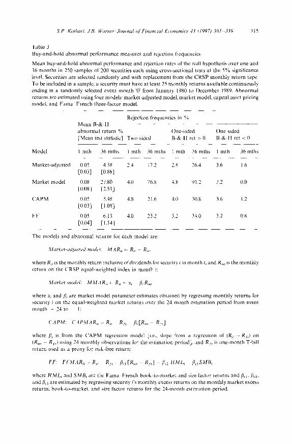
Table 3 reports results of simulations using buy-and-hold returns. The aver- age 36-month abnormal return using the market model is an astounding 27.80%, whereas it is 4 -6% using the remaining three models. These figures are slightly larger, not smaller, than the average CARs reported in Table 2. All four models overreject the null hypothesis of no abnormal performance at the end of three years using two-sided tests at the 5% significance level. The tests show positive abnormal performance 26% to 91% of the time using one-sided tests at the 5% significance level. These rejection frequencies are comparable to those using CARs reported in Table 1 for all the models except the market model.
5.2. Skewness and distributional properties qf long-horizon returns
The observed positive means of the long-horizon cumulative returns and especially the buy-and-hold abnormal returns motivate us to examine their cross-sectional distributional properties. We focus on the skewness of the cross-sectional distribution of long-horizon abnormal returns because it might contribute to misspecified tests.
We examine the distributional properties of one- and 36-month abnormal returns. We obtain a random sample of 50,000 firm event-months from 1980--1989, which corresponds to the sample period in our baseline simulations. This sample size equals the aggregate number of firm-events selected randomly in the baseline simulations (250 samples of 200 firms each), but the sample used in this section is selected independently applying the same sample-selection criteria as before. Fifty thousand long-horizon abnormal returns (one following each security's event month) are calculated either by summing the monthly abnormal return estimates (i.e., CARs) or by compounding the monthly obser- vations (i.e., buy-and-hold abnormal returns). If a firm is delisted before the 36-month test period, its performance is calculated for the period it survived. Substituting the return on a benchmark (e.g., the equal-weighted index) for the months from the last month of a firm's survival till 36 months, as in Barber and
S,P. Kothar i , ,LB. ~i . 'arner,dournal o l ' F i n a n c i a l E c o n o m i c s 43 (1997) 301 339 315
Table 3 Buy-and-hold abnormal performance measures and rejection frequencies
Mean buy-and-hold abnormal performance and rejection rates of the null hypothesis over one and 36 months in 250 samples of 200 securities each using cross-sectional tests at the 5% significance level. Securities are selected randomly and with replacement from the CRSP monthly return tape. To be included in a sample, a security must have at least 25 monthly returns available continuously ending in a randomly selected event month '0' from January 1980 to December 1989. Abnormal returns are estimated using four models: market-adjusted model, market model, capital asset pricing model, and Fama French three-factor model.
Rejection frequencies in % Mean B-&-H- abnormal return % One-sided One sided [Mean test statistic] Two-sided B-&-H ret > 0 B-&-H ret < 0
Model
M arket-adjusted
Market model
CAPM
FF
1 mth 3 6 m t h s I mth 3 6 m t h s 1 mth 3 6 m t h s l mth 3 6 m t h s
0,05 4.38 2.4 17.2 2.8 26,4 3.6 1.6 [0,03] [0.86]
0.08 27.80 4.0 76.8 4.8 91.2 3.2 0.0 [0.08] [2.51]
0.05 5.48 4.8 21.6 4.0 30.8 3.6 1.2 [0.03] [J.os]
0.05 6.13 4.0 23.2 3.2 34.0 3.2 0.8 [0.O4] [ 1.14]
The models and abnormal returns for each model are:
M a r k e t - a d j u s t e d model: M A R . = Re, - R . .
where R . is the monthly return inclusive of dividends for security i in month < and Rm, is the monthly return on the CRSP equal-weighted index in month t:
M a r k e t model: M M A R i , Ri, - :q - fi, Rm,
where :~ and fi~ are market model parameter estimates obtained by regressing monthly returns for security i on the equal-weighted market returns over the 24-month estimation period from event month - 2 4 t o 1:
CAP.~.I: C A P M A R i , = R . -- RI~ f i i [R , , , - R~,]
where fi, is from the CAPIM regression model [i.e.. slope from a regression of (Ri, - Rr , ) o n
(R,,, Rr,) using 24 monthly' observations for the estimation period], and RI, is one-month T-bill return used as a proxy, for risk-free return:
FF: F F M A R ~ , = R . - R~, - f i~ [R~ , R r , ] - fi~2 H M L , - f i ~ S M B ,
where H M L , and S M B ~ are the Fama French book-to-market and size factor returns and fii~. fl~2, and fl~3 are estimated by regressing security i's monthly excess returns on the monthly market excess returns, book-to-market, and size factor returns for the 24-month estimation period.
316 S.P. Kolhari, ZB. Warner/Journal (2,/'Financial Economics 43 (1997) 301 339
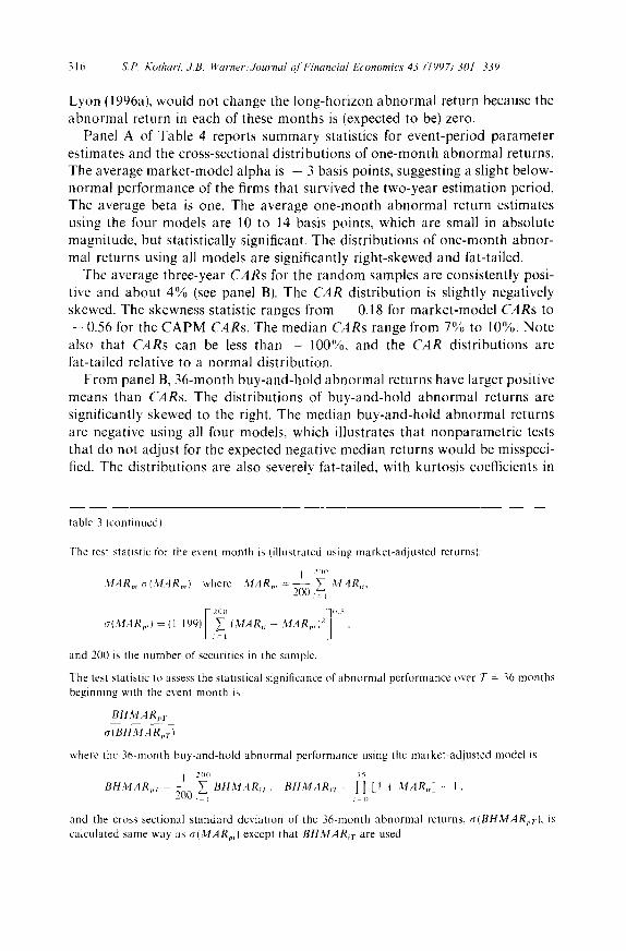
Lyon (1996a1, would not change the long-hor izon a b n o r m a l re turn because the a b n o r m a l re turn in each of these mon ths is (expected to be) zero.
Panel A of Table 4 repor ts s u m m a r y statist ics for event -per iod p a r a m e t e r es t imates and the cross-sect ional d i s t r ibu t ions of o n e - m o n t h a b n o r m a l returns. The average m a r k e t - m o d e l a lpha is - 3 basis points , suggesting a slight below- normal per formance of the firms that survived the two-year es t imat ion period. The average beta is one. The average one -mon th a b n o r m a l re turn es t imates using the four models are 10 to 14 basis points, which are small in abso lu te magni tude , but s tat is t ical ly significant. The d i s t r ibu t ions of o n e - m o n t h abnor - mal returns using all models are signif icantly r ight -skewed and fat-tailed.
The average three-year C A R s for the r a n d o m samples are consis tent ly posi- tive and abou t 4 % (see panel B). The C A R dis t r ibu t ion is sl ightly negat ively skewed. The skewness stat ist ic ranges from - 0.18 for m a r k e t - m o d e l C A R s to - 0.56 for the C A P M C A R s . The median C A R s range from 7% to 10%. Note
also that C A R s can be less than - 100%, and the C A R dis t r ibu t ions are fat- tai led relat ive to a no rma l d is t r ibut ion.
F r o m panel B, 36-month buy -and -ho ld a b n o r m a l re turns have larger posi t ive means than CARs . The d is t r ibu t ions of buy -and -ho ld a b n o r m a l returns are significantly skewed to the right. The median buy -a nd -ho ld a b n o r m a l re turns are negative using all four models, which i l lustrates tha t nonpa ra me t r i c tests that do not adjus t for the expected negative median re turns would be misspeci- fled. The d i s t r ibu t ions are also severely fat- tai led, with kur tos is coefficients in
table 3 (continued)
The test statistic for the event month is (illustrated using market-adjusted returnsl:
] 2o0 :XlARp, a(.XtAR.,,I where M A R . , = - - }Z M A R . .
200 i% 200 "]05
~(MARp,} = ,1 199) I ~ l I M A R , r - M A R , , ) 2 .
and 200 is the number of securities in the sample,
The test statistic to assess the statistical significance of abnormal performance over T = 36 months beginning with the event month is
BHMARv~
a(BHMARpr)
where the 36-month buy-and-hold abnormal performance using the market-adjusted model is
1 2Ira i~ BHMAR~ = - - V_. BHM.dRil. BHMAR,-t -- [1 + MARir ] -- 1.
' 200 ~ = ~ , = (,
and the cross-sectional standard deviation of the 36-month abnormal returns, o{BHMARpr), is calculated same way as a(MARp,) except that BHMAR~7 are used.
S.P. Kothari, J.B. Warner~Journal o/Financial Economics 43 (1997) 301 339 317
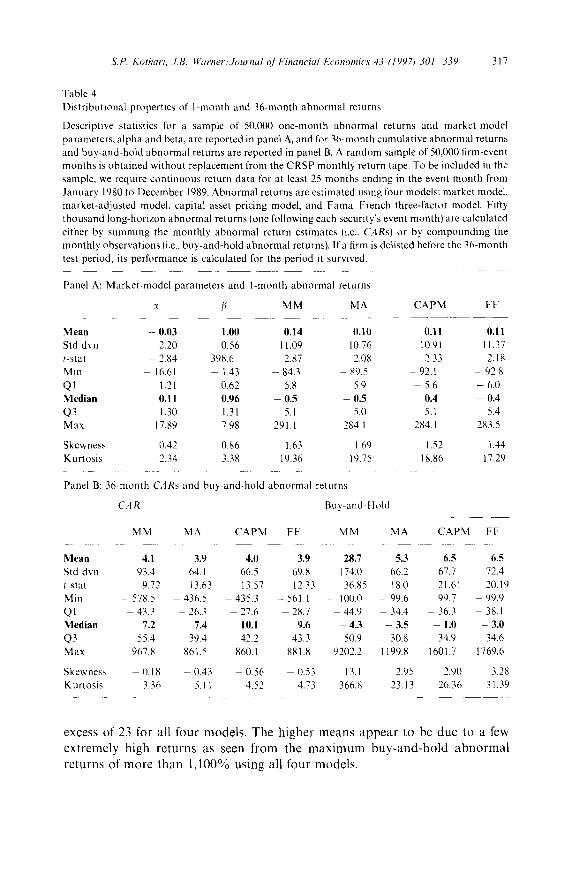
Table 4 Distributional properties of 1-month and 36-month abnormal returns
Descriptive statistics for a sample of 50,000 one-month abnormal returns and market-model parameters, alpha and beta, are reported in panel A, and for 36-nronth cumulative abnormal returns and buy-and-hold abnormal returns are reported in panel B. A random sample of 50,000 firm-event months is obtained without replacement from the CRSP monthly return tape. To be included in the sample, we require continuous return data for at least 25 months ending in the event month from January 1980 to December 1989. Abnormal returns are estimated using four models: market model. market-adjusted model, capital asset pricing model, and Fama French three-factor model. Fifty thousand long-horizon abnormal returns (one following each security's event month) are calculated either by summing the monthly abnormal return estimates {i.e.. CARs} or by compounding the monthly observations (i.e., buy-and-hold abnormal returns). Ira firm is delisted before the 36-month test period, its performance is calculated for the period it survived.
Panel A: Market-model parameters and l-month abnormal returns
:~ fi MM MA CAPM FF
M e a n - 0.03 1.00
Std dvn 2.20 0.56 t-star 2.84 398.6 Min 16.61 - 1.43 QI 1.21 0.62 M e d i a n 0.11 0.96
Q3 1.30 1.31 Max 17.89
Skewness 0.42 Kurtosis 2.34
Panel B: 36-month CARs
CAR
MM MA
M e a n 4.1 3.9
Std dvn 93.4 64 1 t-stat 9.72 13.63 Min - 578.5 436.5 Q1 43.3 26.3 M e d i a n 7.2 7.4
Q3 55.4 39.4 Max 967.8 861.5
Skewness - 0.18 - 0.43 Kurtosis 3.36 5.11
7.98
0.86 3.38
0.14 0.10 0.11 0.11
11.09 10.76 10.91 11.37 2.87 2.08 2.33 2.18
- 84.3 -- 89.5 92.1 - 92.8 5.8 - 5.9 5.6 -- 6.0 0.5 0.5 - 0.4 0.4
5.1 5.0 5.1 5.4 291.1 284.1 284.1 283.5
1.63 1.69 1.52 1.44 19.36 19.75 18.86 17.29
and buy-and-hold abnormal returns
Buy-and-Hold
CAPM FF MM MA CAPM FF
4.0 3.9 28.7 5.3 6.5 6.5
66.5 69.8 174.0 66.2 67.7 72.4 13,57 12.33 36.85 18.0 21.61 20.19
435,3 -- 561.1 -- 100.0 - 99.6 99.7 - 99.9 27.6 28.7 - 44.9 34.4 36.3 - 38.1 I0.1 9.6 - 4.3 -- 3.5 1.0 - 3.0
42.2 43.3 5t/.9 30.8 34.9 34.6 860.1 881.8 9202.2 1 1 9 9 . 8 1 6 0 1 . 7 1769.6
0.56 0.53 13.1 2.95 2.90 3.28 4.52 4.73 366.8 23.13 26.36 31.39
e x c e s s o f 23 fo r all f o u r m o d e l s . T h e h i g h e r m e a n s a p p e a r to be d u e to a few
e x t r e m e l y h i g h r e t u r n s as s een f r o m t h e m a x i m u m b u y - a n d - h o l d a b n o r m a l
r e t u r n s o f m o r e t h a n 1 , 1 0 0 % u s i n g all f o u r m o d e l s .
318 sP. Kothari, ,LB. Warner/Journal q/kTnancial Economics 43 (1997) 301-339
The mean buy-and-hold abnormal return using the market model is very large, 28.7%. The estimated constant term, alpha, of the market model reflects ex post average abnormal performance and estimation error. Neither is expected to persist into the future, but the estimated test-period abnormal performance contains the compounded value of alpha. The resulting buy-and-hold abnormal performance is right-skewed with a large mean. 3
5.3. Sample-select ion bias and surt'ival
We include firms even when they do not survive the entire 36-month test period, but there nevertheless are selection biases in our samples. The "randomly' selected samples of 200 firms exclude firms with returns unavailable for the entire 24-month estimation period, These firms either were listed during the estimation period or the test period, or were delisted during the estimation period. Thus, the firms that were listed on the New York and American stock exchanges following initial public offerings or after moving from other ex- changes are not included in random samples. Research suggests that these firms' post-listing performance has been systematically negative in the 1970s and 1980s (Loughran and Ritter, 1995), although Bray and Gompers (1995) question the economic significance of this conclusion. If post-listing underperformance is not due to test misspecification, a systematic exclusion of these firms from our samples will impart an opposite positive bias to the average C A R for the included firms.
Another characteristic of the two sets of firms excluded from our samples is that they are likely to be relatively small market-capitalization stocks. Small firms underperformed relative to the market (or the CAPM benchmark) in the 1980s (see, for example, Fama and French, 1995, p. 141). Systematic exclusion of the small firms from our ' random' samples would bias upwards the estimated abnormal performance using some of the models.
We study securities' average test-period returns conditional on various inter- vals of estimation-period survival. We begin with all firms with nonmissing return data on the CRSP monthly return tape for the month of January 1980 without requiring any past data (i.e., zero survival period). For this sample, we calculate one-month, one-year, two-year, and three-year test-period cumulative returns beginning in January 1980. If a firm did not survive the entire test period, its returns for the period of its survival are included. We then move the window
3The observed properties of buy-and-hold abnormal returns motivated us to consider continuously compounded returns as a statistical means of "correcting' the properties. The mean three-year continuously compounded market-adjusted return is 15% and the median is -3 .5%. The distribution is significantly negatively skewed and fat tailed. Therefore. tests using continuously compounded returns are unlikely to be well-specified.
S.P. Kothari, J.B. Warner/Journal ol'Financial Economics 43 (1997) 30l 339 319
forward one month at a time until December 1990. The grand means of the one-month and the one-, two-, and three-year cumulative return observations are reported in the first row of panel A of Table 5. The number of observations in each sample is 317,709.
We then repeat the above experiment with only firms having at least 12 months of continuous prior return data. The sample size declines to 296,341. This procedure is repeated for two-, three-, and four-years of prior survival. The average returns conditional on these survival intervals are reported in rows 2 through 5 in panel A of Table 5. Note that both no-data requirement and four-year-data requirement sample periods begin each month starting from January 1980 till December 1990. Thus, there is no difference in the calendar
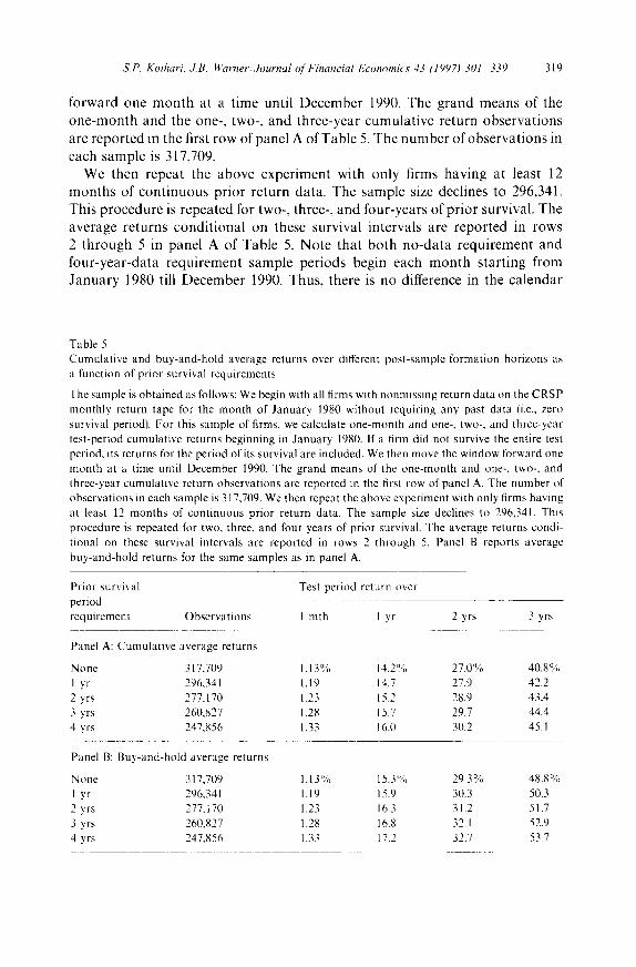
Table 5 Cumulative and buy-and-hold average returns over different post-sample formation horizons as a function of prior survival requirements
The sample is obtained as follows: We begin with all firms with nonmissing return data on the CRSP monthly return tape for the month of January 1980 without requiring any past data (i.e., zero survival period). For this sample of firms, we calculate one-month and one-, two-, and three-year test-period cumulative returns beginning in January 1980. If a firm did not survive the entire test period, its returns for the period of its survival are included. We then move the window forward one month at a time until December 1990. The grand means of the one-month and one-, two-, and three-year cumulative return observations are reported in the first row of panel A. The number of observations in each sample is 317,709. We then repeat the above experiment with only firms having at least 12 months of continuous prior return data. The sample size declines to 296341. This procedure is repeated for two, three, and four years of prior survival. The average returns condi- tional on these survival intervals are reported in rows 2 through 5. Panel B reports average buy-and-hold returns for the same samples as in panel A.
Prior survival Test period return over period requirement Observations I mth 1 yr 2 yrs 3 yrs
Panel A: Cumulative average returns
None 317,709 1.13 % 14.2 % 27.0% 40.8 % I yr 296,341 1.19 14.7 27.9 42.2 2 yrs 277,170 1.23 15.2 28.9 43.4 3 yrs 260,827 1.28 15.7 29.7 44.4 4 yrs 247,856 1.33 16.0 30.2 45.1
Panel B: Buy-and-hold average returns
N one 317,709 1.13 % 15.3 % 29.3 % 48.8 % 1 yr 296,341 1.19 15.9 30.3 50.3 2 yrs 277,170 1.23 16.3 31.2 51.7 3 yrs 260,827 1.28 16.8 32.1 52.9 4 yrs 247,856 1.33 17.2 32.7 53.7
320 S.P. Kothari. J.B. Warner:Journal ()['Financial Economics 43 (1997) 301 339
periods over which average returns, conditional on various lengths of data availability periods, are calculated.
The results in Table 5 strongly suggest that conditioning a sample on prior return data availability is associated with higher future mean returns. As the prior data availability requirement is increased from zero to four years, the average future three-year return increases from 40.8% to 45.1%. In panel B of Table 5, similar results apply with buy-and-hold average returns. For example, the average three-year return conditional on no data requirement is 48.8%. This increases to 53.7% with a four-year data requirement.
One implication of the results in Table 5 is that average returns for a random sample of firms meeting a past-data requirement will exceed those for random samples with no past-data requirement. Thus, market-adjusted returns will be systematically positive. The difference between the cumulative average three- year return for the sample with a two-year data requirement and the sample without any data requirement is 2.6%. This is comparable to the observed mean market-adjusted three-year CARs reported in Tables 2 4. Thus, sample-selec- tion bias is an important determinant of the misspecification we document. This conclusion is unchanged if market-adjusted returns are used directly. For example, we obtain a mean three-year market-adjusted return of 3.3% for the sample with a two-year prior-data requirement.
The increase in average returns as a function of a seemingly innocuous data availability requirement is quite unexpected, but the results for market-adjusted returns are also consistent with independent work by Barber and Lyon (1996a, Table 51. They report a three-year mean CAR of 3.46% using the equal-weighted market-adjusted model. This increases to 6.27% by the end of five years. While Barber and Lyon do not require any past return data, their criteria for a sample firm's inclusion impose other past-data requirements. In particular, they require that fnancial data be available on the Compustat tapes to enable them to calculate the book-to-market ratio (see also Kothari, Shanken, and Sloan, 1995, for a discussion of biases introduced by the Compustat data availability require- ment).
Turning attention to mean three-year buy-and-hold abnormal returns, the mean reported in our Table 4 is much larger than the 0.10% average buy-and-hold abnormal return reported by Barber and Lyon (1996a, Table 7). The difference in their mean and that reported in Table 4 in this study could be because they include NASDAQ stocks (see Barber and Lyon, 1996b, for a detailed analysis).
Although market-adjusted returns provide a dramatic illustration, abnormal returns that are systematically nonzero because of pre-event survival-related biases would not be surprising for other benchmarks. Although we cannot examine our other benchmarks because they require estimation-period para- meter estimates, we discuss matched portfolio tests in Section 7.2. Survivor biases are a potential issue with these procedures if the survival criteria for
S,P. Kothari, J.B. f~'arner,Journal (~/'Financial Economics 43 (1997j 301 339 321
inclusion in a sample differ from the survival criteria for firms in a matched portfolio. For example, Loughran and Ritter (1995) compare initial public offering stocks" performance against a portfolio that had survived at least five years. Such pre-event survivor biases are one possible explanation for the misspecification of matched portfolio tests.
5.4. Calendar time period and other effects
To examine whether our baseline simulation results are sensitive to calendar period (e.g., 1980s) effects, we repeat the simulations for different time periods, including 1965-89, 1928--1962, and 1928--89. To save space, results of these and other sensitivity checks in this section are not shown in the tables. Generally, most models appear misspecified over the different periods. The 36-month average CARs are roughly 2% and rejection frequencies are somewhat lower in other periods, particularly pre-1962, than in the 1980s.
The slightly better specification of the tests in the pre-1962 period, which use only NYSE stocks, motivated us to examine whether the tests in the post-1962 period are misspecified because AMEX stocks are included in the simulation samples. Results of simulations using only NYSE stocks in the 1965 89 period are similar to those for NYSE/AMEX stocks for all the models except the market-adjusted model. Since the average beta of the random samples of NYSE stocks, estimated using the CRSP equal-weighted NYSE/AMEX index, is 0.88, market-adjusted returns are on average negative (e.g., 36-month average CAR is - 0.82%). Therefore, the market-adjusted model concludes negative abnormal
performance excessively. We also repeat simulations separately for other decades, restricting the event
month to the 1950s, 1960s, or 1970s. All four models exhibit excessive rejection rates in the 1970s. The market-adjusted model is quite well-specified in the 1950s and 1960s, while the market model exhibits excessive rejection rates in all the ten-year periods and the performance of CAPM is mixed.
We also investigate whether risk nonstationarity explains our baseline results. In order for beta increases to explain the observed abnormal performance of 3 4% in 36 months, assuming a risk premium of 8% per annum, the CAPM beta must increase by 0.13 to 0.17 from the estimation period to the test period. A priori, this seems unlikely for portfolios consisting of 200 randomly selected securities. Indeed. we find average beta changes of only 0.02 or less.
6. Detailed evidence: The estimated standard deviation
The reader will recall that the test statistics are fat-tailed relative to a unit- normal distribution and that this behavior worsens with horizon length. There are three reasons why the standard deviations from the estimation-period

322 S.P. Kothari, J.B. Warner.,Journal t f Financial Economics 43 (1997) 3Ol 339
returns, which are used to calculate the test statistics, are too small. The most important is that there are survival-related variance shifts (Section 6.1). In addition, firms that drop out during the test period affect the estimated standard deviation (Section 6.2), and test-period prediction errors are more variable than fitted residuals from the estimation period (Section 6.3).
6.1. Survival and individual security variance shi[is
The baseline simulations impose a 24-month pre-event data availability requirement, and these returns are used to estimate the standard deviation. (As discussed in Section 6.3, the misspecification of the test is not sensitive to the length of the estimation period.) Detailed empirical analysis reveals, however, that for the firms that survive a given period, ex post return variance (i.e., estimation-period variance) is considerably lower than the variance uncondi- tional on further survival (i.e., test-period variance). The measured variance of the estimation-period returns thus underestimates the test-period variance. This bias likely arises because a firm is included in our sample only if it survived the previous two years. The ex post variance therefore does not reflect the typically high variability of failing firms, which would be reflected in an unconditional estimate of return variance.
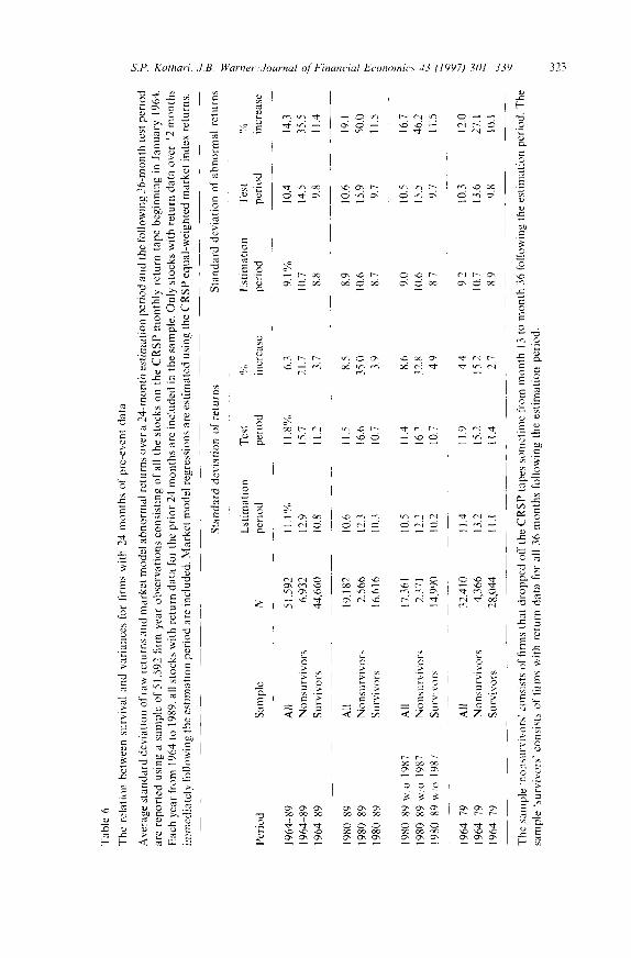
Table 6 reports the average standard deviation of monthly returns and monthly abnormal returns (market model residuals or prediction errors) esti- mated for a 24-month estimation period and 36-month test period for all the stocks on the CRSP monthly return tape beginning in 1964. Each year all stocks with return data for the prior 24 months are included in the sample. Since a time series of returns is needed to estimate standard deviation over the test period, we only include stocks with return data over 12 months immediately following the estimation period. That is, there is a modest data requirement beyond the estimation period.
There are 51,592 firm-year observations that meet the above criteria. Estima- tion-period abnormal returns are defined as residuals from a market-model regression and test-period abnormal returns are prediction errors. The average standard deviation of estimation-period monthly returns is 11.1%, compared to 11.8% in the test period, an increase of 6.3%. The corresponding increase in the standard deviation of abnormal returns is from 9.1% to 10.4%, a jump of 14.3%.
The results for subsamples formed on the basis of whether or not the firm survived the three-year test period reveal that nonsurvivors' return variability in the test period is substantially higher than in the estimation period. For example, during the 1980s, the nonsurvivors' standard deviation of returns (abnormal returns) rose by 35% (50%). Out of a total of 19,182 firm-year observations in the 1980s, 2,566 or about 13% were delisted during years 2 and 3 after the estimation period. The survivors' standard deviation of returns also
S.P. KotharL J.B. Warner,Journal o/ 'Financial Ecom>mics 43 (1997) 301 339 323
Y:
.= E
eo
E
E
t .
g
"r-
¢)
2
"~ -5
~- <
m ",7,
.'7~. "~ ~.~ .g=8
e-
~ °
~ = [g ,..2 ~ ' ' ' "
. ~ ~
g . ~
"-o ca
E ..,: ~ . =
~ . - ~ . .
t.% i--- f--4 ks%, ~ r-~
G
r- o l l
:.< ~ ' -: - - ; o 6 , r ; , <
c~
¢"1 ¢ 'q
~ ~ ~ ~ " ~'~I t ~'~
od c-i + ~: m; ,'-i
c c
~ z g ~
~2
©
g~ ~ z ~
Q
0
=_ G
E £-8 ¢.~, C,
.E 2:
=-£
..g2
E ' ~ ,
E
324 S.P. Kolhari, ,I,13. Warner/Journal {?/'Financial Economics 43 (1997) 301 339
rises, but the increase is a modest 3.9%. The results for various subperiods reported in Table 5 are similar.
Given the variance shift between estimation and test period, there are several ways of addressing the bias in estimated standard deviation of abnormal returns. Use of a standard deviation estimated from test-period or the post-test- period returns might mitigate the overrejection of the null hypothesis of zero abnormal performance. Test-period standard deviations can be estimated cross-sectionally or using time series data. The simulation results reported earlier using buy-and-hold returns employed cross-sectional test-period stan- dard deviations, but did not produce any significant reduction in the overrejec- tion rates. Results using standard deviations estimated from test-period and post-test-period time series of returns are presented later in the paper. None of the procedures alters the degree of misspecification of the tests and each of the procedures suffers from somewhat different theoretical weaknesses.
6.2. Drop-out.firms and variance estimation
Since some of the firms from the initial samples of 200 firms do not survive the 36-month test period, the sample size declines throughout this period. Variabil- ity of portfolio returns is a decreasing function of sample size. This is another reason the standard deviation calculated using the estimation-period portfolio return data understates the standard deviation of the test-period returns. The numbers of survivors and nonsurvivors reported in Table 6 suggest that the sample size is reduced by approximately 15% by the end of the three-year test period. The implied standard deviation of the mean in the test period's last month would be approximately 8.5% [ = (200/170) o.5 - 1] higher than that during the estimation period due solely to a sample size decline. Smaller increases are expected in the early months of the test period.
While the estimation-period standard deviation is a downward-biased esti- mate in the tests because of drop-out firms, note that in the tests of buy-and-hold abnormal performance, returns of all firms, including drop-out firms, were included in calculating the cross-sectional standard deviation (see Table 3). These tests were misspecified too. Therefore, it is unlikely that drop-out firms would fully explain the misspecification of the long-horizon tests.
Use of the standard deviation estimated from the time series of test-period abnormal returns can, in part, correct the problem arising from an increase in return variability due to drop-out firms. Note, however, that the true standard deviation of the portfolio changes during the test period because the sample size is changing over the test period due to drop outs. Table 7 reports rejection frequencies in the event month and over three years based on tests that employ the time series of test-period portfolio abnormal returns to calculate the stan- dard deviation. The standard deviation calculation is exactly as in Eqs. (7)49), except that the 24 monthly estimation-period observations are replaced by the
S.P. Kothari. J.B. Warner Journal o/'Financial Economics 43 (1997) 301 339 325
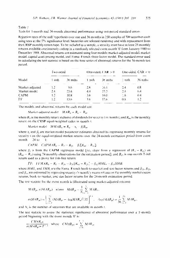
Table 7 Tests for 1-month and 36-month abnormal performance using test-period standard errors
Rejection rates of the null hypothesis over one and 36 months in 250 samples of 200 securities each using tests at the 5% significance level. Securities are selected randomly and with replacement from the CRSP monthly return tape. To be included in a sample, a security must have at least 25 monthly returns available continuously ending in a randomly selected event month '0' from January 1980 to December 1989. Abnormal returns are estimated using four models: markebadjusted model, market model, capital asset pricing model, and FFama French three-factor model. The standard error used in calculating the test statistic is based on the time series of abnormal returns for the 36-month test period.
Two-sided One-sided, CAR > 0 One-sided, CAR < 0
Model 1 mth 36 mths 1 ruth 36 mths 1 mth 36 mths
Market-adjusted 1.2 9.6 2.8 16.4 2.4 0.8 Market model 2.4 23.6 4.4 27.2 2.8 6.4 CAPM 1.2 10.8 3.6 16.0 1.6 0.4 FI r 1.2 13.6 3.6 17.6 0.8 1.2
The models and abnormal returns for each model are:
Mclrket-adjusted model: MARie = R . - R . .
where R. is the monthly return inclusive of dividends for security i in month t. and R,., is the monthly return on the CRSP equal-weighted index in month t:
Market model: M M A R , = Ri, - :q [~iRm,
where x, and/~ are market model parameter estimates obtained by regressing monthly returns for security i on the equal-weighted market returns over the 24-month estimation period from event month - 2 4 t o - 1:
CAPM: C A P M A R i , = R , - Rr, [~i[R,m - - Rt~ ]
where [$i is from the CAPM regression model [i.e., slope from a regression of (Rf, - R/,) on (Rm, - Rft) using 24 monthly observations for the estimation period], and Rr, is one-month T-bill return used as a proxy for risk-free return:
FF: FFMAR~, - R , R D - - [ 1 i l JR,,, - R2~ ] - []~2HML, [4,3SMBt
where H M L , and SMB, are the Fama French book-to-market and size factor returns and [~,1, [~,_. and [],3 are estimated by regressing security i's monthly excess returns on the monthly market excess returns, book-to-market, and size factor returns for the 24-month estimation period.
The test statistic for the event month is (illustrated using market-adjusted returns):
1 "~ M.4Re~ ~r{MAR.,) where MARt, ̀ = ~ ~ M A R . .
35 ] (15 I~U 35 aIMAR.~) V IM,4Rpt -- - "4vgMARp 12:35 ' '4v~t(MARe) -- T2 ~ MARe"
Lr= ~ t=(I and N, is the number of securities that are available in month t.
The test statistic to assess the statistical significance of abnormal performance over a T-month period beginning with the event month "0" is:
]" 1 CMARpl where CMARpr = ~ MARp,
(~(MARp)* T 1 2 ~=o
326 S.P. Kotkari, ZB. Warner:Journal qI bTnancial Economics 43 (1997) 301-339
36 from the test period. The null hypothesis of no abnormal performance in the event month is underrejected by all four models using the two-sided test at the 5% significance level. Since the test-period standard deviation reflects the effect of a decline in sample size with the length of the test-period and because none of the 200 sample firms is missing in the event month, the test-period standard deviation is too high for the event month. This results in rejecting the null too infrequently.
All four models exhibit excessive rejection frequencies over three years. The market model performs the worst, whereas the CAPM and market-adjusted models exhibit comparable performance. All four models' rejection frequencies are lower than those using the estimation-period standard deviation. Thus, the use of test-period standard deviation mitigates, but does not eliminate, the incidence of overrejection.
Table 7 also reveals that the four models' rejection rates are not symmetric. The tests conclude positive abnormal performance in three years too often, but negative performance is concluded too infrequently. This is due in part to the positive mean CARs that rise with the cumulation period for reasons discussed earlier.
6.3. Prediction error variability
Prediction errors are more variable than fitted residuals from a regression (e.g., Maddala, 1988, p. 52). The fewer the number of estimation-period observa- tions, the greater the difference between the variability of residuals and predic- tion errors: the higher the volatility of the market return in the test period compared to the estimation period, the higher the prediction error variability. This naturally contributes to excessive rejection frequencies, but does not entirely account for the excessive rejection frequencies observed earlier for at least two reasons. First, the market-adjusted model, which does not entail parameter estimation, also rejects the null hypothesis too often. Second, the observed rejection rates are too high to be explained entirely by the understate- ment of prediction errors' variability. We also note that the results in Table 7 reveal that using test-period standard error (which is free from the understate- ment problem) also yields excessive rejection.
Other things equal, a longer estimation period yields more precise parameter estimates for the return-generating process and a more accurate estimate of the variability in abnormal returns. We therefore repeat the simulations using a 48-month estimation period. This also imposes a more stringent data avail- ability requirement and thus survival-related biases discussed in Section 6.1 could be more serious than in the baseline simulations.
Rejection frequencies based on one- and two-sided tests at the 5% significance level and using estimation- and test-period standard deviations are reported in Table 8. The time period is restricted to the 1980s. The null hypothesis of no
S.P. Kothari. J B . Warner~Journal qf 'Financial Economics 43 (1997) 301 339 327
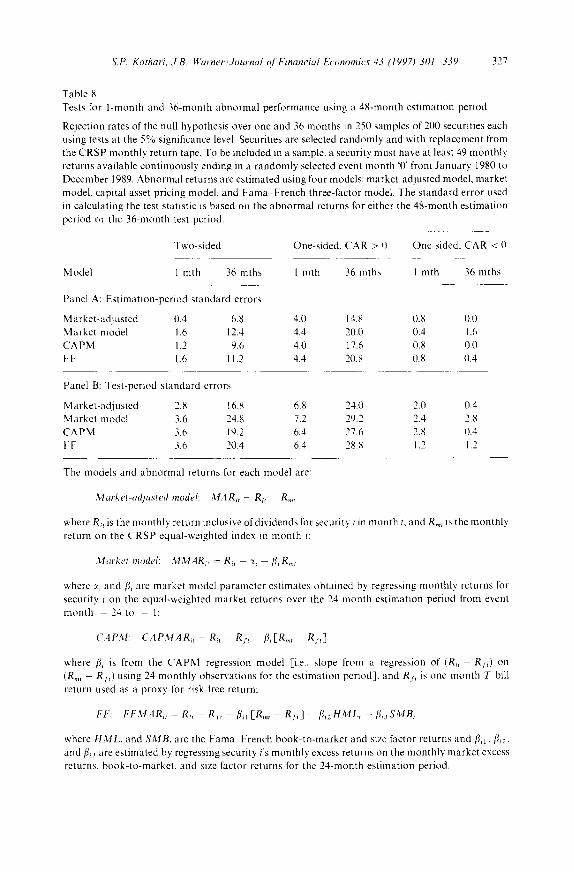
Table 8 Tests for l-month and 36-month abnormal performance using a 48-month estimation period
Rejection rates of the null hypothesis over one and 36 months in 250 samples of 200 securities each using tests at the 5% significance level. Securities are selected randomly and with replacement from the CRSP monthly return tape. To be included in a sample, a security must have at least 49 monthly returns available continuously ending in a randomly selected event month ~0' from January 1980 to December 1989. Abnormal returns are estimated using four models: market-adjusted model, market model, capital asset pricing model, and Fama French three-factor model. The standard error used in calculating the test statistic is based on the abnormal returns for either the 48-month estimation period or the 36-month test period.
Two-sided One-sided. CAR > 0 One-sided, CAR < 0
Model 1 mth 36 mths I mth 36 mths 1 mth 36 mths
Panel A: Estimation-period standard errors
Market-adjusted 0.4 6.8 4.0 14.8 0.8 0.0 Market model 1.6 12.4 4.4 20.0 0.4 1.6 CAPM 1.2 9.6 4.0 17.6 0.8 0.0 FF 1.6 11.2 4.4 20.8 0.8 0.4
Panel B: Test-period standard errors
M arket-adjusted 2.8 16.8 6.8 24.0 2.0 0.4 Market model 3.6 24.8 7.2 29.2 2.4 2.8 CAPM 3.6 19.2 6.4 27.6 2.8 0.4 F F 3.6 20.4 6.4 28.8 1.2 1.2
The models and abnormal returns for each model are:
Market-adjusted model: M A R , - Ri, R,,,t
where R~, is the monthly return inclusive of dividends for security i in month t, and R~ is the monthly return on the CRSP equal-weighted index in month t:
Market model: 3.tMARi~ - Ri, - ~i f l iR t ,
where :~ and fi~ are market model parameter estimates obtained by regressing monthly returns for security i on the equal-weighted market returns over the 24-month estimation period from event month 24 to - 1:
C A P M : C A P M A R i t = R e , - R r' fli[R,.,, Rt ,]
where l], is from the CAPM regression model [i.e.. slope from a regression of (Ri, Rr~) on (R,,,, Rr,) using 24 monthly observations for the estimation period], and Rr, is one-month T-bill return used as a proxy for risk-free return:
FF: F F M A R . - R~, Rr, fl,~ [R.,, - Rr, ] - f i~zHML, - [4~.sSMB,
where H M L , and S M B , are the Fama French book-to-market and size factor returns and /Jil, [~i2" and fl~3 are estimated by regressing security i's monthly excess returns on the monthly market excess returns, book-to-market, and size factor returns for the 24-month estimation period.
328 S.P. Kothari, J.B. Warner/Journal ol'Financial Economics 43 (1997j 301 339
effect is rejected too infrequently in the event month, but it is rejected too frequently by the end of 36 months by all models except the market-adjusted model. However, in one-sided tests, all four models indicate positive abnormal performance excessively (14.8% to 20.8%). In contrast , negative abnormal performance in the event mon th as well as at the end of 36 months is indicated too infrequently by all four models. The rejection rates at the end of 36 months are very high for all four models using test-period s tandard errors (16.8% to 24.8%). Overall, the results reveal that the use of a longer estimation period does not alter the inferences from the baseline simulations.
7. Robustness checks
This section summarizes additional robustness checks. Long-hor izon tests using n o n r a n d o m samples are misspecified and generate both positive and negative estimated long-horizon abnormal performance (Section 7.1). Tests using returns on portfolios matched by size and book- to -marke t do not alter the overall conclusion of misspecification (Section 7.2). Finally, our general results on misspecification are also robust to many other test procedure variations (Section 7.3).
7.1. Nonrandom samples
N o n r a n d o m samples can have firm characteristics that are correlated with the determinants of firms' expected rates of return. This can result in biased abnormal returns if the correct benchmark is not used. Since previous research indicates that the book- to-marke t ratio and firm size are correlated with firms'
table 8 Icontinuedi
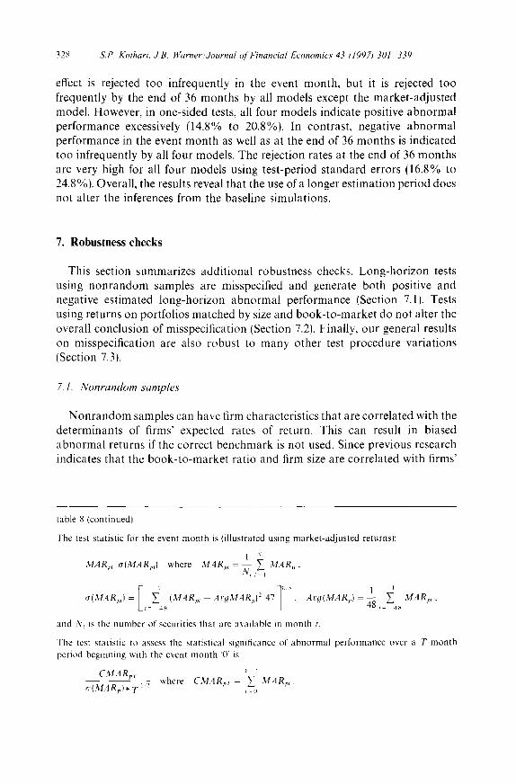
The test statistic for the event month is (illustrated using market-adjusted returns): | ' ,
MAR,,, a(MARp,) where MARp, = . ~ i~1 M.4Ri,,
= .4rgMARp )2'47 o.~ 1
and N, is the number of securities that are available in month t.
The test statistic to assess the statistical significance of abnormal performance over a T-month period beginning with the event month '0' is
C M ,4 R p i ~ ~(MARp)* T 1.2 where CMARp.: = :=ll~ MAR:,t .
S.P. Kothari, J.B. Warner/Journal Of Financial Economics 43 (1997) 301 339 329
average returns, we perform simulations using samples consisting of either high or low book-to-market firms and small- or large-sized firms.
Low (high) book-to-market samples have securities with a book-to-market ratio of 0.8 or less (one or more} at the beginning of the year of the randomly selected event month. Approximately 40% of the population of stocks have book-to-market ratios below 0.8 or above one. Because the total number of securities available for obtaining low or high book-to-market samples is con- siderably smaller than that in the baseline simulations, we allow the event month to be anywhere between January 1970 and December 1989, instead of only in the 1980s.
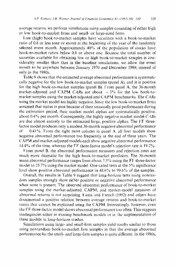
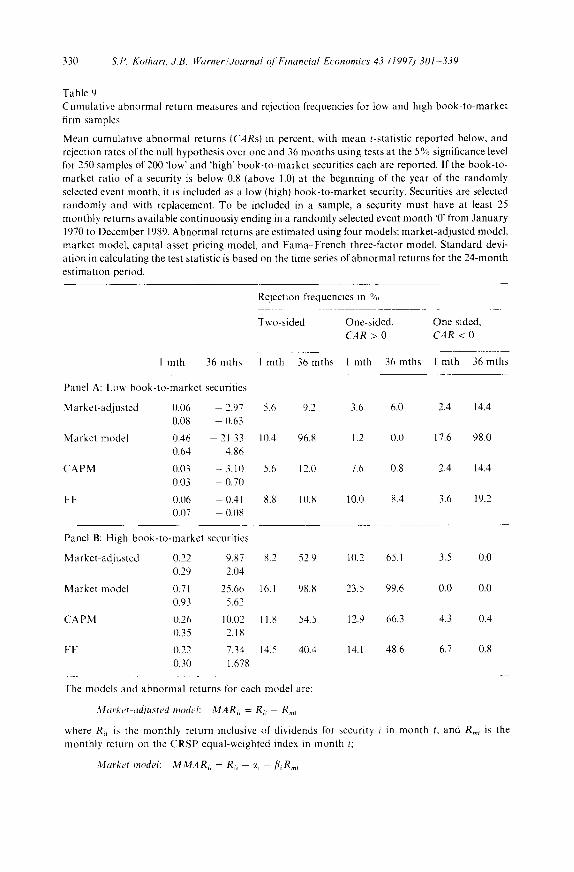
Table 9 shows that the estimated average abnormal performance is systemati- cally negative for the low book-to-market samples (panel A), and it is positive for the high book-to-market samples (panel B). From panel A, the 36-month market-adjusted and CAPM CARs are about - 3 % for the low book-to- market samples using the market-adjusted and CAPM benchmarks. The CARs using the market model are highly negative. Since the low book-to-market firms assumed that status in part because of their unusually good performance during the estimation period, their market model alphas are systematically positive, about 0.4% per month. Consequently, the highly negative market model CARs are due almost entirely to the estimated large, positive alphas. The FF three- factor model produces only a modest 36-month negative abnormal performance of -0 .41%. From the right most column in panel A. all four models show negative abnormal performance too frequently at the end of three years. The CAPM and market-adjusted models each show negative abnormal performance 14.4% of the time, whereas the FF three-factor model's rejection rate is 19.2%.
From panel B, the abnormal performance measures and rejection rates are much more dramatic for the high book-to-market portfolios. The 36-month mean abnormal performance ranges from about 7.3% using the FF three-factor model to 25.7% using the market model. One-tailed tests at the 5% significance level show positive abnormal performance in 48.6%, to 99.6% of the samples.
Overall, the results in Table 9 suggest that long-horizon tests using nonran- dom samples strongly show either positive or negative abnormal performance when none is present. The observed abnormal performance of book-to-market samples using the market-adjusted, CAPM, and market-model measures of abnormal returns is not surprising. Fama and French (1992) and others have documented a positive relation between average returns and book-to-market ratios that cannot be explained using the CAPM. Interestingly, however, even the FF three-factor model shows abnormal performance too often. This suggests inadequacies either in existing benchmark models or in the implementation of these models in long-horizon studies.
Simulations using large- and small-firm samples yield results similar to those using nonrandom book-to-market firm samples in that the average abnormal performance for the small- and large-firm samples is quite different. In the 1980s,
330 S,P. Kothari, J.B. Warner/Journal o/ 'Financial Economics 43 (1997) 301-339
Table 9 Cumulative abnormal return measures and rejection frequencies for low and high book-to-market firm samples
Mean cumulative abnormal returns {CARs} in percent, with mean t-statistic reported below, and rejection rates of the null hypothesis over one and 36 months using tests at the 5% significance level for 250 samples of 200 qow' and 'high" book-to-market securities each are reported. If the book-to- market ratio of a security is below 0.8 (above 1.0) at the beginning of the year of the randomly selected event month, it is included as a low (high) book-to-market security. Securities are selected randomly and with replacement. To be included in a sample, a security must have at least 25 monthly returns available continuously ending in a randomly selected event month '0' from January 1970 to December 1989. Abnormal returns are estimated using four models: market-adjusted model, market model, capital asset pricing model, and Fama French three-factor model. Standard devi- ation in calculating the test statistic is based on the time series of abnormal returns for the 24-month estimation period.
Rejection frequencies in %
Two-sided One-sided, One sided, CAR > 0 CAR < 0
1 mth 36mths 1 mth 36mths l mth 36mths I mth 36mths
Panel A: Lo~ book-to-market securities
Market-adjusted 0.06 2.97 5.6 9.2 3.6 6.0 2.4 14.4 0.08 0.63
Market model 0.46 - 21.33 10.4 96.8 1.2 0.0 IZ6 98.0 0.64 4.86
CAPM 0.03 - 3.10 5.6 12.0 7.6 0.8 2.4 14.4 0.03 - 0.70
FF 0.06 - 0.41 8.8 10.8 10.0 8.4 3.6 19.2 0.07 0.08
Panel B: High book-to-market securities
Market-adjusted 0.22 9.87 8.2 52.9 10.2 65.1 3.5 0.0 0.29 2.04
Market model 0.71 25.66 16.1 98.8 23.5 99.6 0.0 0.0 0.93 5.62
CAPM 0.26 10.02 11.8 54.5 12.9 66.3 4.3 0.4 0.35 2.18
FF 0.22 7.34 14.5 40.4 14.1 48.6 6.7 0.8 0.30 1.678
The models and abnormal returns for each model are:
Marker-adjusted mode[: MARir = R,.t R,,,
where Ri, is the monthly return inclusive of dividends for security i in month t, and R,,, is the monthly return on the CRSP equal-weighted index in month t;
Market model: /~J.'~[,4Rit - Ri, ~¢ - fiiR,,,
S.P. Kothari, J.B. Warner;Journal Of Financial Economics 43 (1997) 301 339 331
however, both small- and large-firm samples exhibit positive CARs at the end of 36 months, with large firms' CARs exceeding those of the small firms. This is consistent with large firms outperforming the small firms in the 1980s.
7.2. Matched-portlolio-based tests
Matched-portfolio-based tests compare the average return on the sample firms to that on a portfolio of firms matched on characteristics such as size and book-to-market. Our FF three-factor-model-based test is one way of adjusting for size and book-to-market, but a matched-portfolio approach is an alternative. Matched-portfolio-based tests do not require pre-event data for parameter estimation. Evidence on these tests is contained in three recent papers.
Ikenberry, Lakonishok, and Vermaelen (1995). Properties of matched-port- folio tests can be inferred from the Ikenberry, Lakonishok, and Vermaelen event study of open-market repurchases. The results are quite similar to those re- ported here in that matched portfolios' mean long-horizon abnormal returns are
table 9 (continued)
where :~, and [:~ are market model parameter estimates obtained by regressing mon th ly re turns for security i on the equal-weighted market returns over the 24-month estimation period from event month 24 to - 1:
CAPM: CAPMARi, = Ri, Rr, -- [';i[R,,,, Rlr ]
where fi, is from the CAPM regression model [i.e., slope from a regression of ( R i , - R;,) on (R.,, - Rs,) using 24 monthly observations for the estimation period], and R s, is one-month T-bill re turn used as a proxy for risk-free return:
FF: FFMARi, Ri, - R f, -. fiil [Rm, - Rr,] - [ ~ i 2 HML~ - [ ~ i 3 SMB,
where HML, and SMB, are the Fama French book-to-market and size factor returns and fl~l, fl~2, and fl~3 are estimated by regressing security i's monthly excess re turns on the monthly market excess returns, book-to-market, and size factor re turns for the 24 month estimation period.
The test statistic for the event month is (illustrated using market-adjusted returns):
l x'
MARpt (;{MAR m) where MAR.,, = 7~ ~" MAR~,. i = l
[ ~ ,4uIMARv) 2 23 ] . . . . [ 1 a{MARp,) - t --2a {M,4R,,~ , 4cg(M.4Rp) = .24,=~'_ MARp,.
and N, is the number of securities that are available in month ~
The test statistic to assess lhe statistical significance of abn o rma l performance over a T-month period beginning with the event month '0" is
CMARe?- 1 L a(MARpI . TI : where CMARp? = ,=o~ M,4Rp~.
332 S.P. Kothari, ,LB. Warner~Journal q[Financial Economics 43 (1997) 301 339
systematically nonzero. This provides an independent robustness check. In their paper, the sample buy-and-hold abnormal return is defined as the difference between the buy-and-hold return and the corresponding return on a portfolio of securities matched by book-to-market, size, and event date. To assess statistical significance, this difference is compared to a bootstrap distribu- tion of buy-and-hold abnormal returns. This bootstrap distribution consists of buy-and-hold abnormal returns on 1,000 samples of randomly selected secur- ities also matched by size, book-to-market, and event date to the sample securities.
The mean four-year buy-and-hold abnormal return from the bootstrap distri- bution is positive, and the mean of the bootstrap distribution for low book-to- market firms is negative. 4 These results would be surprising for well-behaved performance measures, but are not surprising in light of our previous results. The use of a bootstrap distribution represents a state-of-the-art procedure to recognize and attempt to adjust for such systematic biases in assessing statistical significance. It remains an open question whether such procedures are appro- priate. This is discussed in Section 8.2.
Barber and Lyon (1996a, b). In the Barber and Lyon simulations of long- horizon event-study procedures, a wide variety of matching procedures are examined, and the main focus is parametric statistical tests. There is dramatic evidence of misspecification, and we view the general tenor of the results as similar to ours. Barber and Lyon demonstrate that many of the commonly used matching procedures are poorly specified and abnormal return estimates can be systematically nonzero. Further, seemingly minor changes in experimental fea- tures can have a major impact on specification. These include the benchmark for measuring abnormal returns, cumulation procedures, the populations from which securities are sampled (e.g., NYSE/AMEX versus NASDAQ), or calendar time periods. Barber and Lyon isolate one parametric procedure that may be well-specified, specifically to calculate abnormal returns as the buy-and-hold return on a sample firm less the buy-and-hold return on a control firm with similar size and book-to-market characteristics. However, they do not demon- strate the robustness of this procedure to samples with other characteristics (e.g., earnings yield or past sales growth). Further, conclusions about whether a par- ticular test is well-specified seem quite fragile, given their other evidence. This reinforces both our arguments and those of Ikenberry, Lakonishok, and Ver- maelen (1995) that bootstrap procedures might be a promising way to minimize test statistic misspecification.
SSee their Fig. 2. Although not reported in their paper, the mean four-year bootstrap buy-and-hold abnormal return for their full sample is 1.95%, with 64.9% positive observations. For the lowest book-to-marke! quintile sample, the mean return for the bootstrap distribution is - 4 . 3 1 % . We thank the authors for providing us with these details in private correspondence.
S.P. Kothari, J.B. Warner~Journal of Financial Economics 43 (1997) 301 339 333
7.3. Other variations in test procedures
We also perform numerous simulations by experimenting with different estimation periods and different populations of firms from which samples are selected. In particular, we use a 24-month post-test period as the estimation period, and also the combination of 24-month pre- and post-test periods (i.e., a total of 48 months) as the estimation period. The use of the post-test period to estimate model parameters requires that securities must survive the entire 36-month test period and the post-test estimation period to be included in the random samples. We also repeat the baseline simulations using only the stocks for which book value of equity data at the beginning of the year of the event month are available on COMPUSTAT. The tenor of the results from these simulations is similar to that discussed in the paper.
8. Implications for empirical research
8.1. Existing regularities. Survey and interpretation
Table 10 summarizes existing results on long-horizon abnormal performance following events. We identify several empirical regularities in these event studies. As discussed below, the general patterns seem consistent with misspecification, but no claim is made that misspecification (rather than mispricing) drives the results.
Persistence. From Table 10, reported abnormal performance persists for years following 12 different types of events. Horizons over which performance is tracked generally range from 24 to 60 months, and the abnormal performance is generally significant over the entire period. 5 Persistence for the entire three-year tracking period is detected in all of our simulations. Thus, persistence reported in the literature is quite consistent with misspecification, and inconsistent with mispricing unless the mispricing lasts beyond the tracking period. Further, reports of persistence in so many different studies does not imply long-lived mispricing if the common factor driving the results is test statistic misspecifica- tion.
Positive versus negative abnormal performance. Reported post-event effects are both positive and negative, depending on the type of event. From Table 10,
SConsistent with persistence, abnormal performance for the final year of the horizon is sometimes significant (e.g.. Speiss and Attteck-Graves, 1995, Table 2: Ritter, 1991, Table I1: Dharan and lkenberry. 1995, Table 11), but the significance of final-year performancc is often not reported and this performance is sometimes insignificant (e.g.. Agrawal, Jaffe, and Mandelker, 1992, Table li.
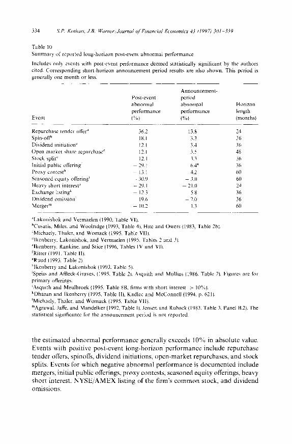
334 S.P. Kothari. ,LB. Warner~Journal of Financial Economics 43 (1997) 301 339
Table 10 Summary of reported long-horizon post-event abnormal performance
Includes only events with post-event performance deemed statistically significant by the authors cited. Corresponding short-horizon announcement period results are also shown. This period is generally one month or less.
Event
Announcement- Post-event period abnormal abnormal Horizon performance performance length (%) (%) (months)
Repurchase tender offer" 36.2 13.8 24 Spin-off ° 18.1 3.3 36 Dividend initiation ~ 12. I 3.4 36 Open market share repurchase d 12.1 3.5 48 Stock split ~ 12.1 3.3 36 Initial public offering r - 29.1 6.4 g 36 Proxy contest h - 13.1 4.2 60 Seasoned equity offering ~ - 30.9 3.0 60 Heavy short interest j - 29.1 21.0 24 Exchange listing k 12.3 5.8 36 Dividend omission ~ 19.6 - 7.0 36 Merger m 10.2 1.3 60
~Lakonishok and Vermaelen (1990, Table VI). bCusatis, Miles. and Woolridge (1993, Table 4), Hite and Owers (1983, Table 2b), ~Michaely, Thaler, and Womack (1995, Table VII). qkenberry, Lakonishok, and Vermaelen (1995, Tables 2 and 3). qkenberry, Rankine, and Stice (1996, Tables IV and VI). fRitter (1991, Table I1). gRuud 11993, Table 2). hlkenberry and Lakonishok (1993, Table 5). 'Speiss and Affteck-Graves, (1995, Table 2i, Asquith and Mullins (1986, Table 2!. Figures are for primary offerings. JAsquith and Meulbroek (1995, Table 8B, firms with short interest > 10%). kDharan and Ikenberry (1995, Table II), Kadlec and McConnel111994, p. 62t). ~Michaely, Thaler, and Womack (1995, Table VII). mAgrawal, Jaffe, and Mandelker (1992, Table I), Jensen and Ruback (1983. Table 3, Panel B.2). The statistical significance for the announcement period is not reported.
the estimated abnormal performance generally exceeds 10% in absolute value. Events with positive post-event long-horizon performance include repurchase tender offers, spinoffs, dividend initiations, open-market repurchases, and stock splits. Events for which negative abnormal performance is documented include mergers, initial public offerings, proxy contests, seasoned equity offerings, heavy short interest, NYSE/AMEX listing of the firm's common stock, and dividend omissions.
S.P. Kothari, J.B. l~2lrner/Journal qf Financial Economics 43 (1997) 301 339 335
Both large positive and large negative abnormal performance are quite consistent with misspecification. For randomly selected securities, our simula- tions show a strong tendency to find positive abnormal performance too often, with mean abnormal performance often exceeding 10%. For nonrandomly selected securities (e.g., firms with unusual book-to-market ratios), we document that the tendency to find both positive and negative abnormal performance can be more pronounced. As discussed in Section 7.2, however, the direction of the bias toward finding positive or negative abnormal performance is quite sensitive to the characteristics of a given sample. Thus, it is difficult to generalize about whether results for a particular study are driven by an overrejection bias, or whether they occur in spite of an underrejection bias. For this reason, it seems premature to claim that reported results for specific events can be attributed to misspecification of long-horizon tests. Investigation of this possibility would require additional study, specifically replication of existing studies using im- proved procedures such as bootstrap (see below). Further. a few long-horizon studies use bootstrap procedures but still find abnormal performance (e.g., Ikenberry, kakonishok, and Vermaelen, 1995; Ikenberry, Rankine, and Stice, 1996). This makes it harder to dismiss all long-horizon results as a consequence of parametric test misspecification.
Underreaction versus overreaction. For each type of event, Table 10 compares abnormal performance in both the event and post-event periods. There is no obvious sign pattern. In eight of 12 events, the long-horizon post-event abnor- mal performance is in the same direction as the announcement effect, but in three events it is in the opposite direction. Mergers are excluded because the announcement effect is not clearly statistically significant. The lack of a clear sign pattern is important for two reasons. First, long-horizon misspecification implies no obvious correlation between the sign of an announcement effect and that of the corresponding multi-year post-event effect, and the observed sign pattern seems consistent with misspecification. Second, across the studies there is no strong pattern of either stock market underreaction or overreaction to events. This does not support any behavioral model (e.g., contrarianj in which security price reactions to events are biased in a particular direction.
Data snooping biases and benchmark correlations. In several instances, pub- lished results showing long-horizon abnormal returns have led to follow-up studies in which the result was shown to be sensitive to test methodology. For example, in reexamining post-merger negative performance of bidders, Franks, Harris, and Titman (1991) argue that previous findings are due to benchmark errors. Bray and Gompers (1995) re-examine post-IPO performance and con- clude that underperformance is concentrated in a small number of firms, and is sensitive to the weighting of the observations.
In the presence of strong abnormal performance, it would be surprising to find that test results are highly dependent on the choice of methodology. In the absence of abnormal performance, however, conflicting results are more likely
336 S.P. Kothari, J.B. Warner/Journal ~/'Financial Economics 43 (1997) 301 339
because event-study test statistics are not perfectly positively correlated across procedures (see Brown and Warner, 1980, Table 10). Further, for a given sample, the probability of finding a 'significant' result using a battery of different tests will be much higher than the significance level of any one test. Previous simulations thus understate the likelihood of detecting abnormal performance because the simulations examine each procedure individually and ignore the correlation structure of the tests.
To provide evidence on this type of data-snooping bias, we report additional details of our previous tests. For example, in panel A of Table 1, tests with four different benchmarks show rejection rates of roughly 20% to 30% for each benchmark using a two-tailed test at the 5% significance level. When all four benchmarks are simultaneously applied, the percentage of samples in which the null hypothesis is rejected using at least one test jumps to 48.4%. This figure serves to further reinforce the conclusion that long-horizon tests must be interpreted with great care.
8.2. Be t t e r l ong-hor i zon tests
A few long-horizon studies finding abnormal performance use nonparametric procedures. Although we do not study these alternative methods here, they seem like a promising alternative to the parametric procedures examined here. Nonparametric procedures appear to have fewer potential problems, and conclusions based on these procedures seem less likely to be due to misspecifica- tion. Our study helps identify potential sources of misspecification with these procedures, and how to tailor nonparametric procedures to avoid misspecifica- tion.
Bootstrap procedures, such as those employed by lkenberry, Lakonishok, and Vermaelen (1995), could be used to address biases in both the measure of abnormal performance and the standard deviation. As discussed earlier, these procedures use return data for random samples of matched nonevent firms to construct a bootstrap distribution of long-horizon abnormal returns under the null hypothesis. The difficulty is that firms used to construct the bootstrap distribution must be correctly matched to the sample firms. Merely being of similar size and book-to-market ratio may not be sufficient. As shown earlier, many biases are survival-related and arise in part because of event-study data requirements, and are poorly understood. Unless the firms used to construct the bootstrap distribution have similar biases to the sample firms, correct specifica- tion is not guaranteed. Recent post-merger long-horizon work (by Brown and Da Silva Rosa, 1995) incorporates survival-related controls and argues for their importance.
Simple nonparametric sign tests are sometimes used in long-horizon studies (e.g., Spiess and Affleck-Graves, 1995). These tests seem straightforward, but can still suffer from some of the difficulties of parametric procedures. As discussed
S.P. Kothari. JB. Wcwner/Journal Of Financial Economics 43 (1997) 301 339 337
earlier, the empirical distribution of buy-and-hold abnormal returns is skewed. It seems likely that long-horizon test specification is very sensitive to this characteristic. With skewness, the proportion of positive abnormal returns can depart significantly from 50% under the null hypothesis. With monthly data, it is well-known that the degree of misspecification in sign tests is severe (Brown and Warner, 1980, Table 2). To be correctly specified, nonparametric tests must be designed to explicitly take skewness into account, perhaps using bootstrap- type procedures to assess the degree of skewness under the null hypothesis.
9. Conclusions and recommendations
Previous work suggests that long-horizon event study tests will have low power (Brown and Warner, 1980). We find that parametric long-horizon tests will often indicate abnormal performance when none is present. This further reduces one's confidence in the reliability of inferences from long-horizon studies, and serves to bolster previous warnings that the interpretation of long-horizon tests requires extreme caution. Further, the general impression that long-horizon procedures can yield bizarre results is reinforced in other work. Both the simulation study of Barber and Lyon (1996a) and simulation results reported in the event study of Ikenberry, Lakonishok, and Vermaelen (1995) convey a similar impression.
Researchers can build on our work in several specific ways. First, better tests should be used to replicate existing long-horizon studies. From a brief survey of the literature presented here, this seems like a significant and growing area. At this point, however, it is unknown whether existing results are due to mispricing or to test misspecification.
Second, we offer a positive prescription for better long-horizon event studies. Nonparametric procedures, such as bootstrap, seem like a promising framework for alternative tests which can potentially reduce misspecification. Since boot- strap is nothing more than doing Brown and Warner (1980, 1985) type simula- tions to estimate p-values, the technology is not new. Our recommendation is related to Barber and Lyon (1996a). They argue that some types of parametric matched-portfolio tests are well specified and yield well-behaved abnormal performance measures. A concern from both our work and theirs (see Barber and Lyon, 1996a,b), however, is that conclusions from simulation studies can themselves be sensitive to experimental design. To allay such concerns, non- parametric and bootstrap tests could easily be coupled with matched-portfolio- based abnormal performance measures to more accurately calibrate statistical significance.
Third, while we have documented several survival-related biases, the exact nature of these biases is still not fully understood. Further analysis of survival- related biases seems clearly fruitful. This would, at the least, enhance our
338 S.P. Kothari. ,LB. Warner/Journal (?l Financial Economics 43 (1997) 301 339
understanding of when these biases are likely to be important and when they are likely to be unimportant. Our analysis suggests how even bootstrap procedures are potentially subject to these biases
Finally, we have focused on long-horizon returns in only one context, event studies. Measuring portfolio long-horizon performance in calendar time, for example in the mutual fund context, involves many related issues. The relevance of our findings to mutual fund portfolio performance is an area we are currently investigating.
References
Agrawal, Anup, Jeffrey F. Jafl'e. and Gershon N. Mandelker, 1992, The post-merger performance of acquiring firms: A reexamination of an anomaly, Journal of Finance 47, 1605 162l.
Asquith, Paul and Lisa Meulbroek, 1995, An empirical investigation of short interest, Working paper (Massachusetts Institute of Technology, Boston, MA).
Asquith. Paul and David W. Mullins, 1986, Equity issues and offering dilution, Journal of Financial Economics 15, 61 89.
Ball, Ray, 1978. Anomalies in relationships between securities' yields and yield-surrogates, Journal of Financial Economics 6, 103 126.
Ball. Ray and S.P. Kothari, 1989, Nonstationary expecled returns: Implications for tests of market efficiency and serial correlation in returns, Journal of Financial Economics 25, 51 74.
Ball, Ray, S.P. Kothari, and Jay Shanken, 1995. Problems in measuring portfolio performance: An application to contrarian investment strategies, Journal of Financial Economics 38, 79 107.
Barber, Brad M. and John D. Lyon. 1996a~ [)electing long-run abnormal stock returns: The empirical power and specification of test statistics, Journal of Financial Economics, this issue.
Barber, Brad M. and John D. Lyon, 1996b, How can long-run abnormal stock returns be both positively and negatively biased?, Working paper iUniversity of California, Davis, CAl.
Bernard, Victor L., Jacob Thomas, and James Wahlen, 1995, Accounting-based stock price anomalies: Separating market inefficiencies from research design flaws, Working paper (Univer- sity of Michigan, Ann Arbor, MI).
Blume. Marshall and Robert F. Stambaugh, 1983, Biases in computed returns: An application to the size effect, Journal of Financial Economics 12, 387 404.
Brav~ Alon and Paul A. Gompers, 1995, Myth or reality? The long-run underperformance of initial public offerings: Evidence from venture and nonvenlure capital-backed companies, Working paper (University of Chicago. Chicago, ILl.
Brown, Philip and Raymond l)a Silva Rosa, 1995, Returns to shareholders of firms involved in Australian corporate takeovers: A re-examination, Working paper (University of Western Australia. Cityl,
Brown. Stephen J. and Jerold B. Warner, 1980, Measuring security price performance. Journal of Financial Economics 8, 205 258.
Brown, Stephen J. and Jerold B. Warner, 1985. Using daily stock returns: The case of event studies, Journal of Financial Economics 14, 3 31.
Brown, Stephen J., William N. Goetzmann, and Stephen A. Ross, 1995, Survival, Journal of Finance 50. 853 873.
Chan. K.C.. 1988, On the contrarian investment strategy. Journal of Business 61, 147 163. Choprm Navim Josef Lakonishok, and Jay R Ritter, 1992, Measuring abnormal performance: Do
stocks overreact'?, Journal of Financial Economics 31, 235 268. Conrad. Jennifer and Gautam Kaul, 1993, Long-term market overreaction or biases in computed
returns, Journal of Finance 48, 39~ 63.

S.P. Kothari. J,B. Warner'Journal ~/'Financial Economics 43 (1997) 301 339 339
Cusatis. Patrick J., James A. Miles, and J. Randall Woolridge, 1993, Restructuring through spinoffs: The stock market evidence, Journal of Financial Economics 33, 293 31 l.
Desai, Hemang and Prem C. Jain, 1995, Long-run common stock returns following stock splits and stock dividends, Working paper (Tulane University, New Orleans, LA).
Dharan, Bala G. and David L. lkenberry, 1995, The long-run negative drift of post-listing stock returns, Journal of Finance 50, 1547 1574.
Dimson, Elroy and Paul Marsh, 1986, Event study methodologies and the size effect: The case of U K press recommendations, Journal of Financial Economics 17. 113 142.
Fama, Eugene F.. 1991, Efficient capital markets 11, Journal of Finance 46, 1575-1617. Fama, Eugene F. and Kenneth R. French, 1992, The cross-section of expected returns, Journal of
Finance 47, 427M.65. Fama, Eugene F. and Kenneth R. French, 1993, Common risk factors in the returns on stocks and
bonds, Journal of Financial Economics 33, 3 56. Fama, Eugene F. and Kenneth R. French, 1995, Size and bouk-to-market factors in earnings and
returns, Journal of Finance 50, 131 155. Franks, Julian, Robert Harris. and Sheridan Titman, 1991, The postmerger share-price performance
of acquiring firms, Journal of Financial Economics 29, 81 96. Hite, Gailen L. and James E. Owers, 1983, Security price reactions around corporate spin-off
announcements, Journal of Financial Economics 12, 409436. Ikenberry. David L. and Josef Lakonishok, 1993, Corporate governance through the proxy contests:
Evidence and implications, Journal of Business 66, 405 436. lkenberry, David, Josef Lakonishok, and Theo Vermaelen, 1995. Market underreaction to open
market share repurchases, Journal of Financial Economics 39, 181 208. lkenberry, David, Graeme Rankine, and Earl K. Stice, 1996, What do stock splits really signal'?,
Unpublished manuscript (Rice University, Houston, TXI, Jain, Prem C.. 1982, Cross-sectional association between abnormal returns and firm specific
variables, Journal of Accounting and Economics 4, 205 228. Jensen, Michael C. and Richard S. Ruback, 1983, The market for corporate control: The scientific
evidence, Journal of Financial Economics 1 l, 5 50. Kadlec, Gregory B. and John J. McConnell, 1994, The eft'cot of market segmentation and illiquidity
on asset prices: Evidence from exchange listings, Journal of Finance 49, 611 636. Keim, Donald B., 1989, Trading patterns, bid-ask spreads, and estimated security returns: The case
of common stocks at calendar turning points, Journal of I-inancial Economics 25, 75 97, Kothari, S.P., Jay Shanken, and Richard G. Sloan, 1995, Another look at the cross-section of
expected returns. Journal of Finance 50, 185 224. Lakonishok, Josef and Theo Vermaelen, 1990, Anomalous price behavior around repurchase tender
offers, Journal of Finance 45, 455 477. Loughran, Tim and Jay R. Ritter, 1995, The new issues puzzle, Journal of Finance 50, 23 51. Maddala, G. S., 1988, Introduction to econometrics (Macmillan, New York, NY). Michaely, Roni, Richard H. Thaler, and Kent L. Womack, 1995, Price reactions to dividend
initiations and omissions: Overreaction or drift?, Journal of Finance 50, 573 608. Ritter, Jay R., 1991, The long-run performance of initial public offerings. Journal of Finance 46,
3 28. Roll, Richard, 1983, On computing mean returns and the small lirm premium, Journal of Financial
Economics 12, 371 386. Ruud, Judith S., 1993. Underwriter price support and the IPO underpricing puzzle, Journal of
Financial Economics 34, 135 151. Schwert, G. William, 1983, Size and stock returns, and other empirical regularities, Journal of
Financial Economics 12.3-12. Speiss, D. Katherine and John Affleck-Graves. 1995, Undcrperfurmance in long-run stock returns
following seasoned equity offerings, Journal of Financial Economics 38, 243 267.