Embed Size (px)
Citation preview

Measuring Illegal Activity and the Effects of Regulatory Innovation:
Tax Evasion and the Dyeing of Untaxed Diesel
Justin Marion †
Erich Muehlegger ‡
March 2008
Abstract
This paper examines tax evasion in the diesel fuel market. Diesel fuel used for on-roadpurposes is taxed, while other uses are untaxed, creating an incentive for firms and individualsto evade on-road diesel taxes by purchasing untaxed diesel fuel and then using it for on-roaduse. We examine the effects of a federal regulatory innovation in October 1993, the addition ofred dye to untaxed diesel fuel at the point of distribution, which significantly lowered the cost ofregulatory enforcement. We find that sales of diesel fuel rose 26 percent following the regulatorychange while sales of heating oil, which is an untaxed perfect substitute, fell by a similar amount.The effect on sales was higher in states with higher tax rates and in states likely to have higheraudit costs. We also find evidence that heating oil sales are less responsive to demand factorssuch as temperature prior to the dye program, indicating that a significant fraction of pre-dyesales was illegitimate. Furthermore, we find a pattern of price and tax elasticities consistentwith innovation in new evasion techniques subsequent to the regulatory change. Finally, weestimate that the elasticity of tax revenues with respect to the tax rate was 0.60 prior to thedye program, yet would have been 0.85 in the absence of evasion.
∗The authors thank Raj Chetty, Ed Glaeser, Monica Singhal, Christopher Snyder, and seminar participants at theFederal Trade Commission, UC Santa Cruz, International Industrial Organization Conference, Tufts, UC Berkeley,UC Davis, Texas A&M, the University of Oklahoma, Syracuse, MIT, UC Merced, and the National Tax Associationfor helpful comments and conversations.
†University of California, Santa Cruz. [email protected]‡John F. Kennedy School of Government, Harvard University. Erich [email protected].
1

1 Introduction
Tax evasion and tax collection are important elements of fiscal policy. Lack of compliance with
tax laws are likely to alter the distortionary costs of raising a given level of government revenue
and may affect the distributional consequences of a given tax policy. Furthermore, resources
spent evading taxes represent a deadweight loss to the economy. Despite the central importance
of tax evasion in public finance, our understanding of the degree of evasion and its response to
the rate of taxation and government enforcement is limited.
Detecting tax evasion and estimating how it responds to tax and enforcement policy have
traditionally been difficult since those engaging in evasion wish to keep this behavior concealed.
Furthermore, disentangling the effects of tax rates and audit intensity from other unobserved fac-
tors is not straightforward. Audit intensity is likely to be endogenously related to the propensity
to evade, as auditors focus collection resources toward groups of taxpayers likely to evade. Also,
variation in tax rates across individuals or firms is often correlated with evasion opportunities.
For instance, higher income individuals face a higher marginal tax rate and at the same time
may have more income from sources that are easier to conceal. The value of providing empirical
evidence regarding these questions is high, as even theoretically the response of evasion to tax
rates is not clear.1
The diesel market provides an interesting setting to study tax evasion. The taxation of
diesel fuel varies significantly by use. Despite being virtually identical to the diesel used for
on-road purposes, diesel fuel consumed for off-road use such as residential heating, industrial
use, farming or off-road travel is untaxed. In 2005, consumers using diesel fuel for on-road
purposes faced federal highway taxes of 24.4 cents per gallon in addition to state highway taxes
that range from 8 to 32.1 cents per gallon. Some localities tax on-road diesel as well, altogether
placing the tax burden at over 50 cents per gallon in many states. The close substitutability
and differential taxation of on-road and off-road diesel create strong incentives for firms to evade
diesel taxation by purchasing untaxed diesel fuel and using or reselling it for on-road use.
In this paper, we consider the impacts on tax evasion of a regulatory innovation that greatly
decreased the cost of monitoring compliance with on-road diesel fuel taxes. In October 1993, the
Federal Highway Administration began adding red dye to untaxed diesel fuel. The dye allows
inspectors to readily check for untaxed diesel through simple visual inspection, reducing the cost
of auditing for regulators and increasing the cost of achieving a given level of diesel tax evasion
1Allingham and Sandmo (1972) analyze the evasion decision, finding that evasion is positively related to tax rates.However, Yitzhaki (1974) shows that this result depends on the nature of penalty imposed on audited evaders andon the preferences of potential evaders.
2
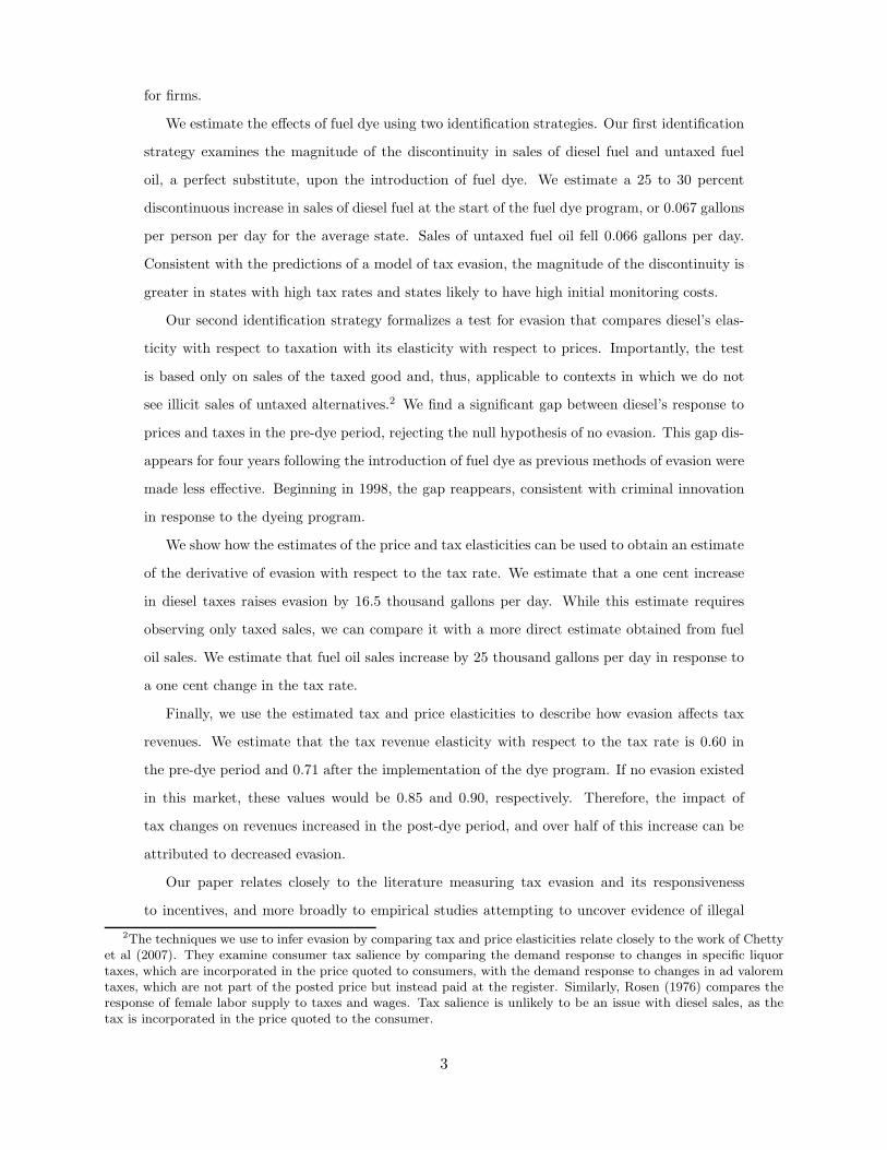
for firms.
We estimate the effects of fuel dye using two identification strategies. Our first identification
strategy examines the magnitude of the discontinuity in sales of diesel fuel and untaxed fuel
oil, a perfect substitute, upon the introduction of fuel dye. We estimate a 25 to 30 percent
discontinuous increase in sales of diesel fuel at the start of the fuel dye program, or 0.067 gallons
per person per day for the average state. Sales of untaxed fuel oil fell 0.066 gallons per day.
Consistent with the predictions of a model of tax evasion, the magnitude of the discontinuity is
greater in states with high tax rates and states likely to have high initial monitoring costs.
Our second identification strategy formalizes a test for evasion that compares diesel’s elas-
ticity with respect to taxation with its elasticity with respect to prices. Importantly, the test
is based only on sales of the taxed good and, thus, applicable to contexts in which we do not
see illicit sales of untaxed alternatives.2 We find a significant gap between diesel’s response to
prices and taxes in the pre-dye period, rejecting the null hypothesis of no evasion. This gap dis-
appears for four years following the introduction of fuel dye as previous methods of evasion were
made less effective. Beginning in 1998, the gap reappears, consistent with criminal innovation
in response to the dyeing program.
We show how the estimates of the price and tax elasticities can be used to obtain an estimate
of the derivative of evasion with respect to the tax rate. We estimate that a one cent increase
in diesel taxes raises evasion by 16.5 thousand gallons per day. While this estimate requires
observing only taxed sales, we can compare it with a more direct estimate obtained from fuel
oil sales. We estimate that fuel oil sales increase by 25 thousand gallons per day in response to
a one cent change in the tax rate.
Finally, we use the estimated tax and price elasticities to describe how evasion affects tax
revenues. We estimate that the tax revenue elasticity with respect to the tax rate is 0.60 in
the pre-dye period and 0.71 after the implementation of the dye program. If no evasion existed
in this market, these values would be 0.85 and 0.90, respectively. Therefore, the impact of
tax changes on revenues increased in the post-dye period, and over half of this increase can be
attributed to decreased evasion.
Our paper relates closely to the literature measuring tax evasion and its responsiveness
to incentives, and more broadly to empirical studies attempting to uncover evidence of illegal
2The techniques we use to infer evasion by comparing tax and price elasticities relate closely to the work of Chettyet al (2007). They examine consumer tax salience by comparing the demand response to changes in specific liquortaxes, which are incorporated in the price quoted to consumers, with the demand response to changes in ad valoremtaxes, which are not part of the posted price but instead paid at the register. Similarly, Rosen (1976) compares theresponse of female labor supply to taxes and wages. Tax salience is unlikely to be an issue with diesel sales, as thetax is incorporated in the price quoted to the consumer.
3

activity. Several approaches have been taken in prior literature to measure tax evasion. An
indirect approach involves observing aggregate quantities such as currency demand or national
income and product accounts and inferring evasion from these quantities.3 A second approach
utilizes cross-sectional variation across taxpayers in observed levels of compliance using the
Taxpayer Compliance Monitoring Project (TCMP), which describes the outcome of IRS audits
of randomly chosen tax returns.4 A third approach taken in the literature uses experimental
methods to investigate tax compliance and its response to tax rates and enforcement.5
The approach most closely related to that taken in our paper is that of Fisman and Wei
(2004), who examine the misclassification of Chinese imports from Hong Kong. They find that
the gap at the detailed good level between reported Chinese imports from Hong Kong and
reported exports from Hong Kong to China is largest for goods with high tax and tariff rates.
In a similar vein, Hsieh and Moretti (2006) uncover evidence of underpricing and bribes in Iraq’s
oil for food program by comparing prices charged by Iraq for oil with prices of close substitutes
sold on the world market. DellaVigna and La Ferrara (2006) use the response of the equity
prices of weapons manufacturers to armed conflict events to uncover evidence of illegal arms
sales.
Section 2 presents some background related to diesel markets and taxation and Section 3
describes a model of the firms’ tax evasion decision. Section 4 describes the data to be used. Sec-
tion 5 presents the primary empirical evidence, the response of sales to the dye program. Section
6 provides results implementing the test of evasion and derives estimates of the responsiveness
of evasion to tax rates. Section 7 concludes.
2 Regulatory Background
The taxation of diesel fuel varies by use. Diesel fuel used on-road is subject to federal highway
taxes of 18.4 cents per gallon and state highway taxes of 9 to 32.1 cents per gallon. Federal fuel
taxes are the primary source of funding for the Federal Highway Trust which funds infrastructure
3See for instance Gutmann (1977), Feige (1979) utilizes total dollar transactions relative to GDP, and Pommerehneand Weck-Hannemann (1996).
4Clotfelter (1983) finds a positive relationship between individuals’ marginal tax rates and the degree of evasion.Feinstein (1991) pools two different years to address the simultaneous relationship between income and marginaltax rates and finds a negative relationship between tax rates and tax evasion. Dubin and Wilde (1988) and Beron,Tauchen, and Witte (1992) find that increasing the chances of an IRS audit is associated with higher reported adjustedgross income.
5Slemrod, Blumenthal, and Christian (2001) study the distributional impact of tax evasion in an experiment whererandomly selected taxpayers were sent letters warning of close scrutiny of their tax returns. Treated low and middleincome taxpayers reported higher AGI than the control group, but treated higher income individuals reported less.Other experimental approaches include Wenzel and Taylor (2004) and Alm and McKee (2005)
4

investment. In addition, environmental regulations limit the amount of allowable sulfur content
of on-road diesel fuel.6 Diesel fuel consumed for farming or off-road travel, or as fuel oil for
residential, commercial or industrial boilers is not subject to highway taxes and is not required
to meet similar sulfur limits.
Variation in taxation and environmental stringency by use create strong incentives for firms
to evade taxation. Evaders purchase untaxed diesel fuel and use or resell it for on-road use
without paying the appropriate highway taxes. In the 1980’s, the most common method of
evasion was the “daisy chain”, in which a company would purchase untaxed diesel fuel and
resell the diesel fuel to an affiliate to make it more difficult to audit the transaction. The
affiliate would then resell the fuel to retail stations as diesel for which highway taxes had been
collected.7 In 1992, the Federal Highway Adminstration estimated that firms evaded between
seven and twelve percent of on-road diesel taxes, approaching $1.2 billion dollars of federal and
state tax revenue annually. While evasion was also a concern for other fuels, including gasoline,
kerosene and jet fuel, diesel fuel presents a special situation. Both taxable and non-taxable
uses are significant. In 2004, 59.6 percent of distillate sales to end users were retail sales for
on-highway use.8 This creates the incentive to develop evasion schemes for on-road diesel taxes,
as well as provides access to large quantities of untaxed diesel fuel.
In response to “daisy chain” evasion, the Internal Revenue Service (IRS) and the Envi-
ronmental Protection Agency (EPA) innovated. Beginning October 1, 1993, new regulations
required fuel dye be added to all diesel fuel not meant for on-highway use.9 Beginning January
1, 1994, the point of federal highway taxation for diesel fuel was moved to the wholesale termi-
nal. As a result, any untaxed diesel fuel sold at the wholesale terminal was required to be dyed
and consumption or sale of dyed fuel was made illegal. 10
The IRS and EPA regulations reduce the cost of enforcement, and increase the cost of
common evasion schemes like the “daisy chain.” Fuel dye allows regulators to randomly test
trucks through a simple visual inspection, substantially reducing the cost of monitoring. Moving
6From October 1993 to August 2006, the allowable sulfur content for on-highway diesel fuel was 500 parts permillion. Regulations did not constrain the sulfur content of diesel intended for other uses. Beginning September 1,2006, diesel sold for on-highway use must meet Ultra Low Sulfur Diesel Fuel requirements, with sulfur content notexceeding 15 ppm.
7For documented examples of evasion, see the Federal Highway Administration Tax Evasion Highlights.8Fuel Oil and Kerosene Sales Report, Energy Information Administration, 2004.9EPA regulations relating to sulfur content began Oct 1993. IRS regulations relating to diesel on which on-highway
taxes had not been collected were enacted as part of the Omnibus Budget Reconciliation Act of 1993 and began Jan1994.
10The federal penalty for consuming or selling dyed fuel (“red diesel”) for on-road use is the greater of $10 pergallon of fuel or $1000. In addition to penalties for evading federal taxes, individual states penalize firm caughtevading state taxes. Denison and Eger (2000) document fuel evasion penalties for a subset of states in 1997.
5
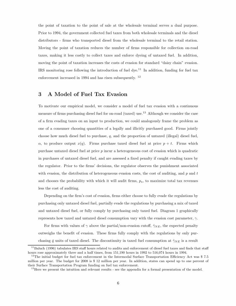
the point of taxation to the point of sale at the wholesale terminal serves a dual purpose.
Prior to 1994, the government collected fuel taxes from both wholesale terminals and the diesel
distributors - firms who transported diesel from the wholesale terminal to the retail station.
Moving the point of taxation reduces the number of firms responsible for collection on-road
taxes, making it less costly to collect taxes and enforce dyeing of untaxed fuel. In addition,
moving the point of taxation increases the costs of evasion for standard “daisy chain” evasion.
IRS monitoring rose following the introduction of fuel dye.11 In addition, funding for fuel tax
enforcement increased in 1994 and has risen subsequently. 12
3 A Model of Fuel Tax Evasion
To motivate our empirical model, we consider a model of fuel tax evasion with a continuous
measure of firms purchasing diesel fuel for on-road (taxed) use.13 Although we consider the case
of a firm evading taxes on an input to production, we could analogously frame the problem as
one of a consumer choosing quantities of a legally and illicitly purchased good. Firms jointly
choose how much diesel fuel to purchase, q, and the proportion of untaxed (illegal) diesel fuel,
α, to produce output x(q). Firms purchase taxed diesel fuel at price p + t. Firms which
purchase untaxed diesel fuel at price p incur a heterogeneous cost of evasion which is quadratic
in purchases of untaxed diesel fuel, and are assessed a fixed penalty if caught evading taxes by
the regulator. Prior to the firms’ decisions, the regulator observes the punishment associated
with evasion, the distribution of heterogeneous evasion costs, the cost of auditing, and p and t
and chooses the probability with which it will audit firms, pa, to maximize total tax revenues
less the cost of auditing.
Depending on the firm’s cost of evasion, firms either choose to fully evade the regulations by
purchasing only untaxed diesel fuel, partially evade the regulations by purchasing a mix of taxed
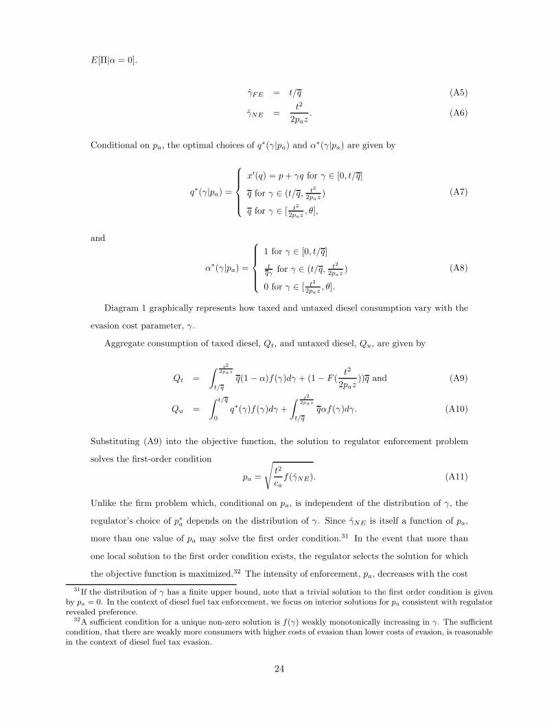
and untaxed diesel fuel, or fully comply by purchasing only taxed fuel. Diagram 1 graphically
represents how taxed and untaxed diesel consumption vary with the evasion cost parameter, γ.
For firms with values of γ above the partial/non-evasion cutoff, γ̂NE, the expected penalty
outweighs the benefit of evasion. These firms fully comply with the regulations by only pur-
chasing q̄ units of taxed diesel. The discontinuity in taxed fuel consumption at γ̂NE is a result
11Baluch (1996) tabulates IRS staff hours related to audits and enforcement of diesel fuel taxes and finds that staffhours rose approximately three and a half times, from 151,190 hours in 1992 to 516,074 hours in 1994.
12The initial budget for fuel tax enforcement in the Intermodal Surface Transportation Efficiency Act was $ 7.5million per year. The budget for 2008 is $ 12 million per year. In addition, states can spend up to one percent oftheir Surface Transportation Program funding on fuel tax enforcement.
13Here we present the intuition and relevant results - see the appendix for a formal presentation of the model.
6

of the fixed punishment. With a fixed penalty, purchasing an epsilon amount of untaxed fuel is
dominated by non-evasion. Partially-evading firms, with heterogeneous costs of evasion between
γ̂FE and γ̂NE , also purchase q̄ total units of diesel fuel. Partial-evaders purchase untaxed fuel
up until the point at which the marginal cost of evasion is equal to the tax rate. Firms below
the full/partial evasion cutoff, γ̂FE , only consume untaxed fuel. Fully-evading firms consume
untaxed fuel up until the point that marginal revenue is equal to price plus the marginal cost
of evasion, which is strictly less than the tax-inclusive price. As a result, fully-evading firms
consume more than q̄ units of diesel fuel.
Anticipating firms’ choices, the regulator endogenously chooses the probability with which
to audit, pa, to maximize tax revenues less auditing costs. Consistent with intuition, audit
intensity decreases with the cost of auditing, ca, and increases with the tax rate, t. An increase
in t increases the marginal benefit of auditing - an increase in ca increases the marginal cost of
auditing.
3.1 Empirical Predictions
We derive three sets of testable predictions which we would expect to hold if fuel tax evasion
exists and if the use of fuel dye reduces evasion: (1) predictions of the magnitude of the disconti-
nuity in sales before and after the introduction of the fuel dye, (2) predictions of the seasonality
in fuel oil sales pre- and post-dye, and (3) predictions of the price and tax elasticity of taxed
and untaxed diesel fuel.14
We derive predictions of the magnitude of the discontinuity in sales at the time of dye
introduction from the derivative of market demand for taxed and untaxed fuel, Qt and Qu,
with respect to the cost of auditing ca. In our context, fuel dye reduces the cost of monitoring
diesel fuel tax compliance. With lower auditing costs, the regulator optimally increases audit
intensity. As a result, we expect consumption of untaxed diesel to fall and consumption of
taxed diesel to rise as a result of the regulatory innovation. In addition, the theoretical model
predicts correlations between state characteristics and the magnitude of the discontinuity in
sales at the time of the fuel dye introduction. High state tax rates create greater incentive for
evasion as well as a greater change in enforcement following a decrease in audit costs. Thus,
our model predicts that the magnitude of the discontinuity in sales should be greater for high
tax jurisdictions than low tax jurisdictions. In addition, if monitoring is initially more difficult
in states with substantial markets for untaxed diesel fuel, we would expect the discontinuity to
14We include the formal derivation of the testable predictions in the appendix.
7
be greater in jurisdictions with high legal demand for untaxed diesel fuel.
A second set of testable predictions compare pre- and post-dye seasonality in fuel oil sales.
Seasonality of fuel oil demand differs substantially by use - residential demand for home heating
is greatest during the winter, while industrial and commercial demand exhibit little seasonality.
We expect illegal purchases of untaxed fuel oil, for use on-highway, to reduce seasonality in states
where a large proportion of households use fuel oil for home heating. In addition, if evasion
declined in the post-dye period, seasonality in fuel oil sales should increase post-dye in states
with substantial residential fuel oil demand.
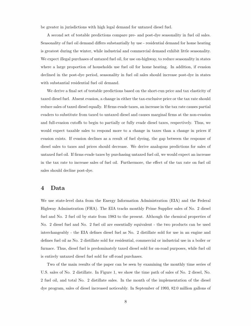
We derive a final set of testable predictions based on the short-run price and tax elasticity of
taxed diesel fuel. Absent evasion, a change in either the tax-exclusive price or the tax rate should
reduce sales of taxed diesel equally. If firms evade taxes, an increase in the tax rate causes partial
evaders to substitute from taxed to untaxed diesel and causes marginal firms at the non-evasion
and full-evasion cutoffs to begin to partially or fully evade diesel taxes, respectively. Thus, we
would expect taxable sales to respond more to a change in taxes than a change in prices if
evasion exists. If evasion declines as a result of fuel dyeing, the gap between the response of
diesel sales to taxes and prices should decrease. We derive analogous predictions for sales of
untaxed fuel oil. If firms evade taxes by purchasing untaxed fuel oil, we would expect an increase
in the tax rate to increase sales of fuel oil. Furthermore, the effect of the tax rate on fuel oil
sales should decline post-dye.
4 Data
We use state-level data from the Energy Information Administration (EIA) and the Federal
Highway Adminstration (FHA). The EIA tracks monthly Prime Supplier sales of No. 2 diesel
fuel and No. 2 fuel oil by state from 1983 to the present. Although the chemical properties of
No. 2 diesel fuel and No. 2 fuel oil are essentially equivalent - the two products can be used
interchangeably - the EIA defines diesel fuel as No. 2 distillate sold for use in an engine and
defines fuel oil as No. 2 distillate sold for residential, commercial or industrial use in a boiler or
furnace. Thus, diesel fuel is predominately taxed diesel sold for on-road purposes, while fuel oil
is entirely untaxed diesel fuel sold for off-road purchases.
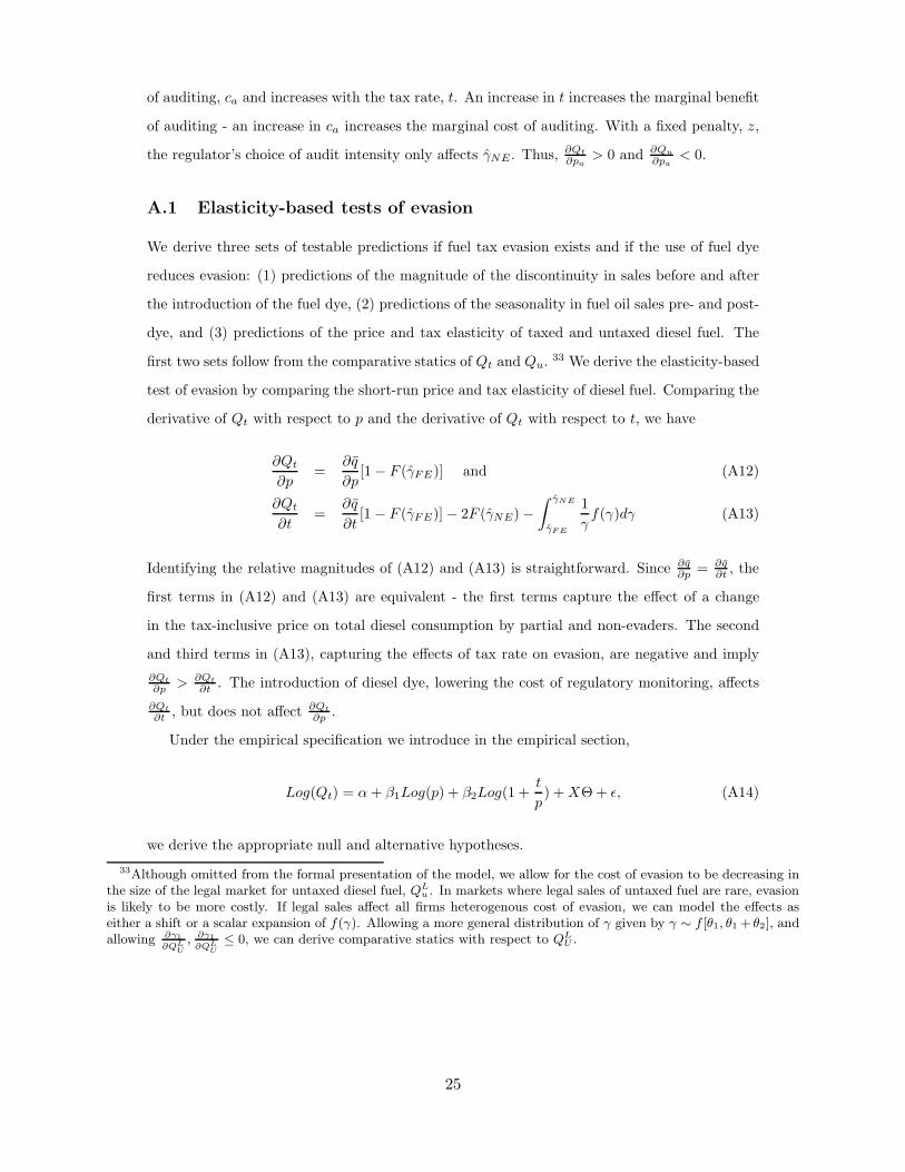
Two of the main results of the paper can be seen by examining the monthly time series of
U.S. sales of No. 2 distillate. In Figure 1, we show the time path of sales of No. 2 diesel, No.
2 fuel oil, and total No. 2 distillate sales. In the month of the implementation of the diesel
dye program, sales of diesel increased noticeably. In September of 1993, 82.0 million gallons of
8

diesel were sold per day in the United States, and this figure increased to 97.4 million gallons
per day in October of 1993. Sales of No. 2 fuel oil declined noticeably in the period after the dye
program was implemented, even though the discontinuity in the month of implementation is less
striking than with diesel due to the seasonality of fuel oil sales. Overall, the increase in diesel is
largely canceled out by the decrease in fuel oil sales, at least in the first year of implementation.
The EIA publishes the monthly average price of No. 2 distillate by type of end user for the
majority of states. When unavailable for a particular state, we utilize the price in the Petroleum
Administration for Defense District (PADD) in which the state is located. To measure the price
of diesel for on-road purposes, we use the price to end users through retail outlets. This is
virtually a perfect match of the low-sulfur diesel price, which is almost exclusively intended for
on-highway use in the post-dye period.
We obtain information about the federal and state on-road diesel tax rates from 1981 to 2003
from the Federal Highway Administration Annual Highway Statistics. Figure 2 plots the state
and federal tax rates over time. In Panel A, we show the federal tax in cents per gallon, which
was four cents per gallon in 1981, rising to the current level of 24.4 cents per gallon in 1993.
The only post-dye variation in the federal tax rate was a temporary 0.1 cent reduction in 1996.
In Panel B we plot the average state tax.15 The average state tax has increased monotonically
over time, starting at approximately 12 cents per gallon in 1983 and increasing to over 21 cents
per gallon in 2003. This figure also plots the number of states changing their tax rates in each
year. It is common for a state to change its tax rate - in most years, between 6 and 23 states
change diesel tax rates.16 Between-state variation also rises throughout the period. Figure 3
displays the distribution of state diesel tax rates separately for 1983, 1993, and 2003. In 1983,
state tax rates were concentrated between 10 and 15 cents per gallon, with all but seven states
having tax rates below 15 cents. During the course of the sample, diesel taxes grew and became
more disperse across states. By 2003, 26 percent of states had a diesel tax rate of at least 25
cents per gallon, higher than the federal rate of 24.4 cents per gallon.
To model legitimate demand for No. 2 fuel oil, we also capture demand factors, primarily
15Oregon does not tax diesel sold for trucking, instead taxing the number of weight-miles driven in the state. Forthis reason, we exclude Oregon from the subsequent analysis.
16The dye program eases tax collection, which creates an incentive to raise tax rates on diesel. Alt (1983), Kau andRubin (1981), and Balke and Gardner (1991) among others point to the importance of tax collection in shaping thetax structure. We do see the federal government raising tax rates in the period of the dye implementation, howeverwe do not observe a similar response by states, for whom the growth in the average tax rate actually falls post-dye.Political pressure may limit the ability to raise the tax rate. Furthermore, if states are simply trying to meet arevenue target, then the dye program may in fact place downward pressure on tax rates. Finally, the diesel tax isnot treated as general revenue for the states, but instead goes into its highway trust fund. This may limit the valueof extra revenue through this tax.
9

related to temperature and prevalence of the use of fuel oil as a home heating source. We obtain
data on monthly degree days by state from the National Climate Data Center at the National
Oceanic and Atmospheric Administration. The number of degree days in a month is often used
to model heating demand and is a measure of the amount by which temperatures fell below a
given level on a particular day, summed across the days of the month. We also measure state
heating oil prevalence from the 1990 census using the fraction of households in a state reporting
fuel oil as the primary energy source used for home heating.
Finally, we instrument for diesel prices using the Brent crude oil spot price and event dummy
variables corresponding to the first and second Iraq wars and the 2002 Venezuelan oil strike.
Brent crude is a globally-priced commodity commonly used as an instrument for regional product
prices.17 The validity of this instrument depends on the extent to which demand shocks for US
diesel are incorporated into world oil prices. This effect is likely to be small given that US diesel
demand accounted for approximately 4.6% of world crude production in 1993 and 4.9% of world
crude production in 2005. 18
Table 1 displays summary statistics of the data. In the first two rows we show the pre- and
post- means for the two primary variables of interest - No. 2 diesel, which is largely used for
taxed purposes, and No. 2 fuel oil, which is reported to be used for entirely untaxed purposes.19
The average state-month in the pre-dye period saw 1.4 million gallons of diesel sold per day,
slightly greater than the 1.3 million gallons of fuel oil sold per day. This difference grows
considerably in the post-period, when diesel sales rise to 2.3 million gallons per day while fuel
oil sales fall to 0.8 million gallons per day.
The average tax in the pre-dye period represents a significant fraction of the purchase price
in the typical state. In the pre-dye period, the average state plus federal tax is 30.5 cents per
gallon, compared with a tax excluded price of 77.8 cents per gallon for purchasers of diesel
through retail outlets. This represents 28 percent of the final purchase price. Taxes are growing
over time, representing 35 percent of the purchase price in the post-period. The price of sales
to residential users, which is likely to represent sales of home heating oil, is higher than the tax
17For example, Borenstein and Shepard (2002) use the Brent crude spot price to form an instrument for US crudefutures prices on the New York Mercantile Exchange. In addition, Asche, Gjolberg and Volker (2003) find the Brentcrude price is exogenous to regional European petroleum product shocks.
18In 1993, world crude production was 24.7 billion barrels of which approximately 1.15 billion barrels were consumedas distillate in the United States. In 2005, world crude production was 30.8 billion barrels, of which 1.5 billion barrelswere consumed domestically as distillate oil.
19Reported diesel sales also include agricultural uses. The importance of agriculture in reported diesel sales can beassessed by examining low-sulfur versus high-sulfur diesel sales. After the low-sulfur regulations went into effect foron-highway sales, diesel sales were reported separately for low- and high-sulfur. The former is entirely on-highwaypurchases. In the post-dye period, the average state had 2316 gallons per day of diesel sales in the average month,2005 of which was low-sulfur, indicating that untaxed uses represent less than 15 percent of reported diesel sales.
10

excluded retail price of No. 2 distillate, likely due to the incorporation of delivery costs.
Table 1 also reports the average sales of other distillates.20 No. 2 distillate is far more
important than the other distillates. In the pre-dye period, 67 thousand gallons of No. 1
distillate and 133 thousand gallons of No. 4 distillate are sold.
Missing values are common in the EIA quantity series. In months where few suppliers are
serving a particular state, the quantity value is suppressed by the EIA if it is possible to infer
the sales from a particular firm. For diesel, 9 percent of observations are missing in the pre-dye
period compared to 20 percent in the post-dye period. In the case of fuel oil, missing values
represent 10 and 24 percent of the state-months in the pre- and post-dye periods, respectively.
Although we estimate our results off of the non-missing observations, the results change little
when we instead interpolate the missing values using state specific time trends.
5 Dye Program and Diesel Misreporting
In this section we examine the response of No. 2 diesel and No. 2 fuel oil sales to the diesel dye
program. The main effect of the program was to substantially reduce the cost of monitoring
firm tax compliance. Our model predicts that as the cost of monitoring declines, enforcement
rises and firms comply more fully, reporting more taxed purchases and fewer untaxed purchases.
Since evasion here simply involves mislabeling the use of No. 2 distillate, there should be no
adjustment costs in production and therefore the primary effect of the dye program on quantities
should be seen immediately.21
To evaluate the response of reported taxed and untaxed sales of No. 2 distillate, we estimate
a specification of the break in trend of log quantity of the form
lnqit = β0 + δ1postdyet + ΠXit + f(t) + ρi + εit (1)
where lnqit is the log of the quantity of diesel or fuel oil sold in state i in month t, Xit is a
vector of state-month covariates, and ρi represents a state fixed effect. The function f(t) reflects
overall time trends in the demand for gallons, which we parameterize using a flexible quadratic
polynomial whose slope is allowed to vary in the pre- and post-dye periods.
20These are outputs of the distillation process of crude oil, however are in general not substitutable with No. 2distillate. Some outputs can be blended with No. 2 diesel to lower the sulfur content or the tax per unit, though thisis only possible to a very limited extent.
21It is possible that some adjustment may occur over time if firms learn about the effect of the program on thelikelihood of getting caught, or if detecting evaders becomes easier as fewer firms evade. While plausible, thesemechanisms are difficult to distinguish empirically from unrelated shifts in demand for diesel over time. In addition,anticipation of the dye program would conservatively bias our results.
11

Table 2 displays the results from estimating (1). In column 1, we show the estimated
discontinuity in diesel sales controlling only for the quadratic time trend. Sales of No. 2 diesel
rose by an estimated 29 percent upon dye implementation. Panel A of Figure 4 shows the
fit of the quadratic time trend to average actual log diesel sales. The quadratic time trend
seems highly successful at fitting the time profile of diesel sales. In the specification shown in
column 2 of Table 2, we include state effects and other state-month covariates and find that
the estimated discontinuity is stable when adding these controls. In the full specification, the
estimated discontinuity in diesel is 26 percent.
Counteracting the increase in diesel sales is a decrease in the sales of fuel oil. Columns 3-4 of
Table 2 display estimates of the discontinuity of fuel oil sales. We estimate that the average state
experienced a 31 percent decrease in fuel oil sales, controlling only for the quadratic time trend.
Again the estimated coefficient is fairly stable when adding covariates. In the full specification,
we estimate a 39 percent decrease in fuel oil sales due to the dyeing program. As with diesel fuel,
the quadratic time trend is successful at capturing the time path of fuel oil sales, as evidenced
by Panel B of Figure 4.
Based on the significant increase in diesel sales and corresponding decrease in fuel oil sales,
we conclude that there is evidence of a significant response of taxed and untaxed sales to the
dye program. Columns 5-6 of Table 2 display the results of a similar specification for fuel oil’s
share of No. 2 distillate. This specification is desirable as it provides a sense of the importance
of the substitution between diesel and fuel oil as a share of all No. 2 distillate, and it provides
for a more direct comparison with the evasion parameter α from the model. Fuel oil’s share
of distillate fell by 11 percent when the dye program was implemented, and this estimated
discontinuity changes little when additional covariates are included. In the full specification, we
estimate a discontinuity of 12.5 percent in the average state’s share of No. 2 distillate.
While the log specification allows one to easily assess the magnitude of the discontinuity in
percentage terms, a drawback is that it does not allow for a direct evaluation of the substitution
between diesel and fuel oil. The model presented in Section 3 suggests that this substitution
will be on a one-for-one basis, however this cannot be evaluated in the log specification due
to the different levels of diesel and fuel oil.22 While the log specification will be preferred in
estimating demand elasticities, to more directly evaluate the substitution between diesel and
fuel oil we estimate (1) using the level of sales as the dependent variable. To account for the
22The result of one-for-one substitution in the model will not literally be true if the size of the penalty depends onthe degree of evasion. In this case, altering the likelihood of getting caught changes the marginal purchase decision forthe remaining full evaders, so that they reduce purchases of the untaxed quantity without a corresponding increasein their reported purchases of taxed diesel.
12

difference in levels across states, we form per capita sales by normalizing quantities by yearly
state population.
Table 3 presents the results. In the full specification, diesel sales increased by 0.067 gallons
per person per day in the post-dye period, which is matched by a 0.066 gallons per person
decline in fuel oil sales. In columns 5-6 we examine the break in the sales of all No. 2 distillate,
the sum of diesel and fuel oil sales. We estimate an increase of 0.005 increase in No. 2 distillate
sales post-dye, which is both statistically and economically insignificant. These results together
suggests a one-for-one substitution between fuel oil and diesel post-dye.
We next investigate the extent to which the break in diesel and fuel oil sales is correlated with
factors that alter ex ante evasion incentives. First, we estimate the break in trend separately
for states with many legitimate uses for untaxed No. 2 distillate. In these states, evaders may
find it easier to acquire the untaxed alternative, and it will likely be more difficult for auditors
to detect illegitimate users. Second, we estimate the trend break separately for states with high
tax rates versus states with low tax rates. According to the model, states with higher tax rates
should experience greater evasion, and therefore should see a larger increase in taxed diesel at
the dye implementation date.
Panel A of Table 4 shows the results for per capita diesel sales. Column 1 repeats the base
specification for the full sample. We first split the sample by the prevalence of heating oil use for
home heating as reported in the 1990 census. Consistent with our hypothesis, the dye response
is heavily concentrated in high heating oil states. These states experienced an increase in diesel
sales of 0.09 gallons per person per day, compared with an increase of 0.04 gallons in states with
a low prevalence of home heating oil. 23
We next split the sample between low and high diesel tax states, as measured by states’
tax rates in December of 1992, prior to the announcement of the dye program. The estimated
break in the diesel series is larger in states with high tax rates, with an estimated break of 0.077
gallons per person per day. The increase is 0.059 gallons in low tax states.
Panel B of Table 4 shows the results of similar specifications for per capita fuel oil use.
Similar to the diesel results, fuel oil sales fell by more in states with high heating oil use by
households, where sales were 0.079 gallons per person per day lower post-dye, compared to
low-heating oil states, where sales were lower by 0.055 gallons. Unlike with diesel, however, the
23Agricultural use also represents a sizable block of legitimate users, and a similar test could be performed bysplitting states based on the importance of agriculture in state GSP. However, our measure of diesel includes untaxedagricultural uses, which makes such a test less informative than examining high versus low heating oil states. In fact,we find that the break in trend is in fact somewhat larger in low agriculture states, though interestingly we find theopposite result when considering fuel oil’s share of No. 2 distillate.
13

estimated decline in fuel oil sales is similar for high- versus low-tax states.
In Panel C, we present evidence regarding the response of fuel oil’s share of number 2 distillate
to the dye program, which will summarize the substitution between diesel and fuel oil post-dye.
For all states, fuel oil’s share of distillate fell by 12.6 percentage points. This decline was greater
in high fuel oil states, where fuel oil’s share fell by 14.7 percentage points, and in states with
high tax rates, where the decline was 14.3 percentage points.
Finally, we provide additional evidence that a greater portion of fuel oil sales were legiti-
mate post-dye, by examining the seasonality in fuel oil sales in the pre- and post-dye period.
Seasonality varies by state, depending on the nature of fuel oil demand. Residential demand
for fuel oil peaks strongly during the winter. Industrial and commercial demand for fuel oil is
slightly higher during the summer, largely from greater use of fuel oil for electric generation.
Thus, northern states with a high proportion of households using fuel oil for home heating tend
to have much higher demand during the winter than the summer, while states with insignificant
residential demand tend have slightly higher sales during the summer. Based on our estimates
that at least 30-40 percent of fuel oil purchases in the pre-dye period were illegally used for
on-highway purposes, we expect fuel oil sales in the pre-dye period to exhibit less seasonality,
particularly in states with a high proportion of households using fuel oil for home heating.
In Table 5, we present estimates of the seasonality of fuel oil demand pre- and post-dye. In
the first specification, we regress log fuel oil sales on the number of degree days in a particular
state-month, the number of degree days interacted with the fraction of households in the state
who reported using heating oil as the primary home heating fuel in the 1990 census, sets of
pre- and post- state fixed effects and a pre- and post- quadratic time trend. To estimate the
change in seasonality, we interact the first two explanatory variables with a post-dye dummy
variable. Specifications (2) and (3) include state-invariant and state-specific month fixed effects,
respectively.
In the first two specifications, we estimate a small, but significant, negative coefficient on
degree days and a large, positive and significant coefficient on the interaction between degree
days and the fraction of homes using fuel oil. States with substantial residential demand peak
strongly during the winter, while states with little residential demand peak slightly during the
summer. When we control for state-specific seasonality by including state-specific month fixed
effects, we find that both the pre-dye coefficients are positive. Controlling for state-specific
seasonality, atypically cold months are associated with increased fuel oil demand - the effect is
pronounced in states with high proportion of residences using fuel oil for home heating. Across
14

all three specifications, we find that the post-dye, degree day, home heating interaction term is
positive and significant - consistent with an increase in seasonality post-dye in states with high
demand for home heating oil.
6 Evasion estimation using elasticities
In this section, we empirically apply three aspects of the model described in Section 3. First,
we test for evasion in the pre-dye and post-dye periods by estimating separate price and tax
elasticities. Second, we use these estimated coefficients to obtain estimates of the gradient of
evasion with respect to taxes. Finally, we describe how evasion’s response to the tax rate alters
the revenue effects of increasing the diesel tax. The advantage of each of these applications is
that they require only observing taxed gallons, and as a consequence, could be broadly applied
outside of the context of diesel fuel. In the current application, we are able to observe the
primary untaxed alternative, which we can use to support the validity of our estimates of the
evasion-tax gradient.
6.1 Testing for evasion
As shown in the appendix, we can separately identify the tax and price elasticities by factoring
price out of ln(p + t). We will estimate a version of (1) for diesel fuel that includes the log of
the price and the log of (1 + t/p) as separate regressors:
lnqit = β0 + β1ln(pit) + β2ln(1 + τit/pit) + ΠXit + f(t) + αi + εit. (2)
We estimate the model using the Brent crude spot price and our dummy variables corresponding
to the first and second Iraq Wars and the 2002 Venezuelan Oil Strike as instruments for ln(pit)
and ln(1 + τit/pit).
Absent evasion, demand for taxed diesel should respond equally to a change in taxes and
prices.24 As we derive in the appendix, the appropriate null hypothesis to test for the presence of
evasion equates β1 and β2 - finding that β1 is significantly greater than β2 is consistent with the
presence of evasion. Since our discontinuity results suggest that the dye program significantly
24One caveat is if firms or consumers view changes in pre-tax prices to be transitory and changes in tax rates to bepermanent, in which case these two elasticities could differ. First, if changing demand involves an adjustment cost,the response to a transitory price shock will be lower. Alternatively, if firms can substitute purchases over time, theresponse to transitory price shocks will be greater. However, we will show that the post-dye elasticities are the same,and that the timing of the narrowing of the difference between these elasticities matches with the implementation ofthe dye program. The aforementioned bias is unlikely to explain these two patterns.
15
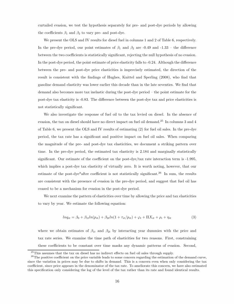
curtailed evasion, we test the hypothesis separately for pre- and post-dye periods by allowing
the coefficients β1 and β2 to vary pre- and post-dye.
We present the OLS and IV results for diesel fuel in columns 1 and 2 of Table 6, respectively.
In the pre-dye period, our point estimates of β1 and β2 are -0.49 and -1.33 – the difference
between the two coefficients is statistically significant, rejecting the null hypothesis of no evasion.
In the post-dye period, the point estimate of price elasticity falls to -0.24. Although the difference
between the pre- and post-dye price elasticities is imprecisely estimated, the direction of the
result is consistent with the findings of Hughes, Knittel and Sperling (2008), who find that
gasoline demand elasticity was lower earlier this decade than in the late seventies. We find that
demand also becomes more tax inelastic during the post-dye period – the point estimate for the
post-dye tax elasticity is -0.83. The difference between the post-dye tax and price elasticities is
not statistically significant.
We also investigate the response of fuel oil to the tax levied on diesel. In the absence of
evasion, the tax on diesel should have no direct impact on fuel oil demand.25 In columns 3 and 4
of Table 6, we present the OLS and IV results of estimating (2) for fuel oil sales. In the pre-dye
period, the tax rate has a significant and positive impact on fuel oil sales. When comparing
the magnitude of the pre- and post-dye tax elasticities, we document a striking pattern over
time. In the pre-dye period, the estimated tax elasticity is 2.184 and marginally statistically
significant. Our estimate of the coefficient on the post-dye/tax rate interaction term is -1.995,
which implies a post-dye tax elasticity of virtually zero. It is worth noting, however, that our
estimate of the post-dye*after coefficient is not statistically significant.26 In sum, the results
are consistent with the presence of evasion in the pre-dye period, and suggest that fuel oil has
ceased to be a mechanism for evasion in the post-dye period.
We next examine the pattern of elasticities over time by allowing the price and tax elasticities
to vary by year. We estimate the following equation:
lnqit = β0 + β1tln(pit) + β2tln(1 + τit/pit) + ϕt + ΠXit + ρi + ηit (3)
where we obtain estimates of β1t and β2t by interacting year dummies with the price and
tax rate series. We examine the time path of elasticities for two reasons. First, constraining
these coefficients to be constant over time masks any dynamic patterns of evasion. Second,
25This assumes that the tax on diesel has no indirect effects on fuel oil sales through supply.26The positive coefficient on the price variable leads to some concern regarding the estimation of the demand curve,
since the variation in prices may be due to shifts in demand. This is a concern even when only considering the taxcoefficient, since price appears in the denominator of the tax rate. To ameliorate this concern, we have also estimatedthis specification only considering the log of the level of the tax rather than its rate and found identical results.
16

exploiting the timing of changes in the estimated elasticities ameliorates concerns regarding
bias in the demand estimation. Our estimates of the price and tax elasticities could be biased
since variation in price could reflect shifts in demand and therefore movements along the supply
curve. Estimating the elasticities by year allows us to examine the timing of the shift in the tax
elasticity relative to the price elasticity. While estimates of the gap between these two may be
biased, there is little reason for shifts in this gap to coincide with the timing of the dye program
aside from a reduction in evasion.
In Figure 5, we plot the yearly estimates of β1 and β2 for log diesel sales. In the pre-dye
period, there is a consistent gap between the estimated tax and price elasticities. Over time,
demand appears to become less price sensitive. In the years immediately following the dye
program’s implementation, the gap between the tax and price elasticities is virtually zero, sug-
gesting that the addition of dye may have significantly curbed diesel tax evasion. An interesting
pattern emerges in the latter portion of the sample. During this time, the gap between the tax
and price elasticities reappears. This may point toward a dynamic response of evaders, who
may have developed new evasion technologies in response to the dye program.
As further evidence that the timing of the tax responsiveness coincided with the dye program,
we examine the time path of the elasticity of fuel oil with respect to the diesel tax rate. In Figure
6, we plot the estimated yearly fuel oil tax rate elasticity. For almost every year prior to 1993,
we estimate a positive tax elasticity. In 1993, this elasticity drops to close to zero. Unlike our
estimates for diesel fuel, the responsiveness of fuel oil to the tax rate does not seem to reappear.
This suggests that any new evasion methods did not involve fuel oil.
6.2 Evasion response to tax
A parameter of significant interest in the public finance literature is the responsiveness of evasion
to the tax rate. In the previous section, we arrived at a reasonable pre-dye estimate for this
measure by examining the response of fuel oil to the tax rate, as this seems to be a primary
mechanism for evading the diesel tax. In most settings, observing evasion directly is not possible.
In addition to suggesting a test for evasion using estimates of the price and tax elasticities, our
model also demonstrates how the coefficients for β1 and β2 can be used to obtain an estimate
of the degree to which evasion responds to the tax rate.
As derived in the appendix, we can express the derivative of evasion with respect to taxes
17

as a function of the coefficients β1 and β2 from equation (2).
∂E
∂t=
Qt
p[β1 − β2]. (4)
Importantly, this metric of evasion only depends on information about taxed sales, which are
typically observable. In fact, the case of fuel tax evasion provides an unusual example in which
untaxed sales are also available, and we use this extra information to evaluate the performance
of our evasion estimate. From (4), we can obtain an estimate of the derivative of evasion with
respect to taxes. We obtain average values for Qt and p from Table 1 and the coefficients β1 and
β2 from the first column of Table 6. In the pre-dye period, we estimate that each cent increase
in the tax rate increased the quantity of unreported gallons by 16.5 thousand per day. In the
post-dye period, this falls modestly to 15.4 thousand gallons per day. These values represent
1.1 percent and 0.7 percent of the average level of taxed diesel sold per day, respectively.
While these estimates rely solely on observing taxed gallons, we can assess their validity
by comparing them to the pre-dye response of fuel oil to tax changes. From (2), we use the
parameter estimate β2 to obtain ∂Qu
∂t = Qu
p+tβ2. Plugging in for the average price, tax, and
untaxed quantity in the pre-dye period, and using the estimate of β2 from the third column of
Table 6, we find that increasing taxes by one cent increased purchases of fuel oil by 25.2 thousand
gallons per day. This estimate is slightly larger than that obtained from taxed gallons, indicating
that the latter may represent a conservative estimate of the evasion-tax gradient.
6.3 Evasion and tax revenues
Ideally we would like to state the response of evasion to taxes as an elasticity, though in a setting
where the level of untaxed gallons is unobserved this is not possible. To put the evasion-tax
gradient into perspective, we instead examine how tax revenues respond to changes in the tax
rate, and how this is altered by tax evasion. The elasticity of revenue with respect to the tax
rate captures the change in tax revenues arising from both the decreased consumption of taxed
diesel fuel by compliant firms and substitution from legal to illegal purchases by non-compliant
firms. These two effects are captured in equation (A21), restated here:
∂tQt
∂t
t
tQt= 1 +
t
t + pβ1 − t
t + p(β1 − β2). (5)
The term involving only β1 captures the traditional behavioral response, while the final term
reflects the effect of evasion. In the absence of evasion, β1 and β2 are identical, leading the
18

latter term to disappear. We can therefore use our estimates of the price elasticity β1 to obtain
an estimate of the revenue effects of changing taxes if evasion were not present. In the pre-dye
period, this implies an elasticity of revenue with respect to the tax rate of 0.85, and in the
post-dye period this increases to 0.90. The erosion of the tax base due to greater evasion when
taxes are increased, as documented in section 6.2, has a significant impact on the fraction of
tax increases that are incorporated into revenues. Allowing for evasion, and therefore for the
differing values of β1 and β2, we find a revenue-tax elasticity of 0.60 in the pre-dye period and
0.71 in the post-dye period. A tax increase in the dye regime translates into 11 percent higher
revenues than in the pre-dye period. Based on the estimates absent evasion, the lower price
sensitivity post-dye can account for less than half of this.
7 Conclusion
This paper considers the evasion of diesel taxes, and how this evasion responds to the large shift
in the cost of conducting an audit represented by the addition of red dye to untaxed diesel. The
setting we consider provides a unique opportunity to observe both a taxed commodity as well as
an untaxed substitute. We find that reducing the cost of audit greatly improves tax compliance,
and that diesel tax evasion responds positively to tax rates. The estimated responses of diesel
and fuel oil to the dyeing program are strikingly similar, as there are significant discontinuities
in the sales of No. 2 diesel and No. 2 fuel oil, yet little change in overall No. 2 distillate sales.
While the current application has the luxury of observing the evasion vehicle, untaxed fuel
oil, it is often the case that only taxed quantities are observed. We apply a simple method for
detecting the evasion of specific quantity taxes from the observed taxed quantities, and show
how this method can be used to estimate the response of evasion to the tax rate. Finally, we
use these measures to describe how evasion affects the tax revenue response to tax increases, a
parameter of considerable interest in public economics.
The reduction in evasion we document post-dye has potentially large welfare consequences.
Resources spent evading taxes represent a pure deadweight loss. The additional tax revenue
resulting from compliance efforts represents a first-order approximation of the welfare gain. If
firms evade taxes until the marginal cost of evasion equals the tax rate, then the tax rate informs
as to the deadweight loss associated with the marginal gallon of unreported taxable diesel, and
we can estimate the welfare gain by multiplying the tax rate by the change in taxed gallons.
The average state plus federal diesel tax rate in 1993 was 39 cents per gallon. We estimate that
19
taxed diesel sales rose by approximately 26 percent post-dye, or 7.1 billion gallons per year.27
A first-order approximation of the welfare gain is therefore $2.8 billion per year.
This should represent an upper bound of the welfare gain for several reasons. First, as
Chetty (2008) notes, if the penalty of being caught affects the marginal evasion decision, then
the marginal cost of evasion will be less than the tax rate. Second, the marginal cost of evasion
is likely to be increasing in evasion, which would imply that the average cost of evasion is
lower than the marginal cost of evasion. Finally, the extent of fully evading firms will alter
this calculation, as the marginal cost of evasion will be less than the tax rate for these firms
and because the enforcement efforts will reduce their supply. Nonetheless, the improvement in
efficiency is likely to be large.
Given the large efficiency and revenue gains, it is worth asking if the current level of invest-
ment in enforcement technologies is optimal. For instance, Baluch (1996) estimates that taxes
assessed as a direct result of enforcement activity are 10 to 18 times greater than the cost of
the enforcement activity. However, it is unclear what this tells us regarding the optimal level
of enforcement, since we have little idea regarding the marginal return to enforcement efforts
even if we have good estimates of the average return. Still, there are reasons to believe the cur-
rent level of enforcement does not maximize revenue. For instance, both states and the federal
government collect taxes, and the enforcement efforts of one generates a positive externality on
the collections of the other. Furthermore, governments may have an objective function where
revenue is not the primary argument.
27The average diesel sales were 75 million gallons per day in the 12 months prior to the dye program.
20

References
[1] Allingham, Michael G. and Agnar Sandmo. (1972) “Income Tax Evasion: A TheoreticalAnalysis,” Journal of Public Economics 1:3-4, p. 323-338.
[2] Alt, James. (1983) “The Evolution of Tax Structures,” Public Choice 41:1, p. 181-222.
[3] Alm, James and Michael McKee. (2005) “Audit Certainty and Taxpayer Compliance,”Working paper, Georgia State University.
[4] Asche, Frank, Ole Gjolberg, and Teresa Volker (2003) “Price relationships in the petroleummarket: an analysis of crude oil and refined product prices,” Energy Economics 25, p. 289-301.
[5] Balke, Nathan S. and Grant W. Gardner. (1991) “Tax Collection Costs and the Size ofGovernment,” Working paper, Southern Methodist University.
[6] Baluch, Stephen (1996) Revenue Enhancement Through Increased Motor Fuel Tax En-forcement. Transportation Research Record 1558
[7] Beron, Kurt J., Helen V. Tauchen, and Ann Dryden Witte. (1992) “The Effect of Auditsand Socioeconomic Variables on Compliance,” in Why People Pay Taxes, edited by JoelSlemrod. Ann Arbor: University of Michigan Press.
[8] Borenstein, S. and A. Shepard (2002), “Sticky Prices, Inventories and Market Power inWholesale Gasoline Markets.” Rand Journal of Economics, 33 (1), pp. 116-139.
[9] Chetty, Raj. (2008) “Is the Taxable Income Elasticity Sufficient to Calculate DeadweightLoss? The Implications of Evasion and Avoidance,” working paper.
[10] Chetty, Raj, Adam Looney and Kory Kroft. (2007) “Salience and Taxation: Theory andEvidence from a Field Experiment,” working paper.
[11] Clotfelter, Charles T. (1983) “Tax Evasion and Tax Rates: An Analysis of IndividualReturns,” Review of Economics and Statistics 65:3, p. 363-373.
[12] DellaVigna, Stefano and Eliana La Ferrara. (2006) “Detecting Illegal Arms Trade,” workingpaper.
[13] Denison, Dwight V., and Robert J. Eger. (2000) “Tax Evasion from the Policy Perspective:The Case of the Motor Fuel Tax ,” Public Administration Review 60:2, 163-172.
[14] Dubin, Jeffrey A. and Louis L. Wilde. (1988) “The Empirical Analysis of Federal IncomeTax Auditing and Compliance,” National Tax Journal 41:1, 61-74.
[15] Feinstein, Jonathan. (1991) “An Econometric Analysis of Income Tax Evasion and itsDetection,” RAND Journal of Economics 22:1, p. 14-35.
[16] Feige, Edgar L. (1979) “How Big is the Irregular Economy?” Challenge 22:5, p. 5-13.
[17] Fisman, Raymond and Shang-Jin Wei. (2004) “Tax Rates and Tax Evasion: Evidence from“Missing Imports” in China,” Journal of Political Economy 112:2, p. 471-496.
[18] Gutmann, Peter M. (1977) “The Subtarranean Economy,” Financial Analysts Journal 33:6,p. 26-34.
[19] Hsieh, Chang-Tai and Enrico Moretti. (2006) “Did Iraq Cheat the United Nations? Un-derpricing, Bribes, and the Oil for Food Program,” The Quarterly Journal of Economics121:4, p. 1211-1248.
[20] Hughes, Jonathan E., Christopher R. Knittel, and Daniel Sperling. (2008) “Evidence of aShift in the Short-Run Price Elasticity of Gasoline Demand,” The Energy Journal 29:1.
[21] Kau, James B. and Paul H. Rubin. (1981) “The Size of Government,” Public Choice 37:2,p. 261-274.
[22] Pommerehne, Werner W. and Hannelore Weck-Hannemann. (1996) “Tax rates, tax admin-istration and income tax evasion in Switzerland,” Public Choice 88, p. 161-170.
21

[23] Rosen, Harvey. (1976) “Tax Illusion and the Labor Supply of Married Women,” The Reviewof Economics and Statistics 58:2, p. 167-172.
[24] Slemrod, Joel, Martha Blumenthal, and Charles Christian (2001) “Taxpayer response toan increased probability of audit: evidence from a controlled experiment in Minnesota,”Journal of Public Economics 79, p. 455-483.
[25] Wenzel, Michael and Natalie Taylor. (2004) “An experimental evaluation of tax-reportingschedules: a case of evidence-based tax administration,” Journal of Public Economics 88,p. 2785-2799.
[26] Yitzhaki, Shlomo. (1974) “A Note on ‘Income Tax Evasion: A Theoretical Analysis,’”Journal of Public Economics 3, p. 201-202.
22

A Appendix
We consider a model of evasion in which a continuum of firms purchase diesel for on-road (taxed)
used. Firms choose a quantity of diesel fuel q to produce output x(q) and the percent of untaxed
(illegal) fuel, α. Normalizing the price of output to 1, firms purchase taxed diesel fuel at price
p + t and untaxed diesel fuel at price p. Firms vary in their cost of evasion - a firm located
at γ ∼ f [0, θ] choosing to evade incurs a heterogeneous cost of evasion, ce(qu, γ) = γ(αq)2/2.
In addition to paying the cost of evasion, firms are penalized if caught evading taxes by the
regulator. The regulator deters tax evasion by randomly auditing firms with an endogenous
probability pa and assessing a fixed penalty, z, if qu > 0.28
First, the regulator observes z, f(γ), ca, p and t and credibly commits to auditing firms with
probability, pa. 29 The regulator chooses pa to maximize tax revenues less enforcement costs,
given by
W = tQt − cap2
a
2, (A1)
where Qt is the total purchases of the taxed diesel.30 After the regulator chooses pa, each
risk-neutral firm chooses q and α, conditional on γ, to maximize expected profits given by
E[Π] = x(q) − (pαq + γ(αq)2
2) − (p + t)(1 − α)q − pazI(α > 0) (A2)
subject to
q ≥ 0, α ∈ [0, 1]. (A3)
Let q denote the quantity of diesel fuel satisfying (??) for interior solutions of α, given by
x′(q) = p + t. (A4)
The threshold values for gamma separating full evaders(α∗ = 1), partial evaders (α∗ ∈ (0, 1))
and non-evaders(α∗ = 0) are defined by setting (??) equal to 1, and equating E[Π|α = tqγ ] and
28The fixed component of the penalty is a sufficient condition for the existence of entirely legal firms, so long asθ, the upper bound on the cost of evasion parameter, is sufficiently high. Our testable implications do not changeif we generalizing the penalty function to allow for the penalty to vary linearly with the amount of untaxed dieselpurchased.
29We treat z as exogenously given. If the regulator can choose both pa and z, the optimal decision for the regulatoris to set extremely high penalties and low enforcement.
30We present the model in which fines do not enter into the regulator’s objective function. The comparative staticresults do not substantively change with this inclusion or exclusion of the fines.
23
E[Π|α = 0].
γ̂FE = t/q (A5)
γ̂NE =t2
2paz. (A6)
Conditional on pa, the optimal choices of q∗(γ|pa) and α∗(γ|pa) are given by
q∗(γ|pa) =
⎧⎪⎪⎪⎨⎪⎪⎪⎩
x′(q) = p + γq for γ ∈ [0, t/q]
q for γ ∈ (t/q, t2
2paz )
q for γ ∈ [ t2
2paz , θ],
(A7)
and
α∗(γ|pa) =
⎧⎪⎪⎪⎨⎪⎪⎪⎩
1 for γ ∈ [0, t/q]
tqγ for γ ∈ (t/q, t2
2paz )
0 for γ ∈ [ t2
2paz , θ].
(A8)
Diagram 1 graphically represents how taxed and untaxed diesel consumption vary with the
evasion cost parameter, γ.
Aggregate consumption of taxed diesel, Qt, and untaxed diesel, Qu, are given by
Qt =∫ t2
2paz
t/q
q(1 − α)f(γ)dγ + (1 − F (t2
2paz))q and (A9)
Qu =∫ t/q
0
q∗(γ)f(γ)dγ +∫ t2
2paz
t/q
qαf(γ)dγ. (A10)
Substituting (A9) into the objective function, the solution to regulator enforcement problem
solves the first-order condition
pa =
√t2
caf(γ̂NE). (A11)
Unlike the firm problem which, conditional on pa, is independent of the distribution of γ, the
regulator’s choice of p∗a depends on the distribution of γ. Since γ̂NE is itself a function of pa,
more than one value of pa may solve the first order condition.31 In the event that more than
one local solution to the first order condition exists, the regulator selects the solution for which
the objective function is maximized.32 The intensity of enforcement, pa, decreases with the cost
31If the distribution of γ has a finite upper bound, note that a trivial solution to the first order condition is givenby pa = 0. In the context of diesel fuel tax enforcement, we focus on interior solutions for pa consistent with regulatorrevealed preference.
32A sufficient condition for a unique non-zero solution is f(γ) weakly monotonically increasing in γ. The sufficientcondition, that there are weakly more consumers with higher costs of evasion than lower costs of evasion, is reasonablein the context of diesel fuel tax evasion.
24
of auditing, ca and increases with the tax rate, t. An increase in t increases the marginal benefit
of auditing - an increase in ca increases the marginal cost of auditing. With a fixed penalty, z,
the regulator’s choice of audit intensity only affects γ̂NE . Thus, ∂Qt
∂pa> 0 and ∂Qu
∂pa< 0.
A.1 Elasticity-based tests of evasion
We derive three sets of testable predictions if fuel tax evasion exists and if the use of fuel dye
reduces evasion: (1) predictions of the magnitude of the discontinuity in sales before and after
the introduction of the fuel dye, (2) predictions of the seasonality in fuel oil sales pre- and post-
dye, and (3) predictions of the price and tax elasticity of taxed and untaxed diesel fuel. The
first two sets follow from the comparative statics of Qt and Qu. 33 We derive the elasticity-based
test of evasion by comparing the short-run price and tax elasticity of diesel fuel. Comparing the
derivative of Qt with respect to p and the derivative of Qt with respect to t, we have
∂Qt
∂p=
∂q̄
∂p[1 − F (γ̂FE)] and (A12)
∂Qt
∂t=
∂q̄
∂t[1 − F (γ̂FE)] − 2F (γ̂NE) −
∫ γ̂NE
γ̂F E
1γ
f(γ)dγ (A13)
Identifying the relative magnitudes of (A12) and (A13) is straightforward. Since ∂q̄∂p = ∂q̄
∂t , the
first terms in (A12) and (A13) are equivalent - the first terms capture the effect of a change
in the tax-inclusive price on total diesel consumption by partial and non-evaders. The second
and third terms in (A13), capturing the effects of tax rate on evasion, are negative and imply∂Qt
∂p > ∂Qt
∂t . The introduction of diesel dye, lowering the cost of regulatory monitoring, affects∂Qt
∂t , but does not affect ∂Qt
∂p .
Under the empirical specification we introduce in the empirical section,
Log(Qt) = α + β1Log(p) + β2Log(1 +t
p) + XΘ + ε, (A14)
we derive the appropriate null and alternative hypotheses.
33Although omitted from the formal presentation of the model, we allow for the cost of evasion to be decreasing inthe size of the legal market for untaxed diesel fuel, QL
u . In markets where legal sales of untaxed fuel are rare, evasionis likely to be more costly. If legal sales affect all firms heterogenous cost of evasion, we can model the effects aseither a shift or a scalar expansion of f(γ). Allowing a more general distribution of γ given by γ ∼ f [θ1, θ1 + θ2], andallowing ∂γ1
∂QLU
, ∂γ1∂QL
U
≤ 0, we can derive comparative statics with respect to QLU .
25

Taking derivatives with respect to p and t, we have
1Qt
∂Qt
∂p=
1p(β1 − β2
t
p + t) (A15)
1Qt
∂Qt
∂t= β2(
1p + t
) (A16)
Absent evasion34, we would expect a unit change in price and a unit change in consumer tax
incidence to have the same effect on taxed diesel sales. Thus,
1Qt
∂Qt
∂p=
1Qt
∂Qt
∂t→ H0 : β1 = β2. (A17)
A.2 Estimating Evasion and the Elasticity of Tax Revenues
To derive the expression for the change in evasion, we use the identity Qu = Q − Qt. Noting
that a change in untaxed quantities from a change in the tax rate arises purely through evasion,
we have∂E
∂t=
∂Qu
∂t=
∂Q
∂t− ∂Qt
∂t. (A18)
Expanding the derivative of total diesel sales in (A9) with respect to taxes, we have
∂Q
∂t=
∂
∂t
[∫ tq̄
0
q∗(γ)f(γ)dγ + q̄
[1 − F (
t
q̄)]]
=∂q̄
∂t
[1 − F (
t
q̄)]
=∂Qt
∂p
Substituting (A15) and (A16), we can express the derivative of evasion with respect to taxes as
a function of β1 and β2 above.
∂E
∂t=
Qt
p[β1 − β2]. (A19)
To derive the elasticity of tax revenues with respect to the tax rate, note that
∂tQt
∂t
t
tQt= 1 +
t
Qt
∂Qt
∂t= 1 +
t
t + pβ2. (A20)
34In the multijurisdictional context, it is important to account for cross border sales in the specification. If ourempirical specification is Log(Qit) = α + β1Log(pi) + β2Log(1 + ti
pi)β3Log(pi + ti − (pj + tj)) + ε, we can work out a
very similar result this case. In this case, the appropriate null hypotheses are β1 = β2 (no evasion) and β3 = 0 (nocross border effect)
26

To see how evasion contributes to this elasticity, consider adding and subtracting β1, giving:
∂tQt
∂t
t
tQt= 1 +
t
t + pβ1 − t
t + p(β1 − β2) (A21)
= 1 +t
p + tβ1 − tp
Qt(p + t)∂E
∂t(A22)
27
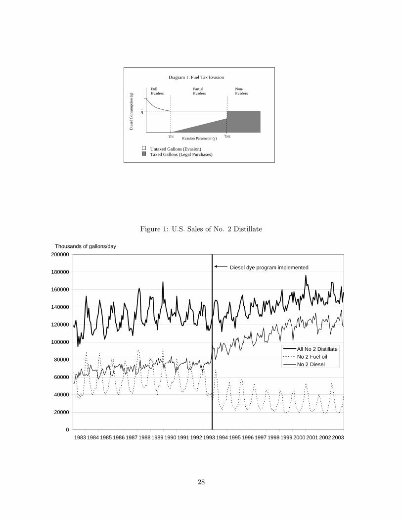
Diagram 1: Fuel Tax Evasion
Evasion Parameter ( )
Untaxed Gallons (Evasion) Taxed Gallons (Legal Purchases)
FE NE
Full Partial Non- Evaders Evaders Evaders
Die
sel C
onsu
mpt
ion
(q)
q
Figure 1: U.S. Sales of No. 2 Distillate
0
20000
40000
60000
80000
100000
120000
140000
160000
180000
200000
1983 1984 1985 1986 1987 1988 1989 1990 1991 1992 1993 1994 1995 1996 1997 1998 1999 2000 2001 2002 2003
All No 2 DistillateNo 2 Fuel oilNo 2 Diesel
Diesel dye program implemented
Thousands of gallons/day
28

Figure 2: Time Series of Diesel Tax Rates (c/gall)
Panel A: Federal Tax Rate
0
5
10
15
20
25
30
1983 1984 1985 1986 1987 1988 1989 1990 1991 1992 1993 1994 1995 1996 1997 1998 1999 2000 2001 2002 2003
Panel B: Average State Tax Rate
0
5
10
15
20
25
1983 1984 1985 1986 1987 1988 1989 1990 1991 1992 1993 1994 1995 1996 1997 1998 1999 2000 2001 2002 2003
Avg. state diesel taxNumber of states changing tax rate
29

Figure 3: Distribution of State Diesel Tax Rates
Panel A: 1983
0
5
10
15
20
25
30
35
0-5 5-10 10-15 15-20 20-25 25-30 30-35
Panel B: 1993
0
5
10
15
20
25
30
35
0-5 5-10 10-15 15-20 20-25 25-30 30-35
Panel C: 2003
0
5
10
15
20
25
30
35
0-5 5-10 10-15 15-20 20-25 25-30 30-35Cents per gallon
30

Figure 4: Average Predicted Versus Actual Log Quantities Sold
Panel A: No. 2 Diesel
5.6
5.8
6
6.2
6.4
6.6
6.8
7
7.2
7.4
7.6
7.8
1983 1984 1985 1986 1987 1988 1989 1990 1991 1992 1993 1994 1995 1996 1997 1998 1999 2000 2001 2002 2003
Panel B: No. 2 Fuel Oil
5
5.5
6
6.5
7
7.5
1983 1984 1985 1986 1987 1988 1989 1990 1991 1992 1993 1994 1995 1996 1997 1998 1999 2000 2001 2002 2003
31
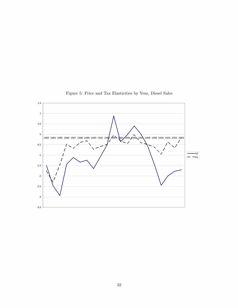
Figure 5: Price and Tax Elasticities by Year, Diesel Sales
-3.5
-3
-2.5
-2
-1.5
-1
-0.5
0
0.5
1
1.5
1983 1984 1985 1986 1987 1988 1989 1990 1991 1992 1993 1994 1995 1996 1997 1998 1999 2000 2001 2002 2003
b2b1
32

Figure 6: Elasticity to 1+Diesel Tax Rate, Fuel Oil Sales
-3
-2
-1
0
1
2
3
4
5
6
1983 1984 1985 1986 1987 1988 1989 1990 1991 1992 1993 1994 1995 1996 1997 1998 1999 2000 2001 2002 2003
33

Table 1: Summary StatisticsPre-Dye Post-Dye
(1) (2)Diesel 1449.31 2315.93
(1855.85) (2134.98)Fuel oil 1262.08 859.15
(1711.04) (1169.89)State + federal diesel tax (c/gall) 30.54 44.47
(7.02) (4.87)Diesel and Fuel Oil Price:
All end users 75.49 81.17(15.32) (18.46)
Residential users 88.68 97.28(14.19) (19.81)
Sold through retail outlets 77.79 82.61(14.21) (17.96)
Other distillates:No. 1 Distillate 67.26 85.22
(94.84) (109.07)No. 4 Distillate 133.26 130.00
(243.26) (219.14)Residual fuel oil 1441.77 1074.25
(2067.73) (1343.51)
Degree days 441.14 433.40(438.22) (419.15)
Missing No. 2 Diesel 0.09 0.20
Missing No. 2 Fuel Oil 0.10 0.24
Fraction of HH using heating oil 0.14Standard errors are in parentheses. Quantity variables are in thousands ofgallons per day. Diesel and fuel oil are chemically equivalent and differ onlyin intended use. Diesel is mostly used for on-road (taxed) purposes, andfuel oil is used for home heating and in industrial boilers. Other distillatesare other fuel formed from the distillation of crude oil. The fraction ofhouseholds using heating oil refers to the reported mode of home heatingin the 1990 Census.
34

Table 2: Log Sales Response to Diesel Dye
Fuel Oil’s ShareLog Diesel Sales Log Fuel Oil Sales of No. 2 Distillate
(1) (2) (3) (4) (5) (6)
Post-dye 0.293 0.256 -0.308 -0.394 -0.113 -0.125(0.033)*** (0.020)*** (0.054)*** (0.032)*** (0.015)*** (0.008)***
Log (p+t) -0.134 0.193 0.063(0.031)*** (0.055)*** (0.009)***
Degree days (X100) -0.026 -0.049 -0.003(0.003)*** (0.008)*** (0.002)*
Deg. days*% HH oil 0.04 0.243 0.038(0.003)*** (0.018)*** (0.003)***
Log of state GSP 0.371 -0.814 -0.149(0.045)*** (0.126)*** (0.014)***
State unemp. rate 0.000 -0.011 -0.000(0.003) (0.008) (0.001)
Quadratic time trend X X X X X XState fixed effects X X XMonth dummies X X XObservations 10606 10236 10236 9866 10061 9710R-squared 0.09 0.96 0.03 0.83 0.12 0.89
Robust standard errors are in parentheses allowing for clustering by state.*,**,*** denote significance at the 90%, 95%, and 99% level, respectively. Post-dye is a variable indicatingthe period after the implementation of the dye program in October of 1993. The variable p+t captures thetax inclusive price of diesel sold through retail outlets. The variable % HH oil represents the percentageof households in the state reporting in the 1990 census using fuel oil for home heating. The price is thatcharged for diesel through retail outlets. The quadratic time trend is allowed to differ in the pre-dye andpost-dye periods.
35

Table 3: Per Capita Sales Response to Diesel Dye
Per Capita Diesel Per Capita Fuel Oil All No. 2 Distillate(1) (2) (3) (4) (5) (6)
Post-dye 0.085 0.067 -0.070 -0.066 0.014 0.005(0.012)*** (0.012)*** (0.012)*** (0.014)*** (0.011) (0.013)
Price + tax -0.001 0.001 0.000(0.000)*** (0.000)*** (0.000)
Degree days (X100) -0.013 -0.021 -0.034(0.003)*** (0.004)*** (0.006)***
Deg. days*% HH oil 0.020 0.123 0.146(0.005)*** (0.014)*** (0.016)***
Log of state GSP 2.384 -11.316 -9.490(6.285) (6.334)* (9.193)
State unemp. rate -0.009 -0.003 -0.010(0.004)** (0.007) (0.007)
Quadratic time trend X X X X X XState fixed effects X X XMonth dummies X X XObservations 10606 10236 10236 9866 11877 11446R-squared 0.86 0.87 0.63 0.77 0.72 0.81
Robust standard errors are in parentheses allowing for clustering by state.*,**,*** denote significance at the 90%, 95%, and 99% level, respectively. The dependent variableis the number of gallons of the stated fuel sold per day in a given state month divided by the statepopulation in that year. For a description of the control variables, please see the notes for Table 2.
36
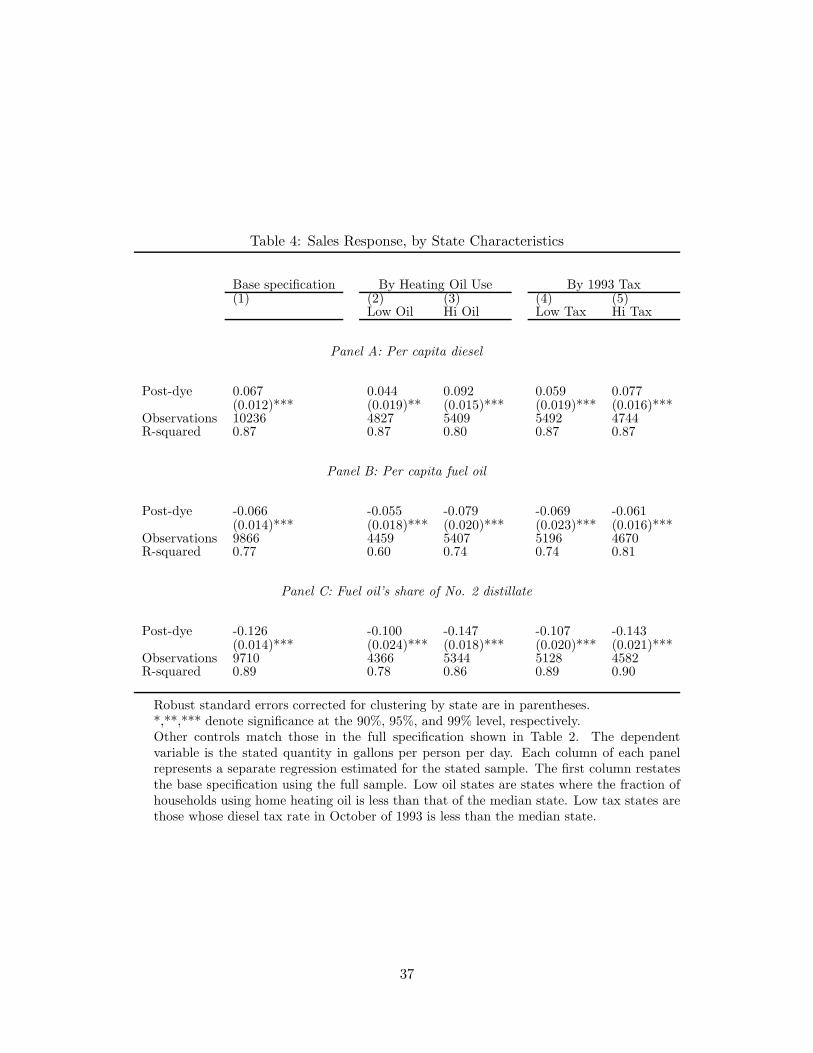
Table 4: Sales Response, by State Characteristics
Base specification By Heating Oil Use By 1993 Tax(1) (2) (3) (4) (5)
Low Oil Hi Oil Low Tax Hi Tax
Panel A: Per capita diesel
Post-dye 0.067 0.044 0.092 0.059 0.077(0.012)*** (0.019)** (0.015)*** (0.019)*** (0.016)***
Observations 10236 4827 5409 5492 4744R-squared 0.87 0.87 0.80 0.87 0.87
Panel B: Per capita fuel oil
Post-dye -0.066 -0.055 -0.079 -0.069 -0.061(0.014)*** (0.018)*** (0.020)*** (0.023)*** (0.016)***
Observations 9866 4459 5407 5196 4670R-squared 0.77 0.60 0.74 0.74 0.81
Panel C: Fuel oil’s share of No. 2 distillate
Post-dye -0.126 -0.100 -0.147 -0.107 -0.143(0.014)*** (0.024)*** (0.018)*** (0.020)*** (0.021)***
Observations 9710 4366 5344 5128 4582R-squared 0.89 0.78 0.86 0.89 0.90
Robust standard errors corrected for clustering by state are in parentheses.*,**,*** denote significance at the 90%, 95%, and 99% level, respectively.Other controls match those in the full specification shown in Table 2. The dependentvariable is the stated quantity in gallons per person per day. Each column of each panelrepresents a separate regression estimated for the stated sample. The first column restatesthe base specification using the full sample. Low oil states are states where the fraction ofhouseholds using home heating oil is less than that of the median state. Low tax states arethose whose diesel tax rate in October of 1993 is less than the median state.
37

Table 5: Fuel Oil Demand Pre- vs. Post-DyeDependent variable: Log Fuel Oil Sales
(1) (2) (3)
Degree days X100 -0.015 -0.046 0.014(0.007)** (0.009)*** (0.006)**
Degree days * HH Oil Fraction 0.211 0.218 0.028(0.032)*** (0.031)*** (0.020)
After * Degree days X100 -0.002 -0.004 0.003(0.006) (0.006) (0.005)
After * Degree days * HH Oil Fraction 0.062 0.063 0.056(0.019)*** (0.018)*** (0.015)***
Month dummies XState-specific month dummies XObservations 10018 10018 10018R-squared 0.30 0.31 0.65
Robust standard errors clustered by state are in parentheses. All specifications include aquadratic pre- and post- time trend and pre- and post- state fixed effects.*,**,*** denote significance at the 90%, 95%, and 99% level, respectively.
Table 6: Price and Tax Elasticity Estimates
Log Diesel Sales Log Fuel Oil Sales
OLS IV OLS IV
Log(1+tax rate) -1.409 -1.333 2.184 2.162(0.506)*** (0.511)** (1.246)* (1.311)+
Post-dye*log(1+tax rate) 0.579 0.597 -1.995 -2.144(0.930) (0.965) (2.246) (2.343)
Log(Price) -0.521 -0.486 0.442 0.862(0.148)*** (0.144)*** (0.407) (0.377)**
Post-dye*log(Price) 0.241 0.258 0.077 -0.657(0.335) (0.359) (0.900) (0.829)
Observations 10236 10236 9866 9866R-squared 0.96 0.96 0.83 0.83
Robust standard errors corrected for clustering by state are in parentheses.*,**,*** denote significance at the 90%, 95%, and 99% level, respectively. +
denotes one-sided significance at the 90% level.Each specification also includes controls identical to those in the full specifi-cation shown in Table 2. The pre-tax price in the diesel specifications is theprice charged through retail outlets.
38