Measuring Global Money Laundering The Walker Gravity … · Measuring Global Money Laundering: “The Walker Gravity Model” JOHN WALKER, BRIGITTE UNGER University of Wollongong,

Measuring Global Money Laundering: “The Walker Gravity Model”

JOHN WALKER, BRIGITTE UNGER

University of Wollongong, Australia; Utrecht University School of Economics *

Measuring global money laundering, the proceeds of transnational crime that are pumped through the financial system worldwide, is still in its infancy. Methods such as case studies, proxy variables, or models for measuring the shadow economy all tend to under- or overestimate money laundering. The model presented here is a gravity model which makes it possible to estimate the flows of illicit funds from and to each jurisdiction in the world and worldwide. This “Walker Model” was first developed in 1994, and used and updated recently. We show that it belongs to the group of gravity models which have recently become popular in international trade theory. Using triangulation, we demonstrate that the original Walker Model estimates are compatible with recent findings on money laundering. Once the scale of money laundering is known, its macroeconomic effects and the impact of crime prevention, regulation and law enforcement effects on money laundering and transnational crime can also be measured.

1. INTRODUCTION

Historically, international efforts to combat transnational crime and money laundering were notoriously “case-oriented,” and it has only been in the last few decades that such notions as “problem-oriented policing,” which involve looking beyond individual cases to the patterns and causal factors, have entered the vocabulary of criminologists and policy makers. Even “crime prevention” is a concept that only became fashionable in developed countries as recently as the 1980s. Neither the preventive nor the problem-oriented concept has yet been widely adopted to address the issues of transnational crime and money laundering, the prevailing responses to which remain firmly in the regulatory and reactive law enforcement models.

* John Walker: Centre for Transnational Crime Prevention, University of Wollongong, NSW

2522, Australia; Brigitte Unger: Utrecht University School of Economics, Janskerkhof 12 3512 BL Utrecht, The Netherlands.

Recently, however, the international community and the literature on law and economics have made quite some efforts and progress to explore and measure the relationship between policy effort and transnational organized crime. The theoretical framework presented by Kugler, Verdier and Zenou (2003) points out that oligopoly-driven market structures in the hands of criminal organizations engage in competition by corrupting public officials in order to avoid punishment and acquire market power over illicit markets. Buscaglia (2008) shows that under such conditions the traditional Becker (1968) and Levitt (1998) hypothesis, that expected higher sanctions and higher probabilities of prosecution work as a deterrence effect for crime, does not hold. An increase in policing and enhanced expected sanctions can produce higher crime rates by making organized crime extend the corruption rings aimed at controlling their territories and feudalizing the state domain in order to gain greater impunity and a reduction in actual expected punishment. There is, hence, a paradox of criminal sanctions where more frequent and stiffer punishments lead to higher levels of organized crime and higher levels of corruption. Buscaglia tests this hypothesis for 107 countries by means of jurimetric analysis.

Data on crime and crime prevention, a prerequisite for this type of study, have improved substantially within the last two decades. In particular, the international community now has quite a detailed knowledge base on the illicit drug economy. The U.N., for example, can zoom in on opium fields on Google Earth and calculate the cultivation and production of opium and cocaine worldwide quite accurately (see UNODC, 2005). The annual U.N. Office on Drugs and Crime International Crop Monitoring Programme Surveys provide annual statistics on the cultivation and production of drugs, as well as prices, yield and the farm gate, and the wholesale and retail market valuations that are calculated from them.1

One important finding of the new literature on criminal organization and transnational crime is that confiscation of assets is an important way to effectively combat crime (Buscaglia, 2008). But what is known about the size of these assets and the flows of income of organized crime? The latest report of the UN states that “one of the most important missing pieces of information concerns the flow of income generated by crime, if, where and how these financial flows intersect with local, national, regional and international economies and their impact on these economies and financial systems.” While relatively much international effort has been put into exploring crime, little effort so far has been made in exploring its financial counterpart.

1 Interestingly, this degree of research effort far exceeds that devoted to the other, non-drug-

related, areas of transnational crime.

822 / REVIEW OF LAW AND ECONOMICS 5:2, 2009

Review of Law & Economics, © 2009 by bepress

The economics of money laundering, which aims to explore the scale and impact of illicit funds, is a relatively new field (see, e.g., Masciandaro et al., 2007;

Unger, 2007). Its efforts and relevance are politically supported by the Financial Action Task Force (FATF), an intergovernmental body created in 1989 by the G-7 to fight money laundering and terrorism financing, which “works to generate the necessary political will to bring about legislative and regulatory reforms in these areas.”2

In 1998, the Managing Director of the International Monetary Fund (IMF), Michel Camdessus, stated in an address to the FATF that “2 to 5 percent of global GDP would probably be a consensus range,” thus about 1.5 trillion US$ of money laundering at that time.3 The method of this estimate could however not be retraced even by academics doing intensive studies within the Fund (see Thoumi, 2003; Truman and Reuter, 2004) and seems more a wet finger approach than serious measuring. What has been less well reported over the years is Camdessus’ assessment of the importance of understanding the extent and nature of money laundering because of its effects on global economies. With a prescience that resonates in the current international financial crisis, he noted that

“This scale poses two sorts of risks: one prudential, the other macroeconomic. Markets and even smaller economies can be corrupted and destabilized. We have seen evidence of this in countries and regions which have harbored large-scale criminal organizations. In the beginning, good and bad monies intermingle, and the country or region appears to prosper, but in the end Gresham’s law operates, and there is a tremendous risk that only the corrupt financiers remain. Lasting damage can clearly be done, when the infrastructure that has been built up to guarantee the integrity of the markets is lost. Even in countries that have not reached this point, the available evidence suggests that the impact of money laundering is large enough that it must be taken into account by macroeconomic policy makers. Money subject to laundering behaves in accordance with particular management principles. There is evidence that it is less productive, and therefore that it contributes minimally, to say the least, to optimization of economic growth. Potential macroeconomic consequences of money laundering include, but are not limited to: inexplicable changes in money demand, greater prudential risks to bank soundness, contamination effects on legal financial transactions, and greater volatility of international capital flows and exchange rates due to unanticipated cross-border asset transfers.” 4

2 http://www.fatf-gafi.org. 3 http://www.imf.org/external/np/speeches/1998/021098.htm. 4 Unger (2007) did a literature survey and identified altogether 25 economic, social, and political

effects of money laundering. Money laundering can also have positive effects, for example, on growth if a country manages to keep the associated crime abroad and only benefits from the additional

The Walker Gravity Model / 823

http://www.bepress.com/rle/vol5/iss2/art2DOI: 10.2202/1555-5879.1418

The “Walker Model” (Walker, 1995, 1999, 2002, 2003a,b) was the first serious attempt at quantifying money laundering worldwide. The 1995 “prototype” model suggested that 2.85 trillion US dollars were laundered globally – exceeding the upper-range figure suggested by Camdessus’ statement, and raising questions on the underestimation of the global extent of fraud.

This model has gained popularity recently. In 2005, Walker used a similar methodology to predict global drug money flows (see UNODC, 2005); in 2006 Unger et al. used the Walker Model to estimate money laundering for the Netherlands, and at the moment the IMF is busy with improving variables and data collection for this model, which remains the leading model for measuring international global money laundering. In the following sections, we will show the historical background of this model and its theoretical foundation, demonstrate and explore its strengths and weaknesses for measuring money laundering, describe its development in the last thirteen years, and identify where to go in the future.

2. HISTORICAL BACKGROUND: MEASURING CRIME

AND MONEY LAUNDERING

2.1. TRANSNATIONAL CRIME DATA

Up until the 1970s statistics were rarely used to analyze patterns in crime. Data collection was still very poor and data were not electronically available. In 1974, when one of us (Walker) was searching for crime data by suburb for a project on behalf of the Melbourne Metropolitan planning agency, the Victoria Police crime analyst pointed to a pile of paper in the corner and invited him to “help himself.” Analyses of international trends in crime were based on police data on recorded crime, a variable that has problems of reliability as well as of international comparability.

“The government are very keen on amassing statistics. They collect them, add them, raise them to the nth power, take the cube root, and prepare wonderful diagrams. But you must never forget that every one of these figures comes, in the first instance, from the village watchman, who just puts down what he damn pleases” - English Economist Sir Josiah Stamp, 1929 5

demand for goods and services created by laundered money. In the long run, however, money laundering will undermine economic, social, and political institutions, and its negative effects will outweigh eventual short-term benefits.

5 http://en.wikipedia.org/wiki/Josiah_Stamp.



Most countries were compiling national crime statistics, but they only measured crime as recorded by police, and were significantly affected by the extent to which victims of crime were willing to report crimes to the police. There were also known problems of accuracy, including suggestions of rigging by police and politicians, as well as the more technical issues of definitions and counting rules. These recorded crime data were compiled by Interpol, and were made available in publicly available reports for those attempting to conduct internationally comparative studies of crime: however, it became clear that there was little consistency between countries and thus attempts to use these data to compare crime levels and trends between countries inevitably failed.

During the 1970s, Crime Victims Surveys were developed in the USA and UK to capture data on a common set of definitions and on unrecorded crime. These were not without their own set of problems, including only being appropriate for a limited range of crime types. They were costly, added to political risks, and initially found little interest in other countries, but they significantly broadened the range of information available on the causes and consequences of crime.

In the 1980s, the U.N. attempted to compile international crime and justice statistics on a common set of definitions. This was done by circulating a standardized questionnaire to justice agencies in member countries.6 This was also problematic, eliciting only a modest response with little consistency between countries in spite of great care being taken to take account of different interpretations and cultures, and initial analyses of the data were discouraging. Other U.N. research projects at the time included analyses of transnational crime, but these were mostly country-specific, offense-specific, or confined to studies of specific mafia, yakuza, or drug gangs, etc. Transparency International was also experimenting with corruption and bribery indexes.

In 1988, the U.N. introduced its convention against illicit traffic in narcotic drugs and psychotropic substances, and the first International Crime Victims Surveys emerged from a European Union initiative, including questions such as “did you report the crime to police?” and “how much did the crime cost you?” (van Dijk et al., 1990). These first surveys focused on personal and household crimes only. They were complemented in the early 1990s by the International Survey of Crime against Business (van Dijk, 2008), a survey piloted by the U.N., which included similar reporting and cost questions. Australia, UK, Netherlands and South Africa were the founding members of this survey. In 1992, the data from these surveys formed the basis of Estimates of the Costs of Crime in Australia (Walker,

1992), which was promoted by the U.N. as a model for other countries to follow.

6 http://www.unodc.org/unodc/en/data-and-analysis/United-Nations-Surveys-on-Crime-Trends-

and-the-Operations-of-Criminal-Justice-Systems.html.



The second half of the 1990s was an exciting time for criminologists, owing to the progress that was being made in developing new sources of data on crime, which enabled international comparisons of levels of crime incidence, which in turn enabled the identification of crime-specific risk factors and an emphasis on “what works?” types of evaluation studies. In 1996-2000, the UN Office on Drugs and Crime continued to refine and extend the International Crime and Justice Surveys, the International Crime Victims Surveys, and the International Business Crime Surveys. The “Global Report on Crime and Justice” (Newman, 1999) attempted to bring together data on the economics of transnational crime, and attempts were made to survey the characteristics of organized crime groups in different countries.

2.2. ESTIMATES OF THE COSTS OF CRIME

The purpose of doing this sort of internationally comparative data collection and analysis is to identify the common drivers of crime, find out how the reporting of crime varies from country to country, and discover how some societies manage to achieve lower than expected real rates of crime. These analyses form the basis of evidence-based crime prevention and control measures. But while traditional criminology focuses on the offender and the crime, politicians almost universally base their decision-making on the perceived relative costs of alternative issues. So if it can be shown that, for example, crime is seen to impose lower costs on society than disease, then governments will prioritize the fight against disease; if drug crime imposes higher perceived costs than, say, fraud and corruption, then governments will prioritize the fight against drugs. The policy importance of “costs of crime” figures cannot be overstated – cost-benefit analyses implicitly or explicitly form the basis of evidence-based government priority settings.

To estimate the costs of crime, we need to firstly know the amount of crime – and not only the amount that is recorded by police. We need to know about unrecorded crime as well as recorded crime. We also need to know what the average costs are for each different type of crime, and whether crimes that are not reported to police are less costly than those that are reported. The collection of these data in the Australian component of the International Crime Victims Survey (Walker et al., 1990) provided the basis for estimates of the costs of crime in Australia. Fraud is easily the most costly type of crime in Australia, because it is widespread and many instances of fraud incur very high costs to the victims.

The total estimated cost of crime for Australia amounted to between 11 and 20 billion AUD$, around 2.5% of GDP. The total cost of the Australian criminal justice system at the time approached 4 to 5 billion, about one-third of the estimated costs of crime (Walker, 1992); subsequent studies seem to suggest



that these ratios are common, at least in countries similar to Australia.7 These figures had quite an impact on Australian politics, and made the effort to combat fraud, which has costs that are ten times higher than drugs, very much more a priority than previously.

2.3. METHODS FOR ESTIMATING MONEY LAUNDERING

In 1989, the Financial Action Task Force’s “Working Group on Statistics and Methods” report “Narcotics Money Laundering – Assessment of the Scale of the Problem” had noted the lack of reliable data to measure money laundering. In 1990, the European Union introduced its Convention on Laundering, Search, Seizure and Confiscation of the Proceeds from Crime, and the FATF’s “Forty Recommendations” on the prevention of money laundering were published.

So, it was in this context that, in 1995, AUSTRAC, the Australian Financial Intelligence Unit, commissioned Estimates of the Extent of Money Laundering in Australia (Walker, 1995) and, in 1996, presented it to the FATF as a potential model for other countries to follow. Criticism focused on the poor quality of the data and the methodology’s reliance on “expert knowledge,” but it was generally agreed that expert knowledge was a reasonable approach so long as it was used only to fill in gaps in statistical evidence.

While other researchers (e.g., Levi and Gold, 1994) were trying to analyze financial data, including data on “suspicious transactions,” to identify the extent of money laundering, the Walker Model approach was quite different. Since money laundering involves many stages – “placement” (e.g., putting illicit cash money at a bank), “layering” (pumping money around the globe to hide its illicit origin) and “integration” (investing cleaned money) – and the same money may go through many different transactions in the laundering process, counting financial transaction data was therefore certain to involve double – or even more – counting. Worse, counting suspicious transactions was certain to include large errors both ways (“suspicious” transactions that are actually legitimate, and “legitimate” transactions that are actually criminal).

By focusing only on “suspicious transactions,” such researchers substantially underestimated the scale of money laundering. Dutch criminologists also thought of money laundering as a minor event. In the Netherlands, criminologists Meloen et al. (2003) analyzed 52 criminal cases wherein property had been confiscated (ontnemingszaken in Dutch) from criminals related to money laundering. These 52 cases totalled €100 million in laundered funds. The problem with this kind of approach is that it is unclear how representative the data are. Do the 52 money launderers who were caught stand for 0.5 percent, 5 percent, 10 percent or

7 See, for example, Canadian estimates discussed in Wigley and Geary (1999).



50 percent of the money launderers in the Netherlands? Are those launderers caught representative of all money launderers, or are only specific offenders (the stupid ones) caught? Empirical studies have their own dynamics. Guided by this study which gives very interesting insights into the behavior of money launderers, Dutch criminologists up until 2007 thought that money laundering in the Netherlands was negligible and they thus heavily underestimated the problem (see, e.g., van Duyne, 2006a).

Police files and the study of them suffer not only from underestimation of the size of the problem, but also suffer from the fact that they are useless for estimating national or global money laundering, because they have an intrinsic logical problem when aggregated. The stricter the fight against launderers, the more eagerly the police will record money laundering cases. When police files are used in order to make general statements about laundering, the data would show that money laundering increases with stricter anti-money laundering policy. Logically one would want money laundering to decline with more and effective policy and not to increase.

Money laundering can also be measured by means of surveys. Experts and law enforcement agents can be interrogated. However, surveys also suffer from diverse biases. The sample might not be representative and the people interviewed or questioned might have had their own perception biases. To give an example, there might be an overestimation of money laundering by those authorities responsible for combating money laundering because fighting laundering is their daily business and center of focus. At the same time, there might also be an underestimation by the same people if they feel that they fulfill their task of fighting crime efficiently and do their job well. However, while perception biases, interpretation biases, biases from non-response and sample biases might affect these data, sometimes they can provide important insights, especially when dealing with otherwise unobservable facts.

Money laundering can also be estimated using proxy variables. Tanzi (1997) from the IMF used the difference between money supply and money circulating in the US economy in order to estimate money laundering. He estimated that US$5 billion per year was being taken out of the US in cash through the illegal drugs trade in 1984 and thus missing from the money supply. Even then, he warned that this creates a potential instability for the world financial system because of the possibility that these dollars could be unloaded in exchange for foreign currency. However, his analysis ignores offense types other than drugs, restricts itself to the money which leaves a country in cash, and does not take into account using the regular financial system or trade to transfer illicit funds.

Another way to measure money laundering is to use approaches from measuring the shadow economy to measuring money laundering, such as the



DYMIMIC (dynamic multiple-indicators multiple-causes) model. It uses two sets of observable variables and links them as a proxy to the unobservable variable. One set of observable variables is the causes (for the shadow economy or for money laundering) such as regulations, taxation and prosecutions. The other set is called indicators. These observable variables parallel money laundering and include the growing demand for money, less official growth and/or increases in crime rates. So, if for example money laundering prosecution increases by x percent, and if parallel to this the crime rate goes down by y percent, the model would conclude that money laundering has declined by z percent. Schneider (2006) uses this approach to estimate the shadow economy for 145 countries. Recently he has also applied it to money laundering (Schneider, 2007). One problem with this approach is that the choice of cause and indicator variables is arbitrary and not reinforced theoretically. The DYMIMIC model uses factor analysis to determine how well the different cause variables explain the unobservable variable and those that can be grouped together. The same is then done for the indicator variables. This means statistics decide which indicators form the relevant bundle of causes of the shadow economy (or money laundering) and which are relevant for the parallel indicators of a shadow economy (or money laundering). Indicators are classified into sub-groups that are supposed to represent parts of the unobservable variable. But, again, statistics cannot replace theory. Nevertheless, the method identifies the variables that are highly correlated and measure the same part of the proxy variable, and reduces redundancies in the choice of proxy variables.

So far, of all of these models, the Walker Model (see further under 3.4.) still seems the most promising. In particular, because it can be used for all countries and jurisdictions in the world and because it can be given a theoretical underpinning which is much stronger and more promising than all of the other global money laundering measuring approaches identified so far. Measuring money laundering needs a combination of criminology, economics and finance, which are all included in the Walker Model.

3. THE WALKER MODEL FOR ESTIMATING MONEY

LAUNDERING

An important inspiration for measuring transnational crime flows comes from the Input-Output (Leontief, 1986) model – long used by economists both as the basis for economic modelling and – in the communist countries – as the basis for state planning. In the version that explains international trade, producer countries send their products and services to consumer countries (whether they are “legal”



products and services or illegal ones). The “Total” column must be equal to total production in each country, and the “Total” row must be equal to the total consumption in each country. The model therefore contains an automatic error-checking mechanism. This is very important when studying the economics of transnational crime, because we know how poor crime statistics can be, and how they are affected by the secrecy surrounding illegal activities.

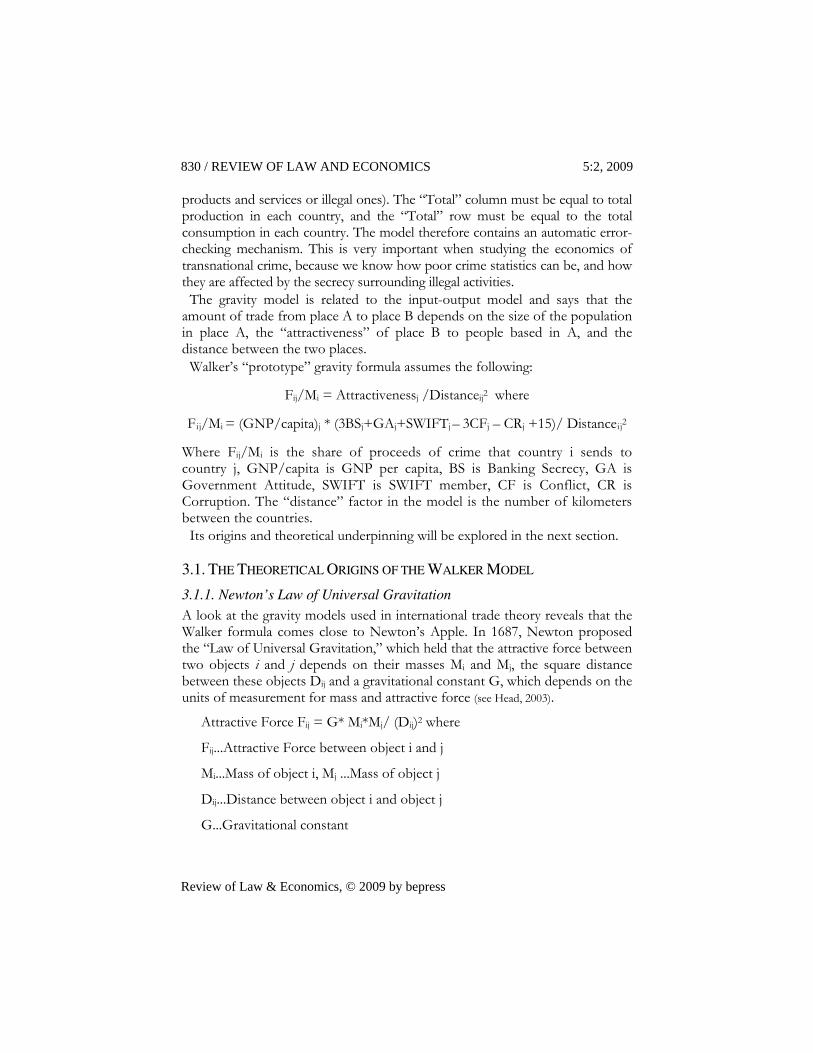
The gravity model is related to the input-output model and says that the amount of trade from place A to place B depends on the size of the population in place A, the “attractiveness” of place B to people based in A, and the distance between the two places.

Walker’s “prototype” gravity formula assumes the following:

Fij/Mi = Attractivenessj /Distanceij2 where

F ij/Mi = (GNP/capita)j * (3BSj+GAj+SWIFTj – 3CFj – CRj +15)/ Distanceij2

Where Fij/Mi is the share of proceeds of crime that country i sends to country j, GNP/capita is GNP per capita, BS is Banking Secrecy, GA is Government Attitude, SWIFT is SWIFT member, CF is Conflict, CR is Corruption. The “distance” factor in the model is the number of kilometers between the countries.

Its origins and theoretical underpinning will be explored in the next section.

3.1. THE THEORETICAL ORIGINS OF THE WALKER MODEL

3.1.1. Newton’s Law of Universal Gravitation

A look at the gravity models used in international trade theory reveals that the Walker formula comes close to Newton’s Apple. In 1687, Newton proposed the “Law of Universal Gravitation,” which held that the attractive force between two objects i and j depends on their masses Mi and Mj, the square distance between these objects Dij and a gravitational constant G, which depends on the units of measurement for mass and attractive force (see Head, 2003).

Attractive Force Fij = G* Mi*Mj/ (Dij)2 where

Fij...Attractive Force between object i and j

Mi...Mass of object i, Mj ...Mass of object j

Dij...Distance between object i and object j

G...Gravitational constant



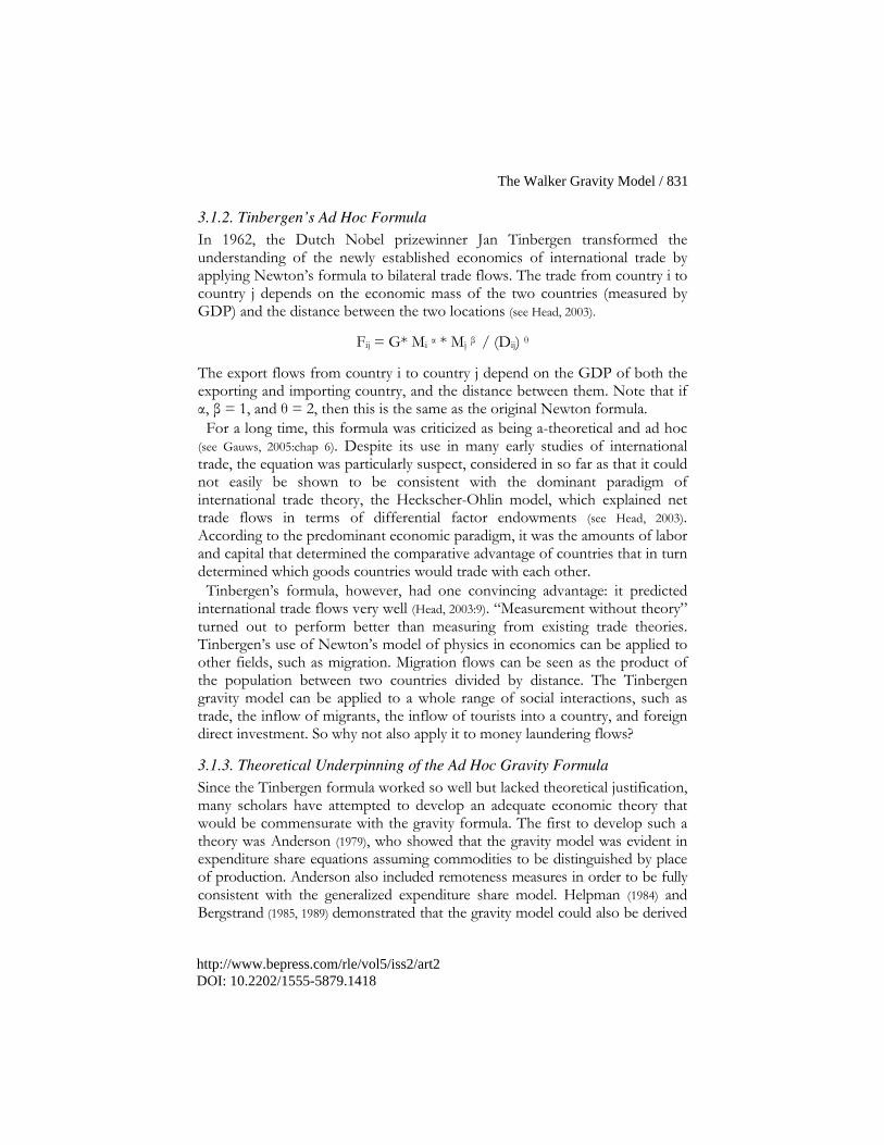
3.1.2. Tinbergen’s Ad Hoc Formula

In 1962, the Dutch Nobel prizewinner Jan Tinbergen transformed the understanding of the newly established economics of international trade by applying Newton’s formula to bilateral trade flows. The trade from country i to country j depends on the economic mass of the two countries (measured by GDP) and the distance between the two locations (see Head, 2003).

Fij = G* Mi α * Mj β / (Dij) θ

The export flows from country i to country j depend on the GDP of both the exporting and importing country, and the distance between them. Note that if α, β = 1, and θ = 2, then this is the same as the original Newton formula.

For a long time, this formula was criticized as being a-theoretical and ad hoc (see Gauws, 2005:chap 6). Despite its use in many early studies of international trade, the equation was particularly suspect, considered in so far as that it could not easily be shown to be consistent with the dominant paradigm of international trade theory, the Heckscher-Ohlin model, which explained net trade flows in terms of differential factor endowments (see Head, 2003). According to the predominant economic paradigm, it was the amounts of labor and capital that determined the comparative advantage of countries that in turn determined which goods countries would trade with each other.

Tinbergen’s formula, however, had one convincing advantage: it predicted international trade flows very well (Head, 2003:9). “Measurement without theory” turned out to perform better than measuring from existing trade theories. Tinbergen’s use of Newton’s model of physics in economics can be applied to other fields, such as migration. Migration flows can be seen as the product of the population between two countries divided by distance. The Tinbergen gravity model can be applied to a whole range of social interactions, such as trade, the inflow of migrants, the inflow of tourists into a country, and foreign direct investment. So why not also apply it to money laundering flows?

3.1.3. Theoretical Underpinning of the Ad Hoc Gravity Formula

Since the Tinbergen formula worked so well but lacked theoretical justification, many scholars have attempted to develop an adequate economic theory that would be commensurate with the gravity formula. The first to develop such a theory was Anderson (1979), who showed that the gravity model was evident in expenditure share equations assuming commodities to be distinguished by place of production. Anderson also included remoteness measures in order to be fully consistent with the generalized expenditure share model. Helpman (1984) and Bergstrand (1985, 1989) demonstrated that the gravity model could also be derived



from models of trade in differentiated products. Deardorff (1998) showed that a suitable modelling of transport costs produces the gravity equation as an estimation, even for the Heckscher-Ohlin model (for an overview, see Helliwell, 2000). The theoretical basis for the Tinbergen formula as applied to trade can be seen in the following (Head, 2003:4).

The trade flows from country i to country j Fij = sij*Mj

where sij is the share of country j’s income spent for goods from country i. This share lies between 0 and 1, increases according to function g, if country i produces a greater variety of goods (ni) or a higher quality of goods (larger mi). This share also should decrease due to trade barriers such as distance. One can write this as:

sij = g(mi, ni, Dij) / Σl g (ml , nl , Dl j)

Depending on the trade theory used, either mi=1 (which means all products from a country have the same average quality) or ni=1 (each country exports

only one single good). l = 1...L are all countries in the world.

Under the assumption that mi=1 and that all firms q are of the same size, the number of products ni = Mi/q. The higher the income of the country, the more products will be produced, and the larger the firm size in the country, the less variety will be produced (this follows from monopolistic trade models a la Dixit-Stiglitz (see Head, 2003:4), which shows that monopolists produce less variety than firms under perfect competition (see Head, 2003:4f). From these assumptions, and after some modification, it follows that

sij = Mi Dij – θ Rj where Rj = 1/ Σl h (Ml , Dl j

– θ)

From this follows Newton-Tinbergen’s formula

Fij = Rj * Mi*Mj / Dij θ

Now, R j has replaced the constant factor G of the old gravity formula. For a long time it was interpreted as a constant across countries. In more recent literature, it is the remoteness factor. Rj stands for each importer’s set of alternatives. Countries that have many nearby sources of goods themselves will have a low value of R j and, therefore, import less. This factor of “remoteness” explains why country groups that have the same distance from each other might still have different trade flows. The remoteness measure also includes Mi/Dii, the distance of the country from itself. Head (2003) suggests taking the square root of the country’s area multiplied by about 0.4 as an approximation for this internal distance. Other authors (Helliwell, 2000) just use a value of 1 instead.



3.1.4. The Role of Distance for Trade Flows

Distance is important for trade flows because it is a proxy for transport costs. It also indicates the time elapsed during shipment, the damage or loss of the good which can occur when time elapses (ship sinks in a storm), or when the good spoils. It also can indicate the loss of the market, for example when the purchaser is unable to pay once the merchandise arrives. Distance also stands for communication costs; it is a proxy for the possibility of personal contact between managers, customers, i.e. for informal contacts which cannot be sent over a wire. Distance can also be seen in a wider perspective as transaction costs, such as the search for trading opportunities or the establishment of trust between partners.

The distance indicator used by Walker (1995) assumes a similar importance for money laundering flows. Though physical distance is less important for money flows, since money cannot perish, and transportation costs are negligible given that money can be sent around the globe at the click of a mouse, the communication costs, transaction costs and cultural barriers might still be important. Therefore, the roles of cultural distance (clashes in negotiation style, language, etc. (Head, 2003:8)), of historical common backgrounds, and of trade relations have to be emphasized more in money laundering gravity models.

3.1.5. The Role of Common Language and Colonial Links

Speaking a common language and sharing a common history and cultural background can lower transaction costs. “Two countries that speak the same language will trade twice to three times as much as pairs that do not share a common language” (Head, 2003; see especially the works of Helliwell, e.g., Helliwell, 2000). This aspect seems captured well in the Walker Model. The only assumption is that what holds for legal trade also holds for illegal transactions.

3.1.6. The Role of Per Capita Income

The gravity model has been augmented by welfare concerns, expressed in the variable “income per capita.” This takes into account that richer countries tend to trade more. The Walker Model assumes the same for money laundering. Richer countries attract more money laundering funds from poorer countries. However, gravity models usually also include a variable for mass (i.e., income), and not only for welfare (income per capita). The original Walker Model did not include a mass variable, since the money laundering of small islands would be overwhelmed by a giant like the US if one included volume variables. But it will certainly need some serious thought on how to justify this dropping of one of the apples’ masses in the formula.8

8 We owe this point to Jaap Bikker.



3.1.7. The Role of Borders

McCallum (1995) claimed that borders still matter as far as trade is concerned. He compares trade between two Canadian provinces to trade between Canadian provinces and US states and shows that borders are a barrier to trade.

Countries trade more if they have no border than if they have one. But when borders exist, it is better for trade to share a border than to be further apart. Trade is about 65% higher if countries share the same border than if they do not have a common border (Head, 2003). So the Netherlands, for example, will trade more with Belgium than with France, even if one corrected for the difference in distance, just because they share a border. This means that if one takes coordinates of capitals and their distance to each other (as we did), one might overestimate the effective distance, because neighboring countries often engage in large volume border trade.9

3.2. MODELLING MONEY LAUNDERING: LESSONS LEARNED FROM

INTERNATIONAL TRADE THEORY

The formula that was suggested in Walker (1995) is very similar to the gravity model. It shares the beginner’s fate regarding this kind of model: namely, to be called ad hoc and a-theoretical. International trade theory, from the Heckscher Ohlin to the Dixit-Stiglitz and Krugman models, shares important theoretical synergies with the Walker Model. One can also hope that the theoretical underpinning of the Walker Model will not take as long as the microeconomic theoretical underpinning of the gravity formula by international trade theory. While the Tinbergen formula could always take the credit for predicting trade flows so accurately, the Walker Model has thus far not received the same degree of acknowledgement. This is for the simple reason that the flows of money laundering stay in the dark and are unobservable. This means that it is not possible to assess the quality of the formula, and the effectiveness of the fit and of forecasting. However, there are many parallels between flows of laundered money and FDI, and the gravity model has been shown to be valid and theoretically sound in these contexts.

As already mentioned, Walker’s “prototype” gravity formula assumes:

F ij/Mi = (GNP/capita)j * (3BSj+GAj+SWIFTj – 3CFj – CRj +15)/ Distanceij2

where GNP/capita is GNP per capita, BS is Banking Secrecy, GA is Government Attitude, SWIFT is SWIFT member, CF is Conflict, CR is Corruption.

9 We owe this point to Thijs Knaap.



If one compares this to the original gravity model, the Walker Model assumes, Rj=(3BSj+GAj+SWIFTj-3CFj-CRj+15) and Mj=(GNP/capita)j. The flow formula is divided by Mi. Mi represents the proceeds of crime in the sending country. In the receiving country the ‘mass’ is welfare (GNP per capita). All the variables relevant for money laundering have been captured in the remoteness variable. The gravitational “masses” of the two objects country i and country j have been assumed to be GNP per capita and money generated for laundering, respectively.

For the distance indicator Dij, the original Walker Model assumed Θ = 2 and used the squared kilometre distance between capitals. As mentioned above, this can overestimate the effective distance due to intense cross-border trade. Unger et al. (2006) opted for Θ = 1, using linear and not squared distance. This is backed up by the fact that many trade gravity equations come up with this coefficient as well (Helliwell, 2000).10

As a next step, the assumptions of money laundering have to be studied more carefully. What do traders and FDI actors have in common with money launderers, and what not? There is still some modeling necessary in order to move from the gravity model to a money laundering model, but given the progress that international trade theory has made, there is optimism that this can happen soon. The money laundering debate can draw on a long history of developments and findings in economic trade theory.

What is still not captured in this and the Walker Model is the full layering phase of money laundering (money laundering is measured at the first phase, at placement, when it is generated and invested domestically or sent abroad). But while the second phase of money laundering, when money is transferred all over the globe in order to hide its origin, is much higher in volume and much more prone to all kinds of financial tricks and sophisticated constructions, it is only sporadically treated. The advantage of avoiding double counting is set against the disadvantage of underestimating actual gross criminal flows.

3.3. ASSUMPTIONS OF THE WALKER MODEL

� Crime generates income in all countries.

� Income from crime depends on the prevalence of different types of crime and the average proceeds per crime.

10 We owe this point to Thijs Knaap. Economists usually claim to be very precise. They have

applied Newton’s principles to economics when creating a theory of exchange. It is therefore not without irony that physics rightly complains that economists turn the universe around when modifying Newton’s formula. The universe would collapse if Newton’s distance square term were changed by even a marginal amount, let us say from 2 to 1.999. When done so in trade equations, the economic system apparently appears to be quite robust.



� Sophisticated and organized crimes generate more income per crime than simpler and individual crimes.

� In general, richer countries generate more income per crime than poor ones.

� Income inequality or corruption may support a rich criminal class even in a poor country.

� Not all criminal income is laundered – even criminals have to eat, sleep, drive fast cars, and pay accountants and lawyers.

These are all supportable assumptions, in the absence of any existing research of this kind. The model has been populated using crime data from the U.N.’s most recent survey results for each country, using regional average rates per population, multiplied by UNDP population data, for countries where no crime data were available. Walker took the relative “proceeds per recorded crime” for each type of crime from his own Australian analysis, adjusted by UNDP data on GDP per capita.

The assumptions built into the model about laundering processes were:

� Not all laundered money leaves the country – some countries' finance sectors provide perfect cover for local launderers.

� Countries where official corruption is common provide benign environments for launderers.

� Laundered money seeks countries with attractive banking regimes, including

– Tax havens,

– "No questions asked" banking,

– Countries with stable economies and low risk.

� Trading, ethnic and linguistic links will determine launderers' preferred destinations – i.e., other things being equal, "hot" money will be attracted to those havens with trading, ethnic, linguistic or geographic links to the generating country.

4. ESTIMATES OF MONEY LAUNDERING FROM THE

WALKER MODEL

To measure money laundering, one must start from “how much crime is there?” and “how much profit is there in the crime?,” and then ask “what proportions of the profits are laundered.” Only then can one address the questions of “where does it go for laundering?” and “what impact does it have on society?”

Thinking further along these lines, it becomes clear that the costs of crime are part of the economy. Proceeds of crime are a subset of the costs. Some proceeds of crime are laundered, but some money is simply spent by the criminals and does not go through any laundering-like process. Some laundered money also comes



from outside the economy, from crimes committed in other countries. The “known” components are very small subsets of their respective estimated totals.

Since September 2001, the FATF has also included terrorism financing in the money laundering definition. Indeed, terrorists can use laundered money to commit their crimes, but terrorist finance is different from the proceeds of crime – it may not have criminal origins, is not necessarily laundered, and the available data suggest that terrorists do not need to launder large amounts of money.

This means that, not only might we be able to find upper and lower limits to our estimates of the proceeds of crime, based on the likely extent and profitability of crime, but we can also use a wide range of other economic data, including estimates of the size of the economy and of imports and exports, to triangulate towards the most credible estimates of the extent of economic crime and money laundering.

Figure 1. An Economic Model of Crime, Money Laundering

and Terrorist Financing

Walker (1995) estimated the proceeds of crime in Australia, and the proportion of those proceeds that are likely to be laundered. The paper starts from the estimates of the extent of recorded and unrecorded crime, and takes only the property loss components of the costs as being equal to the proceeds of crime. These proceeds sometimes have to be heavily discounted, depending on the crime type, because of course if you are selling stolen goods, you will happily accept a lower than market value price for them. However, when the crime is fraud, there are no actual goods to dispose of, so the income from fraud is



almost all proceeds of crime. Finding no actual data that could measure the extent of laundering, Walker (1995) conducted an expert survey to determine the proportions of proceeds likely to be laundered. The proportions differed between crime types, and in general the smaller the returns per crime, the less likely that the proceeds would be laundered.

Table 1. The Original Walker Model

Estimated Proceeds of Crime and Money Laundering in Australia, 1994

Crime Category Estimated Implied ML Estimates for Australia ($mill) Proceeds of Crime Min Mid Max

Homicide Max $2.75m <1 <1 <1 Robbery & Extortion $74.4m <1 22 45 Other Violence Min $3.31m <1 <1 <1 Breaking and Entering $714.4m 14 71 500 Insurance Fraud $1530m 38 77 - 153 306 Business Fraud $375 - $900m 56 225 - 540 900 Other Fraud $750m 38 113 - 188 600 Motor Vehicle Thefts $533.6m 27 53 - 187 480 Other Thefts $462 -1636m 8 82 - 116 347 Environmental Crime $5.25 -16.45m <1 <1 - 2 8 Illicit Drugs $1500m 300 750 - 1050 1350

Total $5951 - $7661m 402 1394 - 2328 4536

Source: Walker (1995)

Figure 2. Estimates of Money Laundering in and through Australia in 1996



In a total Australian economy of (then) $380 billion, it was estimated that the costs of crime were $11-21 billion per annum, of which $6-8 billion were proceeds of crime. Of these, between $0.4-4.5 billion was laundered.

The most likely figure for money laundering was AUD$3.5 billion per annum, generated by crime in Australia and laundered either in Australia or elsewhere, with the bulk being generated by fraud and then drugs.

An update of this work was conducted in 2005, again involving surveys of Australian law enforcement officials and researchers both in Australia and overseas, along with analysis of some official statistics, including data held by AUSTRAC, the Australian Financial Intelligence Unit, but this time also including requests for information from foreign financial intelligence units (FIUs). A literature review was conducted to identify any methodological breakthroughs that might have occurred in the intervening decade – with little to indicate any major progress. The process again provided a range of estimates, suggesting that crime in Australia in 2004 generated between AUD$2.8 billion and AUD$6.3 billion, with the most likely figure being in the vicinity of AUD$4.5 billion.

The lower of these estimates was based on the results of an expert survey and considerable local knowledge of Australia and the major crimes that come to official notice (see Table 2). It is likely, if anything, to err on the low side, because the survey responses may have underestimated the extent or the profits of crimes that never come to public notice, including both fraud and drug crimes.

Table 2. Estimated Proceeds of Crime and Money Laundering in Australia, 2004 based on Expert Survey Information (lower estimate)

Crime Category Estimated Estimated Estimate of Proceeds of Crime % Laundered Money Laundered (AUD millions)

Drug Crime 382 83.0 317 Excise, Tax Evasion 1000 66.7 667 Fraud 887 64.5 572 Arms Trading/Trafficking 31 67.5 21 Illegal Gambling 9 75.0 7 Theft 90 62.5 56 Extortion 12 73.3 9 Stock/Equity Market Fraud 90 90.0 81 Homicide 13 93.3 12 Arson/ Property Damage 63 66.7 42 Illegal Prostitution 31 74.2 23 Environmental Crime 4 83.3 3 Illegal Immigration/People Trafficking 31 73.3 22 Computer Crime 186 67.1 125 ID Fraud 1000 85.0 850

Total 3827.2 2806 Source: Walker (2005)



The higher estimate was derived from an analysis of the costs of property crime in Australia, and the potential profits of the illicit drug trade (see Table 3). It specifically addresses the issue of unrecorded crime, and is thus less susceptible to that type of error, but it may be overestimating the likelihood that those unrecorded frauds, and the illicit drug retail market in Australia, actually generate launderable amounts of proceeds. These estimates relate to proceeds of crime generated in Australia and laundered either within Australia (internal ML) or outside Australia (outgoing ML).

Table 3. Estimated Proceeds of Crime and Money Laundering in Australia, 2004

based on Costs of Crime Estimates (higher estimate)

Crime Category Recorded Estimated Property Total Est. Est. % Implied Crime Incidence Stolen & Property % Proceeds Laundered Money 2001 a 2001 a Damaged a Losses a Proceeds b Lnder’d

(000s) (000s) (AUD/ Incident) (AUD mill.) (AUD mill.) (AUD mill.)

Robbery 27 168 800 134 80.0 107 30.0 b 32 Residential Burglary 275 819 1,100 901 80.0 721 10.0 b 72 Non-Res. Burglary 160 176 2,400 422 80.0 338 10.0 b 34 Theft of Motor Veh. 140 147 4,000 588 80.0 470 35.0 b 165 Shoplifting 73 7,304 100 730 80.0 584 5.0 b 29 Theft from Motor Veh. 266 956 270 258 80.0 206 5.0 b 10 Other Theft 390 1,769 200 354 80.0 283 5.0 b 14 Criminal Damage 319 1,914 350 670 1.0 7 0 b 0 Arson 1,350 1.0 14 0 b 0 Fraud 5,880 75-90.0 4,851 69.4 c 3,367

Drugs 3,500 d 83.3 c 2,915

Total 11,287 11,081 6,282

Notes: a = Mayhew, 2003; b = Walker, 1995 Survey; c = Walker, 2005 Survey; d = based on UNODC, 2005.

Source: Walker (2005)

This range AUD$2.8-6.3 billion is clearly well below the range derived from the Camdessus / IMF estimate based on the proportion of GDP. However, in recent years, researchers (Zdanowicz, 2003) have identified significant areas of hard-to-quantify shadow economy and transfer pricing practices, not generally treated as criminal offenses, but probably involving significant underpayment of tax. If transfer pricing (that is, the manipulation of import and export prices to launder funds between countries) affects Australia to the same extent as that reported for the US, it could significantly increase the estimated money laundered through Australia. Owing to a lack of research in other countries, it is not otherwise possible to estimate the extent of foreign proceeds of crime being laundered through Australia.



5. REVISIONS OF THE WALKER MODEL

5.1. A REVISED WALKER MODEL FOR THE NETHERLANDS

The Walker Model consists of two parts. First it calculates the proceeds from domestic crime that are being laundered, and second it estimates the proceeds from foreign crime that flow into a country for laundering. It is the second part that is the more controversial one in the debate on money laundering.

Money can be laundered in the country in which it was generated or sent to another country or countries for laundering. An important point within this model is that as soon as money has travelled (flowed) at least once, it is “white-washed,” or laundered. This model only counts this first transaction involving the placement of funds. Although “hot money” can be moved on multiple occasions in efforts to disguise its criminal origins, this model does not count each of these transactions, or movement of funds, in order to avoid double counting.

The following formula shows the revised Walker formula as estimated by Unger et al. (2006) for the Netherlands. With this Unger and colleagues followed Walker’s 1995 advice to improve some of the variables.

Percentage of World Criminal Money Flowing Into a Country X (The Netherlands)

Attractiveness = f (GDP per capita, Bank Secrecy, Anti-Money Laundering Policy, SWIFT Membership, Financial Deposits, Conflict, Corruption, Egmont Group)

11

Distance deterrence = f (Language, Colonial Background, Physical Distance)

The formula shows the percentage P of country yi’s (e.g., the US) criminal money flowing to a country X (the Netherlands). This percentage of the US total money for laundering sent to the Netherlands depends on how attractive the Netherlands are for the US (attractiveness yi) and on the distance between the Netherlands and the US (dist (X, yi)). The first part of the right-hand side of the equation simply guarantees that all shares sent by each country add up to 100%.

The Netherlands will be more attractive for launderers based in foreign countries such as the US if it has a higher GDP per capita (because money hides more easily in rich economies than in poor ones), if it has high bank secrecy, if it has the technological means to transfer money quickly (such as being a SWIFT

11 Modifications to the original “Walker Model” are in bold.



member), and if it has low conflict and corruption so that criminals do not have to fear losing their laundered money. We added to this both another variable for strict anti-money laundering policy, namely being a member of the Egmont Group (a group which was established and meets in the Dutch village Egmont aan de Zee in order to combat money laundering), and the variable Financial Deposits. This last variable is meant to express the fact that large financial centers will be more attractive for launderers because they have the expertise and financial skills to handle large amounts of money discreetly.

For the distance deterrence index, Walker’s 1995 suggestions were followed by including social and cultural distance variables, as well as geographical distance. If two countries speak the same language, if they share a common colonial background, and if they are top trading partners for each other, they have more common links and hence less “distance” to each other, than if they do not have these joint experiences. The closer countries are to each other, the lower the distance between them, the more laundering will take place. A precise description of how we measured the variables can be found in Unger et al. (2006).

According to Unger et al. (2006), about 14.5 billion Euro of dirty money was sent to the Netherlands in 2005. The main sending countries were the US, Russia, Italy, Germany, the UK and France. In the Netherlands another 4 billion Euro was laundered from proceeds of Dutch crime (drugs and fraud mainly). This means that the Netherlands has to face about 18.5 billion Euro money laundering yearly, which amounts to about 5 percent of the Dutch GDP. The Netherlands seems to be mainly a through-flow country for laundering. From suspicious transaction reports of the Dutch FIU (MOT, 2005), one can assume that money goes mainly to the Dutch Antilles, Colombia, Turkey and Spain and to Suriname. But the Walker Model would also allow one to precisely calculate how much money flows to which countries. For this, the Walker Model would need to be calculated for all countries and for all (cultural, social and geographic) distances between all countries of the world; something, that was not done in the study.

5.2. INPUT-OUTPUT MODELLING OF THE GLOBAL ILLICIT DRUG TRADE

In late 2004, one of us (Walker) was given an opportunity to estimate the proceeds of the global illicit drug trade, by the United Nations Office on Drugs and Crime. With this, a major point of criticism of the Walker Model – namely its poor crime database – could be removed. As the resulting World Drug Report 2005 states, “A global input-output model was developed building on existing UNODC data collection systems, thus making it replicable as well as allowing for expert opinion to be taken into account” (UNODC, 2005). The model used data published in the 2002-03 World Drug Report, supplemented – where data was missing – with data obtained from Member States over the previous year.



Identical models were used for the analysis of each of the main drug markets: opiates, cocaine, cannabis herb, cannabis resin, amphetamines and ecstasy. The main assumption of this model is that what is being produced, less seizures and less losses, is available for consumption and is consumed. The amounts available for consumption in each sub-region are multiplied with the average parity-adjusted prices of the respective sub-regions to arrive at sub-regional market values. These values are then added up to arrive at the total market value. The model looks at the market sub-regionally. Data inconsistencies are detected in large part because the model looks at the market both from the supply side and from the demand side.

A very simplified region-to-region “distance” matrix was used as the basis for the gravity model component. Pairs of regions were assessed as being “Preferred Supplier,” “Contiguous,” “Distant,” “Remote” or (where for some political or other reason, it was known that trade did not take place between the two regions) “No Trade” pairs. The gravity component was then calibrated to known drug flows. The applicability of input-output modelling to this group of crime types was firmly established by the general acceptance on the part of the research community of the results obtained.

The development of similar models for other important crime types – particularly fraud – is hindered only by the lack of a data collection effort equivalent to that of the UNODC’s Annual Reports Questionnaires, upon which the World Drug Report is based. But with the Input-Output model shown above, the method for doing so is already there.

At the moment one of us (Walker) is working with the IMF to improve the attractiveness indicators of the model, and we are also collecting new data and conducting calibration studies to determine the weights for the variables of the attractiveness indicators.



6. THE ROBUSTNESS OF THE WALKER MODEL

6.1. TRIANGULATION WITH SCHNEIDER’S SHADOW ECONOMY ESTIMATES

One way of testing the quality of estimates of unobservable variables like money laundering is to use triangulation. By comparing the estimates to other estimates, one tries to see how far apart they lie. In particular, where the unobservable variable is logically a subset of another variable that has been quantified (or vice-versa), then the observable variable provides an upper (or lower) limit for the unobservable one. Thus, obviously, total money laundering must be at least as large as “known” money laundering, based on the amounts for which criminal convictions have been obtained. But there are many other – more interesting – triangulations that can be made.

In 2006, Austrian economist Friedrich Schneider published some interesting shadow economy estimates for 145 different countries (Schneider, 2006). A shadow economy is defined as the economic activity in a country that is hidden from authorities – particularly from the tax agency. In many countries, the shadow economy consists mostly of legal activities that are kept hidden for tax avoidance purposes, but logically, since criminals do not report their illegal income to the tax authorities, the proceeds of crime should be a subset of the shadow economy. Some interesting results can be derived by comparing his estimates of shadow economy as a proportion of GDP against GDP per capita.

Unsurprisingly, this analysis suggests that poorer countries have higher percentages of shadow economy than rich countries, and there appears to be a nice J-curve on the graph (Figure 3). Those countries to the lower left of the curve (those with a lower than expected shadow economy – blue, including China) tend to have “command” economies in which the shadow economy is suppressed. In theory, economic crime should be a subset of the shadow economy, and those countries to the right of the line (red) appear to have significant transnational crime, illicit drug production and corrupt business practices.



Figure 3. The Concept of “Excess Shadow Economy”

as a Potential Measure of the Proceeds of Crime

GDP per capita vs. Shadow Economy

42.142.141.6

38.9

35.432.2

2116.8

UAE

Italy

Ireland

NZ

JapanUK

Austria

Switzerland

USA

BoliviaGeorgia

PanamaPeru

Colombia

Morocco

Pakistan

Thailand

Mexico

Vietnam

Uruguay

Belarus

Estonia

Russia

Lao PDRYemen

Iran

China

Mongolia

Australia

0

5,000

10,000

15,000

20,000

25,000

30,000

35,000

40,000

0 20 40 60 80

Shadow Economy as % of GDP

GD

P/c

ap

ita

($

US

) 2

00

1

This analysis seems to identify “excess” shadow economy in some countries, often those with a reputation for “mafia-type” organized crime, including Italy, Russia and Colombia, and the excess can be measured as a proportion of each country’s GDP. It is too soon to know whether this form of analysis can successfully identify the proceeds of organized crime in specific countries – but it is at least extremely interesting. On this basis, the shadow economy in Australia would amount to around AUD$20 billion per year, which is not inconsistent with



the earlier AUD$6-8 billion from crime alone. For the Netherlands the shadow economy estimated by Schneider is 10% of GDP, compared to 5% of GDP estimated for money laundering, which also seems consistent (see Unger, 2007).

6.2. TRIANGULATION WITH U.N. STATISTICS ON SERVICE EXPORTS

A further source of triangulation for estimates of money laundering is the UN’s statistics on services exports.12 When computed as a percentage of GDP, these figures clearly show which countries have unusually strong financial services exports or other services, such as tourism, that could be used for money laundering. These countries include most of the Caribbean tax havens and some of the larger centers including Luxembourg, Switzerland and Singapore. These data can be interpreted as measuring the capacity of the financial sector to support money laundering, which should be an integral part of their “attractiveness” to money launderers.

Figure 4. The Concept of “Capacity to Provide Money Laundering Services”

12 For those countries where disaggregated statistics were available, they showed a strong

positive relationship between financial services exports and total services exports.



6.3. TRIANGULATION WITH A LAW-BASED INDEX FOLLOWING SAVONA

Another aspect of attractiveness to money launderers is the “willingness” of a country’s financial sector to support money laundering. One of us (Walker) was an adviser to the Italian research group TransCrime, led by Professor Ernesto Savona, in their work for the European Union, analyzing the impact of criminal law, administrative regulations, banking law, company law and international co-operation Provisions on money laundering (Savona et al., 2000). Using a simple questionnaire-type framework, the analysis gives a sort of credit rating to each country’s finance sector, depending on how laundry-friendly or laundry-proof it is. As the chart shows, the results of such analysis can identify those countries whose regulations leave gaps for money launderers to wriggle through.

An index can be generated from the responses to the following set of questions:

CRIMINAL LAW 1. Is money laundering punished in your criminal system? 2. Does your legislation provide for a list of crimes as predicate offenses? 3. Do predicate offenses cover all serious crimes? 4. Do predicate offenses cover all crimes? 5. Are there provisions allowing confiscation of assets for an ML offense? 6. Are there special investigative bodies or investigations in relation to ML offenses?

ADMINISTRATIVE REGULATIONS 1. Is there an anti-ML law in the jurisdiction? 2. Are banks covered by the anti-ML law? 3. Are other financial institutions covered by the anti-ML law? 4. Are non-financial institutions covered by the anti-ML law? 5. Are other professions carrying out financial activities covered by the anti-ML law? 6. Are there identity requirements for the institutions covered by the anti-ML law? 7. Do you have suspicious transactions reporting? 8. Is there a central authority (for instance, an FIU) for the collection of suspicious

transactions reports? 9. Is there regular co-operation between banks or other financial institutions and police

authorities?

BANKING LAW 1. Is it prohibited to open a bank account without ID of the beneficial owner? 2. Are there limits to bank secrecy in cases of criminal investigation and prosecution?

COMPANY LAW 1. Is there a minimum share capital required for limited liability companies? 2. Is there a prohibition on bearer shares in limited liability companies? 3. Is there a prohibition on legal entities as directors of limited liability companies? 4. Must a registered office exist for limited liability companies? 5. Is there any form of annual auditing (at least internal) for limited liability companies? 6. Is there a shareholder register for limited liability companies?



INTERNATIONAL CO-OPERATION PROVISIONS 1. Does extradition (at least of foreigners) exist for ML offenses? 2. Is assistance to foreign law enforcement agencies provided in ML investigations? 3. Can law enforcement respond to a request from a foreign country for financial records? 4. Is there provision allowing the sharing of confiscated assets for ML offenses? 5. Has the 1988 UN Convention been ratified?

The index based on these questions correlates strongly with the scores based on the original Walker Model attractiveness index. The potential for money laundering through a country’s banking sector is the product of its capacity to launder and its willingness to launder. These charts suggest that it may be possible to measure both of these aspects to generate a more empirically-based attractiveness index.

Figure 5. Comparing the “Original” Attractiveness Index

with the “Law-Based” Index

6.4. TRIANGULATION WITH BAKER´S FINDINGS

Most critiques of the model attack either the data quality, for which there is no defense other than to ask for some genuine international effort to generate better data, or attack the conclusion that fraud is more important than illicit drugs. The FATF’s easy agreement in 1998 to the proposition that research should focus on



illicit drugs appeared particularly at odds with Walker’s work. Those who focus on drugs and consider them the more important source of laundered money may be simply closing their eyes to all of the fraud that goes on around them.

This view is supported by Raymond Baker’s (2005) interesting work on cross-border flow analysis. It is based only on a review of studies of transnational crime, and the data may not be internally consistent, but this is another essential research technique in its own right. Each of these figures can potentially serve as a credibility check on any estimates we are able to generate.

Table 4. Summary of Estimates of Global Flows of Illicit Finance

Global Flows Low ($US bn) High ($US bn)

Drugs $120 $200 Counterfeit goods $80 $120 Counterfeit currency $3 $3 Human trafficking $12 $15 Illegal arms trade $6 $10 Smuggling $60 $100 Racketeering $50 $100 Crime Subtotal $331 $549 Mispricing $200 $250 Abusive transfer pricing $300 $500 Fake transactions $200 $250 Commercial Subtotal $700 $1000 Corruption $30 $50

Grand Total $1061 $1599

(Source: Baker, 2005)

Baker estimates that criminals in the rich countries around the world are transferring from the poorer countries something like ten times the amount of aid given by the rich countries to the poor. Baker’s estimate for illicit flows from developing countries, $800 billion, closely matches the corresponding results obtained from the Walker Model, $850 billion. The most important reason why we need to focus on the economics of crime and money laundering is that international crime prevention strategies should not only benefit the rich countries.

7. FUTURE CHALLENGES

The Walker Model still seems to be the most reliable and robust method to estimate global money laundering, and thereby the important effects of transnational crime on economic, social and political institutions.

The attractiveness and distance indicator in the Walker Model are a valid first approximation, but are still quite ad hoc. A better micro-foundation for the



Walker Model will be needed in the future. For this, the behavior of money launderers, and in particular what makes them send their money to a specific country, is important. In the Walker Model, each country sends criminal money to all other countries. Some countries receive a smaller share of a country’s criminal money (if they are less attractive and more geographically or socially distant), while others receive a larger share. However, it is very likely that laundered money follows a particular route. To give an example: if Italian launderers always send their drug money only to Turkey, and if Dutch launderers send their ecstasy pill proceeds only to the UK, then the Walker Model, which assumes a large spread of flows of money, would have to be corrected for this.

It seems therefore crucial to continue to cooperate with criminologists to study criminal behavior. The variables in the attractiveness indicator are, though plausible, still arbitrary. In particular, the weights of the variables in the attractiveness and distance indicator are still arbitrary. Maybe large financial centers attract far more laundered money, or small islands without financial centers are far more attractive for launderers than indicated by the global criminal flow model used by the Walker Model.

An economics of crime micro-foundation for the Walker Model would mean that, similarly to international trade theory, behavioral assumptions about money launderers have to be made. The gravity model must be the (reduced form) outcome of their rational calculus of sending their money to another country and possibly getting caught, but potentially making large profits. It was a long way from Tinbergen’s ad hoc formula to the micro foundation for it found in modern trade theory. A similar approach is needed for criminal flows. There is hope that it will take less time to do so.



References

Anderson, J.E. 1979. “A Theoretical Foundation for the Gravity Equation,” 69 American Economic Review 106-16.

Anderson, D. 1999. “The Aggregate Burden of Crime,” 42(2) Journal of Law and Economics 611-42.

Baker, R. 2005. Capitalism's Achilles Heel - Dirty Money and How to Renew the Free-Market System. Hoboken, NJ: John Wiley & Sons.

Becker, Gary. 1968. “Crime and Punishment: An Economic Approach,” 76 Journal of Political Economy 167-217.

Bergstrand, J.H. 1985. “The Gravity Equation in International Trade: Some Microeconomic Foundations and Empirical Evidence,” 67 Review of Economics and Statistics 474-81.

_______. 1989. “The Generalized Gravity Equation, Monopolistic Competition and the Factor-Proportions Theory in International Trade,” 71 Review of Economics and Statistics 143-53.

Buscaglia, Edgardo. 2008. “The Paradox of Expected Punishment: Legal and Economic Factors Determining Success and Failure in the Fight against Organized Crime,” 4(1) Review of Law and Economics 290-317.

Deardorff, A. 1998. “Determinants of Bilateral Trade: Does Gravity Work in a Frictionless World?” in J. Frankel, ed. The Regionalization of the World Economy. Chicago: University of Chicago Press, 7-28.

Dijk, J. van. 2008. The World of Crime – Breaking the Silence on Problems of Security, Justice, and Development Across the World. Thousand Oaks, CA: Sage Publications.

_______, P. Mayhew, and M. Killias. 1990. Experiences of Crime across the World – Key Findings of the 1989 International Crime Survey. Deventer: Kluwer.

Duyne, P.C. van. 2006a. “De stelling van Petrus van Duyne: maak criminelen niet groter dan ze zijn (Do not make launderers appear bigger than they are),” NRC Handelsblad, February 11, 2006 (interview by R. Janssen).

_______. 2006b. “Witwasonderzoek, luchtspiegelingen en de menselijke maat (Money laundering research, fata morgana and the human measure),” Justitiële verkenningen, jrg. 32, nr. 2 2006.

Financial Action Task Force (FATF). 2005. Annual Report. Paris: Organisation for Economic Co-Operation and Development.

Gauws, A.R. 2005. “The Determinants of South African Exports: Critical Policy Implications,” Ph.D University of Pretoria, South Africa, February 2005, http://upetd.up.ac.za/thesis/available/etd-04182005-141139/unrestricted/06chapter6.pdf.

Hayek, Friedrich. 1973. Law, Legislation and Liberty. Chicago: University of Chicago Press. Head, K. 2003. “Gravity for Beginners,” prepared for UBC Econ 590a students,

February 5, 2003, Faculty of Commerce, University of British Columbia, Vancouver, Canada.

Helliwell, J.F. 2000. “Language and Trade, Gravity Modelling of Trade Flows and the Role of Language,” Department of Canadian Heritage, available at http://www.pch.gc.ca/progs/lo-ol/perspectives/english/explorer/page_01.html.



Helpman, E. 1984. “A Simple Theory of International Trade with Multinational Corporations,” 92(3) Journal of Political Economy 451-471.

International Monetary Fund (IMF). 2004. “The IMF and the Fight against Money Laundering and the Financing of Terrorism: A Fact Sheet,” September, 2004.

Kugler, Maurice, Thierry Verdier, and Yves Zenou. 2003. “Organised Crime, Corruption and Punishment,” CEPR Discussion Paper No. 3806, at SSRN: http://ssrn.com/abstract=397423.

Leontief, W. 1986. Input-Output Economics, 2nd edition. Oxford University Press. Levi, M., and M. Gold. 1994. Money-Laundering in the UK: An Appraisal of Suspicion-Based

Reporting. London: Police Foundation. Levitt, S. 1998. “Juvenile Crime and Punishment,” 106 Journal of Political Economy 1156-1185. Little, F., O. Morozow, S. Rawlings, and J. Walker. 1974. “Social Dysfunction and

Relative Poverty in Metropolitan Melbourne,” Melbourne: Melbourne and Metropolitan Board of Works.

Masciandaro, Donato, Elıd Takáts, and Brigitte Unger. 2007. Black Finance. The Economics of Money Laundering. Cheltenham, UK: Edward Elgar.

Mayhew, P. 2003. “Counting the Costs of Crime in Australia,” Trends & Issues in Crime and Criminal Justice, no. 247. http://www.aic.gov.au/publications/tandi/tandi247.html.

McCallum, J.C.P. 1995. “National Borders Matter: Canada-U.S. Regional Trade Patterns,”’ 85 American Economic Review 615-623.

MOT (Meldpunt Ongebruikelijke Transacties). 2005. “Jaarverslag 2004, vooruitblik 2005.” Ministerie van Justitie. Breda: Koninklijke Drukkerij Broese & Peereboom.

Meloen, J., R. Landman, H. de Miranda, J. van Eekelen, and S. van Soest. 2003. Buit en Besteding, Een empirisch onderzoek naar de omvang, de kenmerken en de besteding van misdaadgeld. Den Haag: Reed Business Information.

Newman, G. 1999. “Global Report on Crime and Justice,” United Nations and Oxford University Press, http://www.uncjin.org/Special/GlobalReport.html.

OECD. 1998. “Summary Record of International Meeting of Experts on Estimating the Magnitude of Money Laundering,” Financial Action Task Force Ad Hoc Group on Estimating the Magnitude of Money Laundering, December, 1998, Organisation for Economic Co-Operation and Development, Paris.

Reuter, P. 2000. “Report of the FATF Ad Hoc Group on Estimating the Magnitude of Money Laundering on Assessing Alternative Methodologies for Estimating Revenues from Illicit Drugs,” presented to the FATF-XI Plenary/45 meeting.

Savona et al., TransCrime Research Centre on Transnational Crime. 2000. “Euroshore – Protecting the EU Financial System from the Exploitation of Financial Centres and Off-shore Facilities by Organised Crime, Final Report,” prepared for the European Commission, Trento, http://eprints.biblio.unitn.it/archive/00000191/.

Schneider, F. 2006. “Shadow Economies of 145 Countries All Over the World: What Do We Really Know?” revised May 2006, available at http://www.econ.jku.at/ Schneider/ShadEconomyWorld145_2006.pdf.

_______. 2007. “Money Laundering: Some Preliminary Empirical Findings,” Paper presented at Tackling Money Laundering, Utrecht, 2 November 2007.



Tanzi, V. 1997. “Macroeconomic Implications of Money Laundering,” in Responding to Money Laundering, International Perspectives, 91-104. Amsterdam: Harwood Academic Publishers.

Thomas, J.J. 1999. “Quantifying the Black Economy: ‘Measurement without Theory’ Yet Again?” 109(456) The Economic Journal 381-389.

Thoumi, F. 2003. “The Numbers Game: Let’s All Guess the Size of the Illegal Drugs Industry!” paper prepared for TNI seminar on The Economic Impact of the Illicit Drug Industry, December 2003, 35(1) Journal of Drug Issues, 2005.

Tinbergen, J. 1962. Shaping the World Economy: Suggestions for an International Economic Policy. New York: Twentieth Century Fund.

Truman, E.M., and P. Reuter. 2004. “Chasing Dirty Money: Progress on Anti-Money Laundering,” Institute for International Economics, November 2004.

UNODC. 2005. “World Drug Report 2005,” United Nations Office on Drugs and Crime, April 2005.

Unger, Brigitte. 2007. The Scale and Impact of Money Laundering. Cheltenham, UK: Edward Elgar.

_______, J. Ferwerda, W. de Kruijf, G. Rawlings, M. Siegel, and K. Wokke. 2006. “The Amounts and the Effects of Money Laundering,” report for Dutch Ministry of Finance, Feb. 2006, http://www.minfin.nl/binaries/minfin/assets/pdf/old/06_011a.pdf.

Walker, J. 1992. “Estimates of the Costs of Crime in Australia,” Trends and Issues No. 39, Australian Institute of Criminology, August 1992.

_______. 1995. “Estimates of the Extent of Money Laundering in and through Australia,” paper prepared for Australian Transaction Reports and Analysis Centre, September 1995. Queanbeyan: John Walker Consulting Services.

_______. 1999. “How Big is Global Money Laundering?” 3(1) Journal of Money Laundering Control 25-37.

_______. 2000. “Money Laundering: Quantifying International Patterns,” 2(6) Australian Social Monitor 139-147.

_______. 2002. “Just How Big is Global Money Laundering?,” seminar presented at Australian Institute of Criminology, Sydney.

_______, ed. 2003a. The Profits & Losses of Global Crime. Ontario: de Sitter Publications. _______. 2003b. “The Global Response to Money Laundering,” Lecture in Bangkok,

Thailand, http://www.johnwalkercrimetrendsanalysis.com.au/THAILAND MONEY

LAUNDERING_files/frame.htm. _______, P.R. Wilson, D. Chappell, and D. Weatherburn. 1990. “A Comparison of

Crime in Australia and Other Countries,” Trends & Issues No. 23. Australian Institute of Criminology, June 1990.

Wigley, T., and J.L. Geary. 1999. “The Broader Costs of Justice. A Discussion Paper,” The Trident Mediation Counselling and Support Foundation.

Zdanowicz, J. 2003. “U.S. Trade with the World and Al Qaeda Watch List Countries - 2001: An Estimate of Money Moved Out of and Into the U.S. Due to Suspicious Pricing in International Trade,” http://business.fiu.edu/pdf/PrintJun2007/tfml.pdf.



Documents

Measuring Global Money Laundering The Walker Gravity … · Measuring Global Money Laundering: “The Walker Gravity Model” JOHN WALKER, BRIGITTE UNGER University of Wollongong,