Embed Size (px)
Citation preview
Practicalguidelines
Measuring
carbon stock
in peat soils
Fahmuddin Agus
Kurniatun Hairiah
Anny Mulyani
World Agroforestry Centre
and
Indonesian Centre for Agricultural Land
Resources Research and Development
Practical guidelines
MEASURING
CARBON STOCK
IN PEAT SOILS
Fahmuddin Agus, Kurniatun Hairiah, Anny Mulyani
Citation
Agus F, Hairiah K, Mulyani A. 2011. Measuring carbon stock in peat soils: practical guidelines. Bogor, Indonesia:
World Agroforestry Centre (ICRAF) Southeast Asia Regional Program, Indonesian Centre for Agricultural Land
Resources Research and Development. 60p.
These guidelines are published collaboratively by the World Agroforestry Centre (ICRAF) Southeast Asia
Regional Program, the Indonesian Centre for Agricultural Land Resources Research and Development and
Brawijaya University.
Disclaimer and copyright
The World Agroforestry Centre (ICRAF) Southeast Asia Regional Program and the Indonesian Centre
for Agricultural Land Resources Research and Development hold joint copyright in this publication but
encourage duplication, without alteration, for non-commercial purposes. Proper citation is required in all
instances. The information in this booklet is, to our knowledge, accurate although we do not warrant the
information nor are we liable for any damages arising from use of the information.
Website links provided by our site will have their own policies that must be honoured. The Centre maintains
a database of users although this information is not distributed and is used only to measure the usefulness
of our information. Without restriction, please add a link to our website www.worldagroforestry.org on your
website or publication.
ISBN 978-979-3198-66-8
Contacts
Fahmuddin Agus ([email protected]), Anny Mulyani ([email protected]), Indonesian
Centre for Agricultural Land Resources Research and Development, Bogor, West Java, Indonesia. Kurniatun
Hairiah ([email protected]), Brawijaya University, Malang, East Java, Indonesia.
World Agroforestry Centre (ICRAF)
Southeast Asia Regional Program
Jalan CIFOR, Situ Gede, Sindang Barang
Bogor 16115
[PO Box 161, Bogor 16001]
Jawa Barat, Indonesia
Telephone: +62 251 8625415
Facsimile: +62 251 8625416
www.worldagroforestrycentre.org/sea
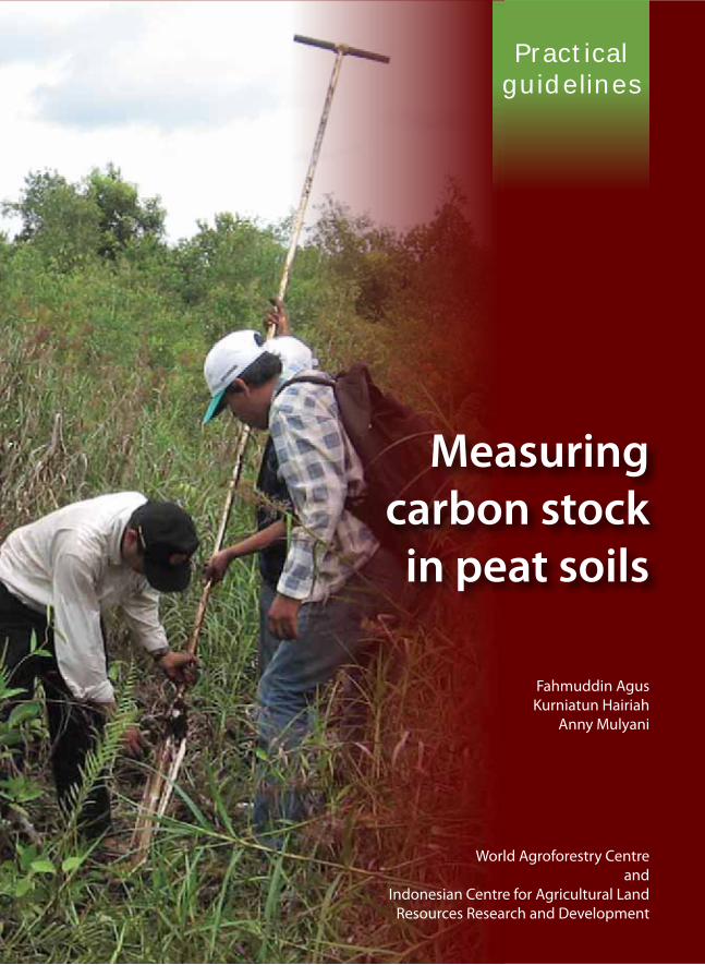
Cover photographs
Training in peat soil sampling in South Kalimantan, Indonesia. Photo credits: Harti Ningsih (front), ALLREDDI
project (back)
Design and layout
Tikah Atikah ([email protected]) and Sadewa ([email protected])
Copyediting
Robert Finlayson
iii
Figures v
Table vii
Glossary ix
Foreword xiii
1. Background 1
1.1. Difference between peat and mineral soils 2
1.2. Carbon emissions from Indonesian peatlands 4
2. Carbon-stock-related peat properties 9
2.1. Bulk density 9
2.2. Soil carbon content 10
2.3. Peat maturity 11
3. Carbon stock determination of peat soil 15
3.1. Determination of sampling points 15
3.2. Peat soil sampling 19
3.2.1. The kinds of peat samples 19
3.2.2. Peat sampling using peat auger 20
3.2.3. Procedure for peat sampling 22
3.2.4. Undisturbed soil sampling using soil core 26
3.2.5. Soil sampling using hollow box of galvanized iron sheet 27
3.3. Measurement of bulk density and organic matter content 29
3.3.1. Bulk density 29
3.3.2. Soil organic carbon content 31
4. Estimation of greenhouse gas emissions 43
5. Discussion 51
References 55
Appendix. Record sheet for peat observation 59
Contents

v
Figure 1. Schematic process of the formation and development of
peat in a wetland basin landscape 3
Figure 2. Schematic diagram of sampling points within a peat dome
using the grid or transects methods 17
Figure 3. Peat thickness maps 18
Figure 4. Observation plots of biomass and necromass
(Hairiah et al. 2011a) and peat sampling point placement 18
Figure 6. The peat auger 21
Figure 7. Using the peat auger on inundated peat 22
Figure 8. Peat sample appearing from the gouge on the fin’s surface 23
Figure 9. Peat samples 24
Figure 10. Soil core (soil ring) for undisturbed soil sampling 27
Figure 11. Stages of undisturbed soil sampling using soil core 27
Figure 12. Cubical and fluid peat samples 28
Figure 13. Illustration of peat soil volume 30
Figure 14. Porcelain mortar and pestle 32
Figure 15. Porcelain cups inside a furnace 33
Figure 16. Determination of peat maturity in the field 38
Figure 17. 10 ml syringe (left) and a sieve (right) 38
Figures
vi
Figure 18. Infra-Red Gas Analyzer (IRGA) and the closed chamber for
measuring CO2 gas flux emitted from the soil 46
Figure 19. Gas sampling from a closed chamber for gas concentration
measurement using gas chromatography 47
Figure 20. The rate of subsidence of drained peat as a function of time since
the drainage starts (Wösten et al. 1997) 49
vii
Table 1. Some differences in the characteristics of peat and upland soils 4
Table 2. Mean and standard deviation of selected peat properties
based on samples from Sumatra and Kalimantan 35
Table 3. Example of calculation of carbon stocks in peat soil from one
point of observation 36
Table 4. Indicators used for differentiating peat maturity in the field
and in the laboratory 37
Table 5. Calculation of the change in peat carbon stocks based on
bulk density (BD) and organic carbon content (Corg
) data
by layer 49
Tables

ix
Glossary
Aboveground biomass. Biomass above ground level (above the soil
surface), consisting of trees, other plants and animals (the latter are
normally considered to be negligible).
Belowground biomass. Biomass below the soil surface, consisting of plant
roots and soil biota.
Biomass. The total mass of living matter—plants and animals—in a unit
area. It is normally quantified on the basis of dry weight and usually
expressed in tonne per hectare (t/ha) or megagram per hectare (Mg/
ha). 1 Mg = 1 t = 1,000,000 gram.
Carbon pool. A subsystem that can store or release carbon. Examples of
carbon pools are plant biomass, necromass, soil and water.
Carbon budget. The balance of the transfer, during a specified time period,
of carbon from one carbon pool to another in a carbon cycle, or from
carbon pools to the atmosphere.
Carbon dioxide equivalent (CO2eq). A measure used to compare the
global warming potential (GWP) of certain greenhouse gases
relative to the warming potential of CO2; it combines differences in
the heat-trapping effect as well as expected residence time in the
atmosphere. For example, the GWP of methane (CH4) during an
accounting period of 100 years is 25 and for nitrous oxide (N2O) it is
298. This means that emissions of 1 t of CH4 and N
2O are equivalent
to 25 and 298 t of CO2, respectively.
Carbon dioxide. This is an odourless and colourless gas, expressed in the
formula CO2, that is formed from a variety of processes such as
combustion and/or decomposition of organic matter and volcanic
x
eruptions. It is captured from the atmosphere, along with solar
energy, by green plants through photosynthesis, and reemitted
by respiration, releasing energy. Today’s CO2 concentration in the
atmosphere is about 0.039% by volume or 388 mole ppm. The CO2
concentration has increased over the past century owing to the use
of fossil fuel and natural gas as well as the reduction of above- and
belowground terrestrial carbon stocks. The molecular weight of CO2
is 44 g; the atomic weight of carbon (C) is 12 g. Conversion of the
weight of C to CO2 is 44/12 or 3.67.
Carbon sequestration. The process of absorption of CO2 from the
atmosphere into plant tissues and soil.
Carbon stock. The mass of carbon stored in an ecosystem at any given time,
either in the form of biomass, necromass (dead organisms) or soil
carbon.
Carbon. Non-metallic chemical element expressed with the atomic symbol
‘C’, which is widely available in all organic (C bound to H and O) and
inorganic (elemental C) matter. Carbon has the atomic number 6 and
typical atomic weight of 12 g/mol, but a stable C13 and radioactive
C14 also occur in small amounts.
Emissions. The process of releasing greenhouse gases into the atmosphere.
Fibric. Early stage of peat decomposition where recognizable plant fibres
dominate (Table 4).
Forest. A vegetation (land-cover) type dominated by trees, which is
recognized through various definitions that, for example, restrict
the minimum area, give the minimum crown cover in current or
potential stages and express restrictions on the type of woody
vegetation that is included in the concept of ‘trees’.
Flux. The flow (of greenhouse gases) between pools, for example, from the
soil into the atmosphere in the unit weight of gas per unit surface
area, expressed as, for example, mg/(m2 hour).
Hemic. Intermediate stage of peat decomposition, between fibric and sapric
(Table 4).
xi
Histosol. Peat soil.
Land cover. The vegetation on the Earth’s surface, such as forests, half-open
woodlands, grasslands and open fields.
Land use. This term refers to the classification of land-cover types based on
human activities, such as plantation forestry, tree crops, field crops,
urban and conservation areas (please note that a term such as ‘forest’
can refer to both land cover and land use, depending on context).
Necromass (dead organic matter). The weight of dead organisms (mostly
plants) in a unit land area, usually expressed as dry weight in t/ha or
Mg/ha. Aboveground necromass includes dead trees (standing or on
the surface), the litter layer of dead leaves, twigs and branches and
crop residues. Belowground necromass includes dead roots and crop
residues buried by soil tillage that have not yet been converted into
soil organic matter.
Organic matter. Material derived from living matter that can decompose
or be the result of decomposition or materials consisting of organic
compounds.
Peat (as substrate). Soil dominated by partially decomposed plant residues,
with an organic C content of more than 18% (organic matter content
of more than 30%).
Peat soil (as soil type). Soils with at least 50 cm of peat. Peat soil has a
thickness ranging from 0.5 m (by definition) to more than 15 m.
Large areas of tropical peats have thicknesses ranging 2–8 m.
Peatland (as ecosystem). A land system dominated by peat soils. Peatland
is usually found in wetland conditions but not all wetlands are
peatlands. Mosses, grasses, shrubs and trees can contribute to the
formation of peat in water-saturated conditions, with the term ‘bog’
reserved for peatland dominated by moss.
Sapric. Advanced stage of peat decomposition into organic-matter-rich
‘earth’ without visible fibres (Table 4).
xii
Soil bulk density (BD). Dry weight of soil per unit volume (including
volume of soil solids and pores filled with gas and water).
Soil organic carbon content (Corg
). The mass of carbon per unit weight
of soil. Its units are percentage by weight or gram per kilogram
(g organic C/kg soil), tonne per tonne (t /t) or megagram per
megagram (Mg/Mg). If laboratory analysis only provides data on
organic matter content (for example, by the method of loss on
ignition (LOI)), the Corg content of the soil is normally assumed
to be 1/1.724 of soil organic matter content. If the peat soil has an
organic matter content of 98% then the Corg
= 98%/1.724 = 57% =
570 g/kg = 0.57 Mg/Mg = 0.57 t/t or simply 0.57.
Soil organic matter content. The mass of soil organic matter per unit
weight of dry soil. Usually expressed as percentage by weight
or gram per kilogram (g organic matter/kg dry soil) tonne per
tonne (t /t) or megagram per megagram (Mg/Mg). Organic matter
content of 98% by weight = 980 g/kg = 0.98 Mg/Mg = 0.98 t/t.
xiii
Peatland is one of the largest terrestrial carbon storehouses. However,
the carbon it contains is only protected from decomposition by the wet
conditions of the peat. Under special conditions where decomposition
is slow owing to low oxygen supply (water saturated), low nutrient
concentrations, and acidity, dead organic matter from trees or other
vegetation can start to pile up and accumulate, creating conditions
that further slow decomposition. Specialized trees, sedges and other
vegetation start to dominate and a peat swamp forest is formed. When
this starts to hold enough water, it can become a semi-autonomous
landscape unit, depending on rainfall and atmospheric nutrient inputs,
independent of the mineral soil and groundwater. The belowground
carbon stocks can reach 10–100 times those of the most lush tropical
forest. However, when the forest is cleared and the peat is drained the
stored carbon is readily decomposed and released as CO2, the most
important greenhouse gas. In addition, excessive drainage of peatland
increases its vulnerability to fires and, in turn, the peat loses its function
of buffering the surrounding environment from drought by the gradual
release of water stored in the peat ‘dome’. What took thousands of years
to accumulate can be burnt within a few days and decompose in a few
years or decades.
With the increase of human populations, land resources are becoming
scarcer. Peatlands that were once formerly regarded as wasteland are
increasingly being developed for various economic purposes such
as agriculture and settlements. As a consequence, the carbon sink of
actively growing peat becomes one of the most important carbon
sources associated with land uses, land-use changes and forestry.
Tropical peat alone is estimated to contribute 1–3% of global CO2
emissions owing to human activity. In Indonesia, the country that has
Foreword
xiv
the largest area of tropical peat, emissions from peatland are around
one-third of the total, although the exact numbers are debated and
uncertain. Therefore, in the context of Nationally Appropriate Mitigation
Actions (NAMAs) and efforts to Reduce Emissions from Deforestation
and Degradation (REDD+), conservation and sustainable management of
peatland has become one of the main concerns.
One of the requirements of any scheme to reduce carbon emissions
through REDD+ and NAMA is a credible monitoring, reporting and
verifying (MRV) system. MRV systems document, report on and verify
changes in carbon stocks in a transparent, consistent and accurate
manner. An MRV system must be supported by a reliable method
for measuring carbon stocks and changes in them, both above- and
belowground. This booklet provides practical guidance on peat sampling
and analysis, calculation of the amount of carbon and data interpretation.
It also explains the relationship between changes in carbon stock and CO2
emissions.
We thank the various people and organizations who have assisted in
writing and publishing this book. Hopefully, it will be useful for people
who are engaged in the MRV of carbon stocks in peatland.
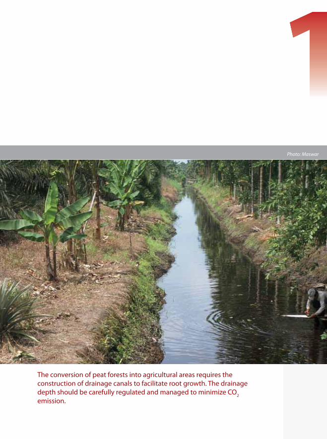
The conversion of peat forests into agricultural areas requires the
construction of drainage canals to facilitate root growth. The drainage
depth should be carefully regulated and managed to minimize CO2
emission.
Photo: Maswar

1
Background
Soil is one of the three carbon pools on land. Other pools include biomass
and necromass (IPCC 2006). Carbon stocks in natural forestland around the
world have been estimated to total about 1146 gigatonne (Gt). The world’s
peatlands are thought to contain 180 to 455 Gt C on only a fraction of the
total land area. The carbon stocks in natural forests in the tropical parts of
Asia are larger than in sub-tropical regions, with an average range of 41–54
Gt C aboveground and about 43 Gt in the soil or an average range of 132–
174 t/ha in plant biomass and 139 t/ha in the soil (Dixon et al. 1994).
Indonesia and several other countries in tropical regions, particularly
Malaysia, Papua New Guinea and Brunei Darussalam, as well as having
mineral soils also have peat soils (Histosols). Peat soils store much more
carbon per unit area than mineral soils. The amount could be more than ten
times the carbon stored in upland (mineral) soils, depending on the peat
thickness.
Peatlands store carbon in plant biomass and necromass (above the surface
and in the soil). In the soil, the carbon is stored in peat layers and in the
elevated carbon content of the mineral soil layer below the peat layer
(substratum). Of the various carbon stores, the largest stock in peatland is
in the peat soil itself, followed by the plant biomass. In uplands, the carbon
stored in plant biomass can exceed the carbon stored in the soil, depending
on the type and density of crops covering the land (Hairiah and Rahayu
2010).
The concentration of carbon in peat soils ranges 30–70 kg/m3 (or 30–70 g/
dm3), which is equivalent to 30–700 t/ha/m of peat depth. Thus, if a peat
soil has a thickness of 10 m, then the carbon stock in it is likely to be around
3000–7000 t/ha (Agus and Subiksa 2008). In upland conditions, carbon stock
in the 0–100 cm soil layer ranged 20–300 t/ha (Shofiyati et al. 2010) but at
a depth of more than 100 cm the amount of carbon stored is so low that it
Agus et al. (2011)
2
usually can be ignored. Peat thickness varied from 0.5 m to deeper than 15
m but the commonly found thickness was 2–8 m.
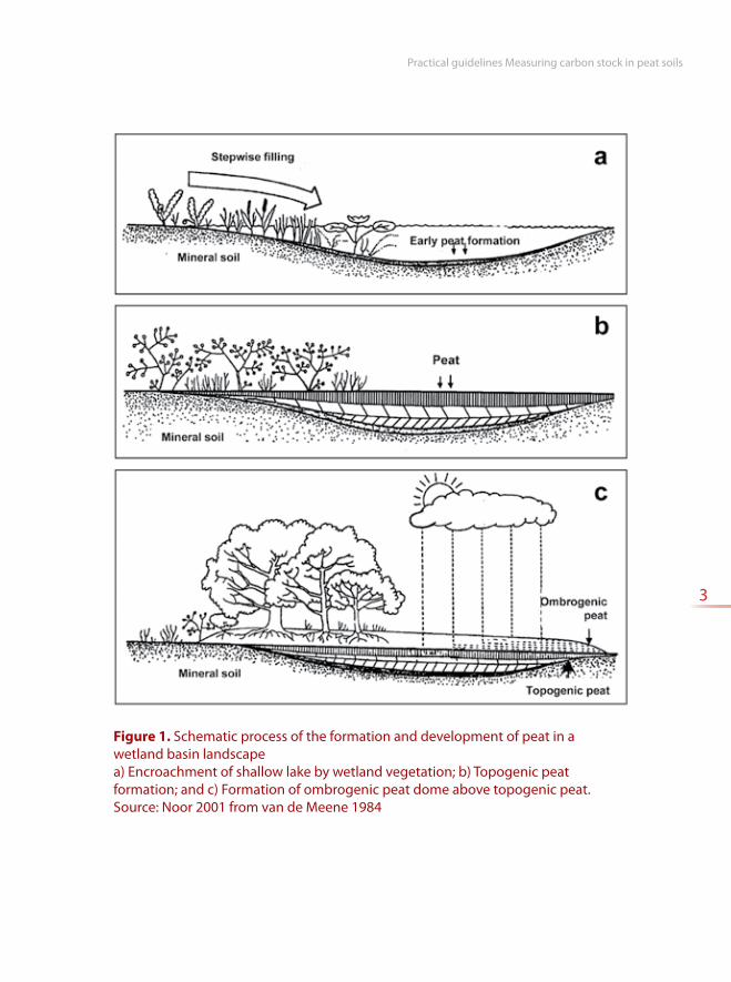
Formation of peatland often starts in a basin or shallow lake that gradually
fills with organic material from dead plants. On further expansion the
peatland may form a ‘peat dome’. The edges of the dome tend to be thinner
with less carbon stock whereas the central parts tend to be thicker and
contain more carbon stock (Figure 1). However, this situation does not
apply to all areas of peat. Often the relief of the bottom of the peat is not
flat, but bumpy. Furthermore, not all landscapes of peat form a dome.
Occasionally, peat formation ceases before a dome is formed, for example,
owing to the influence of drainage and land clearing. Other peat areas
develop in former river beds and the subsoil may still have traces of the
meandering river, with a correspondingly high variability of peat depth,
even though the surface appears to be even.
At the micro-spatial level, soil carbon content in the peat varies both
vertically and horizontally. Linked to the process of peat formation there
may be voids with very low bulk density that become covered. But next
to such a void there may be dead trees that have not completely decayed
and have high carbon density. This variation is a source of uncertainty
in measuring peat carbon stock and a challenge. For example, if we are
attempting to take samples using an auger and encounter dead wood we
must abandon the place for one nearby, which may introduce a bias in the
results.
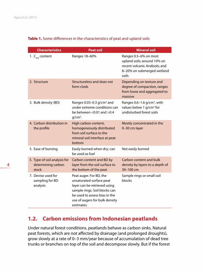
1.1. Difference between peat and mineral soils
Peat soils differ from mineral soils in Corg
content, structure, bulk density,
distribution of carbon in the soil profile and the ease of burning and oxidation
(Table 1). Therefore, the tools used for soil sampling and the soil depths that
are sampled are also different between the two soil types.
Practical guidelines Measuring carbon stock in peat soils
3
Figure 1. Schematic process of the formation and development of peat in a
wetland basin landscape
a) Encroachment of shallow lake by wetland vegetation; b) Topogenic peat
formation; and c) Formation of ombrogenic peat dome above topogenic peat.
Source: Noor 2001 from van de Meene 1984
Agus et al. (2011)
4
Table 1. Some differences in the characteristics of peat and upland soils
Characteristics Peat soil Mineral soil
1. Corg
content Ranges 18–60% Ranges 0.5–6% on most
upland soils; around 10% on
recent volcanic Andisols; and
8–20% on submerged wetland
soils
2. Structure Structureless and does not
form clods
Depending on texture and
degree of compaction, ranges
from loose and aggregated to
massive
3. Bulk density (BD) Ranges 0.03–0.3 g/cm3 and
under extreme conditions can
be between <0.01 and >0.4
g/cm3.
Ranges 0.6–1.6 g/cm3, with
values below 1 g/cm3 for
undisturbed forest soils
4. Carbon distribution in
the profile
High carbon content,
homogeneously distributed
from soil surface to the
mineral soil interface at peat
bottom
Mostly concentrated in the
0–30 cm layer
5. Ease of burning Easily burned when dry; can
be used as fuel
Not easily burned
5. Type of soil analysis for
determining carbon
stock
Carbon content and BD by
layer from the soil surface to
the bottom of the peat
Carbon content and bulk
density by layers to a depth of
30–100 cm
7. Devise used for
sampling for BD
analysis
Peat auger. For BD, the
unsaturated surface peat
layer can be retrieved using
sample rings. Soil blocks can
be used to assess bias in the
use of augers for bulk density
estimates
Sample rings or small soil
blocks
1.2. Carbon emissions from Indonesian peatlands
Under natural forest conditions, peatlands behave as carbon sinks. Natural
peat forests, which are not affected by drainage (and prolonged droughts),
grow slowly at a rate of 0–3 mm/year because of accumulation of dead tree
trunks or branches on top of the soil and decompose slowly. But if the forest
Practical guidelines Measuring carbon stock in peat soils
5
is cleared and drained, the peatland changes from a sink to a CO2 source.
There are several factors that can alter the function of peatland from a sink
into a CO2 source.
1. Land clearing that increases the amount of sunlight onto the peat surface
so that soil temperature and the activity of decomposing microorganisms
increase. Felling of trees also increases the availability of fresh organic
matter that easily decomposes into CO2 under aerobic, and CH
4 under
anaerobic, conditions. Thus, in addition to emissions from tree biomass,
logging also accelerates decomposition of organic matter.
2. Drainage that decreases the peat watertable on the site and surrounding
areas that are under agricultural and forest covers. Drainage changes the
soil conditions from anaerobic (water saturated) to aerobic (unsaturated)
and increases CO2 emissions. Recession of the watertable can also occur
naturally, such as under the influence of drought, but a high watertable
dominates humid areas where peat is formed.
3. Peat fires. Fires increase CO2 emissions owing to burning or oxidation
of one or a combination of plant biomass, necromass and peat layers.
Fires often occur during land-use change from forest to agriculture or
other land uses. Fires can also occur during long drought periods. Under
traditional farming practices, burning can be done intentionally to reduce
soil acidity and improve soil fertility. But, on the other hand, this practice
increases the contribution of peat to CO2 emissions.
4. The addition of fertilizers and ameliorants. The addition of fertilizers, such
as nitrogen fertilizers, lowers the ratio of soil C/N and encourages the
decomposition of organic matter by microorganisms, followed by the
release of CO2. Nitrogen fertilizer can also contribute to N
2O emission.
Fertilizing with manure or the addition of ameliorants that increase the
pH of peat can also accelerate peat decomposition.
Indonesia has about 15 million ha of peatland with belowground carbon
stock of about 20-30 Gt. This is a revision of earlier peatland map by
Wahyunto et al. 2004, 2005, 2006 using soil survey data. However, with
increasing population and the demands of economic development, the
exploitation of peat for various development purposes has also increased
so that the amount of CO2 emissions from peatlands is increasing. It has
been estimated that CO2 emissions from peat and related forest land uses
Agus et al. (2011)
6
and land-use changes is more than 50% of the total emissions of Indonesia
(Hooijer et al. 2010, Boer et al. 2010).
The Reducing Emissions from Deforestation and Forest Degradation (REDD)
schemes currently in testing phases require that the carbon balance is
measureable, reportable and verifiable according to international standards.
This booklet provides a step-by-step guide to measurement of carbon stocks
in peat soils, including examples of carbon stocks and emissions calculations.
The last chapter describes the relationship between carbon stocks and CO2
emissions from peat soils.
The measurement of carbon stocks in peatland as described in this booklet
is supplementary to the carbon stock measurement technique according
to the Rapid Carbon Stock Appraisal method developed by the World
Agroforestry Centre Southeast Asia Regional Program (Hairiah and Rahayu
2007), with a focus on measurement at field level and its extrapolation to
landscape level (Hairiah et al. 2011a, b).
7
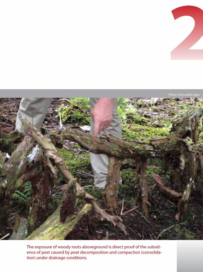
The exposure of woody roots aboveground is direct proof of the subsid-
ence of peat caused by peat decomposition and compaction (consolida-
tion) under drainage conditions.
Photo: Fahmuddin Agus

9
Carbon-stock-related
peat properties
The main data needed to calculate carbon stocks in a peat landscape are:
Bulk Density (BD), [g/cm3 or kg/dm3 or t/m3]
Organic carbon content (Corg
), [% by weight or g/g or kg/kg]
Peat thickness. If the samples consist of many layers, the thickness of each
layer with its respective BD and Corg
, needs to be measured [cm or m]
Area of land in which the carbon stock is to be estimated [ha or km2]
In addition to the above data, additional information on peat maturity or
fibre content will be helpful.
2.1. Bulk density
Bulk density (BD) is the mass of soil solid phase (Ms) divided by the total
soil volume (Vt). The total volume of soil is the sum of the volume of soil
solid phase and the volume of soil pores (air filled and water filled) in an
undisturbed (as in the field) condition. The BD determination of peat soils in
principle is the same as that of mineral soils (see Chapter 2.4.2. in Hairiah et
al. 2011a), but the sampling and handling procedures are different because
of the different properties of the two types of soils.
Ms is determined from oven dry weight at 105 oC for 48 hours or more,
until constant weight is achieved (no reduction in sample weight when
the samples are dried for a longer time). Often the samples taken from the
field are very wet and when a sub-sample is taken for drying it tends to
cause substantial errors in the BD measurement. For that reason, usually the
whole sample taken with a peat auger is quantitatively transferred into an
aluminium can for drying at 105 oC for 48–96 hours to reach the constant
weight.
Agus et al. (2011)
10
BD values of peat soils generally range between 0.03 and 0.3 g/cm3. However,
within a peat profile, sometimes pockets may exist which are nearly empty of
peat and filled with water, with a BD of < 0.01 g/cm3. This condition is often
found in natural peat forests. By contrast, the BD of a peat surface layer under
several years of agricultural use may increase to as high as 0.3 to 0.4 g/cm3.
BD is determined in the laboratory by a gravimetric method of weighing
the oven dry weight of a known volume of peat. The samples used for the
analysis may be samples taken using a peat auger (Ejkelkamp model), ring
sample or cubical sample as long as the sample volume can be determined
easily.
According to Maswar (2011), division by a correction factor of 1.136 is
needed to correct for compaction that occurs at the sampling stage. This
correction factor was established by comparison of auger samples and large
blocks of peat obtained from soil pits and is considered to represent the real
condition in the field.
2.2. Soil carbon content
The organic carbon content of soil can be determined by one of several
methods, namely, dry combustion (loss on ignition (LOI)), Walkley and Black
procedure (1934) or CN auto-analyzer. For peat soil, the CN autoanalyzer
or LOI techniques are more preferable than the Walkley and Black. The LOI
method is relatively simple but nevertheless gives a fairly accurate figure for
determining the ash content (inorganic material) and peat organic matter
because with this method the soil organic matter can be burned completely.
However, LOI technique semi-quantitatively estimate peat carbon content
by multiplying peat organic matter content with a constant of 0.58. On the
other hand, under the Walkley and Black technique, there is a possibility
of incomplete digestion of organic matter, leading to underestimating the
carbon content value. The CN autoanalyzer is a direct method (measuring
carbon or CO2), however, the amount of sample analyzed is very small (a
few milligram), such that ensuring the representativeness of the sample is
critical and duplicate measurements are needed. In this booklet, we limit
explanation to the LOI technique only , although for the quantitative analysis
the CN auto-analyzer technique is preferable.
Practical guidelines Measuring carbon stock in peat soils
11
2.3. Peat maturity
Peat maturity observation is useful for assessing peat fertility and carbon
content. The more mature the peat, the generally more fertile, although
many other factors also determine fertility, including clay or ash mixture. The
more mature peats also tend to have a higher carbon content per volume.
Observation of peat maturity can be done in the field or in the laboratory
based on fibre content, which will be discussed in the next section.

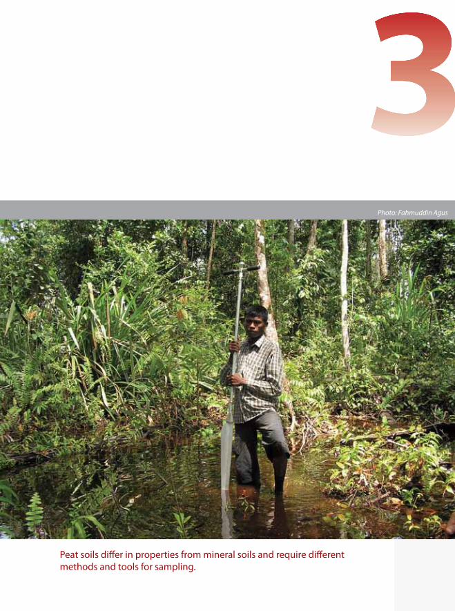
Peat soils differ in properties from mineral soils and require different
methods and tools for sampling.
Photo: Fahmuddin Agus

15
Measurement of carbon stocks in a landscape or peat dome consists of three
stages.
1. Determination of sampling points
2. Peat soil sampling
3. Analysis of samples and calculation of carbon stocks
3.1. Determination of sampling points
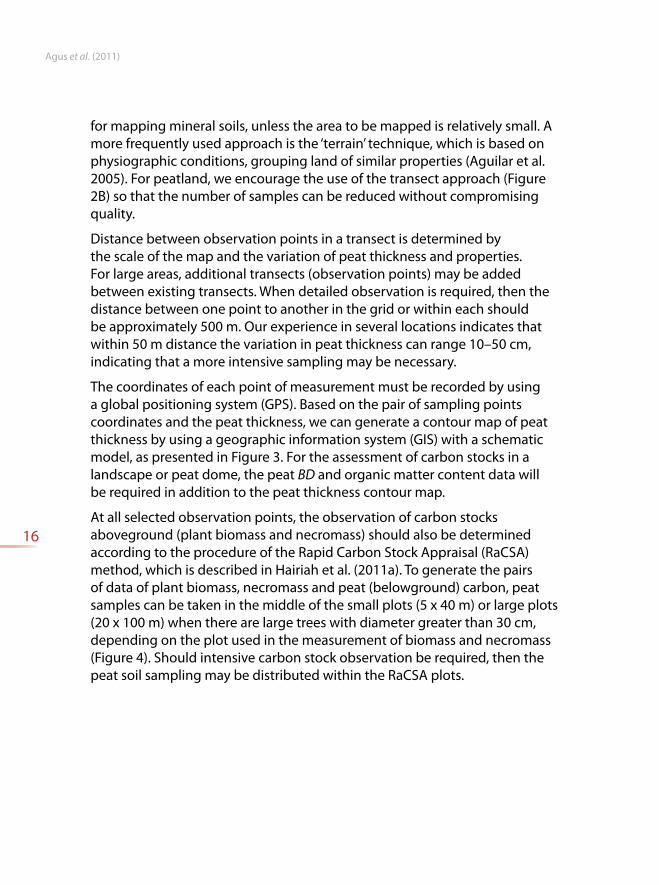
For mapping the carbon stocks in a landscape or dome, the points of
sampling may be according to ‘grid’ or from multiple transects across the
peat dome, for example, north–south, east–west, northeast–southwest and
northwest–southeast so that a range of peat thicknesses will be represented.
Usually, the peat tends to be thicker closer to the centre of a dome. However,
the surface of the underlying mineral soil at the bottom of the peat is
usually irregular, tending to be bumpy. The more irregular the surface of the
underlying mineral substratum the higher the variation of thickness and
carbon stocks. This requires a more intensive sampling.
Figure 2 shows the two approaches to determine sampling points.
Sampling using the grid system requires more observation points. The
number of observation points and the total area represented by each grid is
determined by the scale of the map or the level of accuracy required in the
measurement. For the mapping scales of 1:10 000, 1:25 000, 1:50 000 and
1:250 000 an ideal sampling intensity is one sampling point for 1 ha, 6.25 ha,
25 ha and 625 ha, respectively. However, this approach will require a very
high number of soil samples. This method is less popular nowadays, even
Carbon stock
determination of peat soil
Agus et al. (2011)
16
for mapping mineral soils, unless the area to be mapped is relatively small. A
more frequently used approach is the ‘terrain’ technique, which is based on
physiographic conditions, grouping land of similar properties (Aguilar et al.
2005). For peatland, we encourage the use of the transect approach (Figure
2B) so that the number of samples can be reduced without compromising
quality.
Distance between observation points in a transect is determined by
the scale of the map and the variation of peat thickness and properties.
For large areas, additional transects (observation points) may be added
between existing transects. When detailed observation is required, then the
distance between one point to another in the grid or within each should
be approximately 500 m. Our experience in several locations indicates that
within 50 m distance the variation in peat thickness can range 10–50 cm,
indicating that a more intensive sampling may be necessary.
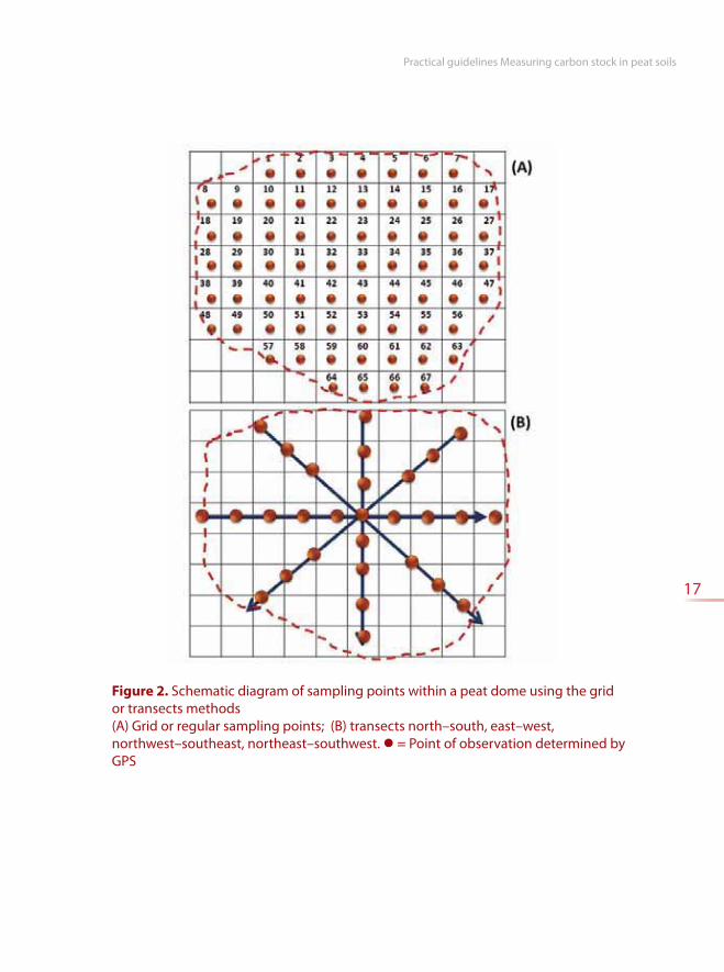
The coordinates of each point of measurement must be recorded by using
a global positioning system (GPS). Based on the pair of sampling points
coordinates and the peat thickness, we can generate a contour map of peat
thickness by using a geographic information system (GIS) with a schematic
model, as presented in Figure 3. For the assessment of carbon stocks in a
landscape or peat dome, the peat BD and organic matter content data will
be required in addition to the peat thickness contour map.
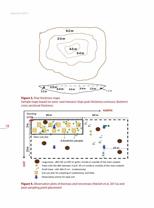
At all selected observation points, the observation of carbon stocks
aboveground (plant biomass and necromass) should also be determined
according to the procedure of the Rapid Carbon Stock Appraisal (RaCSA)
method, which is described in Hairiah et al. (2011a). To generate the pairs
of data of plant biomass, necromass and peat (belowground) carbon, peat
samples can be taken in the middle of the small plots (5 x 40 m) or large plots
(20 x 100 m) when there are large trees with diameter greater than 30 cm,
depending on the plot used in the measurement of biomass and necromass
(Figure 4). Should intensive carbon stock observation be required, then the
peat soil sampling may be distributed within the RaCSA plots.
Practical guidelines Measuring carbon stock in peat soils
17
Figure 2. Schematic diagram of sampling points within a peat dome using the grid
or transects methods
(A) Grid or regular sampling points; (B) transects north–south, east–west,
northwest–southeast, northeast–southwest. = Point of observation determined by
GPS
Agus et al. (2011)
18
0-2 m
2-3 m
3-4 m4-5 m
2-3 m3-4 m4-5 m1-2 m
2-3 m3-4 m
1-2 m
Figure 4. Observation plots of biomass and necromass (Hairiah et al. 2011a) and
peat sampling point placement
Figure 3. Peat thickness maps
Sample maps based on west–east transect: (top) peat thickness contours; (bottom)
cross-sectional thickness
Practical guidelines Measuring carbon stock in peat soils
19
3.2. Peat soil sampling
3.2.1. The kinds of peat samples
In general, soil samples taken in the field can be divided into two kinds,
that is, intact (undisturbed) and disturbed soil samples.
Undisturbed soil samples are those which structure is similar to the actual
structure of the peat in the field. Disturbed soil samples are those which
structure is different from the original structure because of disturbance
during sampling, handling and transportation. (Nearly) undisturbed soil
samples can be obtained using a peat auger or soil core (hollow tube,
which is also known as ‘soil rings’). Disturbed soil samples can be taken
with a regular soil auger, hoe, shovel or machete.
For peat sampling, the use of peat auger is recommended (Figure 5, left)
because it can be used to sample almost undisturbed soil from the top to
bottom layers. A peat auger can be used even under inundated conditions.
Samples taken by a peat auger can be used for the analysis of bulk density,
water content (% volume) and chemical properties including the carbon
content.
Soil cores can be used for sampling the mature surface layer of peat under
unsaturated condition. Soil cores cannot be used for fibric (immature) peat
or when the peat is saturated. As with the use of soil cores, cube-shaped
samples can only be taken for the surface layer of mature (sapric maturity)
unsaturated peat.
Agus et al. (2011)
20
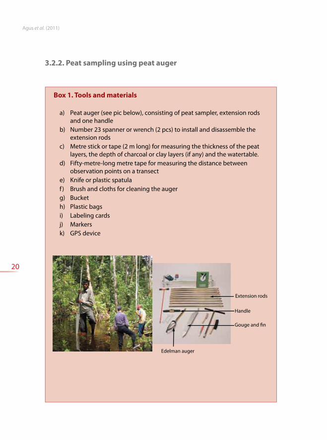
Box 1. Tools and materials
a) Peat auger (see pic below), consisting of peat sampler, extension rods
and one handle
b) Number 23 spanner or wrench (2 pcs) to install and disassemble the
extension rods
c) Metre stick or tape (2 m long) for measuring the thickness of the peat
layers, the depth of charcoal or clay layers (if any) and the watertable.
d) Fifty-metre-long metre tape for measuring the distance between
observation points on a transect
e) Knife or plastic spatula
f ) Brush and cloths for cleaning the auger
g) Bucket
h) Plastic bags
i) Labeling cards
j) Markers
k) GPS device
Extension rods
Gouge and fin
Edelman auger
Handle
3.2.2. Peat sampling using peat auger
Practical guidelines Measuring carbon stock in peat soils
21
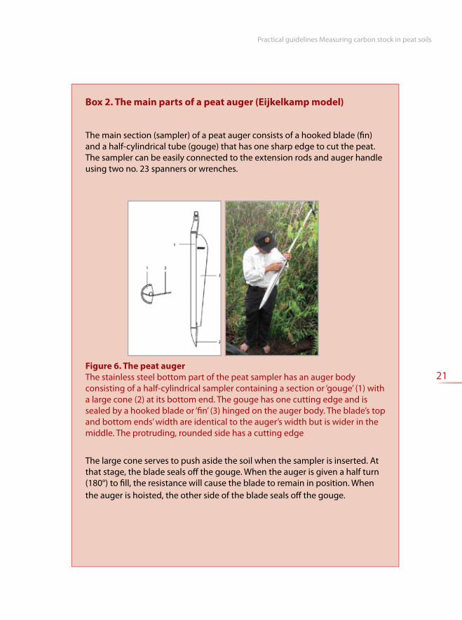
Box 2. The main parts of a peat auger (Eijkelkamp model)
The main section (sampler) of a peat auger consists of a hooked blade (fin)
and a half-cylindrical tube (gouge) that has one sharp edge to cut the peat.
The sampler can be easily connected to the extension rods and auger handle
using two no. 23 spanners or wrenches.
Figure 6. The peat auger
The stainless steel bottom part of the peat sampler has an auger body
consisting of a half-cylindrical sampler containing a section or ‘gouge’ (1) with
a large cone (2) at its bottom end. The gouge has one cutting edge and is
sealed by a hooked blade or ‘fin’ (3) hinged on the auger body. The blade’s top
and bottom ends’ width are identical to the auger’s width but is wider in the
middle. The protruding, rounded side has a cutting edge
The large cone serves to push aside the soil when the sampler is inserted. At
that stage, the blade seals off the gouge. When the auger is given a half turn
(180°) to fill, the resistance will cause the blade to remain in position. When
the auger is hoisted, the other side of the blade seals off the gouge.
Agus et al. (2011)
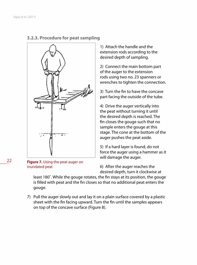
22
1) Attach the handle and the
extension rods according to the
desired depth of sampling.
2) Connect the main bottom part
of the auger to the extension
rods using two no. 23 spanners or
wrenches to tighten the connection.
3) Turn the fin to have the concave
part facing the outside of the tube.
4) Drive the auger vertically into
the peat without turning it until
the desired depth is reached. The
fin closes the gouge such that no
sample enters the gouge at this
stage. The cone at the bottom of the
auger pushes the peat aside.
5) If a hard layer is found, do not
force the auger using a hammer as it
will damage the auger.
6) After the auger reaches the
desired depth, turn it clockwise at
least 180˚. While the gouge rotates, the fin stays at its position, the gouge
is filled with peat and the fin closes so that no additional peat enters the
gouge.
7) Pull the auger slowly out and lay it on a plain surface covered by a plastic
sheet with the fin facing upward. Turn the fin until the samples appears
on top of the concave surface (Figure 8).
Figure 7. Using the peat auger on
inundated peat
3.2.3. Procedure for peat sampling
Practical guidelines Measuring carbon stock in peat soils
23
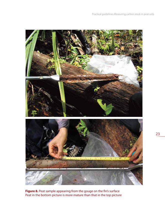
Figure 8. Peat sample appearing from the gouge on the fin’s surface
Peat in the bottom picture is more mature than that in the top picture
Agus et al. (2011)
24
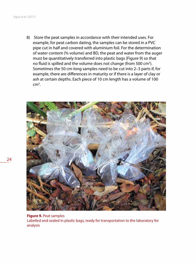
8) Store the peat samples in accordance with their intended uses. For
example, for peat carbon dating, the samples can be stored in a PVC
pipe cut in half and covered with aluminium foil. For the determination
of water content (% volume) and BD, the peat and water from the auger
must be quantitatively transferred into plastic bags (Figure 9) so that
no fluid is spilled and the volume does not change (from 500 cm3).
Sometimes the 50 cm-long samples need to be cut into 2–3 parts if, for
example, there are differences in maturity or if there is a layer of clay or
ash at certain depths. Each piece of 10 cm length has a volume of 100
cm3.
Figure 9. Peat samples
Labelled and sealed in plastic bags, ready for transportation to the laboratory for
analysis
Practical guidelines Measuring carbon stock in peat soils
25
Notes
depth so that the error in depth determination can be minimized.
needed. An auger set of nine extension rods can be used to take samples to a depth
of 10 m. Peat sampling to a depth of 400 cm is relatively easy to do but sampling at
deeper depth will be more difficult.
gouge may not be filled and the fin may not close properly. In such circumstances,
the augering needs to be repeated at another point nearby otherwise the volume
of sample will be < 500 cm3.
ordinary soil auger (Edelman auger) to penetrate hard layers above the intended
peat sampling depth.
that they were no longer suitable for bulk density determination.
Box 3. Maintenance of peat auger
The auger must be kept clean. After use, wash the auger with
fresh water.
Use a brush to clean the threads at each end of the extension
rods.
Dry the auger using a dry cloth and let it completely dry under
the sun.
Keep the auger in its bag or box.
Agus et al. (2011)
26
3.2.4. Undisturbed soil sampling using soil core
The method of peat sampling using soil cores is the same as for mineral soils.
However, only mature and relatively dry peat can be sampled using a soil
ring. Stages of sampling using the rings are shown in Figure 11 (modified
from Suganda et al. 2007).
1. Clean the soil surface of litter and small plants.
2. Dig a circle with a diameter of about 20 cm to a desired depth. For
example, to 5 cm if the sample is to be taken from a depth of 5–10 cm.
Trim the soil with a knife or a machete.
3. Put a ring on the ground vertically.
4. Put a small block of wood on the ring, press slowly until three-quarters of
the ring is inserted into the soil.
5. Put another ring on top of the first one, and press until about 1 cm of the
second ring is inserted in the soil.
6. Separate the upper ring from the bottom ring slowly.
7. Dig the ring using a shovel or a machete. In digging, the tip of the shovel
should be deeper than the lower end of the ring so that 1 or 2 cm of the
soil beneath the ring is lifted up.
8. Slice excess soil on top of the ring with caution and close the ring using
a plastic cap that attaches snugly to the ring. Then slice the excess soil at
the bottom of the ring and close it with another cap.
9. Attach a paper label to the cap of the ring that gives the sample’s location,
date of sampling and depth of sample.
Practical guidelines Measuring carbon stock in peat soils
27
3.2.5. Soil sampling using hollow box of galvanized iron sheet
Similar to sampling with a soil ring, this method is only applicable for
mature and dry peat. Alternatively, a peat cube can be created with a knife
or machete (Figure 12) without the use of soil core or soil sampling box. The
method of sampling with a metal box is similar to that using a soil ring. The
detail is described in Hairiah et al. (2011a).
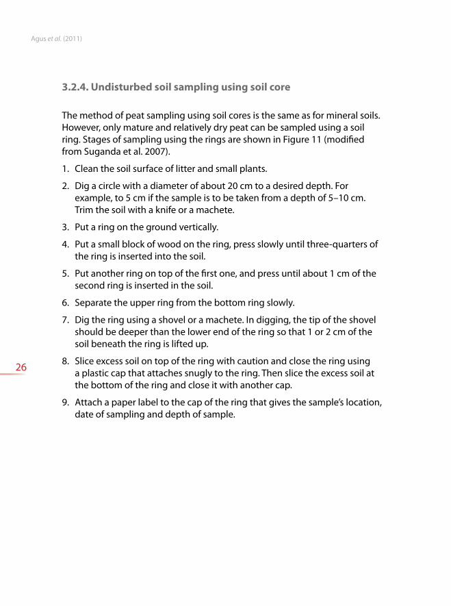
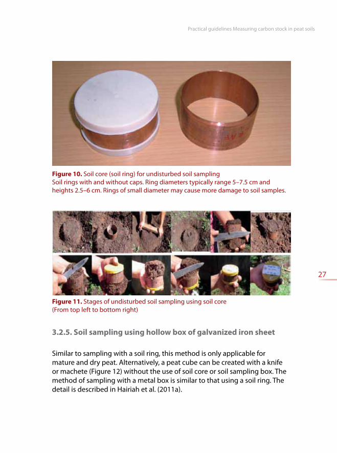
Figure 10. Soil core (soil ring) for undisturbed soil sampling
Soil rings with and without caps. Ring diameters typically range 5–7.5 cm and
heights 2.5–6 cm. Rings of small diameter may cause more damage to soil samples.
Figure 11. Stages of undisturbed soil sampling using soil core
(From top left to bottom right)
Agus et al. (2011)
28
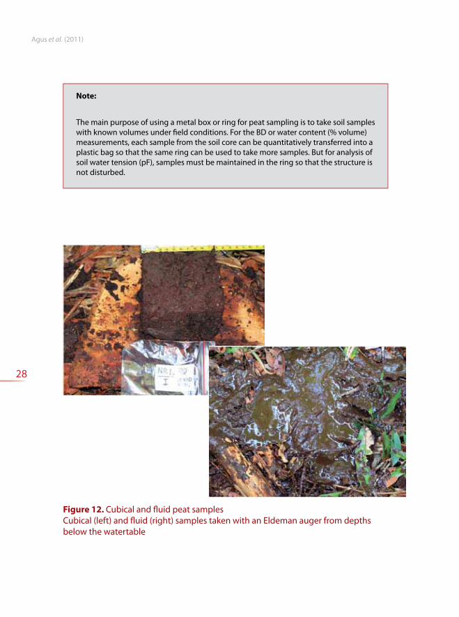
Figure 12. Cubical and fluid peat samples
Cubical (left) and fluid (right) samples taken with an Eldeman auger from depths
below the watertable
Note:
The main purpose of using a metal box or ring for peat sampling is to take soil samples
with known volumes under field conditions. For the BD or water content (% volume)
measurements, each sample from the soil core can be quantitatively transferred into a
plastic bag so that the same ring can be used to take more samples. But for analysis of
soil water tension (pF), samples must be maintained in the ring so that the structure is
not disturbed.
Practical guidelines Measuring carbon stock in peat soils
29
3.3. Measurement of bulk density and organic matter
content
For the determination of carbon stocks in peat soil the data of BD, Corg
, the
thickness of the peat and area of the landscape or dome are required.
3.3.1. Bulk density
Peat BD is determined in the laboratory by a gravimetric method. Samples
to be used for BD analysis can be taken using a peat auger (for example,
Ejkelkamp model), a soil core or hollow metal box, each with associated
sample volume. The method of soil sampling is as described above.
Determination of BD
1. Transfer each sample obtained with peat auger or ring quantitatively
into an aluminium cup. If using a soil core, each sample can either be
removed from the core or the core with sample inside can be placed in
an aluminium can for oven drying.
2. If the data of soil moisture content is required, then weigh the wet soil
inside the cup. The mass of wet soil (Mt) is M
w + M
s, where Ms is the mass
of the dry soil and Mw is the mass of water contained in the soil matrix
(Figure 13).
3. Dry the soil samples in an oven at 105 oC for 2 x 24 hours or until the
constant weight is achieved. If the sample is very wet, it may take 4–5 x
24 hours to reach the constant weight. The constant weight is obtained
when the sample weight does not decrease after subsequent drying.
For example, if the weight of sample that is dried for 2 x 24 hours is still
higher than the sample that was dried for 3 x 24 hours, then the drying
should be continued.
4. Put the dry soil within the aluminium can in a desiccator for about 10
minutes.
5. Weigh the dry weight of the soil (Ms) plus the can weight (M
c).
6. Save the soil samples for analysis of organic materials with the LOI
method. If the carbon content is to be determined by CN analyzer or
Walkley and Black method, the oven-dried soil samples cannot be used,
instead air dried samples must be used.

Agus et al. (2011)
30
Determine the volume of soil samples, Vt. If soil samples are taken with the
soil ring, then Vt = πr2t, where r is the inside radius and t is the height of
the ring. If the samples are from an Eijkelkamp peat auger with a thickness
(sample length) of 50 cm, then Vt = 0.5 dm3 = 500 cm3. If a 20 cm-long peat
sample was taken from the peat auger, then Vt= 200 cm3.
Calculate BD as
Vt = V
s + V
w + V
a
Figure 13. Illustration of peat soil volume
Peat soil volume consists of the volume of soil solids (Vs), liquid (V
w) and gas (V
a) and
the mass of soil solids (Ms), water (M
w) and air (M
a). The mass of soil solids, M
s, is the
sum of the mass of organic matter, Mom
, and ash Mash
DB [1]
Practical guidelines Measuring carbon stock in peat soils
31
If the unit weight is gram (g) and unit volume is cm3 then the unit for BD is g/
cm3. This unit is equivalent with kg/dm3 or t/m3.
Wash and dry the cans in the oven at 105 oC for 1 2 hours. Weigh each can,
Mc. Soil water content (by volume), KA
v, can be calculated as:
[2a]
Water content by weight, KAm
,
[2b]
Units used are cm3/cm3 and g/g to give an indication that the water content
was calculated based on volume and weight, respectively. The unit can be
written in the form of %.
The value of water content by volume (KAv) can be converted into water
content by weight (KAm
) with the formula:
KAm
= KAv * ρ
w/BD [3]
Where ρw
is water density which is approximately 1 g/cm3
3.3.2. Soil organic carbon content
Determination of soil organic matter content with the LOI method.
The mass of soil solids, Ms, as illustrated in Figure 13, consists of the mass of
organic matter, Mom
, and the mass of ash, Mash
. In the LOI method, all organic
matter present in the soil sample is burned at a temperature of 550 oC for 6
hours. The burned organic matter will evaporate and the remaining material
is inorganic matter such as clay, silt and other non-combustible substances
that are collectively called ash for the purpose of this analysis. The mass
lost from the sample equals the mass loss of organic matter. Conversion
of organic matter to organic carbon content uses the conversion factor of
1/1.724. This method is a semi-quantitative one, since the mass lost during
Agus et al. (2011)
32
the conversion reflects only the organic matter content and the conversion
factor of 1/1.724 is a generalized relationship between organic matter and
carbon content.
Procedure of LOI
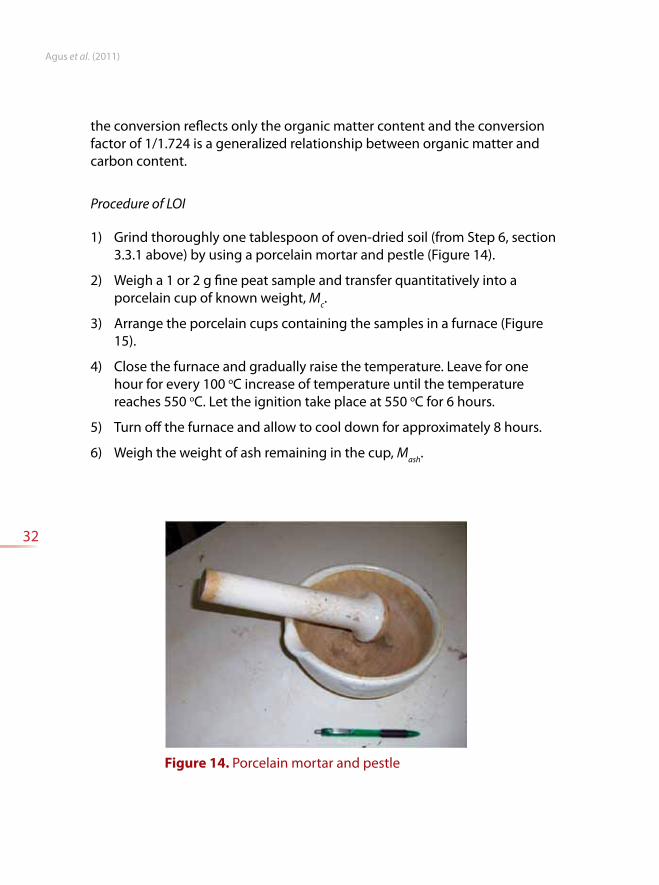
1) Grind thoroughly one tablespoon of oven-dried soil (from Step 6, section
3.3.1 above) by using a porcelain mortar and pestle (Figure 14).
2) Weigh a 1 or 2 g fine peat sample and transfer quantitatively into a
porcelain cup of known weight, Mc.
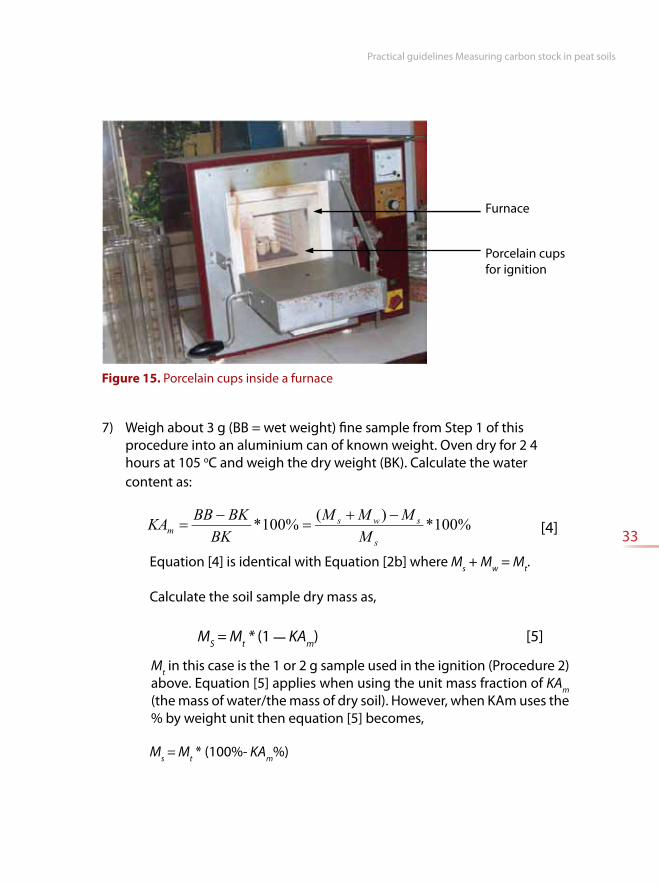
3) Arrange the porcelain cups containing the samples in a furnace (Figure
15).
4) Close the furnace and gradually raise the temperature. Leave for one
hour for every 100 oC increase of temperature until the temperature
reaches 550 oC. Let the ignition take place at 550 oC for 6 hours.
5) Turn off the furnace and allow to cool down for approximately 8 hours.
6) Weigh the weight of ash remaining in the cup, Mash
.
Figure 14. Porcelain mortar and pestle
Practical guidelines Measuring carbon stock in peat soils
33
7) Weigh about 3 g (BB = wet weight) fine sample from Step 1 of this
procedure into an aluminium can of known weight. Oven dry for 2 4
hours at 105 oC and weigh the dry weight (BK). Calculate the water
content as:
[4]
Equation [4] is identical with Equation [2b] where Ms + M
w = M
t.
Calculate the soil sample dry mass as,
MS = M
t * (1 — KA
m) [5]
Mt in this case is the 1 or 2 g sample used in the ignition (Procedure 2)
above. Equation [5] applies when using the unit mass fraction of KAm
(the mass of water/the mass of dry soil). However, when KAm uses the
% by weight unit then equation [5] becomes,
Ms = M
t * (100%- KA
m%)
Figure 15. Porcelain cups inside a furnace
Porcelain cups
for ignition
Furnace
Agus et al. (2011)
34
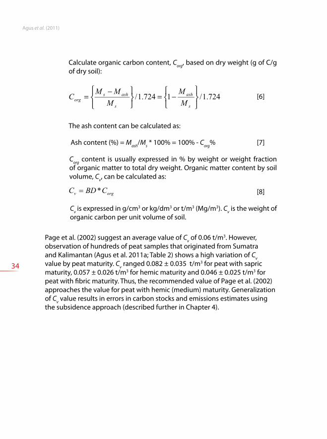
Calculate organic carbon content, Corg
, based on dry weight (g of C/g
of dry soil):
[6]
The ash content can be calculated as:
Ash content (%) = Mash
/Ms * 100% = 100% - C
org% [7]
Corg
content is usually expressed in % by weight or weight fraction
of organic matter to total dry weight. Organic matter content by soil
volume, Cv, can be calculated as:
[8]
Cv
is expressed in g/cm3 or kg/dm3 or t/m3 (Mg/m3). Cv is the weight of
organic carbon per unit volume of soil.
Page et al. (2002) suggest an average value of Cv of 0.06 t/m3. However,
observation of hundreds of peat samples that originated from Sumatra
and Kalimantan (Agus et al. 2011a; Table 2) shows a high variation of Cv
value by peat maturity. Cv ranged 0.082 ± 0.035 t/m3 for peat with sapric
maturity, 0.057 ± 0.026 t/m3 for hemic maturity and 0.046 ± 0.025 t/m3 for
peat with fibric maturity. Thus, the recommended value of Page et al. (2002)
approaches the value for peat with hemic (medium) maturity. Generalization
of Cv value results in errors in carbon stocks and emissions estimates using
the subsidence approach (described further in Chapter 4).
Practical guidelines Measuring carbon stock in peat soils
35
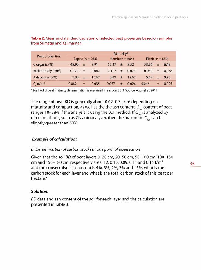
Table 2. Mean and standard deviation of selected peat properties based on samples
from Sumatra and Kalimantan
Peat propertiesMaturity*
Sapric (n = 263) Hemic (n = 904) Fibric (n = 659)
C organic (%) 48.90 ± 8.91 52.27 ± 8.52 53.56 ± 6.48
Bulk density (t/m3) 0.174 ± 0.082 0.117 ± 0.073 0.089 ± 0.058
Ash content (%) 9.98 ± 13.67 8.89 ± 12.67 5.69 ± 9.25
Cv (t/m3) 0.082 ± 0.035 0.057 ± 0.026 0.046 ± 0.025
* Method of peat maturity determination is explained in section 3.3.3. Source: Agus et al. 2011
The range of peat BD is generally about 0.02–0.3 t/m3 depending on
maturity and compaction, as well as the the ash content. Corg
content of peat
ranges 18–58% if the analysis is using the LOI method. If Corg
is analyzed by
direct methods, such as CN autoanalyzer, then the maximum Corg
can be
slightly greater than 60%.
Example of calculation:
(i) Determination of carbon stocks at one point of observation
Given that the soil BD of peat layers 0–20 cm, 20–50 cm, 50–100 cm, 100–150
cm and 150–180 cm, respectively are 0.12; 0.10, 0.09; 0.11 and 0.15 t/m3
and the consecutive ash content is 4%, 3%, 2%, 2% and 15%, what is the
carbon stock for each layer and what is the total carbon stock of this peat per
hectare?
Solution:
BD data and ash content of the soil for each layer and the calculation are
presented in Table 3.
Agus et al. (2011)
36
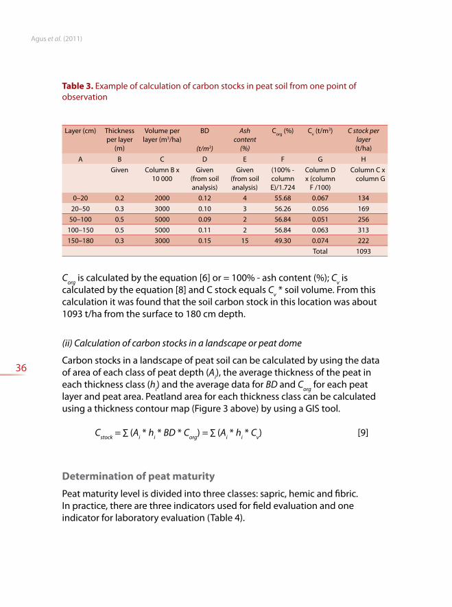
Table 3. Example of calculation of carbon stocks in peat soil from one point of
observation
Layer (cm) Thickness
per layer
(m)
Volume per
layer (m3/ha)
BD
(t/m3)
Ash
content
(%)
Corg
(%) Cv (t/m3) C stock per
layer
(t/ha)
A B C D E F G H
Given Column B x
10 000
Given
(from soil
analysis)
Given
(from soil
analysis)
(100% -
column
E)/1.724
Column D
x (column
F /100)
Column C x
column G
0–20 0.2 2000 0.12 4 55.68 0.067 134
20–50 0.3 3000 0.10 3 56.26 0.056 169
50–100 0.5 5000 0.09 2 56.84 0.051 256
100–150 0.5 5000 0.11 2 56.84 0.063 313
150–180 0.3 3000 0.15 15 49.30 0.074 222
Total 1093
Corg
is calculated by the equation [6] or = 100% - ash content (%); Cv is
calculated by the equation [8] and C stock equals Cv * soil volume. From this
calculation it was found that the soil carbon stock in this location was about
1093 t/ha from the surface to 180 cm depth.
(ii) Calculation of carbon stocks in a landscape or peat dome
Carbon stocks in a landscape of peat soil can be calculated by using the data
of area of each class of peat depth (Ai), the average thickness of the peat in
each thickness class (hi) and the average data for BD and C
org for each peat
layer and peat area. Peatland area for each thickness class can be calculated
using a thickness contour map (Figure 3 above) by using a GIS tool.
Cstock
= ∑ (Ai * h
i * BD * C
org) = ∑ (A
i * h
i * C
v) [9]
Determination of peat maturity
Peat maturity level is divided into three classes: sapric, hemic and fibric.
In practice, there are three indicators used for field evaluation and one
indicator for laboratory evaluation (Table 4).
Practical guidelines Measuring carbon stock in peat soils
37
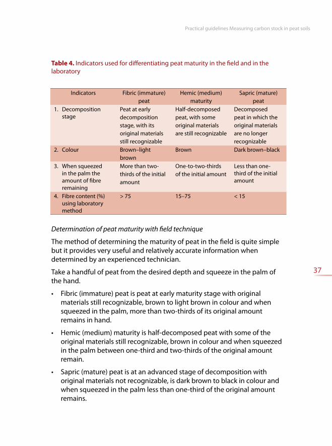
Table 4. Indicators used for differentiating peat maturity in the field and in the
laboratory
Indicators Fibric (immature)
peat
Hemic (medium)
maturity
Sapric (mature)
peat
1. Decomposition
stage
Peat at early
decomposition
stage, with its
original materials
still recognizable
Half-decomposed
peat, with some
original materials
are still recognizable
Decomposed
peat in which the
original materials
are no longer
recognizable
2. Colour Brown–light
brown
Brown Dark brown–black
3. When squeezed
in the palm the
amount of fibre
remaining
More than two-
thirds of the initial
amount
One-to-two-thirds
of the initial amount
Less than one-
third of the initial
amount
4. Fibre content (%)
using laboratory
method
> 75 15–75 < 15
Determination of peat maturity with field technique
The method of determining the maturity of peat in the field is quite simple
but it provides very useful and relatively accurate information when
determined by an experienced technician.
Take a handful of peat from the desired depth and squeeze in the palm of
the hand.
Fibric (immature) peat is peat at early maturity stage with original
materials still recognizable, brown to light brown in colour and when
squeezed in the palm, more than two-thirds of its original amount
remains in hand.
Hemic (medium) maturity is half-decomposed peat with some of the
original materials still recognizable, brown in colour and when squeezed
in the palm between one-third and two-thirds of the original amount
remain.
Sapric (mature) peat is at an advanced stage of decomposition with
original materials not recognizable, is dark brown to black in colour and
when squeezed in the palm less than one-third of the original amount
remains.
Agus et al. (2011)
38
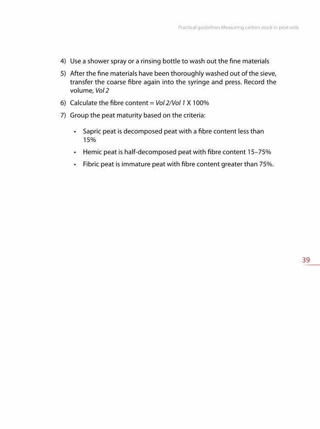
Determination of peat maturity in the laboratory
1) Fill a 10 ml or 25 ml syringe (Figure 17) with peat sample
2) Press the sample using the syringe pump and record the volume, Vol 1,
when the sample can no longer be compressed
3) Transfer the sample into a 150 μm or 0.0059 inch sieve
Figure 17. 10 ml syringe (left) and a sieve (right)
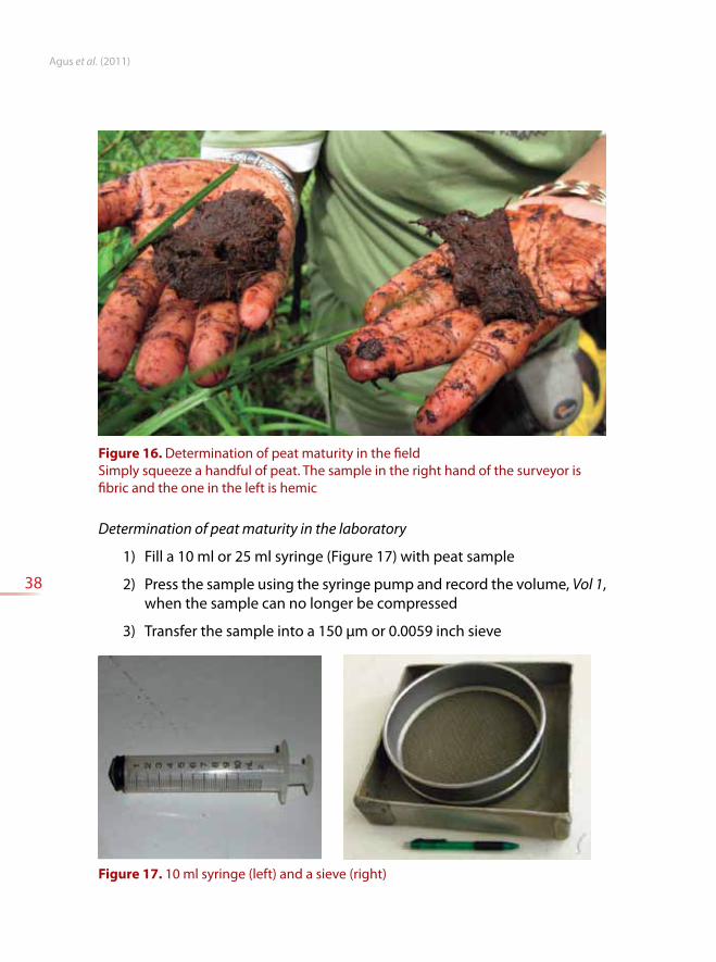
Figure 16. Determination of peat maturity in the field
Simply squeeze a handful of peat. The sample in the right hand of the surveyor is
fibric and the one in the left is hemic
Practical guidelines Measuring carbon stock in peat soils
39
4) Use a shower spray or a rinsing bottle to wash out the fine materials
5) After the fine materials have been thoroughly washed out of the sieve,
transfer the coarse fibre again into the syringe and press. Record the
volume, Vol 2
6) Calculate the fibre content = Vol 2/Vol 1 X 100%
7) Group the peat maturity based on the criteria:
Sapric peat is decomposed peat with a fibre content less than
15%
Hemic peat is half-decomposed peat with fibre content 15–75%
Fibric peat is immature peat with fibre content greater than 75%.

41
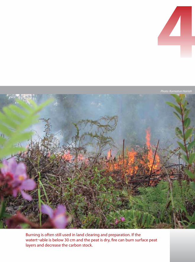
Burning is often still used in land clearing and preparation. If the
watert¬able is below 30 cm and the peat is dry, fire can burn surface peat
layers and decrease the carbon stock.
Photo: Kurniatun Hairiah

43
A reduction of carbon stock translates to carbon emissions and an increase in
carbon stock translates to carbon sequestration. Carbon emissions data are
normally expressed as CO2-e (CO
2 equivalent).
Peatland emits greenhouse gases in the forms of CO2, CH
4 (methane) and
N2O. Of the three gases, CO
2 is the most important because it forms the
highest amount emitted by peatland, especially converted peat forest
to agriculture or settlements. CH4 is measurable in peat forests that are
normally saturated or submerged. CO2 emissions dominate drained peat,
whereas CH4 emissions decrease significantly or even become undetectable
in drained peatland. N2O emissions occur from nitrogen-rich soils. Part of the
leached nitrate into the anaerobic layer is reduced into N2O. In general, CO
2
emissions from peat soil can be calculated based on the change in carbon
stocks within a given period of time.
Carbon storage in peatlands is the largest in (belowground) peat soil,
second, in the plant biomass and, third, in the necromass. Each component
of carbon stock may be increased or decreased depending on natural factors
and human intervention. Droughts result in a decreased watertable, which
could subsequently accelerate CO2 emissions from peat soils. Agricultural
land management practices on peatland, such as burning, construction of
drainage and fertilization affect CO2 emission levels. Peat fires can lower the
carbon stock in plant biomass and in the peat, which translates to increased
emissions from both sources. Fertilization can increase emissions owing to
increased microbial activity. On the other hand, reducing the depth of the
watertable in drained peatland through installation of canal blocking is likely
to reduce the amount of emissions.
Plant growth is a process of CO2 captured from the atmosphere through
photosynthesis and stored as carbon in plant tissue. The process of plant
growth, especially of tree crops, increases carbon stocks in a landscape.
Estimation of
greenhouse gas emissions
Agus et al. (2011)
44
Therefore, the amount of CO2 emissions at a certain time interval can be
estimated by the formula:
[10]
Ea
= Emissions owing to aboveground biomass decomposition
Ea = C
b x 3.67
Where Cb is the biomass (and necromass) carbon stocks that are subjected to
decomposition upon land-use conversion. The index 3.67 is the conversion
factor from C to CO2. According to the IPCC (2006), when land is cleared
it is assumed that all (100%) of plant biomass carbon is oxidized into CO2
through either burning or decomposition by microbes or a combination of
both. Supposing that a peat forest is cleared with aboveground carbon stock
in the plant biomass as high as 100 t/ha, then the amount of emissions from
this source are
Ea
= 100 t/ha C x 3.67 CO2/C = 367 t/ha CO
2 .
If the total forest area that was cleared was 6000 ha, then the emissions from
the plant biomass would be
Ea = 367 t/ha CO2 x 6,000 ha = 2,202,000 t CO
2.
The method for determining carbon stock in plant biomass is elaborated in
Hairiah et al. (2011a).
Ebb
= CO2 emissions owing to peat fire. When a layer of peat is completely
burned, then the organic matter will be oxidized, resulting in CO2 and
H2O and a number of other gases.
Ebb
= Volume of burnt peat (m3) x BD (t/m3) x Corg
(t/t) x 3.67 CO2/C
= Volume of burnt peat (m3) x Cv (t/m3) x 3,67 CO
2/C
The volume of burnt peat can be estimated by measuring the volume of the
peat basin formed after the fire, with the basin being the portion of initial
peat that is completely burned.
For example, if 6000 ha of peat with properties similar to the example in
Table 2 burnt evenly to a depth of 30 cm, then
( Ea
+ Ebb
+ Ebo— S
a)
tE =
Practical guidelines Measuring carbon stock in peat soils
45
The volume of burnt peat from the 0–20 cm layer = 0.2 m x 6000 ha x 10 000
m2/ha = 12 000 000 m3.
Ebb
(the amount of CO2 emissions from the 0–20 cm layer)
= Volume of burnt peat x Cv x 3,67
= 12 000 000 m3 x 0.067 t/m3 C x 3.67 CO2/C
= 2 950 680 t CO2
The volume of burnt peat from the 20–30 cm depth = 0.1 m x 6000 ha x 10
000 m2/ha = 6 000 000 m3.
Ebb
(the amount of CO2 emissions from 20–30 cm layer)
= 6 000 000 m3 * 0.056 t/m3 C x 3.67 CO2/C
= 1 233 120 t CO2
Total emission from the 0–30 cm layer
= 2 950 680 t CO2 + 1 233 120 t CO
2 = 4 183 800 t CO
2
Note: In reality the burning is never evenly distributed. It can enter into a few
metres of dry peat while some parts of the surface are only partially burnt.
Ebo
= Emissions from peat decomposition. There are various factors that
affect the rate of peat decomposition. The most important one is the depth
of the watertable, but under the same watertable emission rates can be
different depending on the maturity of the peat, fertilizer application and the
influence of plant root respiration. Plant root respiration must be discounted
from emission calculations because it is compensated by CO2 absorption
through photosynthesis.
Ebo
can be measured or estimated by several approaches, for example:
Measurement of greenhouse gas fluxes using CO2 Infra-Red Gas
Agus et al. (2011)
46
Analyzer (IRGA) or Gas Chromatography (GC)
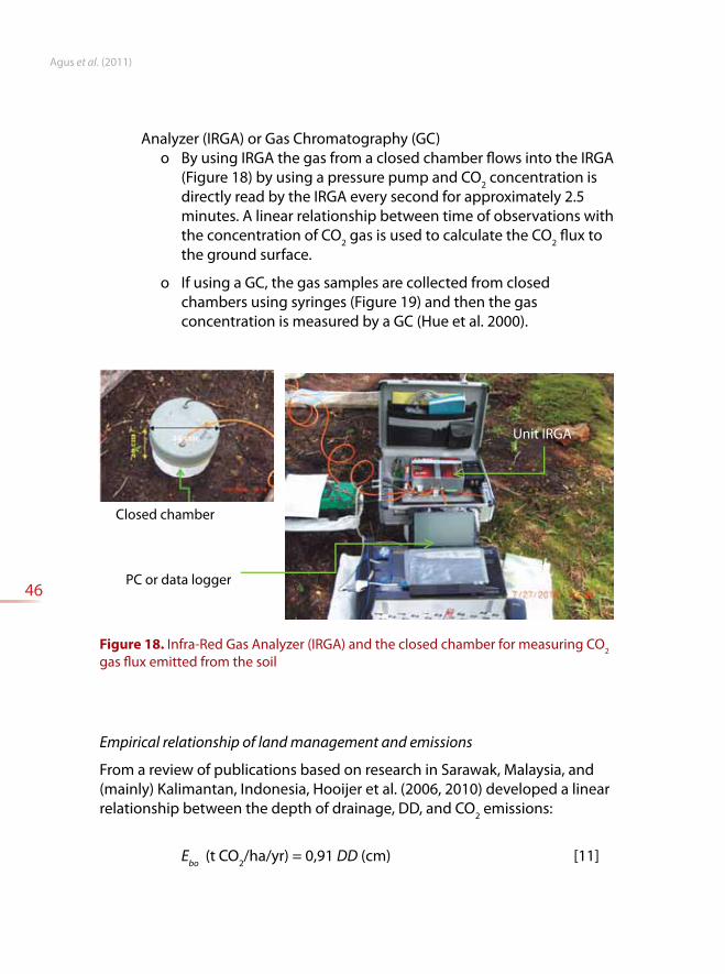
o By using IRGA the gas from a closed chamber flows into the IRGA
(Figure 18) by using a pressure pump and CO2 concentration is
directly read by the IRGA every second for approximately 2.5
minutes. A linear relationship between time of observations with
the concentration of CO2 gas is used to calculate the CO
2 flux to
the ground surface.
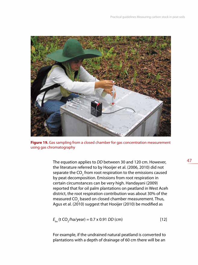
o If using a GC, the gas samples are collected from closed
chambers using syringes (Figure 19) and then the gas
concentration is measured by a GC (Hue et al. 2000).
Closed chamber
PC or data logger
Unit IRGA
Figure 18. Infra-Red Gas Analyzer (IRGA) and the closed chamber for measuring CO2
gas flux emitted from the soil
Empirical relationship of land management and emissions
From a review of publications based on research in Sarawak, Malaysia, and
(mainly) Kalimantan, Indonesia, Hooijer et al. (2006, 2010) developed a linear
relationship between the depth of drainage, DD, and CO2 emissions:
Ebo
(t CO2/ha/yr) = 0,91 DD (cm) [11]
Practical guidelines Measuring carbon stock in peat soils
47The equation applies to DD between 30 and 120 cm. However,
the literature referred to by Hooijer et al. (2006, 2010) did not
separate the CO2 from root respiration to the emissions caused
by peat decomposition. Emissions from root respiration in
certain circumstances can be very high. Handayani (2009)
reported that for oil palm plantations on peatland in West Aceh
district, the root respiration contribution was about 30% of the
measured CO2 based on closed chamber measurement. Thus,
Agus et al. (2010) suggest that Hooijer (2010) be modified as
Ebo
(t CO2/ha/year) = 0.7 x 0.91 DD (cm) [12]
For example, if the undrained natural peatland is converted to
plantations with a depth of drainage of 60 cm there will be an
Figure 19. Gas sampling from a closed chamber for gas concentration measurement
using gas chromatography
Agus et al. (2011)
48
increase of CO2 emissions:
Ebo
= 0.7 x 0.91 t CO2/ ha / yr / cm x 60 cm = 38.22 t CO2/ ha / yr.
If the area of the converted land is 6000 ha for an oil palm
plantation cycle of 25 years then
Ebo
= 0.7 x 0.91 t CO2 /ha/yr/cm x 60 cm x 6000 ha x 25 yr
= 5 733 000 t CO2 = 5.7 Mt CO
2
Estimate based on peat subsidence
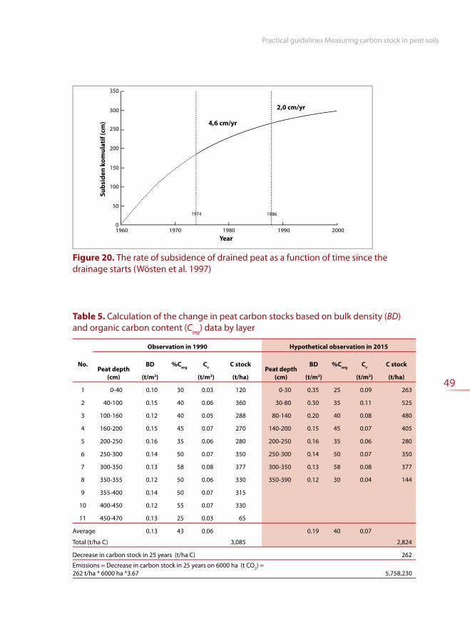
According to Wösten et al. (1997), subsidence takes place very rapidly
in the first few years after the drainage is initiated and achieves stability
at the rate of about 2 cm/yr (Figure 20). They explained further that,
assuming that there is no fire, then the decomposition accounts for 60% of
subsidence, while compaction (consolidation) accounts for 40%. In contrast,
Couwenberg (2010) estimated that the decomposition of peat accounted for
approximately 40% of subsidence. That is, if subsidence occurs as thick as 10
cm, 4 cm is attributable to peat decomposition and 6 cm due to compaction
and consolidation.
Based on Couwenberg (2010), supposing that within 25 years a landscape
of peat undergoes 50 cm subsidence, then 40% x 50 cm = 20 cm of the
subsidence is caused by peat decomposition. If the volume-based carbon
content, Cv = 0.06 t /m3, then from the 6000 ha of peatland, emissions that
occur during 25 years would be
Ebo
= 0.20 m x 0.06 t/m3 C x 3.67 t CO2/t C x 6000 ha x 10 000 m2/ha
= 2 642 000 t CO2 = 2.6 Mt CO2
Estimation based on changes in carbon stocks in peat
This estimate is based on the difference in carbon stocks in peat at time t1,
for example, when peatland is still covered by natural forest and at time t2,
after a few years of drainage. Carbon content and BD measurements were
done by layers from the surface to the peat bottom at time t1 and t
2. Sample
calculations in Table 5 provide the data of BD and Corg
, at t1 and t
2 in 1990 and
2015, respectively. This approach provides an estimate of emissions as much
as 5.8 million t CO2 over 25 years (Table 5).
Practical guidelines Measuring carbon stock in peat soils
49
Figure 20. The rate of subsidence of drained peat as a function of time since the
drainage starts (Wösten et al. 1997)
350
300
250
200
150
100
1960 1970 1980
Year
4,6 cm/yr
Su
bsi
de
n k
om
ula
tif
(cm
)2,0 cm/yr
1990 2000
50
0
19861974
Table 5. Calculation of the change in peat carbon stocks based on bulk density (BD)
and organic carbon content (Corg
) data by layer
Observation in 1990 Hypothetical observation in 2015
No.Peat depth
(cm)
BD %Corg
Cv
C stock Peat depth
(cm)
BD %Corg
Cv
C stock
(t/m3) (t/m3) (t/ha) (t/m3) (t/m3) (t/ha)
1 0-40 0.10 30 0.03 120 0-30 0.35 25 0.09 263
2 40-100 0.15 40 0.06 360 30-80 0.30 35 0.11 525
3 100-160 0.12 40 0.05 288 80-140 0.20 40 0.08 480
4 160-200 0.15 45 0.07 270 140-200 0.15 45 0.07 405
5 200-250 0.16 35 0.06 280 200-250 0.16 35 0.06 280
6 250-300 0.14 50 0.07 350 250-300 0.14 50 0.07 350
7 300-350 0.13 58 0.08 377 300-350 0.13 58 0.08 377
8 350-355 0.12 50 0.06 330 350-390 0.12 30 0.04 144
9 355-400 0.14 50 0.07 315
10 400-450 0.12 55 0.07 330
11 450-470 0.13 25 0.03 65
Average 0.13 43 0.06 0.19 40 0.07
Total (t/ha C) 3,085 2,824
Decrease in carbon stock in 25 years (t/ha C) 262
Emissions = Decrease in carbon stock in 25 years on 6000 ha (t CO2) =
262 t/ha * 6000 ha *3.67 5,758,230
Agus et al. (2011)
50
Sa= Sequestration or CO
2 uptake by plants = the time-averaged carbon
stock in the biomass and necromass of the succeeding plants (t/
ha) x 3.67. For example, if the time-averaged carbon stock from one
economic time cycle of 25 years of oil palm = 40 t/ha C, then for 6000
ha of land, its contribution in reducing CO2 in the atmosphere = 40 t/ha
C ha x 6000 x 3.67 t CO2/C = 880 800 t CO
2.
Δt = The time period for the calculation, which depends on the purpose of
the analysis. It could be 1 minute or 1 hour in terms of gas flux, 1 year
or several years for plant growth, as long as all factors in the calculation
(Equation 10) use the same time period. For carbon trading, a long
time scale of, for example, 10–20 years, is normally used.
By using the above calculation and Table 5 for Ebo
, and combining them to
Equation [10], then
E = (2,202,000 + 4,183,800 + 5,758,230 – 880,800) t CO2/25 years
= 11,262,430 t CO2/25 yr/6,000 ha, and this is equivalent with
= 75 t CO2/ha/year
From this calculation it can be interpreted that about 11 million tonne (Mt)
of CO2 would be emitted within 25 years from the 6000 ha peat forest that
was converted to plantation. From the perspective of REDD, it can be stated
that about 11 Mt CO2/25 yr/6000 ha can be reduced by maintaining the peat
forest as is (by avoiding deforestation).
( Ea
+ Ebb
+ Ebo— S
a)
tE =

51
Discussion
In REDD or any similar emission reduction scheme, the service providers of
carbon conservation are entitled for payment from the carbon service buyers
based on a formal agreement. The amount of payment may be based on
the internationally published price of carbon or on the ‘opportunity cost’ of
forgone benefits from alternative business on the land.
What should a country, a province or district consider prior to engagement
in carbon trading? They should first understand and convince themselves of
several issues.
Whether the price of carbon offered by the buyers can cover the
opportunity and transaction costs. In other words, whether the seller of
the service is willing to accept the amount of payment.
Whether government at national and sub-national levels, as well as the
local community, can obey the long-term commitment (in this example,
25 years, but it may be 10, 20 or longer than 25) not to cut or drain the
peat forest.
Whether avoiding deforestation on the land under contract can avoid
‘leakage’, that is, an increase in deforestation and land conversion in
surrounding areas.
If the answer to each of the three question is ‘yes’, it indicates that both the
carbon buyers and sellers are ready for carbon trading.
Apart from carbon trading, a decrease in carbon stock is associated with peat
subsidence. Peat subsidence is highly related to sustainability of farming
on peatland. Before using peatlands for agriculture we need to consider the
sustainability and environmental aspects (Agus and Subiksa 2008). For those
lands that have been used for agriculture, it is imperative to implement
the best management techniques for sustaining the business. Given the
relatively low productivity of peatlands and their important role as a buffer
of environmental quality, then the future development of peatland for
agriculture should be kept to a minimum.

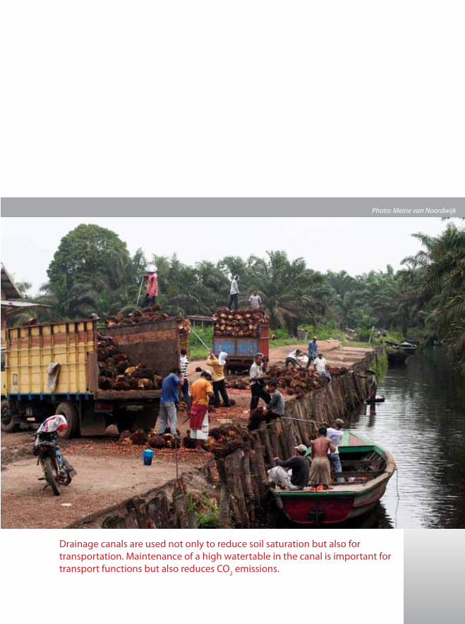
Drainage canals are used not only to reduce soil saturation but also for
transportation. Maintenance of a high watertable in the canal is important for
transport functions but also reduces CO2 emissions.
Photo: Meine van Noordwijk

55
Aguilar FJ, Agüera F, Aguilar MA, Carvajal F. 2005. Effects of terrain
morphology, sampling density and interpolation methods on grid DEM
accuracy. Photogrammetric Engineering and Remote Sensing 71(7):805–
816.
Agus F, Wahyunto, Mulyani A, Dariah A, Maswar, Susanti E. 2011. Variasi stock
karbon dan emisi CO2 di lahan gambut. Laporan Tengah Tahun KP3I.
Variations in carbon stocks and emissions of CO2 in peatlands. Mid-year
report KP3I. Bogor, Indonesia: Balai Besar Litbang Sumberdaya Lahan
Pertanian. In press.
Agus F, Subiksa IGM. 2008. Lahan gambut: potensi untuk pertanian dan aspek
lingkungan. Peatlands: potential for agriculture and the environmental
aspect. Bogor, Indonesia: Balai Penelitian Tanah; World Agroforestry
Centre (ICRAF) Southeast Asia Regional Program.
Agus F, Handayani E, Van Noordwijk M, Idris K, Sabiham S. 2010. Root
respiration interference with peat CO2 emission measurement. In:
Proceedings Nineteenth World Congress of Soil Science, 1–6 August 2010,
Brisbane, Australia. DVD. Brisbane, Australia: International Union of Soil
Sciences. p. 50–53.
Boer R, Sulistyowati, Las I, Zed F, Masripatin N, Kartakusuma DA, Hilman D,
Mulyanto HS. 2010. Indonesia’s second national communication under
the United Nations Framework Convention on Climate Change. Jakarta:
Ministry of the Environment.
Couwenberg J, Dommain R, Joosten H. 2010. Greenhouse gas fluxes from
tropical peatlands in Southeast Asia. Global Change Biology 16:1715–
1732.
Dixon RK, Brown S, Houghton RA, Solomon AM, Trexler MC, Wisniewski
J. 1994. Carbon pools and flux of global forest ecosystems. Science
263:185–191.
References
Agus et al. (2011)
56
Hairiah K, Rahayu S. 2007. Pengukuran ‘cadangan karbon’ di berbagai macam
penggunaan lahan. Measurement of carbon stocks in a wide range
of land uses. Bogor, Indonesia: World Agroforestry Centre (ICRAF)
Southeast Asia Regional Program; Malang, Indonesia: Universitas
Brawijaya.
Hairiah K, Ekadinata A, Sari RR, Rahayu S. 2011a. Pengukuran cadangan
karbon dari tingkat lahan ke bentang lahan. Edisi 2. Measurement of
carbon stocks from plot to landscape level. Second Edition. Bogor,
Indonesia: World Agroforestry Centre (ICRAF) Southeast Asia Regional
Program; Malang, Indonesia: Universitas Brawijaya.
Hairiah K, Dewi S, Agus F, Velarde SJ, Ekadinata A, Rahayu S, van Noordwijk
M. 2011b. Measuring carbon stocks across land-use systems: a manual.
Bogor, Indonesia: World Agroforestry Centre (ICRAF) Southeast Asia
Regional Program.
Handayani E. 2009. Emisi karbon dioksida (CO2) dan metan (CH
4) pada
perkebunan kelapa sawit di lahan gambut yang memiliki keragaman
dalam ketebalan gambut dan umur tanaman. Emissions of carbon
dioxide (CO2) and methane (CH
4) in oil palm plantations on peatlands
have diversity in the thickness of peat and plant age. PhD Thesis.
Bogor, Indonesia: Institut Pertanian Bogor.
Hooijer A, Page S, Canadell JG, Silvius M, Kwadijk J, Wösten H, Jauhiainen
J. 2010. Current and future CO2 emissions from drained peatlands in
Southeast Asia. Biogeosciences 7:1505–1514.
Hooijer A, Silvius M, Wösten H, Page S. 2006. PEAT-CO2: assessment of CO
2
emissions from drained peatlands in SE Asia. Delft Hydraulics report
Q3943 (2006). Delft, The Netherlands: WL/Delft Hydraulics.
Hue AX, Chen GX, Wang ZP, Van Cleemput O, Patrick Jr WH. 2000. Methane
and nitrous oxide emissions from a rice field in relation to soil redox
and microbiological processes. Soil Science Society of America Journal
64:2180–2186.
[IPCC] Intergovernmental Panel on Climate Change. 2006. IPCC guidelines
for national greenhouse gas inventories. Eggleston HS, Buendia L,
Miwa K, Ngara T, Tanabe K, eds. Prepared by the National Greenhouse
Gas Inventories Programme. Hayama, Japan: Institute for Global
Environmental Studies.
Practical guidelines Measuring carbon stock in peat soils
57
Jaenicke J, Wösten H, Budiman AA, Siegert F. 2010. Planning hydrological
restoration of peatlands in Indonesia to mitigate carbon dioxide
emissions. Mitigation and Adaptation Strategies for Global Change
15(3):223–239.
Maswar. 2011. Kajian cadangan karbon pada lahan gambut tropika yang
didrainase untuk tanaman tahunan. Study of carbon stocks in tropical
peatland drained for annual crops. Bogor, Indonesia: Sekolah
Pascasarjana, Institut Pertanian Bogor.
Murdiyarso D, Rosalina U, Hairiah K, Muslihat L, Suryadiputra INN, Jaya A.
2004. Petunjuk lapangan: Pendugaan Cadangan Karbon pada Lahan
Gambut. Field tips: estimation of carbon in peatland reserves. Bogor,
Indonesia: Wetlands International Indonesia Program; Ottawa: Wildlife
Habitat Canada.
Noor M. 2001. Pertanian lahan gambut: potensi dan kendala. Peatland:
potential and constraints. Jakarta: Penerbit Kanisius.
Page SE, Siegert F, Rieley JO, Boehm HV, Jaya A, Limin S. 2002. The amount
of carbon released from peat and forest fires in Indonesia during 1997.
Nature 420:61–65.
Ritung, S., Wahyunto, Nugroho, K., Sukarman, Hikmatullah, Suparto,
Tafakresnanto, C. 2011. Peta Lahan Gambut Indonesia Skala 1:250.000
(Indonesian peatland map at the scale 1:250,000). Indonesian Center
for Agricultural Land Resources Research and Development, Bogor,
Indonesia.
Shofiyati R, Las I, Agus F. 2010. Indonesian soil database and predicted stock
of soil carbon. In: Chen ZS, Agus F, eds. Proceedings of international
workshop on evaluation and sustainable management of soil carbon
sequestration in Asian countries. 28–29 September 2010. Bogor,
Indonesia. Bogor, Indonesia: Indonesian Soil Research Institute; Taipei:
Food and Fertilizer Technology Center for the Asian and Pacific Region;
Tsukuba, Japan: National Institute for Agro-Environmental Sciences. p.
73–83.
Suganda H, Rachman A, Sutono. 2007. Petunjuk pengambilan contoh tanah.
Soil sampling instructions. In: Kurnia U, Agus F, Adimihardja A, Dariah
A, eds. Sifat fisik tanah dan metode analisisnya. Soil physical properties
and analytical methods. Bogor, Indonesia: Balai Penelitian Tanah. p.
3–24.
Agus et al. (2011)
58
Van de Meene J. 1984. Geological aspects of peat formation in the
Indonesian-Malaysian lowlands. Bulletin Geological Research and
Development Centre 9:20–31.
Wahyunto, Ritung S, Suparto, Subagjo H. 2004. Map of peatland distribution
area and carbon content in Kalimantan. Bogor, Indonesia: Wetlands
International Indonesia Program; Ottawa: Wildlife Habitat Canada.
Wahyunto, Ritung S, Suparto, Subagjo H. 2005. Peatland distribution and
carbon content in Sumatra and Kalimantan. Bogor, Indonesia: Wetlands
International Indonesia Program; Ottawa: Wildlife Habitat Canada.
Wahyunto, Suparto, Heryanto B, Bekti H. 2006. Sebaran lahan gambut,
luas dan cadangan karbon bawah permukaan di Papua. Peatland
distribution, extent and belowground carbon stocks in Papua. Bogor,
Indonesia: Wetlands International Indonesia Program.
Walkley A, Black IA. 1934. An examination of Degtjareff method for
determining soil organic matter and a proposed modification of the
chromic acid titration method. Soil Science 37:29–37.
Wösten JHM, Ismail AB, van Wijk ALM. 1997. Peat subsidence and its practical
implications: a case study in Malaysia. Geoderma 78:25–36.
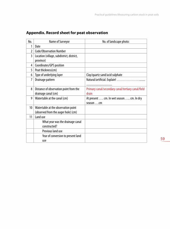
Practical guidelines Measuring carbon stock in peat soils
59
Appendix. Record sheet for peat observation
No. Name of Surveyor No. of landscape photo:
1 Date
2 Code/Observation Number
3 Location (village, subdistrict, district,
province)
4 Coordinates/GPS position
5 Peat thickness(cm)
6 Type of underlying layer Clay/quartz sand/acid sulphate
7 Drainage pattern Natural/artificial. Explain! ………………........
...................................
8 Distance of observation point from the
drainage canal (cm)
Primary canal/secondary canal/tertiary canal/field
drain
9 Watertable at the canal (cm) At present …. cm. In wet season….. cm. In dry
season …cm
10 Watertable at the observation point
(observed from the auger hole) (cm)
11 Land use
What year was the drainage canal
constructed?
Previous land use
Year of conversion to present land
use

Agus et al. (2011)
60
12 Sample code and numbering for each
layer (must appear on this form and in the
sample plastic bags)
No. Code and date Depth (cm) Maturity Remarks (e.g. in case of the presence of clay or
charcoal layer, record at what depth and how thick)
1
2
3
4
5
6
7
8
9
10
11
12
13
14
15
16
17
18
19
20
Indonesian Centre for Agricultural Land
Resources Research and Development