Measuring Bedload Sediment Transport with an … · sdz ð1 Þ where z s = water surface level; z b = immobile bed level; u s = sediment velocity; and c s = sediment concentration

Measuring Bedload Sediment Transport with anAcoustic Doppler Velocity Profiler

Koen Blanckaert, M.ASCE1; Joris Heyman2; and Colin D. Rennie, M.ASCE3

Abstract: Acoustic Doppler velocity profilers (ADVP) measure the velocity simultaneously in a linear array of bins. They have beensuccessfully used in the past to measure three-dimensional turbulent flow and the dynamics of suspended sediment. The capability of ADVPsystems to measure bedload sediment flux remains uncertain. The main outstanding question relates to the physical meaning of the velocitymeasured in the region where bedload sediment transport occurs. The main hypothesis of the paper, that the ADVP measures the velocity ofthe moving bedload particles, is validated in laboratory experiments that range from weak to intense bedload transport. First, a detailedanalysis of the raw return signals recorded by the ADVP reveals a clear footprint of the bedload sediment particles, demonstrating thatthese are the main scattering sources. Second, time-averaged and temporal fluctuations of bedload transport derived from high-speedvideography are in good agreement with ADVP estimates. Third, ADVP based estimates of bedload velocity and thickness of the bedloadlayer comply with semi-theoretical expressions based on previous results. An ADVP configuration optimized for bedload measurementsis found to perform only marginally better than the standard configuration for flow measurements, indicating that the standard ADVPconfiguration can be used for sediment flux investigations. Data treatment procedures are developed that identify the immobile-bed surface,the layers of rolling/sliding and saltating bedload particles, and the thickness of the bedload layer. Combining ADVP measurements ofthe bedload velocity with measurements of particle concentration provided by existing technology would provide the sediment flux.DOI: 10.1061/(ASCE)HY.1943-7900.0001293. © 2017 American Society of Civil Engineers.

Author keywords: Bedload transport; Acoustics; Three-dimensional acoustic Doppler velocity profiler (3D-ADVP); Digital videography;Particle velocimetry; Optical flow.

Introduction

Problem Definition

Knowledge of the quantity of sediment transported in rivers isof paramount importance in, for example, the understanding andprediction of morphological evolution, hazard mapping and miti-gation, or the design of hydraulic structures like bridge piers orbank protections. However, measurement of the sediment flux isnotoriously difficult, especially during high flow conditions whenmost sediment transport occurs.

The sediment flux per unit width can be expressed as

qs ¼Z

zs

zb

uscsdz ð1Þ

where zs = water surface level; zb = immobile bed level; us =sediment velocity; and cs = sediment concentration. The total sedi-ment flux is the most relevant variable with respect to the river mor-phology. However, it is often separated in fluxes of suspended load

sediment transport and bedload sediment transport. Suspended loadrefers to sediment particles that are transported in the body of theflow, being suspended by turbulent eddies. Because of their smallsize (and therefore their small Stokes number), suspended particlestend to follow the flow streamlines; thus, their velocities are close tothe velocities of the turbulent flow. In contrast, bedload involveslarger sediment particles that slide, roll, and saltate on the bed, thusremaining in close contact with it. The friction and the frequentcollisions of bedload particles with the granular bed reduce theirvelocity considerably. Because of drag forces, fluid velocities mayalso be reduced inside the bedload layer.

Accurate measurement of bedload transport has long been agoal of river and coastal scientists and engineers (e.g., Mulhoffer1933). Conventional measurements with physical samplers are lim-ited in spatial and temporal resolution, are cost prohibitive as aresult of substantial manual labor, and can be difficult and/or dan-gerous to conduct during high channel-forming flows when mostbed material transport occurs. Videography techniques have beendeveloped for laboratory settings and well-controlled flows (Drakeet al. 1988; Radice et al. 2006; Roseberry et al. 2012; Heyman2014), but are hindered when intense suspended sediment transportoccurs as a result of the turbidity of the water. They are particularlydifficult to use in the field, especially under high-flow conditionswhen intense sediment transport occurs. Consequently, little isknown about the temporal and particularly the spatial distributionof fluvial bedload, other than the recognition that the spatiotempo-ral distribution of bed material transport determines the channelform (Ferguson et al. 1992; Church 2006; Seizilles et al. 2014;Williams et al. 2015).

Acoustic Doppler current profiler (ADCP) backscatter intensityand/or attenuation have been used to estimate suspended sedimentconcentration and grain size (e.g., Guerrero et al. 2011, 2013, 2016;

1Senior Scientist, Ecological Engineering Laboratory, ENAC, EcolePolytechnique Fédérale Lausanne, 1015 Lausanne, Switzerland; Distin-guished Visiting Researcher, Univ. of Ottawa, Ottawa, ON, CanadaK1N 6N5 (corresponding author). E-mail: [email protected]

2Postdoctoral Researcher, UMR CNRS 6251, Institut de Physique deRennes, 35042 Rennes, France. E-mail: [email protected]

3Professor, Univ. of Ottawa, Ottawa, ON, Canada K1N 6N5. E-mail:[email protected]

Note. This manuscript was submitted on May 12, 2016; approved onOctober 17, 2016; published online on February 16, 2017. Discussionperiod open until July 16, 2017; separate discussions must be submittedfor individual papers. This paper is part of the Journal of HydraulicEngineering, © ASCE, ISSN 0733-9429.

© ASCE 04017008-1 J. Hydraul. Eng.

J. Hydraul. Eng., -1--1

Dow

nloa

ded

from

asc

elib

rary

.org

by

Hon

g K

ong

Uni

vers

ity o

f Sc

i and

Tec

h (H

KU

ST)

on 0

2/23

/17.

Cop

yrig

ht A

SCE

. For

per

sona

l use

onl

y; a

ll ri

ghts

res

erve

d.

https://doi.org/10.1061/(ASCE)HY.1943-7900.0001293

mailto:[email protected]



Moore et al. 2013; Latosinski et al. 2014). Rennie et al. (2002),Rennie and Church (2010), and Williams et al. (2015) used thebias in ADCP bottom tracking (Doppler sonar) as a measure ofapparent bedload velocity. Because of the diverging beams ofADCP, this technique may provide only an indication of bedloadparticle velocities averaged over the bed surface insonified by thefour beams. This technique also does not provide the thickness andconcentration of the active bedload layer, which are required to de-termine the bed load flux (Rennie and Villard 2004; Gaueman andJacobson 2006).

ADVP, which uses beams that converge in one single area ofmeasuring bins, has commonly been used to investigate turbulentflows (Fig. 1). Its application range has recently been extended tothe investigation of the dynamics of transported sediment, primarilytransport in suspension [Crawford and Hay 1993; Thorne andHardcastle 1997; Shen and Lemmin 1999; Cellino and Graf 2000;T. P. Stanton, “Bistatic Doppler velocity and sediment profiler de-vice for measuring sediment concentration, estimates profile ofmass flux from the product of mass concentration and three com-ponent velocity vector, US Sec of Navy,” Patent No. US6262942-B1 (2001); Smyth et al. 2002; Thorne and Hanes 2002; Hurtheret al. 2011; Thorne et al. 2011; Thorne and Hurther 2014]. Thepresent paper focuses on its use for the measurement of bedloadsediment transport.

ADVP: Working Principle and State of the Art

The working principle of ADVP has been detailed previously[Lemmin and Rolland 1997; Hurther and Lemmin 1998; Thorneet al. 1998; Shen and Lemmin 1999; Stanton and Thornton 1999;T. P. Stanton, “Bistatic Doppler velocity and sediment profiler de-vice for measuring sediment concentration, estimates profile ofmass flux from the product of mass concentration and three com-ponent velocity vector, US Sec of Navy,” Patent No. US6262942-B1 (2001); Zedel and Hay 2002]. The main features of the ADVP’sworking principle that are required for making the present paperself-contained are summarized as follows. An ADVP consists ofa central beam emit transducer surrounded by multiple fan-beamreceive transducers [Fig. 1(a)]. The instrument is typically set up

on a fixed mount pointing down toward the bed, and measuressimultaneously velocities in the water column situated between theemitter and the bed. This water column is divided into individualbins of O(mm). The profiling range, i.e. the height of the measuredwater column, is typically O(m). The emit transducer sends a seriesof short acoustic pulses vertically down toward the bed with auser-defined pulse repetition frequency (PRF) and pulse length.These pulses are reflected by scattering sources in the water, anda portion of this scattered sound energy is directed toward the re-ceive transducers. Turbulence-induced air bubble microstructuresin sediment-free clear water (Hurther 2001) or sediment particlesin sediment-laden flows (Hurther et al. 2011) can be scatteringsources of this instrument. For each bin in the water column, thebackscattered signal recorded by each of the receivers can bewritten as

aðtÞ ¼ A cos½2πðf0 þ fDÞt� ð2Þ

where A = amplitude of the recorded signal; and fD = Doppler fre-quency shift. The latter is proportional to the velocity componentdirected along the bisector of the backscatter angle [Fig. 1(b)] asfollows:

fD ¼ 2f0c

~V:~eB ð3Þ

where c = speed of sound in water; ~V = vectorial velocity of thescattering source; and ~eB = unit vector along the bisector of thebackscatter angle for the considered bin. To compute fD, the re-corded signal aðtÞ is typically demodulated into in-phase and quad-rature components, represented by IðtÞ and QðtÞ, and measured involts. The Doppler frequency fDðtÞ corresponds to the frequencyof these oscillating IðtÞ and QðtÞ signals. The demodulation intoin-phase and quadrature parts is necessary to determine the sign offD. The quasi-instantaneous Doppler frequency is typically com-puted with the pulse-pair algorithm using number-of-pulse-pairs(NPP) samples of IðtÞ and QðtÞ as follows (Miller and Rochwarger1972; Lhermitte and Serafin 1984; Zedel et al. 1996; Zedel andHay 2002):

Water-filled box

0

0.05

0.1

0.15

0.2

0.25

0.3

0.35

-0.15 -0.1 -0.05 0 0.05 0.1 0.15

x [m]

z [m

]

0.05

0.1

0.15

0.2

0.25

0.3

0.35

x [m]

z [m

]

dh

dv

Pulse emitted at PRF with frequency f0

Flow

Sediment

Water surface

~0.01 m

-0.15 -0.1 -0.05 0 0.05 0.1 0.150

0.05

0.1

0.15

0.2

Flow

x [m]

z [m

]

Sediment~0.01 m

605550454035302520

AD

VP

Bin

num

ber

dh

dv

Pulse emitted at PRF with frequency f0

Water surface

V

V.eB

back

scat

ter a

ngle

at il

lust

rate

d bi

n

(a) (b)

Fig. 1. (Color) Acoustic Doppler velocity profiler and digital video camera; the red arcs define the ellipses of equal acoustic path travel time betweenthe send and receive transducers for the bed bin (bottom arc) and the first bin above the bed (top arc): (a) standard ADVP configuration optimized forflow measurements in the body of the water column; (b) ADVP configuration optimized for bedload measurements; (c) simultaneous deployment ofthe ADVP optimized for bedload measurements and a digital video camera focused on the same near-bed sample volume



Dow

nloa

ded

from

asc

elib

rary

.org

by

Hon

g K

ong

Uni

vers

ity o

f Sc

i and

Tec

h (H

KU

ST)

on 0

2/23

/17.

Cop

yrig

ht A

SCE

. For

per

sona

l use

onl

y; a

ll ri

ghts

res

erve

d.

f̂D ¼ PRF2π

tan−1�PNPP−1

s¼1 QsIsþ1 þ IsQsþ1PNPP−1s¼1 IsIsþ1 þQsQsþ1

�ð4Þ

where ^ = average over NPP time samples; and s = time index. TheNPP has to be chosen high enough to assure second-order statio-narity, but low enough so that NPP/PRF remains small comparedwith the characteristic timescale of the investigated turbulent flow.Use of at least three receive transducers allows for measurement ofall three velocity components. Beam velocities are converted toCartesian coordinates using a beam transformation matrix specificfor the beam geometry.

Acoustic concentration and velocity profilers, which integratean ADVP and an acoustic backscatter system (ABS), have beensuccessfully used to investigate suspended sediment fluxes, definedas the product of sediment velocity and sediment concentration[Eq. (1)]. The ADVP measures the velocity of the suspended sedi-ment, which is assumed to be equal to the flow velocity. The ABSprovides the particle concentration in bins throughout a profile, andis obtained based on the range-gated acoustic backscatter intensityand/or attenuation (e.g., Crawford and Hay 1993; Thorne andHardcastle 1997; Shen and Lemmin 1999; Thorne and Hanes 2002;Hurther et al. 2011; Thorne et al. 2011; Thorne and Hurther 2014;Wilson and Hay 2015a, b). These measurements have permitteddirect examination of suspended sediment transport as a functionof flow forcing. For example, Smyth et al. (2002) used an ADCPsystem to document periodic sediment suspension associated withturbulent vortex shedding from ripples in a wave bottom boun-dary layer.

A broadband multifrequency ADCP, called MFDop, capable of0.0009 m vertical resolution at 85 Hz, was recently developed byHay et al. (2012a, b, c); it allows for estimation of both particleconcentration and grain size (Crawford and Hay 1993; Thorneand Hardcastle 1997; Wilson and Hay 2015a, b). For this system,velocities measured in bins within 0.005 m of a fixed bed weredeemed to be negatively biased, based on nonconformity with theprofiles of both log-law velocity and phase shift expected in a wavebottom boundary layer. This bias occurred largely because equaltravel time paths between send and receive transducers includedbottom echo for bins close to the bed [Figs. 1(a and b)]. However,the system was able to measure the bed velocity (of an oscillatorycart) based on Doppler processing of the signal at the observedbottom range.

Hurther et al. (2011) recently developed acoustic concentrationand velocity profiler (ACVP), which combines an ADVP with ad-vanced noise reduction for turbulence statistics (Blanckaert andLemmin 2006, Hurther and Lemmin 2008) with the ABS systemdeveloped by Thorne and Hanes (2002). The ACVP measuresco-located, simultaneous profiles of both two-component velocityand sediment concentration referenced to the exact position at thebed. Measurements are performed with high temporal (25 Hz) andspatial (bin size of 0.003 m) resolution. Sediment concentrationprofiles are determined by applying the dual-frequency inversionmethod (Bricault 2006; Hurther et al. 2011), which offers theunique advantage of being unaffected by the nonlinear sedimentattenuation across highly concentrated flow regions, and thus al-lows for the measurement of high sediment concentrations nearthe bed where the bedload transport occurs. The acoustic theoryunderpinning the dual-frequency inversion method is based on thecondition of negligible multiple scattering (Hurther et al. 2011).Although this condition is probably violated in the bedload layer,Naqshband et al. (2014b; Fig. 12) successfully applied the methodto estimate the sediment concentration all through the bedload layeronto the immobile bed, where a bulk concentration of ρsð1 − εÞ ¼1,590 kgm−3 was correctly measured (ε is the porosity of the

immobile sediment bed). These results indicate that the theoreticalcondition of negligible multiple scattering can be relaxed, and thatthe dual-frequency inversion method is also able to measure thehigh sediment concentrations in the bedload layer. The ACVP hasbeen used to measure velocity, concentration profiles, and sedimentfluxes over ripples under shoaling waves (Hurther and Thorne2011) and over migrating equilibrium sand dunes (Naqshband et al.2014a, b). An acoustic interface detection method was used to iden-tify the immobile bed and the suspended load layer and a layer inbetween with higher sediment concentrations (Hurther and Thorne2011; Hurther et al. 2011). Hurther and Thorne (2011) acknowl-edged uncertainty in the identification of the near-bed layer withhigh sediment concentration, but found that the estimated sedimentflux matched estimates based on ripple migration. They termed thislayer the “near-bed load layer.” Naqshband et al. (2014b) alsofound that sediment fluxes in this layer were in line with estimatesfor bedload transport. Measured velocities in this layer were foundto deviate from the logarithmic profile often observed above planeimmobile beds. These deviations were attributed to the presenceof the high sediment concentration. There remains uncertainty,however, in the physical meaning of the velocities measured in thisnonlogarithmic velocity layer. This uncertainty is acknowledged byNaqshband et al. (2014b), who note that it is difficult to validatewhether this layer corresponds to the physical bedload layer, be-cause no data could be collected to trace sediment movement orsediment paths.

These recent developments clearly demonstrate that ADCP sys-tems are capable of measuring suspended load sediment flux, butthat the capability of ADCP systems to measure bedload sedimentflux remains uncertain. The ABS component of the system’s abilityto measure sediment concentration in the bedload layer has beendemonstrated (Naqshband et al. 2014b). The main outstandingquestion relates to the physical meaning of the velocity measuredby the ADVP component of the system in the region where bedloadsediment transport occurs [Eq. (1)].

Other issues remain that render uncertain the capability ofADVP systems to measure bedload. First, three-dimensional acous-tic velocity profilers are usually configured to obtain optimal mea-surements of flow properties. Typically, an ADVP is set up suchthat the region of overlap of the emit and receive beams maximizesthe profiling range and includes the entire water column, such thatoptimal measurements of flow properties are obtained in the coreof the water column [Fig. 1(a)]. This indicates that the axis of thereceiver, where the receivers’ sensitivity is highest, intersectsthe insonified water column in a bin displaced above the bed inthe body of the water column. Moreover, the acoustic power is op-timized in the water column, to maximize the signal-to-noise ratio(SNR). This commonly leads to a power level of the backscatter forbins near the bed that is outside the recording range of the receivers,because the acoustic backscatter from bedload sediment particles ismuch greater than from scattterers in the water (Fig. 2). Second,there is potential for contamination of near-bed bins by high-intensity scatter from the immobile bed with equivalent acoustictravel time between the send and receive transducers [Figs. 1(aand b)]. As discussed previously, this can result in negative biasof particle velocities estimated in near-bed bins (Hay et al. 2012c).This can also result in saturation of the first bin echo, which makesthe estimation of Doppler velocity and particle concentration dif-ficult. Similarly, highly concentrated bedload in the first bin cansaturate the echo from the first bin. Third, the nature of bedloaditself renders the scattering and propagation within the bedloadlayer complex. The usual scattering model assumes a low concen-tration of scatterers in the water. This assumption is most probablyviolated in the bedload layer, where attenuation and multiple



Dow

nloa

ded

from

asc

elib

rary

.org

by

Hon

g K

ong

Uni

vers

ity o

f Sc

i and

Tec

h (H

KU

ST)

on 0

2/23

/17.

Cop

yrig

ht A

SCE

. For

per

sona

l use

onl

y; a

ll ri

ghts

res

erve

d.

scattering effects may complicate estimation of the location of theimmobile bed. Moreover, bedload particle sizes and velocities arevariable; thus, bedload transport tends to be a heterogeneous phe-nomenon, which broadens the received frequency spectrum andcould render Doppler velocity estimates imprecise. Bed-materialparticle-size distributions tend to be lognormal, and bedload par-ticle velocity distributions can be left skewed gamma (Drake et al.1988; Rennie and Millar 2007), exponential (Lajeunesse et al.2010; Furbish et al. 2012), or Gaussian (Martin et al. 2012; Anceyand Heyman 2014). Conventional Doppler signal processing tech-niques find the mean velocity in a presumed homogenous volumeof particles, and this estimate may not best characterize the bedload.

Hypothesis and Detailed Objectives

The main objective of the present paper is to demonstratethe capability of ADVP systems to measure bedload sediment

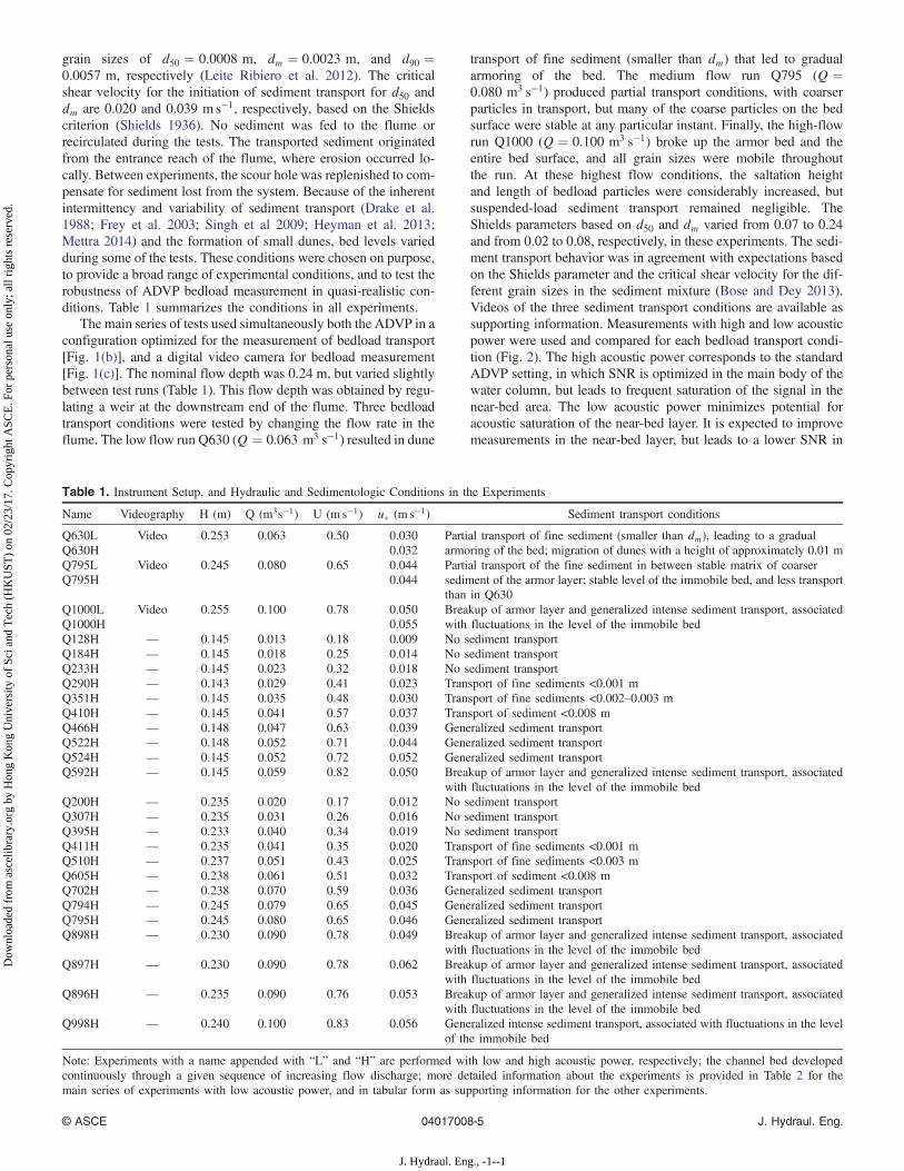
transport, by investigating the physical meaning of the velocitymeasured with the ADVP in the region where bedload sedimenttransport occurs. In all experiments without sediment transport re-ported in this paper, the ADVP resolved the law of the wall log-arithmic velocity profile, including very close to the bed [Fig. 3(a)].On the contrary, in all experiments with bedload sediment trans-port reported in this paper, velocities in the near-bed region wherebedload sediment transport occurs were found to deviate from thelogarithmic profile [Figs. 3(a and b)], similar to observations ofNaqshband et al. (2014b). The main hypothesis of the present paperis that the ADVP measures the velocity of the sediment particlesmoving as bedload in this near-bed region. The hypothesis is testedover a range of bedload transport conditions for a gravel-sand bedmaterial mixture in a mobile bed flume. In this paper we focus onmeasurement of bedload particle velocities and the thickness of thebed load layer. To validate the hypothesis, three strategies are fol-lowed. First, a detailed analysis is performed of the raw IðtÞ andQðtÞ signals recorded by the ADVP’s receivers that reveals a clearfootprint of the bedload sediment particles. Second, simultaneousobservations of bedload sediment transport are conducted withhigh-speed digital videography. Third, ADVP-based estimates ofthe bedload velocities and thickness of the bedload layer are com-pared with semitheoretical formulas based on previous results.

The present research makes use of an ADVP configuration thatis specifically designed and tested for measurement of bedloadtransport. As described subsequently, the instrument beam geom-etry is designed such that it is most sensitive in the first bin abovethe bed, and the acoustic power is chosen such that backscatteredsignal remains within the recording range of the receivers in thebedload region (Fig. 2). The bedload measurement capabilities ofthis optimized ADVP configuration and the standard ADVP con-figuration for flow measurements are also compared.

Methods

Experimental Program

The ADVP’s potential to measure bedload was tested in a flume atÉcole Polytechnique Fédéral de Lausanne (EPFL). The flume was0.50 m wide with zero slope, and the test section was 6.6 m down-stream of the flume inlet. The bed sediment was poorly sorted[σ ¼ 0.5 × ðd84=d50 þ d50=d16Þ ¼ 4.15, where di represents theith percentile grain size] with median, mean, and 90th-percentile

Water surface

0 10 20 30 40 50 60 7060

55

50

45

40

35

30

25

20

AD

VP

Bin

num

ber

0

0.02

0.04

0.06

0.08

0.1

0.12

0.14

0.16

Magnitude backscattered acoustic signal

Dis

tanc

e ab

ove

imm

obile

bed

[m

]

Top rolling and sliding bedload layer

Outside sensitivityrange ADVP receivers

Immobile bed surface

Top saltating bedload layer

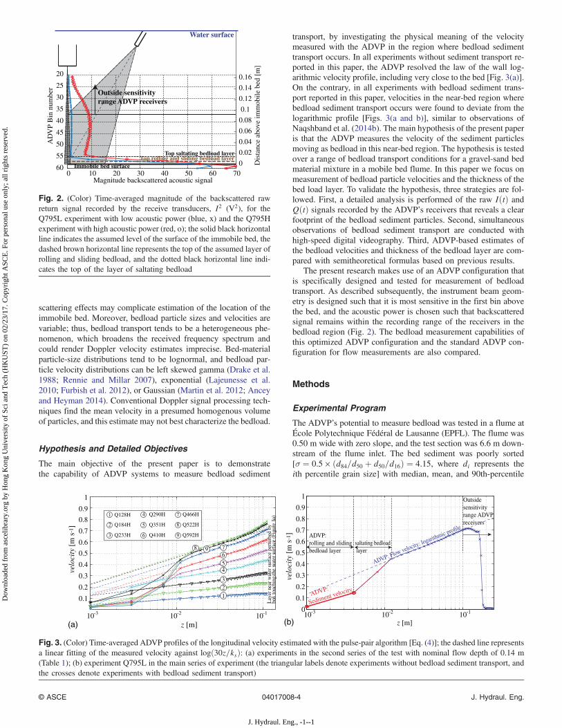
Fig. 2. (Color) Time-averaged magnitude of the backscattered rawreturn signal recorded by the receive transducers, I2 (V2), for theQ795L experiment with low acoustic power (blue, x) and the Q795Hexperiment with high acoustic power (red, o); the solid black horizontalline indicates the assumed level of the surface of the immobile bed, thedashed brown horizontal line represents the top of the assumed layer ofrolling and sliding bedload, and the dotted black horizontal line indi-cates the top of the layer of saltating bedload

ADVP: Flow velocity: logarithmic profile

ADVP:

Sediment velocity

ADVP: rolling and slidingbedload layer

Outsidesensitivityrange ADVPreceivers

saltating bedload layer

10-3 10-2 10-10

0.1

0.2

0.3

0.4

0.5

0.6

0.7

0.8

0.9

1

z [m]

velo

city

[m

s-1

]

Lay

er n

ear w

ater

sur

face

per

turb

ed b

y bo

x to

uchi

ng th

e w

ater

sur

face

(Fig

ure

1a)

10-3 10-2 10-1

0.1

0.2

0.3

0.4

0.5

0.6

0.7

0.8

0.9

1

z [m](a) (b)

velo

city

[m

s-1

]

Q128H

Q184H

Q233H

Q290H

Q351H

Q410H

Q466H

Q522H

Q592H

1

2

3

4

5

6

7

8

9

123

45678 9

Fig. 3. (Color) Time-averaged ADVP profiles of the longitudinal velocity estimated with the pulse-pair algorithm [Eq. (4)]; the dashed line representsa linear fitting of the measured velocity against logð30z=ksÞ: (a) experiments in the second series of the test with nominal flow depth of 0.14 m(Table 1); (b) experiment Q795L in the main series of experiment (the triangular labels denote experiments without bedload sediment transport, andthe crosses denote experiments with bedload sediment transport)



Dow

nloa

ded

from

asc

elib

rary

.org

by

Hon

g K

ong

Uni

vers

ity o

f Sc

i and

Tec

h (H

KU

ST)

on 0

2/23

/17.

Cop

yrig

ht A

SCE

. For

per

sona

l use

onl

y; a

ll ri

ghts

res

erve

d.

grain sizes of d50 ¼ 0.0008 m, dm ¼ 0.0023 m, and d90 ¼0.0057 m, respectively (Leite Ribiero et al. 2012). The criticalshear velocity for the initiation of sediment transport for d50 anddm are 0.020 and 0.039 ms−1, respectively, based on the Shieldscriterion (Shields 1936). No sediment was fed to the flume orrecirculated during the tests. The transported sediment originatedfrom the entrance reach of the flume, where erosion occurred lo-cally. Between experiments, the scour hole was replenished to com-pensate for sediment lost from the system. Because of the inherentintermittency and variability of sediment transport (Drake et al.1988; Frey et al. 2003; Singh et al 2009; Heyman et al. 2013;Mettra 2014) and the formation of small dunes, bed levels variedduring some of the tests. These conditions were chosen on purpose,to provide a broad range of experimental conditions, and to test therobustness of ADVP bedload measurement in quasi-realistic con-ditions. Table 1 summarizes the conditions in all experiments.

The main series of tests used simultaneously both the ADVP in aconfiguration optimized for the measurement of bedload transport[Fig. 1(b)], and a digital video camera for bedload measurement[Fig. 1(c)]. The nominal flow depth was 0.24 m, but varied slightlybetween test runs (Table 1). This flow depth was obtained by regu-lating a weir at the downstream end of the flume. Three bedloadtransport conditions were tested by changing the flow rate in theflume. The low flow run Q630 (Q ¼ 0.063 m3 s−1) resulted in dune

transport of fine sediment (smaller than dm) that led to gradualarmoring of the bed. The medium flow run Q795 (Q ¼0.080 m3 s−1) produced partial transport conditions, with coarserparticles in transport, but many of the coarse particles on the bedsurface were stable at any particular instant. Finally, the high-flowrun Q1000 (Q ¼ 0.100 m3 s−1) broke up the armor bed and theentire bed surface, and all grain sizes were mobile throughoutthe run. At these highest flow conditions, the saltation heightand length of bedload particles were considerably increased, butsuspended-load sediment transport remained negligible. TheShields parameters based on d50 and dm varied from 0.07 to 0.24and from 0.02 to 0.08, respectively, in these experiments. The sedi-ment transport behavior was in agreement with expectations basedon the Shields parameter and the critical shear velocity for the dif-ferent grain sizes in the sediment mixture (Bose and Dey 2013).Videos of the three sediment transport conditions are available assupporting information. Measurements with high and low acousticpower were used and compared for each bedload transport condi-tion (Fig. 2). The high acoustic power corresponds to the standardADVP setting, in which SNR is optimized in the main body of thewater column, but leads to frequent saturation of the signal in thenear-bed area. The low acoustic power minimizes potential foracoustic saturation of the near-bed layer. It is expected to improvemeasurements in the near-bed layer, but leads to a lower SNR in

Table 1. Instrument Setup, and Hydraulic and Sedimentologic Conditions in the Experiments

Name Videography H (m) Q (m3s−1) U (m s−1) u� (m s−1) Sediment transport conditions

Q630L Video 0.253 0.063 0.50 0.030 Partial transport of fine sediment (smaller than dm), leading to a gradualarmoring of the bed; migration of dunes with a height of approximately 0.01 mQ630H 0.032

Q795L Video 0.245 0.080 0.65 0.044 Partial transport of the fine sediment in between stable matrix of coarsersediment of the armor layer; stable level of the immobile bed, and less transportthan in Q630

Q795H 0.044

Q1000L Video 0.255 0.100 0.78 0.050 Breakup of armor layer and generalized intense sediment transport, associatedwith fluctuations in the level of the immobile bedQ1000H 0.055

Q128H — 0.145 0.013 0.18 0.009 No sediment transportQ184H — 0.145 0.018 0.25 0.014 No sediment transportQ233H — 0.145 0.023 0.32 0.018 No sediment transportQ290H — 0.143 0.029 0.41 0.023 Transport of fine sediments <0.001 mQ351H — 0.145 0.035 0.48 0.030 Transport of fine sediments <0.002–0.003 mQ410H — 0.145 0.041 0.57 0.037 Transport of sediment <0.008 mQ466H — 0.148 0.047 0.63 0.039 Generalized sediment transportQ522H — 0.148 0.052 0.71 0.044 Generalized sediment transportQ524H — 0.145 0.052 0.72 0.052 Generalized sediment transportQ592H — 0.145 0.059 0.82 0.050 Breakup of armor layer and generalized intense sediment transport, associated

with fluctuations in the level of the immobile bedQ200H — 0.235 0.020 0.17 0.012 No sediment transportQ307H — 0.235 0.031 0.26 0.016 No sediment transportQ395H — 0.233 0.040 0.34 0.019 No sediment transportQ411H — 0.235 0.041 0.35 0.020 Transport of fine sediments <0.001 mQ510H — 0.237 0.051 0.43 0.025 Transport of fine sediments <0.003 mQ605H — 0.238 0.061 0.51 0.032 Transport of sediment <0.008 mQ702H — 0.238 0.070 0.59 0.036 Generalized sediment transportQ794H — 0.245 0.079 0.65 0.045 Generalized sediment transportQ795H — 0.245 0.080 0.65 0.046 Generalized sediment transportQ898H — 0.230 0.090 0.78 0.049 Breakup of armor layer and generalized intense sediment transport, associated

with fluctuations in the level of the immobile bedQ897H — 0.230 0.090 0.78 0.062 Breakup of armor layer and generalized intense sediment transport, associated

with fluctuations in the level of the immobile bedQ896H — 0.235 0.090 0.76 0.053 Breakup of armor layer and generalized intense sediment transport, associated

with fluctuations in the level of the immobile bedQ998H — 0.240 0.100 0.83 0.056 Generalized intense sediment transport, associated with fluctuations in the level

of the immobile bed

Note: Experiments with a name appended with “L” and “H” are performed with low and high acoustic power, respectively; the channel bed developedcontinuously through a given sequence of increasing flow discharge; more detailed information about the experiments is provided in Table 2 for themain series of experiments with low acoustic power, and in tabular form as supporting information for the other experiments.



Dow

nloa

ded

from

asc

elib

rary

.org

by

Hon

g K

ong

Uni

vers

ity o

f Sc

i and

Tec

h (H

KU

ST)

on 0

2/23

/17.

Cop

yrig

ht A

SCE

. For

per

sona

l use

onl

y; a

ll ri

ghts

res

erve

d.

the main body of the water column. The labels of experimentswith high and low acoustic power are appended with H and L,respectively (Table 1).

A second series of tests was also collected with the ADVP in itsstandard configuration optimized for flow measurements in thebody of the water column [Fig. 1(a)], and without simultaneousvideography (Table 1). The purpose of this series was to comparethe capabilities of the standard ADVP configuration and the oneoptimized for bedload measurements, and to extend the investiga-tion to a broader range of hydraulic conditions. Experiments wereperformed with nominal flow depths of 0.14 and 0.24 m. For eachof these flow depths, 10 different discharges were tested (Table 1).In the tests with 0.14-m flow depth, discharge ranged from 0.013 to0.060 m3 s−1, shear velocity from 0.009 to 0.052 ms−1, and theShields parameters based on d50 and dm from 0.006 to 0.20 andfrom 0.002 to 0.07, respectively. In the tests with 0.24-m flowdepth, discharge ranged from 0.020 to 0.100 m3 s−1, shear velocityfrom 0.012 to 0.062 ms−1, and the Shields parameter based on d50and dm from 0.01 to 0.29 and from 0.003 to 0.10, respectively. Atthe lowest discharge, no sediment transport occurred, whereas gen-eralized and intense sediment transport occurred at the highestdischarge. Again, the sediment transport behavior was as expectedbased on the Shields parameter and the critical shear velocity forthe different grain sizes in the bed mixture (Bose and Dey 2013).The runs with 0.24-m flow depth encompassed the hydraulicconditions investigated in the main series with optimized ADVPconfiguration and simultaneous videography, which facilitatescomparison.

ADVP Configuration and Data Analysis Procedures

The ADVP used for this research has been developed at EPFL.Its working principle has been detailed in Rolland and Lemmin(1997), Hurther and Lemmin (1998, 2001), Hurther (2001), andBlanckaert and Lemmin (2006). The instrument consists of a cen-tral emit transducer of diameter 0.034 m and of carrier frequencyf0 ¼ 1 MHz, with beam width of 1.7°, and four 30° fan-beam re-ceive transducers that are 30° inclined from the vertical (Fig. 1).In all experiments, PRF was set to 1,000 Hz, and NPP to 32, yield-ing a sampling frequency of PRF=NPP ¼ 31.25 Hz for the quasi-instantaneous Doppler frequencies and velocities. A pulse lengthof 5 μs was chosen, yielding a vertical resolution of velocity binsof approximately 0.004 m. A time series of more than 10 min wascollected for each test condition, which was sufficient to obtain stat-istically stable measurements of the flow and sediment transportunder quasi-steady conditions. Blanckaert and de Vriend (2004)and Blanckaert (2010) discuss in detail the uncertainty in the flowquantities measured with this ADVP. They report a conservativeestimate of 4% uncertainty in the streamwise velocity u.

In the main series of tests (Table 1), the ADVP configurationwas optimized to measure bedload transport, as explained hereafter[Fig. 1(b)]. The ADVP was configured symmetrically, with hori-zontal and vertical distances between emit and receive transducersof 0.1305 and 0.0304 m, respectively. The ADVP was immersed inthe flow, with the emit transducer 0.185 m above the nominal bedlevel. With this configuration, the center of the receive beam wasfocused on the bed level. This ensured that the ADVP was mostsensitive in the vicinity of the bedload layer. This configuration,however, did not allow for measurements in the upper half of thewater column [Fig. 1(b)].

In the second series of experiments (Table 1), the standardADVP configuration was used [Fig. 1(a)]. Receivers symmetricallysurrounded the emit transducer at horizontal and vertical distancesof 0.1343 and 0.0295 m, respectively. To measure the entire water

column, the ADVP was placed approximately 7 cm above the watersurface in a water-filled box that was separated from the flowingwater with an acoustically transparent Mylar film (DuPont TeijinFilms, Chester, Virginia) [Fig. 1(a)]. The box induces perturbationsof the flow in a layer with a thickness of approximately 0.02 mnear the water surface. In the experiments with flow depth of0.14 m, the center of the receive beam was focused on the bed level.In the experiments with flow depth of 0.24 m, it was focused in thecore of the water column, approximately 0.10 m above the bed[Fig. 1(a)].

The acoustic footprint on the bed of the emitted beam is circularwith a diameter that ranges from approximately 0.045 m in the ex-periments with 0.14-m flow depth to approximately 0.055 m in theexperiments with 0.24-m flow depth (Fig. 1). This indicates that theADVP does not resolve grain scale processes, but processes at acharacteristic scale of approximately 0.05 m.

The standard ADVP data analysis procedure considers two out-put quantities: the magnitude of the backscattered signal recordedby the receive transducers (Fig. 2), and the time-averaged velocityestimated with the pulse-pair algorithm [Eq. (4), Fig. 3].

The profile of the time-averaged longitudinal flow velocity istypically logarithmic in the vicinity of the bed in cases without bed-load sediment transport (Nezu and Nakagawa 1993). To identifythe logarithmic part, the measured time-averaged velocity is plottedas a function of logð30z=ksÞ, in which z is the distance in metersabove the immobile bed, and the equivalent grain roughness ks istaken as 0.01 m (Fig. 3). To avoid singularities, the bin containingthe surface of the immobile bed has been plotted at z ¼ 0.001 m.The profile of the time-averaged velocity as a function oflogð30z=ksÞ also identifies the near-bed region where the measuredvelocities are smaller than the logarithmic profile in cases with bed-load sediment transport, similar to observations by Naqshband et al.(2014b). In this nonlogarithmic near-bed layer, the measured veloc-ity profiles typically have an S-shape (Fig. 3). As mentioned pre-viously, the main hypothesis of the present paper is that the ADVPmeasures the particle velocities in this near-bed zone. Sediment ispredominantly moving as bed load transport in the investigated ex-periments. Most particles are intermittently entrained from the im-mobile bed by the flow, slide and roll over the immobile bed, andfinally immobilize again. The velocity of these sliding and rollingparticles is generally smaller than the velocity of the surroundingfluid, as a result of momentum extraction by interparticle collisions,inertia of the sediment particles, and friction on the granular bed.The difference between the velocities of particles and the entrainingflow is called the slip velocity (Nino and Garcia 1996; Muste et al.2009). It is assumed that the extrapolated logarithmic profile pro-vides an estimate of the velocity of the entraining flow. An increasein the number of moving particles can be assumed to increase themomentum extraction as a result of interparticle collision, andhence also the slip velocity. Therefore, the dominant bed load trans-port is assumed to occur at the elevation of maximum slip velocity,which approximately coincides with the inflection point in theS-shaped near-bed velocity profile [Fig. 3(b)]. By definition, thisinflection point occurs where the second derivative of the velocitywith respect to z vanishes. Some bedload particles saltate on thebed and reach higher elevations in the water column. Because sal-tating bedload particles are usually relatively small and their salta-tion length scale is longer with fewer interparticle collisions thanthose of the rolling bedload particles, their velocity is closer tothe velocity of the entraining fluid. As mentioned previously, sus-pended load particles have negligible slip velocity and move atabout the same velocity as the flow. Thus, the shape of the mea-sured velocity profile identifies the layer with rolling and sliding



Dow

nloa

ded

from

asc

elib

rary

.org

by

Hon

g K

ong

Uni

vers

ity o

f Sc

i and

Tec

h (H

KU

ST)

on 0

2/23

/17.

Cop

yrig

ht A

SCE

. For

per

sona

l use

onl

y; a

ll ri

ghts

res

erve

d.

bedload transport, the layer with saltating bedload transport, andthe layer with suspended load transport or clear water.

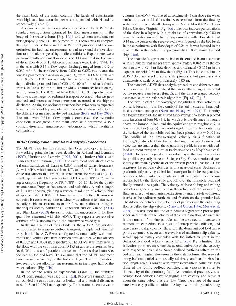
A critical issue in the identification of the different layers ofsediment transport is the identification of the elevation of the sur-face of the immobile bed, which by definition corresponds to zerovelocity. The accuracy in the identification of the immobile bedsurface is limited by the finite bin size of 0.004 m and by the factthat a natural sediment bed is not perfectly planar. The best practiceconsists of identifying the bin in which the surface of the immobilebed is situated, as illustrated in Fig. 4. The upper part of that binwill be situated in the flow. In case no bedload sediment transportoccurs, the ADVP will measure zero velocity in the bin containingthe surface of the immobile bed, because the magnitude of the rawsignal backscattered on micro air bubbles in the flowing water ismuch smaller than the magnitude of the one backscattered on theimmobile bed. If bedload sediment particles roll and slide onthe immobile bed within the bin containing the immobile bed, theADVP will measure a nonzero velocity, which corresponds to theaverage velocity of sediment particles within that bin (Fig. 4)(i.e., this spatial average also includes areas of zero velocity asso-ciated with immobile particles within the measuring area of theADVP). The bin containing the surface of the immobile bed istherefore identified as the bin with the minimum nonzero velocity,as illustrated in Figs. 3 and 4.

A second independent estimation of the bin containing the sur-face of the immobile bed is obtained from the magnitude of the rawbackscattered signal recorded by the receivers, I2 ¼ 0.25 (I21 þI22 þ I23 þ I24) (Fig. 2). Here, I1, I2, I3, and I4 are the raw in-phasecomponents of the demodulated signals recorded by each of thefour receivers. The magnitude of the backscattered signal relates

to the concentration of the sediment particles, because sedimentparticles backscatter considerably more acoustic energy than microair bubbles in the water column above (Hurther et al. 2011). Basedon this heuristic definition, the bin containing the immobile bed isassumed to correspond to the peak in the profile of the magnitudeof the backscattered signal (Fig. 2). In the present paper, we usedthe first estimation to define the bin containing the surface of theimmobile bed, and the second estimation for validation purposes.In general, both estimations identified the same bin.

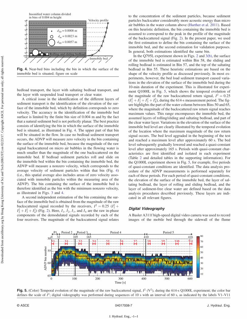
In the Q795L experiment shown in Figs. 2 and 3(b), the surfaceof the immobile bed is estimated within Bin 58, the sliding androlling bedload is estimated in Bin 57, and the top of the saltatingbedload in Bin 55. These heuristic estimations are based on theshape of the velocity profile as discussed previously. In most ex-periments, however, the bed load sediment transport caused varia-tions in the elevation of the surface of the immobile bed during the10-min duration of the experiment. This is illustrated for experi-ment Q1000L in Fig. 5, which shows the temporal evolution ofthe magnitude of the raw backscattered return signal, I2 ¼ 0.25(I21 þ I22 þ I23 þ I24), during the 614-s measurement period. The fig-ure highlights the part of the water column between Bins 50 and 65,where the magnitude of the backscattered raw return signal reachesmaximum values. This range encompasses the immobile bed, theassumed layers of rolling/sliding and saltating bedload, and part ofthe clear water layer. Variations in the elevation of the surface of theimmobile bed level are clearly illustrated by the temporal evolutionof the location where the maximum magnitude of the raw returnsignal occurs. The bed level aggraded in the beginning of the testand reached a maximum level after approximately 60 s. The bedlevel subsequently gradually lowered and reached a quasi-constantlevel after approximately 165 s. Periods with quasi-constant char-acteristics are first identified and isolated in each experiment(Table 2 and detailed tables in the supporting information). Forthe Q1000L experiment shown in Fig. 5, for example, five periodsof quasi-constant conditions are identified. The data analysis pro-cedure of the ADVP measurements is performed separately foreach of these periods. For each period of quasi-constant conditions,the elevation of the surface of the immobile bed, the layer of sal-tating bedload, the layer of rolling and sliding bedload, and thelayer of sediment-free clear water are defined based on the dataanalysis procedures described previously. These layers are indi-cated in all relevant figures.

Digital Videography

A Basler A311f high-speed digital video camera was used to recordimages of the mobile bed through the sidewall of the flume

d50 = 0.0008 m

dm = 0.0023 m

d90 = 0.0057 m

Insonified water column dividedin bins of 0.004 m height

Velocity profile

Immobile bedRolling and sliding bedload

Fig. 4. Near-bed bins including the bin in which the surface of theimmobile bed is situated; figure on scale

100 200 300 400 500 600

50

55

60

65

Time [s]

AD

VP

bin

num

ber

0

0 32 105 165 410 416

Period 5Period 4Period 3Period 2P1

V1 V11V10V9V8V7V6V5V4V3V2

10

20

30

40

50

60

70

80

Fig. 5. (Color) Temporal evolution of the magnitude of the raw backscattered signal, I2 (V2), during the 614-s Q1000L experiment; the color bardefines the scale of I2; digital videography was performed during sequences of 10 s with an interval of 60 s, as indicated by the labels V1–V11



Dow

nloa

ded

from

asc

elib

rary

.org

by

Hon

g K

ong

Uni

vers

ity o

f Sc

i and

Tec

h (H

KU

ST)

on 0

2/23

/17.

Cop

yrig

ht A

SCE

. For

per

sona

l use

onl

y; a

ll ri

ghts

res

erve

d.

[Fig. 1(c)]. The images gave a distorted picture of the bed (as aresult of perspective) but were centered on the ADVP samplevolume in the center of the flume, with a 0.122-m centerline lon-gitudinal by 0.155-m transverse field of view. The images had656 × 300 resolution; thus, the pixel size was approximately0.0002 × 0.0005 m. The videography maps the three-dimensionalsediment motion on a horizontal plane, which is complementary tothe resolution in a vertical water column provided by the ADVP.Image exposure time was 300 μs, and sampling rate was 111 Hz.Computer clock times were used to synchronize image acquis-ition with ADVP data collection. Digital video images were orthor-ectified using a projective transformation (Beutelspacher andRosenbaum 1998). Because of limitations in computer storageand data transfer, digital videos with high temporal resolution couldonly be recorded for a maximum of 10 s. During the 10-min ADVPdata collection, 10-s digital videos were collected once everyminute (Fig. 5). The cumulative duration of the digital videos ofmore than 110 s is long enough to obtain reliable estimates ofthe velocities of the bedload particles. Two complementary imagetreatment algorithms were used.

To estimate the velocity of sediment particles, the robust open-source particle tracking velocimetry (PTV) algorithm PolyParticle-Tracker was used (Rogers et al. 2007). This algorithm is able toestimate the position and track several objects through frames witha subpixel resolution. The algorithm was specifically developed fortracking bright objects over a complex background. The particle

instantaneous velocities are then estimated by time differentiationof the particle positions. Erroneous trajectories were filtered withtechniques commonly used in particle image velocimetry. First, amaximum acceleration criterion of 40 ms−2 was defined for indi-vidual particles. Then, the angle between two successive velocityvectors was limited to 90°. Particles are often found with velocitiesclose to zero while bouncing on the bed. To avoid sampling of thesequasi-immobile bed particles that only marginally contribute tothe sediment flux, a minimum velocity threshold of 0.04 ms−1 wasadopted. Full trajectories of particles, from entrainment to deposi-tion, were not always recovered by the algorithm, primarily be-cause of the presence of the noisy background consisting ofresting particles. Moreover, not all of the moving particles weresystematically detected. It can be expected that especially the sal-tating bedload with relatively small grain size and relatively highvelocities was undersampled. Enough particle trajectories were cor-rectly recovered to provide a good estimate of the distribution func-tions of the sediment velocities and the time-averaged velocity ofthe moving sediment particles. These quantities will be shown anddiscussed in the “Simultaneous Videography” section.

An instantaneous spatio-temporal quantification of the bedloadlayer velocities, however, was not possible from the trajectories ob-tained with the PTV method, as not all of the moving particles weresystematically detected by the automated algorithm, and becausefull trajectories from entrainment to deposition were not alwaysrecovered. To estimate bedload velocity time series in the ADVP

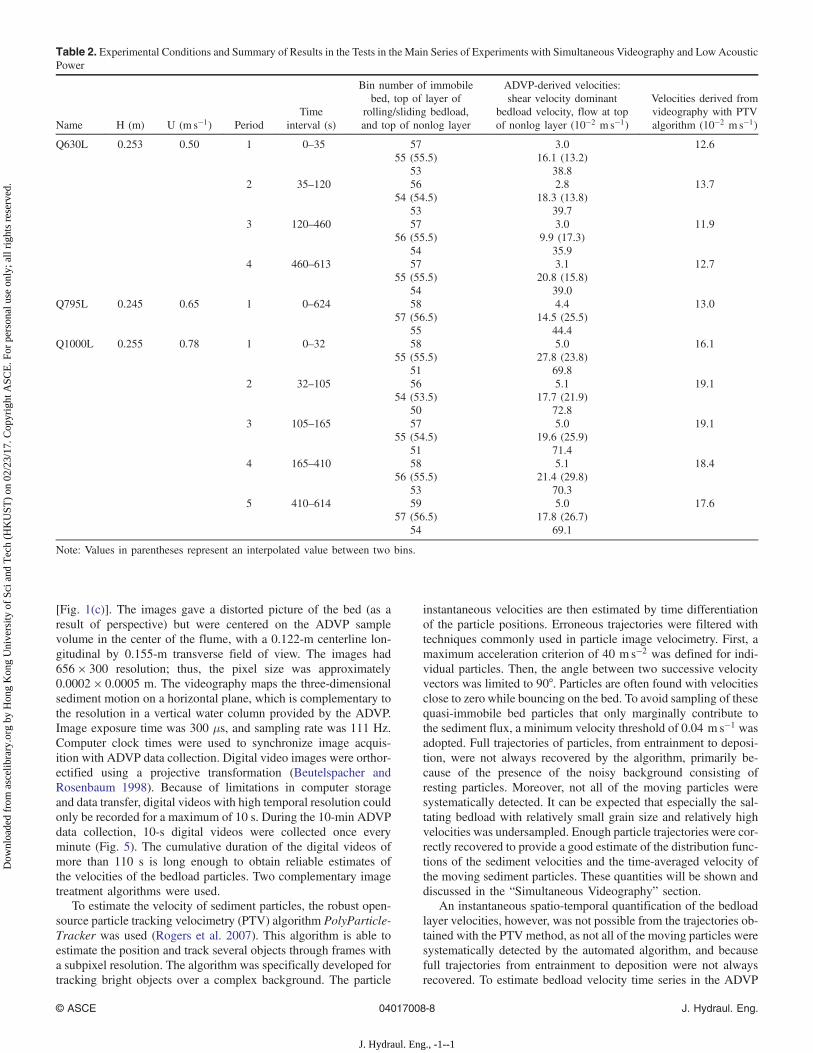
Table 2. Experimental Conditions and Summary of Results in the Tests in the Main Series of Experiments with Simultaneous Videography and Low AcousticPower

Name H (m) U (m s−1) PeriodTime

interval (s)

Bin number of immobilebed, top of layer of

rolling/sliding bedload,and top of nonlog layer

ADVP-derived velocities:shear velocity dominant

bedload velocity, flow at topof nonlog layer (10−2 ms−1)

Velocities derived fromvideography with PTValgorithm (10−2 ms−1)

Q630L 0.253 0.50 1 0–35 57 3.0 12.655 (55.5) 16.1 (13.2)

53 38.82 35–120 56 2.8 13.7

54 (54.5) 18.3 (13.8)53 39.7

3 120–460 57 3.0 11.956 (55.5) 9.9 (17.3)

54 35.94 460–613 57 3.1 12.7

55 (55.5) 20.8 (15.8)54 39.0

Q795L 0.245 0.65 1 0–624 58 4.4 13.057 (56.5) 14.5 (25.5)

55 44.4Q1000L 0.255 0.78 1 0–32 58 5.0 16.1

55 (55.5) 27.8 (23.8)51 69.8

2 32–105 56 5.1 19.154 (53.5) 17.7 (21.9)

50 72.83 105–165 57 5.0 19.1

55 (54.5) 19.6 (25.9)51 71.4

4 165–410 58 5.1 18.456 (55.5) 21.4 (29.8)

53 70.35 410–614 59 5.0 17.6

57 (56.5) 17.8 (26.7)54 69.1

Note: Values in parentheses represent an interpolated value between two bins.



Dow

nloa

ded

from

asc

elib

rary

.org

by

Hon

g K

ong

Uni

vers

ity o

f Sc

i and

Tec

h (H

KU

ST)

on 0

2/23

/17.

Cop

yrig

ht A

SCE

. For

per

sona

l use

onl

y; a

ll ri

ghts

res

erve

d.

sample volume, a complementary analysis of the digital videoimages was performed with the optical flow algorithm (Horn andSchunck 1981). This algorithm remediates the small sample limi-tation of the particle tracking algorithm by computing for each pairof frames a dense two-dimensional velocity field that reflects thelocal apparent motion in the image. The algorithm assumes that theintensity value Iðx; y; tÞ of each pixel follows a simple advectionequation as follows:

∂I∂t þ u

∂I∂xþ v

∂I∂y ¼ ε ð5Þ

where the problem unknowns are the velocity components uðx; y; tÞand vðx; y; tÞ along the x- and y-axes. The partial derivatives of Ican be estimated directly from the video stream: ∂I=∂t is the tem-poral change in pixel intensity, and ∂I=∂x and ∂I=∂y are the spatialgradients in pixel intensity. The optical flow method determines thevelocity field (u; v), which minimizes ε. Intuitively, the apparentmotion of an object is better appreciated by the human eye if itcontains high-intensity gradients (border contrasts for instance).In contrast, the motion of objects with low contrast is difficultto estimate by the human eye. This is similar for the optical flowmethod, which will perform better when ∂I=∂x and ∂I=∂y arelarger. In case these spatial gradients equal zero, the velocity field(u; v) is not uniquely determined by Eq. (5) and the problem is ill-posed. In this case, an additional constraint [also called a regular-izer (Horn and Schunck 1981)] needs to be imposed, usually basedon the continuity of the velocity field. The efficiency of this tech-nique therefore relies on the presence of strong intensity gradients,as those frequently observed at object edge contours. The opticalflow algorithm can be expected to be especially appropriate for thelargest bedload particles that roll and slide on the immobile bed,because these particles form well-distinguishable contours in thedigital images that yield large gradients ∂I=∂x and ∂I=∂y. Fasterand smaller bedload particles can be expected to be undersampledas a result of their weaker intensity gradients. This algorithmhas been applied successfully in numerous applications, includingflow reconstruction from particle image velocimetry techniques(Ruhnau et al. 2005; Heitz et al. 2008), but it has rarely been ap-plied to the estimation of sediment motion (Spies et al. 1999; Klaret al. 2004). In this study, the optical flow algorithm has been ap-plied to investigate the time-resolved velocity of the bedload par-ticles inside the ADVP sample volume. The particle velocities havebeen estimated from the digital video images with the open accessMATLAB implementation of the Lukas-Kanade method (Lucas andKanade 1981) by Stefan M. Karlsson and Josef Bigun and availableat http://www.mathworks.com/matlabcentral/fileexchange/40968.To improve the accuracy and to reduce noise, the velocity fieldwas averaged on a 70 × 70 grid overlapping the original 656 ×300 pixel images. The local sediment velocity that was spatiallyaveraged within the footprint of the ADVP’s measuring beam atthe bed was then obtained by averaging the 70 × 70 optical flowvelocity field using a Gaussian kernel centered on the volume. Thisspatial average also includes areas of zero velocity associated withimmobile particles, and thus reflects the average bed velocity. Thisis different from the sediment velocities estimated with the PTValgorithm, which considers only the moving sediment particles.It is similar, however, to the velocities measured by the ADVPin the bin containing the surface of the immobile bed (see “ADVPConfiguration and Data Analysis Procedures” section). The tempo-ral fluctuations of this locally spatially averaged velocity willbe shown and discussed in the “Simultaneous Videography”section.

Results

Signature of the Raw Signals Recorded by the ADVP

Most commercial ADVP systems provide as output only the quasi-instantaneous Doppler frequencies or velocities sampled at PRF/NPP. The ADVP used in the present investigation also providesthe backscattered raw return signals recorded by the receivers, Iand Q, sampled at PRF. This is a major advantage, as it allowsthe analysis of raw signals for the presence of a footprint of bedloadsediment transport. This analysis will be illustrated for the Q795Lexperiment, in which the bed level remained stable during the entire624 s of continuous measurements.

First, the time-averaged magnitude of the backscattered raw re-turn signal, I2 ¼ 0.25 (I21 þ I22 þ I23 þ I24) is considered (Fig. 2).The magnitude of the backscattered signal relates to the concentra-tion of the sediment particles, because sediment particles backscat-ter considerably more acoustic energy than micro air bubbles in thewater column above (Hurther et al. 2011). The magnitude of thereturn signal decreases with distance upward from the immobilebed level, which complies with the expectation that sediment con-centration decreases with distance from the immobile bed. Wehypothesize that the bins with considerably increased magnitudeof the return signal correspond to the layer of rolling and slidingbedload sediment, and that bins characterized by the base level ofacoustic backscatter magnitude correspond to clear water flow.Bins in between the rolling and sliding bedload transport layerand the clear-water flow layer are assumed to correspond to saltat-ing bedload.

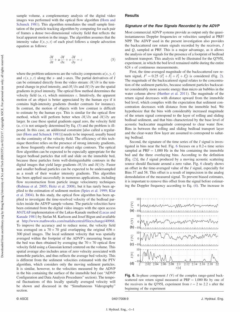
Second, the signature of the time series of the I signal is inves-tigated in bins near the bed. Fig. 6 focuses on a 0.2-s time seriessampled at PRF ¼ 1,000 Hz in the bin containing the immobilebed and the three overlaying bins. According to the definition[Eq. (2)], the I signal produced by a moving acoustic scatteringsource should fluctuate around a zero value. Fig. 6 clearly showsan offset in the time-averaged value of the I signal, especially forBins 57 and 58. This offset is a result of imprecision in the analogdemodulation of the measured signal. To prevent biased estimates,it is important to remove this offset from the signal before estimat-ing the Doppler frequency according to Eq. (4). The increase in

−10

0

10

−10

0

10

−10

0

10

2 2.02 2.04 2.06 2.08 2.1 2.12 2.14 2.16 2.18 2.2−10

0

10

t [s]

I [V

]I

[V]

I [V

]I

[V]

(a)

(b)

(c)

(d)

Fig. 6. In-phase component I (V) of the complex range-gated back-scattered raw return signal measured at PRF ¼ 1,000 Hz by one ofthe receivers in the Q795L experiment from t ¼ 2 to 2.2 s after thebeginning of the experiment



Dow

nloa

ded

from

asc

elib

rary

.org

by

Hon

g K

ong

Uni

vers

ity o

f Sc

i and

Tec

h (H

KU

ST)

on 0

2/23

/17.

Cop

yrig

ht A

SCE

. For

per

sona

l use

onl

y; a

ll ri

ghts

res

erve

d.

http://www.mathworks.com/matlabcentral/fileexchange/40968

magnitude of the raw return signal toward the bed observed in Fig. 2can be recognized in the increasing amplitude of the I fluctuationstoward the bed in Fig. 6. The I signal in Bin 55 shows oscillationswith a frequency and amplitude that varies in time, as can be ex-pected for flow velocities in clear water. According to Hurther andThorne (2011) and Naqshband et al. (2014b), the zero velocity andhighest sediment concentration at the immobile bed surface, esti-mated within Bin 58, should in theory correspond to a constant Ivalue of high amplitude with negligible variance. Fig. 6 shows thatthe measured amplitude is not always constant, but that sequencesof fluctuating voltage occur. These sequences represent the inter-mittent passage of bedload particles that roll and slide on the im-mobile bed (Fig. 4) (see “ADVP Configuration and Data AnalysisProcedures” section).

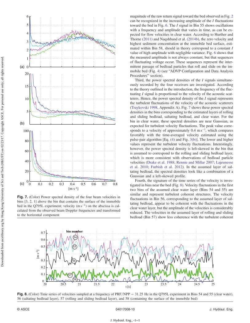
Third, the power spectral densities of the I signals simultane-ously recorded by the four receivers are investigated. Accordingto the theory outlined in the introduction, the frequency of the fluc-tuating I signal is proportional to the velocity of the acoustic scat-terers. Hence, the power spectral density of the I signal representsthe turbulent fluctuations of the velocity of the acoustic scatterers(Traykovski 1998, Appendix A). Fig. 7 shows these power spectraldensities in the bins corresponding to the estimated layers of rollingand sliding bedload, saltating bedload, and clear water. For thebin in clear water, these spectral densities are near Gaussian, asexpected for turbulent velocity fluctuations. The peak value corre-sponds to a velocity of approximately 0.4 ms−1, which comparesfavorably with the time-averaged velocity estimated using thepulse-pair algorithm [Eq. (4) and Fig. 3(b)]. The lower and highervalues represent the turbulent velocity fluctuations. Interestingly,however, the power spectral density is left-skewed in the bin thatis assumed to correspond to the rolling and sliding bedload layer,which is more consistent with observations of bedload particlevelocities (Drake et al. 1988; Rennie and Millar 2007; Lajeunesseet al. 2010; Furbish et al. 2012). In the assumed layer of sal-tating bedload, the spectral densities look like a combination of aGaussian and a left-skewed profile.

Fourth, the signature of the time series of the velocity is inves-tigated in bins near the bed (Fig. 8). Velocity fluctuations in the firsttwo bins of the assumed clear water layer (Bins 54 and 55) aresimilar and represent turbulent coherent structures. The velocityfluctuations in Bin 56, corresponding to the assumed layer of sal-tating bedload, appear to be coherent with the fluctuations in theclear water layer, but the amplitude of the velocities is considerablyreduced. The velocities in the assumed layer of rolling and slidingbedload (Bin 57) show less coherence with the turbulent coherent

0

1

2

3

4

5

6

5

10

15

20

0 0.1 0.2 0.3 0.4 0.5 0.6 0.7 0.80

20

40

60

80

100

[m s-1]

(a)

(b)

(c)

Fig. 7. (Color) Power spectral density of the four beam velocities inbins [3, 2, 1] above the bin that contains the surface of the immobilebed in the Q795L experiment; velocity (m s−1) on the abscissa is cal-culated from the observed beam Doppler frequencies and transformedto the horizontal component

20 20.5 21 21.5 22 23 23.5 24 24.5 250

0.1

0.2

0.3

0.5

0.6

0.7

[m s

-1]

t [s]

bin number

54

55

56

5758

Fig. 8. (Color) Time series of velocities sampled at a frequency of PRF=NPP ¼ 31.25 Hz in the Q795L experiment in Bins 54 and 55 (clear water),56 (saltating bedload layer), 57 (rolling and sliding bedload layer), and 58 (containing the surface of the immobile bed)



Dow

nloa

ded

from

asc

elib

rary

.org

by

Hon

g K

ong

Uni

vers

ity o

f Sc

i and

Tec

h (H

KU

ST)

on 0

2/23

/17.

Cop

yrig

ht A

SCE

. For

per

sona

l use

onl

y; a

ll ri

ghts

res

erve

d.

structures in the clear water above. The velocity is considerablysmaller in Bin 58 containing the immobile bed surface. The non-zero velocities represent the intermittent passage of bedload par-ticles that roll and slide on the immobile bed (Fig. 4) (see “ADVPConfiguration and Data Analysis Procedures” section).

A similar analysis of the characteristics of the backscattered rawreturn signal I (Figs. 2, 6, and 7) and the time series of the velocities(Fig. 8) has been performed for all experiments. This analysis re-vealed a clear footprint of the bedload sediment transport in the rawreturn signals, which indicates that the moving bedload sedimentgrains are the main scattering sources. Because the ADVP mea-sures the velocity of the scattering sources, this analysis providesa first indication that the velocities measured by the ADVP corre-spond to the velocities of the moving sediment particles. Moreover,this analysis corroborated the identification based on the profile ofthe time-averaged velocity [Fig. 3(b)] of the bin containing the

immobile-bed surface, the layer of rolling and sliding bedload, andthe layer of saltating bedload.

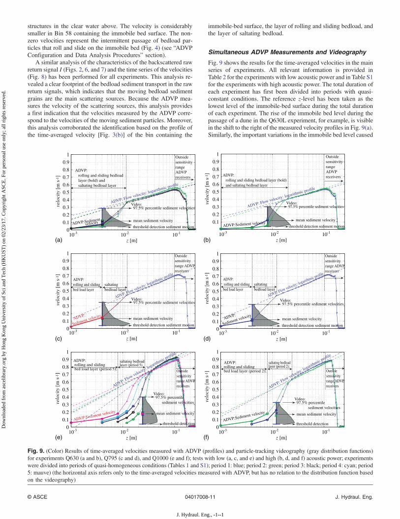
Simultaneous ADVP Measurements and Videography

Fig. 9 shows the results for the time-averaged velocities in the mainseries of experiments. All relevant information is provided inTable 2 for the experiments with low acoustic power and in Table S1for the experiments with high acoustic power. The total duration ofeach experiment has first been divided into periods with quasi-constant conditions. The reference z-level has been taken as thelowest level of the immobile-bed surface during the total durationof each experiment. The rise of the immobile bed level during thepassage of a dune in the Q630L experiment, for example, is visiblein the shift to the right of the measured velocity profiles in Fig. 9(a).Similarly, the important variations in the immobile bed level caused

ADVP: Flow velocity: logarith

mic profile

ADVP:Sediment velocity

ADVP:rolling and slidingbed load layer (period 2); Outside

sensitivityrange ADVPreceivers

saltating bedloadlayer (period 2);

10-3 10-2 10-10

0.1

0.2

0.3

0.4

0.5

0.6

0.7

0.8

0.9

1

z [m]

velo

city

[m

s-1

]

mean sediment velocity

97.5% percentile sediment velocities

threshold detection

Video:


ADVP:Sediment

velocity

ADVP: rolling and sliding bedload layer (bold) and saltating bedload layer



threshold detection sediment motion

OutsidesensitivityrangeADVPreceivers

Video:

10-3 10-2 10-10

0.1

0.2

0.3

0.4

0.5

0.6

0.7

0.8

0.9

1

z [m]

velo

city

[m

s-1

]



OutsidesensitivityrangeADVPreceivers

10-3 10-2 10-1

0.1

0.2

0.3

0.4

0.5

0.6

0.7

0.8

0.9

1

z [m]

velo

city

[m

s-1

]




Video:

ADVP: rolling and sliding bedload layer (bold) and saltating bedload layer


ADVP:

Sediment velocity

ADVP: rolling and slidingbed load layer


saltating bedload layer

10-3 10-2 10-10

0.1

0.2

0.3

0.4

0.5

0.6

0.7

0.8

0.9

1

z [m]

velo

city

[m

s-1

]




Video: ADVP: Flow velocity: logarithmic profile

ADVP:

Sediment velocity

ADVP: rolling and slidingbed load layer


saltatingbedload layer

10-3 10-2 10-10

0.1

0.2

0.3

0.4

0.5

0.6

0.7

0.8

0.9

1

z [m]

velo

city

[m

s-1

]




Video:

ADVP: Flow velocity: logarith

mic profile


saltating bedloadlayer (period 5)


ADVP: rolling and sliding bed load layer (period 5);

10-3 10-2 10-10

0.1

0.2

0.3

0.4

0.5

0.6

0.7

0.8

0.9

1

z [m]

velo

city

[m

s-1

]



threshold detection

Video:

(a) (b)

(c) (d)

(e) (f)

Fig. 9. (Color) Results of time-averaged velocities measured with ADVP (profiles) and particle-tracking videography (gray distribution functions)for experiments Q630 (a and b), Q795 (c and d), and Q1000 (e and f); tests with low (a, c, and e) and high (b, d, and f) acoustic power; experimentswere divided into periods of quasi-homogeneous conditions (Tables 1 and S1); period 1: blue; period 2: green; period 3: black; period 4: cyan; period5: mauve) (the horizontal axis refers only to the time-averaged velocities measured with ADVP, but has no relation to the distribution function basedon the videography)



Dow

nloa

ded

from

asc

elib

rary

.org

by

Hon

g K

ong

Uni

vers

ity o

f Sc

i and

Tec

h (H

KU

ST)

on 0

2/23

/17.

Cop

yrig

ht A

SCE

. For

per

sona

l use

onl

y; a

ll ri

ghts

res

erve

d.

http://ascelibrary.org/doi/10.1061/%28ASCE%29HY.1943-7900.0001293#supplMaterial


by breakup of the armor layer in the Q1000L experiment are clearlyvisible in Fig. 9(e).

For each of the periods with quasi-constant conditions, the ver-tical profile of streamwise velocity measured in water columnbins within the sensitivity range of the ADVP (beyond gate 37)fit the log law very well (Fig. 9). However, measured velocities inthe near-bed bins was systematically less than expected from thelog law.

In the near-bed zone, the bin containing the immobile-bed sur-face and the layers of rolling and sliding bedload, saltating bedload,and clear water have been identified from the time-averaged veloc-ity profile and the profile of the magnitude of the backscatteredraw return signal as described in the “ADVP Configuration andData Analysis Procedures” section. The identification of these dif-ferent layers was confirmed by the analysis of the backscatteredraw return signal I and the time series of the velocities as describedin the “Signature of the Raw Signals Recorded by the ADVP”section.

The gray shaded areas in Fig. 9 represent the distribution func-tions of the sediment velocities based on the PTV treatment of the11 sequences of videography in each experiment (e.g., periodsmarked by red lines in Fig. 5). The average particle velocity com-puted from these distribution functions, also indicated in the figure,agrees well with the ADVP estimation of the dominant bedloadvelocity, which occurs at the elevation where the slip velocity ismaximum (see “ADVP Configuration and Data Analysis Proce-dures” section). The relative and absolute differences betweenthe average particle velocity estimated from ADVP and videogra-phy in each experiments are 21� 9% and 0.0275� 0.0125 ms−1,respectively. This absolute difference is much smaller than thevelocity variation within one bin of the ADVP measurements(Fig. 9).

The average bedload velocity in the Q795L experiment is sim-ilar to that in the Q630L experiment, which can be attributed to thearmoring of the bed. The average bedload velocity in the Q1000Lexperiment is substantially higher. The highest velocities of bed-load particles observed in the video images (highest velocities inthe gray distribution functions) were only slightly smaller thanthe velocity measured with the ADVP at the top of the nonlogar-ithmic flow layer near the bed (Fig. 9). This observation supportsthe hypothesis that these fastest-moving particles were saltatingbedload particles that had less slip velocity than rolling and slidingbedload particles. The shape of the distribution functions based onthe videography (Fig. 9) resemble the shape of the power spectraldensity distributions of the velocities measured with the ADVPin the bedload layer (Fig. 7), further suggesting that the latterrepresent the velocity of the bedload sediment particles.

For the three investigated conditions shown in Fig. 9, each ex-periment with low acoustic power was immediately followed byan experiment with high acoustic power (Fig. 2). The latter corre-sponds to the standard ADVP configuration for optimal flow mea-surements in the body of the water column, but may lead tomagnitudes of the backscattered raw return signal I that are fre-quently out of the recording range of the receivers near the bed.The former corresponds to the ADVP configuration optimizedfor measurements near the bed. A better resolution of the sedimentvelocity would be expected with low acoustic power and a betterresolution of the flow with high acoustic power. Differences be-tween results from experiments with low and high acoustic powerwere found to be insignificant and within the experimental uncer-tainty (Fig. 9). However, for the Q795 experiments, only approx-imately 10% of the raw IðtÞ signal had a magnitude outside thereceivers’ recording range in the bin containing the surface ofthe immobile bed in the experiment with low acoustic power

[Figs. 2 and 6(d)], whereas 36% was out of range in the experimentwith high acoustic power (Fig. 2). These results demonstrate therobustness of the pulse-pair algorithm [Eq. (4)], which providesaccurate estimations of the average velocity even in the presenceof a nonnegligible number of out-of-range values of I and Q.An important conclusion from this result is that measurementsof the bedload sediment velocities can be performed with the stan-dard configuration of the ADVP.

Fig. 10 shows time series of the velocities in the main seriesof experiments with low acoustic power. It compares the quasi-instantaneous velocities spatially averaged within the ADVP meas-urement volume estimated with the optical flow algorithm to thosemeasured with the ADVP in the bin containing the surface of theimmobile bed and the bin just above (Table 2), where the rollingand sliding bedload sediment transport occurs. As explained pre-viously, the upper part of the bin containing the surface of the im-mobile bed is situated in the flow where bedload sediment particlesroll and slide on the immobile bed (Fig. 4), in which the ADVPmeasures a nonzero velocity in that bin. Both the ADVP measure-ment in the bin containing the surface of the immobile bed, and theoptical flow algorithm, provide an average sediment velocity thatincludes areas of zero velocity associated with immobile particles.This explains why they provide velocities that are substantiallylower than those estimated with the PTV algorithm, which consid-ers only the moving sediment particles in the water column (Fig. 9).

For the sake of clarity, only two 10-s sequences of videographyare shown for each experiment. Additional videos showing the bed-load transport are provided online as supporting information. In theQ630L and Q795L experiments, both the magnitude and the timeseries of the quasi-instantaneous velocities estimated from the vide-ography with the optical flow algorithm agree very well with thosemeasured by the ADVP in the bin containing the immobile-bedsurface [Figs 10(a and b)], indicating that most of the bedload sedi-ment transport occurred in the form of rolling and sliding particleswithin the bin containing the immobile-bed surface. This complieswith the observation that only partial transport of sediment oc-curred in these experiments (Table 1), and that the largest particlesmoving were smaller than the ADVP’s bin size. In the Q1000Lexperiment, the temporal evolutions of the velocities estimatedfrom the videography and measured with the ADVP are clearly re-lated, but the velocities estimated with the optical flow algorithmare generally smaller than those measured with the ADVP. Inthis experiment, generalized intense sediment transport occurred(Table 1), and the largest particles moving were larger than theADVP’s bin size. The layer of rolling and sliding bedload particleswas at least two bins thick, and overlaid by a layer of smaller andfaster-moving saltating bedload particles of at least three bins thick[Figs. 9(e and f)]. The underestimation of the bedload velocities inthe Q1000L experiment by the optical flow algorithm is tentativelyattributed to the fact that the algorithm resolves only the velocityof the largest and slowest bedload particles, whereas the ADVPresolves the velocity of all particles.

These results are further substantiated by the cross-correlationsbetween the fluctuations of velocities measured with the ADVPin the bin containing the surface of the immobile bed and estimatedwith the optical flow algorithm. These cross-correlations are de-fined as

C ¼ u 0ADVPu

0OFffiffiffiffiffiffiffiffiffiffiffiffi

u 02ADVP

q ffiffiffiffiffiffiffiffiu 02OF

q ð6Þ

where the prime denotes the fluctuating component of thevelocity time series, and the overbar denotes time-averaging.



Dow

nloa

ded

from

asc

elib

rary

.org

by

Hon

g K

ong

Uni

vers

ity o

f Sc

i and

Tec

h (H

KU

ST)

on 0

2/23

/17.

Cop

yrig

ht A

SCE

. For

per

sona

l use

onl

y; a

ll ri

ghts

res

erve

d.

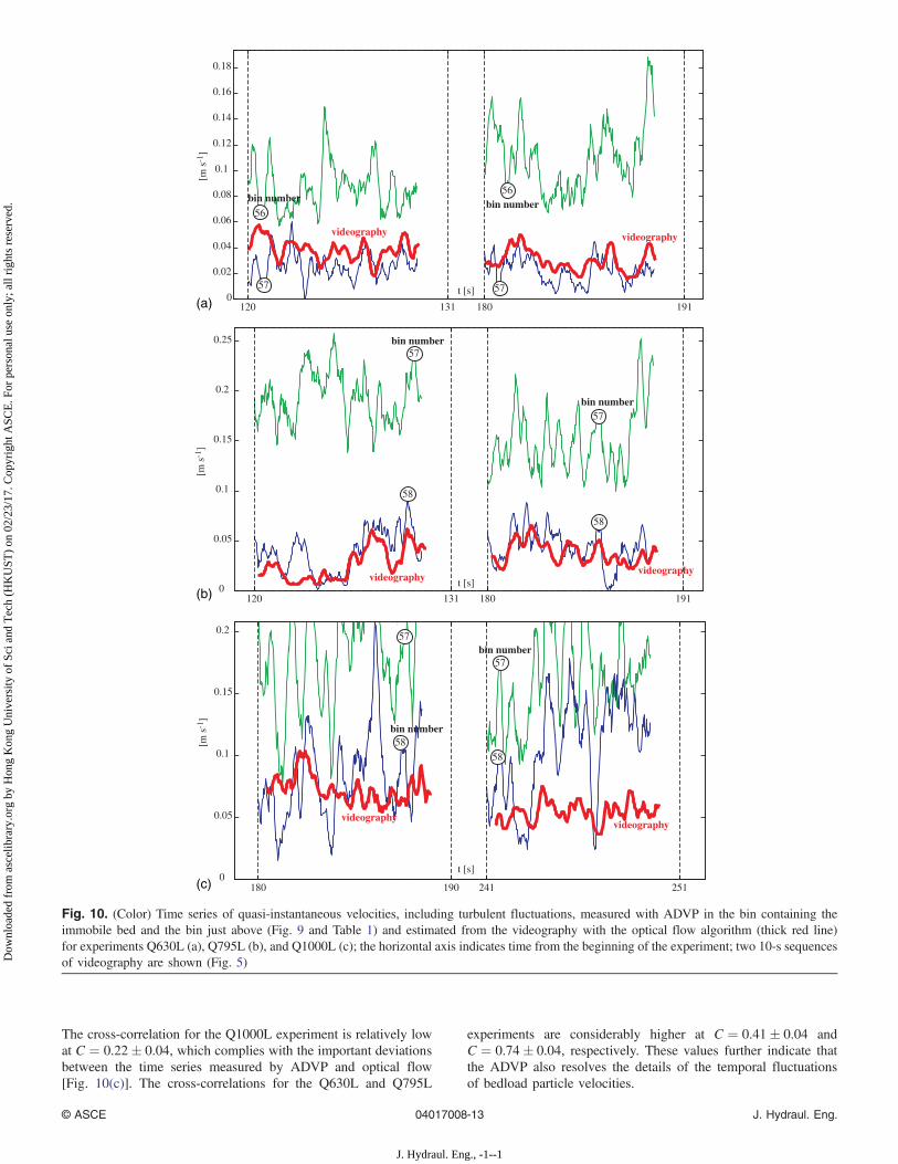
The cross-correlation for the Q1000L experiment is relatively lowat C ¼ 0.22� 0.04, which complies with the important deviationsbetween the time series measured by ADVP and optical flow[Fig. 10(c)]. The cross-correlations for the Q630L and Q795L

experiments are considerably higher at C ¼ 0.41� 0.04 andC ¼ 0.74� 0.04, respectively. These values further indicate thatthe ADVP also resolves the details of the temporal fluctuationsof bedload particle velocities.

180 190 241 251 0

0.05

0.1

0.15

0.2

[m s

-1]

t [s]

[m s

-1]

t [s]

[m s

-1]

t [s]

120 131 180 191 0

0.05

0.1

0.15

0.2

0.25

120 131 180 191 0

0.02

0.04

0.06

0.08

0.1

0.12

0.14

0.16

0.18

bin number

57

bin number56

57

bin number57

58

bin number57

58

bin number

57

58

bin number57

58

56

videography videography

videographyvideography

videographyvideography

(a)

(b)

(c)

Fig. 10. (Color) Time series of quasi-instantaneous velocities, including turbulent fluctuations, measured with ADVP in the bin containing theimmobile bed and the bin just above (Fig. 9 and Table 1) and estimated from the videography with the optical flow algorithm (thick red line)for experiments Q630L (a), Q795L (b), and Q1000L (c); the horizontal axis indicates time from the beginning of the experiment; two 10-s sequencesof videography are shown (Fig. 5)



Dow

nloa

ded

from

asc

elib

rary

.org

by

Hon

g K

ong

Uni

vers

ity o

f Sc

i and

Tec

h (H

KU

ST)

on 0

2/23

/17.

Cop

yrig

ht A

SCE

. For

per

sona

l use

onl

y; a

ll ri

ghts

res

erve

d.

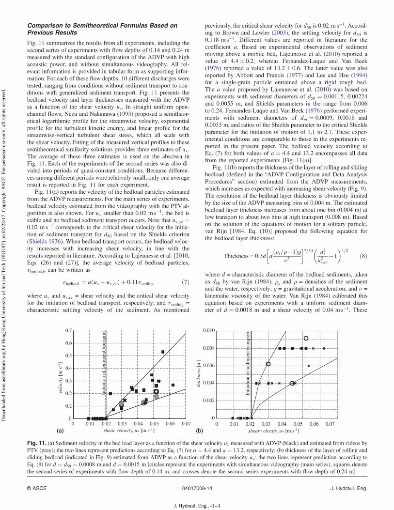
Comparison to Semitheoretical Formulas Based onPrevious Results

Fig. 11 summarizes the results from all experiments, including thesecond series of experiments with flow depths of 0.14 and 0.24 mmeasured with the standard configuration of the ADVP with highacoustic power, and without simultaneous videography. All rel-evant information is provided in tabular form as supporting infor-mation. For each of these flow depths, 10 different discharges weretested, ranging from conditions without sediment transport to con-ditions with generalized sediment transport. Fig. 11 presents thebedload velocity and layer thicknesses measured with the ADVPas a function of the shear velocity u�. In straight uniform open-channel flows, Nezu and Nakagawa (1993) proposed a semitheor-etical logarithmic profile for the streamwise velocity, exponentialprofile for the turbulent kinetic energy, and linear profile for thestreamwise-vertical turbulent shear stress, which all scale withthe shear velocity. Fitting of the measured vertical profiles to thesesemitheoretical similarity solutions provides three estimates of u�.The average of these three estimates is used on the abscissa inFig. 11. Each of the experiments of the second series was also di-vided into periods of quasi-constant conditions. Because differen-ces among different periods were relatively small, only one averageresult is reported in Fig. 11 for each experiment.

Fig. 11(a) reports the velocity of the bedload particles estimatedfrom the ADVP measurements. For the main series of experiments,bedload velocity estimated from the videography with the PTV al-gorithm is also shown. For u� smaller than 0.02 ms−1, the bed isstable and no bedload sediment transport occurs. Note that u�;cr ¼0.02 ms−1 corresponds to the critical shear velocity for the initia-tion of sediment transport for d50 based on the Shields criterion(Shields 1936). When bedload transport occurs, the bedload veloc-ity increases with increasing shear velocity, in line with theresults reported in literature. According to Lajeunesse et al. [2010,Eqs. (26) and (27)], the average velocity of bedload particles,vbedload, can be written as

vbedload ¼ aðu� − u�;crÞ þ 0.11vsettling ð7Þ

where u� and u�;cr = shear velocity and the critical shear velocityfor the initiation of bedload transport, respectively; and vsettling =characteristic settling velocity of the sediment. As mentioned

previously, the critical shear velocity for d50 is 0.02 ms−1. Accord-ing to Brown and Lawler (2003), the settling velocity for d50 is0.118 ms−1. Different values are reported in literature for thecoefficient a. Based on experimental observations of sedimentmoving above a mobile bed, Lajeunesse et al. (2010) reported avalue of 4.4� 0.2, whereas Fernandez-Luque and Van Beek(1976) reported a value of 13.2� 0.6. The latter value was alsoreported by Abbott and Francis (1977) and Lee and Hsu (1994)for a single-grain particle entrained above a rigid rough bed.The a value proposed by Lajeunesse et al. (2010) was based onexperiments with sediment diameters of d50 ¼ 0.00115, 0.00224and 0.0055 m, and Shields parameters in the range from 0.006to 0.24. Fernandez-Luque and Van Beek (1976) performed experi-ments with sediment diameters of dm ¼ 0.0009, 0.0018 and0.0033 m, and ratios of the Shields parameter to the critical Shieldsparameter for the initiation of motion of 1.1 to 2.7. These exper-imental conditions are comparable to those in the experiments re-ported in the present paper. The bedload velocity according toEq. (7) for both values of a ¼ 4.4 and 13.2 encompasses all datafrom the reported experiments [Fig. 11(a)].

Fig. 11(b) reports the thickness of the layer of rolling and slidingbedload (defined in the “ADVP Configuration and Data AnalysisProcedures” section) estimated from the ADVP measurements,which increases as expected with increasing shear velocity (Fig. 9).The resolution of the bedload layer thickness is obviously limitedby the size of the ADVP measuring bins of 0.004 m. The estimatedbedload layer thickness increases from about one bin (0.004 m) atlow transport to about two bins at high transport (0.008 m). Basedon the solution of the equations of motion for a solitary particle,van Rijn [1984, Eq. (10)] proposed the following equation forthe bedload layer thickness:

Thickness¼0.3d

�dðρs=ρ−1Þg

ν2

�7=30

�u2�u2�;cr

−1

�1=2

ð8Þ

where d = characteristic diameter of the bedload sediments, takenas d50 by van Rijn (1984); ρs and ρ = densities of the sedimentand the water, respectively; g = gravitational acceleration; and ν =kinematic viscosity of the water. Van Rijn (1984) calibrated thisequation based on experiments with a uniform sediment diam-eter of d ¼ 0.0018 m and a shear velocity of 0.04 ms−1. These

0 0.01 0.02 0.03 0.04 0.05 0.06 0.070

0.2

0.2

0.3

0.4

0.5

0.6

0.7

velo

city

[m

s-1

]

shear velocity, u* [m s-1]

Initi

atio

n of

sed

imen

t tra

nspo

rt

0 0.01 0.02 0.03 0.04 0.05 0.06 0.070

0.002

0.004

0.006

0.008

0.010

thic

knes

s [m

]

shear velocity, u* [m s-1]

Initi

atio

n of

sed

imen

t tra

nspo

rt

(a) (b)

Fig. 11. (a) Sediment velocity in the bed load layer as a function of the shear velocity u� measured with ADVP (black) and estimated from videos byPTV (gray); the two lines represent predictions according to Eq. (7) for a ¼ 4.4 and a ¼ 13.2, respectively; (b) thickness of the layer of rolling andsliding bedload (indicated in Fig. 9) estimated from ADVP as a function of the shear velocity u�; the two lines represent prediction according toEq. (8) for d ¼ d50 ¼ 0.0008 m and d ¼ 0.0015 m [circles represent the experiments with simultaneous videography (main series), squares denotethe second series of experiments with flow depth of 0.14 m, and crosses denote the second series experiments with flow depth of 0.24 m]



Dow

nloa

ded

from

asc

elib

rary

.org

by

Hon

g K

ong

Uni

vers

ity o

f Sc

i and

Tec

h (H

KU

ST)

on 0

2/23

/17.

Cop

yrig

ht A

SCE

. For

per

sona

l use

onl

y; a

ll ri

ghts

res

erve

d.

parameters are in the same range as in the experiments reported inthis study. All data on the bedload layer thickness estimated fromthe ADVP measurements in the present experiments are con-strained by two curves, corresponding to predictions based onEq. (8) for bedload sediment diameters of d ¼ d50 ¼ 0.0008 m andd ¼ 0.0015 m. Hence, the ADVP estimates of the bedload layerthickness comply with the equation and underlying experimentsof van Rijn (1984).

Results for the velocities and thicknesses are quite similar forexperiments Q630 and Q795 in the main series of experiments,and strongly increase from Q795 to Q1000. This behavior can beattributed to the gradual formation of the armor layer in Q630,which limits bedload transport in Q795, and the breakup of thearmor layer in Q1000.

Comparison of Standard ADVP Configuration andADVP Configuration Optimized for BedloadMeasurements

For both the sediment velocity in the bedload layer, and thethickness of the dominant bedload layer, results of the experimentswith a flow depth of 0.24 m in the second series with standardADVP configuration (Table S2 of the supporting information)agree well with the results in the main series with ADVP configu-ration optimized for bedload measurements (Table 2). Experimentswith similar hydraulic conditions are compared (Q630L versusQ605H, Q795L versus Q794H and Q795H, and Q1000L versusQ897H). The relative and absolute differences between the averageparticle velocity estimated with standard and optimized ADVP con-figurations are 20� 8% and 0.032� 0.025 ms−1, respectively.This absolute difference is much smaller than the velocity variationwithin one bin (Fig. 9). Both ADVP configurations provided iden-tical estimations of the thickness of the dominant bedload layer.This confirms that the standard ADVP configuration provides re-liable estimations of the bedload characteristics.

Discussion and Conclusions

Previous experiments have indicated that near-bed velocities candeviate from the logarithmic profile as a result of beam geometryeffects [i.e., contamination of the near-bed bins by high-intensityscatter from the immobile bed (Hay et al. 2012a, b, c)], and asa result of the presence of bedload sediment transport (Naqshbandet al. 2014b). The ellipses of equal acoustic travel time for thenear-bed bins are illustrated in Figs. 1(a and b) for the ADVP con-figurations adopted in the reported experiments. These purely geo-metrical considerations indicate a potential contamination zone as aresult of beam geometry effects of approximately 0.01 m. This is aconservative estimation, however, which does not take into accountthat the acoustic power is maximal in the center of the insonifiedbeam and decays in a Gaussian way toward its edges. In all experi-ments without sediment transport reported in this paper, the ADVPresolved the law of the wall logarithmic velocity profile, includingin the first bin above the immobile bed [Fig. 3(a)]. This indicatesthat the contamination zone caused by beam geometry effects issmaller than 0.004 m. In contrast, in all experiments with bedloadsediment transport reported in this paper, velocities in the near-bed region where bedload sediment transport occurs were system-atically smaller than expected from the logarithmic law of thewall [Figs. 3(a and b) and 9], similar to observations by Naqshbandet al. (2014b). The deviating velocities occurred in a layer of ap-proximately 0.004 to 0.02 m from the immobile bed (Figs. 3 and 9).These observations indicate that the velocity deficit in the near-bed

region is essentially related to the transport of bedload in the re-ported experiments.

Results from all three strategies corroborate the main hypothesisof the present paper, that the ADVP does measure sediment veloc-ities also in the near-bed layer where bedload transport occurs.First, the backscattered raw return signals IðtÞ recorded by theADVP’s receivers reveal a clear footprint of the bedload sedimentparticles. The magnitude of IðtÞ in the bins where bedload sedimenttransport occurs clearly exceeds that of bins above in the clear waterflow (Figs. 2 and 6), which is because of the fact that sedimentparticles backscatter considerably more acoustic energy than microair bubbles in the clear water (Hurther et al. 2011). Thus, the sedi-ment particles are the main scattering sources in the insonifiedwater column; therefore, it is their velocity that is measured bythe ADVP. Spectra of the IðtÞ signals are near-Gaussian in the clearwater and left-skewed near the bed where bedload sediment trans-port occurs. The latter distribution is characteristic for bedload sedi-ment transport (Fig. 7), in agreement with recent findings (Drakeet al. 1988, Rennie and Millar 2007, Lajeunesse et al. 2010, Furbishet al. 2012). Second, results from the simultaneous videography ofthe bedload sediment transport are in good agreement with ADVPresults. Time-averaged velocities measured with the ADVP in thelayer of rolling and sliding bedload transport agree well with thoseestimated from the digital video images of the moving sedimentwith a particle tracking algorithm (Fig. 9). Moreover, velocity timeseries (mean and fluctuating components) measured with theADVP in the bin containing the immobile-bed surface agree wellwith the time series of the average bed velocity estimated with theoptical flow algorithm (Fig. 10). Third, ADVP-based estimates ofthe bedload velocities and thickness of the bedload layer are inagreement with semitheoretical formulas based on previous experi-ments proposed by Lajeunesse et al. (2010) and van Rijn (1984),respectively, for a broad range of hydraulic conditions (Fig. 11).

The ADVP configuration optimized for bedload measurementsonly marginally performs better than the standard configuration forflow measurements, which also provides satisfactory estimates ofthe sediment velocity and transport layer thickness.

These findings corroborate the hypothesis of Hurther et al.(2011) and Naqshband et al. (2014b) that the ADVP can measurethe time-averaged velocity of bedload particles, and the hypothesisof Naqshband et al. (2014a) that also measures the temporal fluc-tuations of the particle velocities. The shear velocities in the re-ported experiments were comparable to those in the experimentsof Naqshband et al. (2014a, b), but their sediment size was approx-imately 10 times smaller, leading to Shields numbers that were ap-proximately 10 times higher, and resulting in more intense bedloadtransport and significant suspended load transport. Both the presentstudy and Naqshband et al. (2014a, b) used a similar ADVP withcarrier frequency f0 ¼ 1 MHz, resulting in a wavelength of theemitted acoustic pulses of approximately λ ¼ c=f0 ¼ 0.0015 m.The sediment particles were smaller than this wavelength inNaqshband’s experiment, leading to Rayleigh backscattering of theacoustic pulse. The particles were larger than this wavelength in ourexperiments, leading to geometric scattering. These results indicatethat the ADVP is able to measure turbulent bedload velocities andthe bedload layer thickness for a broad range of sediment diametersand different regimes of scattering.

These results confirm that ACVPs (Hurther et al. 2011), whichintegrate an ADVP with an ABS, are able to measure turbulentsediment fluxes according to Eq. (1). The ability of ABS to mea-sure sediment concentration in the entire water column, includingthe bedload layer, has been demonstrated (Naqshband et al. 2014b).When sediment transport occurs, the ADVP provides unbiasedmeasurements of the sediment velocity us, even in the near-bed



Dow

nloa

ded

from

asc

elib

rary

.org

by

Hon

g K

ong

Uni

vers

ity o

f Sc

i and

Tec

h (H

KU

ST)

on 0

2/23

/17.

Cop

yrig

ht A

SCE

. For

per

sona

l use

onl

y; a

ll ri

ghts

res

erve

d.


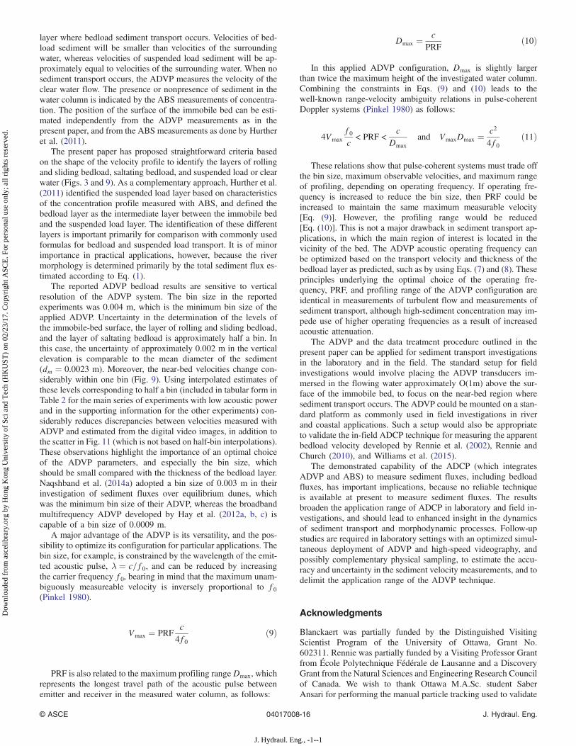
layer where bedload sediment transport occurs. Velocities of bed-load sediment will be smaller than velocities of the surroundingwater, whereas velocities of suspended load sediment will be ap-proximately equal to velocities of the surrounding water. When nosediment transport occurs, the ADVP measures the velocity of theclear water flow. The presence or nonpresence of sediment in thewater column is indicated by the ABS measurements of concentra-tion. The position of the surface of the immobile bed can be esti-mated independently from the ADVP measurements as in thepresent paper, and from the ABS measurements as done by Hurtheret al. (2011).

The present paper has proposed straightforward criteria basedon the shape of the velocity profile to identify the layers of rollingand sliding bedload, saltating bedload, and suspended load or clearwater (Figs. 3 and 9). As a complementary approach, Hurther et al.(2011) identified the suspended load layer based on characteristicsof the concentration profile measured with ABS, and defined thebedload layer as the intermediate layer between the immobile bedand the suspended load layer. The identification of these differentlayers is important primarily for comparison with commonly usedformulas for bedload and suspended load transport. It is of minorimportance in practical applications, however, because the rivermorphology is determined primarily by the total sediment flux es-timated according to Eq. (1).

The reported ADVP bedload results are sensitive to verticalresolution of the ADVP system. The bin size in the reportedexperiments was 0.004 m, which is the minimum bin size of theapplied ADVP. Uncertainty in the determination of the levels ofthe immobile-bed surface, the layer of rolling and sliding bedload,and the layer of saltating bedload is approximately half a bin. Inthis case, the uncertainty of approximately 0.002 m in the verticalelevation is comparable to the mean diameter of the sediment(dm ¼ 0.0023 m). Moreover, the near-bed velocities change con-siderably within one bin (Fig. 9). Using interpolated estimates ofthese levels corresponding to half a bin (included in tabular form inTable 2 for the main series of experiments with low acoustic powerand in the supporting information for the other experiments) con-siderably reduces discrepancies between velocities measured withADVP and estimated from the digital video images, in addition tothe scatter in Fig. 11 (which is not based on half-bin interpolations).These observations highlight the importance of an optimal choiceof the ADVP parameters, and especially the bin size, whichshould be small compared with the thickness of the bedload layer.Naqshband et al. (2014a) adopted a bin size of 0.003 m in theirinvestigation of sediment fluxes over equilibrium dunes, whichwas the minimum bin size of their ADVP, whereas the broadbandmultifrequency ADVP developed by Hay et al. (2012a, b, c) iscapable of a bin size of 0.0009 m.

A major advantage of the ADVP is its versatility, and the pos-sibility to optimize its configuration for particular applications. Thebin size, for example, is constrained by the wavelength of the emit-ted acoustic pulse, λ ¼ c=f0, and can be reduced by increasingthe carrier frequency f0, bearing in mind that the maximum unam-biguously measureable velocity is inversely proportional to f0(Pinkel 1980).

Vmax ¼ PRFc4f0

ð9Þ

PRF is also related to the maximum profiling rangeDmax, whichrepresents the longest travel path of the acoustic pulse betweenemitter and receiver in the measured water column, as follows:

Dmax ¼c

PRFð10Þ

In this applied ADVP configuration, Dmax is slightly largerthan twice the maximum height of the investigated water column.Combining the constraints in Eqs. (9) and (10) leads to thewell-known range-velocity ambiguity relations in pulse-coherentDoppler systems (Pinkel 1980) as follows:

4Vmaxf0c

< PRF <c

Dmaxand VmaxDmax ¼

c2

4f0ð11Þ

These relations show that pulse-coherent systems must trade offthe bin size, maximum observable velocities, and maximum rangeof profiling, depending on operating frequency. If operating fre-quency is increased to reduce the bin size, then PRF could beincreased to maintain the same maximum measurable velocity[Eq. (9)]. However, the profiling range would be reduced[Eq. (10)]. This is not a major drawback in sediment transport ap-plications, in which the main region of interest is located in thevicinity of the bed. The ADVP acoustic operating frequency canbe optimized based on the transport velocity and thickness of thebedload layer as predicted, such as by using Eqs. (7) and (8). Theseprinciples underlying the optimal choice of the operating fre-quency, PRF, and profiling range of the ADVP configuration areidentical in measurements of turbulent flow and measurements ofsediment transport, although high-sediment concentration may im-pede use of higher operating frequencies as a result of increasedacoustic attenuation.

The ADVP and the data treatment procedure outlined in thepresent paper can be applied for sediment transport investigationsin the laboratory and in the field. The standard setup for fieldinvestigations would involve placing the ADVP transducers im-mersed in the flowing water approximately O(1m) above the sur-face of the immobile bed, to focus on the near-bed region wheresediment transport occurs. The ADVP could be mounted on a stan-dard platform as commonly used in field investigations in riverand coastal applications. Such a setup would also be appropriateto validate the in-field ADCP technique for measuring the apparentbedload velocity developed by Rennie et al. (2002), Rennie andChurch (2010), and Williams et al. (2015).

The demonstrated capability of the ADCP (which integratesADVP and ABS) to measure sediment fluxes, including bedloadfluxes, has important implications, because no reliable techniqueis available at present to measure sediment fluxes. The resultsbroaden the application range of ADCP in laboratory and field in-vestigations, and should lead to enhanced insight in the dynamicsof sediment transport and morphodynamic processes. Follow-upstudies are required in laboratory settings with an optimized simul-taneous deployment of ADVP and high-speed videography, andpossibly complementary physical sampling, to estimate the accu-racy and uncertainty in the sediment velocity measurements, and todelimit the application range of the ADVP technique.

Acknowledgments

Blanckaert was partially funded by the Distinguished VisitingScientist Program of the University of Ottawa, Grant No.602311. Rennie was partially funded by a Visiting Professor Grantfrom École Polytechnique Fédérale de Lausanne and a DiscoveryGrant from the Natural Sciences and Engineering Research Councilof Canada. We wish to thank Ottawa M.A.Sc. student SaberAnsari for performing the manual particle tracking used to validate



Dow

nloa

ded

from

asc

elib

rary

.org

by

Hon

g K

ong

Uni

vers

ity o

f Sc

i and

Tec

h (H

KU

ST)

on 0

2/23

/17.

Cop

yrig

ht A

SCE

. For

per

sona

l use

onl

y; a

ll ri

ghts

res

erve

d.

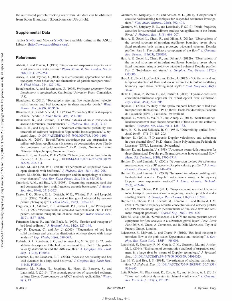
the automated particle tracking algorithm. All data can be obtainedfrom Koen Blanckaert ([email protected]).

Supplemental Data

Tables S1–S3 and Movies S1–S3 are available online in the ASCELibrary (http://www.ascelibrary.org).

References

Abbott, J., and Francis, J. (1977). “Saltation and suspension trajectories ofsolid grains in a water stream.” Philos. Trans. R. Soc. London, Ser. A,284(1321), 225–254.

Ancey, C., and Heyman, J. (2014). “Amicrostructural approach to bed loadtransport: Mean behaviour and fluctuations of particle transport rates.”J. Fluid Mech., 744, 129–168.

Beutelspacher, A., and Rosenbaum, U. (1998). Projective geometry: Fromfoundations to applications, Cambridge University Press, Cambridge,U.K.

Blanckaert, K. (2010). “Topographic steering, flow recirculation, velocityredistribution, and bed topography in sharp meander bends.” WaterResour. Res., 46(9), W09506.

Blanckaert, K., and de Vriend, H. J. (2004). “Secondary flow in sharp openchannel bends.” J. Fluid Mech., 498, 353–380.

Blanckaert, K., and Lemmin, U. (2006). “Means of noise reduction inacoustic turbulence measurements.” J. Hydraul. Res., 44(1), 3–17.

Bose, S. K., and Dey, S. (2013). “Sediment entrainment probability andthreshold of sediment suspension: Exponential-based approach.” J. Hy-draul. Eng., 10.1061/(ASCE)HY.1943-7900.0000763, 1099–1106.

Bricault, M. (2006). “Rétrodiffusion acoustique par une suspension enmilieu turbulent: Application à la mesure de concentration pour l’étudedes processes hydrosédimentaires.” Ph.D. thesis, Grenoble InstitutNational Polytechnique, Grenoble, France.

Brown, P. P., and Lawler, D. F. (2003). “Sphere drag and settling velocityrevisited.” J. Environ. Eng., 10.1061/(ASCE)0733-9372(2003)129:3(222), 222–231.

Cellino, M., and Graf, W. H. (2000). “Experiments on suspension flow inopen channels with bedforms.” J. Hydraul. Res., 38(4), 289–298.

Church, M. (2006). “Bed material transport and the morphology of alluvialriver channels.” Ann. Rev. Earth Planet. Sci., 34(1), 325–354.

Crawford, A. M., and Hay, A. E. (1993). “Determining suspended sand sizeand concentration from multifrequency acoustic backscatter.” J. Acoust.Soc. Am., 94(6), 3312–3324.

Drake, T. G., Shreve, R. L., Dietrich, W. E., Whiting, P. J., and Leopold,L. B. (1988). “Bedload transport of fine gravel observed by motion-picture photography.” J. Fluid Mech., 192(1), 193–217.

Ferguson, R. I., Ashmore, P. E., Ashworth, P. J., Paola, C., and Prestegaard,K. L. (1992). “Measurements in a braided river chute and lobe. 1: Flowpattern, sediment transport, and channel change.” Water Resour. Res.,28(7), 1877–1886.

Fernandez-Luque, R., and Van Beek, R. (1976). “Erosion and transport ofbed-load sediment.” J. Hydraul. Res., 14(2), 127–144.

Frey, P., Ducottet, C., and Jay, J. (2003). “Fluctuations of bed loadsolid discharge and grain size distribution on steep slopes with imageanalysis.” Exp. Fluids, 35(6), 589–597.

Furbish, D. J., Roseberry, J. C., and Schmeeckle, M. W. (2012). “A prob-abilistic description of the bed load sediment flux. Part 3: The particlevelocity distribution and the diffusive flux.” J. Geophys. Res. EarthSurf., 117(3), F03033.

Gaeuman, D., and Jacobson, R. B. (2006). “Acoustic bed velocity and bedload dynamics in a large sand bed river.” J. Geophys. Res. Earth Surf.,111(2), F02005.

Guerrero, M., Rüther, N., Szupiany, R., Haun, S., Baranya, S., andLatosinski, F. (2016). “The acoustic properties of suspended sedimentin large Rivers: Consequences on ADCP methods applicability.”Water,8(1), 13.

Guerrero, M., Szupiany, R. N., and Amsler, M. L. (2011). “Comparison ofacoustic backscattering techniques for suspended sediments investiga-tions.” Flow Meas. Instrum., 22(5), 392–401.

Guerrero, M., Szupiany, R. N., and Latosinski, F. (2013). “Multi-frequencyacoustics for suspended sediment studies: An application in the ParanaRiver.” J. Hydraul. Res., 51(6), 696–707.

Hay, A. E., Zedel, L., Cheel, R., and Dillon, J. (2012a). “Observations ofthe vertical structure of turbulent oscillatory boundary layers abovefixed roughness beds using a prototype wideband coherent Dopplerprofiler. Part 1: The oscillatory component of the flow.” J. Geophys.Res. Oceans, 117(C3), C03005.

Hay, A. E., Zedel, L., Cheel, R., and Dillon, J. (2012b). “Observations ofthe vertical structure of turbulent oscillatory boundary layers abovefixed roughness using a prototype wideband coherent Doppler profiler.Part 2: Turbulence and stress.” J. Geophys. Res. Oceans, 117(3),C03006.

Hay, A. E., Zedel, L., Cheel, R., and Dillon, J. (2012c). “On the vertical andtemporal structure of flow and stress within the turbulent oscillatoryboundary layer above evolving sand ripples.” Cont. Shelf Res., 46(1),31–49.

Heitz, D., Héas, P., Mémin, E., and, Carlier, J. (2008). “Dynamic consistentcorrelation-variational approach for robust optical flow estimation.”Exp. Fluids, 45(4), 595–608.

Heyman, J. (2014). “A study of the spatio-temporal behaviour of bed loadtransport rate fluctuations.” Ph.D. thesis, École Polytechnique Fédéralede Lausanne (EPFL), Lausanne, Switzerland.

Heyman, J., Mettra, F., Ma, H. B., and Ancey, C. (2013). “Statistics of bed-load transport over steep slopes: Separation of time scales and collectivemotion.” Geophys. Res. Lett., 40(1), 128–133.

Horn, B. K. P., and Schunck, B. G. (1981). “Determining optical flow.”Artif. Intell., 17(1–3), 185–203.

Hurther, D. (2001). “3-D acoustic Doppler velocimetry and turbulencein open-channel flow.” Ph.D. thesis, École Polytechnique Fédérale deLausanne (EPFL), Lausanne, Switzerland.

Hurther, D., and Lemmin, U. (1998). “A constant beamwidth transducer forthree-dimensional Doppler profile measurements in open channel flow.”Meas. Sci. Technol., 9(10), 1706–1714.

Hurther, D., and Lemmin, U. (2001). “A correction method for turbulencemeasurements with a 3D acoustic Doppler velocity profiler.” J. Atmos.Oceanic. Technol., 18(3), 446–458.

Hurther, D., and Lemmin, U. (2008). “Improved turbulence profiling withfield-adapted acoustic Doppler velocimeters using a bifrequencyDoppler noise suppression method.” J. Atmos. Oceanic. Technol.,25(3), 452–463.

Hurther, D., and Thorne, P. D. (2011). “Suspension and near-bed load sedi-ment transport processes above a migrating, sand-rippled bed undershoaling waves.” J. Geophys. Res. Oceans, 116(C7), C07001.

Hurther, D., Thorne, P. D., Bricault, M., Lemmin, U., and Barnoud, J. M.(2011). “A multi-frequency acoustic concentration and velocity profiler(ACVP) for boundary layer measurements of fine-scale flow and sedi-ment transport processes.” Coastal Eng., 58(7), 594–605.

Klar, M., et al. (2004). “Simultaneous 3-D PTV and micro-pressure sensorequipment for flow analysis in a subsurface gravel layer.” Proc. RiverFlow 2004, M. Greco, A. Carravetta, and R. Della Morte, eds., Taylor &Francis Group, London.

Lajeunesse, E., Malverti, L., and Charru, F. (2010). “Bed load transport inturbulent flow at the grain scale: Experiments and modeling.” J. Geo-phys. Res. Earth Surf., 115(F4), F04001.

Latosinski, F., Szupiany, R. N., García, C. M., Guerrero, M., and Amsler,M. L. (2014). “Estimation of concentration and load of suspended sedi-ment in a large river by means of Doppler technology.” J. Hydraul.Eng., 10.1061/(ASCE)HY.1943-7900.0000859, 04014023.

Lee, H. Y., and Hsu, I. S. (1994). “Investigation of saltating particle mo-tions.” J. Hydraul. Eng., 10.1061/(ASCE)0733-9429(1994)120:7(831),831–845.

Leite Ribeiro, M., Blanckaert, K., Roy, A. G., and Schleiss, A. J. (2012).“Flow and sediment dynamics in channel confluences.” J. Geophys.Res. Earth Surf., 117(1), F01035.



Dow

nloa

ded

from

asc

elib

rary

.org

by

Hon

g K

ong

Uni

vers

ity o

f Sc

i and

Tec

h (H

KU

ST)

on 0

2/23

/17.

Cop

yrig

ht A

SCE

. For

per

sona

l use

onl

y; a

ll ri

ghts

res

erve

d.






http://www.ascelibrary.org

https://doi.org/10.1098/rsta.1977.0009

https://doi.org/10.1098/rsta.1977.0009

https://doi.org/10.1017/jfm.2014.74

https://doi.org/10.1029/2009WR008303

https://doi.org/10.1029/2009WR008303

https://doi.org/10.1017/S0022112003006979

https://doi.org/10.1080/00221686.2006.9521657


https://doi.org/10.1061/(ASCE)0733-9372(2003)129:3(222)


https://doi.org/10.1080/00221680009498328

https://doi.org/10.1146/annurev.earth.33.092203.122721

https://doi.org/10.1121/1.407237

https://doi.org/10.1121/1.407237

https://doi.org/10.1017/S0022112088001831

https://doi.org/10.1029/92WR00700

https://doi.org/10.1029/92WR00700

https://doi.org/10.1080/00221687609499677

https://doi.org/10.1007/s00348-003-0707-9

https://doi.org/10.1029/2012JF002355

https://doi.org/10.1029/2012JF002355

https://doi.org/10.1029/2005JF000411

https://doi.org/10.1029/2005JF000411

https://doi.org/10.3390/w8010013

https://doi.org/10.3390/w8010013

https://doi.org/10.1016/j.flowmeasinst.2011.06.003

https://doi.org/10.1080/00221686.2013.849296

https://doi.org/10.1029/2011JC007114

https://doi.org/10.1029/2011JC007114

https://doi.org/10.1029/2011JC007113

https://doi.org/10.1029/2011JC007113

https://doi.org/10.1016/j.csr.2012.02.009


https://doi.org/10.1007/s00348-008-0567-4

https://doi.org/10.1029/2012GL054280

https://doi.org/10.1088/0957-0233/9/10/010

https://doi.org/10.1175/1520-0426(2001)018<0446:ACMFTMtpmkset

https://doi.org/10.1175/1520-0426(2001)018<0446:ACMFTMtpmkset

https://doi.org/10.1029/2010JC006774

https://doi.org/10.1016/j.coastaleng.2011.01.006

https://doi.org/10.1029/2009JF001628

https://doi.org/10.1029/2009JF001628




https://doi.org/10.1029/2011JF002171

https://doi.org/10.1029/2011JF002171

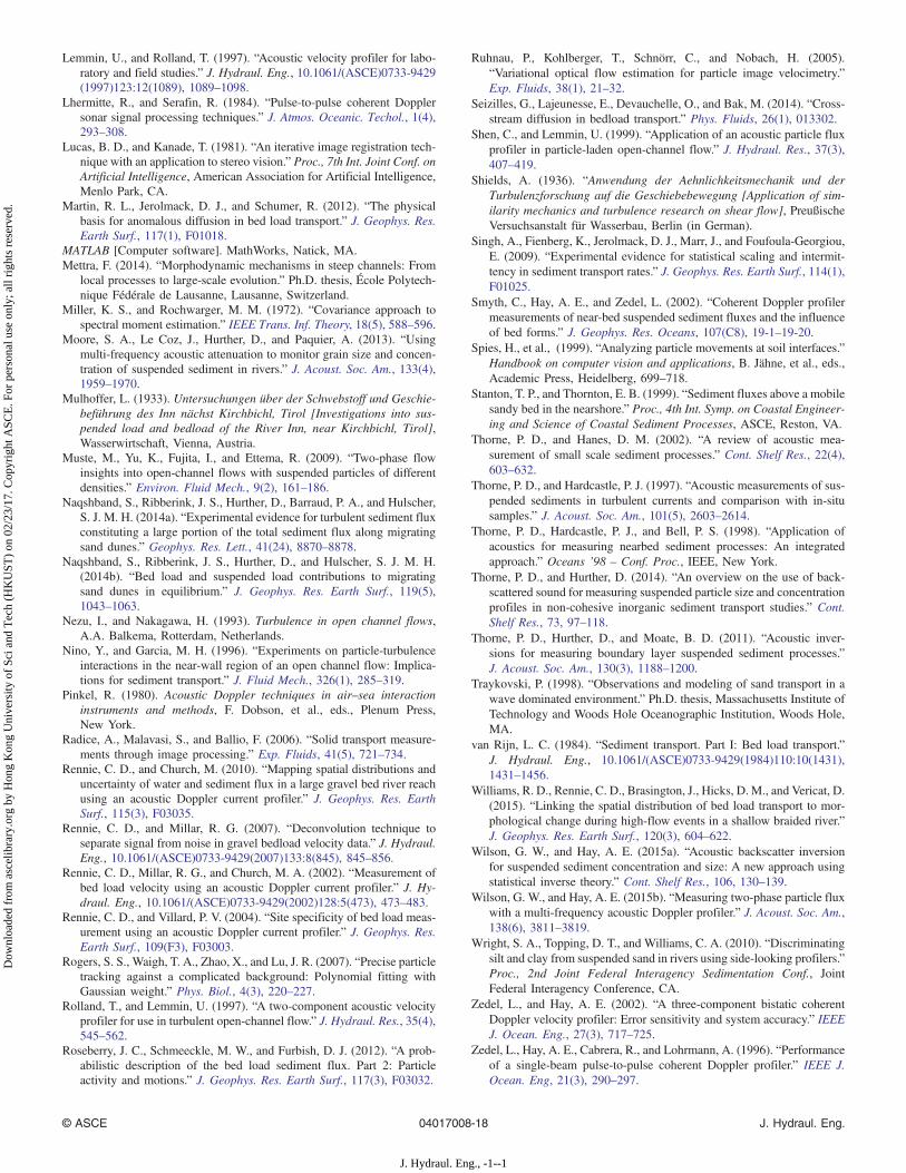
Lemmin, U., and Rolland, T. (1997). “Acoustic velocity profiler for labo-ratory and field studies.” J. Hydraul. Eng., 10.1061/(ASCE)0733-9429(1997)123:12(1089), 1089–1098.

Lhermitte, R., and Serafin, R. (1984). “Pulse-to-pulse coherent Dopplersonar signal processing techniques.” J. Atmos. Oceanic. Techol., 1(4),293–308.

Lucas, B. D., and Kanade, T. (1981). “An iterative image registration tech-nique with an application to stereo vision.” Proc., 7th Int. Joint Conf. onArtificial Intelligence, American Association for Artificial Intelligence,Menlo Park, CA.

Martin, R. L., Jerolmack, D. J., and Schumer, R. (2012). “The physicalbasis for anomalous diffusion in bed load transport.” J. Geophys. Res.Earth Surf., 117(1), F01018.

MATLAB [Computer software]. MathWorks, Natick, MA.Mettra, F. (2014). “Morphodynamic mechanisms in steep channels: From

local processes to large-scale evolution.” Ph.D. thesis, École Polytech-nique Fédérale de Lausanne, Lausanne, Switzerland.

Miller, K. S., and Rochwarger, M. M. (1972). “Covariance approach tospectral moment estimation.” IEEE Trans. Inf. Theory, 18(5), 588–596.

Moore, S. A., Le Coz, J., Hurther, D., and Paquier, A. (2013). “Usingmulti-frequency acoustic attenuation to monitor grain size and concen-tration of suspended sediment in rivers.” J. Acoust. Soc. Am., 133(4),1959–1970.

Mulhoffer, L. (1933). Untersuchungen über der Schwebstoff und Geschie-beführung des Inn nächst Kirchbichl, Tirol [Investigations into sus-pended load and bedload of the River Inn, near Kirchbichl, Tirol],Wasserwirtschaft, Vienna, Austria.

Muste, M., Yu, K., Fujita, I., and Ettema, R. (2009). “Two-phase flowinsights into open-channel flows with suspended particles of differentdensities.” Environ. Fluid Mech., 9(2), 161–186.

Naqshband, S., Ribberink, J. S., Hurther, D., Barraud, P. A., and Hulscher,S. J. M. H. (2014a). “Experimental evidence for turbulent sediment fluxconstituting a large portion of the total sediment flux along migratingsand dunes.” Geophys. Res. Lett., 41(24), 8870–8878.

Naqshband, S., Ribberink, J. S., Hurther, D., and Hulscher, S. J. M. H.(2014b). “Bed load and suspended load contributions to migratingsand dunes in equilibrium.” J. Geophys. Res. Earth Surf., 119(5),1043–1063.

Nezu, I., and Nakagawa, H. (1993). Turbulence in open channel flows,A.A. Balkema, Rotterdam, Netherlands.

Nino, Y., and Garcia, M. H. (1996). “Experiments on particle-turbulenceinteractions in the near-wall region of an open channel flow: Implica-tions for sediment transport.” J. Fluid Mech., 326(1), 285–319.

Pinkel, R. (1980). Acoustic Doppler techniques in air–sea interactioninstruments and methods, F. Dobson, et al., eds., Plenum Press,New York.

Radice, A., Malavasi, S., and Ballio, F. (2006). “Solid transport measure-ments through image processing.” Exp. Fluids, 41(5), 721–734.

Rennie, C. D., and Church, M. (2010). “Mapping spatial distributions anduncertainty of water and sediment flux in a large gravel bed river reachusing an acoustic Doppler current profiler.” J. Geophys. Res. EarthSurf., 115(3), F03035.

Rennie, C. D., and Millar, R. G. (2007). “Deconvolution technique toseparate signal from noise in gravel bedload velocity data.” J. Hydraul.Eng., 10.1061/(ASCE)0733-9429(2007)133:8(845), 845–856.

Rennie, C. D., Millar, R. G., and Church, M. A. (2002). “Measurement ofbed load velocity using an acoustic Doppler current profiler.” J. Hy-draul. Eng., 10.1061/(ASCE)0733-9429(2002)128:5(473), 473–483.

Rennie, C. D., and Villard, P. V. (2004). “Site specificity of bed load meas-urement using an acoustic Doppler current profiler.” J. Geophys. Res.Earth Surf., 109(F3), F03003.

Rogers, S. S., Waigh, T. A., Zhao, X., and Lu, J. R. (2007). “Precise particletracking against a complicated background: Polynomial fitting withGaussian weight.” Phys. Biol., 4(3), 220–227.

Rolland, T., and Lemmin, U. (1997). “A two-component acoustic velocityprofiler for use in turbulent open-channel flow.” J. Hydraul. Res., 35(4),545–562.

Roseberry, J. C., Schmeeckle, M. W., and Furbish, D. J. (2012). “A prob-abilistic description of the bed load sediment flux. Part 2: Particleactivity and motions.” J. Geophys. Res. Earth Surf., 117(3), F03032.

Ruhnau, P., Kohlberger, T., Schnörr, C., and Nobach, H. (2005).“Variational optical flow estimation for particle image velocimetry.”Exp. Fluids, 38(1), 21–32.

Seizilles, G., Lajeunesse, E., Devauchelle, O., and Bak, M. (2014). “Cross-stream diffusion in bedload transport.” Phys. Fluids, 26(1), 013302.

Shen, C., and Lemmin, U. (1999). “Application of an acoustic particle fluxprofiler in particle-laden open-channel flow.” J. Hydraul. Res., 37(3),407–419.

Shields, A. (1936). “Anwendung der Aehnlichkeitsmechanik und derTurbulenzforschung auf die Geschiebebewegung [Application of sim-ilarity mechanics and turbulence research on shear flow], PreußischeVersuchsanstalt für Wasserbau, Berlin (in German).

Singh, A., Fienberg, K., Jerolmack, D. J., Marr, J., and Foufoula-Georgiou,E. (2009). “Experimental evidence for statistical scaling and intermit-tency in sediment transport rates.” J. Geophys. Res. Earth Surf., 114(1),F01025.

Smyth, C., Hay, A. E., and Zedel, L. (2002). “Coherent Doppler profilermeasurements of near-bed suspended sediment fluxes and the influenceof bed forms.” J. Geophys. Res. Oceans, 107(C8), 19-1–19-20.

Spies, H., et al., (1999). “Analyzing particle movements at soil interfaces.”Handbook on computer vision and applications, B. Jähne, et al., eds.,Academic Press, Heidelberg, 699–718.

Stanton, T. P., and Thornton, E. B. (1999). “Sediment fluxes above a mobilesandy bed in the nearshore.” Proc., 4th Int. Symp. on Coastal Engineer-ing and Science of Coastal Sediment Processes, ASCE, Reston, VA.

Thorne, P. D., and Hanes, D. M. (2002). “A review of acoustic mea-surement of small scale sediment processes.” Cont. Shelf Res., 22(4),603–632.

Thorne, P. D., and Hardcastle, P. J. (1997). “Acoustic measurements of sus-pended sediments in turbulent currents and comparison with in-situsamples.” J. Acoust. Soc. Am., 101(5), 2603–2614.

Thorne, P. D., Hardcastle, P. J., and Bell, P. S. (1998). “Application ofacoustics for measuring nearbed sediment processes: An integratedapproach.” Oceans ’98 – Conf. Proc., IEEE, New York.

Thorne, P. D., and Hurther, D. (2014). “An overview on the use of back-scattered sound for measuring suspended particle size and concentrationprofiles in non-cohesive inorganic sediment transport studies.” Cont.Shelf Res., 73, 97–118.

Thorne, P. D., Hurther, D., and Moate, B. D. (2011). “Acoustic inver-sions for measuring boundary layer suspended sediment processes.”J. Acoust. Soc. Am., 130(3), 1188–1200.

Traykovski, P. (1998). “Observations and modeling of sand transport in awave dominated environment.” Ph.D. thesis, Massachusetts Institute ofTechnology and Woods Hole Oceanographic Institution, Woods Hole,MA.

van Rijn, L. C. (1984). “Sediment transport. Part I: Bed load transport.”J. Hydraul. Eng., 10.1061/(ASCE)0733-9429(1984)110:10(1431),1431–1456.

Williams, R. D., Rennie, C. D., Brasington, J., Hicks, D. M., and Vericat, D.(2015). “Linking the spatial distribution of bed load transport to mor-phological change during high-flow events in a shallow braided river.”J. Geophys. Res. Earth Surf., 120(3), 604–622.

Wilson, G. W., and Hay, A. E. (2015a). “Acoustic backscatter inversionfor suspended sediment concentration and size: A new approach usingstatistical inverse theory.” Cont. Shelf Res., 106, 130–139.

Wilson, G. W., and Hay, A. E. (2015b). “Measuring two-phase particle fluxwith a multi-frequency acoustic Doppler profiler.” J. Acoust. Soc. Am.,138(6), 3811–3819.

Wright, S. A., Topping, D. T., and Williams, C. A. (2010). “Discriminatingsilt and clay from suspended sand in rivers using side-looking profilers.”Proc., 2nd Joint Federal Interagency Sedimentation Conf., JointFederal Interagency Conference, CA.

Zedel, L., and Hay, A. E. (2002). “A three-component bistatic coherentDoppler velocity profiler: Error sensitivity and system accuracy.” IEEEJ. Ocean. Eng., 27(3), 717–725.

Zedel, L., Hay, A. E., Cabrera, R., and Lohrmann, A. (1996). “Performanceof a single-beam pulse-to-pulse coherent Doppler profiler.” IEEE J.Ocean. Eng, 21(3), 290–297.



Dow

nloa

ded

from

asc

elib

rary

.org

by

Hon

g K

ong

Uni

vers

ity o

f Sc

i and

Tec

h (H

KU

ST)

on 0

2/23

/17.

Cop

yrig

ht A

SCE

. For

per

sona

l use

onl

y; a

ll ri

ghts

res

erve

d.



https://doi.org/10.1175/1520-0426(1984)001<0293:PTPCDStpmkset

https://doi.org/10.1175/1520-0426(1984)001<0293:PTPCDStpmkset

https://doi.org/10.1109/TIT.1972.1054886

https://doi.org/10.1121/1.4792645

https://doi.org/10.1121/1.4792645

https://doi.org/10.1007/s10652-008-9102-7

https://doi.org/10.1002/2014GL062322

https://doi.org/10.1002/2013JF003043

https://doi.org/10.1002/2013JF003043

https://doi.org/10.1017/S0022112096008324

https://doi.org/10.1007/s00348-006-0195-9

https://doi.org/10.1029/2009JF001556

https://doi.org/10.1029/2009JF001556



https://doi.org/10.1029/2003JF000106

https://doi.org/10.1029/2003JF000106

https://doi.org/10.1088/1478-3975/4/3/008

https://doi.org/10.1080/00221689709498410

https://doi.org/10.1080/00221689709498410

https://doi.org/10.1029/2012JF002353

https://doi.org/10.1007/s00348-004-0880-5

https://doi.org/10.1063/1.4861001

https://doi.org/10.1080/00221686.1999.9628256

https://doi.org/10.1080/00221686.1999.9628256

https://doi.org/10.1029/2007JF000963

https://doi.org/10.1029/2007JF000963

https://doi.org/10.1029/2000JC000760

https://doi.org/10.1016/S0278-4343(01)00101-7

https://doi.org/10.1016/S0278-4343(01)00101-7

https://doi.org/10.1121/1.418501



https://doi.org/10.1121/1.3618728



https://doi.org/10.1002/2014JF003346


https://doi.org/10.1121/1.4938219

https://doi.org/10.1121/1.4938219

https://doi.org/10.1109/JOE.2002.1040953

https://doi.org/10.1109/JOE.2002.1040953

https://doi.org/10.1109/48.508159

https://doi.org/10.1109/48.508159

Documents

Measuring Bedload Sediment Transport with an … · sdz ð1 Þ where z s = water surface level; z b = immobile bed level; u s = sediment velocity; and c s = sediment concentration