Embed Size (px)
Citation preview
Measuring and Modeling Decision Making
by
Aluma Dembo
A dissertation submitted in partial satisfaction of the
requirements for the degree of
Doctor of Philosophy
in
Agricultural and Resource Economics
in the
Graduate Division
of the
University of California, Berkeley
Committee in charge:
Professor Shachar Kariv, Co-chairProfessor Michael Anderson, Co-chair
Professor James L. PowellProfessor Sofia Villas-Boas
Summer 2017

Measuring and Modeling Decision Making
Copyright 2017by
Aluma Dembo

1
Abstract
Measuring and Modeling Decision Making
by
Aluma Dembo
Doctor of Philosophy in Agricultural and Resource Economics
University of California, Berkeley
Professor Shachar Kariv, Co-chair
Professor Michael Anderson, Co-chair
This dissertation studies individual decision making over risky assets in the context ofchoices from continuous budget sets.
The first chapter presents theoretical work modeling deviations from rational decision-making as errors in an individual’s choices. In this chapter, I address the fundamentalquestion, how can we identify mistakes from irrational behavior? Numerous studies in boththe lab and field have found evidence of behavior that is inconsistent with rational choice. Ina departure from existing indices of goodness-of-fit, this paper develops an intuitive measureof rationality estimated on a revealed preference relation. The proposed metric is a setestimate of the error rate necessary to explain deviations from economic rationality. Theerror rate arises as a parameter in a contaminated choice model and appears again in theresultant revealed preference relation, which is also contaminated with error. This randomrevealed preference is a new type of random graph with a unique dependency structure.The random graph is distributed on a space of feasible revealed preference relations and thedistribution is identified by the unknown error rate and some “true” deterministic relation.Applying weak assumptions on this random graph model equates acyclicity with the generalaxiom of revealed preferences. A proposed hypothesis test estimates the unknown error rateconditional on the true relation begin acyclic using the expected number of cycles of lengthtwo. The result is a set estimate bounding the unknown error rate under the null. A proposedsubsampling approach is shown through simulations to be computationally efficient.
The second chapter presents empirical work measuring decision-making outside the lab,using a smartphone lab-in-field design. This is based on joint work with Shachar Kariv andRaja Sangupta. At the heart of Economics is the principle of rationality, namely that an in-dividual’s choices are determined by a fixed, if unknown, set of preferences over alternatives.Numerous lab experiments have found that most people demonstrate rational decision mak-ing, even when allowing for individual heterogeneity in preferences. However, questions ofexternal validity remain- is the observed rationality due to the lab setting itself and the short

2
time period over which choices are typically observed? To answer this we leverage the recentwidespread adoption of smartphones and the resulting unprecedented access to individualsas they go about their daily lives. We present an experiment that takes a computer-basedexperiment measuring rationality out of the lab and onto the smartphone. Individuals par-ticipate in the experiment on their smartphones, while going about their lives, over a periodof five days. We measure the rationality of each individual’s choices over this period andfind that the distribution of rationality across the sample does not differ from that found inlab experiments. The results of our experiment provide evidence for temporal and environ-mental external validity of lab experiments. Additionally we collect background data frombuilt-in phone sensors and find no significant correlations between observable behavior andrationality.

i
To my parents Amir and Daphne, andto my grandparents Shosh, Ely, Sasha, and Moshe.
ii
Contents
Contents ii
1 A Measure of Error and Rationality 11.1 Revealed Preferences Overview . . . . . . . . . . . . . . . . . . . . . . . . . 31.2 GARP and Afriat’s Theorem . . . . . . . . . . . . . . . . . . . . . . . . . . . 61.3 Revealed Preference Graph . . . . . . . . . . . . . . . . . . . . . . . . . . . . 71.4 Error in Choice and Revealed Preference . . . . . . . . . . . . . . . . . . . . 131.5 A Test for Acyclic R∗ . . . . . . . . . . . . . . . . . . . . . . . . . . . . . . . 201.6 Simulation Results . . . . . . . . . . . . . . . . . . . . . . . . . . . . . . . . 281.7 Directions of Future Work . . . . . . . . . . . . . . . . . . . . . . . . . . . . 32
2 The external validity of in-lab rational behavior 33
Bibliography 43
A Appendix to Chapter 1 46A.1 Equivalence of GARP & Acyclicity . . . . . . . . . . . . . . . . . . . . . . . 46A.2 Identification . . . . . . . . . . . . . . . . . . . . . . . . . . . . . . . . . . . 48A.3 Discussion of Approaches to the Hypothesis Test . . . . . . . . . . . . . . . . 49A.4 Discussion of β and γ . . . . . . . . . . . . . . . . . . . . . . . . . . . . . . . 51A.5 Simulation 1 Details . . . . . . . . . . . . . . . . . . . . . . . . . . . . . . . 53
B Appendix to Chapter 2 55B.1 Monte Carlo Simulations . . . . . . . . . . . . . . . . . . . . . . . . . . . . . 55B.2 Robustness Checks . . . . . . . . . . . . . . . . . . . . . . . . . . . . . . . . 56B.3 Correlation of Activity and Choice Behavior . . . . . . . . . . . . . . . . . . 56

iii
Acknowledgments
I would not have been able to write this thesis without the tremendous support of myadvisors, colleagues, friends, and family.
First and foremost, I would like to thank my advisor Shachar Kariv. His generositythroughout my PhD was immeasurable, be it indispensable advice, inclusion on excitingresearch projects, opportunities to teach, critical financial support, or simply an encouraginganecdote. I would also like to thank Jim Powell for his experienced guidance and easy-goingsupport, without which progress on this project would not have been possible.
I am grateful to the faculty and staff at the department of Agricultural and ResourceEconomics for giving me the freedom to pursue the research that interests me. Of special noteare Michael Anderson, Sofia Villas-Boas, Elisabeth Sadoulet, and Peter Berk who gave meinvaluable advice and support throughout my PhD. I would also like to thank MaximilianAuffhammer and Meredith Fowlie for endeavoring to create a welcoming and supportiveacademic community. At the department of Economics I would like to thank David Ahnand Stefano DellaVigna for inclusion in seminars, and for the feedback on my projects.
To my peers in both the ARE and Economics departments- thank you for the space todiscuss ideas, the help with numerous stumbling blocks, and for all the support during ourtime together at Berkeley. I would like to especially thank Eric Auerbach, Josh Blonz, GillianBrunet, Sylvan Rene Herskowitz, Sandile Hlatshwayo, Sheisha Kulkarni, Rachael Meager,Jordan Ou, Katalin Springel, Becca Taylor, and Shoshana Vasserman for the comfort of ourfriendship. To Fiona Burlig, Emily Eisner, and the other women of WEB, thank you forinvesting time and effort in making our field more inclusive. To my co-authors Sid Feyginand Orianna DeMasi, thank you for the countless hours and perseverance in the face offrustrations.
I would like to thank my family for their admirable patience and support. My sister,Maayan Dembo was always ready with words of encouragement, while my brother AdarLieber-Dembo and sister-in-law Samee Lieber-Dembo were happy to provide me with areprieve from the stress. Finally, I would like to thank my parents Amir Dembo and DaphneDembo for the unconditional love and support. Their inspiring example and sage advicemotivated and sustained me in ways that cannot be described. Thank you.
1
Chapter 1
A Measure of Error and Rationality
Introduction
One of the fundamental questions we can ask about choices is whether they are consistentwith utility maximization. Classical revealed preference theory provides a testable criterionfor individual choice data to be rational– the Generalized Axiom of Revealed Preferences(GARP) (Afriat 1967; Varian 1982). A main drawback of GARP is that it is a yes-no testof utility maximization. Various indices have been developed to measure how much a setof choices need to be changed until they satisfy GARP (Afriat 1972; Varian 1983; Houtmanand Maks 1985). Almost all of these indices remain squarely in the realm of deterministicdecision theory and lack an explicit model of error. However, they are frequently interpretedas proxies for the amount of error necessary to explain deviations from economic rationality.
Understanding how much error is needed to explain deviations from utility maximizationcan guide a researcher in determining the quality of their observed data. Can the researcherreasonably assume that the choices are made “as if” utility is maximized? To answer thisquestion, the theory of revealed preferences provides a useful framework because it doesnot require any assumptions on the functional form of the utility. A researcher can observean individual’s choices and, without introducing any model specification bias, measure thequality of the observed choice data.
To this end, Epstein and Yatchew (1985) propose a general statistical framework, basedon revealed preferences, for testing when data sufficiently satisfies utility maximization. Inthe same volume, Varian (1985) proposes a model of choice explicitly incorporating stochas-tic measurement error along with a related hypothesis test. Yet, as discussed throughoutVarian’s paper, the test statistic presented therein yields only a lower bound for the amountof noise in the choice data.
Recent years have seen a resurgent interest in the use of revealed preferences to measuredeviations from utility maximization in individual choice data.1 Following Varian (1985),
1A series of papers have developed methods to use revealed preferences to predict nonparemtric Engel-curves in demand data (Varian 1982; Famulari 1995; Blundell, Browning, and Crawford 2003; Granger and

CHAPTER 1. A MEASURE OF ERROR AND RATIONALITY 2
a series of papers have refined the computation of the statistical significance for the teststatistic (Jones and De Peretti 2005; Fleissig and Whitney 2005; Hjertstrand 2014). Inaddition, Echenique, Lee, and Shum (2011) propose a “money pump” index that has anelegant analogy to a statistical test, although their index also results in a lower bound onthe errors.
Taken together, it becomes apparent that pre-existing methods incorporating error intodeviations from utility maximization provide only a lower bound on the amount of noise.Looking closer at past theoretical results, the estimation procedures also rely on an errordistribution with known parameters. Epstein and Yatchew (1985) require a known covariancematrix of the errors in their model and Fleissig and Whitney (2005) require the researcherto know the rate of error in the choices. Echenique, Lee, and Shum (2011) get around thisproblem by leveraging a unique feature of their panel dataset to estimate a variance for theerror in their model, although it is assumed to be homogeneous across individuals.
An open question remains, what happens when the researcher does not know or wishesto remain agnostic on the error rate? This paper presents a set estimate of the error ratenecessary for an individual’s choice data to be consistent with utility maximization. Inkeeping with past work, the researcher can use the lower bound of the set. The lowerbound is an estimate of the minimum error necessary to explain deviations from utilitymaximization. If population level data is available and homogeneity in the error rate isdeemed a reasonable assumption, a point estimate is available. The statistical frameworkpresented here is flexible and can be adapted to test narrower hypotheses on the family ofutility functions, depending on the needs of the researcher (see Polisson, Quah, and Renou(2015) for a recent example). Additionally, the estimation procedure has been developed ina way that does not depend on the choice setting, unlike past work which has largely focusedon settings of continuous choice from linear budget sets.
A model of choices contaminated with error as in Manski (2003) generates a revealedpreference relation, also contaminated with error. I provide assumptions that yield partialindependence in this random revealed preference relation. Certain dependencies must beretained since they arise directly from the construction of the revealed preference relation.The resultant object is a random graph related to but unlike commonly studied randomgraphs or network models (e.g. Erdos-Reneyi, Stochastic Block, or ERGM).
Under a weak assumption regarding the choice setting, GARP is equivalent to checkingif there are cycles in the revealed preference relation. A cycle in the revealed preferencerelation occurs when x is revealed preferred to y and vice versa; this is an example of a cycleof length two, although cycles of other lengths could be included as well. Once errors areallowed in the revealed preference relation there is in expectation at least a few such cycles.
The expected number of cycles of length two depends on the error rate in the contam-inated choice model, and on the revealed preference relation from the true choices. Theobserved number of cycles can be used to estimate the error rate necessary for the null hy-pothesis to be true, namely that some set of true choices arises from economically rational
Machina 2006; Blundell, Browning, and Crawford 2008; Boccardi 2016)

CHAPTER 1. A MEASURE OF ERROR AND RATIONALITY 3
preferences. However, since the true choices are not known to the researcher, the estimateis only set identified, and the resulting estimate is a set of possible error rates.
The proposed set estimate of the error rate yields a more honest measure of the amount ofnoise in the choice data than pre-existing indices based on distance metrics. The estimationprocedure necessarily requires a search for all revealed preference relations that don’t havecycles. The simulation procedure uses a modified breadth-first search algorithm to efficientlysearch this large space of revealed preference relations.
Three recent working papers are closely related to the methods outlined in this paper.At the aggregate level, Kitamura and Stoye (2016) develop a statistical test for randomutility models based on theoretical work from McFadden (2005). Their framework can bewritten in a form of random graphs similar to the one presented here, although their test isincompatible with individual choice data. Martin (2016) present a minimum cost index thatis related to finding the minimum distance of the revealed preference relation to an acyclicgraph.
Section 1.1 provides an overview of revealed preference theory followed by Section 1.3which describes the revealed preference relation as a graph and relates GARP to acyclicity.Section 1.4 presents the contaminated choice model and describes the random revealed pref-erence relation. Section 1.5 describes the set estimation approach while Section 1.6 presentsthe simulation results.
A note on font style and notation: throughout this paper x denotes a number and vdenotes a column vector of some length (usually N). Each vector consists of an ordered listof numbers v = (v1, v2, ..., vN)>. The dot product of two vectors is v · x =
∑i vixi with
the transpose operator > implied. The object X denotes a matrix, usually of size N × Nunless otherwise specified. A matrix may be written as an ordered list of column vectorsX = [x1,x2, ...xN ]. An arbitrary set of objects is denoted X, which may or may not beindexed. A function F is often specified by a subscript. The logical operators are “and” ∧,inclusive “or” ∨, and negation ¬.
1.1 Revealed Preferences Overview
Suppose an individual makes choices from corresponding menus of alternatives and supposethat the choices and menus are both observed by the researcher. The theory of revealed pref-erences provides conditions for the existence of a meaningful ordering generated by observedchoices. The following overview of the relevant theoretical framework and results is basedon a comprehensive review presented in chapters 1-3 of Chambers and Echenique (2016) andinspired by Nishimura, Ok, and Quah (2016).
Weak Rationalizability by a Preference Relation
A generic binary relation R is an operator on X that relates any two elements x and y in X.A preference relation is a binary relation that is a weak ordering on X. Preference relations

CHAPTER 1. A MEASURE OF ERROR AND RATIONALITY 4
can be axiomatized by the properties of completeness and transitivity.2,3 We say that “x ispreferred to y” if x % y. The indifference relation is defined x ∼ y when x % y and y % x.
Throughout the main body of this paper, I present results for choices over continuousgoods. Specifically X is the set of all bundles of L continuous goods, so X = RL
+. Theresearcher observes a finite N choices made by an individual, each a single element from anobserved budget set Bi ⊆ RL
+ where i ∈ {1, ...N}.
Assumption 1.1.1. The observed choice data for an individual is D = {(xi,Bi)}Ni=1.
Each budget set Bi is linear and can be defined by the price vector pi ∈ RL++ and income
ωi ∈ R++.
Assumption 1.1.2. Budget sets are linear Bi = {x ∈ RL+ : pi · x ≤ ωi}.
The observed choice data can therefore also be written as D = {(xi,pi, ωi)}Ni=1.The theoretical results on finite choice data presented here might not hold in cases with
non-linear budget sets and non-continuous choices. While the case of general continuousbudget sets is not explored in this paper, the interested reader is referred Chambers andEchenique (2016; p.46). Readers who are interested in generalized choice settings are en-couraged to read Nishimura, Ok, and Quah (2016) in which theoretical results are providedfor a variety of choice settings. Results hold as long as the choice environment has somedominance relation and the researcher can reasonably assume to have observed the set ofalternatives from which each choice was selected.
If each choice xi belongs to the “most preferred” set of alternatives in Bi for all observa-tions i, then the preference relation rationalizes the choice data. The observed choice dataD is weakly rationalized by the preference relation % if for every i, the observed choice xi ispreferred to all other bundles y in the budget set Bi.
4
Preferences are unobserved, unlike choice data which is observed. So instead of determin-ing if a specific preference relation weakly rationalizes D, it is of greater interest to determinewhether or not D is weakly rationalizable by any preference relation. The observed choicedata D is weakly rationalizable if there exists a preference relation % that weakly rationalizesD.
Weak rationalization is problematic due to the following observation.
Observation 1.1.3. Any choice data D can be weakly rationalized by the indifferencepreference relation ∼.
2A binary relation R is complete if it relates every pair x and y in X, such that xRy or yRx or both. Abinary relation R is transitive if for any x, y, and z, whenever xRy and yRz then xRz.
3As a review: The binary relation R can also be represented as a subset of X × X, where (x, y) ∈ Rwhenever xRy. An example of a complete and transitive binary relation is ≥ on the set of real numbersR. A binary relation that is transitive but not complete is R
′= {(a, b), (b, c), (a, c)} on the consumption
set X = {a, b, c}. A binary relation that is complete but not transitive is R′′
= {(a, b), (b, c), (c, a)} ∪{(a, a), (b, b), (c, c)} on X = {a, b, c}.
4Weak rationalization by a preference relation % implies that the observed choice xi belongs to the “mostpreferred” subset of Bi, formally xi ∈ {x ∈ Bi : x % y, ∀y ∈ Bi}.
CHAPTER 1. A MEASURE OF ERROR AND RATIONALITY 5
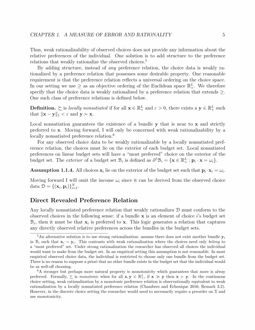
Thus, weak rationalizability of observed choices does not provide any information about therelative preferences of the individual. One solution is to add structure to the preferencerelations that weakly rationalize the observed choices.5
By adding structure, instead of any preference relation, the choice data is weakly ra-tionalized by a preference relation that possesses some desirable property. One reasonablerequirement is that the preference relation reflects a universal ordering on the choice space.In our setting we use ≥ as an objective ordering of the Euclidean space RL
+. We thereforespecify that the choice data is weakly rationalized by a preference relation that extends ≥.One such class of preference relations is defined below.
Definition. % is locally nonsatiated if for all x ∈ RL+ and ε > 0, there exists a y ∈ RL
+ suchthat ‖x− y‖1 < ε and y � x.
Local nonsatiation guarantees the existence of a bundle y that is near to x and strictlypreferred to x. Moving forward, I will only be concerned with weak rationalizability by alocally nonsatiated preference relation.6
For any observed choice data to be weakly rationalizable by a locally nonsatiated pref-erence relation, the choices must lie on the exterior of each budget set. Local nonsatiatedpreferences on linear budget sets will have a “most preferred” choice on the exterior of thebudget set. The exterior of a budget set Bi is defined as ∂↑Bi = {x ∈ RL
+ : pi · x = ωi}.
Assumption 1.1.4. All choices xi lie on the exterior of the budget set such that pi ·xi = ωi.
Moving forward I will omit the income ωi since it can be derived from the observed choicedata D = {(xi,pi)}Ni=1.
Direct Revealed Preference Relation
Any locally nonsatiated preference relation that weakly rationalizes D must conform to theobserved choices in the following sense: if a bundle x is an element of choice i’s budget setBi, then it must be that xi is preferred to x. This logic generates a relation that capturesany directly observed relative preferences across the bundles in the budget sets.
5An alternative solution is to use strong rationalization: assume there does not exist another bundle yi
in Bi such that xi ∼ yi. This contrasts with weak rationalization where the choices need only belong toa “most preferred” set. Under strong rationalization the researcher has observed all choices the individualwould want to make from the budget set. In an empirical setting this assumption is not reasonable. In mostempirical observed choice data, the individual is restricted to choose only one bundle from the budget set.There is no reason to suppose a priori that no other bundle exists in the budget set that the individual wouldbe as well-off choosing.
6A stronger but perhaps more natural property is monotonicity which guarantees that more is alwaypreferred. Formally, % is monotonic when for all x,y ∈ RL
+, if x � y then x � y. In the continuouschoice setting, weak rationalization by a monotonic preference relation is observationally equivalent to weakrationalization by a locally nonsatiated preference relation (Chambers and Echenique 2016; Remark 3.2).However, in the discrete choice setting the researcher would need to necessarily require a preorder on X anduse monotonicity.

CHAPTER 1. A MEASURE OF ERROR AND RATIONALITY 6
Definition. The observed choice xi is direct revealed preferred to x for any x ∈ Bi.
The direct revealed preference relation is derived from the observed choice data D and isdenoted by R0
D. The binary relation R0D is defined for all bundles in the union of the budget
sets⋃iBi. The direct revealed preference relation does not capture the dominance ordering
of the choice space. The strict direct revealed preference relation P 0D does just that.
Definition. xi is strictly direct revealed preferred to x if x ∈ Bi \ {∂↑Bi}
The condition x ∈ Bi is commonly written as pi · xi ≥ pi · x. Since choices are assumedto be on the exterior of the budget set (Assumption 1.1.4), this condition is equivalent toωi ≥ pi · x. Similarly, xi �R x if pi · xi > pi · x.
1.2 GARP and Afriat’s Theorem
Despite its name, the direct revealed preference relation R0D is not necessarily transitive or
complete. If it is both, then the choice data D is rationalizable by the directly revealedpreference relation R0
D.However, directly revealed preferences are usually incomplete, since there are many bun-
dles that are not compared under R0D. For example, if x ∈ B1/B2 and y ∈ B2/B1 then it is
not the case that xR0Dy or that yR0
Dx, meaning that R0D is not complete. So the problem of
checking if any preference relation weakly rationalizes the observed choice data D amounts tocompleting the directly revealed preference relation R0
D in a way that preserves transitivity(Chambers and Echenique (2016) p. 36).
The General Axiom of Revealed Preferences (GARP) provides a testable condition on theobserved choice data D. The condition checks if it is possible to extend the directly revealedpreference relation using its transitive closure, without introducing violations of transitivity.
Axiom (GARP). The directly revealed preference relation R0D satisfies the general axiom of
revealed preference if there does not exist a sequence (k) : {1, ..., N} 7→ {1, ..., K} such that
x(1)R0Dx(2), x(2)R
0Dx(3), ... x(K−1)R
0Dx(K), x(K)P
0Dx(1).
GARP is equivalent to saying that for any sequence {(x(1),p(1)); (x(2),p(2)); ...; (x(K),p(K))}from the choice data D, if {p(1) · x(1) ≥ p(1) · x(2)}, ..., {p(K−1) · x(K−1) ≥ p(K−1) · x(K)} and{p(K) · x(K) ≥ p(K) · x(1)}, then the inequalities must hold with equality.
Afriat’s theorem results in equivalence between finite continuous choice data satisfyingGARP, and the existence of a locally non-satiated weak rationalization (Afriat 1967; Diewert1973).
Theorem 1.2.1 (Afriat). Let X be a convex consumption space and D = {(xi,pi)}Ni=1 be afinite set of choice data. The following are equivalent:
(1) D has a locally non-satiated weak rationalization
CHAPTER 1. A MEASURE OF ERROR AND RATIONALITY 7
(2) R0D satisfies GARP
(3) There exist strictly positive numbers Ui and λi, ∀i such that Ui ≤ Uj + λjpj · (xi−xj)(4) D has a continuous, concave, and strictly monotonic rationalization u : X 7→ R
The equivalence of (1) and (2) guarantees the existence of a weakly rationalizing preferencerelation that is locally nonsatiated. (4) further extends the weak rationalization to guaranteethe rationalization of the individual’s choices with a model of utility maximization. A utilityfunction u maps every element in X to a real number in R and is said to rationalize apreference relation % if the mapping of u conforms with the weak ordering of %. (3) providesa set of inequalities that effectively construct such a utility function and also provide a setof linear inequalities that are easily solved. For a similar result in generalized choice settingssee Nishimura, Ok, and Quah (2016).
This paper proceeds by focusing on condition (2), namely GARP using the directlyrevealed preference relation, thereby accommodating a broad set of choice settings.
1.3 Revealed Preference Graph
The directly revealed preference relation %R is constructed to test whether the observedchoice data are weakly rationalizable by a locally nonsatiated preference relation. It is usefulto consider %R as one realization out of a set of feasible orderings. To characterize this spaceI borrow notation from the literature on graph theory.
The important insight from Afriat’s theorem is that weak rationalizability can be testedusing a finite number of conditions [EDITS NEED TO BE CONTINUED AFTER HERE]holds for the direct revealed preference relation on the N observed choices in D.
The Directly Revealed Preference as a Directed Graph
The directly revealed preference relation %R as defined in Section 1.1 can also be representedas a directed graph G := (V,E). The set of labeled vertices V = {1, ..., N} represents theN observed choices {xi}Ni=1. Each directed edge is an ordered pair of vertices (j, i) where(j, i) ∈ E if and only if xj %R xi. In subsequent sections of the paper I often represent thedirectly revealed preference graph with a {0, 1}-valued adjacency matrix R of size N × N .The row j and column i element of R is rji. The element rji is 1 whenever (j, i) ∈ E
or equivalently whenever xi %R xj. By definition, every choice is revealed preferred toitself, so rii = 1 always. These equivalent representations of the directly revealed preferredpreference relation are outlined in Table 1.1. For simplicity I call the R matrix “the revealedpreference”.7
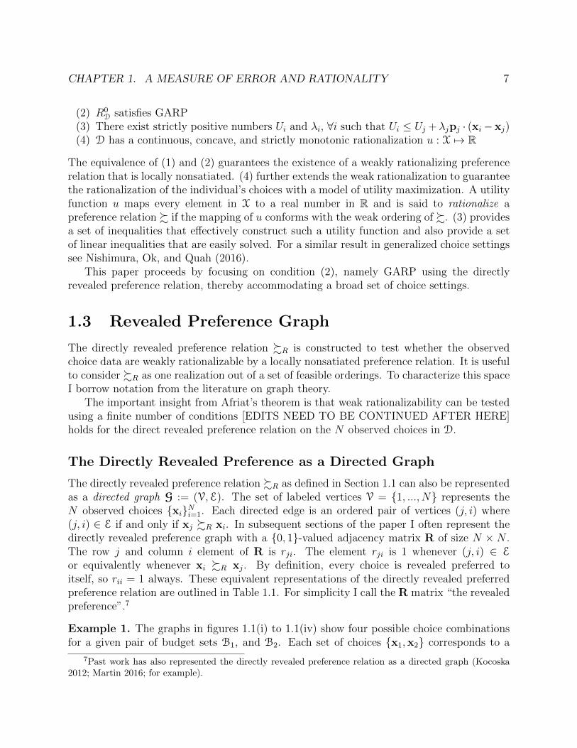
Example 1. The graphs in figures 1.1(i) to 1.1(iv) show four possible choice combinationsfor a given pair of budget sets B1, and B2. Each set of choices {x1,x2} corresponds to a
7Past work has also represented the directly revealed preference relation as a directed graph (Kocoska2012; Martin 2016; for example).
CHAPTER 1. A MEASURE OF ERROR AND RATIONALITY 8
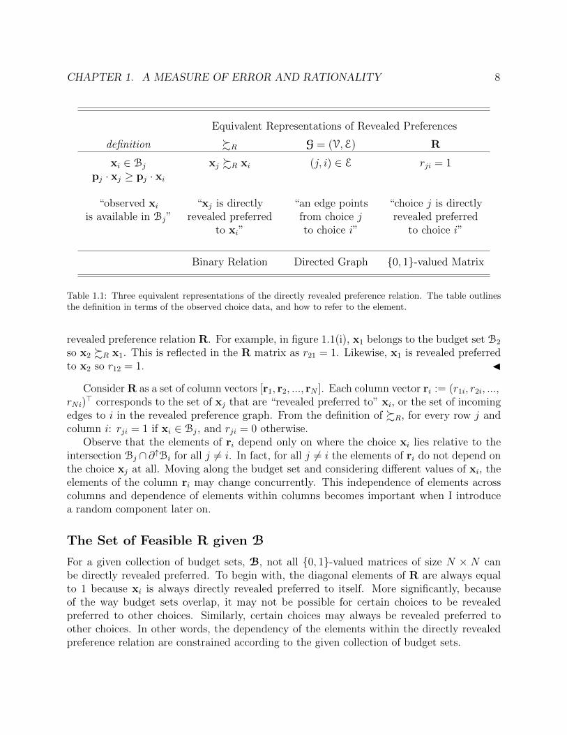
Equivalent Representations of Revealed Preferences
definition %R G = (V,E) R
xi ∈ Bj
pj · xj ≥ pj · xixj %R xi (j, i) ∈ E rji = 1
“observed xi “xj is directly “an edge points “choice j is directlyis available in Bj” revealed preferred from choice j revealed preferred
to xi” to choice i” to choice i”
Binary Relation Directed Graph {0, 1}-valued Matrix
Table 1.1: Three equivalent representations of the directly revealed preference relation. The table outlinesthe definition in terms of the observed choice data, and how to refer to the element.
revealed preference relation R. For example, in figure 1.1(i), x1 belongs to the budget set B2
so x2 %R x1. This is reflected in the R matrix as r21 = 1. Likewise, x1 is revealed preferredto x2 so r12 = 1. J
Consider R as a set of column vectors [r1, r2, ..., rN ]. Each column vector ri := (r1i, r2i, ...,rNi)
> corresponds to the set of xj that are “revealed preferred to” xi, or the set of incomingedges to i in the revealed preference graph. From the definition of %R, for every row j andcolumn i: rji = 1 if xi ∈ Bj, and rji = 0 otherwise.
Observe that the elements of ri depend only on where the choice xi lies relative to theintersection Bj ∩ ∂↑Bi for all j 6= i. In fact, for all j 6= i the elements of ri do not depend onthe choice xj at all. Moving along the budget set and considering different values of xi, theelements of the column ri may change concurrently. This independence of elements acrosscolumns and dependence of elements within columns becomes important when I introducea random component later on.
The Set of Feasible R given B
For a given collection of budget sets, B, not all {0, 1}-valued matrices of size N × N canbe directly revealed preferred. To begin with, the diagonal elements of R are always equalto 1 because xi is always directly revealed preferred to itself. More significantly, becauseof the way budget sets overlap, it may not be possible for certain choices to be revealedpreferred to other choices. Similarly, certain choices may always be revealed preferred toother choices. In other words, the dependency of the elements within the directly revealedpreference relation are constrained according to the given collection of budget sets.
CHAPTER 1. A MEASURE OF ERROR AND RATIONALITY 9
𝐱1
𝐱2
ℬ2
ℬ1
𝐑 =1 11 1
(i)
𝐱1 𝐱2
ℬ2
ℬ1
𝐑 =1 01 1
(ii)
𝐱1𝐱2
ℬ2
ℬ1
𝐑 =1 10 1
(iii)
𝐱2
ℬ2
ℬ1
𝐱1
𝐑 =1 00 1
(iv)
Figure 1.1: Each figure shows a possible set of choices arising from a pair of budget sets B1 and B2. Theaccompanying directly revealed preference relation R arises from the location of x1 and x2 relative to B1∩B2.There are no other feasible directly revealed preference relations from these two budget sets.
To characterize the space of feasible directly revealed preference relations, I define theset of feasible columns for each budget set. Fixing the collection of budget sets B, non-overlapping subsets of ∂↑Bi map to different columns of R. The subsets of ∂↑Bi are definedaccording to intersections of ∂↑Bi with the remaining budget sets.8 This process is illustratedas it applies to example 1.
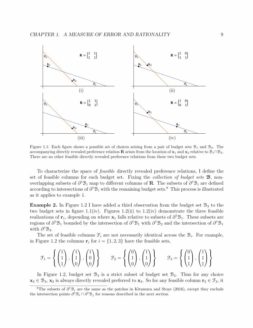
Example 2. In Figure 1.2 I have added a third observation from the budget set B3 to thetwo budget sets in figure 1.1(iv). Figures 1.2(ii) to 1.2(iv) demonstrate the three feasiblerealizations of r1, depending on where x1 falls relative to subsets of ∂↑B1. These subsets areregions of ∂↑B1 bounded by the intersection of ∂↑B1 with ∂↑B2 and the intersection of ∂↑B1
with ∂↑B3.The set of feasible columns Fi are not necessarily identical across the Bi. For example,
in Figure 1.2 the columns ri for i = {1, 2, 3} have the feasible sets,
F1 =
1
11
,
110
,
100
F2 =
0
10
,
110
F3 =
0
11
,
111
In Figure 1.2, budget set B3 is a strict subset of budget set B2. Thus for any choice
x3 ∈ B3, x2 is always directly revealed preferred to x3. So for any feasible column r3 ∈ F3, it
8The subsets of ∂↑Bi are the same as the patches in Kitamura and Stoye (2016), except they excludethe intersection points ∂↑Bi ∩ ∂↑Bj for reasons described in the next section.

CHAPTER 1. A MEASURE OF ERROR AND RATIONALITY 10
𝐱2
𝐱1𝐱3
ℬ2
ℬ1ℬ3
𝐑 =1 0 10 1 10 0 1
(i)
ℬ3
ℬ2
ℬ1
𝐑 =1 − −1 − −1 − −
(ii)
ℬ3
ℬ2
ℬ1
𝐑 =1 − −1 − −0 − −
(iii)
ℬ3
ℬ2
ℬ1
𝐑 =1 − −0 − −0 − −
(iv)
ℬ3
ℬ2
ℬ1
𝐑 =− 0 −− 1 −− 0 −
(v)
ℬ3
ℬ2
ℬ1
𝐑 =− 1 −− 1 −− 0 −
(vi)
ℬ3
ℬ2
ℬ1
𝐑 =− − 0− − 1− − 1
(vii)
ℬ3
ℬ2
ℬ1
𝐑 =− − 1− − 1− − 1
(viii)
Figure 1.2: Not all preference relations R are feasible. (i) adds a choice from B3 to figure 1.1(iv). (ii) -(iv) show the three feasible realizations of r1 depending on which subset of the budget set B1 the choicex1 belongs to. (v) - (vi) and (vii) - (viii) are the two feasible realizations of r2 and r3 respectively. SinceB3 ⊂ B2, x2 %R x3 and ¬(x3 %R x3), any x2 ∈ B2 and any x3 ∈ B3. So for any feasible R, it must be thatr23 = 1 and r32 = 1 always.
must always be the case that r23 = 1. This means that if R has the column r3 = (0, 0, 1)>,then R would not be a feasible revealed preference relation. In contrast, for any choicex2 ∈ B2, x3 is never revealed preferred to x2. So every feasible column r2 has r32 = 0.

CHAPTER 1. A MEASURE OF ERROR AND RATIONALITY 11
Indeed these restrictions can be seen in the feasible sets F2 and F3. J
I denote each subset of the exterior of the budget line ∂↑Bi as Xki , with which we associate
Wk an element of the power set 2{1,..,N}. Each Xki is defined as the intersection of ∂↑Bi with
all budget sets indexed by Wk intersected with the complement of all remaining budget sets.Formally,
Xki = ∂↑Bi
⋂n∈Wk
Bn
⋂m∈Wc
k\{i}
Bcm
Note that for any i, the union of Xki over all k is precisely ∂↑Bi. Additionally, each Xk
i is
mutually exclusive to all other such subsets of ∂↑Bi, that is Xki ∩ Xk
′
i = ∅ for all k 6= k′.
Many of the Xki are empty, so we retain only nonempty Xk
i reindexing them by k =1, ..., Ki. The total number of subsets becomes Ki. With a finite number of observations N ,the total number of subsets Ki ≤ 2(N−1) is also finite.
By definition of R, any choice xi in Xki has the same “revealed preferred to” column ri.
Although I do not prove it formally, the following is an intuitive consequence of the definitionof Xk
i .
Claim 1.3.1. Let Fi denote the set of feasible “revealed preferred to i” columns ri. EachXki corresponds to a unique element rki ∈ Fi and |Fi| = Ki.
The set of all feasible preference relations is F := F1×F2× ...×FN . There are 2N×(N−1)
possible N ×N binary matrices with a diagonal of 1. The number of feasible R is generallymuch smaller, and is counted as |F| =
∏Ni=1Ki. The exact number of feasible R for a given
B depends on the specific way the budget sets intersect.Generally, the more the budget sets intersect each other in different places, the more
feasible columns there are and consequently the more feasible graphs there are. In example 1there are 64 possible N × N binary matrices with 1s on the diagonal. But there are only3 × 2 × 2 = 12 feasible R. In a related paper Deb and Pai (2014) explore the geometry ofrevealed preferences in the continuous choice setting.
Acyclicity of R and GARP
I now present sufficient assumptions under which acyclicity, a property of R, becomes equiv-alent to GARP. This equivalence means that the econometrics can focus on the revealedpreference relation represented by R.
A cycle in a directed graph G is a set of edges that create a path from i and back to ipossibly through a subset of other vertices in V. In the adjacency matrix representation Rsuch a cycle corresponds to a sequence of elements (k) : {1, ..., N} 7→ {1, ..., K} such thatr(1)(2) = 1, r(2)(3) = 1, ..., r(K−1)(K) = 1 and r(K)(1) = 1.
Definition. The graph R is acyclic if it does not contain any cycles. R is cyclic if it containsat least one cycle.

CHAPTER 1. A MEASURE OF ERROR AND RATIONALITY 12
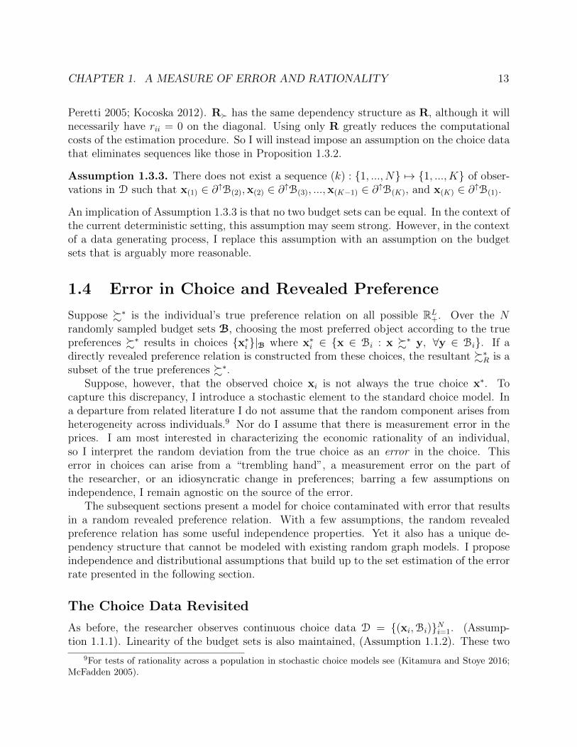
Example. Figure 1.3 shows an example of a cycle between three vertices. This cycle isequivalent to a revealed preference relation in which x1 %R x2, x2 %R x3, and x3 %R x1.If these were the only observations, then the graph G = (V,E) is the set of vertices labeledaccording to the observation index {1, 2, 3}, and the set of directed edges {(1, 2), (2, 3), (3, 1)}.Both the graph G and the associated adjacency matrix R are cyclic. J
1
𝐑 =1 1 00 1 11 0 1
𝐱1 ≿𝑅 𝐱2
𝐱2 ≿𝑅 𝐱3
𝐱3 ≿𝑅 𝐱1
𝒢 = 𝒱, ℰ
ℰ = 1,2 ; 2,3 ; 3,1
𝒱 = 1, 2, 3
2 3
Figure 1.3: The directed graph consisting of 3 vertices and a single cycle across all vertices. The colors linkeach directed edge (j, i) with a pair of“revealed preferred to” observations xj %R xi and rji an element ofR.
In the context of the directly revealed preference relation, whenever R is acyclic theredoes not exist a sequence (k) : {1, ..., N} 7→ {1, ..., K} such that x(1) %R x(2), x(2) %R x(3),...,x(K−1) %R x(K), and also x(K) %R x(1). The crucial difference between acyclicity and GARPis in the missing strict relation �R on the last pair x(K) and x(1) in the cycle. GARP doesnot rule out complete indifference among all the choices in a cycle, while acyclicity does.
The observational divergence of acyclicity and GARP occurs when for a sequence ofchoices each lies in the respective intersection of theirs and the next budget set’s exterior.Since GARP allows for indifference, if xi is chosen from the budget set exterior of ∂↑Bj
then xj is not strictly preferred to xi. When a set of choices each belong to other budgetset exteriors in sequence, then there is a cycle in R, but GARP is not violated. In allother instances GARP and acyclicity coincide because either a cycle does not exist, meaningGARP is satisfies, or a cycle exists in a way that violates GARP.
Proposition 1.3.2. Suppose there does not exist a sequence (k) : {1, ..., N} 7→ {1, ..., K}such that x(2) ∈ ∂↑B(1),x(3) ∈ ∂↑B(2), ...,x(K) ∈ ∂↑B(K−1), and x(1) ∈ ∂↑B(K). Then either
(i) %R satisfies GARP and R is acyclic, or(ii) %R violates GARP and R is cyclic.
A proof and a detailed example explaining the case when N = 2 is provided in appendix A.1One way to deal with the above divergence is to additionally construct a “strictly directly
preferred” relation graph based on �R. Some empirical papers construct R� (Jones and De
CHAPTER 1. A MEASURE OF ERROR AND RATIONALITY 13
Peretti 2005; Kocoska 2012). R� has the same dependency structure as R, although it willnecessarily have rii = 0 on the diagonal. Using only R greatly reduces the computationalcosts of the estimation procedure. So I will instead impose an assumption on the choice datathat eliminates sequences like those in Proposition 1.3.2.
Assumption 1.3.3. There does not exist a sequence (k) : {1, ..., N} 7→ {1, ..., K} of obser-vations in D such that x(1) ∈ ∂↑B(2),x(2) ∈ ∂↑B(3), ...,x(K−1) ∈ ∂↑B(K), and x(K) ∈ ∂↑B(1).
An implication of Assumption 1.3.3 is that no two budget sets can be equal. In the context ofthe current deterministic setting, this assumption may seem strong. However, in the contextof a data generating process, I replace this assumption with an assumption on the budgetsets that is arguably more reasonable.
1.4 Error in Choice and Revealed Preference
Suppose %∗ is the individual’s true preference relation on all possible RL+. Over the N
randomly sampled budget sets B, choosing the most preferred object according to the truepreferences %∗ results in choices {x∗i }|B where x∗i ∈ {x ∈ Bi : x %∗ y, ∀y ∈ Bi}. If adirectly revealed preference relation is constructed from these choices, the resultant %∗R is asubset of the true preferences %∗.
Suppose, however, that the observed choice xi is not always the true choice x∗. Tocapture this discrepancy, I introduce a stochastic element to the standard choice model. Ina departure from related literature I do not assume that the random component arises fromheterogeneity across individuals.9 Nor do I assume that there is measurement error in theprices. I am most interested in characterizing the economic rationality of an individual,so I interpret the random deviation from the true choice as an error in the choice. Thiserror in choices can arise from a “trembling hand”, a measurement error on the part ofthe researcher, or an idiosyncratic change in preferences; barring a few assumptions onindependence, I remain agnostic on the source of the error.
The subsequent sections present a model for choice contaminated with error that resultsin a random revealed preference relation. With a few assumptions, the random revealedpreference relation has some useful independence properties. Yet it also has a unique de-pendency structure that cannot be modeled with existing random graph models. I proposeindependence and distributional assumptions that build up to the set estimation of the errorrate presented in the following section.
The Choice Data Revisited
As before, the researcher observes continuous choice data D = {(xi,Bi)}Ni=1. (Assump-tion 1.1.1). Linearity of the budget sets is also maintained, (Assumption 1.1.2). These two
9For tests of rationality across a population in stochastic choice models see (Kitamura and Stoye 2016;McFadden 2005).

CHAPTER 1. A MEASURE OF ERROR AND RATIONALITY 14
assumptions imply that the prices and income for each Bi are both observable to the re-searcher. In lab experiments with linear and continuous budget sets these assumptions easilyhold, but with observational data they may not.
Example. A researcher is interested in studying the rationality of consumers with super-market scanner data. The amount purchased and the price per unit are both known to theresearcher. However, Assumption 1.1.1 is not met since prices on un-purchased items areunknown. The researcher gets access to price data on all goods from the supermarket. Un-der the assumption that the consumer spent his entire grocery budget (Assumption 1.1.4), alinear budget set can be constructed. Any coupons at the register, or unexpected sales canbe accounted for with savings. J
In addition to observability, there are two subtle but important assumptions that needto hold on the nature of truth and error. The first states explicitly that the error arises inthe observed choices, and the second states that the true choice is deterministic conditionalon the budget set.
Assumption 1.4.1. Error arises in the observed choices.
Assumption 1.4.2. The true choice x∗i is deterministic conditional on the observed budgetset Bi.
Here error manifests as random noise in the observed choices. Again, these assumptionshold easily in lab experiments where the researcher creates the budget sets, however inobservational data they may not. Extending this work to settings with noisy budget is leftto the interested reader. Such an extension will likely require a known (or estimated) errordistribution on the budget sets. Using this distribution, the researcher
Example. A researcher is interested in studying the rationality of consumers on a broadrange of aggregated goods: food, medical care, transportation, housing, etc. The researcheris interested in using household retail data coupled with household income (e.g. NielsenConsumer Panels). Often household income includes some measurement error: either thereported post-tax income is incorrect, or because the researcher uses gross income and doesnot know the correct tax rate to apply. The observed budget set is noisy, meaning that x∗i |Bi
is a random variable, violating Assumption 1.4.2. J
The Contaminated Choice Model
I define a model in which the observed choices are contaminated randomly (Manski 2003).For each observed choice xi ∈ Bi, with probability (1−π) an error-free choice x∗i is observed.With probability π, a random data error ui is observed instead. Each observed choice xi is
CHAPTER 1. A MEASURE OF ERROR AND RATIONALITY 15
thus a random variable decomposed as10,11
xi = (1− zi)x∗i + ziui. (1.1)
Assumption 1.4.3. The unobserved indicator of an error zi ∈ {0, 1} is a Bernoulli randomvariable with an unknown error rate P (z = 1) = π.
Each x∗i is unknown to the researcher and deterministic conditional on the budget setBi (Assumption 1.4.2). Conditional on Bi, the unobserved random error ui is distributedaccording to some probability distribution Fui
.12
Assumption 1.1.4 must hold for weak rationalizability to have meaning, so the true choicesx∗i lie on the exterior of the budget set, ∂↑Bi. For the observed revealed preference relationpresented in the next section, it must also be the case that each ui belongs to the exteriorof the budget set.
Assumption 1.1.4 (extended). Each error-free choice x∗i and error ui belong to the exteriorof the budget set ∂↑Bi
From the extension of Assumption 1.1.4 above, the support of the distribution Fuiis
defined to be ∂↑Bi. It also naturally follows that the observed choice xi is also in theexterior of the budget set ∂↑Bi. A discussion of the distribution on the errors in choice willappear after a discussion of the revealed preference relation.
As promised, another version of Assumption 1.3.3 can be introduced: cycles that obser-vationally differentiate acyclicity from GARP occur with zero probability.
Assumption 1.4.4. Conditional on B, the probability is zero that there exists a sequence(k) : {1, ..., N} 7→ {1, ..., K} of observations in D such that x(1) ∈ ∂↑B(2),x(2) ∈ ∂↑B(3), ...,x(K−1) ∈ ∂↑B(K), and x(K) ∈ ∂↑B(1).
In the continuous choice setting, Assumption 1.4.4 requires the distribution on each errorto have a zero probability on the intersection of two budget sets. The assumption also impliesthat no two budget set exteriors are identical, ∂↑Bi 6= ∂↑Bj. So the errors in the choices uiare not identically distributed conditional on B.
Assumption 1.4.4 also requires that such a sequence cannot exist in the error-free choicesx∗i . Since x∗i is deterministic conditional on Bi, Assumption 1.4.4 is a strengthening ofAssumption 1.3.3.
10The standard contamination model in Manski (2003) (p.60) aims to partially identify the probability oferror-free realizations, P (x∗|z = 0). The distribution of interest is that on the data errors themselves. ThusI reverse zi and (1− zi) in the specification, as well as the definition of π.
11Standard models of stochastic choice that relate the error to the utility do not apply since this estimationprecludes the existence of a utility representation for choice.
12The data convolution model xi = x∗i + ε can be written as a contaminated choice model. Assume π = 1and the choice error is ui = x∗i + εi where εi ∼iid N (0, σ2). The distribution is now parameterized by σ2,which is less interpretable and is more complicated to work with.

CHAPTER 1. A MEASURE OF ERROR AND RATIONALITY 16
Remark. A sufficient condition for this assumption is that the budget sets be exogenouslyand randomly chosen from a suitably large space of possible budget sets. In many laboratoryexperiments eliciting choices from linear budget sets, this condition holds. It will not holdin a dynamic design experiment in which the budget sets are generated so as to intersect ata previously observed choice (as proposed in Andreoni, Gillen, and Harbaugh (2013)). Inapplied settings, if the prices can be treated as exogenous and random with respect to theindividual’s choices, then the assumption will also hold. In settings with endogenous budgetsets, the assumption may still be reasonable but should be verified by the researcher.
Random Revealed Preferences
A revealed preference relation constructed from a contaminated choice data is also contam-inated with error.
As explained in Section 1.3 each “revealed preferred to i” column is constructed fromthe collection of budget sets B and the observed choice xi alone. This is denoted asr = (r1i, r2i, ..., rNi)
>. From the contaminated choice model in (1.1), whenever zi is 0,the observed choice xi is the error-free choice x∗i . So the observed “revealed preferred toi” column ri is also error-free. This error-free column r∗i is denoted (r∗1i, r
∗2i, ..., r
∗Ni)>. Each
element r∗ji is 1 whenever x∗i ∈ Bj.If an error occurs then zi is 1. The observed choice xi is therefore an error ui, and the
observed “revealed preferred to i” column ri is also an error. The error column ei is denotedby (e1i, e2i, ...eNi)
>, where each element eij is 1 whenever ui ∈ Bj. Table 1.2 summarizes theconstruction of ri.
Unobserved Observed
zi xi ri rij
error-free at i zi = 0 xi is x∗i ri is r∗i r∗ij = 1 iff x∗i ∈ Bj
an error has zi = 1 xi is ui ri is ei eij = 1 iff ui ∈ Bj
occurred at i
Table 1.2: The choice xi is observed and used to construct the “revealed preferred to i” column ri from thischoice. However the unobserved indicator zi affects whether the researcher observes the error-free choice x∗ior an error ui. Correspondingly the “revealed preferred to i” column is either error-free ri or an error ei.
The observed revealed preference relation R = [r1, r2, ..., rN ] is a set of N randomlycontaminated N × 1 columns. For each “revealed preferred to i” column ri, with probability(1 − π) an error-free column r∗i is observed, and with probability π an error column ei isobserved.
Since xi, x∗i , and ui are all elements of ∂↑Bi by Assumption 1.1.4, the subsequent “re-vealed to i” columns ri, r
∗i , ei are all feasible and therefore elements of Fi per Claim 1.3.1.

CHAPTER 1. A MEASURE OF ERROR AND RATIONALITY 17
Further, each“revealed preferred to i” column ri ∈ R is constructed from the observed choicexi as the random variable (N × 1 column vector)
ri = r∗i (1− zi) + ei(zi). (1.2)
From Assumption 1.4.3 the zi ∼iid Bernoulli (π). Conditional on the collection of budgetsets B, each r∗i is deterministic but unknown (Assumption 1.4.2). The random variable eiis distributed according to a probability mass function fei on the finite discrete support Fi.
The probability mass function (pmf) of the errors fei is derived directly from the distri-bution function Fui
of the errors in choice ui. Integrating the error distribution Fuiover each
subset Xki of ∂↑Bi gives the probability that ei = rki . Here rki is the column in the feasible
set Fi that results from the choices in the subset Xki . Repeating this for all k ∈ {1, ..., Ki}
yields the probability function for ei. That is,
Definition. Given B, for any observation i and for all k ∈ {1, ..., Ki},
fei(k) := P(ei = rki
)= P
(ui ∈ Xk
i
)=
∫x∈Xk
i
dFui(x)
As mentioned before, Assumption 1.4.4 implies that ∂↑Bi 6= ∂↑Bj, in which case the feasiblesets for two columns i and j are also not the same, i.e. Fi 6= Fj. Consequently, the errorcolumns in the revealed preference relation ei are not identically distributed conditional onB.
Example 2 (continued). Figure 1.4 shows this integration process for B1 from Figure 1.2.In figure 1.4(i) an error density dFu1 lies on the support ∂↑B1. The density dFu1 is segmentedwhen the three subsections X1
1,X21, and X3
1 are overlaid onto the exterior of the budget set,as infigure 1.4(iii) . Taking as an example k = 2, the integral of dFu1 on X2
1 gives the valueof fe1(2), which is the probability that r1 = r21. Figure 1.4(ii) shows the resultant probabilityfe1 of the error columns on the support F1. J
A Unique Dependency Structure
The revealed preference relation R = [r1, ..., rN ] is a random analogue of the nonrandomadjacency matrix introduced in Section 1.3 and the direct revealed preference relation %R
introduced in Section 1.1.Since R is constructed directly from the observed choices, random error is incorporated
in a way that accounts for the inherent dependency structure of the preference relation.Recall that the elements within each “revealed to i” column ri depend only on the choicexi conditional on the collection of budget sets B. This dependency shows up in the randomgraph R from (1.2) because it is constructed in the same way as the revealed preferencerelation in the deterministic choice setting. The location of the observed choice xi on ∂↑Bi
determines which column is observed, out of the feasible set Fi. Thus the elements of thecolumn rij are not necessarily independent.
CHAPTER 1. A MEASURE OF ERROR AND RATIONALITY 18
𝐮1 ∈ 𝜕↑ℬ1
𝑑𝐹𝐮1
(i)
ℱ1
𝑓𝐞1
100
111
110
(ii)
𝒳12
𝜕↑ℬ1
𝐫12 =
110
𝒳11 𝒳1
3
𝑑𝐹𝐮1
(iii)
ℱ1
𝑓𝐫1
100
111
110
𝐫1∗
(iv)
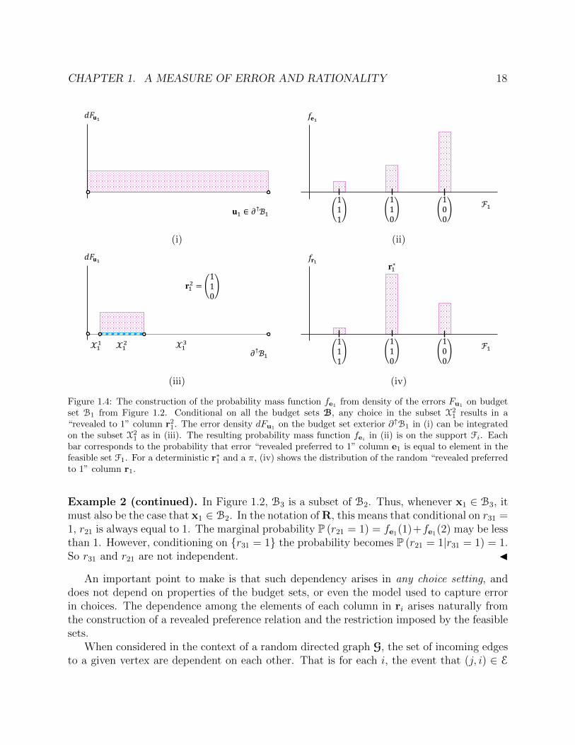
Figure 1.4: The construction of the probability mass function fe1 from density of the errors Fu1 on budgetset B1 from Figure 1.2. Conditional on all the budget sets B, any choice in the subset X2
1 results in a“revealed to 1” column r21. The error density dFu1
on the budget set exterior ∂↑B1 in (i) can be integratedon the subset X2
1 as in (iii). The resulting probability mass function feiin (ii) is on the support Fi. Each
bar corresponds to the probability that error “revealed preferred to 1” column e1 is equal to element in thefeasible set F1. For a deterministic r∗1 and a π, (iv) shows the distribution of the random “revealed preferredto 1” column r1.
Example 2 (continued). In Figure 1.2, B3 is a subset of B2. Thus, whenever x1 ∈ B3, itmust also be the case that x1 ∈ B2. In the notation of R, this means that conditional on r31 =1, r21 is always equal to 1. The marginal probability P (r21 = 1) = fe1(1)+fe1(2) may be lessthan 1. However, conditioning on {r31 = 1} the probability becomes P (r21 = 1|r31 = 1) = 1.So r31 and r21 are not independent. J
An important point to make is that such dependency arises in any choice setting, anddoes not depend on properties of the budget sets, or even the model used to capture errorin choices. The dependence among the elements of each column in ri arises naturally fromthe construction of a revealed preference relation and the restriction imposed by the feasiblesets.
When considered in the context of a random directed graph G, the set of incoming edgesto a given vertex are dependent on each other. That is for each i, the event that (j, i) ∈ E

CHAPTER 1. A MEASURE OF ERROR AND RATIONALITY 19
and (k, i) ∈ E are typically dependent on each other, a dependency which rules out the use ofrandom graph models with independent edge probabilities, in the spirit of the Erdos-Renyirandom graph .
In contrast, independence across observations is a reasonable possibility. In the determin-istic case presented in Sections 1.1 and 1.3 each “revealed preferred to i” column ri is derivedwithout any of the other observed choices xj. It is in fact possible to make an assumptiondirectly on the contaminated choice model from (1.1), which leads to independence acrossthe columns of R.
By Assumption 1.4.3, the indicators of an error zi are distributed as Bernoulli randomvariables, and are thus independent of each other, and independent of the error ui. ByAssumption 1.4.2, the error-free choice x∗i is deterministic conditional on B, all that remainsis to impose an independence condition on the errors ui:
Assumption 1.4.5. ∀i 6= j, ui ⊥ uj conditional on B.
The assumption above guarantees that the error from one observation does not relate to anerror from another observation.
This independence assumption leads to independence among the observed choices xi.
Proposition 1.4.6. Under Assumptions 1.4.2, 1.4.3 and 1.4.5, ∀i 6= j xi ⊥ xj conditionalon B.
The independence of the choice errors ui leads directly to the independence of errorcolumns ei. This is because the probability function of the revealed preference errors feiderives directly from the distribution of the choice errors Fui
. The indicators of an error ziin (1.2) are the same independent Bernoulli random variables as before, and the error-freecolumns r∗i are deterministic conditional on B. This gives independence across the columnsri of the observed revealed preference relation.
Proposition 1.4.7. Under Assumptions 1.4.2, 1.4.3 and 1.4.5, ∀i 6= j, ri ⊥ rj conditionalon B.
Known Error Distribution with Unknown Parameter
If the functional form of the error distribution Fuiis known up to a vector of parameters φ,
then the probability mass function fei can be derived as a function of φ. As a result, thedistribution of R is known up to the parameter θ = (R∗, π;φ).13
In contrast to existing literature, the parameter φ not assumed to be known (for a dis-cussion see appendix A.3). The only restriction is the cardinality of φ. While in theorythe method of moments presented in this paper may seem to provide moments that permitestimation of up to N parameters. However, in practice this is not the case. It must be that|φ| � N because higher moments rely on rare events and will not estimate accurately.
13R∗ is the adjacency matrix defined by the columns r∗i defined formally as R∗ = [r∗1, r∗2, ..., r
∗N ].
CHAPTER 1. A MEASURE OF ERROR AND RATIONALITY 20
In choosing a functional form to model the error, the researcher should account for thechoice setting and the interpreted source of the error. Unless there is a clear reason todo otherwise, it is recommended that the general shape or family of the error distributionremain the same for each ui, conditional on the support ∂↑Bi.
Example. A common interpretation of error in choice is a “trembling hand”. The observedchoice xi is close to, but not exactly equal to some true choice x∗i . This could be representedas a multi-variate normal error truncated on the support ∂↑Bi and centered at x∗i . Theprobability of observing xi decreases further away from x∗i . A few precautionary notes: thedistributional complexity |φ| increases in the dimension of the goods L, unless the scale iskept constant over all dimensions. Additionally, for such trembling had error distributionone must impose a distance metric on the choice space. Since many discrete choice settingsdo not have a well defined distance metric, a distance-dependent error is undesirable. J
For the remainder of this paper I assume a uniform error across the budget set ∂↑Bi.This is consistent with an idiosyncratic change in preferences, or perhaps even measurementerror on the part of the researcher. There is a precedent for using a uniform distributionin tests of rationality that incorporate random error (Bronars 1987; Andreoni, Gillen, andHarbaugh 2013). A uniform distribution on the budget set can also easily apply to a discretechoice setting.
Assumption 1.4.8. The errors in each choice are ui ∼ U [∂↑Bi] where U is the uniformdistribution.
Computationally, it is simple to integrate a uniform distribution across the subsets Xki for
all k ∈ {1, ..., Ki} and all i ∈ {1, ..., N}. Conditioning on each budget set Bi, the uniformdistribution on ∂↑Bi does not require any additional parameters, so φ = ∅.
1.5 A Test for Acyclic R∗
We are interested in knowing if an individuals’ choices are weakly rationalizable by a locallynon-satiated preference relation. With the introduction of error in the observed choices, theobject of interest becomes individuals’ true choices {x∗i }Ni=1. Are the true choices weaklyrationalizable by a locally non-satiated preference relation? This is equivalent to asking ifR∗ is acyclic, or equivalently (under Assumption 1.3.3) to checking GARP.
However the observed object is not necessarily R∗, but rather a realization of the randomrevealed preference relation R constructed from the individual’s observed choice data. If Rhas a cycle, can we say that R∗ is acyclic and the cycle is due to error? If R∗ is acyclic thenit belongs to the set A ⊆ F, where A is the set of acyclic feasible graphs.14 We would like to
14Among the set of feasible graphs some are acyclic and, depending on the intersections of the budgetsets, some feasible graphs are also cyclic. This result is proven for the continuous choice case in Deb and Pai(2014). Results for more general choice settings are left to the reader, but should follow from the intersectionsamong the budget sets in B.
CHAPTER 1. A MEASURE OF ERROR AND RATIONALITY 21
use a realization of R to test the null hypothesis that R∗ is acyclic against the alternativehypothesis that it is not.
H0 : R∗ ∈ A
H1 : R∗ 6∈ A
Under the econometrics model presented in the previous section, the distribution of R con-ditional on B is parameterized by θ = {R∗, π}.15 The deterministic R∗ can interpreted asthe location of the distribution about which realized values of R arise. The error rate πinteracts with the error probability mass function fei to provide a measure akin to scale ofthe distribution of R. In this framework, the hypothesis test asks if the parameter of interestR∗ belongs to a particular subset of the parameter space.
There are two obstacles to testing the null hypothesis in the context of individual choicescontaminated with error. First, only one realization of R is observed by the researcher. Thesecond difficulty is that π is unknown. In the following section I show that the distributionof R is identified by θ = (R∗, π); each unique combination of π and R∗ generate a differentdistribution for R. This means that a single observation of R is not a sufficient statisticfor estimating R∗. In fact as π approaches 1, the distribution of R under the null becomesindistinguishable from the distribution under the alternative.
For a given R∗, it is possible to estimate π. One such approach to estimation uses amethod of moments estimator that leverages the graph structure of R. Therefore, condi-tioning on R∗ being acyclic results in a set of estimates {π(R)}R∈A consistent with the nullhypothesis. The minimum of this set is interpreted as the smallest error rate necessary toaccount for the observed cycles in R when R∗ is acyclic. This method for testing the nullhypothesis is in the spirit of Varian (1985).
The set-estimation presented in this paper deviates from existing methods which rely onrepeated realizations of R or assume π is known to the researcher. A discussion of existingmethods in the framework of this paper can be found in appendix A.3.
Partial Identification of R∗
The distribution of R is identified by the unknown parameters R∗ and π. Consider the firstmoment of R, which is an N ×N matrix with elements between 0 and 1.
Eθ[R] = (1− π)R∗ + π Eφ[E].
The N × N matrix E is completely random. Each column ei of E is distributed accordingto the error probability mass function fei . Recall that the error distribution is assumedto be uniform, and thus φ = ∅. Therefore we write E[E] with the implication being thatthe expectation is taken over the distribution of E. Each row j and column i element of
15The space of possible parameters is Θ = F × [0, 1] where F is the set of all feasible graphs introducedin Section 1.3.

CHAPTER 1. A MEASURE OF ERROR AND RATIONALITY 22
E[E] is the marginal probability that eji = 1 according to i’s probability mass function fei .For simplicity of notation the marginal probability Pei (eji = 1) is denoted Pi (j). For everyfeasible column i, the element rii is equal to 1, so Pi (i) = 1 for all i. Since fei is definedon the support of feasible Fi, whenever all columns in Fi have 1 in row j, it must be thatPi (j) = 1. Therefore, r∗ji and rji are also 1. The same logic holds for marginal probabilitiesof 0.
It is desirable that each unique θ = (R∗, π) ∈ Θ yields a different Eθ[R]. As shown inProposition 1.5.3, the following two assumptions guarantee the is identification property.
Assumption 1.5.1. The parameter space Θ is such that the error rate π is less than 1.
Assumption 1.5.1 only rules out the uninteresting case where choices are completelyrandom without any relevance to the true preference R∗. This a weak assumption since themodel incorporates can still incorporate a high rate of error with π very close to 1.
Assumption 1.5.2. The distribution of errors in choices is such that E[E] 6∈ F, conditionalon B.
Assumption 1.5.2 eliminates the situation where R∗ = E[E] for any possible R∗. Thisassumption fails if and only if every fei has a probability mass of 1 on Fi, in which case thesupport of E consists of a single feasible graph in F. The edge case in which the collectionof budget sets B results in only one feasible graph is ruled out.16 A more subtle implicationof Assumption 1.5.2 is that there must be some observation i whose error distribution Fui
is positive over at least two partitions Xki and Xl
i. This assumption may be stronger in thediscrete choice setting.
Proposition 1.5.3. Under Assumptions 1.5.1 and 1.5.2, for all θ, θ ∈ Θ there does not exista pair θ 6= θ such that Eθ[R] = Eθ[R].
The identification proof and an illustrative example are given in Appendix A.2.While the distribution of R is identified by θ = (R∗, π), it is only partially identified by
R∗. Thus, when π is unknown, a single realization of R is not sufficient for determiningR∗. Instead of directly estimating R∗, I take a different approach. In the case where therealization of R has a cycle, it is possible to set-identify π conditioning on the set of R∗
being acyclic.
Graph Theory Terminology
Before proceeding with the estimation, I provide the relevant graph theory terminology.Consider two subsets of the observations, defined according to zi. The error observationshave indices Z = {i ∈ 1, ..., N : zi = 1}, while the error-free observations are the complement
16For a discussion of how to address the problem of demand prediction in cases where the budget sets donot intersect see the literature related to Blundell, Browning, and Crawford (2003).
CHAPTER 1. A MEASURE OF ERROR AND RATIONALITY 23
𝐑 =
𝐑𝒵𝑐∗ 𝐄𝒵
𝒵𝑐 𝒵
(i)
𝐑 =
𝐑∗ 𝒵𝑐
𝒵𝑐 𝒵
𝒵𝑐
𝒵𝐄 𝒵
(ii)
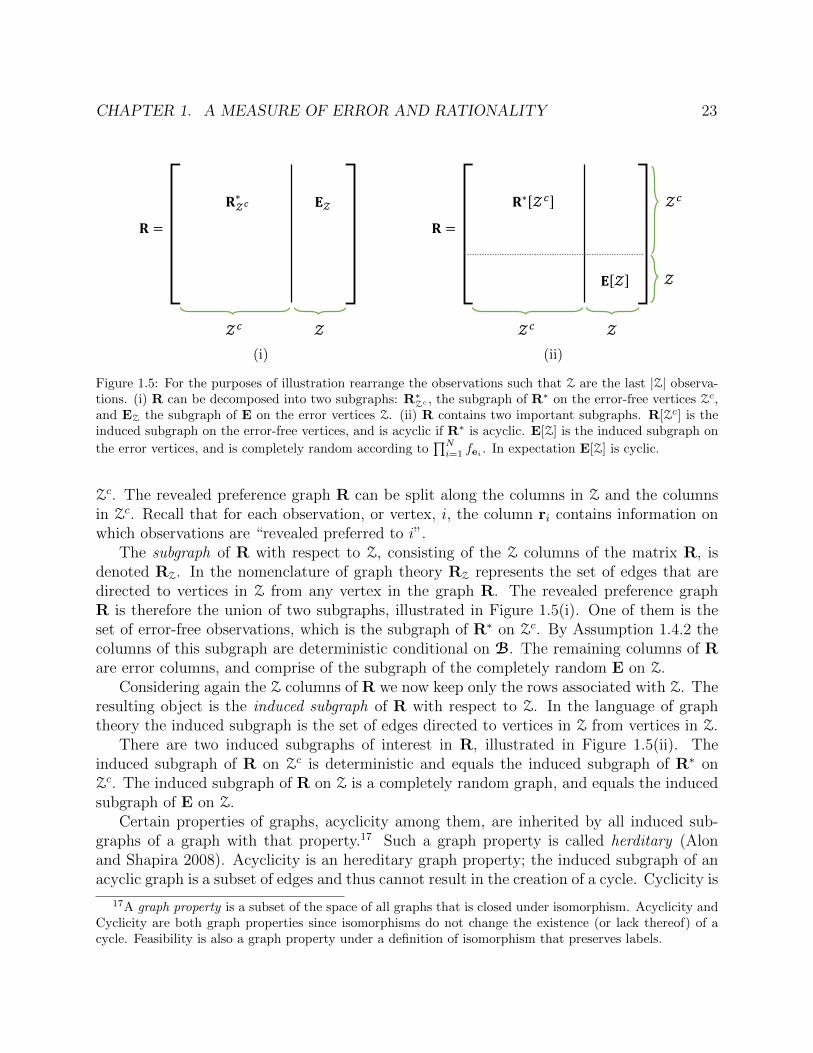
Figure 1.5: For the purposes of illustration rearrange the observations such that Z are the last |Z| observa-tions. (i) R can be decomposed into two subgraphs: R∗Zc , the subgraph of R∗ on the error-free vertices Zc,and EZ the subgraph of E on the error vertices Z. (ii) R contains two important subgraphs. R[Zc] is theinduced subgraph on the error-free vertices, and is acyclic if R∗ is acyclic. E[Z] is the induced subgraph on
the error vertices, and is completely random according to∏N
i=1 fei. In expectation E[Z] is cyclic.
Zc. The revealed preference graph R can be split along the columns in Z and the columnsin Zc. Recall that for each observation, or vertex, i, the column ri contains information onwhich observations are “revealed preferred to i”.
The subgraph of R with respect to Z, consisting of the Z columns of the matrix R, isdenoted RZ. In the nomenclature of graph theory RZ represents the set of edges that aredirected to vertices in Z from any vertex in the graph R. The revealed preference graphR is therefore the union of two subgraphs, illustrated in Figure 1.5(i). One of them is theset of error-free observations, which is the subgraph of R∗ on Zc. By Assumption 1.4.2 thecolumns of this subgraph are deterministic conditional on B. The remaining columns of Rare error columns, and comprise of the subgraph of the completely random E on Z.
Considering again the Z columns of R we now keep only the rows associated with Z. Theresulting object is the induced subgraph of R with respect to Z. In the language of graphtheory the induced subgraph is the set of edges directed to vertices in Z from vertices in Z.
There are two induced subgraphs of interest in R, illustrated in Figure 1.5(ii). Theinduced subgraph of R on Zc is deterministic and equals the induced subgraph of R∗ onZc. The induced subgraph of R on Z is a completely random graph, and equals the inducedsubgraph of E on Z.
Certain properties of graphs, acyclicity among them, are inherited by all induced sub-graphs of a graph with that property.17 Such a graph property is called herditary (Alonand Shapira 2008). Acyclicity is an hereditary graph property; the induced subgraph of anacyclic graph is a subset of edges and thus cannot result in the creation of a cycle. Cyclicity is
17A graph property is a subset of the space of all graphs that is closed under isomorphism. Acyclicity andCyclicity are both graph properties since isomorphisms do not change the existence (or lack thereof) of acycle. Feasibility is also a graph property under a definition of isomorphism that preserves labels.

CHAPTER 1. A MEASURE OF ERROR AND RATIONALITY 24
𝐑 =
𝒵𝑐 𝒵
𝐑∗ 𝒵𝑐
𝐄 𝒵
𝒵𝑐
𝒵
(i)
𝐑 = (𝐼)
(𝐼𝐼)(𝐼𝐼𝐼)
(𝐼𝐼𝐼)
𝑁 − 𝒵 𝒵
𝑁 − 𝒵
𝒵
(ii)
Figure 1.6: R can be decomposed into two induced subgraphs: R[Zc] and E[Z]. The remaining edges aredirected either from Z to Zc or are directed from Zc to Z(ii) These three subsets of edges are labeled (I),(II), (III) and are considered separately as sources for a cycle of length two under the null and under thealternative.
not an hereditary graph property. A subgraph of a cyclic graph does not necessarily includeany edges involved in a cycle, and is potentially acyclic. Feasibility is also an hereditaryproperty since any induced subgraph of a feasible graph is also feasible.
Remark. The set of acyclic feasible graphs A is an hereditary graph property. Hereditaryproperties of the graph R∗ carry over to the induced subgraph of R∗ on Zc, R∗[Zc]. Thuswhenever R∗ is acyclic, the induced subgraph R[Zc] is also acyclic.
Possible Sources of an Observed Cycle
Conditioning on R∗ being acyclic, every cycle involves at least one error column. This resultfollows directly from the remark above. To see why this is the case, consider for now a cycleinvolving two edges, called a 2-cycle or a cycle of length 2.
Recall the two induced subgraphs of R: (I) on Zc and (II) on Z. The remaining edges(III) are directed from Z to Zc or from Zc to Z.18 Figure 1.6(ii) illustrates this division.When R∗ is acyclic, there are no cycles in the induced subgraph R[Zc], (I). In this case, if a2-cycle in R is observed, then there are two possibilities. The first is that the cycle involvestwo errors, and lies in the induced subgraph E[Z], the edges in (II). The second is thatit involves an error-free column and an error column which closes the cycle, in which caseboth edges are in (III). In contrast to the acyclic case, when R∗ is cyclic the cycle mayarise from the induced subgraph R[Zc], the edges (I). These 2-cycles are in addition to thepossible 2-cycles in (II) and (III). Table 1.3 summarizes the above discussion.
18For the reader familiar with graph theory, (III) is the directed cut-set of the cut (Z,Zc).

CHAPTER 1. A MEASURE OF ERROR AND RATIONALITY 25
Possible Source of an Observed 2-cycle
(I) R∗ only (II) E only (III) R∗ and E
R∗ is acyclic X XR∗ is cyclic X X X
Table 1.3: The existence of a 2-cycle in different subsets of the graph depends on the acyclicity of R∗
Recall that by Assumption 1.4.3 each zi is a Bernoulli random variable, so the sets Z andZc are random. Even the cardinality of each set is random: the number of error observations|Z| is distributed as a Binomial random variable with parameters (N, π).
If the probability of an error π is 0, the number of error observations |Z| = 0. In thiscase the graph is deterministic and equal to R∗. Furthermore, an observed cycle indicatesthat R∗ is cyclic (see the first column of Table 1.3). As the error rate π increases towards 1,the number of error observations |Z| increases almost surely to N .19 The distribution of thegraph R thus converges to the probability mass function of E. Determining if R∗ is acyclicor cyclic becomes impossible (see middle column of Table 1.3).
The Expected Number of 2-Cycles
The graph structure of R permits a simple formulation of the expected number of 2-cyclesas a function of R∗ and π. For each R∗, if there are enough observations, π can be estimatedusing the moment condition of the expected number of 2-cycles.20
Let C2(R) be the number of 2-cycles observed in the graph R. The total number of2-cycles in a graph is
C2(R) =∑i<j
I{rji = 1}I{rij = 1}. (1.3)
The summation is over all pairs i < j, because each cycle is only counted once for each pairof observations.
Taking the expected value over this amount, it is helpful to divide the pairs according tothe divisions (I), (II), and (III) in the previous section. As before, Pi (j) is the marginalprobability that a random error column ei indicates that the observed xj is revealed preferred
19The almost sure property arises from a monotone coupling of |Z| under different values of increasing π.20Moments on longer cycles can also be calculated. These are especially useful if the error distribution
has additional parameters such that φ 6= ∅. However, caution should be used because such cycles are rareevents.
CHAPTER 1. A MEASURE OF ERROR AND RATIONALITY 26
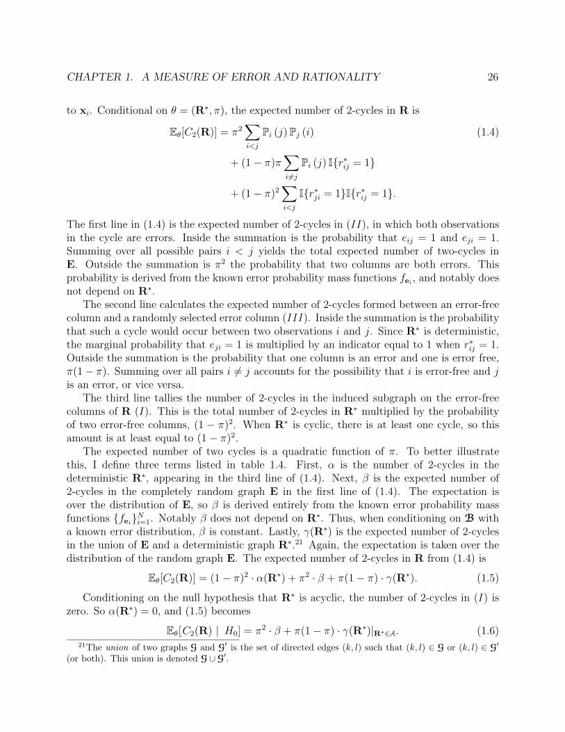
to xi. Conditional on θ = (R∗, π), the expected number of 2-cycles in R is
Eθ[C2(R)] = π2∑i<j
Pi (j)Pj (i) (1.4)
+ (1− π)π∑i 6=j
Pi (j) I{r∗ij = 1}
+ (1− π)2∑i<j
I{r∗ji = 1}I{r∗ij = 1}.
The first line in (1.4) is the expected number of 2-cycles in (II), in which both observationsin the cycle are errors. Inside the summation is the probability that eij = 1 and eji = 1.Summing over all possible pairs i < j yields the total expected number of two-cycles inE. Outside the summation is π2 the probability that two columns are both errors. Thisprobability is derived from the known error probability mass functions fei , and notably doesnot depend on R∗.
The second line calculates the expected number of 2-cycles formed between an error-freecolumn and a randomly selected error column (III). Inside the summation is the probabilitythat such a cycle would occur between two observations i and j. Since R∗ is deterministic,the marginal probability that eji = 1 is multiplied by an indicator equal to 1 when r∗ij = 1.Outside the summation is the probability that one column is an error and one is error free,π(1− π). Summing over all pairs i 6= j accounts for the possibility that i is error-free and jis an error, or vice versa.
The third line tallies the number of 2-cycles in the induced subgraph on the error-freecolumns of R (I). This is the total number of 2-cycles in R∗ multiplied by the probabilityof two error-free columns, (1 − π)2. When R∗ is cyclic, there is at least one cycle, so thisamount is at least equal to (1− π)2.
The expected number of two cycles is a quadratic function of π. To better illustratethis, I define three terms listed in table 1.4. First, α is the number of 2-cycles in thedeterministic R∗, appearing in the third line of (1.4). Next, β is the expected number of2-cycles in the completely random graph E in the first line of (1.4). The expectation isover the distribution of E, so β is derived entirely from the known error probability massfunctions {fei}Ni=1. Notably β does not depend on R∗. Thus, when conditioning on B witha known error distribution, β is constant. Lastly, γ(R∗) is the expected number of 2-cyclesin the union of E and a deterministic graph R∗.21 Again, the expectation is taken over thedistribution of the random graph E. The expected number of 2-cycles in R from (1.4) is
Eθ[C2(R)] = (1− π)2 · α(R∗) + π2 · β + π(1− π) · γ(R∗). (1.5)
Conditioning on the null hypothesis that R∗ is acyclic, the number of 2-cycles in (I) iszero. So α(R∗) = 0, and (1.5) becomes
Eθ[C2(R) | H0] = π2 · β + π(1− π) · γ(R∗)|R∗∈A. (1.6)21The union of two graphs G and G′ is the set of directed edges (k, l) such that (k, l) ∈ G or (k, l) ∈ G′
(or both). This union is denoted G ∪ G′.
CHAPTER 1. A MEASURE OF ERROR AND RATIONALITY 27
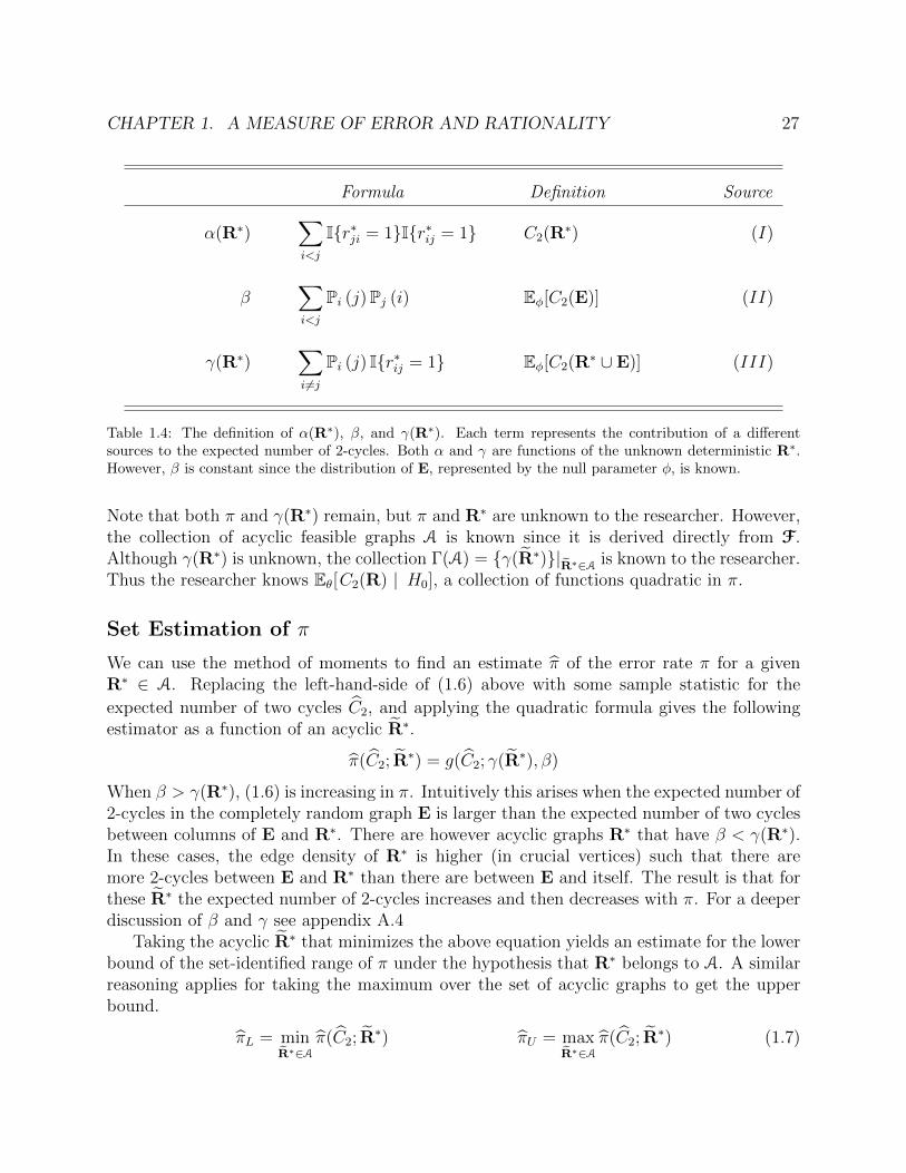
Formula Definition Source
α(R∗)∑i<j
I{r∗ji = 1}I{r∗ij = 1} C2(R∗) (I)
β∑i<j
Pi (j)Pj (i) Eφ[C2(E)] (II)
γ(R∗)∑i 6=j
Pi (j) I{r∗ij = 1} Eφ[C2(R∗ ∪ E)] (III)
Table 1.4: The definition of α(R∗), β, and γ(R∗). Each term represents the contribution of a differentsources to the expected number of 2-cycles. Both α and γ are functions of the unknown deterministic R∗.However, β is constant since the distribution of E, represented by the null parameter φ, is known.
Note that both π and γ(R∗) remain, but π and R∗ are unknown to the researcher. However,the collection of acyclic feasible graphs A is known since it is derived directly from F.Although γ(R∗) is unknown, the collection Γ(A) = {γ(R∗)}|R∗∈A is known to the researcher.Thus the researcher knows Eθ[C2(R) | H0], a collection of functions quadratic in π.
Set Estimation of π
We can use the method of moments to find an estimate π of the error rate π for a givenR∗ ∈ A. Replacing the left-hand-side of (1.6) above with some sample statistic for the
expected number of two cycles C2, and applying the quadratic formula gives the followingestimator as a function of an acyclic R∗.
π(C2; R∗) = g(C2; γ(R∗), β)
When β > γ(R∗), (1.6) is increasing in π. Intuitively this arises when the expected number of2-cycles in the completely random graph E is larger than the expected number of two cyclesbetween columns of E and R∗. There are however acyclic graphs R∗ that have β < γ(R∗).In these cases, the edge density of R∗ is higher (in crucial vertices) such that there aremore 2-cycles between E and R∗ than there are between E and itself. The result is that forthese R∗ the expected number of 2-cycles increases and then decreases with π. For a deeperdiscussion of β and γ see appendix A.4
Taking the acyclic R∗ that minimizes the above equation yields an estimate for the lowerbound of the set-identified range of π under the hypothesis that R∗ belongs to A. A similarreasoning applies for taking the maximum over the set of acyclic graphs to get the upperbound.
πL = minR∗∈A
π(C2; R∗) πU = max
R∗∈Aπ(C2; R
∗) (1.7)

CHAPTER 1. A MEASURE OF ERROR AND RATIONALITY 28
Minimizing the function g amounts to finding the R∗ that maximizes the function γ(R∗).The reverse is true for finding the upper bound.
To estimate the expected number of two cycles from the observed sample the graphstructure of R is again leveraged. Consider the induced subgraph of R on some randomlydrawn subset of observations W ⊆ V. The proposed estimator of C2(R) is the average of thenumber of 2-cycles on an induced subgraph over repeated samples. As long as W is drawnindependently of R, the law of iterated expectations yields
Eθ[C2(R)
cN
]= EW
[Eθ[C2(R[W])
c|W|
∣∣∣∣ W]].The outer expectation EW is taken over the sample W. Both the left and right side arenormalized by a constant cn = n(n− 1)/2. The number of 2-cycles is a function of the sizeN × N of R. So the expectation over a subgraph is equal only when normalized by themaximum number of 2-cycles cn.
Consider a sequence of W = {W1, ...WT} of random samples without replacement of thevertices V. Let each subsample Wt be the same size |Wt| = M .22 Each subsample of size Mhas the same probability of being drawn. Thus the sample statistic is
C2 =1
T
∑W
C2(R[Wt])
cM. (1.8)
The estimator in (1.8) above yields a lower and upper bound on the error rate π, as outlinedin (1.7).
1.6 Simulation Results
Four simulations demonstrate the use of this method. The first simulation demonstratesthat the distribution of C2(R) is centered at the expected value under the true R∗ and π.The second simulation demonstrates the subsampling approach when only one observationof R is given. The third simulation explores the minimum γ values as N increases. If the R∗
that minimizes γ at smaller N is an induced subgraph of the minimizing R∗, then there is a“stable” minimum γ, which allows for a subsampling on the right-hand-side of (1.6). This isdesirable because finding the global minimum of γ on all acyclic graphs is computationallyintensive (increasing exponentially in N2). The fourth simulation compares the estimate ofπ to existing indices such as Afriat’s CCEI and Varian’s Index for select choice data sets.
Results are presented for the first simulation. As of the writing of this draft, resultsare underway but not yet presentable for simulations 2, 3, and 4. The simulations wereconducted in R programming language. Code will be available in the online appendix uponpublication.
22Following Romano and Shaikh (2008) it may be desirable for M to be some function of N such thatMN ¡ N and MN
N → 0.
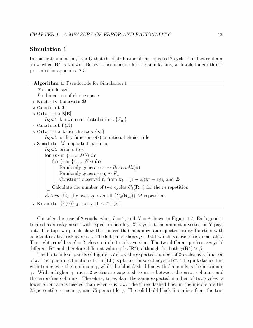
CHAPTER 1. A MEASURE OF ERROR AND RATIONALITY 29
Simulation 1
In this first simulation, I verify that the distribution of the expected 2-cycles is in fact centeredon π when R∗ is known. Below is pseudocode for the simulations, a detailed algorithm ispresented in appendix A.5.
Algorithm 1: Pseudocode for Simulation 1
N : sample sizeL : dimension of choice space
1 Randomly Generate B
2 Construct F
3 Calculate E[E]Input: known error distributions {Fui
}4 Construct Γ(A)5 Calculate true choices {x∗i }
Input: utility function u(·) or rational choice rule6 Simulate M repeated samples
Input: error rate πfor (m in {1, ...,M}) do
for (i in {1, ..., N}) doRandomly generate zi ∼ Bernoulli(π)Randomly generate ui ∼ Fui
Construct observed ri from xi = (1− zi)x∗i + ziui and B
Calculate the number of two cycles C2(Rm) for the m repetition
Return: C2, the average over all {C2(Rm)} M repetitions
7 Estimate {π(γ)}|A for all γ ∈ Γ(A)
Consider the case of 2 goods, when L = 2, and N = 8 shown in Figure 1.7. Each good istreated as a risky asset; with equal probability, X pays out the amount invested or Y paysout. The top two panels show the choices that maximize an expected utility function withconstant relative risk aversion. The left panel shows ρ = 0.01 which is close to risk neutrality.The right panel has ρ′ = 2, close to infinite risk aversion. The two different preferences yielddifferent R∗ and therefore different values of γ(R∗), although for both γ(R∗) > β.
The bottom four panels of Figure 1.7 show the expected number of 2-cycles as a functionof π. The quadratic function of π in (1.6) is plotted for select acyclic R∗. The pink dashed linewith triangles is the minimum γ, while the blue dashed line with diamonds is the maximumγ. With a higher γ, more 2-cycles are expected to arise between the error columns andthe error-free columns. Therefore, to explain the same expected number of two cycles, alower error rate is needed than when γ is low. The three dashed lines in the middle are the25-percentile γ, mean γ, and 75-percentile γ. The solid bold black line arises from the true
CHAPTER 1. A MEASURE OF ERROR AND RATIONALITY 30
γ(R∗) generated by x∗i . Since γ(R∗) > β, the quadratic functions are concave, while thecurves with γ < β are convex.
Simulation 1 is conducted over M = 10, 000 repetitions. The true π is indicated by thestraight vertical line, while the estimate for C2 from the averaged repeated samples is markedby the horizontal line. Results are shown for both π = 0.2 and π = 0.5. As desired, the twolines cross each other close to the solid black line. This means that as expected, the inversionof (1.6) results in a point estimate of π. Since R∗ is not known, we use the set-estimationwhich is indicated by the values of π where the horizontal line crosses the minimum γ(R∗)and the maximum γ(R∗). This is the identified set estimate of π. We could use the range ofvalues, or we could consider the finite set of values within, which as demonstrated with theremaining three lines, is concentrated close to the line where γ = β.
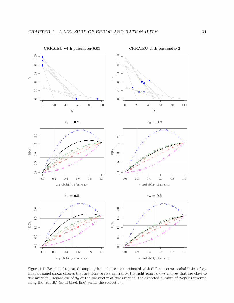
CHAPTER 1. A MEASURE OF ERROR AND RATIONALITY 31
0 20 40 60 80 100
020
4060
8010
0
CRRA.EU with parameter 0.01
X
Y
0 20 40 60 80 100
020
4060
8010
0
CRRA.EU with parameter 2
XY
0.0 0.2 0.4 0.6 0.8 1.0
0.0
0.5
1.0
1.5
2.0
π0 = 0.2
π probability of an error
E[C
2]
0.0 0.2 0.4 0.6 0.8 1.0
0.0
0.5
1.0
1.5
2.0
π0 = 0.2
π probability of an error
E[C
2]
0.0 0.2 0.4 0.6 0.8 1.0
0.0
0.5
1.0
1.5
2.0
π0 = 0.5
π probability of an error
E[C
2]
0.0 0.2 0.4 0.6 0.8 1.0
0.0
0.5
1.0
1.5
2.0
π0 = 0.5
π probability of an error
E[C
2]
Figure 1.7: Results of repeated sampling from choices contaminated with different error probabilities of π0.The left panel shows choices that are close to risk neutrality, the right panel shows choices that are close torisk aversion. Regardless of π0 or the parameter of risk aversion, the expected number of 2-cycles invertedalong the true R∗ (solid black line) yields the correct π0.
CHAPTER 1. A MEASURE OF ERROR AND RATIONALITY 32
1.7 Directions of Future Work
In the short-term there are a few directions of future research. An application of this methodto choice data elicited in the lab is in progress, with data from Choi, Fisman, Gale, andKariv (2007a). In addition to comparing minimum estimates of π to existing indices, thisempirical application will provide guidance on how to decide data quality. A formalizationof the intuition in appendix A.4 is also underway, with the goal of providing guidance inexperimental design. An exploration of the use of subsampling to build standard errors onthe set estimate of π is also in progress (Romano and Shaikh 2008). Lastly, the recent versionof Nishimura, Ok, and Quah (2016) opens up the possibility to applying this approach tochoice data in discrete settings.
In the long-term there are many directions of future research that will yield fruitful resultsto both practitioners and theorists. These largely fall into the three broad categories thatthis research touches upon: experimental & behavioral economics, microeconomics theory,and econometrics.
An obvious follow-up to this article involves recoverability of preferences. It is possibleto apply the estimator of π to more specific subsets of R∗ (see Polisson, Quah, and Renou(2015) for an example of such nested tests). This can connect to recent work by Halevy,Persitz, and Zrill (2015) on parametric recoverability of preferences.
Another direction of research is an application of the random revealed preference relationto state dependent preferences. In situations where rationality is conditional on an observablevariable that is thought to identify different states, it may be possible to identify the differentstates, holding π fixed. This will add to a budding literature on nonparametric analysis ofstate-dependent preferences (for the most recent citations see Crawford and Pendakur (2012)and Liang (2016)).
Lastly, there are numerous avenues of theoretical research in the study of random revealedpreferences that can be pursued. A deeper exploration of various properties of R and itsdistribution is certainly warranted. A search for an ancillary statistic or a proof of non-existence in the spirit of Pena et al. (1992) is also necessary. Asymptotic analysis of thedistribution of R as the number of observations N →∞ is an especially ripe field (see Reny(2015) for an idea of how to extend the microeconomic theory alongside the econometrics).Characterizing the distribution of R, while not straightforward, should be possible. Relatingthe limiting object of R to the utility function means that π can differentiate measurementfrom model error.
33
Chapter 2
The external validity of in-lab rationalbehavior
Introduction
Past results from lab experiments have shown that individual choices over risky assets arefor the most part rational, meaning that decisions are consistent with utility maximization(Choi, Fisman, Gale, and Kariv 2007a). Yet the external validity of observed rationality in-lab is called into question by the controlled environment and short time frame of experimentsconducted in the lab. To address this concern, we conduct a lab-in-field study over a fiveday period using an experiment interface installed directly on participants’ smartphones.
Individual rationality is a linchpin assumption in almost all economic theories. Choicesthat are rational can be modeled as if they are the result of utility maximization. Rationalchoices at their heart imply that an individual has some consistent preference ordering overany set of alternatives. The existence of such a preference ordering allows economists to con-duct inference on choices at the individual level, and to aggregate welfare across a populationso as to measure social welfare 1. Establishing rationality in the face of risky alternatives isespecially important because risk pervades numerous facets of life- from investment decisionsto health care options to career choice.
To test if an individual’s choices over risky assets are rational, we elicit a sequenceof decisions from participants using a well established graphical interface (Choi, Fisman,Gale, and Kariv 2007b). The graphical interface yields a rich dataset that lends itself tononparametric tests of rationality. In the lab the choices are presented on a computermonitor, in quick succession over the course of an hour. For the lab-in-field design, thedecision problems are presented over the course of five days through a custom application
1Individual welfare cannot be compared across the population due to the ordinal nature of preferences.To measure social welfare, economists quantify the relative preferences of an individual into money, whichis then be aggregated across a individuals. If individual choices are not rational, then this quantification ofwelfare is meaningless.
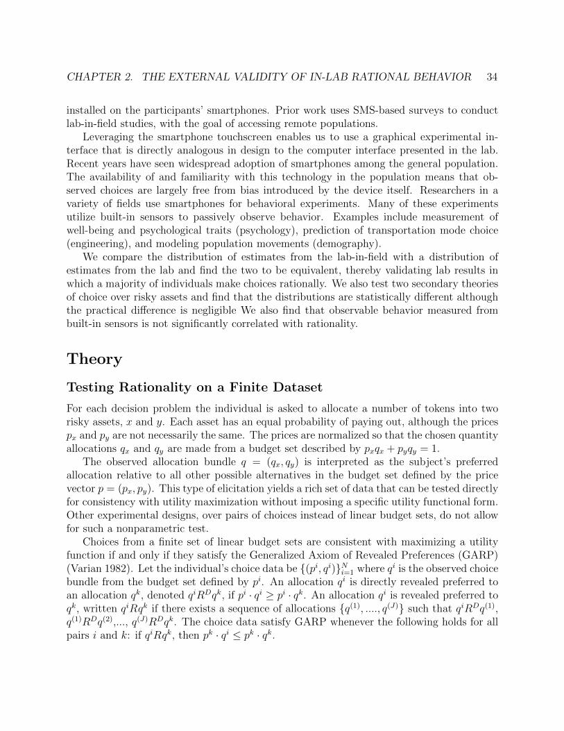
CHAPTER 2. THE EXTERNAL VALIDITY OF IN-LAB RATIONAL BEHAVIOR 34
installed on the participants’ smartphones. Prior work uses SMS-based surveys to conductlab-in-field studies, with the goal of accessing remote populations.
Leveraging the smartphone touchscreen enables us to use a graphical experimental in-terface that is directly analogous in design to the computer interface presented in the lab.Recent years have seen widespread adoption of smartphones among the general population.The availability of and familiarity with this technology in the population means that ob-served choices are largely free from bias introduced by the device itself. Researchers in avariety of fields use smartphones for behavioral experiments. Many of these experimentsutilize built-in sensors to passively observe behavior. Examples include measurement ofwell-being and psychological traits (psychology), prediction of transportation mode choice(engineering), and modeling population movements (demography).
We compare the distribution of estimates from the lab-in-field with a distribution ofestimates from the lab and find the two to be equivalent, thereby validating lab results inwhich a majority of individuals make choices rationally. We also test two secondary theoriesof choice over risky assets and find that the distributions are statistically different althoughthe practical difference is negligible We also find that observable behavior measured frombuilt-in sensors is not significantly correlated with rationality.
Theory
Testing Rationality on a Finite Dataset
For each decision problem the individual is asked to allocate a number of tokens into tworisky assets, x and y. Each asset has an equal probability of paying out, although the pricespx and py are not necessarily the same. The prices are normalized so that the chosen quantityallocations qx and qy are made from a budget set described by pxqx + pyqy = 1.
The observed allocation bundle q = (qx, qy) is interpreted as the subject’s preferredallocation relative to all other possible alternatives in the budget set defined by the pricevector p = (px, py). This type of elicitation yields a rich set of data that can be tested directlyfor consistency with utility maximization without imposing a specific utility functional form.Other experimental designs, over pairs of choices instead of linear budget sets, do not allowfor such a nonparametric test.
Choices from a finite set of linear budget sets are consistent with maximizing a utilityfunction if and only if they satisfy the Generalized Axiom of Revealed Preferences (GARP)(Varian 1982). Let the individual’s choice data be {(pi, qi)}Ni=1 where qi is the observed choicebundle from the budget set defined by pi. An allocation qi is directly revealed preferred toan allocation qk, denoted qiRDqk, if pi · qi ≥ pi · qk. An allocation qi is revealed preferred toqk, written qiRqk if there exists a sequence of allocations {q(1), ...., q(J)} such that qiRDq(1),q(1)RDq(2),..., q(J)RDqk. The choice data satisfy GARP whenever the following holds for allpairs i and k: if qiRqk, then pk · qi ≤ pk · qk.

CHAPTER 2. THE EXTERNAL VALIDITY OF IN-LAB RATIONAL BEHAVIOR 35
GARP provides a direct, but binary, test of rationality- either the choice data satisfyGARP or they do not. Various goodness of fit measures have been developed to measurehow “far” from rationality a given dataset is from satisfying GARP (Halevy, Persitz, andZrill 2015). The most common measure is Afriat’s Critical Cost Efficiency Index (CCEI)which measures distance as a fraction of the prices. Consider the budget line defined asep · q = 1 where e is some number between 0 and 1. There exists some e such that thehypothetical dataset {(epi, qi)}Ni=1 satisfies GARP. Afriat’s CCEI solves a system of linearinequalities to find the maximum value of e for which the altered data satisfy GARP (Afriat1972). The closer e is to 1, the closer the dataset is to being completely rational.
Testing Expected Utility on a Finite Dataset
In addition to rationality it is possible to test hypotheses more specific to the risk environ-ment. We preset two such tests due to Polisson, Quah, and Renou (2015).
When modeling choices over risky assets, it is reasonable to expect that an individual willnot choose an option that is stochastically dominated by another available alternative. Abundle q stochastically dominates another bundle q′ in the first order if the expected payoutfrom q is higher than the expected payout from q′, which in the case of equal probabilitiesfor x and y means that 0.5qx + 0.5qy ≥ 0.5q′x + 0.5q′y. A choice dataset {(pi, qi)}Ni=1 satisfiesfirst order stochastic dominance (FOSD) if the inequality above holds for every i with q = qi
and q′ is any choice bundle in the budget set defined by pi. Similar to Afriat’s CCEI it ispossible to measure the goodness of fit of FOSD by finding the maximum e such that thedataset {(epi, qi)}Ni=1 is satisfies FOSD. This value of e is usually not the same as Afriat’sCCEI, and is called the FOSD CCEI.
The most common utility function used to model choices over risky assets is ExpectedUtility (EU). The expected utility from a bundle q with equal probabilities over x and y isdefined as EU(q;u) = 0.5u(qx) + 0.5u(qy), where u is a continuous increasing function. Thefunction u represents an individual’s utility over money. The observed choices are consistentwith expected utility if there exists a function u such that for every i, EU(qi;u) ≥ EU(q;u)for any bundle q affordable under pi, meaning that pi · q ≤ 1.
This condition is equivalent to finding a function u such that for every observation i, theexpected utility at the chosen allocation qi is at least as much as the expected utility at anyother affordable (and unchosen) allocation. To check the existence of such a utility functionone can solve for a finite set of utility values such that a certain set of linear inequalitieshold. Again, by finding the the maximum e such that the dataset {(epi, qi)}Ni=1 is consistentwith expected utility, we can measure the goodness of fit of the expected utility hypothesis.Again, when e is 1, the dataset is consistent with expected utility. We call this value of e,EU CCEI.
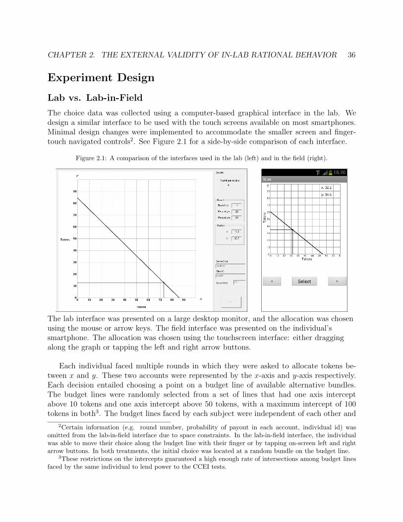
CHAPTER 2. THE EXTERNAL VALIDITY OF IN-LAB RATIONAL BEHAVIOR 36
Experiment Design
Lab vs. Lab-in-Field
The choice data was collected using a computer-based graphical interface in the lab. Wedesign a similar interface to be used with the touch screens available on most smartphones.Minimal design changes were implemented to accommodate the smaller screen and finger-touch navigated controls2. See Figure 2.1 for a side-by-side comparison of each interface.
Figure 2.1: A comparison of the interfaces used in the lab (left) and in the field (right).
The lab interface was presented on a large desktop monitor, and the allocation was chosenusing the mouse or arrow keys. The field interface was presented on the individual’ssmartphone. The allocation was chosen using the touchscreen interface: either draggingalong the graph or tapping the left and right arrow buttons.
Each individual faced multiple rounds in which they were asked to allocate tokens be-tween x and y. These two accounts were represented by the x-axis and y-axis respectively.Each decision entailed choosing a point on a budget line of available alternative bundles.The budget lines were randomly selected from a set of lines that had one axis interceptabove 10 tokens and one axis intercept above 50 tokens, with a maximum intercept of 100tokens in both3. The budget lines faced by each subject were independent of each other and
2Certain information (e.g. round number, probability of payout in each account, individual id) wasomitted from the lab-in-field interface due to space constraints. In the lab-in-field interface, the individualwas able to move their choice along the budget line with their finger or by tapping on-screen left and rightarrow buttons. In both treatments, the initial choice was located at a random bundle on the budget line.
3These restrictions on the intercepts guaranteed a high enough rate of intersections among budget linesfaced by the same individual to lend power to the CCEI tests.

CHAPTER 2. THE EXTERNAL VALIDITY OF IN-LAB RATIONAL BEHAVIOR 37
independent from those faced by other subjects. The resolution on the choice space was inincrements of 0.2 tokens in the lab and increments of 0.01 tokens in the lab-in-field.
Data
For the lab treatment we use observations from two studies (Choi, Fisman, Gale, and Kariv2007a; Cappelen, Kariv, Sorensen, and Tungodden 2015). We use all 43 participants inthe symmetric treatment from Choi et al. (2007a) and all 126 US subjects from Cappelenet al. (2015) for a total of 173 subjects recruited from UC Berkeley students and staff.Both studies were conducted using the computer lab at UC Berkeley’s Experimental SocialScience Laboratory (XLab). The experimental procedure was identical in both studies:subjects read the instructions, after which an experimenter read the instructions out loud.The subsequent experimental sessions lasted about 1.5 hours and consisted of 50 decisionproblems. Decisions were made over tokens, where every token was worth $0.50 dollars. Atthe end of the experiment one of the fifty rounds and one of the goods (x or y) were randomlyselected to pay out to the participant. Lab participants earned a $5 “show-up” payment andthe payouts from the decision problems averaged $19.
The lab-in-field experiment was conducted over a 5 day period with 127 participants.A total of 160 participants were recruited, however 34 subjects were excluded from thefinal analysis due to technical issues (25) and attrition (8). The lab-in-field experiment wasconducted remotely, where the consent form, instructions, and smartphone app were sentto participants over email. Each participant installed a custom-built “native” applicationonto their smartphone4. The opening screen showed the instructions, which were identicalto those sent via email to participants. A total of 50 decision problems were “pushed” tothe participant’s phone at random times between 9:00 AM and 9:00 PM on Monday throughFriday of the experiment. A notification would appear on the subjects’ phone, informingthem that a decision problem was available. We allowed for first-in first-out queuing of upto 3 decision problems, after which a decision problem would be marked as unanswered anda choice of (0,0) automatically entered5. Again, one of the fifty rounds and either x or ywere randomly chosen as the participant’s payout. There was no “show-up” payment and onaverage participants earned $17 in the lab-in-field experiments; not included in this averageare the 46 participants who earned $0 because of missing responses for the selected round.As in the lab treatment, subjects were not informed of their payout until the end of theexperiment.
4For technical reasons we restricted our study to Android phone users. More specifically: Native appsare written in different languages depending on the operating system of the phone (Apple iOS, Android,Windows). The app was developed for Android phones and would have been prohibitively difficult to buildfor other operating systems.
5The response rate in the lab-in-field treatment ranged from 50% - 100%. We excluded 8 subjects fromthe study with response rates below 50% which we attribute to attrition from the study. The averageresponse rate was 89.4%, median was 94%. The first and third quartile response rates were 85% and 98%respectively.
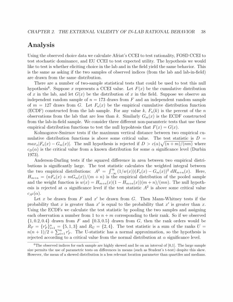
CHAPTER 2. THE EXTERNAL VALIDITY OF IN-LAB RATIONAL BEHAVIOR 38
Analysis
Using the observed choice data we calculate Afriat’s CCEI to test rationality, FOSD CCEI totest stochastic dominance, and EU CCEI to test expected utility. The hypothesis we wouldlike to test is whether eliciting choice in the lab and in the field yield the same behavior. Thisis the same as asking if the two samples of observed indices (from the lab and lab-in-field)are drawn from the same distribution.
There are a number of two-sample statistical tests that could be used to test this nullhypothesis6. Suppose x represents a CCEI value. Let F (x) be the cumulative distributionof x in the lab, and let G(x) be the distribution of x in the field. Suppose we observe anindependent random sample of n = 173 draws from F and an independent random sampleof m = 127 draws from G. Let Fn(x) be the empirical cumulative distribution function(ECDF) constructed from the lab sample. For any value k, Fn(k) is the percent of the nobservations from the lab that are less than k. Similarly Gm(x) is the ECDF constructedfrom the lab-in-field sample. We consider three different non-paramteric tests that use theseempirical distribution functions to test the null hypohtesis that F (x) = G(x).
Kolmogorov-Smirnov tests if the maximum vertical distance between two empirical cu-mulative distribution functions is above some critical value. The test statistic is D =maxx|Fn(x)−Gm(x)|. The null hypothesis is rejected if D > c(α)
√(n+m)/(nm) where
cD(α) is the critical value from a known distribution for some α significance level (Durbin1973).
Anderson-Darling tests if the squared difference in area between two empirical distri-butions is significantly large. The test statistic calculates the weighted integral betweenthe two empirical distributions: A2 =
∫∞−∞ (1/w(x))(Fn(x)−Gm(x))2 dHm+n(x). Here,
Hm+n = (nFn(x) + mGm(x))/(m + n) is the empirical distribution of the pooled sampleand the weight function is w(x) = Hm+n(x)(1−Hm+n(x))(m + n)/(mn). The null hypoth-esis is rejected at α significance level if the test statistic A2 is above some critical valuecA2(α).
Let x be drawn from F and x′ be drawn from G. Then Mann-Whitney tests if theprobability that x is greater than x′ is equal to the probability that x′ is greater than x.Using the ECDFs we calculate the test statistic by pooling the two samples and assigningeach observation a number from 1 to n + m corresponding to their rank. So if we observed{1, 0.2, 0.4} drawn from F and {0.3, 0.5} drawn from G, then the rank orders would beRF = {riF}ni=1 = {5, 1, 3} and RG = {2, 4}. The test statistic is a sum of the ranks U =n(n + 1)/2 +
∑ni=1 r
iF . The U-statistic has a normal approximation, so the hypothesis is
rejected according to a critical value from the normal distribution at α significance level.
6The observed indices for each sample are highly skewed and lie on an interval of [0,1]. The large samplesize permits the use of parametric tests on differences in means (such as Student’s t-test) despite this skew.However, the mean of a skewed distribution is a less relevant location parameter than quartiles and medians.
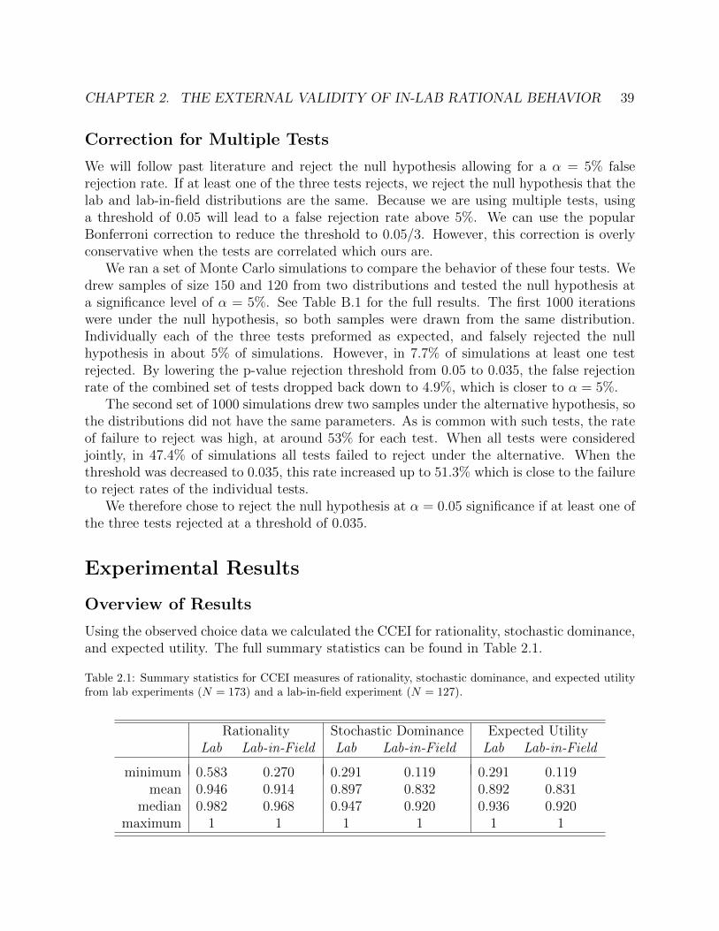
CHAPTER 2. THE EXTERNAL VALIDITY OF IN-LAB RATIONAL BEHAVIOR 39
Correction for Multiple Tests
We will follow past literature and reject the null hypothesis allowing for a α = 5% falserejection rate. If at least one of the three tests rejects, we reject the null hypothesis that thelab and lab-in-field distributions are the same. Because we are using multiple tests, usinga threshold of 0.05 will lead to a false rejection rate above 5%. We can use the popularBonferroni correction to reduce the threshold to 0.05/3. However, this correction is overlyconservative when the tests are correlated which ours are.
We ran a set of Monte Carlo simulations to compare the behavior of these four tests. Wedrew samples of size 150 and 120 from two distributions and tested the null hypothesis ata significance level of α = 5%. See Table B.1 for the full results. The first 1000 iterationswere under the null hypothesis, so both samples were drawn from the same distribution.Individually each of the three tests preformed as expected, and falsely rejected the nullhypothesis in about 5% of simulations. However, in 7.7% of simulations at least one testrejected. By lowering the p-value rejection threshold from 0.05 to 0.035, the false rejectionrate of the combined set of tests dropped back down to 4.9%, which is closer to α = 5%.
The second set of 1000 simulations drew two samples under the alternative hypothesis, sothe distributions did not have the same parameters. As is common with such tests, the rateof failure to reject was high, at around 53% for each test. When all tests were consideredjointly, in 47.4% of simulations all tests failed to reject under the alternative. When thethreshold was decreased to 0.035, this rate increased up to 51.3% which is close to the failureto reject rates of the individual tests.
We therefore chose to reject the null hypothesis at α = 0.05 significance if at least one ofthe three tests rejected at a threshold of 0.035.
Experimental Results
Overview of Results
Using the observed choice data we calculated the CCEI for rationality, stochastic dominance,and expected utility. The full summary statistics can be found in Table 2.1.
Table 2.1: Summary statistics for CCEI measures of rationality, stochastic dominance, and expected utilityfrom lab experiments (N = 173) and a lab-in-field experiment (N = 127).
Rationality Stochastic Dominance Expected UtilityLab Lab-in-Field Lab Lab-in-Field Lab Lab-in-Field
minimum 0.583 0.270 0.291 0.119 0.291 0.119mean 0.946 0.914 0.897 0.832 0.892 0.831
median 0.982 0.968 0.947 0.920 0.936 0.920maximum 1 1 1 1 1 1

CHAPTER 2. THE EXTERNAL VALIDITY OF IN-LAB RATIONAL BEHAVIOR 40
We conduct the three nonparametric tests and find that the null hypothesis cannot berejected for rationality, but it can be rejected for stochastic dominance and expected utilityat statistical significance of α = 5%. For an overview of the test results see Table 2.2.
More specifically, for rationality, we found that Kolmogorov-Smirnov (D = 0.16 withp-value = 0.0495), Man-Whitney (U = 11850, p = 0.24), and Anderson Darling (A2 = 1.76,p = 0.061) all failed to reject at α = 5% using the corrected threshold of 0.035. Since noneof the individual tests reject, we do not reject the hypothesis that rationality in the lab andin the field is equivalent.
For stochastic dominance, Kolmogorov-Smirnov (D = 0.15, p = 0.065) and Man-Whitney(U = 12213.5, p = 0.098) both fail to reject, although Anderson-Darling (A2 = 3.54, p =0.012) does reject using the 0.035 threshold. Since at least one of the tests rejected, we rejectthe null hypothesis that stochastic dominance is equivalent in the lab and in the field, withstatistical significance of α = 5%.
Turning our attention to expected utility, we find that Kolmogorov-Smirnov (D = 0.15,p = 0.082) and Man-Whitney (U = 11882.5,p = 0.23) both fail to reject, although Anderson-Darling (A2 = 3.13, p = 0.018) does reject using the threshold of 0.035. Again, since at leastone of the tests rejected, we reject the null hypothesis that expected utility is the same inthe lab and in the field, with statistical significance of α = 5%.
Discussion of results
Figure 2.2 shows the lab and lab-in-field ECDF’s for Afriat’s CCEI, FOSD CCEI, and EUCCEI. Visual inspection shows that the three measures generally behave similarly. In fact,had we used a significance level of α = 10%, we would have rejected the null hypothesis forrationality as well as the null for stochastic dominance and expected utility. See Table B.2in Appendix B.1 for results from the Monte Carlo simulations under α = 10%, where thecorrected threshold is shown to be 0.07.
Further visual inspection of the ECDF’s sheds insight on the results in 2.2. First, forall three CCEI scores, the Mann-Whitney test does not reject the null at 5% or 10% α.Visually the two ECDFs look to be of the same shape. When the two distributions arethe same shape, the Mann-Whitney test can be interpreted as a test of the medians. Wecan therefore conclude that for all three measures, the medians of the lab and lab-in-fielddistributions are likely not too different. Note that the medians of the three CCEIs are allabove 0.92.
A second thing to notice that the Anderson-Darling test is the only test to reject atα = 5% and is also the only test to reject the null for all three CCEI’s at α = 10%. Anderson-Darling measures a weighted squared area between the two ECDF’s. It is therefore morelikely to pick up differences in distributions at the tail (as opposed to the median). Thus,we can infer that the lab-in-field and lab distributions are likely different in the lower tail.
Putting these two insights together we can conclude that people who are irrational in thelab are likely to behave “more” irrationally in the field. So the lab environment may temperthe magnitude of the irrationality. However, people in the lab who behave rationally enough

CHAPTER 2. THE EXTERNAL VALIDITY OF IN-LAB RATIONAL BEHAVIOR 41
Figure 2.2: Empirical distributions of CCEI measures of rationality, stochastic dominance, and expectedutility from experiments in the lab-in-field (N = 127) and lab (N = 173).
to garner a CCEI of 0.92 or above, will generally still be rational in the field. This sameinsight applies to stochastic dominance and expected utility.

CHAPTER 2. THE EXTERNAL VALIDITY OF IN-LAB RATIONAL BEHAVIOR 42
Table 2.2: Main results from two-sided tests at α = 5% statistical significance with multiple-testing correctedthreshold of 0.035.
Rationality Stochastic Dominance Expected Utility
Kolmogorov- 0.16 (0.0495). 0.15 (0.0651). 0.15 (0.0818)Smirnov
Mann- 11850 (0.2429) 12213.5 (0.0982) 11882.5 (0.2272)Whitney
Anderson- 1.76 (0.0605). 3.54 (0.0124)* 3.13 (0.0175)*Darling
At least onetest rejects? No Yes Yes
(α = 5%)
Note: If the p-value is below the corrected threshold of 0.035 for α = 5% it is marked ’*’, ifit is below the corrected threshold of 0.07 for α = 10% it is marked ’.’. Each column tests adifferent measure of CCEI. Values reported are the test statistic and in parentheses thep-value. The bottom row indicates whether at least one of the tests rejects.
43
Bibliography
Afriat, S. N. (1967). The Construction of Utility Functions from Expenditure Data. Inter-national Economic Review 8 (1), 67–77.
Afriat, S. N. (1972). Efficiency Estimation of Production Functions. International EconomicReview 13 (3), 568–598.
Alon, N. and A. Shapira (2008). A Characterization of the (Natural) Graph PropertiesTestable with One-Sided Error. SIAM Journal on Computing 37 (6), 1703–1727.
Andreoni, J., B. J. Gillen, and W. T. Harbaugh (2013). The Power of Revealed PreferenceTests: Ex-Post Evaluation of Experimental Design.
Blundell, R. W., M. Browning, and I. A. Crawford (2003). Nonparametric Engel Curves andRevealed Preference. Econometrica 71 (1), 205–240.
Blundell, R. W., M. Browning, and I. A. Crawford (2008). Best Nonparametric Bounds onDemand Responses. Econometrica 76 (6), 1227–1262.
Boccardi, M. J. (2016). Predictive Ability and the Fit-Power Trade-Off in Theories ofConsumer Behavior.
Bronars, S. G. (1987). the Power of Nonparametric Tests of Preference Maximization. Econo-metrica 55 (3), 693–698.
Cappelen, A. W., S. Kariv, E. O. Sorensen, and B. Tungodden (2015). Is There a Develop-ment Gap in Rationality?
Chambers, C. P. and F. Echenique (2016). Revealed Preference Theory. Cambridge Univer-sity Press.
Choi, S., R. Fisman, D. Gale, and S. Kariv (2007a). Consistency and Heterogeneity ofIndividual Behavior under Uncertainty. American Economic Review 97 (5), 1921–1938.
Choi, S., R. Fisman, D. Gale, and S. Kariv (2007b). Revealing Preferences Graphically:An Old Method Gets a New Tool Kit. American Economic Review, Papers & Proceed-ings 97 (2), 153–158.

BIBLIOGRAPHY 44
Crawford, I. A. and K. Pendakur (2012). Appendix: How Many Types Are There? TheEconomic Journal 123 (567), 77–95.
de Berg, M., O. Cheong, M. van Kreveld, and M. Overmars (2008). Line Segment Intersec-tion. In Computational Geometry Algorithms and Applications, pp. 19–43. Springer-Verlag.
Deb, R. and M. M. Pai (2014). The geometry of revealed preference. Journal of MathematicalEconomics 50 (1), 203–207.
Diewert, W. E. (1973). Afriat and Revealed Preference Theory. Review of Economic Stud-ies 40 (3), 419–425.
Echenique, F., S. Lee, and M. Shum (2011). The Money Pump as a Measure of RevealedPreference Violations. Journal of Political Economy 119 (6), 1201–1223.
Epstein, L. G. and A. J. Yatchew (1985). Non-parametric Hypothesis Testing Proceduresand Applications to Demand Analysis. Journal of Econometrics 30 (1-2), 149–169.
Famulari, M. (1995). A Household-Based, Nonparametric Test of Demand Theory. TheReview of Economics and Statistics 77 (2), 372–382.
Fleissig, A. R. and G. A. Whitney (2005). Testing for the Significance of Violations ofAfriat’s Inequalities. Journal of Business & Economic Statistics 23 (3), 355–362.
Granger, C. W. J. and M. J. Machina (2006). Forecasting and Decision Theory. In G. El-liott, C. W. J. Granger, and A. Timmermann (Eds.), Handbook of Economic Forecasting,Number 5, Chapter 2, pp. 81–98. Elsevier B.V.
Halevy, Y., D. Persitz, and L. Zrill (2015). Parametric Recoverability of Preferences.
Hjertstrand, P. (2014). A Simple Method to Account for Measurement Errors in RevealedPreference Tests.
Houtman, M. and J. Maks (1985). Determining all maximal data subsets consistent withrevealed preference. Kwantitatieve methoden 19, 89–104.
Jones, B. E. and P. De Peretti (2005). A comparison of two methods for testing the utilitymaximization hypothesis when quantity data are measured with error. MacroeconomicDynamics 9, 612–629.
Kitamura, Y. and J. Stoye (2016). Nonparametric Analysis of Random Utility Models.
Kocoska, L. (2012). A Non-Parametric Approach to the Estimation of Critical Inputs toEconomic Models Based on Consumption Data. Ph. D. thesis, RMIT University.
Liang, A. (2016). An Approach for Inference of Preference Heterogeneity from Choice Data.
BIBLIOGRAPHY 45
Manski, C. F. (2003). Contaminated Outcomes. In Partial Identification of ProbabilityDistributions, pp. 60–72. New York: Springer-Verlag.
Martin, R. R. (2016). The edit distance in graphs: methods, results and generalizations. pp.1–30.
McFadden, D. L. (2005). Revealed stochastic preference: A synthesis. Economic The-ory 26 (2), 245–264.
Nishimura, H., E. A. Ok, and J. K.-H. Quah (2016). A Comprehensive Approach to RevealedPreference Theory.
Pena, E. A., V. K. Rohatgi, and G. J. Szekely (1992). On the non-existence of ancillarystatistics. Statistics amd Probability Letters 15, 357–360.
Polisson, M., J. K.-H. Quah, and L. Renou (2015). Revealed preferences over risk anduncertainty.
Reny, P. J. (2015). A Characterization of Rationalizable Consumer Behavior. Economet-rica 83 (1), 175–192.
Romano, J. P. and A. M. Shaikh (2008). Inference for identifiable parameters in partiallyidentified econometric models. Journal of Statistical Planning and Inference 138 (9), 2786–2807.
Sunday, D. (2011). Intersection of a Set of Segments.
Varian, H. R. (1982). The Nonparametric Approach to Demand Analysis. Economet-rica 50 (4), 945–973.
Varian, H. R. (1983). Non-parametric Tests of Consumer Behaviour. The Review of EconomicStudies 50 (1), 99–110.
Varian, H. R. (1985). Non-parametric analysis of optimizing behavior with measurementerror. Journal of Econometrics 30 (1-2), 445–458.
46
Appendix A
Appendix to Chapter 1
A.1 Equivalence of GARP & Acyclicity
A general proof of Proposition 1.3.2 is below. Following the proof is an example with N = 2which provides intuition for the cases when GARP and acyclicity of R diverge.
The following lemma is necessary for Proposition 1.3.2.
Lemma A.1.1. If %R violates GARP then R is cyclic.
Proof. Suppose %R violates GARP. Then there exists a sequence (k) : {1, ..., N} 7→ {1, ..., K}such that x(1) %R x(2), x(2) %R x(3), ..., x(K) �R x(1). By construction of R this means thatr(1)(2) = 1, r(2)(3) = 1, ..., r(K)(1) = 1. This is a cycle thus R is cyclic.
Proposition 1.3.2. Suppose there does not exist a sequence (k) : {1, ..., N} 7→ {1, ..., K}such that x(2) ∈ ∂↑B(1),x(3) ∈ ∂↑B(2), ...,x(K) ∈ ∂↑B(K−1), and x(1) ∈ ∂↑B(K). Then either
(i) %R satisfies GARP and R is acyclic, or(ii) %R violates GARP and R is cyclic.
Proof. We prove the contrapositive. By Lemma A.1.1 it cannot be that %R violates GARPand R is acyclic. Suppose that R is cyclic and that %R satisfies GARP. Since R is cyclic, thereexists a sequence (k) : {1, ..., N} 7→ {1, ..., K} such that r(1)(2) = 1, r(2)(3) = 1, ..., r(K)(1) = 1.By construction of R this means that x(1) %R x(2), x(2) %R x(3), ..., x(K) %R x(1). SinceGARP is satisfied, none of the relations are strictly revealed preferred. Thus each “revealedpreferred to” element in the cycle must lie in the intersection: x(2) ∈ ∂↑B(1), x(3) ∈ ∂↑B(2),..., x(K) ∈ ∂↑B(K−1), and x(1) ∈ ∂↑B(K).
Example 1 (continued). When N = 2, GARP is equivalent to saying that the followingmust hold with equality.
p1 · x1 ≥ p1 · x2 (A.1)
p2 · x2 ≥ p2 · x1 (A.2)

APPENDIX A. APPENDIX TO CHAPTER 1 47
One possibility is that (A.1) and (A.2) hold and at least one is strict, in which case GARP isviolated (I). Another possibility is that (A.1) and (A.2) do not hold, in which case GARP issatisfied (II). The last possibility is that both equations (A.1) and (A.2) hold with equalityin which case GARP is satisfied (III).
When N = 2, as desired (I) corresponds to R cyclic while (II) corresponds to an acyclicR. However, under (III) GARP is satisfied, but R is cyclic.
ℬ2
ℬ1
𝐱1𝐱2
𝐑 =1 11 1
(i)
ℬ2
ℬ1
𝐱1𝐱2
𝐩1 = 𝐩2
𝐑 =1 11 1
(ii)
ℬ2
ℬ1
𝐱1
𝐱2
𝐱1 = 𝐱2
𝐑 =1 11 1
(iii)
ℬ2
𝐑 =1 11 1
𝐱1
𝐱2ℬ1
(iv)
Figure A.1: In all four graphs, R is cyclic. However only (i) has data that violates GARP. (ii)- (iv) all havedata that satisfy GARP.
(I) Suppose both inequalities hold strictly, then p1 · x1 > p1 · x2 and p2 · x2 > p2 · x1.These choices violate GARP and also result in a cycle in R since r12 = 1 and r21 = 1. Thisis demonstrated in the two good case by figure 1.1(i). Suppose only one inequality holdsstrictly, for example p1 · x1 = p1 · x2 and p2 · x2 > p2 · x1 as in figure A.1(i). The choicesstill violate GARP and again result in a cyclic R since again r12 = 1 and r21 = 1.
(II) If the set of inequalities (1) and (2) do not hold, then GARP is satisfied. This happensif p1 ·x1 < p1 ·x2 as in figure 1.1(ii) in which case (1) does not hold. If p2 ·x2 < p2 ·x1 as infigure 1.1(iii), then (2) does not hold. Lastly, if neither (1) nor (2) holds, as in figure 1.1(iv)then GARP is satisfied. In each of these three cases, R is acyclic.
(III) The last possibility, is that the two equations hold with equality. It is here in thiscase that acyclicity of R and GARP diverge. suppose the following inequalities hold:
p1 · x1 = p1 · x2
p2 · x2 = p2 · x1

APPENDIX A. APPENDIX TO CHAPTER 1 48
For this to happen, both x1 and x2 must lie in the intersection ∂↑B1 ∩ ∂↑B2. This canhappen when the budget sets are equal B1 = B2 as in figure A.1(ii). Then ∂↑B1 = ∂↑B2
so by Assumption 1.1.4, x1,x2 ∈ ∂↑B1 ∩ ∂↑B2. If, as in figure A.1(iii), x1 = x2 thenby Assumption 1.1.4 both choices lie in ∂↑B1 ∩ ∂↑B2. The graph of the 3 good case infigure A.1(iv) demonstrates more generally when x1 6= x2, and p1 6= p2 but both x1 andx2 lie in ∂↑B1 ∩ ∂↑B2. In all three of these cases, R is cyclic but the choice data satisfyGARP. J
A.2 Identification
In this section I present a proof of Proposition 1.5.3 for the general case where N ≥ 2.Following the proof is an example with N = 2 that illustrates how the distribution of R isidentified by θ = (R∗, π).
Proposition 1.5.3. If π < 1 and E[E] 6∈ F, there does not exist a pair θ 6= θ, θ, θ ∈ Θ suchthat Eθ[R] = Eθ[R].
Proof. We prove by contradiction. Let π < 1 and E[E] 6∈ F. Suppose that there exists
θ = (R∗, π) and θ = (R∗, π) where θ 6= θ and Eθ[R] = Eθ[R]. The equality of expectationsimplies that the following holds.
(1− π)R∗ + π E[E] = (1− π)R∗ + π E[E] (A.3)
(i) R∗ = R∗. In this case, (A.3) implies (π− π)R∗ = (π− π)E[E]. Since θ 6= θ but R∗ = R∗,it must be that π 6= π. Since π − π is therefore not equal to 0, we have that R∗ = E[E].However, R∗ is an element of F, so E[E] must also belong to F, which is a contradiction.
.(ii) R∗ 6= R∗. Then ∃i, j such that r∗ij 6= r∗ij. Let Pj (i) = a. Equation (A.3) implies that
(1− π)r∗ij + π a = (1− π)r∗ij + π a.
Both R∗ and R∗ are {0, 1}-valued matrices. Suppose without loss of generality that r∗ij = 0and therefore that r∗ij = 1. Then the above equation implies that π a = 1− π(1− a). If themarginal probability a = 1, then π = 1, which is a contradiction. If a = 0, then π = 1 whichis also a contradiction. Otherwise, a ∈ (0, 1) and
π =1− π a1− a
.
Since π, π are both probabilities, the equality above implies that π = π = 1 which is acontradiction.
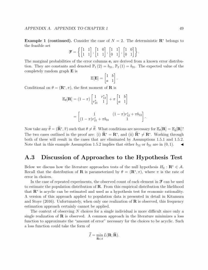
APPENDIX A. APPENDIX TO CHAPTER 1 49
Example 1 (continued). Consider the case of N = 2. The deterministic R∗ belongs tothe feasible set
F =
{[1 11 1
],
[1 01 1
],
[1 10 1
],
[1 00 1
]}.
The marginal probabilities of the error columns ei are derived from a known error distribu-tion. They are constants and denoted P1 (2) = b21, P2 (1) = b21. The expected value of thecompletely random graph E is
E[E] =
[1 ba 1
].
Conditional on θ = (R∗, π), the first moment of R is
Eθ[R] = (1− π)
[1 r∗12r∗21 1
]+ π
[1 ba 1
]
=
[1 (1− π)r∗12 + πb12
(1− π)r∗21 + πb21 1
].
Now take any θ = (R∗, π) such that θ 6= θ. What conditions are necessary for Eθ[R] = Eθ[R]?
The two cases outlined in the proof are: (i) R∗ = R∗, and (ii) R∗ 6= R∗. Working throughboth of these will result in the cases that are eliminated by Assumptions 1.5.1 and 1.5.2.Note that in this example Assumption 1.5.2 implies that either b12 or b21 are in (0, 1). J
A.3 Discussion of Approaches to the Hypothesis Test
Below we discuss how the literature approaches tests of the null hypothesis H0 : R∗ ∈ A.Recall that the distribution of R is parameterized by θ = (R∗, π), where π is the rate oferror in choices.
In the case of repeated experiments, the observed count of each element in F can be usedto estimate the population distribution of R. From this empirical distribution the likelihoodthat R∗ is acyclic can be estimated and used as a hypothesis test for economic rationality.A version of this approach applied to population data is presented in detail in Kitamuraand Stoye (2016). Unfortunately, when only one realization of R is observed, this frequencyestimation approach certainly cannot be applied.
The context of observing N choices for a single individual is more difficult since only asingle realization of R is observed. A common approach in the literature minimizes a lossfunction to approximate the “amount of error” necessary for the choices to be acyclic. Sucha loss function could take the form of
I = minR∈A
L(R; R).
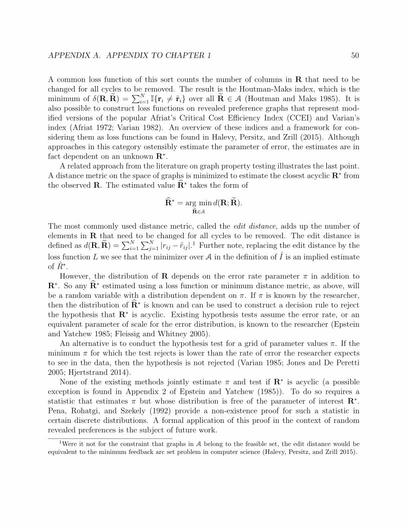
APPENDIX A. APPENDIX TO CHAPTER 1 50
A common loss function of this sort counts the number of columns in R that need to bechanged for all cycles to be removed. The result is the Houtman-Maks index, which is theminimum of δ(R, R) =
∑Ni=1 I{ri 6= ri} over all R ∈ A (Houtman and Maks 1985). It is
also possible to construct loss functions on revealed preference graphs that represent mod-ified versions of the popular Afriat’s Critical Cost Efficiency Index (CCEI) and Varian’sindex (Afriat 1972; Varian 1982). An overview of these indices and a framework for con-sidering them as loss functions can be found in Halevy, Persitz, and Zrill (2015). Althoughapproaches in this category ostensibly estimate the parameter of error, the estimates are infact dependent on an unknown R∗.
A related approach from the literature on graph property testing illustrates the last point.A distance metric on the space of graphs is minimized to estimate the closest acyclic R∗ fromthe observed R. The estimated value R∗ takes the form of
R∗ = arg minR∈A
d(R; R).
The most commonly used distance metric, called the edit distance, adds up the number ofelements in R that need to be changed for all cycles to be removed. The edit distance isdefined as d(R, R) =
∑Ni=1
∑Nj=1 |rij − rij|.1 Further note, replacing the edit distance by the
loss function L we see that the minimizer over A in the definition of I is an implied estimateof R∗.
However, the distribution of R depends on the error rate parameter π in addition toR∗. So any R∗ estimated using a loss function or minimum distance metric, as above, willbe a random variable with a distribution dependent on π. If π is known by the researcher,then the distribution of R∗ is known and can be used to construct a decision rule to rejectthe hypothesis that R∗ is acyclic. Existing hypothesis tests assume the error rate, or anequivalent parameter of scale for the error distribution, is known to the researcher (Epsteinand Yatchew 1985; Fleissig and Whitney 2005).
An alternative is to conduct the hypothesis test for a grid of parameter values π. If theminimum π for which the test rejects is lower than the rate of error the researcher expectsto see in the data, then the hypothesis is not rejected (Varian 1985; Jones and De Peretti2005; Hjertstrand 2014).
None of the existing methods jointly estimate π and test if R∗ is acyclic (a possibleexception is found in Appendix 2 of Epstein and Yatchew (1985)). To do so requires astatistic that estimates π but whose distribution is free of the parameter of interest R∗.Pena, Rohatgi, and Szekely (1992) provide a non-existence proof for such a statistic incertain discrete distributions. A formal application of this proof in the context of randomrevealed preferences is the subject of future work.
1Were it not for the constraint that graphs in A belong to the feasible set, the edit distance would beequivalent to the minimum feedback arc set problem in computer science (Halevy, Persitz, and Zrill 2015).

APPENDIX A. APPENDIX TO CHAPTER 1 51
A.4 Discussion of β and γ
For a fixed π, Eθ[C2(R)] increases with γ and β.2 It is therefore worth exploring the propertiesof β and γ before proceeding. For ease of exposition, suppose the feasible set consists of alldirected graphs on N vertices. The following statements may not hold for a different F
although they provide useful insights on the behavior of the moment condition. Formalexploration of these observations will be an interesting subject of future research.
It is not always the case that every γ ∈ Γ(A) is less than every γ′ ∈ Γ(Ac). Although Ido not prove this formally, the following provides a general intuition. For an acyclic graphR∗ with m < N − 1 edges, a 2-cycle is formed by adding a single edge. There are m cyclicgraphs R∗ constructed by closing a cycle with each of the edges in R∗. Each of these cyclicgraphs has γ(R∗) ≥ γ(R∗). Consider now a second acyclic graph R∗∗ with at least m + 2edges. Since γ captures the interaction between the deterministic graph and the errors, it isreasonable to suppose that one of the cyclic graphs R∗ has a γ(R∗) < γ(R∗∗).
So the sets Γ(A) and the set Γ(Ac) will generally overlap. The existence of an overlapdepends on the feasible set F and the distribution of E on F. An implication is that theexpected number of 2-cycles under the null is not necessarily less than the expected numberof 2-cycles under the alternative hypothesis, even with the contribution of α to the latter.It is possible to construct a cyclic graph whose γ is lower than that of a cyclic graph withmany edges corresponding to high-probability error edges. 3
Consider Γ(F), in which Γ(A) and Γ(Ac) are subsets. Where does β fall? The expectednumber of 2-cycles in E is β, while γ is the expected number of 2-cycles in the union of Eand R∗. Recalling the formulas defined in the previous section, β is summed over i < j whileγ is summed over i 6= j, which may lead us to believe that β < γ(R∗). However, dependingon the distribution of E and F, there may be graphs R∗, either cyclic or acyclic, for whichβ > γ(R∗).
Example 2 (continued). Suppose we observe the three choices in the figure below. Theobserved choices from two budget sets B1 and B2 result in an observed R that has a cycle.
𝐱2
𝐱1
𝐱3
ℬ2
ℬ1ℬ3
𝐑 =1 1 11 1 10 0 1
2With a slight abuse of notation, let γ be an element of the set Γ.3There is a relationship between γ(R∗) and the number of edges in R∗, and adding edges to R∗ results
in a higher γ. However, because of the heterogeneity of the error distribution, there are graphs with feweredges than R∗ that may have γ > γ(R∗).

APPENDIX A. APPENDIX TO CHAPTER 1 52
The seven acyclic feasible graphs are
A =
1 0 0
1 1 11 0 1
,1 0 0
1 1 10 0 1
,1 0 1
1 1 10 0 1
,1 0 0
0 1 10 0 1
,1 0 1
0 1 10 0 1
,1 1 0
0 1 10 0 1
,1 1 1
0 1 10 0 1
.
Suppose further that the error distribution results in the expected value of the random errorgraph E below.
E[E] =
1 0.5 0.750.4 1 10.2 0 1
From E[E] it is possible to find the expected number of 2-cycles in E,
β = 0.35.
Each graph R∗ ∈ A results in a different value of γ(R∗). In the same order as A,
Γ(A) = {1.25, 0.5, 0.7, 0, 0.2, 0.4, 0.6}
Considering the alternative hypothesis, the five cyclic feasible graphs are
Ac =
1 0 1
1 1 11 0 1
,1 1 0
1 1 11 0 1
,1 1 1
1 1 11 0 1
,1 1 0
1 1 10 0 1
,1 1 1
1 1 10 0 1
For these graphs, the set of γ’s is
Γ(Ac) = {1.45, 1.65, 1.85, 0.9, 1.1}
As we can see, the bounds of Γ(Ac) and Γ(A) overlap. However, the minimum of Γ(A), 0.2,is less than the minimum of Γ(Ac), 0.9. Additionally, the maximum of Γ(Ac), 1.85, is greaterthan the maximum of Γ(A), 1.25. There are γ ∈ Γ(A) that are greater than β, and thosethat are less than β. J
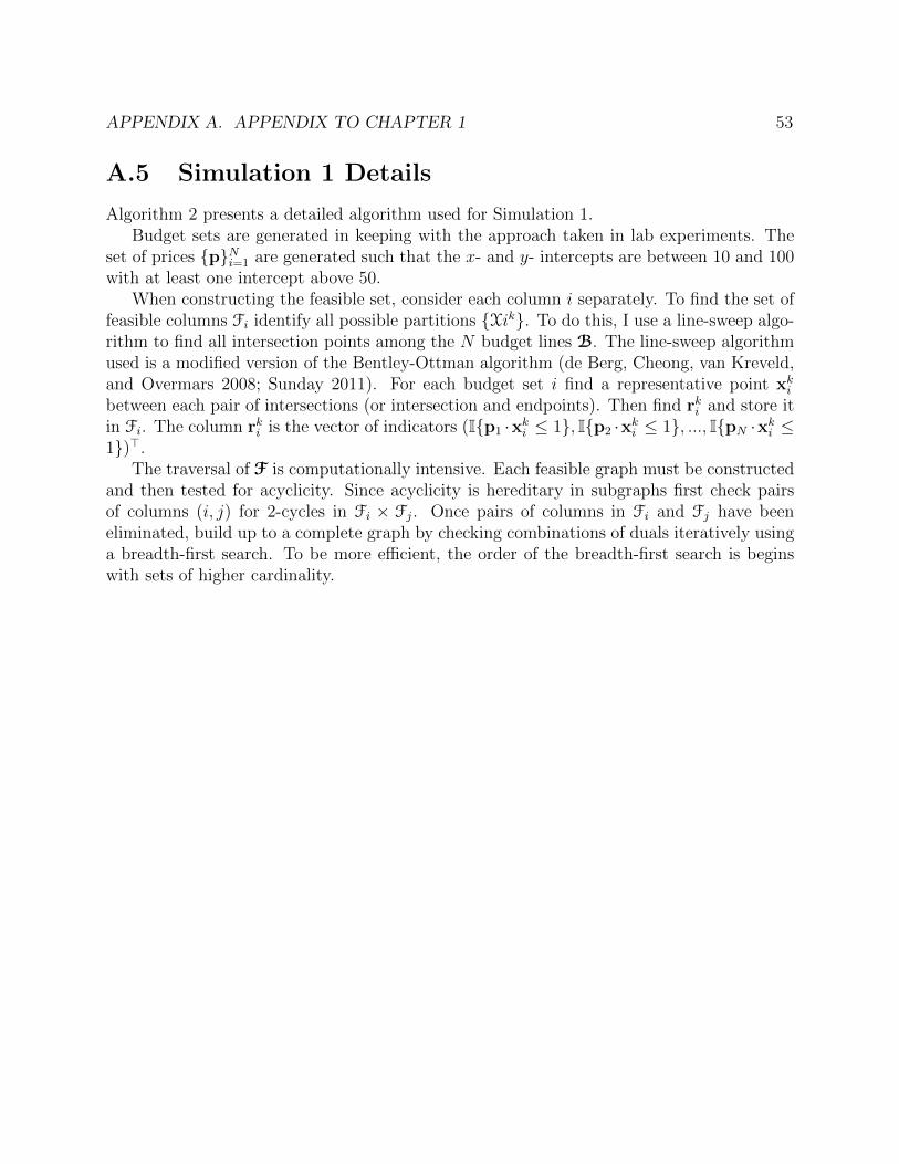
APPENDIX A. APPENDIX TO CHAPTER 1 53
A.5 Simulation 1 Details
Algorithm 2 presents a detailed algorithm used for Simulation 1.Budget sets are generated in keeping with the approach taken in lab experiments. The
set of prices {p}Ni=1 are generated such that the x- and y- intercepts are between 10 and 100with at least one intercept above 50.
When constructing the feasible set, consider each column i separately. To find the set offeasible columns Fi identify all possible partitions {Xik}. To do this, I use a line-sweep algo-rithm to find all intersection points among the N budget lines B. The line-sweep algorithmused is a modified version of the Bentley-Ottman algorithm (de Berg, Cheong, van Kreveld,and Overmars 2008; Sunday 2011). For each budget set i find a representative point xkibetween each pair of intersections (or intersection and endpoints). Then find rki and store itin Fi. The column rki is the vector of indicators (I{p1 ·xki ≤ 1}, I{p2 ·xki ≤ 1}, ..., I{pN ·xki ≤1})>.
The traversal of F is computationally intensive. Each feasible graph must be constructedand then tested for acyclicity. Since acyclicity is hereditary in subgraphs first check pairsof columns (i, j) for 2-cycles in Fi × Fj. Once pairs of columns in Fi and Fj have beeneliminated, build up to a complete graph by checking combinations of duals iteratively usinga breadth-first search. To be more efficient, the order of the breadth-first search is beginswith sets of higher cardinality.

APPENDIX A. APPENDIX TO CHAPTER 1 54
Algorithm 2: Detailed pseudocode for Simulation 1
N : sample sizeL : dimension of choice space
1 Randomly Generate B
Return: N budget sets Bi defined by pi ∈ RL++
2 Construct F
forall (Bi ∈ B) doFind all Ki partitions {Xk
i } pf ∂↑Bi
foreach Xki do
Find the “revealed to” column ri
Return: N sets of feasible columns Fi
3 Calculate E[E]foreach Fi do
Calculate E[ei] according to fei on support Fi
Return: N ×N matrix of marginal probabilities for E
4 Construct Γ(A)
forall (R ∈ F) do
if R is acyclic then
Solve for γ(R) as a function of R and E[E]
Return: vector of numbers of length |A|5 Calculate true choices
Input: Utility function u(·)forall (Bi ∈ B) do
Solve for x ∈ ∂↑Bi that maximizes u(x)
Return: set of N true choices {x∗i }6 Simulate M repeated samples
Input: error rate πfor (m in {1, ...,M}) do
for (i in {1, ..., N}) doRandomly generate zi ∼ Bernoulli(π)Randomly generate ui ∼ Fui
Construct observed ri from xi = (1− zi)x∗i + ziui and B
Calculate the number of two cycles C2(Rm) for the m repetition
Return: C2, the average over all {C2(Rm)} M repetitions
7 Estimate {π(γ)}|A for all γ ∈ Γ(A)

55
Appendix B
Appendix to Chapter 2
B.1 Monte Carlo Simulations
Table B.1: Comparing the performance of different two-sided tests at α = 5%
Kolmogorov- Mann- Anderson- at leastSmirnov Whitney Darling one test all tests
reject under 0.049 0.049 0.028 0.077 0.049 – –null hypothesis
fail to reject 0.520 0.567 0.528 – – 0.474 0.513under alternative
p-value threshold 0.05 0.05 0.05 0.05 0.035 0.05 0.035
The results above were measured from 1000 Monte Carlo simulations. The first row in-dicates the fraction of simulations in which the null hypothesis was rejected, even thoughthe distributions were the same. The second row indicates the percentage of simulationsin which the null was not rejected, although the distributions were different. The first fourcolumns show rates for individual tests, and the last two columns show rates for at least oneof the four tests. All tests were two-sided and used a p-value threshold of 0.05, except forthe last column in which the threshold was 0.035.
Simulation details: In each simulation two samples (of sizes 120 and 150) were drawn fromdifferent distributions. The distributions were generated randomly to emulate the patternseen in the data: a mixture of a Beta distribution contaminated with a mass point on 1.Under the null hypothesis both distributions were the same. The shape parameters rangedfrom 5 to 15, and from 0.4 to 0.6; the contamination occurred with a 0.2 probability. Under
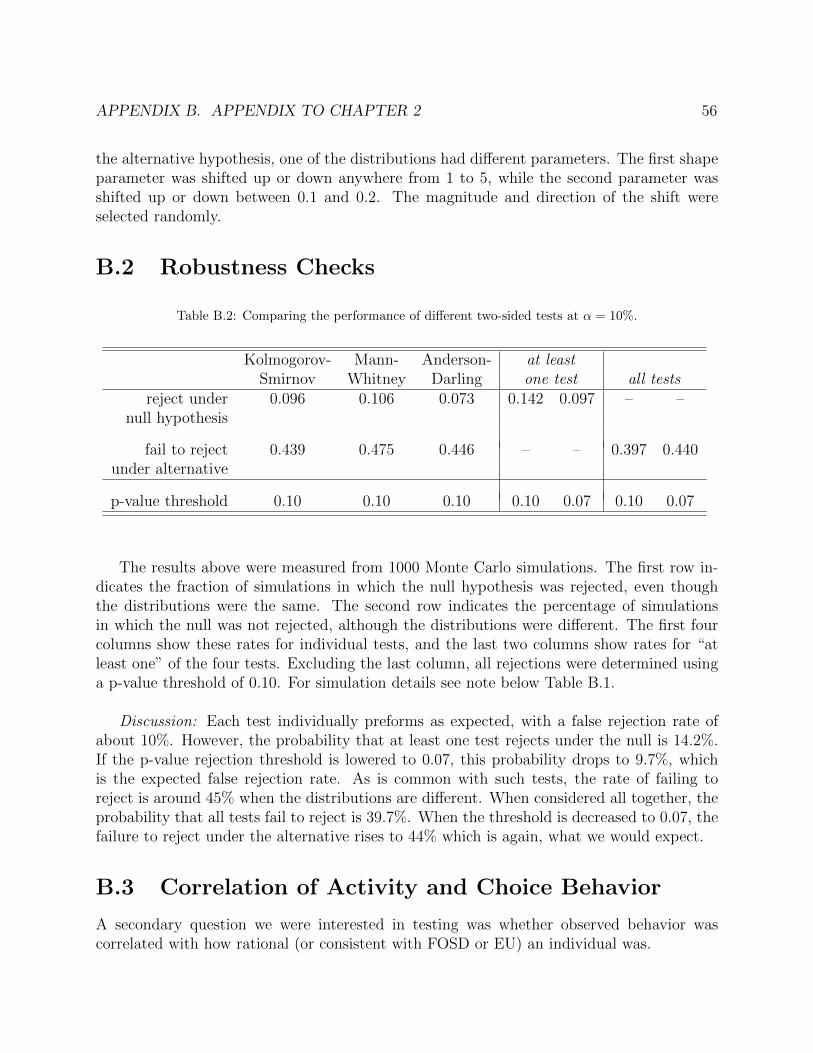
APPENDIX B. APPENDIX TO CHAPTER 2 56
the alternative hypothesis, one of the distributions had different parameters. The first shapeparameter was shifted up or down anywhere from 1 to 5, while the second parameter wasshifted up or down between 0.1 and 0.2. The magnitude and direction of the shift wereselected randomly.
B.2 Robustness Checks
Table B.2: Comparing the performance of different two-sided tests at α = 10%.
Kolmogorov- Mann- Anderson- at leastSmirnov Whitney Darling one test all tests
reject under 0.096 0.106 0.073 0.142 0.097 – –null hypothesis
fail to reject 0.439 0.475 0.446 – – 0.397 0.440under alternative
p-value threshold 0.10 0.10 0.10 0.10 0.07 0.10 0.07
The results above were measured from 1000 Monte Carlo simulations. The first row in-dicates the fraction of simulations in which the null hypothesis was rejected, even thoughthe distributions were the same. The second row indicates the percentage of simulationsin which the null was not rejected, although the distributions were different. The first fourcolumns show these rates for individual tests, and the last two columns show rates for “atleast one” of the four tests. Excluding the last column, all rejections were determined usinga p-value threshold of 0.10. For simulation details see note below Table B.1.
Discussion: Each test individually preforms as expected, with a false rejection rate ofabout 10%. However, the probability that at least one test rejects under the null is 14.2%.If the p-value rejection threshold is lowered to 0.07, this probability drops to 9.7%, whichis the expected false rejection rate. As is common with such tests, the rate of failing toreject is around 45% when the distributions are different. When considered all together, theprobability that all tests fail to reject is 39.7%. When the threshold is decreased to 0.07, thefailure to reject under the alternative rises to 44% which is again, what we would expect.
B.3 Correlation of Activity and Choice Behavior
A secondary question we were interested in testing was whether observed behavior wascorrelated with how rational (or consistent with FOSD or EU) an individual was.

APPENDIX B. APPENDIX TO CHAPTER 2 57
Native apps present a unique opportunity for the researcher to observe subject behavior“in the wild” passively using built-in sensors. To this end we collected activity data passivelyfrom the subject’s mobile phones over the same 5 day period. The data consists of phonelogs, location logs, and battery usage. The phone log is a time-stamped list of all callsand texts sent and received. For each call or text the log records the correspondent phonenumber, duration (for calls), and status (incoming or outgoing)1. The location logs are atimestamped list of the latitude and longitude, sampled approximately every 30 seconds.Additionally, battery level and charging status were sampled when a choice was submittedby the subject.
From the resultant rich dataset, we extract numerous features that summarize an indi-vidual’s activity over the 5 day experimental period. We base social activity on SMS dataand exclude call data from our analysis due to relative usage patterns, consistent with theage group of the participants. The features measure responsiveness in SMS behavior (SMSmean latency), as well as breadth of contacts (SMS entropy). The location logs were firstprocessed to identify movement and stationary periods. Physical activity was then mea-sured as the number of unique stationary locations (number of activities, ratio of activitiesnight:day) as well as total time spent in motion (time moving, percent of time in transit).Detailed descriptions and summary statistics can be found in the online appendix [createsummary stats appendix].
Lastly, a demographic questionnaire was administered to the second half of the lab-in-fieldparticipants. The subjects’ intended major, age, and gender were collected.
Unfortunately, we do not find any significant results correlating rationality with activitydata.
1All data was encrypted on the phone prior to being sent to our server, which was also encrypted. Inaddition, to preserve privacy of third party individuals who had not consented to participate in our study,all phone numbers collected in the call log were made anonymous up to the area code.)