Measuring an IP Network in situ

Hal Burch

May 6, 2005

CMU-CS-05-132

School of Computer ScienceCarnegie Mellon University

Pittsburgh, PA 15213

Submitted in partial fulfillment of the requirementsfor the degree of Doctor of Philosophy

Thesis Committee

Bruce MaggsGary L. Miller

Srinivasan SeshanSteven Bellovin

c©2005, Hal Burch

Some of this material is based upon work funded under a National Science Foundation Graduate ResearchFellowship. Also partially funded by NSF Nets Grant CNF-0435382, ARPA Contract N00014-95-1-1246, and NSFNYI Award CCR-94-57766, with matching funds provided by NEC Research Institute and Sun Microsystems. Anyopinions, findings, conclusions, or recommendations expressed in this publication are those of the author and do notnecessarily reflect the views of any funding agency or organization.

Keywords: networking measurement,network topology,graph drawing,tomography,traceback,IPaliasing,reverse traceroute,anonymous DNS

Abstract

The Internet, and IP networking in general, have become vital to the scientific community andthe global economy. This growth has increased the importance of measuring and monitoring theInternet to ensure that it runs smoothly and to aid the design of future protocols and networks. Tosimplify network growth, IP networking is designed to be decentralized. This means that each routerand each network needs and has only limited information about the Internet. One disadvantageof this design is that measurement systems are required in order to determine the behavior of theInternet as a whole.

This thesis explores ways to measure five different aspects of the Internet. The first aspectconsidered is the Internet’s topology, the inter-connectivity of the Internet. This is one of thebasic questions about the Internet: what hosts are on the Internet and how are they connected?The second aspect is routing: what are the routing decisions made by routers for a particulardestination? The third aspect is locating the source of a denial-of-service (DoS) attack. DoSattacks are problematic to locate because their source is not listed in the packets. Thus, specialtechniques are required. The fourth aspect is link delays. This includes both a general system todetermine link delays from end-to-end measurements and a specific system to perform end-to-endmeasurements from a single measurement host. The fifth aspect is the behavior of filtering onthe network. Starting about fifteen years ago, to increase security, corporations started placingfiltering devices, i.e., “firewalls”, between their corporate network and the rest of the Internet. Foreach aspect, a measurement system is described and analyzed, and results from the Internet arepresented.

2

Acknowledgements

My friends, family, and colleagues have assisted in many ways. I am unlikely to be able to properlyenumerate the contribution of each. I will thus limit myself to these few:

My advisors, Bruce Maggs and Gary L. Miller, have helpfully guided and directed me through-out my tenure at Carnegie Mellon.

My colloborators, Chris Chase, Dawn Song, Bill Cheswick, Steven Branigan, and Frank Wojcik,contributed greatly to much work here-in.

My wife, Kimberly Jordan Burch, supported me, both emotionally and linguistically, fixing myEnglish errors.

Phil Gibbons, Linda Moya, and Tim and Jen Coles opened their homes to me to allow me tocontinue to visit Carnegie Mellon on a regular basis while living with my wife in New Jersey. AT&Tprovided me with a workspace while in New Jersey.

3

4

Contents

1 Introduction 7

2 Network Mapping 11

2.1 Motivation . . . . . . . . . . . . . . . . . . . . . . . . . . . . . . . . . . . . . . . . . 12

2.2 Network Mapping . . . . . . . . . . . . . . . . . . . . . . . . . . . . . . . . . . . . . . 13

2.3 Map Layout . . . . . . . . . . . . . . . . . . . . . . . . . . . . . . . . . . . . . . . . . 15

2.4 Watching Networks Under Duress . . . . . . . . . . . . . . . . . . . . . . . . . . . . . 19

2.5 Related Work . . . . . . . . . . . . . . . . . . . . . . . . . . . . . . . . . . . . . . . . 22

2.6 Corporate Networks . . . . . . . . . . . . . . . . . . . . . . . . . . . . . . . . . . . . 23

2.7 Conclusion . . . . . . . . . . . . . . . . . . . . . . . . . . . . . . . . . . . . . . . . . 23

3 IP Resolution 25

3.1 Methodology . . . . . . . . . . . . . . . . . . . . . . . . . . . . . . . . . . . . . . . . 26

3.2 Splitting Methods . . . . . . . . . . . . . . . . . . . . . . . . . . . . . . . . . . . . . 29

3.3 UDP Technique . . . . . . . . . . . . . . . . . . . . . . . . . . . . . . . . . . . . . . . 32

3.4 IPid Technique . . . . . . . . . . . . . . . . . . . . . . . . . . . . . . . . . . . . . . . 33

3.5 Rate Limit Technique . . . . . . . . . . . . . . . . . . . . . . . . . . . . . . . . . . . 38

3.6 Experimental Results . . . . . . . . . . . . . . . . . . . . . . . . . . . . . . . . . . . . 41

3.7 Conclusions . . . . . . . . . . . . . . . . . . . . . . . . . . . . . . . . . . . . . . . . . 46

4 Estimating the Reverse Routing Map 47

4.1 Previous Work . . . . . . . . . . . . . . . . . . . . . . . . . . . . . . . . . . . . . . . 48

4.2 TTL Method . . . . . . . . . . . . . . . . . . . . . . . . . . . . . . . . . . . . . . . . 49

4.3 Results . . . . . . . . . . . . . . . . . . . . . . . . . . . . . . . . . . . . . . . . . . . . 51

4.4 Conclusions . . . . . . . . . . . . . . . . . . . . . . . . . . . . . . . . . . . . . . . . . 56

5

5 Tracing Anonymous Packets 59

5.1 Basic Technique . . . . . . . . . . . . . . . . . . . . . . . . . . . . . . . . . . . . . . . 60

5.2 Assumptions . . . . . . . . . . . . . . . . . . . . . . . . . . . . . . . . . . . . . . . . 61

5.3 Network Load: No Gain, No Pain . . . . . . . . . . . . . . . . . . . . . . . . . . . . . 62

5.4 Results . . . . . . . . . . . . . . . . . . . . . . . . . . . . . . . . . . . . . . . . . . . . 67

5.5 Alternative Strategies . . . . . . . . . . . . . . . . . . . . . . . . . . . . . . . . . . . 67

5.6 Ethics . . . . . . . . . . . . . . . . . . . . . . . . . . . . . . . . . . . . . . . . . . . . 69

5.7 Later Work . . . . . . . . . . . . . . . . . . . . . . . . . . . . . . . . . . . . . . . . . 70

5.8 Conclusions . . . . . . . . . . . . . . . . . . . . . . . . . . . . . . . . . . . . . . . . . 71

6 Monitoring Link Delays with One Measurement Host 73

6.1 Related Work . . . . . . . . . . . . . . . . . . . . . . . . . . . . . . . . . . . . . . . . 75

6.2 Measurement System . . . . . . . . . . . . . . . . . . . . . . . . . . . . . . . . . . . . 75

6.3 Tomography Technique . . . . . . . . . . . . . . . . . . . . . . . . . . . . . . . . . . 78

6.4 Results . . . . . . . . . . . . . . . . . . . . . . . . . . . . . . . . . . . . . . . . . . . . 83

6.5 Future Work . . . . . . . . . . . . . . . . . . . . . . . . . . . . . . . . . . . . . . . . 91

6.6 Conclusions . . . . . . . . . . . . . . . . . . . . . . . . . . . . . . . . . . . . . . . . . 92

7 Firewall Configuration and Anonymous DNS 95

7.1 Previous Work . . . . . . . . . . . . . . . . . . . . . . . . . . . . . . . . . . . . . . . 97

7.2 Methodology . . . . . . . . . . . . . . . . . . . . . . . . . . . . . . . . . . . . . . . . 97

7.3 Results . . . . . . . . . . . . . . . . . . . . . . . . . . . . . . . . . . . . . . . . . . . . 104

7.4 Conclusions . . . . . . . . . . . . . . . . . . . . . . . . . . . . . . . . . . . . . . . . . 117

8 Conclusions 119

6

Chapter 1

Introduction

The Internet has grown from a small research network to a global network used by businesses,individuals, and researchers. In December 1969, the Internet (then known as ARPANET) con-sisted of only four nodes: UCLA, UCSB, Stanford Research Institute, and the University of Utah.From these humble beginnings, the Internet has grown to hundreds of millions of hosts on tens ofthousands of networks. This growth in size has been coupled with a growth in the importance ofthe Internet. According to Cisco[20], $830 billion of revenue was generated over the Internet in2000. That exceeds the GDP of all but thirteen countries. With the introduction of broadbandto households, services that traditionally ran on other networks, such as voice and video, are in-creasingly moving to the Internet. For voice, this migration has already begun, with major cablecompanies offering voice over IP (VoIP) service to consumers. This increasing dependence on theInternet for communication and commerce means that the Internet is becoming vital to nationaland world economies.

As the Internet grows in importance, the ability to monitor and measure it effectively alsogrows. The same growth that increases the importance of the Internet however, also makes theInternet more difficult to monitor. When the Internet began as the ARPANET, it had only oneservice provider. Today, the Internet has thousands to tens of thousands of service providers. Tohandle this growth, the Internet is built as a network of networks designed to make it easy for anew network to join with minimal configuration changes. To facilitate this, each router operateswhile maintaining only limited information. This decentralized design means that the Internet hasbeen able to grow without over-burdening the routers with both static and dynamic configurationinformation. This localization of information makes it more difficult to understand the globalbehavior of the Internet, as each router has only limited data. Understanding the behavior of thenetwork requires building measurement systems to collect the necessary information.

Measurement systems do much more than merely satisfy intellectual curiosity about the Inter-net. Measurement systems are necessary for operation, architecture, protocol design, and protocolimplementation. Internet service providers and companies with corporate IP networks must mea-sure their network to ensure that it is operating properly, and will continue to operate properly.They must make certain that all nodes in the network can communicate properly, that sufficientbandwidth exists to meet the needs of the network, and that the network is sufficiently secure.Network architects want to know what is happening on the current network in order to design themost efficient network they can and to ensure the network meets the demands placed on it.

7

Protocol designers often face the daunting task of designing a protocol that will work when runby hundreds of millions of hosts. They must do this while being able to test it on only hundredsto thousands of hosts. For this reason, protocol designers often turn to analysis and simulation inorder to stress their protocols with large-deployment scenarios. It is important to understand theInternet, as neither analysis nor simulation is useful if the assumptions on which they are basedare flawed. Protocol implementors face similar problems, but must additionally deal with fieldfaults that result from implementation error. Good simulation tools can simplify the problem ofdetermining the cause of a field fault and finding a remedy for it. Moreover, having a simulationthat closely reflects reality makes it more likely that implementors can find and repair bugs beforethey are deployed.

Building measurement systems often involves finding ways to extract information from availablebehaviors. To date, designers of Internet protocols have paid only limited attention to includingways to measure the systems they are building. Instead, protocol designers generally focus onthe problem of building a networking system that scales to hundreds of millions of hosts whilemaintaining high reliability, low latency, and a high level of robustness. This focus is proper, asa precisely measurable system is of little use if it does not work. Even when a protocol includesmonitoring features, it is difficult for protocol designers to predict everything that a user may wantto monitor.

Although one might think that monitoring features could simply by added to the protocol, real-ity is not that simple. Changing the protocol requires each vendor to change their implementationof the protocol and then each system administrator to update their hosts to run the new protocol.A protocol, once defined by standards or practice, can have dozens of implementations and bedeployed on thousands or millions of hosts. Convincing all vendors and administrators is difficultat best for widely-deployed protocols. Even if they can be convinced, a change in a protocol cantake years or longer to become widely deployed. The most obvious example of this is IPv6[27],which was first proposed in 1995, but continues to have limited deployment. Any realistic methodof measuring the Internet cannot require a change to the protocols running on more than a few endsystems. This limitation often means that measurement methods often find a new way to extractuseful information from an existing feature of a protocol.

An example of using existing features in an unusual way is traceroute[46]. Traceroute is a vitalmeasurement tool that has long been used by network administrators to identify the path takenby outgoing packets towards a given destination. Traceroute works by sending packets with lowtime-to-live (TTL) values. After the packet has traveled through a number of routers equal to theinitial TTL value, the next router will discard the packet. When discarding such packets, mostrouters will return a ICMP error packet[75], which includes an IP address of the router sending thepacket. By varying the TTL value, traceroute determines the routers along the path.

Traceroute is commonly employed to determine the cause of network difficulties. If packets arenot delivered, the last responsive hop in the path indicates the source of the problem. By examiningthe round-trip-times of the traceroute probes, sources of high latency can often be identified. Inaddition, traceroute readily identifies routing loops, which occur when a set of routers becomeconfused about the path to a particular destination. The resulting path, like the snake Uroboros,swallows its own tail and becomes a loop. Routing loops are one of main reasons the TTL fieldexists. Without the TTL field, the packet would cycle endlessly in the loop, stopping only if atransmission error occurred or the path corrected itself.

This dissertation presents ways to measure the Internet within the constraints of the current

8

infrastructure. It begins with Chapters 2 and Chapter 3, which address measuring the topology.Chapter 2 addresses the problem of collecting and presenting IP-level topology information onthe Internet or any IP-based network. Chapter 3 considers the problem of determining if two IPaddresses represent the same host, which can be used to refine topologies by combining multipleIP addresses belonging to the same host.

Chapters 4 and 5 utilize topology information for other measurements. Chapter 4 presentsan algorithm to estimate the routing towards a particular destination. The algorithm results inrouting estimations for a much larger fraction of the Internet than previously-known techniques.The algorithm is analyzed for its coverage and accuracy and compared against those techniques.Chapter 5 describes a (rather evil) method to determine the source of a stream of spoofed packets,common in denial-of-service attacks. It also includes several other schemes to determine the sourceof such streams or to disallow the production of such streams in the first place. It includes a briefoverview of research subsequent to its publication.

The remaining chapters focus on other measurement problems. Chapter 6 gives a method fordetermining individual link delays from end-to-end measurements. This is commonly of interest toISPs and other network operators, as it tells them how well their network is performing. Chapter7 examines common firewall behavior, as observed from the Internet. This provides insight intothe concerns and attitudes of firewall administrators. Such information is also useful to protocoldesigners, which much be sensitive to firewall behaviors. Chapter 8 ends the dissertation withconclusions.

9

10

Chapter 2

Network Mapping1

One of the basic measures of a network is its connectivity. Having no knowledge of the hostsand links in the network makes information about the behavior of hosts or links nearly useless.It is unclear what the proper questions are to ask about the hosts or links if their relationshipsare not known. Any available information is difficult to interpret or use without knowing thestructure. This chapter describes the Internet Mapping Project, an attempt to measure and recordthe topology of the Internet and how it changes over years.

The basic technology used by the Internet Mapping Project (IMP) is traceroute[46]. Traceroutegives the set of hops from one host to another. Modulo a few caveats discussed later, adjacent hopsin the resulting path are connected by a link. The topology can, at least in theory, be determinedby taking a large set of traceroute paths and taking the union. By taking a list of all announcednetwork on a network, such as the Internet, and discovering the path to each of these networks, agood picture of the “center” of the network can be built. This provides a kind of picture of whatthe network looks like as a whole. Of course, this is an egocentric view, as it captures the pathstaken by packets outgoing from the measurement host. Thus, the picture is a reachability graph,not a complete map.

The Internet Mapping Project measures the Internet using this process. Every morning, themapping program of the IMP measures the topology of the Internet. The Internet data is archivedon CD-ROMs. Scans have been run daily since they began in August, 1998. This scanning detectslong-term routing and connectivity changes on the Internet. Daily scans are likely to miss a shortoutage of a major backbone that lasts for only a few hours, unless it happens during a scan. Eventsthat happen on larger time scales, such as a natural disaster, war, or a major act of terrorism, arelikely to show up.

Due to the magnitude of the resulting databases, a method of visualizing it is required, allowingthe eye to improve the understanding of the collected data. The visualization makes it possible topick out interesting features for further investigation and find errors in Internet router configura-tions, such as routers that return invalid IP addresses. It would be desirable to have a large papermap with the properties of traditional flat maps: helpful when navigating towards destinations,

1This chapter represents work with William Cheswick and Steven Branigan, first published as “Mapping andVisualizing the Internet” in 2000 USENIX Annual Technical Conference[17]. A later article was also published inIEEE Computer[7]

11

display connectivity, readily reveal major features and interesting relationships, and are hard tofold up.

IMP’s layout algorithm uses a spring-force algorithm to position the nodes on the map. A fewsimple rules govern the adjustment of a point’s position based on proximity of graph neighbors,number of incident edges, and the number and position of close nodes that are not neighbors. WhenIMP began, the Internet graph had 88,107 nodes and 99,664 edges. The points were shuffled for20 hours on a 400MHz Pentium to obtain the maps shown in this chapter. The Internet graph hasgrown to 153,133 nodes and 183,144 edges today. The nodes are still shuffled for 20 hours to layoutthe graph, but now those 20 hours take place on a 1 GHz Pentium III box.

In the course of developing and testing the mapping software, it become apparent that map-ping is a more generally useful pursuit. Large corporate networks are difficult to manage and offermany security problems. Often, local changes in the network may not be properly communicatedto the central administrators. For example, if a division of a company needs to communicate withanother company, that division may purchase a connection to the other company, and set-up theirlocal network to allow communication. The network, detecting the change, may reconfigure theentire network to be able to communicate with the newly-connected company. Because networksare designed to be robust to network changes, this can occur without action by the central ad-ministrators. The net effect of such a change is that anyone in the newly connected company cancommunicate with any host within the network. This free access is a security problem. Firstly, anyvirus, worm, or hacker that infiltrates the new company has access to the network. Secondly, oftentwo cooperating companies compete in many areas, making free access extremely undesirable. Amap of a company’s network topology can yield substantial information and can help spot likelyleaks in a company’s perimeter security.

2.1 Motivation

The initial motivation for collecting path data came out of a Highlands Forum, a meeting thatdiscussed possible responses to future infrastructure attacks using a scenario from the Rand Corpo-ration. It was clear that a knowledge of the Internet’s topology might be useful to law enforcementif the nation’s infrastructure was under attack. It might be useful to know how connectivity changesbefore and during an attack on the Internet infrastructure. The Internet topology could also beuseful for tracking anonymous packets back to their source, as will be discussed in Chapter 5. Inaddition, an openly-available map could be useful to monitor the connectivity of the Internet, andwould be helpful to a variety of investigators.

Good ISPs already watch this kind of information in near real-time to monitor the health oftheir own networks, but they rarely know anything (or care much) about the status of networks thatare not directly connected to theirs. No one is responsible for watching the whole Internet. Givenits size, the entire Internet would be difficult to watch. There is a major web of interconnectingISPs that in some sense defines the “middle” of the net—the most important part. The InternetMapping Project grew out of attempts to map this middle. It uses traceroute-style packets, whichmeans that it only maps outgoing paths, and only from the measurement host—these limitationsare discussed below. Even this limited connectivity information can yield insights about who isconnected to whom.

12

0

20000

40000

60000

80000

100000

120000

140000

160000

180000

200000

01/01/1998 01/01/1999 01/01/2000 01/01/2001 01/01/2002 01/01/2003 01/01/2004 01/01/2005

Cou

nt

Date

IMP Graph Size

Edge countNode count

Figure 2.1: Size of the Internet graph, as measured by IMP, in terms of node and edge counts overthe last six years.

The database itself can be useful for routing studies and graph theorists looking for real-worlddata to work with. Since the data is being collected daily over a long period of time, it may bepossible to extract interesting trends. Data is systematically collected daily, building a consistentdatabase that can be used to reconstruct routing on the Internet approximately for any day wheremapping was done, at least the paths from the measurement host.

The mapping software has lent itself to another pressing problem: controlling an intranet.Software that can handle 150,000 nodes on the Internet can easily handle intranets of similar size.An intranet map can be colored to show insecure areas, business units, connections to remoteoffices, etc.

IMP’s visualizations of the Internet itself have attracted wide media interest[10, 105]. Mediagenerally visually represents the Internet by showing people staring at a web browser. The InternetMapping Project’s maps give some idea of the size and complexity of the Internet. Figure 2.1 showshow the number of nodes and edges has grown over the project’s lifetime, giving a rough notion ofthe growth of the Internet.

2.2 Network Mapping

The data from the Internet Mapping Project (IMP) consists of paths from a measurement hosttowards a single host on a destination network. The list of networks on the Internet is the com-bination of four lists. The first list comes from the routing arbiter database[62]. This is a centralregistry of all assigned Internet addresses, including those used only privately. Each provides atarget network address as a CIDR block, such as 135.104.0.0/16. Two other sources of networksare BGP route entries and domain name service delegations. BGP route entries are CIDR blocksalready. Domain name service delegations come from delegation of reverse lookups (in-addr.arpa).A delegation of, say, 2.128.in-addr.arpa corresponds to the CIDR Block 128.2.0.0/16. Although

13

not originally included, both sources have been added since. The fourth list is every class B (/16)CIDR block. This last list provides insurance against the first three sources missing a large network.

The network scanner must traceroute to a particular host, rather than tracing to a CIDR block.As it is not particularly important that the host actually be present, the network scanner randomlypicks an IP number in each CIDR block. This random selection is biased, based on a quick surveyof commonly-used IP addresses (e.g., the most common last octet is 1 and lower numbers are morecommon). If an IP address is found to which the scanner can find a complete traceroute, that IPaddress is recorded and reused. Essentially, the mapping performs a slow host scan over time untila responsive host is found. Even with this slow host scan, most of the network traces end eitherwith silence (due to an nonexistent address or a firewall) or an ICMP error-reported failure. Thelarge number of incomplete paths is largely a result of aggressively including CIDR blocks. Becausetesting an nonexistent CIDR block is both quick and non-intrusive, the gathering process discardsno potential CIDR blocks listed anywhere.

This technique only records an outgoing packet path. The incoming path is often different:many Internet routes are asymmetric, as ISP interconnect agreements often divert traffic throughdifferent connections. Techniques to discover return packet paths are discussed in Chapter 4.

The path may vary between traces, or even individual probes, depending on outages, redundantlinks, reconfigurations, etc. This means the mapping program may occasionally ‘discover’ pathsthat don’t exist. Imagine a packet to Germany that is either routed through the United Kingdom orFrance at random, for example. As alternate packets travel through alternate paths, the mappingprogram will infer connections between the alternate paths that do not exist. Load-balancing overlarge stretches of paths is believed to be rare, making the effect of them limited. In terms ofoutages and routing changes, the number of routes changing during a scan should, in most cases,be relatively small.

The technique employed only discovers the IP path. A single IP-layer link may not represent aphysical link. For example, if an ISP is running their backbone over ATM, then each link representsa virtual circuit that may travel through many ATM nodes. Depending on how the ATM networkis configured, such an ISP’s backbone may appear to be completely connected, even though it isn’tphysically true. From an IP standpoint, however, detecting the physical connectivity is extremelydifficult.

The target, date, path data, and path completion codes are recorded in a simple text format.The database is manipulated with traditional Unix text tools and some simple additional programs.Each day’s database is compressed and stored permanently. Copies are available upon request. Thelatest Internet database was available online, but was taken down over concerns about the data.The database is routinely supplied to researchers, although they receive a database that is a fewmonths old. The database is about 25 MB.

2.2.1 Mapping, Not Hacking

One goal is that the traceroutes are not confused with hacking probes. This means that the mappingmust proceed gingerly. The mapping program probes with ICMP Echo Request packets[75] (ping).Most intrusion detection systems recognize these as ping packets, though the TTL values useddiffer from traditional pings. At worse, the probes tend to confuse system administrators, as thereare few real services that use ping.

14

Originally, the path was discovered one hop at a time. For each hop, a probe was sent out. Ifno reply was received in 5 seconds, a second probe was sent. If no reply was received to the secondprobe in 15 more seconds, a third probe was sent. If no reply was received within 45 seconds afterthe third probe was sent, the path discovery was halted. Stopping a path trace after failing onlyone hop stopped the scanning from discovering the second half of many paths[21], but made thescanning less threatening to network citizens.

Today’s scanner discovers each path in two passes. The first pass tests each hop sequentially,sending only one packet per hop. The first pass ends either when the target is reached or two hopsin a row fail to respond within three seconds. The second pass attempts to fill-in the holes fromthe first pass left by non-responding hops. Each hole is probed twice more, once with a five secondtimeout, and once with a 20 second timeout. This scanning methodology is designed to only sendone more packet across a blocking firewall than the previous technique, while completing morepaths. Allowing one hole completes approximately 4% more of the paths, but will still not scanacross an ISP that configures all of their routers to return no responses to traceroute-like probes.

Another aspect of attempting to make it clear that the mapping traffic is not hacking traf-fic is to enable curious system and network administrators to easily determine what the trafficis. The first clue to them is the name of the measurement host, netmapper, and the domainresearch.lumeta.com. This name itself tells most of the story, and it is believed that this makesmost administrators who do notice the packets nod and move on to other work. A web page de-scribing the project is maintained[57]. A DNS TXT record has been added to netmapper’s entrythat points to IMP’s web page. In addition, all web queries to netmapper are redirected using theworld’s shortest (and safest) web server (the web server just cat’s a file).

A few network administrators have complained. They either did not like the probe, or IMP’spackets cluttered their logs (The Australian Parliament was the first on the list!). These networksare recorded in an opt-out list and cease probing them. Certainly others may have simply blockedIMP’s packets, or filtered IMP’s probes out of their logs. It might be interesting to compare hoststhat were reached early in the scans and later fell out of sight.

A number of emergency response groups made contact asking about the network scanner’sactivity. The goal was for them to understand the mapping activity, thus satisfying their justifiablecuriosity. It would be much harder time justifying the probes if it included overt host or port scans,which often precede a hacking attack. Only a tiny percentage of the Internet system administratorsappear to have noticed the mapping efforts.

The measurement host itself is highly resistant to network invasion: some other network scanshave promoted powerful hacking responses. Of course, like any other publicly-accessible host, itcould fall to denial-of-service attacks.

2.3 Map Layout

A force-directed method similar to previous work[24, 35] is used to lay out the graph. The basicidea is to model the graph as a physical system and then to find the set of node positions that min-imizes the total energy. The standard model employed is spring attraction and electrical repulsion.Attraction is done by connecting any two connected nodes by a spring. The repulsive force derivesby giving each node a positive electrical charge, causing them to repel each other.

15

Finding a minimum of such physical models has been well studied. In particular, the mostcommon techniques are gradient descent[86], conjugate gradient[90], and simulated annealing[86].None of these algorithms are guaranteed to find a global minimum in a reasonable time, but theyare able to find approximately minimum configurations. Because it is easier to code, gradientdescent was selected.

At the time of the development of IMP’s graph layout algorithm, graph drawing work consideredgraphs with a tenth the size of the Internet dataset as huge[39, 100]. Extending the runtime resultsof previous work to IMP’s graph and adjusting for a faster host yields times on the order of monthsto millennia. Thus, the standard algorithms at the time were too slow for IMP’s graph. Two tricksare used to more quickly compute a layout, at the cost of possibly being less optimal.

The first trick is replace the electrical repulsive field with spring repulsion. Imagine that anytwo nodes which do not share an edge are connected, via infinite strings, to a spring. Thus, if thenodes are further apart than the rest length of the spring, there is no force applied. If the nodesare are closer than the spring’s rest length, the spring is compressed, and the nodes are pushedapart. This bounds the repulsive force, which means that instead of having to calculate a quadraticnumber of repulsive forces, the number of repulsive forces goes down to approximately linear, sincepairs of points that are further apart than the rest length can be ignored. Thus, the exact repulsiveforce on each node can be calculated in approximately linear time.

The real optimization, however, is laying out the graph one layer at a time. First the links toIMP’s three ISPs are laid out and the system is iterated until they stop moving “much.” Then, allthe routers one hop further away are added, and the system is iterated (which may move the nodesfrom previous levels as well). Then the next hop, continuing until all the routers are included. Thistends to give placement based on information high in the tree. A layout movie of the Internet isavailable online[16].

IMP’s original layouts showed all the paths. This resulted in a picture such as Figure 2.22.While the middle is mostly a muddle, the edges showed intriguing details. Note that a 36x40 inchplot is much more useful—a dense graph is easier to view on a larger printout. Dave Presottodescribed this smaller version as a smashed peacock on a windshield.

The map is colored using IP address; the first three octets of the IP number are used as thered, green, and blue color values respectively. This simplistic coloring actually shows communitiesand ISPs quite well.

Some features already appear on this map: The fans at the edges show some interesting com-munities: Finland, AOL, some DISA.MIL, and Telstra (Australia and New Zealand). Looking atthe color version of the map reveals a middle that is muddled, showing IMP’s ISPs at the time:UUnet (green) and BBN (deep blue). SprintNet (sky blue) peeks through the sides.

The eye is drawn to a rather large star at the top of the picture, which represents the Cableand Wireless (cw.net) backbone, formerly the MCI backbone, formerly NSFnet. It is a majorfeature (if not the major feature) on the map. There are two reasons for this: (i) they are a hugebackbone provider, and (ii) their backbone is an ATM network, connecting well over a hundrednodes around the world. Since IMP’s scanning is run at the IP level (level 3), this large networkcollapses to a single point. The smaller “Koosh” balls may be other ATM networks—this has notbeen investigated.

2Due to printing limitations, all figures are rendered in black and white. To view color versions, consult thePostScript version of the thesis.

16

Figure 2.2: “Peacock-on-the-windshield” map from data taken in September 1998. The circlednetwork is cw.net.

17

Figure 2.3: Minimum distance spanning tree for data collected on 2 November 1999. The circledstar at the bottom is cw.net. The black foreground lines are links through net 12/8, Worldnet,one of IMP’s ISPs.

This map has changed over time, as changes in routing and ISP configurations are observed.As the Internet has changed, the predominant colors have changed as well.

The Internet Mapping Project started collecting and preserving DNS names for the routers inMarch 1999. The collection of canonical names provides a rich source of data to color the graphdrawing. For example, colors can be selected based on top-level domain, showing the approximatecountry location of the hosts, or second-level domain, showing ownership of hosts.

2.3.1 Spanning tree plots

Though poster-sized versions of this map were quite beautiful (and quite popular), they did notreally meet the original visualization goals. The middle was a mess, and it did not look like it waspossible to iterate out of it, making the resulting map not particularly useful.

The picture becomes much clearer if, instead of plotting the entire graph, the shortest path treeis computed and plotted. This is a cheat in one sense, as packets do not always take the shortestpath. But the clutter in the middle cleaned up nicely, as shown in Figure 2.3.

If one consider only one shortest path to each destination, the graph turns into a tree, allowingthe layout program to produce a much neater drawing. Alternatively, a graph drawing algorithmdesigned to lay out trees of arbitrary size[96] could have been used, which tends to be faster than the

18

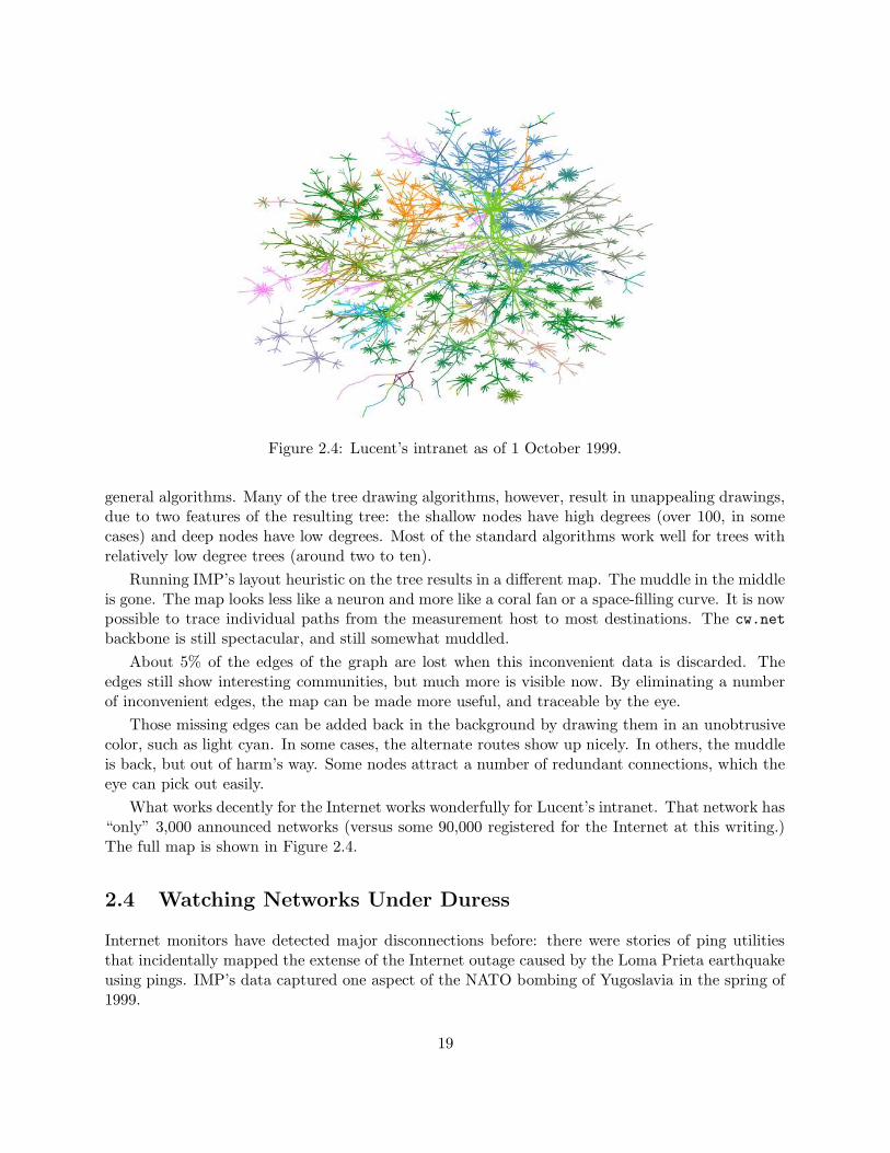
Figure 2.4: Lucent’s intranet as of 1 October 1999.

general algorithms. Many of the tree drawing algorithms, however, result in unappealing drawings,due to two features of the resulting tree: the shallow nodes have high degrees (over 100, in somecases) and deep nodes have low degrees. Most of the standard algorithms work well for trees withrelatively low degree trees (around two to ten).

Running IMP’s layout heuristic on the tree results in a different map. The muddle in the middleis gone. The map looks less like a neuron and more like a coral fan or a space-filling curve. It is nowpossible to trace individual paths from the measurement host to most destinations. The cw.net

backbone is still spectacular, and still somewhat muddled.

About 5% of the edges of the graph are lost when this inconvenient data is discarded. Theedges still show interesting communities, but much more is visible now. By eliminating a numberof inconvenient edges, the map can be made more useful, and traceable by the eye.

Those missing edges can be added back in the background by drawing them in an unobtrusivecolor, such as light cyan. In some cases, the alternate routes show up nicely. In others, the muddleis back, but out of harm’s way. Some nodes attract a number of redundant connections, which theeye can pick out easily.

What works decently for the Internet works wonderfully for Lucent’s intranet. That network has“only” 3,000 announced networks (versus some 90,000 registered for the Internet at this writing.)The full map is shown in Figure 2.4.

2.4 Watching Networks Under Duress

Internet monitors have detected major disconnections before: there were stories of ping utilitiesthat incidentally mapped the extense of the Internet outage caused by the Loma Prieta earthquakeusing pings. IMP’s data captured one aspect of the NATO bombing of Yugoslavia in the spring of1999.

19

0

10

20

30

40

50

60

70

80

90

04/08 04/22 05/06 05/20 06/03 06/17 07/01

Rou

ters

det

ecte

d

Date: mm/dd

Yugoslavia network during war

Figure 2.5: The number of reachable routers in the .yu domain over the course of the armedconflict.

During the first month of the war, few, if any, Internet links were cut. When, in early May,the bombing moved to the power grid, and the resulting disconnection is clearly shown in Figure2.5. The connectivity returned slowly. Incidentally, the reachable routes in neighboring Bosnia alsodeclined. One might infer (correctly) that Bosnia relies largely on the Yugoslavian power grid.

Figure 2.6 and Figure 2.7 compare May 2nd and May 3rd of the NATO bombing. It is interestingto note two large spiny “Koosh” balls in the upper right of the map have been significantly reduced.This would seem to imply that although the core routers at the center of the “Koosh” balls werenot directly damaged, many of the outlying routers were affected, possibly through power loss.

The maps also reveal that there appear to be only a few distinct routes into the Balkans fromthe measurement host. The power of the mapping technology is quickly apparent when viewing thelimited number of gateways that appear, showing the connectivity of Yugoslavian domains withthe rest of the Internet.

Measuring the network topology detected the results of distant damage in an semi-automatedway. It is unlikely that this is the first time such military uses have been considered. Relatedtechniques will doubtless be useful for monitoring the extent of other natural disasters, particularlyin well-connected parts of the world.

One of the largest difficulties with using such monitoring to examine events is that a smallfraction of the hosts on the Internet are affected. Thus, it is difficult to observe when consideringthe entire network. In this case, the set of hosts of interest was all the hosts in a country and nearbycountries. This is a relatively simple search to perform. If the set is all the hosts in a state or acity, this becomes more difficult. For example, measuring the effect of the terrorist attack on theWorld Trade Center would require finding hosts in the New York City and the area. Geolocation

20

05/02/1999

ches-netmapper.bell-labs.com204.178.16.1 (research.bell-labs.com.)

gr1-a3100s6.n54ny.ip.att.net.

204.70.10.146 (cw.net.)

core.Boston.cw.net.

mix1-fddi-0.Boston.cw.net.

public-enterprise-of-serbia.Boston.cw.net.

NISac-NET.telekom.yu.195.178.32.214 (odisej.telekom.yu.)

192.205.31.242 (mail.att.net.)p10-0-0.nyc1-br2.bbnplanet.net.

h1-0.nynap.bbnplanet.net.

Serial1-1-0.GW2.NYC2.ALTER.NET.

144.ATM2-0.XR1.NYC1.ALTER.NET.

Pennsauken1.NJ.US.EU.net.Nyk-nr01.NY.US.EU.net.

Nyk-cr02.NY.US.EU.net.

Asd-nr17.NL.EU.net.

Asd-nr05.NL.EU.net.Belgrade1.YU.EU.net.

routerban.elfak.ni.ac.yu.

195.ATM2-0.GW1.NYC5.ALTER.NET.

f1-0.pennsauken1.agis.net.

Belgrade2-S0.EUnet.yu.

295.ATM3-0.TR1.EWR1.ALTER.NET.

grafilrt.junis.ni.ac.yu.

ga013.philadelphia1.agis.net.

105.ATM4-0.TR1.DCA1.ALTER.NET.

195.ATM5-0.GW1.NYC5.ALTER.NET.

cisco1.rcub.bg.ac.yu.

412.ATM10-0-0.GW1.STK2.Alter.Net.299.ATM6-0.XR1.DCA1.ALTER.NET.

S111-asn-ns.telekom.yu.

Taide-gw.customer.ALTER.NET.

cisco-rmf.rcub.bg.ac.yu.

ga0113.washington7.agis.net.

IC-NET.telekom.yu.

router-siv1.sv.gov.yu.

NO-NIT-TN-0.taide.net.

NORD-NET.telekom.yu.

router3.junis.ni.ac.yu.

195.ATM11-0-0.GW1.DCA1.ALTER.NET.

321.ATM2-0.BR1.NYC5.ALTER.NET.

agis-bgp-local.loralorion.net.

194.247.193.49 (eunet.yu.)

seabone-gw.customer.ALTER.NET.

accs0.beotel.net.

loralorion-gw.customer.ALTER.NET.

meteo-gw.EUnet.yu.

YUBC-NET.telekom.yu.

bbanka-FR-W0-1M.beotel.net.

Partizan-NET.telekom.yu.

325.ATM1-0-0.CR1.STK2.Alter.Net.

TS-SC-2.net.yu.

421.ATM4-0.BR1.NYC5.ALTER.NET.

topas.meteo.yu.

frodo.yunord.net.

195.178.33.10 (odisej.telekom.yu.)

LI0007060.loralorion.net.

Belgrade5-E0.EUnet.yu.

komgrap-64k-yubc.yubc.net.160.99.1.109 (ban.junis.ni.ac.yu.)

atm-mi1-pa1.seabone.net.

router-siv3.sv.gov.yu.

LN-eth2.etf.bg.ac.yu.

debeli.ftn.ns.ac.yu.

RTS-NET.telekom.yu.

212.200.56.246 (yunord.net.)

eknrt.junis.ni.ac.yu.

Belgrade7-S0.EUnet.yu.

mirs-gw.EUnet.yu.YUNET-NET.telekom.yu.

ns2.www.yu.

tfrt.tf.bor.ac.yu.

leptir.cent.co.yu.

NS.InfoSky.yu.

d04-8000-su.yunord.net.

212.200.33.3

www.szi.sv.gov.yu.

amethyst.meteo.yu.

ns.cg.yu.

router4c.elfak.ni.ac.yu.

Figure 2.6: Map of paths to the Yugoslavian networks on May 2, colored by network.

05/03/1999

ches-netmapper.bell-labs.com204.178.16.1 (research.bell-labs.com.)

gr1-a3100s6.n54ny.ip.att.net.

br1-a3110s9.n54ny.ip.att.net.

newyork1.att-unisource.net.

amsterdam3.nl.att-unisource.net.

amsterdam5.nl.att-unisource.net.

192.205.31.242 (mail.att.net.)p10-0-0.nyc1-br2.bbnplanet.net.

h1-0.nynap.bbnplanet.net.

athens2.gr.att-unisource.net.att-unisource-gw.otenet.net.

athe-telecom-yu-peer.customers.otenet.gr.

Pennsauken1.NJ.US.EU.net.Nyk-nr01.NY.US.EU.net.

Nyk-cr02.NY.US.EU.net.

Asd-nr17.NL.EU.net.

144.ATM2-0.XR2.NYC1.ALTER.NET.

Asd-nr05.NL.EU.net.Belgrade1.YU.EU.net. NISac-NET.telekom.yu.

195.178.32.214 (odisej.telekom.yu.)

194.ATM3-0.GW1.NYC5.ALTER.NET.

144.ATM2-0.XR1.NYC1.ALTER.NET.

routerban.elfak.ni.ac.yu.

321.ATM2-0.BR1.NYC5.ALTER.NET.

f1-0.pennsauken1.agis.net.

295.ATM3-0.TR1.EWR1.ALTER.NET.

Belgrade2-S0.EUnet.yu.

ga013.philadelphia1.agis.net.

105.ATM4-0.TR1.DCA1.ALTER.NET.

311.ATM2-0-0.GW1.STK2.Alter.Net.

Taide-gw.customer.ALTER.NET.

299.ATM6-0.XR1.DCA1.ALTER.NET.

321.ATM2-0.BR2.NYC5.ALTER.NET.

ga0113.washington7.agis.net.

NO-NIT-TN-0.taide.net.

195.ATM11-0-0.GW1.DCA1.ALTER.NET.

194.ATM4-0.GW1.NYC5.ALTER.NET.

agis-bgp-local.loralorion.net.

meteo-gw.EUnet.yu.

195.178.33.110 (odisej.telekom.yu.)

loralorion-gw.customer.ALTER.NET.

IC-NET.telekom.yu.

194.247.193.49 (eunet.yu.)

Belgrade5-E0.EUnet.yu.

421.ATM4-0.BR1.NYC5.ALTER.NET.

TS-SC-2.net.yu.

LI0007060.loralorion.net.

topas.meteo.yu.

412.ATM10-0-0.GW1.STK2.Alter.Net.

S111-asn-ni.telekom.yu.

router0z.elfak.ni.ac.yu.

NS.InfoSky.yu.

router1c.elfak.ni.ac.yu.ns.b92.co.yu.

kapija.junis.ni.ac.yu.

router4c.elfak.ni.ac.yu.

cisco1.rcub.bg.ac.yu.

Belgrade7-S0.EUnet.yu.

amethyst.meteo.yu.

ns.cg.yu.

mirs-gw.EUnet.yu.

router2c.elfak.ni.ac.yu.

Figure 2.7: Map of the Yugoslavian Internet on May 3, colored by network. The main hubs in theupper right are still reachable, but they have lost a lot of leaves.

21

techniques should be able to address this problem, although they generally focus on the problemof determining the location of a host, rather than the opposite problem of determining the hostsand networks in an area.

2.5 Related Work

There are a number of Internet data collection and mapping projects underway. Some have beenrunning for a number of years, such as John Quarterman’s Matrix Information and DirectoryServices[63], which includes the “Internet weather report.” Martin Dodge has collected manyrepresentations of networks at Cybergeography[25]. Pansiot and Grad[70] mapped paths to 5,000destinations. The Mercator project at USC[42] tried to get a picture of the Internet at a giveninstance in time.

In terms of long-term mapping, k claffy and CAIDA are collecting a number of metrics fromthe Internet with skitter [61]. They have mapped the MBone, and collected path data to major websites. IMP is designed to map each known network, which maps to everything that exists, ratherthan everything that is used (i.e. the web servers). IMP’s goal is to discover every possible path,not just those in use.

Spring, Mahajan, and Wetherall’s Rocketfuel[94] focused on a single ISP. By focusing on oneISP at a time, they hoped to map it accurately and completely. Rocketfuel mapped from multiplelocations, using BGP tables to determine which paths go through the ISP of interest. Rocketfuelwas concerned with a snapshot, not daily measurement of the ISP.

Lyon’s Opte[59] attempts to measure the Internet in a single day. It is an amalgam of freely-available tools, combined together to produce a program to determine the topology of the Internet.Opte traces to each class C (/24) network, although it uses sampling techniques to discard allthe class C in a class B network, either because they are not used on the Internet or because theywould all result in the same path. Because it calls traceroute for each scan, Opte is computationallyexpensive (Opte reports a load of 60 during scanning) and difficult to control when compared toIMP, skitter, and Rocketfuel, which use traceroute tools specially written to run many traceroutesin parallel.

Internet maps are often laid out on the globe or other physical maps. The desire to map theInternet to geography is compelling, but it tends to end up with dense blobs of ink on NorthAmerica, Europe, and other well-connected regions3. However, connections to distant and moresparsely connected regions can be represented nicely, c.f. Quarterman’s map of connections toSouth America.

The problem with this method is the well-connected areas remain thoroughly inked, without aprayer of tracing paths through them. One approach is to simplify the map, showing connectionsby autonomous systems rather than individual routers. This is akin to showing the interstates onone map, and then creating local maps for each state. However, the AS connectivity graph is,proportionally, more connected than the IP graph. Thus, that graph is even more difficult to drawlegibly.

Interactive visualization tools can aid in navigating a database like ours. One can zoom, query,and browse at will. It is hard to see the entire net clearly on a screen: there are far too few pixels.

3Producing a map distorted based on Internet connectivity in order to alleviate this problem might be an interestingproblem for some cartographer.

22

However, H3Viewer[66, 67] is one tool that looks like a good start. It displays a spanning tree ofthe graph and allows the user both to navigate the tree and also view the non-tree edges.

2.6 Corporate Networks

The usefulness of network mapping is not limited to mapping the Internet. Corporate networksoften suffer from loosely-controlled growth, mergers, unauthorized connections, and general chaos.Network administrators are primarily concerned with making the network work properly. Whenfaced with a problem, their fix may result in unexpected changes to the network. As long as thechanges are not disruptive to the network, they can go undetected for long periods of time.

When IMP began, it was run from Bell Laboratories in Lucent Technology. Daily scans were runof Lucent’s network. The maps helped debug routing tables, which contained route announcementsfor networks like lsu.edu and the U.S. Postal Service. Although it is not clear if either LouisianaState University or the U.S. Postal Service were actually connected to the network, their CIDRblocks should not have appeared in the corporate routing tables.

The somewhat-surprising usefulness of the mapping and related technology resulted in Lucentforming a start-up venture to commercialize the technology. This venture, called Lumeta[58], spun-off of Lucent in October, 2000, taking the Internet Mapping Project with it. The commercializedversion of the software, with many features added, is offered as IPsonar by Lumeta.

One of the features added is the ability to display data using the graph layout. By coloringthe edges and nodes, the map can show insecure regions, new acquisitions, rare domains (domainswith few mapped hosts), unexpected networks, and many other forms of data. The data, andthe visualization there of, enables networks administrators to debug, optimize, and secure theircorporate networks.

2.7 Conclusion

The Internet maps, while seemingly less useful have certainly excited the media, who lacks goodvisuals of the Internet[10, 105]. From a less scientific standpoint, the maps are interesting to lookat, and one publisher created a poster out of it[73].

A number of researchers have picked up the routing database and run it through their visuali-zation tools or run graph-theoretic analyses of it, and at least one paper has resulted thus far[19].As the data collection began in August, 1998, it provides a good deal of information about routingfor a longer period of time than most routing studies to date have employed.

23

24

Chapter 3

IP Resolution1

Chapter 2 focused on the methodology used by the Internet Mapping Project[17] to measure thetopology of the Internet. There are several other ongoing projects to determine the IP-level topologyof the Internet[42, 61, 70, 94]. Although they vary in specifics, all of these projects use traceroute[46]to determine paths and then take the union of those paths to yield a topology. They all suffer fromthe same problem: IP aliasing.

IP aliasing is a result of how traceroute works. Recall that traceroute uses the source of ICMPerror messages to identify the hops along a path. The source of the messages is expressed as anIP address. Hosts, in particular routers, often have multiple IP addresses. If a host responds withdifferent IP addresses in different paths, then that host will appear multiple times in the topology.This behavior, known as IP aliasing, distorts the resulting topology. Routers commonly have oneIP address for each physical or virtual interface. Hosts may report any of their IP addresses as thesource IP address of traceroute responses[75]. Some hosts choose the responding IP address basedon the interface the packet came in, some on the interface the ICMP error message goes out, andsome always choose the same IP address. If a host exhibits either the first or second behavior, twotraceroutes passing through the host may contain different IP addresses.

IP aliasing distorts the produced topology in several ways. Adjacency is incorrect, as twoadjacent hosts with multiple IP addresses are often not adjacent for all pairs of IP addressesbelonging to those hosts. This causes hosts to be farther apart in the topology than they are inreality. IP aliasing also distorts distributions in a measured topology. It obviously inflates the sizeof the topology, increasing the number of hosts and links. Because hosts are farther apart in thetopology, distance distributions are also affected. Degree distribution is also distorted, although itis more difficult to determine the net effect of IP aliasing on degree distributions.

In addition to distorting the topology, IP aliasing also makes it difficult to determine whethertwo paths are the same. Analyzing path symmetry and route stability requires determining if twopaths are the same. If two paths differ only in the selection of the IP addresses that represent thehops, the paths are considered different, despite the fact that they describe the same path withinthe network. Without correcting for IP aliasing, any measurements of path symmetry or routestability understates the true behavior of the network.

1This chapter represents work originally published as “Eliminating Machine Duplicity in Traceroute-based InternetTopology Measurements” as a technical report at Carnegie Mellon University[6].

25

The problem of determining the set of IP addresses belonging to a host is known as the IP aliasresolution problem. Although IP alias resolution is not a new problem, previous work was focusedon producing a topology. The bulk of the focus was on minimizing the number of links and routersnot included in the topology. Little effort was made to analyze the IP alias resolution techniqueused, much less to compare it against other possible techniques.

This chapter considers several techniques for IP alias resolution. There are three major knowntechniques for detecting IP aliasing: UDP, IPid and rate limitation. The UDP technique is theoldest approach, first proposed by Pansiot and Grad[70]. This approach looks at the source ad-dress of ICMP Port Unreachable responses to UDP packets. It was also used by Govindan andTangmunarunkit[42], Barford, et al.[3], and Keys[52]. The IPid technique looks for correlated be-havior in the IP identification field of the IP header[76]. It was used by Spring, et al.[94]. Therate limitation technique looks for correlation in rate limitation behavior between IP addresses.Although the rate limitation technique was briefly mentioned by Spring, et al.[94], they rarelyemployed it.

This chapter presents algorithms embodying each technique, analyzing its efficacy, and comparesthe presented algorithms with each other and with some previous algorithms. Specific algorithmsare designed to work on large sets of IP addresses. Two methods are presented to divide the inputset into smaller sets: TTL and adjacency. Splitting algorithms employing these splitting methodsreduce the number of packets required by IP alias resolution algorithms, but may discard validpairs of IP addresses. The efficacy of each technique and algorithm is analyzed in four dimensions:cost, coverage, accuracy, and unique coverage. Cost is defined by the number of packets sentand the amount of time taken to test a set of approximately 400,000 IP addresses. Coverage is thecompleteness of the output. Accuracy is derived from the number of pairs of IP addresses belongingto different hosts that are labeled as belonging to the same host. Unique coverage is how much thetechnique finds that is not found by any other technique or algorithm.

Section 3.1 gives the details of the experimental setup and methodology. Section 3.2 explains thesplitting methods and algorithms, while section 3.3, 3.4, and 3.5 give the specific IP alias resolutionalgorithms. Section 3.6 lists the results of the experiments, and section 3.7 presents conclusions.

3.1 Methodology

Before giving algorithms, the requirements of an IP alias resolution algorithm, including inputs andoutputs, must be defined. The input to an IP alias resolution algorithm is a set of IP addressesof interest. An algorithm can send packets of any type to any set of IP addresses in any order.The output of an algorithm is a set of pairs of IP addresses, where the IP addresses in a pair arebelieved to belong to the same host. The output may contain IP addresses not within the originalset of IP addresses. An IP address may appear in multiple pairs, allowing the algorithm to expressthe belief that a host has three or more IP addresses.

It is often useful to have disjoint groups of IP addresses, where each group represents the IPaddresses believed to belong to one host. The set of pairs can be mathematically transformedto disjoint groups by taking the equivalence classes of the transitive closure of the equivalencerelationship implied by the pairs. Algorithmically, this can be done starting with each IP addressin a group by itself. For each pair, combine the groups containing the two IP addresses of the pair,if the two IP addresses are not already in the same group. This process yields the desired disjoint

26

groups. Note that this process creates new pairs of IP addresses believed to belong to the samehost that were not in the original set. This will discussed in Section 3.6.

One use of these disjoint groups is refining the network topology resulting from traceroutemeasurements. This is done by collapsing the IP addresses believed to belong to the same host toa single node. After this combination, the graph is reduced to a simple graph again by removingboth self-loops and duplicate instances of edges.

For an algorithm to be accurate, it must have minimal effect on the network. There are twoways an algorithm could affect the network: technical and political. If an algorithm causes thenetwork to rebalance load or deal with host or link failure, the output will be incorrect. If analgorithm causes network operators to become upset and block the measurement host, the outputwill also be flawed. The effect on a network is difficult to quantify in general. Because all methods,techniques, and algorithms herein employ high-port UDP packets, the effect can be quantified bythe packet rate and the length of time the algorithm runs.

An IP alias resolution algorithm should send no more than 2,000 packets per second. A packetrate of 2,000 packets per second corresponds to 60% of an T1. This means that the algorithm isunable to overload any T1 lines in the network. Moreover, the technique is usable from measurementhosts that have only T1-speed connectivity. This bound on connection speed means that almostanyone can use the algorithms.

The time limit for the algorithms to run was selected as one day for an input set of 400,000IP addresses. The input set limitation is required to analyze runtime. An input set of 400,000 IPaddresses represents roughly two and a half times the number of router IP addresses found eachday by the Internet Mapping Project[18]. Thus, it should be sufficient for most purposes. Limitingthe run time mitigates several issues.

Firstly, the output of the algorithm attempts to characterize the network over the entire mea-surement time. Long time limits mean that the algorithm is trying to characterize a dynamicnetwork over a long time with a single output. Few configuration changes resulting in backbonerouter migrating between IP addresses are made on an average day. Thus, this time limit ensuresthat the network is mostly static over the measured time period.

Secondly, for an algorithm to work on a pair of IP addresses, the corresponding host must beon for the entire run of the algorithm configured with that pair of IP addresses. Requiring analgorithm to run in less than one day limits the amount of network downtime confounding thealgorithm.

Thirdly, the longer an algorithm runs, the more packets it may send and the more likely it is toannoy a network operator. The limit of one day and 2,000 packets means that no more than 172.8million packets (10 gigabytes) are sent, or 432 packets (25 kilobytes) per IP address. In practice,the actual values are much lower, but even 432 packets over a day to an IP addresses should haveminimal effect on the host.

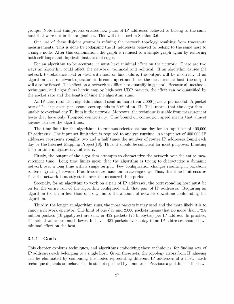
3.1.1 Goals

This chapter explores techniques, and algorithms embodying those techniques, for finding sets ofIP addresses each belonging to a single host. Given these sets, the topology errors from IP aliasingcan be eliminated by combining the nodes representing different IP addresses of a host. Eachtechnique depends on behavior of hosts not specified by standards. Previous algorithms either have

27

poor accuracy or require packet counts that are quadratic in the number of IP addresses to betested. For a sending rate of 2,000 packets per second (approximately T1 speeds), testing 1,000 IPaddresses using an algorithm that sends two packets for each pair would take a little more thaneight minutes, which is reasonable. However, it does not scale to testing all IP addresses of routerson the public Internet. This chapter uses a set of 380,000 such IP addresses, which would takeover two years to test. Although higher packet rates would decrease the amount of time required,quadratic algorithms obviously scale poorly to large data sets. The goal is to obtain scalabilitywhile minimizing the reduction in accuracy. This chapter presents specific ways to test for IPaliasing on Internet scale using a reasonable number of packets in a reasonable time period.

3.1.2 Experimental Setup

All experiments were done over a T1 connection connected via UUNet. As mentioned above, thepacket rate limitation mentioned above of 2,000 packets per second represents about 60% of aT1, as replies to the test packets contain 56 bytes. The total utilization of the local T1 was keptunder 85%. This means there was not significant local packet loss, which would affect both theexperiments herein and other local traffic.

The input set of IP addresses came from hops within 77 days of traceroute data from theInternet Mapping Project[18]. After discarding unroutable and private address space, the originalinput set consisted of 587,828 IP addresses, although only 386,157 were found to be responsive toUDP packets. The traceroutes were daily runs from May 2002 to July 2002, consisting of about240,000 individual traces per run. This input set was selected as both representative and rich in IPaliasing. The goal is to improve topology measurements based on traceroute, which is exactly thesource of the IP addresses. Moreover, many hosts were expected to appear multiple times underdifferent IP addresses due to route changes between days.

The fact that only 66% of the IP addresses responded to UDP packets was surprising. Thisis a result of the traceroutes from which the IP addresses came employing ICMP Echo Requestpackets, not UDP packets. 92% of the IP addresses were responsive to ICMP Echo Requests. Thus,most (76%) of the IP addresses that failed to respond to the UDP packets were either behind afirewall that blocked the UDP packets but not the ICMP Echo Request packets or were configuredto respond to ICMP Echo Request packets but not UDP packets. The other 24% of the non-responders (8% of all the IP addresses tested) did not respond for some other reason, such as beingturned off, being retired, losing connectivity, or routers that forward packets but cannot, either dueto firewalls or residing on unannounced networks, be directly addressed.

3.1.3 Packet Collection

From the responsiveness results, it would be desirable to use ICMP packets to test. However, allpresented algorithms use UDP probe packets to attempt to elicit ICMP port unreachable responses.This is a coincidence, not a design constraint. ICMP Echo Request packets are generally treateddifferently than UDP packets. This is partly because line cards often respond to ICMP packets,rather than the router itself. The specific reason why ICMP Echo Request packets will not work foreach method and technique will be given later. Using TCP packets would be more invasive to themeasured systems, probably perform worse, and introduce additional complexity by introducingnew response types to address.

28

When collecting responses to packets sent to a large set of IP addresses, there are two com-plicating features. First, responses must be matched with requests. As UDP packets elicit ICMPport unreachable responses, which have a partial copy of the original packet within them, this doesnot seem especially difficult. Unfortunately, the destination listed within the packet enclosed in theresponse is not always the same as the destination of the original probe packet. One cause of thisbehavior is improper or incomplete network address translation (NAT). Because of this, matchingis done using the destination port in the original UDP packet.

The second problem is that not all packets elicit responses. Non-response can be caused byrouting problems, packet loss, response rate limits, firewalls, and hosts being disconnected from thenetwork. Thus, the packet collection algorithm must make multiple attempts in order to obtainreliable response rates.

Algorithm 3.1:

1. Let S be the set of IP addresses

2. Send a packet to every IP address in S

3. Output R, the responses collected from step 2

4. If ‖R‖ < 1

3‖S‖ then exit

5. Remove all IP addresses of S which yielded a response in R

6. Goto step 2

As shown as Algorithm 3.1, the packet collection algorithm works in passes. Each pass testsevery IP address for which the algorithm does not yet have a response. Passes continue until somepass obtains responses from less than a third of the IP addresses tested. This algorithm gives overa 93% response rate (median and mean of seven runs), with 83% of the IP addresses being reliableresponders (responding to seven of seven runs). This algorithm will not obtain responses from IPaddresses that have long-term (minutes) reasons to not respond, such as firewalls. It will obtainresponses from most IP addresses with packet loss, rate limits, and transient routing problems.

3.2 Splitting Methods

Splitting is the process of dividing the input into smaller sets that can be tested independently.Reducing the set size makes quadratic IP alias resolutions algorithms run more efficiently. Theidea is to decrease the size of the sets with a small amount of effort. While some IP addresses mayappear in multiple sets, the total number of pairs of IP addresses to test should be less than thenumber of pairs from the original set. Two methods to split sets of IP addresses were employed:TTL splitting and adjacency splitting.

DNS splitting, used by RocketFuel[94], uses DNS names to divide the set. DNS methods aredependent on knowledge of DNS naming schemes and are sensitive to naming errors[95]. As such,they can be nearly-infinitely improved by adding knowledge of more autonomous systems. Thismakes analyzing a particular DNS splitting method nearly meaningless.

Kohno, Broido, and Claffy[54] propose using clock skews to detect multiple IP addresses belong-ing to the same host. Their work involves sending many packets to each address to determine clockskew, making it impractical for more than a few hundred hosts. However, it may be reasonable touse less accurate techniques to divide the set. This was not explored.

29

0

0.01

0.02

0.03

0.04

0.05

0.06

0.07

0.08

0.09

0 32 64 96 128 160 192 224 256

Fra

ctio

n of

Res

pons

es w

ith th

at T

TL

Time to Live

Figure 3.1: Observed distribution of TTL values for packets from 380,000 IP addresses.

3.2.1 TTL Method

TTL splitting uses the eight-bit “Time to Live” (TTL) field from the IP header. This field isdecremented by one for each hop a packet traverses. If the field reaches zero before the packetreaches its destination, the packet is discarded and an error message may be returned to the sourceof the packet. This insures that packets on the Internet have limited lifetime.

Hosts initialize the value of the TTL independent of the destination of the packet. Moreover,most hosts decide which interface to send out a response packet based on the destination withoutregard to which interface received the original packet. It follows from these two behaviors thatsending packets to two IP addresses of such a host will result in two response packets with thesame TTL. If sending packets to two IP addresses results in response packets with different TTLs,the two IP addresses do not belong to the same host.

TTL values are dependent on two values: (a) initial TTL selection and (b) length, in hops, ofthe path from the IP address to the measurement host. Because few initial TTL values are used inpractice, IP addresses in the same TTL-value bucket are, for the most part, the same distance fromthe measurement host. Thus, TTL splitting roughly divides the IP addresses into groups based onthe length of the path from the IP addresses to the measurement host. This is exploited further inChapter 4.

Algorithm 3.2:

1. Use Algorithm 3.1 to collect responses from each IP address

2. Discard any IP address that does not respond

3. For each value, output a group containing IP addresses whose response had that TTL value

One problem with this approach is that routes may change in the middle of an experimentalrun. Thus, TTLs coming from the same host may differ, either due to a true routing change or loadbalancing. Fortunately, load balancing over paths of different lengths is unusual and most routesare static over reasonable time spans (minutes to hours)[72].

A larger problem with this technique is that the TTL field has only 255 possible values, andthe distribution is highly skewed, as show in Figure 3.1. Initial TTL values are not distributed

30

2

(b)

(a)

(c)

A

B

B

A

B

1

1

1

1

1

A2

A

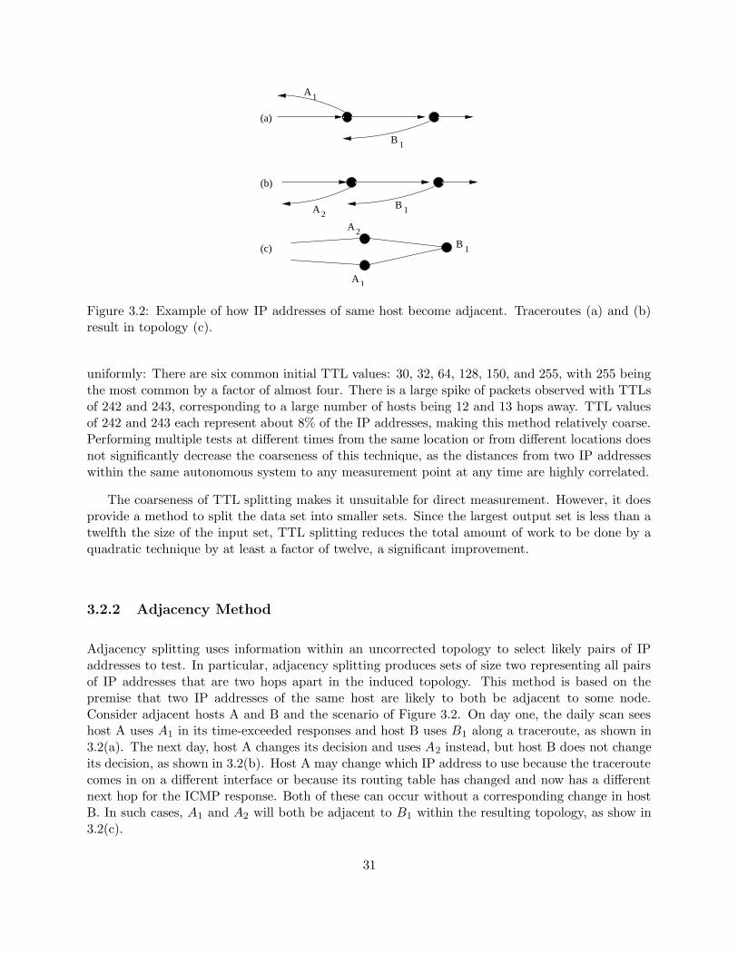
Figure 3.2: Example of how IP addresses of same host become adjacent. Traceroutes (a) and (b)result in topology (c).

uniformly: There are six common initial TTL values: 30, 32, 64, 128, 150, and 255, with 255 beingthe most common by a factor of almost four. There is a large spike of packets observed with TTLsof 242 and 243, corresponding to a large number of hosts being 12 and 13 hops away. TTL valuesof 242 and 243 each represent about 8% of the IP addresses, making this method relatively coarse.Performing multiple tests at different times from the same location or from different locations doesnot significantly decrease the coarseness of this technique, as the distances from two IP addresseswithin the same autonomous system to any measurement point at any time are highly correlated.

The coarseness of TTL splitting makes it unsuitable for direct measurement. However, it doesprovide a method to split the data set into smaller sets. Since the largest output set is less than atwelfth the size of the input set, TTL splitting reduces the total amount of work to be done by aquadratic technique by at least a factor of twelve, a significant improvement.

3.2.2 Adjacency Method

Adjacency splitting uses information within an uncorrected topology to select likely pairs of IPaddresses to test. In particular, adjacency splitting produces sets of size two representing all pairsof IP addresses that are two hops apart in the induced topology. This method is based on thepremise that two IP addresses of the same host are likely to both be adjacent to some node.Consider adjacent hosts A and B and the scenario of Figure 3.2. On day one, the daily scan seeshost A uses A1 in its time-exceeded responses and host B uses B1 along a traceroute, as shown in3.2(a). The next day, host A changes its decision and uses A2 instead, but host B does not changeits decision, as shown in 3.2(b). Host A may change which IP address to use because the traceroutecomes in on a different interface or because its routing table has changed and now has a differentnext hop for the ICMP response. Both of these can occur without a corresponding change in hostB. In such cases, A1 and A2 will both be adjacent to B1 within the resulting topology, as show in3.2(c).

31

Algorithm 3.3:

1. Let S = ∅

2. For each IP address A in the topology

(a) For each pair of IP addresses B and C adjacent to A in the topology, add (B,C) to S.

3. Remove duplicate pairs from S

4. Output S

The obvious algorithm would be to create a set for each IP address consisting of all IP addressesadjacent to that IP address. However, some pairs of IP addresses appear in many such sets, whichwould result in testing those pairs many times. To avoid this problem, the algorithm, shown asAlgorithm 3.3, outputs all pairs of IP addresses that share an adjacent IP address.

The data collection required to obtain the topology is not considered. IP alias resolution ismost commonly used to fix topology measurements. Because the data collection required to obtaina topology is done in most cases where this algorithm would be used, that data collection is notcounted as part of the cost of this algorithm.

The scenario that makes two IP addresses of a host adjacent to some IP address is less commonthan the scenario for TTL equality. As such, this method is expected to have worse coverage thanTTL splitting. The major advantage of this method is that the number of pairs to test is nearlylinear in the number of IP addresses in the input set, making it a useful splitting algorithm fortechniques that scale poorly.

3.3 UDP Technique

The problem of IP aliasing was first observed by Pansiot and Grad when mapping multicasttrees[70]. Their techniques for IP alias resolution sent UDP packets to non-listening ports to findpairs of IP addresses belonging to the same host. When they sent a UDP packet to a port wherethey did not expect a service to be listening, hosts receiving these packets responded with ICMPunreachables, specifically port unreachable. Pansiot and Grad noted that the source IP address ofthe ICMP error packet was not always the same as the destination of the UDP packet. As it isunlikely that a different host would respond with an UDP port unreachable than the destinationof the UDP packet, they used such responses as evidence that the source of the ICMP error packetand the destination of the UDP packet were the same host.

This technique is nice in that it requires sending only one packet to each IP address in the inputset. Because this technique scales well, it requires no splitting. Many hosts pick the source of theICMP error packet as the IP address of the outbound interface, making the address constant overall interfaces. This technique will not work on hosts that select the source of the response packetto be the original destination. A priori, it is not clear what the relative prevalence of these twotypes of hosts is on the Internet.

The specific algorithm used is relatively straight-forward:

32

Algorithm 3.4:

1. Use Algorithm 3.1 to collect responses from each IP address

2. Discard responses from 0.0.0.0, the measurement host’s IP addresses, and private IP addresses.

3. Discard responses which list a different original destination IP address than expected.

4. Group IP addresses by the source IP addresses listed in the responses

This technique is, by far, the most commonly used approach. Govindan and Tangmunarunkit[42]used a more complicated form of this technique that uses multiple packets and source routing[76].Barford, et al.[3] used the UDP technique, although without the additional features of Govindanand Tangmunarunkit. iffinder[52], written by Keys uses several techniques for finding interfaces,but its most successful technique is the UDP technique.

The popularity of the UDP technique is partially due to both its simplicity and speed: onlyone packet needs to be sent for each IP address, ignoring retries of the packet collection algorithm.This technique cannot benefit from splitting methods, but it does not need them either.

False positives in this technique are caused by hosts responding with IP addresses that are notuniquely their own. This is most obvious when they use invalid IP addresses that are clearly nottheir own or when they use private IP addresses, which can be used multiple times within thenetwork. The algorithm discards these obvious errors, but some hosts respond with IP address notuniquely their own that are not detected by the algorithm due to operating system peculiarities orsystem defaults.

3.4 IPid Technique

A different IP alias resolution technique, employed by RocketFuel[94], uses the IP identificationfield as a bucketing technique to detect multiple IP addresses belonging to the same host. Manyhosts set this 16-bit header field using a global counter that is incremented by one for each packetsent. If such a host responds to two packets at approximately the same time, it will send packetswith similar IPid values, even if the packets are sent to two different IP addresses of the host.Spring, et al. designed the RocketFuel algorithm to work on small data sets, as they were focusedon determining the connectivity of only one ISP at a time. The presented algorithm is designedfor larger data sets and includes an improved verification algorithm. The presented algorithm ismathematically compared with RocketFuel.

The IPid field provides a natural way to verify that two IP addresses belong to the same host,as the value of the IPid field within responses from the two IP addresses of the same host will besimilar. Discovering pairs of IP addresses belonging to the same host is a bit more difficult. Here,packets must be sent to a large number of IP addresses and the IPid field values in the responsesexamined to determine which IP addresses may belong to the same host. For large input sets, it isdifficult to detect if the first and last IP address belong to the same host.

Assume both the IPid change rates for two IP addresses probed t seconds apart are both belowR, but the change rates are not known. Without loss of generality, presume the IPid of the firstresponse is 0 and the IPid of the second response is d. The two IP addresses may belong to thesame host if d < Rt. If initial IPid values are random and the two IP addresses are not the samehost, this happens with probability Rt

65536.

33

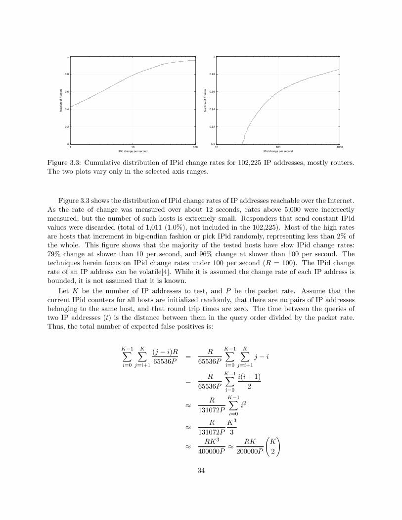
0

0.2

0.4

0.6

0.8

1

1 10 100

Fra

ctio

n of

Rou

ters

IPid change per second

0.9

0.92

0.94

0.96

0.98

1

10 100 1000

Fra

ctio

n of

Rou

ters

IPid change per second

Figure 3.3: Cumulative distribution of IPid change rates for 102,225 IP addresses, mostly routers.The two plots vary only in the selected axis ranges.

Figure 3.3 shows the distribution of IPid change rates of IP addresses reachable over the Internet.As the rate of change was measured over about 12 seconds, rates above 5,000 were incorrectlymeasured, but the number of such hosts is extremely small. Responders that send constant IPidvalues were discarded (total of 1,011 (1.0%), not included in the 102,225). Most of the high ratesare hosts that increment in big-endian fashion or pick IPid randomly, representing less than 2% ofthe whole. This figure shows that the majority of the tested hosts have slow IPid change rates:79% change at slower than 10 per second, and 96% change at slower than 100 per second. Thetechniques herein focus on IPid change rates under 100 per second (R = 100). The IPid changerate of an IP address can be volatile[4]. While it is assumed the change rate of each IP address isbounded, it is not assumed that it is known.

Let K be the number of IP addresses to test, and P be the packet rate. Assume that thecurrent IPid counters for all hosts are initialized randomly, that there are no pairs of IP addressesbelonging to the same host, and that round trip times are zero. The time between the queries oftwo IP addresses (t) is the distance between them in the query order divided by the packet rate.Thus, the total number of expected false positives is:

K−1∑

i=0

K∑

j=i+1

(j − i)R

65536P=

R

65536P

K−1∑

i=0

K∑

j=i+1

j − i

=R

65536P

K−1∑

i=0

i(i + 1)

2

≈R

131072P

K−1∑

i=0

i2

≈R

131072P

K3

3

≈RK3

400000P≈

RK

200000P

(

K

2

)

34

Note that this formula only works when RK65536P

< 1, since otherwise a host’s IPid counter mayroll-over within the testing window.

In practical terms, if R = 100, K = 400, 000, and P = 2, 000, the formula states that there willbe 8 billion false positives, 10% of all pairs. Thus, algorithms based on this technique need eithermultiple phases or splitting methods if they are to work on large input sets. The algorithm belowdoes both.

3.4.1 Algorithm with TTL Splitting

The algorithm has four phases: TTL splitting (Algorithm 3.2), IPid splitting, IPid testing, andIPid verification.

IPid splitting

Algorithm 3.5:

1. Let G be the set of sets of IP addresses from TTL splitting

2. Let S ∈ G; remove S from G

3. Let R = 100, the maximum IPid change rate supported

4. Use Algorithm 3.1 to collect a packet from each IP address in S

5. Let t be the time taken to collect packets

6. Let S = {Aj}. Let dj be the IPid received from IP address Aj

7. Let N =⌊

65536

tR

⌋

, the number of sets to produce

8. For each 0 ≤ i ≤ N − 1,

(a) Let Si ={

Aj |⌊

Ndj

65536

⌋

≡ {i, i + 1}(mod N)}

(b) if ‖Si‖ ≤ 2000, output Si

(c) Otherwise, add Si to G

9. If G 6= ∅, goto Step 2

IPid splitting, shown as Algorithm 3.5, divides the TTL-split groups into groups with 2,000 orfewer IP addresses to simplify later testing. It sends packets to each IP address and collects theIPid of the response. The IPid range 0-65,535 is split into subranges based on the maximum IPidchange rate supported (R) and the time it took to collect the packets. The size of the range is theproduct of the maximum rate and the collection time (with round-off distributed roughly evenlyacross groups). A group consists of all IP addresses with IPid values within a range and the nextrange (for the highest range group, the next range is the first range). This means that every IPaddress that responded is in two groups.

Presuming that the host did not change at an average rate exceeding the maximum supportedrate and the host responded for all IP addresses, every pair of IP addresses belonging to that hostexists in some group. In particular, the first responding IP address of each pair is put into a groupcontaining the last responding IP address. If a resulting group has more than 2,000 IP addresses,the process is repeated on that group. In order to decrease the size of the largest group, at leastthree groups must be created. Therefore, the number of IP addresses within a single test groupcannot exceed 65536P

3R≈ 21845P

R, where P is the average rate of packet transmission and R is the

35

maximum supported IPid change rate. For the experimental results given, R = 100 and P ≈ 2000,which means the groups inputted into this phase cannot exceed 436,900 IP addresses. Although theinput set could be run directly (barely), running TTL splitting first greatly decreases the amountof duplication of IP addresses done by IPid splitting.

IPid testing

Algorithm 3.6:

1. Let R = 100, the maximum IPid change rate supported

2. Let S be an input set

3. Use Algorithm 3.1 to collect a packet from each IP address in S

4. Wait at least five minutes

5. Use Algorithm 3.1 to again collect a packet from each IP address in S

6. Let ∆1 = Rt1, where t1 is the time taken to collect the packets the first time

7. Let ∆2 = Rt2, where t2 is the time taken to collect the packets the second time

8. Let S = {Aj}. Let dkj be the IPid received from IP address Aj on the kth run (k ∈ {1, 2})

9. Output {{Ai, Aj}| ‖d1j − d1

i ‖ ≤ ∆1 and ‖d2j − d2

i ‖ ≤ ∆2}.

IPid testing, shown as Algorithm 3.6, takes sets of 2,000 or fewer IP addresses and proposespairs of IP addresses that may be aliases of each other. Packets are sent to every IP address andthe IPid of the responses are collected. Pairs of IPid values are then examined to determine if theyare consistent with a host whose IPid counter is changing no faster than the supported rate, withthe assumption that the reverse path delays do not exceed 200 milliseconds (this allows for a gooddeal of jitter). Pairs of IP addresses that meet this criteria are outputted. From the equation inthe previous section, the percentage of false positives would be expected to be quite low. However,this ignores the fact that this phase is dependent on the previous splitting work, since 40% of thehosts have IPid values that change at a rate slower than 1 per second (see Figure 3.3). Due to thenumber of false positives, IPid testing is done twice on each set with at least five minutes betweenpairs and only pairs that appear in both tests of a set are considered. In practice, the first roundof packet collection is done for each set. When all sets have been tested once, they are then testedagain. This avoids spending five minutes per set sending no packets.

IPid verification

IPid verification tests pairs of IP addresses to determine if they belong to the same host. IPidverification is done in groups of 2,000 pairs such that no IP address appears in two pairs. To testa pair, packets are sent to the first IP address, then to the second, then to the first, and then tothe second, with a one second delay between each packet sent to a single pair. The IPid values ofthe responses must be consistent with the assumption that the host responding to both addressesdoes not change its IPid quickly. In particular, the IPid of the responses must be monotonicallyincreasing and separated by no more than 400. This interlacing ensures that regardless of the initialvalues, the pair will be discarded if the hosts’ IPid values are not moving at similar rates. For IPaddresses with slowly-changing IPid values, pairs with similar initial IPid values (most of the falsepairs tested), the interlacing is likely to reveal two responses with the same IPid value.

36

IPid verification, shown as Algorithm 3.7, has four possible results for each pair: accept, re-jection, failure (did not receive responses to all packets), and skipped (could not find a test setto add the pair to that did not already contain one of the IP addresses of the pair). Verificationsweeps are done through the incomplete (not accepted or rejected yet) pairs until at least half of thenon-decisions are failures, at which point the remaining unvalidated pairs are considered rejected.

Algorithm 3.7:

1. Let G = {pi} be the input set, where pi are pairs.

2. Let ∆ = 400

3. Set S = ∅

4. If ‖S‖ = 2000 or G = ∅,

(a) Set the packet rate to ‖S‖ packets per second

(b) Output a packet to the first IP address of each pair in S

(c) Output a packet to the second IP address of each pair in S

(d) Repeat Steps 4b and 4c

(e) For each pair p ∈ S,

i. If pair p did not get four responses, mark p as Failed and consider the next pair

ii. If d2 − d1 mod 65536 > ∆ mark p as Rejected

iii. If d3 − d2 mod 65536 > ∆ mark p as Rejected

iv. If d4 − d3 mod 65536 > ∆ mark p as Rejected

v. If p has no mark, mark p as Accepted

(f) Set S = ∅

5. If G = ∅, exit

6. Let p ∈ G be a pair of IP addresses randomly selected from the pairs of G.

7. If either IP address of p is in some pair in S, mark p as Skipped and goto step 4

8. Otherwise, add p to S and goto step 4

3.4.2 Algorithm with Adjacency Splitting

The second IPid algorithm employs adjacency splitting instead of TTL splitting. The algorithmperforms adjacency splitting and runs IPid verification on the resulting pairs.

3.4.3 Discussion

Figure 3.4 compares the IPid verification algorithm to RocketFuel’s algorithm[94]. To compare IPaddresses A and B, RocketFuel sends packets to A, then to B, and then to A again. It then checksif the response from B has an IPid that is between the two responses from A and that the IPidresponse from B is within 200 of the IPid response of A. The IPid verification algorithm here sendsa fourth packet to B, with the additional constraint that the second response from A must have anIPid that is between the two responses from B.

IPid verification’s false positive rate is much better than RocketFuel’s. Assuming constant IPidrate change, random IPid starting values, and the distribution of IPid rate changes shown in Figure3.3, the probability of both RocketFuel conditions holding true for a false pair of IP addresses is

37

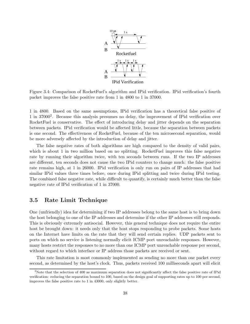
µ

AB

AB

IPid Verification

Rocketfuel1 s 1 s1 s

1 s10 s

Figure 3.4: Comparison of RocketFuel’s algorithm and IPid verification. IPid verification’s fourthpacket improves the false positive rate from 1 in 4800 to 1 in 37000.

1 in 4800. Based on the same assumptions, IPid verification has a theoretical false positive of1 in 370002. Because this analysis presumes no delay, the improvement of IPid verification overRocketFuel is conservative. The effect of introducing delay and jitter depends on the separationbetween packets. IPid verification would be affected little, because the separation between packetsis one second. The effectiveness of RocketFuel, because of the ten microsecond separation, wouldbe more adversely affected by the introduction of delay and jitter.

The false negative rates of both algorithms are high compared to the density of valid pairs,which is about 1 in two million based on no splitting. RocketFuel improves this false negativerate by running their algorithm twice, with ten seconds between runs. If the two IP addressesare different, ten seconds does not cause the two IPid counters to change much: the false positiverate remains high, at 1 in 26000. IPid verification is only run on pairs of IP addresses that hadsimilar IPid values three times before, once during IPid splitting and twice during IPid testing.The combined false negative rate, while difficult to quantify, is certainly much better than the falsenegative rate of IPid verification of 1 in 37000.

3.5 Rate Limit Technique

One (unfriendly) idea for determining if two IP addresses belong to the same host is to bring downthe host belonging to one of the IP addresses and determine if the other IP addresses still responds.This is obviously extremely antisocial. However, this general technique does not require the entirehost be brought down: it needs only that the host stops responding to probe packets. Some hostson the Internet have limits on the rate that they will send certain replies. UDP packets sent toports on which no service is listening normally elicit ICMP port unreachable responses. However,many hosts restrict the responses to no more than one ICMP port unreachable response per second,without regard to which interface or IP address those packets are received or sent.

This rate limitation is most commonly implemented as sending no more than one packet everysecond, as determined by the host’s clock. Thus, packets received 100 milliseconds apart will elicit

2Note that the selection of 400 as maximum separation does not significantly affect the false positive rate of IPidverification: reducing the separation bound to 100, based on the design goal of supporting rates up to 100 per second,improves the false positive rate to 1 in 43000, only slightly better.

38

Description IP Count Pct.

Tested 386,157 100.0%

Five responses 139,133 36.0%

Two to four responses 10,668 2.8%

One response 227,368 58.9%

No valid response 8,988 2.3%

Figure 3.5: Summary of rate limitation test of sending five packets to each IP address.

1200 msec

150 msec

BA

Figure 3.6: Rate limitation algorithm.

a response only if the clock ticks (increments the second counter) between receiving the packets,which would occur 10% of the time. This implies a technique by which it can be determined iftwo IP addresses belong to the same host. Because the clock ticks occurs at an unknown time,such a technique technique must do multiple experiments to avoid being fooled by a clock tick anddrawing the false conclusion that the two IP addresses do not belong to the same host.

To determine how frequent this rate limitation is in practice, five UDP packets were sent inquick succession to each of the 386,157 IP addresses: five packets to the first IP address, five tothe second, etc. Multiple responses to the same packet were ignored. Figure 3.5 summarizes theresults. Three-fifths of the IP addresses rate-limit their responses and should be responsive to thistechnique.

This technique is time-sensitive. Sending two packets to different addresses separated by threeseconds yields no information to this technique, as the clock will tick between the times at whichthe packets are received. Thus, splitting is necessary if the number of IP addresses to test exceedsthe packet rate. The naıve method would be to create test sets of 1,000 IP addresses each suchthat every pair of IP addresses share membership to some test set. It would take more than morethan 160,000 sets to do this for 400,000 IP addresses. Presuming three seconds a set, it would takemore than nine days to run one pass. The rate limitation technique is sensitive to timing errors andpacket loss. Its error rate means that multiple passes are necessary to obtain meaningful results. Ifthree passes on the entire input set must be done, the naıve algorithm would take 27 days. UsingTTL splitting would reduce the process to about 41 hours, still too long. Thus, adjacency splittingwas employed to be able to test the set within a day.

39

3.5.1 Algorithm

Algorithm 3.8:

1. Let G be the set of pairs from adjacency splitting

2. Send five packets to each IP address (five to first IP, then five to second, etc).

3. Discard the pairs of G with either IP address responding to all five packets

4. For each pair p ∈ G left,

(a) Let p = {a, b} be a pair of IP addresses from adjacency splitting

(b) Send packet to a, wait 150 milliseconds, send packet to b

(c) Wait 1050 milliseconds

(d) Send packet to b, wait 150 milliseconds, send packet to a

(e) If four packets received, mark p as Rejected

(f) Otherwise, mark p as Accepted

After adjacency splitting, the rate limitation algorithm, shown as Algorithm 3.8, tests each IPaddress to see if it has rate limitations. Any pair where at least one of the IP addresses does nothave rate limitations is discarded as untestable. The set of pairs is divided into subsets of 150 pairs.Each of these subsets is tested separately. Figure 3.6 shows the process for testing a pair. UDPpackets are sent to the first IP address in each pair and then to the second. 1,200 millisecondsafter the first test started, the test is repeated with the IP addresses swapped. The packets in eachtest pair are sent out approximately 150 milliseconds apart. The 1,200 millisecond gap ensuresthat regardless of when the second tick occurs for the hypothetical host, one of the tests will notspan that tick, assuming limited jitter. A test is considered successful if the first packet invokes aresponse and the second does not. The test is negative if four packets are received or responses aregarnered both times for the second packet. Otherwise, the test is inconclusive.

Algorithm 3.8 has errors resulting from packet loss, interference between pairs, and jitter. Tocorrect for these errors, the algorithm is repeated eight times. After the third run, any pair thatconsistently yields three negative results is discarded, and any pair that yields three positive resultsis accepted without further testing. The remaining pairs are accepted after eight runs only if therewere at least two positive results and more than twice as many positive results as negative results.IP addresses that appear in more than 20 accepted pairs and groups with more than 20 IP addressesare eliminated to avoid excessive false positives due to lossy connections.

3.5.2 Discussion

The main source of false positive results in this technique is packet loss. If the second UDP packetis lost or the response is lost, the algorithm would falsely conclude that the two IP addresses belongto the same host. This is why multiple passes are run on the input set. However, multiple passeswill not eliminate all false positives. This is covered in more detail in Section 3.6.4.

This general technique was mentioned by Spring, et al.[94]. However, they ran only one passof this verification, running the IPid test twice, the second time in the reverse order of the first.If only the first packet elicited a response both times, they concluded the IP addresses belongedto the same host. In the experiments, IPid testing was inconclusive 0.3% of the time, making itunclear how often rate limitation was actually employed.

40

3.6 Experimental Results

The presented splitting and alias resolution algorithms will be evaluated along four axes:

1. Cost: number of packets and time elapsed

2. Coverage: effect on the original graph

3. Accuracy: number of false negatives

4. Unique coverage: number of unique pairs

Cost measures both the time taken and the effect on the network. Cost is important because theIPid approach and the rate-limit approach are quadratic, both in terms of the number of packetssent and the time elapsed. Above, it was shown that a naıve quadratic algorithm could takeover a year just to send the packets. Clearly, a faster algorithm is needed that requires sendingfewer packets. Minimizing the packets sent also minimizes the average number of packets thateach IP address tested sees. This reduces the effect the measurements have on the network itself.Minimizing the time elapsed limits the amount of change in the network that takes place duringthe measurements.

The amount of time that an algorithm takes is not purely a function of the number of packetssent. Two obvious sources of additional time are processing time and algorithmic delay. Althoughlimited effort was put into optimizing the processing time, it represents a small fraction of the totaltime. Algorithmic delays, from both explicit and implicit delay requirements, comprise a majorityof the additional time taken. Explicit delay requirements derive from explicit delay constraints inthe algorithm. An example of an explicit delay requirement is Algorithm 3.5, IPid splitting, requiresat least five minutes between testing each set. Implicit delays derive from algorithm constraintsthat imply slower runtimes. The rate-limit algorithm, for example, cannot test two sets at the sametime if they share an IP address.

Coverage is measured in several ways: number of pairs outputted by the algorithm, number ofIP addresses removed when the pairs are collapsed, and the number of sets of IP addresses that arecollapsed to a single IP address. The number of pairs outputted is the most obvious measure ofcoverage. The number of IP address removed when pairs are collapsed approximates the amount oferror in the topology fixed by the algorithm. The number of sets represents, presuming completeaccuracy, the number of hosts that were discovered. The coverage percentage is the number ofimplied pairs discovered divided by the number of implied pairs found by the combination of allthe algorithms. An implied pair is a pair of IP addresses that are collapsed to the same node aftercollapsing each pair of IP addresses found by the algorithm.

Accuracy is measured in terms of false negatives. Presuming perfect accuracy, each implied pairfrom an algorithm should appear in the output list of the algorithm. Thus, an implied pair thatdoes not appear in the output list is consider a false negative. Such pairs represents a pair of IPaddresses the algorithm implied were the same but did not detect directly. Although the techniquedid identify the pair of IP addresses as the same host, it did not do this explicitly, despite the factthat host is responsive to the technique. As the UDP technique is not expected to output all pairs,this analysis is not performed for that technique.

41

Algorithm # Sets Implied Pairs IPs Rem. Coverage Pkts Sent Unique Pairs

UDP 45,087 131,518 59,705 38.2% 469,824 21,465

IPid w/ TTL Split 53,736 234,450 97,719 68.2% 12,861,007 7,797

IPid Ver. w/ Adj. Split 50,318 203,541 89,674 59.2% 24,910,020 9,913

Rate Limit 29,176 81,637 44,707 23.7% 9,805,909 13,887

Combined 63,875 343,720 112,851 100.0% 48,046,760 N/A

Figure 3.7: Summary of results for each general technique.

Under this definition of false negative, a single false positive can result in many false negatives.A false positive incorrectly joins two groups. Presuming random distribution of false positives,false positives are weighted towards joining large groups. By looking at the number of false pairs,false positives are included in this definition of accuracy, weighted according to their effect on thetopology.

A unique pair is an implied pair that was not produced by any other technique. There are tworeasons a technique has a unique pair: (a) the pair of IP addresses was responsive to this techniquebut not to any other, or (b) this technique had a false positive which caused the incorrect inclusionof this implied pair. For these techniques, the former is considered more likely, meaning the uniquepair count for a technique gives a notion of how many pairs would be missed by not including aparticular technique.

Figure 3.7 summarizes the results of the general techniques. IPs removed (IPs Rem.) is thenumber of IP addresses removed when the IP addresses belonging to each host are collapsed to asingle node. In general, Figure 3.7 shows that the IPid algorithms perform best, but at a high cost,the UDP algorithm performs mediocre, but at a low cost, and that the rate limitation algorithmperforms poorly at a high cost. More detailed discussion of the performance of each algorithm,including error analysis, follows below.

3.6.1 UDP Results

The UDP algorithm run took less than 20 minutes total. Figure 3.8 shows the results. A totalof 469,824 packets were sent to the 386,157 IP addresses tested (some IP addresses were testedmultiple times by the packet collection algorithm). This means 1.22 packets were sent per IPaddress tested. Testing the 386,157 IP addresses resulted in 67,735 pairs of IP addresses.

The coverage numbers are Figure 3.7. In particular, the 67,735 pairs of IP addresses foundby this technique describe 45,087 groups. Collapsing each group to a single IP address removes59,705 IP addresses. 5,878 of the IP addresses in the output pairs were not in the original set. Ifthose IP addresses are removed, the number of groups containing at least two IP address dropsto 39,931. Although this technique found 21,465 unique pairs, it is the only technique that findsnew IP addresses. Removing unique pairs that include new IP addresses leaves 14,071 unique pairsfound by this technique.

As mentioned above, this algorithm can produce false positives when the IP address listed asthe source of the responses does not uniquely belong to the responding host. Although this mostcommonly happens in the cases excluded, other hosts respond with less-obvious invalid addresses,

42

Description IP count % IPs3

IPs tested 386,157 100.0%

IPs responded 385,821 99.9%

Responses ignored 2,716 0.7%

Private source IP 2,471 0.6%

Destination IP differed 573 0.1%

0.0.0.0 source IP 5 <0.1%

Source IP of test host 3 <0.1%

Responses w/ different source 67,735 17.5%

Figure 3.8: Summary of UDP algorithm behavior.

Description Pair Count Pct.

Implied pairs 234,450 100.0%

Output pairs 226,653 96.7%

Not in output 7,797 3.3%

Not in validation input 2,779 1.2%

Failed validation 5,018 2.2%

Figure 3.9: Summary of IPid with TTL splitting results

such as 0.2.0.0, 1.255.1.110, and 2.2.2.5. Network address translation (NAT) also causes problem,as the packet may not be properly translated in both directions. If the outbound packet is NATted,but the response is not properly unNATted, the destination of the enclosed packet may differ fromthe original destination.

Because this technique is not expected to output all pairs of IP addresses, it is difficult toassess it’s false negative rate. Its poor coverage of 38.2% is a result of hosts not being responsiveto the technique. It is not clear how the techniques of Govindan and Tangmunarunkit[42] couldsignificantly improve coverage.

Phase Total IPs Groups Largest Group No. Pairs Left Time

TTL Splitting 379,843 160 34,954 3,676,963,861 95 min.

IPid Splitting 375,867 16,969 1,989 233,821,741 180 min.

IPid Testing, pass 1 356,064 12,115,122 2 12,115,122 120 min.

IPid Testing, pass 2 280,576 2,965,950 2 2,965,950 125 min.

IPid Validation 203,698 226,653 2 226,653 360 min.

Figure 3.10: Status of IPid with TTL splitting after each phase.

43

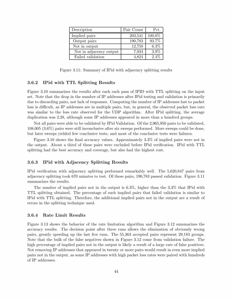
Description Pair Count Pct.

Implied pairs 203,541 100.0%

Output pairs 190,783 93.7%

Not in output 12,758 6.3%

Not in adjacency output 7,934 3.9%

Failed validation 4,824 2.4%

Figure 3.11: Summary of IPid with adjacency splitting results

3.6.2 IPid with TTL Splitting Results

Figure 3.10 summarizes the results after each each pass of IPID with TTL splitting on the inputset. Note that the drop in the number of IP addresses after IPid testing and validation is primarilydue to discarding pairs, not lack of responses. Computing the number of IP addresses lost to packetloss is difficult, as IP addresses are in multiple pairs, but, in general, the observed packet loss ratewas similar to the loss rate observed for the UDP algorithm. After IPid splitting, the averageduplication was 2.28, although some IP addresses appeared in more than a hundred groups.

Not all pairs were able to be validated by IPid Validation. Of the 2,965,950 pairs to be validated,108,005 (3.6%) pairs were still inconclusive after six sweeps performed. More sweeps could be done,but later sweeps yielded few conclusive tests, and most of the conclusive tests were failures.

Figure 3.10 shows the final accuracy values. Approximately 3.3% of implied pairs were not inthe output. About a third of these pairs were excluded before IPid verification. IPid with TTLsplitting had the best accuracy and coverage, but also had the highest cost.

3.6.3 IPid with Adjacency Splitting Results

IPid verification with adjacency splitting performed remarkably well. The 5,620,847 pairs fromadjacency splitting took 670 minutes to test. Of these pairs, 190,783 passed validation. Figure 3.11summarizes the results.

The number of implied pairs not in the output is 6.3%, higher than the 3.3% that IPid withTTL splitting obtained. The percentage of such implied pairs that failed validation is similar toIPid with TTL splitting. Therefore, the additional implied pairs not in the output are a result oferrors in the splitting technique used.

3.6.4 Rate Limit Results

Figure 3.13 shows the behavior of the rate limitation algorithm and Figure 3.12 summarizes theaccuracy results. The decision point after three runs allows the elimination of obviously wrongpairs, greatly speeding up the last five runs. The 55,363 accepted pairs represent 29,183 groups.Note that the bulk of the false negatives shown in Figure 3.12 come from validation failure. Thehigh percentage of implied pairs not in the output is likely a result of a large rate of false positives.Not removing IP addresses that appeared in twenty or more pairs would result in even more impliedpairs not in the output, as some IP addresses with high packet loss rates were paired with hundredsof IP addresses.

44

Description Pair Count Pct.

Implied pairs 81,637 100.0%

Output pairs 55,363 67.8%

Not in output 26,274 32.2%

Not in adjacency output 6,918 8.5%

Failed validation 19,356 23.7%

Figure 3.12: Summary of rate limitation results.

Description Pair Count

Input set 5,620,847

Pairs tested 2,908,033

After three runs

Rejected 2,607,481

Accepted 84,190

Inconclusive 216,362

After eight runs

Accepted 23,886

Rejected by 20 limit 14,272

Total accepted pairs 55,363

Figure 3.13: Summary of rate limitation behavior.

Rate limitation performed the poorest of the four algorithms. It had a high false negativerate, poor coverage, and medium cost. This is partially because less than 60% of hosts had ratelimitations, making coverage above 60% unlikely. Despite the fact that rate limitation is the poorestof the algorithms, it still found many pairs not found by any of the other three algorithms.

3.6.5 Splitting Comparison

There are three major goals of the splitting algorithms: reduce the set size, minimize the set overlap,and minimize the induced error. Figure 3.14 summarizes the two methods and the null method.Null splitting, provided for comparison, just outputs the input set. Adjacency splitting optimizesthe largest set, but covers less than half of the pairs. TTL splitting falls between the two, reducingthe largest set by a factor of ten while still keeping most of the pairs.

Pairs discarded by TTL splitting and adjacency splitting are much less likely to be valid pairsthan the pairs kept. As a result, the fraction of remaining pairs that are valid is much higher thanthe input set. The original set had 343,720 valid pairs, as measured by the union of the algorithms.That corresponds to one in 217,000 pairs being valid. For TTL splitting, that fraction went up toone valid pair in 12,600. For adjacency splitting, the fraction was even higher: one valid pair in27.4.

45

Method # Sets Total Size Pair Count Largest Set Coverage Pkts Sent

Null 1 386,157 74,558,421,246 386,157 100.0% 0

TTL 160 379,833 3,676,963,861 34,954 84.7% 466,756

Adjacency 5,620,847 11,241,694 5,620,847 2 59.7% 0

Figure 3.14: Summary of results for each splitting method. Pair count is the total number of pairsleft to test. Coverage is the percentage of pairs found by the combination of the methods thatappeared in at least one of the sets.

3.7 Conclusions

The IPid technique is clearly the most successful of the three techniques, finding the largest numberof sets and pairs, removing the most IP addresses, and having the smallest number of false positives.However, it required many more packets than any other technique. The UDP technique scales best,growing linearly with the input size. It is also the easiest to implement and has a low false positiverate (after private addresses and common invalid responses are removed). The rate limit techniquerequired the most number of packets and found the least number of sets. Moreover, it had thelargest estimated percentage of false positives.

Some combination of all three techniques are necessary for optimal coverage, as no technique hadbetter than 70% coverage. As each technique depends on behavior not specified by any standard,hosts are unlikely to be responsive to all three techniques. The coverage percentages show thatthere are a noticeable fraction of hosts responsive to only one of the techniques.

IP alias resolution is necessary to obtain a good measure of a topology using traceroutes. Notemploying any IP alias resolution algorithm could result in overstating the size of the network by40% or more. UDP techniques, while simple to use, only reduce the error from IP aliasing byapproximately a factor of two. If only one technique is used, IPid technique is clearly the one toselect, as it finds 87% of IP aliasing. Using all three techniques would get the best results, but isexpensive on large data sets. On medium and large networks, using IPid and UDP techniques willfind most IP aliasing at a reasonable cost. For smaller networks, such as a corporate network orthe network of just one ISP, combining the results of all three will result in the best topology whilenot being prohibitively expensive.

46

Chapter 4

Estimating the Reverse Routing Map

Good routing is central to the stable and efficient operation of the Internet. Understanding andimproving routing requires the ability to measure the current routing behavior. Routing can beviewed as a distributed algorithm in which each router makes local decisions that combine to definethe path between any two hosts on the Internet. Generally, routing is difficult to understandbecause its distributed nature makes it difficult to measure arbitrary routing decisions. Mostexisting routing-measurement systems are able to measure only one level of routing or examinepoint issues, such as BGP convergence.

The routing decisions of the Internet can be viewed as a matrix with a row for every routerand a column for every CIDR block. Each entry in this routing matrix contains one or more IPaddresses to which that router will forward a packet with that destination (the next hop). Routersmake decisions with near independence for each CIDR block. Even when the decisions are notcompletely independent, such as when adaptive routing is employed, the correlation between CIDRblocks is generally low.

One way to measure routing decisions is to use the techniques in Chapter 2 gather outboundpaths from a single measurement host to many destinations. Each path provides some of the entriesin the column corresponding to that destination. When the routing entries given by multiple pathsare combined, the set of routing decisions known is diverse. In terms of the routing matrix, thisgives scattered entries with little discernible pattern, making analysis difficult. Using multiplemeasurement hosts increases the number of entries known, but does not make the set any morecoherent. In contrast, each inbound path to a particular measurement host provides a set ofrouting entries all in one column. Combining many inbound paths gives information only withinthat column, which yields a simpler set to analyze.

Unfortunately, measuring inbound paths is much more difficult than measuring outbound paths.Several methods do exist, but they do not yield many paths. This chapter describes a method todetermine the routing decisions made by a large set of Internet routers for a particular destination.This set of decisions can be considered to be a directed graph with a node for each host. Themeasurement host is the “root” of the reverse routing map. An arc from node A to node B meansthat a packet routed through A towards the root will be forwarded to node B by node A. If thereis exactly one path from each node to the root, the directed graph is called a “tree”. This directedgraph is known as the “reverse routing map” for the measurement host. Given a reverse routingmap, paths from remote hosts to the root can be determined by finding a path within the map.

47

Given a set of inbound paths, the corresponding reverse routing map is the union of the paths.

This chapter presents a novel method to estimate the reverse routing map for a measurementhost using the TTL field. While the new method is not as accurate as previous techniques, itdiscovers approximately fifty times as many routing decisions as previous techniques. Combiningthe new method with existing techniques produces a good estimate of the decisions made by therouting algorithms running on the Internet. The reverse routing map from the new method iscompared against previous methods in terms of accuracy, precision, and coverage.

Section 4.1 explains known techniques to estimate the reverse routing map. Section 4.2 givesthe new method. Section 4.3 analyzes the output of the new method, both by itself and combinedwith previous techniques. Section 4.4 presents conclusions.

4.1 Previous Work

There are two previously-known ways to determine a set of paths towards a location: traceroutesfrom remote locations and loose source routing. Both of these techniques provide limited data,although the data they do provide is highly accurate.

4.1.1 Traceroute Servers

One way to get inbound traceroutes is to do traceroutes from remote locations. This requiressome access to the hosts in order to do the traceroutes. Gaining full access to a large number ofhosts with diverse connectivity is difficult and expensive. Fortunately, full access in not necessary.Because traceroutes from remote locations are also helpful in diagnosing problems, some peopleand organizations operate servers to perform such traceroutes as a public service. Such servers areknown as traceroute servers[51]. Traceroute servers can provide a variety of functions in additionto basic traceroutes, such as BGP table entries and ping, but only traceroutes are necessary forthe purposes of this chapter. Traceroute servers are accessible using HTTP[38], but the queryformat varies between servers. Thus, collecting a large set of traceroutes requires dealing withthese differences. Traceroute servers can be used to gather traceroutes from servers around theworld at little or no monetary expense and with minimal time investment.

The set of traceroutes gained from such servers is limited to the available traceroute servers.Unfortunately, many traceroutes are necessary to build a reverse routing map of any reasonablesize. Presuming each traceroute is twenty hops long, the first traceroute adds twenty nodes tothe reverse routing map. However, later traceroutes add fewer nodes to the reverse routing map,as some hops coincide with previous traceroutes. Presume that each new traceroute provides sixadditional nodes on average (this value is from results in Section 4.3.2). To build a reverse routingmap that covers 50,000 nodes, more than 8,000 traceroutes are necessary. There are approximately700 servers listed on http://www.traceroute.org[51]. Even without removing stale links, brokenconfigurations, and those servers that do not provide traceroute functionality, this is well short ofeven the 8,000 under-estimate of the number of traceroutes necessary. The alternative of findingor placing 8,000 hosts around the world is not tractable by any but a handful of entities.

Remote traceroutes produce an accurate, if limited, reverse routing map. This is useful for tworeasons. Firstly, the more hosts that use a link to access the root of the tree, the more likely it isthat at least one of the remote traceroutes traverses that link. Thus, the parts of the Internet used

48

by many hosts to access the root of the reverse routing map are likely to be contained within thereverse routing map. Secondly, remote traceroutes provide a baseline against which less-accuratetechniques can be compared.

4.1.2 Loose Source Routing

Loose source routing (LSRR)[76] is an IP option that allows a host to specify way-points throughwhich a packet should travel before reaching its final destination. LSRR provides an alternativeway to collect remote traceroutes. Consider an IP packet sent by a measurement host to itself,but loose source routed through a remote host. The path of such a packet will first travel towardsthe remote host. After reaching the remote host, the rest of the path will be the inbound pathfrom the remote host. By sending a series of such packets with low TTLs in a similar manner totraceroute[46], the combination of the outbound and inbound path can be measured. Removingthe outbound path yields the inbound path from the remote host specified as the way-point.

The problem with using LSRR is that it is not widely available. LSRR can be used for nefariouspurposes. Specifically, LSRR can be used to circumvent improperly configured firewalls and othersecurity structures. This means that LSRR is often disabled within routers. As long as this isnot universal, it does not, by itself, cause major problems, as LSRR is designed to only requirecooperation of the way-points. In this case, only the single remote host though which the packetis routed would have to support LSRR. Each router that supported it would effectively act as aremote traceroute server, and as few as 8,000 such traceroutes may be needed, using the estimatefrom above. However, some ISPs drop any IP packet that contains an LSRR option. This meansthat any packet traversing some major ISPs, such as UUNet, cannot include the LSRR option. Asa result, LSRR is unable to produce any paths that traverse such ISPs, which greatly limits thecoverage. As the trend on the Internet today is to increasingly block LSRR, the effectiveness ofthis technique is expected to continue to decrease. Because LSRR is of limited use and expectedto become even more limited in the future, it is not utilized herein.

4.2 TTL Method

The basic idea of the new method is to apply the investigation methods of Sherlock Holmes: “whenyou have eliminated the impossible, whatever remains, however improbable, must be the truth”.Given the complete network topology, the options (the possibilities) a particular host has for thenext hop towards a destination are the adjacent hosts within that topology. The question is howto eliminate the impossible.

The IP header includes an eight-bit field called the time-to-live (TTL) value[76]. The TTL isdecremented by one for each router through which a packet travels. If the initial and final valuesof the TTL are known, the difference between those two values is the length of the path from thehost sending the packet to the host receiving it. For two hosts A and B which are adjacent inthe topology, a directed arc from host A to host B can be in the reverse routing map only if thelength of the path from host A to the measurement host is one more than the length of the pathfrom host B to the measurement host. Otherwise, it is impossible for the arc to be in the reverserouting map. Eliminating the impossible arcs leaves the true arcs and perhaps a few false ones.However, this elimination is possible only if the initial and final TTL values are known for packetsfrom nodes in the topology to the root of the reverse routing map.

49

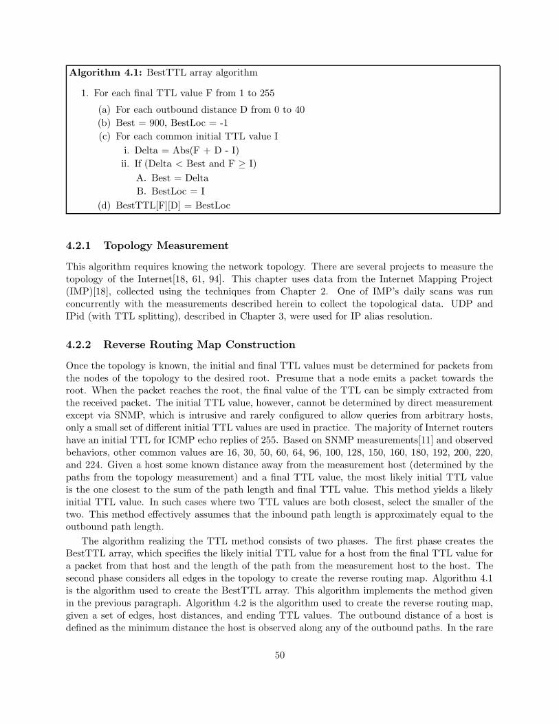
Algorithm 4.1: BestTTL array algorithm

1. For each final TTL value F from 1 to 255

(a) For each outbound distance D from 0 to 40

(b) Best = 900, BestLoc = -1

(c) For each common initial TTL value I

i. Delta = Abs(F + D - I)

ii. If (Delta < Best and F ≥ I)

A. Best = Delta

B. BestLoc = I

(d) BestTTL[F][D] = BestLoc

4.2.1 Topology Measurement

This algorithm requires knowing the network topology. There are several projects to measure thetopology of the Internet[18, 61, 94]. This chapter uses data from the Internet Mapping Project(IMP)[18], collected using the techniques from Chapter 2. One of IMP’s daily scans was runconcurrently with the measurements described herein to collect the topological data. UDP andIPid (with TTL splitting), described in Chapter 3, were used for IP alias resolution.

4.2.2 Reverse Routing Map Construction

Once the topology is known, the initial and final TTL values must be determined for packets fromthe nodes of the topology to the desired root. Presume that a node emits a packet towards theroot. When the packet reaches the root, the final value of the TTL can be simply extracted fromthe received packet. The initial TTL value, however, cannot be determined by direct measurementexcept via SNMP, which is intrusive and rarely configured to allow queries from arbitrary hosts,only a small set of different initial TTL values are used in practice. The majority of Internet routershave an initial TTL for ICMP echo replies of 255. Based on SNMP measurements[11] and observedbehaviors, other common values are 16, 30, 50, 60, 64, 96, 100, 128, 150, 160, 180, 192, 200, 220,and 224. Given a host some known distance away from the measurement host (determined by thepaths from the topology measurement) and a final TTL value, the most likely initial TTL valueis the one closest to the sum of the path length and final TTL value. This method yields a likelyinitial TTL value. In such cases where two TTL values are both closest, select the smaller of thetwo. This method effectively assumes that the inbound path length is approximately equal to theoutbound path length.

The algorithm realizing the TTL method consists of two phases. The first phase creates theBestTTL array, which specifies the likely initial TTL value for a host from the final TTL value fora packet from that host and the length of the path from the measurement host to the host. Thesecond phase considers all edges in the topology to create the reverse routing map. Algorithm 4.1is the algorithm used to create the BestTTL array. This algorithm implements the method givenin the previous paragraph. Algorithm 4.2 is the algorithm used to create the reverse routing map,given a set of edges, host distances, and ending TTL values. The outbound distance of a host isdefined as the minimum distance the host is observed along any of the outbound paths. In the rare

50

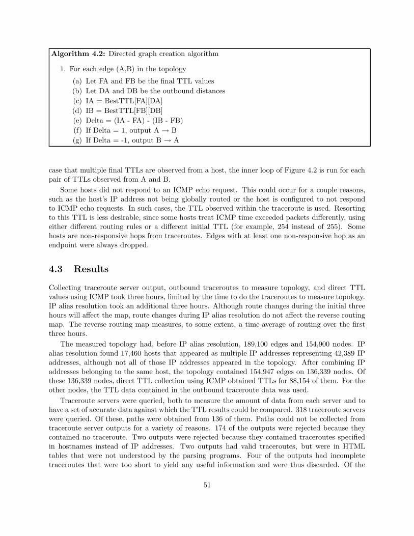
Algorithm 4.2: Directed graph creation algorithm

1. For each edge (A,B) in the topology

(a) Let FA and FB be the final TTL values

(b) Let DA and DB be the outbound distances

(c) IA = BestTTL[FA][DA]

(d) IB = BestTTL[FB][DB]

(e) Delta = (IA - FA) - (IB - FB)

(f) If Delta = 1, output A → B

(g) If Delta = -1, output B → A

case that multiple final TTLs are observed from a host, the inner loop of Figure 4.2 is run for eachpair of TTLs observed from A and B.

Some hosts did not respond to an ICMP echo request. This could occur for a couple reasons,such as the host’s IP address not being globally routed or the host is configured to not respondto ICMP echo requests. In such cases, the TTL observed within the traceroute is used. Resortingto this TTL is less desirable, since some hosts treat ICMP time exceeded packets differently, usingeither different routing rules or a different initial TTL (for example, 254 instead of 255). Somehosts are non-responsive hops from traceroutes. Edges with at least one non-responsive hop as anendpoint were always dropped.

4.3 Results

Collecting traceroute server output, outbound traceroutes to measure topology, and direct TTLvalues using ICMP took three hours, limited by the time to do the traceroutes to measure topology.IP alias resolution took an additional three hours. Although route changes during the initial threehours will affect the map, route changes during IP alias resolution do not affect the reverse routingmap. The reverse routing map measures, to some extent, a time-average of routing over the firstthree hours.

The measured topology had, before IP alias resolution, 189,100 edges and 154,900 nodes. IPalias resolution found 17,460 hosts that appeared as multiple IP addresses representing 42,389 IPaddresses, although not all of those IP addresses appeared in the topology. After combining IPaddresses belonging to the same host, the topology contained 154,947 edges on 136,339 nodes. Ofthese 136,339 nodes, direct TTL collection using ICMP obtained TTLs for 88,154 of them. For theother nodes, the TTL data contained in the outbound traceroute data was used.

Traceroute servers were queried, both to measure the amount of data from each server and tohave a set of accurate data against which the TTL results could be compared. 318 traceroute serverswere queried. Of these, paths were obtained from 136 of them. Paths could not be collected fromtraceroute server outputs for a variety of reasons. 174 of the outputs were rejected because theycontained no traceroute. Two outputs were rejected because they contained traceroutes specifiedin hostnames instead of IP addresses. Two outputs had valid traceroutes, but were in HTMLtables that were not understood by the parsing programs. Four of the outputs had incompletetraceroutes that were too short to yield any useful information and were thus discarded. Of the

51

traceroute servers that failed to return a traceroute, some failed because the HTTP request forthe traceroute was not in the form the traceroute server wanted. 65 of the traceroute serversfrom which traceroutes were not obtained requested a form to be submitted using POST. Thesetraceroute servers may have yielded paths if POST was used instead of GET. 23 of the tracerouteservers rejected their query because no referrer was given (they rejected it with a message statingthat no shortcuts are allowed). With further work, more traceroute server data could have beencollected. However, even twice as much additional data would not have changed the qualitativeresults.

Three different reverse routing maps were created: one derived purely from the tracerouteservers, one derived purely from the TTL method, and one derived from both pieces of data. Thesewill be compared against the real tree in three ways:

1. accuracy of the arcs excluded,

2. coverage of the map, and

3. how well the reverse routing map resembles a tree.

The accuracy of the arcs excluded is relevant for reverse routing maps derived from the TTLmethod. The TTL method discards arcs that it concludes are not in the reverse routing map. Howoften does it improperly discard an arc that should be in the reverse routing map? This will beevaluated by comparing the arcs from the traceroute servers, which are in the true reverse routingmap, against the results from the TTL method.

The coverage of a reverse routing map is the fraction of the Internet for which it providescomplete paths to the root. This can be measured both in terms of the nodes of the topology andaccess routers for edge networks. One of the stated reasons for using the TTL method was thetraceroute server data had poor coverage. How much has the coverage increased by augmentingthe traceroute server method with the TTL method?

Coverage only measures one part of precision; the other side of precision is how many extra arcsthe reverse routing map contains. The reverse routing map should be nearly a tree, but imprecisioncauses the reverse routing map to contain extra arcs. By comparing some properties of a tree withthe properties of the reverse routing map, this resemblance can be evaluated. The first propertyconsidered is that each node in a tree that is not the root has only one out-bound arc. The secondproperty considered is that there is only one path from each node to the root. For each node exceptthe root, its out-degree and the number of paths from that node to the root should be one. Howmuch do the true distributions differ from this?

4.3.1 Accuracy

Traceroute is generally considered an accurate method to determine the series of IP addresses alonga path. Thus, the traceroute server data should be accurate inbound paths from the server to theroot. The accuracy of the TTL method, therefore, can, and will, be measured by comparing itsoutput with the traceroute server data.

The traceroute servers yielded 136 paths representing a total of 833 arcs. The input topologycontained only 396 of these arcs. Of these, 19 (4.8%) were dropped by the TTL method. Thus,the TTL method is approximately 95% accurate in maintaining correct arcs. In contrast, only

52

Far node Near node Arc count

Within topology Within topology 64

Within topology Without topology 82

Without topology Within topology 131

Without topology Without topology 160

Table 4.1: Distribution of arcs in the traceroute reverse routing map but missing in the topology,separated by whether or not the endpoints of the arcs are in the topology.

35.5% of all arcs in the input topology were maintained. The bulk of the inaccuracy results frominaccuracies within the measured topology: 437 of the arcs from the traceroute server data (52.5%)were missing from the measured topology. Because the topology is considered an input to the TTLmethod, arcs missing in the input that should have been in the output are not counted against theTTL method. Such a large fraction of arcs missing from the input topology is, at first, alarming.However, these numbers overstate the incompleteness of the topology.

One explanation is that the topology used was based on traceroutes from a single source. Theobservant reader may wonder why only 48% of the arcs were in the topology when Barford, et al.[3]observed that 60% of the arcs are found using traceroutes from a single source. Clearly, there areother effects contributing to missing arcs besides the fact that only one source was used. Since thetraceroute server could be any host on the Internet, arcs missing from the topology could be theresult of firewalls, the outbound paths not containing the arcs, or simply not deeply exploring edgenetworks (i.e., not tracerouting to every possible IP address). The second case is what Barford, etal. attempted to measure.

To distinguish between output paths not containing the arcs and insufficient exploration, con-sidered whether the endpoints of the missing arcs are within the topology. If the arc is missing asa result of not using multiple sources, then the far endpoint should be in the topology. Insufficientexploration will result in arcs whose far end-point of the arc is not within the topology. Table 4.1gives counts of missing arcs with respect to whether or not their endpoints are within or withoutthe topology. Based on Table 4.1, 291 of the missing arcs were beyond the scope of the topologyand 146 were the result of missing edges in the topology. Thus, as a result of using a single-sourcetopology, about 17% of the correct arcs were not in the topology. 35% of the correct edges werenot in the topology because they were either beyond a firewall or they were in an unexplored edgenetwork.

4.3.2 Coverage

Coverage is the completeness of the information provided. In this case, coverage is the number ofIP addresses for which there is a complete path from that IP address to the root in the reverserouting map. This somewhat understates the true amount of information contained in the reverserouting map, as it ignores partial paths that do not connect to the root. This definition of coverageis designed to measure the reverse routing map’s ability to provide inbound paths.

Coverage will be measured by analyzing the reverse routing map that results from taking boththe traceroute server data and the output of the TTL method. Coverage, unlike accuracy, does

53

not require a source of accurate data to compare against. Thus, there is no need to withhold thetraceroute server data.

Coverage of nodes is straight-forward to calculate. Of the 136,625 nodes in the topology orthe traceroute server output, 52,024 nodes have paths to the root in the output reverse routingmap. Thus, the node coverage is 38.2%. If only the traceroute server data is used, 807 nodesin the reverse routing map have paths back to the root, an average of 5.93 per traceroute serverused (hence the figure of six hops per traceroute used in Section 4.1.1). The node coverage of thetraceroute server data is 0.6%.

Coverage of nodes is arguably a poor measure of coverage of the Internet, as nodes are generallyrouters which neither generate nor receive much traffic. An alternative coverage is the fraction ofrouted IP addresses for which a path exists within the reverse routing map from that network tothe root. The difficulty is defining what network an IP address is on. One way to do this is toutilize the traceroutes from which the topology is derived. Each path in the topology measurementis based on targeting a random node in a CIDR block. The last hop on each path represents thelikely access point for that CIDR block, at least from the viewpoint of the measurement host. Thisprovides a (mostly accurate) way to assign CIDR blocks to nodes in the topology. A local BGPfeed includes announcements representing 1,275 million IP addresses. The nodes that have pathsto the root in the combined reverse routing map represent 570 million IP addresses, yielding CIDRcoverage of 48%. Using only the traceroute data, 14.5 million IP addresses are covered, a CIDRcoverage of 0.8%. This analysis weights CIDR blocks by the number of IP addresses which theycontain.

Although neither the node nor CIDR coverage of the combined reverse routing map exceed 50%,the TTL method has greatly expanded on the output from traceroute servers. By augmenting thetraceroute server data with the TTL method, the coverage has increased by a factor of 64 in termsof the number of nodes and 39 in terms of the number of IP addresses represented.

4.3.3 Tree Resemblance

As defined, perfect coverage and accuracy could be obtained by discarding no edges. Of course,the resulting reverse routing map would be useless. The missing requirement is that the reverserouting map should resemble a tree. Although the actual reverse routing map is not a true tree dueto vagaries of Internet routing, it is close to one. Thus, the measured reverse routing map shouldbe nearly a tree as well. As it is difficult to quantify how closely a graph resembles a tree, threedifferent methods will be employed: degree distribution, path count, and path spread, the last tobe defined shortly.

Perhaps the most obvious method to compare the reverse routing map to a tree is to examinethe distribution of the out-degrees of the nodes in the output reverse routing map. If the reverserouting map were a tree, the out-degree of all nodes but the root would be one. Figure 4.2 gives thedistribution of out-degrees and, indeed, shows that 93.5% of the nodes (48,581) have an out-degreeof one. A few of the nodes do have large out-degrees: the top 0.1% of the nodes have out-degreesfive or greater and three nodes have out-degrees above ten. However, for most nodes, the outputreverse routing map gives a single next hop.

An alternative measure of tree resemblance is the number of different paths in the output reverserouting map from each node to the root. In a tree, there is one path from each node to the root.Figure 4.3 shows that, for most nodes, the output reverse routing map has no more than two paths

54

0

2

4

6

8

10

12

14

16

0.93 0.94 0.95 0.96 0.97 0.98 0.99 1

Out

-Deg

ree

Fraction of Nodes

CDF of Out-Degree

Figure 4.2: Distribution of out-degree of nodes in the output reverse routing map of the full method.Note that the x-axis begins at 0.93

1

10

100

1000

0 0.2 0.4 0.6 0.8 1

Num

ber

of P

aths

Fraction of Nodes

CDF of Number of Paths to Root

Figure 4.3: Semi-log plot of distribution of number of paths from nodes in the output reverserouting map to its root.

to the root. 39.6% of the nodes have a single path to the root and 31.1% have only two. Less than1% of the nodes have more than 50 paths, although a few nodes have more than 400 paths.

Purely counting paths does not consider how different the paths truly are. To correct this, lookat the average number of different IP addresses each distance from a node, which will be referredto as the “path spread” of a node. The path spread measures how many different nodes the outputreverse routing map gives as possible hops along the path from a node to the root. In particular,the path spread of a particular node A is the number of nodes on paths from A to the root ofthe output reverse routing map divided by the minimum distance indicated by the output reverserouting map. For a pure tree, the path spread should be one for each node, indicating that thereis only one path from each node to the root.

Path spread gives a better notion of precision than simply counting paths. To see this, considerthe cases shown in Figure 4.4. In both the left and right graph, the number of paths from theright-most node to the root (on the left) is two. However, the two paths in the left graph differin all hops except the first and last. In such a case, the path spread is nearly two. In the right

55

Path count = 2 Path count = 2Path spread = 12

7= 1.71 Path spread = 8

7= 1.14

Figure 4.4: Difference between path spread and path count. Path counts and path spreads are forthe right-most node of the graph.

1

1.5

2

3

4

0 0.2 0.4 0.6 0.8 1

Pat

h S

prea

d

Fraction of Nodes

CDF of Path Spread

Figure 4.5: Distribution of path spread in output reverse routing map plotted on a semi-log plot.

case, the two paths are similar, differing in only one hop. In such a case, the path spread is nearlyone. Path spread correctly identifies the right case as better, while path count does not distinguishbetween the two.

Figure 4.5 shows the distribution of path spread. 39.6% of the nodes have a path spread ofexactly one, corresponding to the 39.6% of the nodes that have exactly one path to the root. Beyondthat, path spread makes it clear that although many nodes have multiple paths to the root, mostof those paths are similar. A majority of the nodes (89.6%) have path spreads below 1.5, meaningthat at least half of the hops along the reverse path are known (only one possible host for thathop).

4.4 Conclusions

Previous techniques to determine the reverse routing map have poor coverage. Both LSRR andtraceroute servers depend on gathering remote traceroutes from many different locations. To cover50,000 nodes would require at least 8,000 remote traceroutes and still not be full coverage of theentire Internet. LSRR is blocked by many ISPs and blocking LSRR is increasing in popularity.There are around 700 traceroute servers, a factor of eleven below the minimum required amount.Thus, obtaining a reverse routing map with good coverage requires new techniques.

56

The TTL method detailed herein provides much better coverage than previous techniques.When combined with traceroute server data, the resulting reverse routing map covers 38.2% of thenodes, compared to 0.6% coverage using only the traceroute server data. This technique is not asaccurate as previous techniques, but maintains 95% of the correct arcs while dropping 64.5% of allarcs.

Besides removing some arcs that it should not, the TTL method includes some arcs in thereverse routing map that should not be included. This manifests itself as multiple paths fromnodes to the root. Although there are often multiple paths from nodes back to the root, they donot differ greatly. For 89.6% of the nodes, path spread shows that the various reverse paths offeronly a single possibility for at least half of the hops.

Improving the input topology would improve the results. 28% of the arcs included in the trace-route server were not in the input topology. Using multiple sources for the topology measurementor scanning over multiple days would improve the topology, although that would sightly complicateTTL collection, as the majority of TTLs collected by topology measurements would either be fora different measurement host or old data.

One drawback of the TTL method is that it requires access to the root of the reverse routingmap. Loose source routing has no such restriction. As some traceroute servers will only tracerouteto the host requesting the web page, fewer traceroute servers would be useful if no access to theroot was available. This would cause decreased coverage, but the traceroute server technique couldstill be used.

This chapter presented the first technique to estimate the reverse routing map for a measurementpoint that covers a significant portion of the Internet. The limited output from previous techniquescan be used to augment the estimation provided by this new technique, producing a combinedreverse routing map. The combined reverse routing map is a good estimate of the routing decisionstowards a particular destination for a considerable fraction of the Internet.

57

58

Chapter 5

Tracing Anonymous Packets1

One of the major problems on the Internet is denial of service (DoS) attacks against hosts andnetworks. As compared to other attacks, these are attempts to limit access to a host or serviceinstead of subverting the service itself. DoS attacks are simple to design and implement, and thereis a plethora of readily available source code which will perform the task. The idea behind mostDoS attack is to send a stream of packets towards a victim such that the victim is unable to serveits clients because it is too busy serving the ‘clients’ that the attacker is emulating.

There are two basic targets of DoS attacks: hosts and the network. SYN attacks[12] are anexample of an attack against a host. In these attacks, a series of TCP SYN packets are sentto a host, which causes the host to create a lot of half-open TCP connections. When a realclient wishes to connect, the host cannot find an open slot in its table for the client, resultingin the connection being denied. The basic problem with this attack is that clients and attackersare almost indistinguishable, except that clients respond to the TCP SYN/ACK packets the hostreturns, while attackers do not. This particular kind of attack has a known defense[12], althoughother host attacks may be more difficult to defend against.

The second target, the network, is a much more difficult problem. Here, the target is to overloada company’s connection to its ISP with traffic. In particular, the attacker causes a large stream ofdata to flow towards the company. This results in overloading in the pipeline from a company’s ISPto the company, causing packet loss. Since routers cannot distinguish between attacking packetsand valid clients’ packets, they drop them with equal probability. If the attacker can send packetsquickly enough, the drop rate can rise enough that an insufficient number of clients’ packets getthrough. This results in clients not being able to get reasonable service from any host through theloaded link. A common form of this type of attack is the smurf attack[13]. Distributed denial ofservice (DDoS)[14] attacks are generally also of this flavor.

The major advantage of DoS attacks, from the attacker’s perspective, is that it is extremelydifficult to determine the actual source of the attack. Since the attacker can put almost any packeton the local wire, the attacker creates packets whose source IP address is invalid and random.When the victim receives these packets, they are unable to determine the source. The currenttechnique for tracing a packet stream back to the source requires cooperation of all the intervening

1This chapter represents work with William Cheswick, originally published as “Tracing Anonymous Packets toTheir Approximate Source” at 2000 USENIX Lisa[8].

59

ISPs. This is something that is difficult to obtain, since the victim is rarely a customer of all of theISPs between it and the attacker. This technique will be discussed in more detail later.

This chapter presents a method to trace a steady stream of anonymous Internet packets backtowards their source. The method does not rely on knowledge or cooperation from interveningISPs along the path. In addition, tracing an attacking stream requires only a few minutes oncethe system is set up. The results presented herein represent work started eight years ago andpublished five years ago. Although much later work has been done based on this work, the techniqueitself may no longer work. Its effectiveness is somewhat moot anyway, as most attackers nowuse distributed denial of service attacks, where the main technique described is not useful. Thealternative techniques discussed, however, remain useful.

The basic technique is given in Section 5.1. Section 5.2 lists the assumptions made. Section 5.3discusses various network loading procedures. The results are detailed in section 5.4. Alternativesolutions are listed in section 5.5. The antisocial aspects of this approach are discussed in section5.6. Section 5.7 covers some of the work since the original publication of this work. Section 5.8presents the conclusions.

5.1 Basic Technique

The technique begins by creating a map of the routes from the victim to every network, usingany known mapping technology[17, 42, 61]. Then, starting with the closest router, the techniqueapplies a brief burst of load to each link attached to it using the UDP chargen service[77]. If theloaded link is a component of the path of the attacking stream, the induced load will perturb theattacking stream. Thus, if the stream is altered when a link is loaded, this link is probably alongthe path from the source host of the attack to the victim host. If the strength of the stream isunperturbed by the load, it is unlikely that the stream of attacking packets is utilizing that link,making it unnecessary to examine the networks “behind” that link.

The technique continues working back through the network router by router, pruning branchesthat do not perturb the attack, as the technique tries to narrow the attack source to one network, atwhich point more standard trace-back techniques can be employed by contacting the entity whichcontrols that network.

Executing a trace effectively does require significant preparation in the way of data collection.The technique needs data collected from the network, as well as traceroutes from the victim toall possible networks. Due to asymmetric routes, naively, directional data must be collected andmaintained by reverse traceroute servers or the techniques of Chapter 4 in order to have betterdata. One way to avoid this is to collect outbound paths and assume that the incoming pathsare approximately the reverse of those paths. While this is not completely accurate, collecting thepaths to all networks determines what links could be used on a path from a given network to thevictim’s network. Thus, this assumption does not cause as much inaccuracy as might otherwiseoccur.

Because the technique must be able to induce isolated load on specific network segments thatare not in its purview, it is necessary to identify sources “willing to” (read: will) perform that task.It is known that ISPs quite regularly turn off the services that this technique exploits to inducethese loads. Thus, the technique must identify cooperative hosts at the right places in the networkmap in order to produce the required load.

60

This element of the technique is worrisome, since it constitutes a brief denial-of-service attackon that network link. Hackers already employ bulk versions of this approach for denial-of-serviceattacks. This technique, on the other hand, carefully limits load to segments only long enough torule them out as a possible component of the suspected path. The difference is analogous to thatbetween a sword and a scalpel. In any case, the antisocial aspect of this technique is recognized, andthe tool should be used rarely and only in appropriate situations. Possible customers include lawenforcement, the military, ISPs, and perhaps companies policing their own private intranetworks.

Before attacks or victims are even known, a trusted host must develop and maintain a currentdatabase of networks and load generators. The current version of the tool executes the trace fromthe victim (targeted) network, but a sufficient complete map of the Internet might allow a neutralthird party to run the detecting utility, which would allow flexibility in where to spread some ofthe bandwidth costs of the tool.

In either case, the tracing host emits packets that stimulate traffic flow through a desired routeror link. A visual display of various statistics of the incoming packets on the victim’s network helpsdetermine if that link is used by the packets.

The trace-back is done manually. Though there are algorithms that might automate this process,requiring that a human manually apply the load to the link reduces the cost of programming errors.The programs are designed to supply the operator with information about the amount of load sheis inflicting on networks, and she can chose to stop using networks that have already be heavilyused.

If the induced load is sufficient to induce drops of incoming packets, it quickly and dramaticallyaffects the attacking flow. The discomfort to ISPs and end users is brief enough that it is likelyto escape notice. If the load does not induce loss, it may be necessary to run the load generatorslonger and seek more subtle effects on the workload. This technique appears to work better whenthe network is already heavily loaded, though one can imagine more subtle statistical effects thatmay be detectable when the Internet is relatively quiet. Attempts, however, to discover such effectshave met with little success.

5.2 Assumptions

The presented traceback technique relies on several assumptions, but experience indicated they wereoften valid and that the technique would work. These assumptions, particularly the assumptionsabout hacking behavior, are probably no longer true.

5.2.1 Assumptions About the Internet

Because of the way the search is done, the technique requires that most routes over the Internetare symmetric. Asymmetric routes confuse mapping, trace-back, and loading. However, the pro-liferation of reverse traceroute servers, which has proven quite useful for network diagnosis anddebugging, might also facilitate construction of at least a partial directional map of routes. Tech-niques from Chapter 4 to build an approximate reverse map would also make this assumptionunnecessary.

It is also assumed that enough load can be applied to a particular Internet link to affect perfor-mance statistics, in particular loss, of the stream of attacking packets. Enough packet generators

61

beyond the tested link must be available to load it, which can be challenging across infrastructurewith fast links and slower downstream networks. The techniques for doing this will be discussedbelow, as well as experiments on how true this is.

5.2.2 Hacking Behavior

One of the largest assumptios is that the attack is from a single host. In addition, the attack mustbe at a consistent rate and continue for a reasonably long time. Denial-of-service attacks are morevexing if they are ongoing, and some attacks have lasted for weeks. The technique requires timeto move equipment and programs into place, map routes, and perform the actual trace-back. Thisassumption was often true at the time of the original work. Today, this assumption is no longervalid, as most DoS attacks are distributed.

Because bizarre behavior can occur during the trace-back, the technique must make as effectiveuse as possible of the clues gathered. For example, the operator might notice an attacking stream’sstatistics are perturbed by 1/3 rather than dropping off entirely. Such behavior would be consistentwith two or three concurrent attacks from separate hosts (it also possible that the attacking streamis being load-balanced across three different links). Unfortunately, only one packet stream can betraced at a time, if that. Thus, being able to distinguish among the streams would be essential tobe able to perform the trace. This may be possible using other clues in the packets. For example,the operator might be able to distinguish between a few attacking streams using the arriving TTLvalue, assuming packets within each stream are launched with the same TTL value, and with eachstream from different hop distances away. In practice, DDoS attacks are believed to come frommany hosts. It is likely to be difficult, if not impossible, to distinguish many attacking streams.

It is assumed that the attacker does not know that their packets may be traced. An effectivehacker attacks from co-opted hosts and never returns to the attacking host. She hides her trailthrough a thread of login sessions across many hosts and networks before attacking the target.Of course, TCP-based attacks require bidirectional packet flow between the attacker and victim,making this technique unnecessary. The denial-of-service attack targetted with this tool is a one-way packet flow, which does not rely on interactive login sessions.

In addition, it is assumed that there is something forensically interesting at the source of theattack. The effort of running the traceback tool may not be justified if the result is just disablingone attacking host or convincing one community of computers to enforce valid source addresses.The technique may be able to catch someone who was not cautious because he did not expecthis packets to be traced (the difficulty of the tracing task renders this a common assumption ofhackers).

Lastly, the attacker must not be familiar with the techniques listed here. These techniques canbe easily thwarted in several ways, including modifying the attacking program to vary the sourceof the attack, altering the frequency of the packets randomly, and attacking from many differentsources.

5.3 Network Load: No Gain, No Pain

Once the path from each network on the Internet to the victim has been determined, either bymeasuring forward paths using the techniques of Chapter 2 and assuming symmetry or using

62

reverse techniques described in Chapter 4, the trace-back is done by walking backwards throughthe resulting directed graph. The technique loads a link, hopefully causing enough packet loss tonoticeably decrease the rate of attacking packets. If a significant drop occurs, there is good reasonto believe that the tested link is on the path from the attacker to the victim. Otherwise, either thelink is not on the path or the load, or ‘pain’, applied to that link was insufficient to incur packetloss. Note that since most links are full duplex, the link must be loaded in the direction towardsthe victim.

This traceback requires making a high capacity link busy for a short period of time, usually asecond or two. It is difficult to generate a flow of packets from a single host or network that will dothis. It would have to come from a fast host on a fast, unloaded link. Ideally, the technique wouldutilize some leverage, some “gain,” on packets it emits. That is, if the technique sends out a flowof size x, the resulting load across link of interest should be of size kx, were k, the gain, is large.Since the rate that packets are sent is limited by several factors, such as the initiating network andthe initiating host, low gains mean that the resulting load will not be sufficient to alter the packetrate.

In the early days of ARPANET, mailing lists were full of discussions of situations of the desiredtype, talking about routing loops and exponential problems such as broadcast storms. Thesediscussions resulting in an Internet that has been carefully engineered to avoid allowing a singleemitted packet to cause a lot of resulting packets. This is certainly a good thing for the Internet,because if it was possible to get a huge gain, then hackers would be exploiting the design flaw. Infact, the smurf attack[13] exploits one flaw that was not fixed.

To produce the load, the technique sends a series of messages, such as ICMP echo request(ping) packets[75], from the victim’s network out to some distant networks whose return paths areexpected to include the link to be loaded. However, an ICMP echo request packet only gets onebyte in return for every byte sent, which is a gain of only 1. In addition, the return packets traversethe entire path back to the victim, which loads the entire set of links from the assistant networkto the victim, which obscures the data when trying to determine, say, the third link out. SendingICMP echo requests from a separate network dedicated to this service is also problematic, sincethe nature of Internet routing means that it is hard to assure that their return path traverses thelink being tested.

The technique solves the obfuscation problem by sending spoofed packets. When testing aparticular link, probe packets are sent to the router on the far end of the link, using as a returnaddress the router on the near end of the link. The near router indignantly discards the unsolicitedreplies (if using TCP, it actually may reset; for UDP, it may reply with a ICMP Port Unreachable).Thus, the return packets traverse only the link of interest.

5.3.1 More Gain

There are additional problems with using ICMP echo requests. Many routers make special effortsto put rate limits on handling of ICMP echo requests, since they are sometimes used in attacks.More importantly, a gain of 1 makes loading a backbone link difficult, if not impossible. Thus, adifferent service to supply the load must be found.

The most obvious choice of service to employ is the often-overlooked tiny service TCP charactergenerator (chargen)[77]. This service generates continuous data to anyone who connects to it,exactly what is desired. The rate of data flow is limited in general by the rate that the data is

63

acknowledged by the client host. At the cost of a few TCP ACKs from the victim, the techniquecan coax a steady stream of data out of a site supporting this service. Several of these streamsrouted over the target link will generate substantial load. In theory, TCP ACKs could be used topulse all the transmitters, providing a fine burst of load by ACK-ing several open chargen socketssimultaneously.

As TCP chargen was implemented as part of this technique, two major problems arose: theTCP processing on the local host slowed this chargen stream down more than desired, and, moreimportantly, the chargen stream must traverse the path all the way back to the sender, unless muchmore complex techniques, such as TCP sequence guessing, are used. This second problem can bemore easily circumvented by using UDP chargen instead of TCP, and spoofing the packets, butthis method provides little gain, usually around 102 bytes back for each sent packet of 40 bytes2, again of only 2.55. The chargen RFC specifies that the return packet should have between 0 and 512bytes of data[77] (not counting the 28 bytes for the IP and UDP headers[76, 74]). Some WindowsNT 4.0 hosts, however, violate this standard and return up to 6,000 bytes in response to a singlepacket, a gain of 150.

A spoofed ICMP echo request to a broadcast address can yield gain as well. By locatingnetworks ‘beyond’ the link to send broadcast ICMP echo requests to, the technique gets a gain ofone for each host on that network which responds. Unfortunately, many routers process broadcastICMP echo requests in such a way that only the router on the network returns a packet. Thisis, of course, fortunate for potential victims of broadcast ICMP echo request attacks, and is, infact, recommended for that reason[13]. However, for the purposes of this technique, it limits theusefulness of broadcast ICMP echo requests.

Such routers do let other broadcast traffic through, however, and experiments showed that gainsin excess of 200 can be obtained quite often using broadcast UDP chargen packets. Surprisingly,many networks within Lucent still respond to broadcast address 0 instead of 255. Therefore, bothhad to be checked to determine the correct one for each network. Figure 5.1 shows a distributionof networks and their gain for Lucent’s intranet. Note that the networks with a gain of less than 1have a gain of 0, which means that they did not respond to broadcast UDP chargen at all.

The goal of the load is to load one line or, maybe, one router. Loading the entire path backis certainly undesirable. This is prevented in two different ways: First, as mentioned above, thereturn address of the UDP chargen packets is spoofed to be the address of the router on the victim’sside of the link. Second, the technique utilizes multiple UDP chargen hosts. To test a link, thetechnique selects networks that reside behind the link, as seen from the victim. In particular, thetechnique selects networks that have hosts that respond to UDP chargen broadcast packets andwhose reverse paths are believed to traverse the link to be tested. This strategy focuses the loadon the link under examination; the load packets travel to the far router over mostly disjoint paths,affecting each other little. The returning packet paths then join at the far end of the link, traversethat link, and end. The load is limited by the lines the load must traverse, the speed of the networkswhere the load is being generated, and the ability of the measurement host to generate packets toemit the UDP chargen packets.

Experimentally, the average gain observed in Lucent is around 133.8, ignoring one networkthat has a gain of several tens of thousands (a factor a 25 above any other), due to oddities in

2Sent packets consist of a 20 byte IP header, a 8 byte UDP header, and 12 bytes of data that gives informationabout the source of the packets, since they are spoofed.

64

1

10

100

1000

0 100 200 300 400 500 600 700 800 900

Gai

n

Host

Figure 5.1: Distribution of gains seen using the broadcast address for Lucent’s intranet. Thenetwork that generated a gain 43,509 and is excluded from this graph.

A B

R4

R5

R6R7

R3

R2

R1

Victim

Attacker

attacking packets

chargen resp chargen resp

UDP chargen requests

Figure 5.2: Example of trace-back step. Packets are sent to A and B, spoofed from R2, in orderto initiate packet flows towards the victim. This causes increases congestion along the R3-R2 link,which, if sufficient, will induce packet loss.

65

Line Type Gain Required

10Mbps Ethernet 12.5

100Mbps Ethernet 125

1Gbps Ethernet 1250

T1 1.9

T3 56

OC-12 777

OC-48 3,110

OC-192 12,441

Table 5.3: Required gains to load a variety of line types, assuming 800 kbps of emitted packets andno packet loss.

its configuration (discussed below). A host can generate 2,500 40-byte packets per second withouta problem, a total of 800,000 bits per second. To flood a 10Mbps Ethernet only requires a gainof 12.5. Table 5.3 shows the necessary gains to load a variety of line types. In order to flood abackbone link, such as an OC-48 or OC-192, the gain must exceed 3,000, which is larger than all butone of the observed gains. However, when loading links, the link is already partially loaded by therest of the traffic that is traversing those links. Thus, the actual amount of traffic required to startpacket loss is less than the number in Table 5.3. Also, because this technique is no longer sensitiveto the location from which the load-inducing packets are sent, the rate of outbound packets couldbe increased greatly by using multiple computers that connect to the Internet over different links.

From the numbers of Table 5.3, it is clear that the hardest problem is usually tracing through thewide-area network. Besides requiring a large gain, testing links on the wide-area networks is difficultbecause, by the time the chargen packets get to the link under examination, congestion-induced lossthrough previous routers has diluted the stream. The technique overcomes this difficulty by usingseveral chargen generators whose paths do not coincide until the target link. This will be referredto as ‘focusing’ the load. Focusing can also alleviate the problem of testing lines that are nearer andfaster than lines behind them. However, backbone links are already loaded, especially during peaktimes. Thus, it may not require adding as much traffic to the link to noticeably increase packetloss.

Thus far, only techniques for loading a link have been considered; another possibility is to loadthe router. Diverting packet flow by sending a message directly to a router is quite difficult, asInternet backbone routers ignore various ICMP messages to redirect or stifle packet flow. Mostmethods to load a router have to tackle its system configuration to limit return data flow. Routerdesigns also typically have almost all forwarding handled by a simple host that delegates difficulttasks to a higher layer. Less legitimate options, such as hijacking BGP sessions or breaking intothe router itself, are too malicious to be seriously considered.

There are other possibilities for ways to slow routers, however. One option is to ping-flood therouter, i.e., send it ICMP echo requests as fast as possible. A similar alternative is to send therouter a flood of packets whose Time to Live (TTL) value expires at the desired hop along thepath, or to transmit a stream of UDP packets to high ports to stimulate responding UDP portunreachables. Since most routers appear to rate-limit UDP port unreachable messages, this ideawas abandoned before testing it extensively. Other methods do not seem to have a major effect.

66

Another idea is to attempt to upset the router’s routing table by spewing packets at the router.That is, find some sort of packet it responds regularly to (TTL exceeded, echo request) and sendit a bunch of packets with random return addresses. Coping with the packets may require enoughattention to unsettle the route table cache. In order to combat the incoming stream, it may beuseful to pick a handful of sources and cycle through them. This approach has not shown muchpromise when used within Lucent, perhaps because most Lucent routers use only a single defaultroute to avoid making forwarding cache state a resource issue.

5.4 Results

To test the technique, logins were obtained on various hosts throughout Lucent’s intranet. A non-privileged program named sendudp was written and run to generate a stream of packets back to anonexistent host on the same network as the tracing host. In most cases, the technique was able totrace the packets back to the “attacking” building. In many cases, the technique could trace backto the individual Ethernet segment.

Some links did not respond to an applied load. In some cases, it was necessary to go a hopbeyond the non-responding links (all the links that are connected to a host that are one hop awayfrom where the technique had traced back to) in order to find a link which, when loaded, affectedthe packet flow. Sometimes, it was possible to pick up enough of a signal from one of these nextlayer links that the trace-back could continue. It was a quite manual process, however, which couldbecome difficult when an untestable link had a large number of incident links.

With two exceptions, corporate users appeared to be ignorant of the tests. If the mapping issubtle, and the load applied for short periods, users are unlikely to notice the performance hit,or dismiss it as normal network variability. Early on, testing was confined to a few networks,and the network administrator received enough complaints to notice the activities several times.Subsequent tests appeared to go unnoticed, though in both cases there no attempt to hide theexperimental activities. On one network used to generate load, the broadcast UDP chargen packetinitiated a broadcast storm on their network. This network had a gain in the tens of thousands.Local users definitely noticed every time it was used, since it brought the network to a halt. Ofthe 2,000 networks in Lucent, only this one appeared to be unstable in this matter. The Internetlikely has an even lower rate of misbehaving networks.

5.5 Alternative Strategies

The proposed technique is hardly ideal. This section will discuss multiple alternative techniquesthat may be able to reduce the problems with denial of service attacks. Like the proposed technique,some techniques provide mechanisms in the network to trace anonymous packet streams. Othertechniques address the problem by reducing or eliminating the ability of hosts to produce anonymouspacket streams. This list is by no means complete, but it gives some of the more promising methods.

5.5.1 Filter Return Addresses at the Source

The most desirable way to solve the problem of anonymous packets is to enforce correct sourceaddresses at or near their source via a method called ingress filtering[37]. A company or university

67

should block outgoing packets that do not have appropriate return addresses. ISPs should havesimilar filters for each of their customers.

This solution is undoubtedly correct. Anonymous packets have no place on the Internet. How-ever, these filters have the unfortunate side effect of making life more complicated, and for largeusers behind slow routers, they can even degrade performance. For all users, these filters are anadditional administrative problem: one more thing to install, maintain, and get wrong. ManyInternet entities already have firewalls that enforce this policy, and several RFC’s recommend it asessential for any responsible participant in the global routing system. Most firewalls have the abil-ity and capacity to perform these checks. Source-based filtering may also upset mobile networkingmethodologies.

This solution also requires that most, if not all, Internet sites adopt this approach. ISPs wouldhave to agree to refuse to connect to other ISPs that do not enforce this strategy, a constraint thatmost ISPs do not impose at this time.

5.5.2 Filtering in Backbone Routers

Routers at the core of the Internet, those running BGP4 and exchanging full Internet routing tables,inherently enforce proper destination addresses on packets, since the routing system is built aroundforwarding the packet toward the value of this field. Theoretically, routers could perform a similarcheck on the source address, i.e., drop those with source addresses that are inconsistent with theirincoming interface.

Unfortunately, the verification is not nearly this simple, since a packet may come from morethan one possible incoming interface, requiring routers to maintain a huge amount of state. Notonly do routers not have spare memory resources to maintain this state, they do not have spareCPU resources to perform the verification. In the midst of sustained forwarding rates of millions ofpackets per second, often operating quite near, if not at, their maximum capacity, router designersmust optimize for speed. An additional lookup of the source information would require similaroptimization and subsequent re-engineering of many routers, an expensive and unlikely scenariounless ISPs are willing to pay for it.

One could imagine that legal fallout from a particularly damaging attack might force this sce-nario, and some routers may emerge that support such functionality service without re-engineering.In general, however, the industry has long resisted source-based policy routing, and there is littlereason to expect a fundamental change in this mind-set in the near future.

5.5.3 Tracing by Hand

The obvious ad hoc solution to finding a spoofing host is to trace packets back to their physicalsource manually. This method requires significant cooperation and attention from intervening ISPs,which has proven a problem in past incidents. They may not have the policy, inclination, time,expertise, or instrumentation to help out. Test equipment may not be available for some locationsor links within their network. For example, some Cisco routers have been known to crash if IPDEBUG is used under sufficiently heavy load.

Further, the traces may be needed off-hours: the Panix attack in 1996[108] started a littleafter five one Friday afternoon. It may be hard to find someone at any hour at the ISP who can

68

handle the technical details. Sometimes attacks are only solved because a victim happens to bewell-connected to admin-able friends at ISPs that are willing to help them out.

This cooperation is helpful, but selective, and slows the process down immensely. A quickermethod would be extremely useful.

5.5.4 Shutting Down a Router

One could imagine sending a message to a router requesting that it drop all packets for a particulardestination for a about a second. This interruption would be long enough to detect a break inincoming packets, without noticeably affecting service. Implementing this feature would providean obvious denial-of-service attack of its own. The router could require that requests be stronglyauthenticated, but there is no infrastructure present for such validation in the current Internet.In self-defense, a router would have to do similar rate-limiting as it does with UDP responses,rendering the feature useless for a significant attack.

Given the ease with which an attacker can hide her attack, it probably is not worth deployingsuch a service. Without global support, an attacker will simply launch the attack from a placewithout this feature. This feature would be difficult to deploy and provide only limited usefulness.It is unlikely a large fraction of ISPs would be interested in deploying such a service.

5.5.5 Marking Packets with IP Addresses

Another alternative that has been suggested is to place the IP address of all the routers that apacket goes through during its flight across the Internet. This has two obvious disadvantages: itrequires CPU time of the routers and it increases the size of packets, especially in the case ofrouting loops. Both of these could be reduced by having it mark only every 1 in N packets througha given interface. If N is small enough, a long enough attack would give a complete list of routersalong the path, if not their actual order. If N is chosen large enough, the additional router timeand packet size increase would be negligible. In practice, randomly varying N may avoid possibleproblems with routers synchronizing. If N is too small, than the attacker can insert packets intothe network that can ‘fool’ the system into misdiagnosing the path. In practice, keeping only oneaddress in a packet at a time may be desirable to simplify the header.

5.6 Ethics

The proposed methods to trace-back anonymous packets resemble techniques used by hackers. Thisresemblance raises several ethical questions which must be addressed.

1. Does the tracing attempt cause more damage than the actual packets? If the answer is yes,then, obviously, this technique should not be pursued. It is not possible to provide a universalanswer to this question; it really depends on the situation. If the anonymous packet streamhas shut down the daytime service on a web server, it is perhaps not harming the operatorenough to take serious action. If the attackers are crashing the victim’s network and denyingcustomers access to the primary service of the victim, then perhaps stopping the attack isworth the cost of congesting a few network links for a few seconds (it almost certainly seems

69

worth it to the victim). This is a judgment call that must be made by any potential user ofthis method.

2. Does leaving a service (such as UDP chargen) enabled on a host implicitly mean the ownerhas given permission to use it? The technique does not attempt to gain access to privateinformation or crash individual hosts, but it does leverage accessible services from privatehosts. However, these hosts have left the UDP chargen enabled (or whatever service isemployed).

The easy answer is yes, but it harbors dangerously close to the common hacker defensethat leaving a service with possible security holes running indemnifies those who intention-ally exploit it. On the other hand, the technique does not really exploit a security flaw inimplementations. Indeed, the technique follows the intended protocol specification exactly.Nonetheless, the essence of the technique is the imposition of a denial-of-service of the at-tacker’s own denial-of-service attack against the victim.

After much consideration, the appropriate answer to this question appears to come down tomotivation. While a hacker is generally trying to harm the host, gain access to private information,or journey on an ego trip, the technique leverages the host for a secondary purpose that is helpfulto the Internet community.

This argument is almost assuredly insufficient to convince some organizations that reside onthe Internet that it is reasonable to use the presented trace-back technique.

5.7 Later Work

Since the original publication of this work, there have been many papers published in this area.Although there is little hope of including all the research, this section outlines the general lines ofresearch.

Much of the later work focused on probabilistic marking schemes as described in Section 5.5.5.Savage, Wetherall, Karlin, and Anderson[87] were the first to propose a specific method to mark thepackets and reconstruct the reverse path. Using 16 bits of IP header space, they designed a schemeto reconstruct a 30-hop path in 4,500 packets with 95% probability. Their scheme placed a partialmark into the packet with probability 0.04. These marks were then collected and correlated by hopand then combined to produce a coherent path. Their approach performed poorly for distributedattacks. Doeppner, Klein, and Koyfman[33] proposed a similar scheme based on adding IP optionsto the packet. Song and Perrig[93] refined the technique to reduce the number of false positivesthat occur in distributed attacks. Song and Perrig exploited knowledge of the network topology.They developed an approach designed to scale to a few thousand attackers. Dean, Franklin, andStubblefield[26] used algebraic techniques to achieve similar results. Their algorithm uses 25 bitsof the header, more than Sing and Perrig, but did not require knowledge of the topology.

Some theoretic results have followed. Lee and Park[71] analyzed how may alternative paths anattacker can spoof under probabilistic packet marking. Adler[1] analyzed the general problem of anetwork trying to communicate information (in this case, the attacker’s location(s)) statelessly.

Alternative approaches have also been proposed. In 2000, Bellovin proposed in an expiredIETF draft sending an “ICMP traceback” message instead of marking the packet. Ioannidis and

70

Bellovin[60] proposed distributed filtering. The idea behind their approach is that attack trafficis concentrated through a few routers while legitimate traffic is more evenly spread. By limitingthe amount of all traffic flowing through upstream routers to the victim, routers that forward onlylegitimate traffic see little traffic and will therefore forward all of it. Routers that see attack trafficsee a lot of traffic and will therefore filter both legitimate and attack traffic. The net result is thatmuch of the attack traffic will be filtered before it gets to the victim. The further upstream thisfiltering can be pushed, the less attack traffic the victim will see.

These two approaches have been combined in more recent work. Yaar, Song, and Perrig[106]proposed marking packets traveling the same path with a unique identifier. The victim can thenfilter packets based on the path they take. Attacking paths, when detected, can be filtered, removingthe attacking traffic. Jin, Wang, and Shin[47] proposed a filtering technique based on TTL values,using the behavior mentioned in a different context in Section 5.2.2. The advantage of their schemeis that it does not require changes in the core Internet and is therefore usable today.

5.8 Conclusions

This technique is not ideal, either in efficiency, speed, or impact on other Internet users. It hasbeen shown that it works on an Intranet, which tends to be a more controlled environment thanthe Internet itself.

It would be preferable to find a better solution involving ISP coordination and cooperation.Unfortunately, it must be admitted that sometimes the perpetrators are at ISPs. As such, anofficial mechanism that tips them off might be completely impotent.

It is expected that ISPs will drift toward better solutions as their own customers demandassistance.

71

72

Chapter 6

Monitoring Link Delays with One

Measurement Host1

Internet service providers (ISPs) routinely monitor both end-to-end and link delays within theirnetwork. This monitoring serves several functions, including:

1. Making the ISP aware of changes in end-to-end delays in the network

2. Identifying the cause of end-to-end delays change (increased congestion on a link, increaseddelay on a link, rerouting), to aide the ISP in remedy a problem when it arises,

3. Supporting customer service-level agreements, and troubleshooting/segmentation of customerdelay complaints,

4. Monitoring congestion within the network, and

5. Providing an input into network engineering (e.g., identify daily or weekly fluctuations)

A common way to monitor delays is to deploy measurement hosts at every or almost every routerwithin the network. One way to do this is to use the router as a measurement host. Many routersmanufacturers include monitoring or debugging facilities that can send basic ping (ICMP EchoRequest)[75] or RMON-like probes. Unfortunately, these facilities run on the router controllers,consuming limited resources. Router controllers are often fully loaded with standard networkoperations, such as routing computations and other control functions. The little remaining resourcesare more effectively spent on monitoring such as bandwidth utilization and router table size, whichwhich would be difficult to do on a separate host. End-to-end delay and link delay can be donenaturally by an separate host.

Because using a separate host relieves load on the router controller, ISPs would prefer to deployseparate measurement hosts to monitor delays. This has the additional advantage of keeping allpackets in the forwarding plane, as the packets require neither control plane support nor specialpacket handling or non-hardware-assisted forwarding. This ensures that the measurement packetssee the same performance as normal traffic. Unfortunately, measurement hosts are difficult andexpensive to install and maintain. Adding a measurement host next to a router requires obtaining

1This chapter represents joint work with Chris Chase.

73

approval to install a measurement host, procuring the hardware and software for the host, shippingthat hardware to the point of presence (POP) where the router is located, and configuring the hostfor its particular location. After the host is deployed, it must then be maintained, administered,and upgraded as needed. Thus, ISPs look to minimize the number of measurement hosts that mustbe deployed. Techniques such as network tomography enable an ISP to monitor all, or most, ofthe end-to-end and link delays in their network without needing to deploy a measurement host atevery router.

Network tomography[101] is the decomposition of observations on a path into the individualcomponents making up the observation. For network delay, this means taking end-to-end delay,which is the sum of the delays across each link in the path and computing the individual delays.Network tomography relieves the ISP from directly measuring the delay of each link. Instead, anISP can place measurement hosts at only some of the routers within the network, collect end-to-enddelay measurements, and deduce link delays from the resulting measurements.

This chapter presents RCM (router connectivity monitor), a system that uses a single mea-surement host to monitor link and end-to-end delays within a network, which is probably a tightlower bound. RCM is deployed and operational on an AT&T network that provides VPN servicesusing MPLS. RCM uses tunnels to connect to various edge routers around the network to performmeasurements. With these measurements, RCM uses a novel network tomography technique toinfer link delays. RCM is designed to appear as a customer to the network, reassuring networkoperations that RCM is unlikely to operationally affect the network. This makes it easier both todeploy initially and upgrade with new software or new tunnels.

Previous network tomography techniques to measure network delay suffer from various prob-lems making them unapplicable to this network. Many previous techniques require sending packetsto routers internal to the network and many probes for each path. This means the measure-ments include the time for the internal routers to generate replies, which can be as much as threemilliseconds[41]. Moreover, it may not always be possible to address internal routers. On RCM’snetwork, the MPLS tunnels appear as a single link to IP traffic, making it impossible to addressinternal routers. Some of the previous techniques require sending thousands of packets along eachmeasured path. As the number of measured paths must be at least as much as the number of links,this would require an enormous number of probes. RCM’s network tomography technique doesnot need measurements to internal routers and requires few probes per path, when compared toprevious techniques.

Another problem with some previous network techniques is that they assume that the pathmatrix (defined below) is full rank. As will be shown, this is true only if there is a measurementhost at every router or if delays are assumed to be symmetric. Placing a measurement host at everyrouter is expensive, and makes network tomography techniques moot. Assuming symmetry withoutregard to the measurements limits the scope of the technique, as it cannot model an asymmetricnetwork regardless of how asymmetric the measured delays are. RCM does not require a full-rankpath matrix, avoiding this problem.

RCM splits the delay across each link into two components: the propagation delay (constantportion) and the queue delay (variable portion). This means that it can distinguish betweendelay from network design and delay from network congestion. Moreover, RCM can incorporateadditional information known about the links, such as the geographic separation, to produce betterresults. Although RCM’s network tomography technique is designed with RCM-like measurements,the technique is applicable to general delay-measurement systems.

74

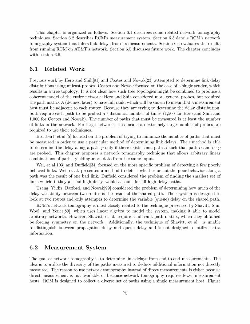
This chapter is organized as follows: Section 6.1 describes some related network tomographytechniques. Section 6.2 describes RCM’s measurement system. Section 6.3 details RCM’s networktomography system that infers link delays from its measurements. Section 6.4 evaluates the resultsfrom running RCM on AT&T’s network. Section 6.5 discusses future work. The chapter concludeswith section 6.6.

6.1 Related Work

Previous work by Hero and Shih[91] and Coates and Nowak[23] attempted to determine link delaydistributions using unicast probes. Coates and Nowak focused on the case of a single sender, whichresults in a tree topology. It is not clear how such tree topologies might be combined to produce acoherent model of the entire network. Hero and Shih considered more general probes, but requiredthe path matrix A (defined later) to have full rank, which will be shown to mean that a measurementhost must be adjacent to each router. Because they are trying to determine the delay distribution,both require each path to be probed a substantial number of times (1,500 for Hero and Shih and1,000 for Coates and Nowak). The number of paths that must be measured is at least the numberof links in the network. For large networks, this means an extremely large number of probes arerequired to use their techniques.

Breitbart, et al.[5] focused on the problem of trying to minimize the number of paths that mustbe measured in order to use a particular method of determining link delays. Their method is ableto determine the delay along a path p only if there exists some path α such that path α and α · pare probed. This chapter proposes a network tomography technique that allows arbitrary linearcombinations of paths, yielding more data from the same input.

Wei, et al[103] and Duffield[34] focused on the more specific problem of detecting a few poorlybehaved links. Wei, et al. presented a method to detect whether or not the poor behavior along apath was the result of one bad link. Duffield considered the problem of finding the smallest set oflinks which, if they all had high delay, would account for all high-delay paths.

Tsang, Yildiz, Barford, and Nowak[99] considered the problem of determining how much of thedelay variability between two routes is the result of the shared path. Their system is designed tolook at two routes and only attempts to determine the variable (queue) delay on the shared path.

RCM’s network tomography is most closely related to the technique presented by Shavitt, Sun,Wool, and Yener[89], which uses linear algebra to model the system, making it able to modelarbitrary networks. However, Shavitt, et al. require a full-rank path matrix, which they obtainedbe forcing symmetry on the network. Additionally, the technique of Shavitt, et al. is unableto distinguish between propagation delay and queue delay and is not designed to utilize extrainformation.

6.2 Measurement System

The goal of network tomography is to determine link delays from end-to-end measurements. Theidea is to utilize the diversity of the paths measured to deduce additional information not directlymeasured. The reason to use network tomography instead of direct measurements is either becausedirect measurement is not available or because network tomography requires fewer measurementhosts. RCM is designed to collect a diverse set of paths using a single measurement host. Figure

75

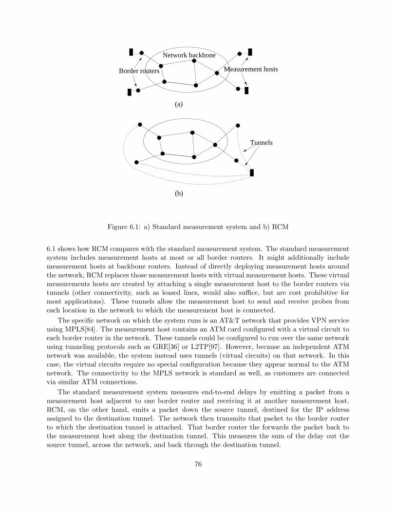
Measurement hosts

Network backbone

Border routers

Tunnels

(a)

(b)

Figure 6.1: a) Standard measurement system and b) RCM

6.1 shows how RCM compares with the standard measurement system. The standard measurementsystem includes measurement hosts at most or all border routers. It might additionally includemeasurement hosts at backbone routers. Instead of directly deploying measurement hosts aroundthe network, RCM replaces those measurement hosts with virtual measurement hosts. These virtualmeasurements hosts are created by attaching a single measurement host to the border routers viatunnels (other connectivity, such as leased lines, would also suffice, but are cost prohibitive formost applications). These tunnels allow the measurement host to send and receive probes fromeach location in the network to which the measurement host is connected.

The specific network on which the system runs is an AT&T network that provides VPN serviceusing MPLS[84]. The measurement host contains an ATM card configured with a virtual circuit toeach border router in the network. These tunnels could be configured to run over the same networkusing tunneling protocols such as GRE[36] or L2TP[97]. However, because an independent ATMnetwork was available, the system instead uses tunnels (virtual circuits) on that network. In thiscase, the virtual circuits require no special configuration because they appear normal to the ATMnetwork. The connectivity to the MPLS network is standard as well, as customers are connectedvia similar ATM connections.

The standard measurement system measures end-to-end delays by emitting a packet from ameasurement host adjacent to one border router and receiving it at another measurement host.RCM, on the other hand, emits a packet down the source tunnel, destined for the IP addressassigned to the destination tunnel. The network then transmits that packet to the border routerto which the destination tunnel is attached. That border router the forwards the packet back tothe measurement host along the destination tunnel. This measures the sum of the delay out thesource tunnel, across the network, and back through the destination tunnel.

76

One disadvantage of using tunnels is that the raw data is not meaningful to operations. Whenusing a standard measurement system, each measured delay equals the end-to-end delay observedbetween two border routers. Using tunnels means that each measured delay includes artificialdelays from both the outbound and inbound tunnels. Previously, analysis was necessarily only todetermine link delays. Now, analysis is required to determine end-to-end delays as well. Even if anISP only wanted to monitor changes from a baseline, the tunnel delays must still be determined,because a change in a measured delay could be the result of a change in the network or in the delayacross one of the tunnels. This is a minor drawback, as analysis is already required to detect whichlinks are responsible for changes in end-to-end delays. Once link delays have been determined,end-to-end delays can be determined by subtracting the tunnel delays from the raw measurements.

Using tunnels somewhat complicates the analysis, as each measurement now includes two morepseudo-links (the tunnels added at the beginning and end of each path). Moreover, all paths becomeloops instead of paths. In order to determine link delays, the paths must remain sufficiently“diverse”. It will be shown in Section 6.3 that the introduction of these pseudo-links does notadversely affect path diversity.

The drawbacks thus far are minor, in that they can be handled by analysis techniques describedbelow. One potential issue that can not be dealt with by analysis techniques is that RCM replacesthe need to deploy measurement systems with the need to deploy tunnels. The ISP must still deploythe tunnels to a diverse set of routers. Is deploying tunnels better than deploying measurementhosts? Using tunnels instead of measurements hosts has three advantages: deploying tunnels issimpler than deploying measurement hosts, using one measurement host allows more coordinationof the measurements, and collecting the raw measurements for analysis is simplified.

Deploying tunnels is much cheaper and faster than deploying measurement hosts. Tunnels canbe deployed by changing configurations. As mentioned in the overview, adding a measurement hostnext to a router requires obtaining approval to install a measurement host, procuring the hardwareand software for the host, shipping that hardware to the POP where the router is located, andconfiguring the host for its particular location. The alternative of using existing hosts requiresthe availability of compatible hosts with sufficient resources to host the measurement software andgaining permission to use said hosts. For the particular AT&T network on which the system resides,deploying a new ATM tunnel follows nearly the same process as adding a customer, which is doneon a daily basis. Tunnels can be deployed in minutes with no effect on the network. Hardwaredeployment can take weeks or longer. Using existing hosts has the additional danger of affectingother programs running on that host. Using tunnels also allows flexibility in the placement of themeasurement host. For the deployed system, the host was placed in the network operations center,where it is easily serviced and managed. Remote measurements hosts must be placed in a POP,which may have limited or no on-site staff, greatly complicating maintenance.

Using tunnels means that the measurement packets are sent and received by the same host.This has additional benefits beyond the obvious advantage of avoiding the problem of clock syn-chronization. For example, fine-grained scheduling allows the probes to be timed to minimize theload on routers and links. While such fine-grained scheduling is straight-forward within a singlehost, it would be difficult to do across multiple hosts.

Because data collection is now done by a single host, the data is stored completely on thathost. Thus, the raw data does not need to be transferred to a single host to do analysis. Thismeans the network load induced by raw data transfers or distributed algorithms can be avoidedor flexibly scheduled to minimize the effect on the network. Analysis of the data can take place

77

3

1

p p1

2p

l

Figure 6.2: Example set of measured paths useful for determining link l1.

instantaneously, as complete data is available to the measurement host at all times. This meansthe results (generally much smaller than the raw data) can be available quickly and that the datacollection can adapt to measurements more rapidly.

6.3 Tomography Technique

Conceptually, RCM’s network tomography technique works by taking linear combinations of pathsto determine delays of links not directly measured. Consider the set of paths shown in Figure 6.2.The delay across link l1 should be the sum of the delay across paths p1 and p3 minus the delayacross path p2. These linear combinations can be arbitrary complex.

Before defining the technique, some notation is necessary. Denote the (directed) links as L ={lj} and the paths as P = {pi}, where each pi is a subset of L. Define the path matrix, A, as the‖P‖ by ‖L‖ matrix given by Aij = ‖pi ∩ {lj}‖. If all the paths are simple, then A is a booleanmatrix.

RCM’s network tomography technique expands on the technique presented by Shavitt, Sun,Wool, and Yener[89], which solved for the delay vector d from the measured delays b using thefollowing equation:

Subject to Ad − e = bMinimize ‖e‖2

(6.1)

Equation 6.1 is solvable using least-squares errors techniques[98] if A is full-rank. Unfortunately,A is never full-rank unless each router in the topology is the end-point of a measured path. Thiswould imply a measurement host is next to each router, making network tomography techniquesunnecessary.

Lemma 1 rank(A) ≤ ‖L‖ − ‖I‖, where I is the set of routers within the network which are notthe endpoint of any measured path.

Proof: For all routers along a measured path except the endpoints, the in-degree equals theout-degree. That is, for x ∈ I, the in-degree equals the out-degree for all measured paths. Let y bea router which is the endpoint of at least one measured path. For any x ∈ I, let px denote a pathfrom x to y. The path px cannot be expressed as a linear combination of measured paths, since thein-degree of x does not equal the out-degree. Each path px corresponds to a vector vx specifying

78

the links in the path. Let V = {vx|x ∈ I}. V is linearly independent for the same reason that vx

is linear independent from the measured paths. Therefore, rank(A) ≤ ‖L‖ − ‖V ‖ = ‖L‖ − ‖I‖.

Shavitt, et al. avoided this problem by assuming that link delays are symmetric. While oftentrue, it limits the ability to model arbitrary networks. Shavitt, et al. additionally allowed negativelink delays and did not distinguish between propagation delay and queue delay. RCM addresseseach of these issues.

6.3.1 Algorithm Inputs and Outputs

The input to the algorithm is a set of one-way delay measurements for a set of paths over a timeperiod of interest. For the purposes of the algorithm, this set of paths need not be measuredfrom a single measurement host. Thus, the algorithm will work when a standard measurementsystem is employed. Each path in the input is measured a medium number of times (twenty in theimplementation). The output should be the delay across each (directed) link within the network.This chapter will present the algorithm in three steps: conceptual form, basic mathematical form,and relaxed mathematical form. The algorithm does not use computed models from previous timeperiods, making the algorithm stateless.

Note that the paths over which the delay measurements are taken are assumed to be known.The implementation does this by examining the OSPF configuration. At the time of writing, thesystem does not have access to live OSPF data. As such, network events such as a link outage androuter maintenance cause measurements to take different paths than the one specified. Althoughsuch events are rare, the resulting input flaws usually result in RCM being unable to model thesystem. This problem is solvable by listening to OSPF announcements using technologies such asRoute Explorer[44], RouteDynamics[85], or OSPF Monitor[88]. Adding such a monitor is left forfuture work.

This assumption is also adversely affected by equal-cost multi-path (ECMP). With ECMP,knowing the routing state is insufficient, as the routing state gives a set of possible paths thata packet can take. The decision of which path each packet should take is left to the forwardingengine. Its decisions may be measured by traceroute[46] on non-tunneled networks. On manytunneled networks, including RCM’s, the tunnel appears as a single hop, making traceroute unableto identify which particular path is used. Network tomography on a network with large amountsof ECMP that cannot be resolved by traceroute is discussed in Section 6.5. For the network ofinterest, measurements whose paths are unknown are discarded. Because ECMP is rare, discardingthese measurements does not decrease the usefulness of the results.

6.3.2 Algorithm Motivation

The delay across a link has two components: the propagation delay (p) and the queue delay (q). Thepropagation delay is constant over medium time frames (minutes to days), while the queue delayvaries by the millisecond. Given a set of measurements for a particular path, the minimum observeddelay corresponds to the smallest total queue delay seen for that path. Presuming congestion istransient and not endemic, something for which all ISPs strive, the smallest observed queue delayshould be nearly zero. This means the minimum measured delay should represent only propagationdelay. The average measured delay corresponds to the sum of the propagation delay and the averagequeue delay.

79

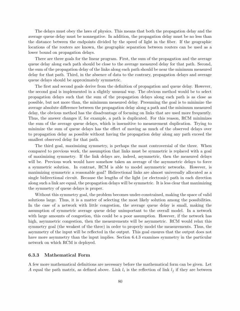
The delays must obey the laws of physics. This means that both the propagation delay and theaverage queue delay must be nonnegative. In addition, the propagation delay must be no less thanthe distance between the endpoints divided by the speed of light in the fiber. If the geographiclocations of the routers are known, the geographic separation between routers can be used as alower bound on propagation delays.

There are three goals for the linear program. First, the sum of the propagation and the averagequeue delay along each path should be close to the average measured delay for that path. Second,the sum of the propagation delay of the links along each path should be near the minimum measureddelay for that path. Third, in the absence of data to the contrary, propagation delays and averagequeue delays should be approximately symmetric.

The first and second goals derive from the definition of propagation and queue delay. However,the second goal is implemented in a slightly unusual way. The obvious method would be to selectpropagation delays such that the sum of the propagation delays along each path is as close aspossible, but not more than, the minimum measured delay. Presuming the goal is to minimize theaverage absolute difference between the propagation delay along a path and the minimum measureddelay, the obvious method has the disadvantage of focusing on links that are used more frequently.Thus, the answer changes if, for example, a path is duplicated. For this reason, RCM minimizesthe sum of the average queue delays, which is insensitive to measurement duplication. Trying tominimize the sum of queue delays has the effect of moving as much of the observed delays overto propagation delay as possible without having the propagation delay along any path exceed thesmallest observed delay for that path.

The third goal, maximizing symmetry, is perhaps the most controversial of the three. Whencompared to previous work, the assumption that links must be symmetric is replaced with a goalof maximizing symmetry. If the link delays are, indeed, asymmetric, then the measured delayswill be. Previous work would have somehow taken an average of the asymmetric delays to forcea symmetric solution. In contrast, RCM is able to model asymmetric networks. However, ismaximizing symmetric a reasonable goal? Bidirectional links are almost universally allocated as asingle bidirectional circuit. Because the lengths of the light (or electronic) path in each directionalong such a link are equal, the propagation delays will be symmetric. It is less clear that maximizingthe symmetry of queue delays is proper.

Without this symmetry goal, the problem becomes under-constrained, making the space of validsolutions large. Thus, it is a matter of selecting the most likely solution among the possibilities.In the case of a network with little congestion, the average queue delay is small, making theassumption of symmetric average queue delay unimportant to the overall model. In a networkwith large amounts of congestion, this could be a poor assumption. However, if the network hashigh, asymmetric congestion, then the measurements will be asymmetric. RCM would relax thissymmetry goal (the weakest of the three) in order to properly model the measurements. Thus, theasymmetry of the input will be reflected in the output. This goal ensures that the output does nothave more asymmetry than the input implies. Section 6.4.3 examines symmetry in the particularnetwork on which RCM is deployed.

6.3.3 Mathematical Form

A few more mathematical definitions are necessary before the mathematical form can be given. LetA equal the path matrix, as defined above. Link li is the reflection of link lj if they are between

80

the same pair of routers but in opposite directions. Let R be an |L| x |L| symmetric matrix, givenby:

Rij =

1 if li is the reflection of lj1 if i = j and there is no reflection of li0 otherwise

(6.2)

Each row and column in R contains exactly one non-zero entry. Such a matrix is called apermutation matrix, because multiplying R by a vector x permutes the vector. In this case, if p isthe propagation delay across each link, then Rp is the propagation delay across the reverse of eachlink. Thus ‖Rp − p‖1 = ‖(R − I)p‖1 is twice the sum of the asymmetry of the propagation delayof each link. For simplicity, define R = R − I.

Let the vectors bmin and b respectively correspond to the minimum and average measured delayfor each path in the time frame of consideration. Let p0 be the lower-bound on propagation delaysthat results from geographic separation. If the geographic locations are not known, set p0 = 0(the effect of lacking geographic information will be examined in Section 6.4.1). The output of thetechnique is two vectors, p and q, respectively specifying the propagation delay and average queuedelay for each link in the network.

Given these definitions, the basic form of the network tomography technique is:

Subject to Ap ≤ bmin

p ≥ p0, q ≥ 0

Goal 1 Minimize ‖A(p + q) − b‖2

Goal 2 Minimize C‖q‖1 + ‖Rp‖1 + ‖Rq‖1

(6.3)

The first goal is solved as a least square error problem using the Householder QR factorization[98]to project b to range(A). This technique ignores the lower bounds on p and q. Goal 2 is solvedassuming the result from goal 1. The constant C specifies the relative weight of queue delay andantisymmetry. As C increases, the system becomes more willing to increase antisymmetry to reducequeue delay. C = ∞ is equivalent to minimizing ‖q‖1 and, subject to that minimum, minimizing‖Rp‖1 + ‖Rq‖1. Figure 6.3 shows the antisymmetry and total queue delay for different values of Cfor the measured network. The behavior is similar for values of C between 1 and 106. For C = 107,the antisymmetry increases from 180 to 70,000 to accommodate a decrease of 0.016 in the queuedelay. This focuses undesirably on minimizing queue delay without regard to antisymmetry. LargeC values have the additional disadvantage of magnifying numerical errors. After experimentation,C = 100 was selected for the network in consideration. This still strongly favors a decrease in queuedelay, as it allows the linear program solver to accept an increase of 100 milliseconds in asymmetryin order to reduce the total queue delay by 1 millisecond. As implied by Figure 6.3, other valuesaround C = 100 would yield similar results.

The problem with the basic form of the system given in equation 6.3 is that measurement errorscan result in the system having no solution. A small measurement error can result in the basic formmissing a reasonable solution because the delays are slightly below the lower bounds. Equation 6.3cannot distinguish between that and no remotely reasonable solution existing. For this reason, thebasic form must be relaxed by introducing slack variables pe and qe. These slack variables allow thepropagation and queue delays to be less than the specified lower bounds. The relaxed formulationis:

81

150

160

170

180

190

200

210

220

0.0001 0.01 1 100 10000 1e+06 1e+08

Sum

of V

alue

s (a

rbitr

ary

units

)

Constant

Effect of Constant Values

Total Queue DelayAntisymmetry

Figure 6.3: Effect of constant C on total queue delay and antisymmetry.

Subject to Ap ≤ bmin

p + pe ≥ p0, q + qe ≥ 0pe ≥ 0, qe ≥ 0

Goal 1 Minimize ‖A(p + q) − b‖2

Goal 2 Minimize ‖pe‖1 + ‖qe‖1

Goal 3 Minimize C‖q‖1 + ‖Rp‖1 + ‖Rq‖1

(6.4)

The relaxation goal (goal 2) is solvable using linear programming. This form has the advantageof quantifying the violation: ‖pe‖1 + ‖qe‖1. Large violations (more than 0.1 milliseconds total),based on experience, reflect errors in the inputs, either the measurements, the geographic separationbound, or the path matrix. This will be discussed in more detail below.

6.3.4 Requirements

For RCM’s network tomography technique to function properly, a few requirements on the inputare necessary. The first requirement is obvious: RCM cannot determine the delay across any linkthat is not in at least one measured path. This requirement is unavoidable, as the measurementscontain no information about links not along any measurement path. Despite being obvious andunavoidable, it is an important consideration when selecting the set of paths to measure.

The less obvious requirement is that the measured paths must be “diverse enough”. Diversitywill be defined more precisely in a moment, but the basic form of diversity is that no internal routercan have degree two in the undirected form of the network. Consider the two cases shown in Figure6.4. Any path will either traverse both links or traverse neither link, giving low path diversity.If a path traverses both links, then packets will be take 10 milliseconds to traverse both links in

82

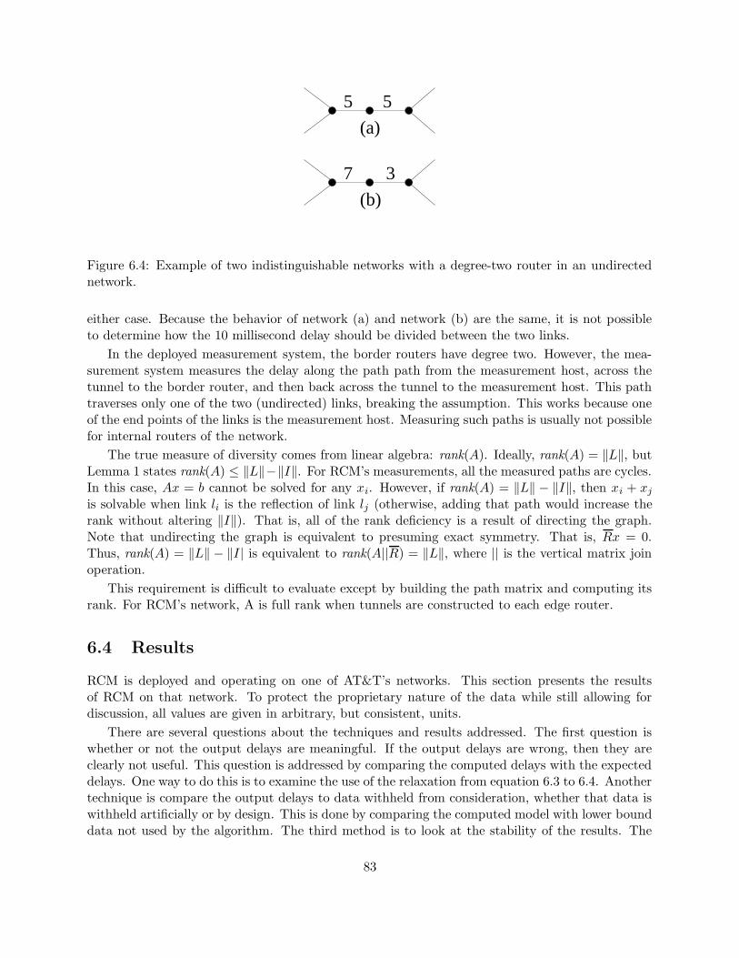
(b)

7 3

5 5

(a)

Figure 6.4: Example of two indistinguishable networks with a degree-two router in an undirectednetwork.

either case. Because the behavior of network (a) and network (b) are the same, it is not possibleto determine how the 10 millisecond delay should be divided between the two links.

In the deployed measurement system, the border routers have degree two. However, the mea-surement system measures the delay along the path path from the measurement host, across thetunnel to the border router, and then back across the tunnel to the measurement host. This pathtraverses only one of the two (undirected) links, breaking the assumption. This works because oneof the end points of the links is the measurement host. Measuring such paths is usually not possiblefor internal routers of the network.

The true measure of diversity comes from linear algebra: rank(A). Ideally, rank(A) = ‖L‖, butLemma 1 states rank(A) ≤ ‖L‖−‖I‖. For RCM’s measurements, all the measured paths are cycles.In this case, Ax = b cannot be solved for any xi. However, if rank(A) = ‖L‖ − ‖I‖, then xi + xj

is solvable when link li is the reflection of link lj (otherwise, adding that path would increase therank without altering ‖I‖). That is, all of the rank deficiency is a result of directing the graph.Note that undirecting the graph is equivalent to presuming exact symmetry. That is, Rx = 0.Thus, rank(A) = ‖L‖ − ‖I| is equivalent to rank(A||R) = ‖L‖, where || is the vertical matrix joinoperation.

This requirement is difficult to evaluate except by building the path matrix and computing itsrank. For RCM’s network, A is full rank when tunnels are constructed to each edge router.

6.4 Results

RCM is deployed and operating on one of AT&T’s networks. This section presents the resultsof RCM on that network. To protect the proprietary nature of the data while still allowing fordiscussion, all values are given in arbitrary, but consistent, units.

There are several questions about the techniques and results addressed. The first question iswhether or not the output delays are meaningful. If the output delays are wrong, then they areclearly not useful. This question is addressed by comparing the computed delays with the expecteddelays. One way to do this is to examine the use of the relaxation from equation 6.3 to 6.4. Anothertechnique is compare the output delays to data withheld from consideration, whether that data iswithheld artificially or by design. This is done by comparing the computed model with lower bounddata not used by the algorithm. The third method is to look at the stability of the results. The

83

0

500

1000

1500

2000

2500

3000

06/26 07/03 07/10 07/17 07/24 07/31 08/07 08/14 08/21 08/28

Tot

al V

iola

tion

(arb

itrar

y un

its)

Date

Violation over time

Figure 6.5: Sum of constraints violations for each time period

variation between time periods should be commensurate with the variation in the measurements.Otherwise, the system is likely to be suffering from numeric instability.

The second question is the efficacy of the method. That is, is it able to assign delay changes toa particular link? If not, the system is able only to determine when there might be a problem inthe network and not be able to pinpoint the problem. In fact, the system would not even be ableto conclusively distinguish between delays changing in the ATM network and delays changing inthe MPLS network, leading to false alarms.

The last question is how reasonable the symmetry goal is for this particular network. RCMassumes symmetry in the absence of data to the contrary. If the resulting model routinely containslarge amounts of asymmetry, then this may be a poor assumption.

For the network on which the system is deployed, the measured delays vary little over shorttime frames (milliseconds). The variation is is the order of magnitude of the expected error of themeasurement system. As such, the network has little actual queue delay. This small queue delayis reflected in RCM’s output. While small queue delay is a good property for a network to have,it makes meaningful analysis of queue delay difficult at best. Because queue delays are all nearlyzero, this analysis focuses on propagation delays.

6.4.1 Meaningful Results

As mentioned, the first item to consider when looking if the results are reasonable is the extentto which the slack variables in equation 6.4 are employed. Figure 6.5 shows the total violation(‖pe‖1 + ‖qe‖1) for each time period over two months. The violation is nonzero in only 113 ofthe 7,722 time periods shown (1.5%). There are two known causes for non-zero violation: timedivision and routing knowledge. Most of the cases of non-zero violation result from the way inwhich time is divided. Currently, time is modeled into ten minute periods. If the behavior of the

84

network changes in that ten minute time period, then the algorithm is effectively trying to modeltwo different behaviors with a single model. This difficult task can result in a solution with non-zeroviolation. Properly dividing time into epochs of similar behavior would eliminate such problems.That problem is tangential to the problem determining delays once time has been properly dividedand is left to future work.

Persistent non-zero violations can result from changes to the network. As mentioned above,the current system does not include an OSPF monitor. Instead, it uses manual dumps taken fromOSPF. If a link becomes disconnected or a router is taken offline for maintenance, the topologyinformation becomes incorrect. This results in a difference between the paths taken by the mea-surement packets and what the system believes them to be. Several existing systems are able tomonitor OSPF[44, 85, 88]. Changes in topology are much more rare than changes in link delaysOf the 113 time periods with non-zero violation, 95 are the result of time division problems and 18result from topology changes.

Note that when the violation is zero, RCM produces the same result as Equation 6.2 would.When the violation is non-zero, Equation 6.2 would yield no solution. Because it uses the relaxedform given in Equation 6.4, RCM is able to produce a potential model of the system. The non-zero violation reports that the produced model is inaccurate and gives a quantitive value of itsinaccuracy.

Another question to address is the how well the results correspond to unknown data. Foreach link in the network, there is an estimate of the number of “routing miles” traversed by thatlink. Routing miles are computed by looking at the network beneath the MPLS network andapproximating the actual number of miles of fiber a packet must travel to traverse a link. Becauseit is an approximation, routing miles data is not used to raise the lower bound on propagationdelays. Despite not being an input, the routing miles should closely correspond to the propagationdelay. Figure 6.6 shows the relationship between routing miles and the computed propagationdelay for every time period on July 31, 2004. For most links, routing miles correspond to thecomputed propagation delay: 83% of the computed propagation delays are within 100 units (5%of the maximum propagation delay) of the delay implied by routing miles. Routing miles arecomputed with knowledge of the network and limited knowledge of routing, while the propagationdelay is computed from measurements. Therefore, when routing miles diverge from the computedpropagation delay, it is not clear which value is more likely to be in error. In any case, RCM yieldspropagation delays that closely correspond to routing miles for most links.

Another comparison with withheld data can be performed by artificially withholding the geo-graphic knowledge. This also models the case where a user is trying to use network tomographyto determine link delays, as a user is unlikely to have geographic knowledge for all routers inthe network. Figure 6.7 compares the computed propagation delays with and without geographicknowledge. Although 40% of the computed delays changed when geographic knowledge was re-moved, only 4% changed significantly2. All significant changes occurred in links whose propagationdelay is less than seven units. The computed propagation delay of long links is not affected by theremoval of the geographic knowledge. Since the resulting propagation delays violate the geographicknowledge, the geographic knowledge is helpful. However, the system is not heavily dependenton these bounds. Geographic knowledge improves the accuracy of computed propagation delaysprimarily for links with a low propagation delay.

2Significant is defined as a move of at least 2% and at least 0.1 units. This definition falls within an large gap:

85

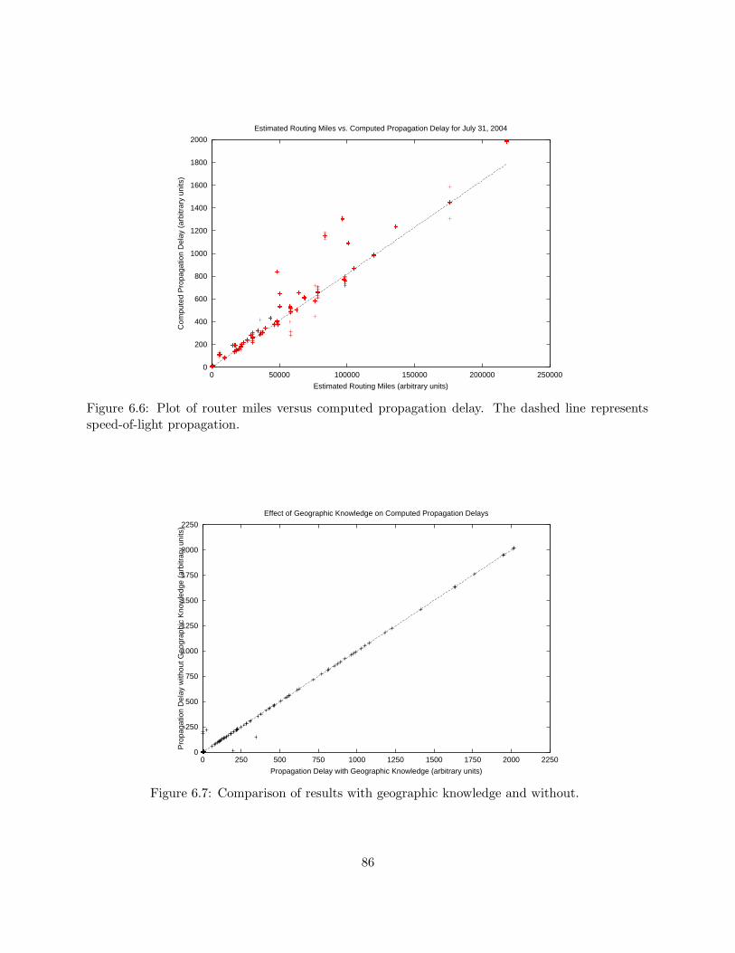
0

200

400

600

800

1000

1200

1400

1600

1800

2000

0 50000 100000 150000 200000 250000

Com

pute

d P

ropa

gatio

n D

elay

(ar

bitr

ary

units

)

Estimated Routing Miles (arbitrary units)

Estimated Routing Miles vs. Computed Propagation Delay for July 31, 2004

Figure 6.6: Plot of router miles versus computed propagation delay. The dashed line representsspeed-of-light propagation.

0

250

500

750

1000

1250

1500

1750

2000

2250

0 250 500 750 1000 1250 1500 1750 2000 2250

Pro

paga

tion

Del

ay w

ithou

t Geo

grap

hic

Kno

wle

dge

(arb

itrar

y un

its)

Propagation Delay with Geographic Knowledge (arbitrary units)

Effect of Geographic Knowledge on Computed Propagation Delays

Figure 6.7: Comparison of results with geographic knowledge and without.

86

140

145

150

155

160

165

170

175

180

185

07/2500:00

07/2512:00

07/2600:00

07/2612:00

07/2700:00

07/2712:00

07/2800:00

Com

pute

d P

ropa

gatio

n D

elay

(ar

bitr

ary

units

)

Time

Computed Propagation Delays for Sample Link

Figure 6.8: Stability of computed propagation delay over three days.

Besides constraint violation and comparison with withheld data, another expected behavior isthat propagation delays should be stable. Thus, the propagation delay across a link might changeoccasionally when the link is rerouted within the underlying network, but such reroutes should berare and result in sharp measurement changes. Outside of these abrupt changes, the propagationdelay should not change. Some variation in the computed propagation delay is expected due tounavoidable measurement errors, but such variations should be minimal. Because the algorithm isstateless, all stability is a result of the underlying algorithm. Figure 6.8 shows that the computedpropagation delay for a particular link over three days. Although this link’s computed propagationdelay changes little over these three days, and yet observed delays along some paths changedsignificantly. These changes, discussed in Section 6.4.2, were determined to be the result of changesin the delay over other links. In the face of the network changing, the computed propagation delayacross this link is stable, varying by no more than 20 units from the median of 163.2 and rarelymore than 3 units. This link’s stability is representative of all the links in the network.

6.4.2 Efficacy

Figure 6.9 shows the measured delay between a pair of tunnels (border routers) over three days. Atapproximately midnight on July 26, the delay changed from 2600 to 2800, dropping back to around2600 about 21 hours later then dropping to 2400 six hours after that. As the routing of this pathdid not change, these fluctuations must be the result of a change in the propagation delay acrosslinks in the path. Notice, however, that the measured delays in each of these modes of behaviorare are nearly constant, with only six measurements (out of more than 30,000) varying more than2% from the norm of the current mode. This implies that most changes in observed delays are theresult of propagation delays of the links used and not a result of congestion (queue delay).

the smallest significant move was 137% and 4.0 units.

87

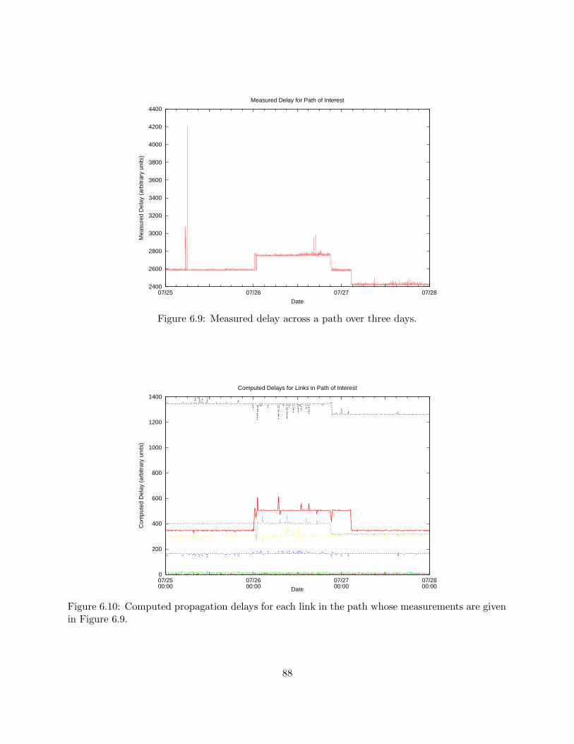
2400

2600

2800

3000

3200

3400

3600

3800

4000

4200

4400

07/25 07/26 07/27 07/28

Mea

sure

d D

elay

(ar

bitr

ary

units

)

Date

Measured Delay for Path of Interest

Figure 6.9: Measured delay across a path over three days.

0

200

400

600

800

1000

1200

1400

07/2500:00

07/2600:00

07/2700:00

07/2800:00

Com

pute

d D

elay

(ar

bitr

ary

units

)

Date

Computed Delays for Links in Path of Interest

Figure 6.10: Computed propagation delays for each link in the path whose measurements are givenin Figure 6.9.

88

Figure 6.10 shows how the RCM assigns delay to the propagation delays of the links alongthe path measured. It shows that the rise from 2600 to 2800 is due to a change in the delayacross the link represented by the solid line. The drop back to 2600 from 2800 that occurred 21hours later is not, in fact, that the link returned to its previous propagation delay, but rather thepropagation delay over the two links represented by the top two dashed lines changed. These twolines correspond to the two tunnels used by the measurement. Thus, despite the measurementsreturning to nearly the original level, the actual delays across the path in the MPLS network remain200 higher than normal. The delays across the MPLS network did not return to normal levels foranother six hours. The change in the delay of the link in the MPLS network was confirmed, usingother means, as a reroute of the MPLS link in the network upon which the MPLS network runs.

6.4.3 Symmetry

As mentioned above, perhaps the most controversial piece of RCM’s network tomography tech-nique is the symmetry goal of minimizing ‖Rp‖1 + ‖Rq‖1. Without this term, the system isunder-constrained. Thus, this term has the effect of selecting among a set of otherwise equally-good solutions. A valid question is whether or not a symmetric solution is more likely than anon-symmetric one. Regardless, the solution is improved over previous techniques that forced sym-metry without respect for the symmetry of the measurements. RCM allows asymmetric link delayswhen the measurements are asymmetric. The symmetry term has the effect of avoiding artificialsymmetry not implied by the measurements.

To determine whether or not this is a reasonable goal for this network, consider the symmetryof the input and output data. If the measurements are symmetric and can be modeled by nearlysymmetric link delays, then maximizing symmetry is probably a reasonable goal. On the other hand,if asymmetry in rampant in either the input or output data, then selecting the most symmetricsolution may not be the best method. Note that if the output is not symmetric, then previoustechniques that forced exact symmetry would also not be able to model the system well.

Figure 6.11 shows the symmetry of the measured delays for one day. This figure plots themeasured delay of the forward path against the measured delay of the reverse path, where delays areaveraged over twenty measurements performed over ten minutes. Because routing on this networkis symmetric for most paths, the measured delays are, for the most part, nearly symmetric. Whenmultiple paths exist with equal costs between two border routers, the forward and reverse pathsare assigned one of the equal-cost paths pseudo-randomly. This can result in a forward path thatdiffers from the reverse path, resulting in asymmetric path delays even if link delays are symmetric.ECMP is responsible for all the data points where the forward and reverse path delays differ bymore than 200 units.

Figure 6.12 shows the symmetry of the computed propagation delays. The computed propaga-tion link delays are nearly symmetric. More than half (55%) of the computed propagation delaysare exactly symmetric. 93% of the computed propagation link delays are symmetric within either5% or 2 units, although a few links are strongly asymmetric: 0.06% of the computed propagationdelays are antisymmetric by more than 100 units. Thus, almost all of the output propagation delaysare nearly symmetric.

Because the measured delays are symmetric except when routing is not symmetric and becausethe measurements can be modeled with nearly symmetric delays, maximizing symmetry appears tobe a reasonable goal. This does not rule-out asymmetric delays, but combined with the fact that

89

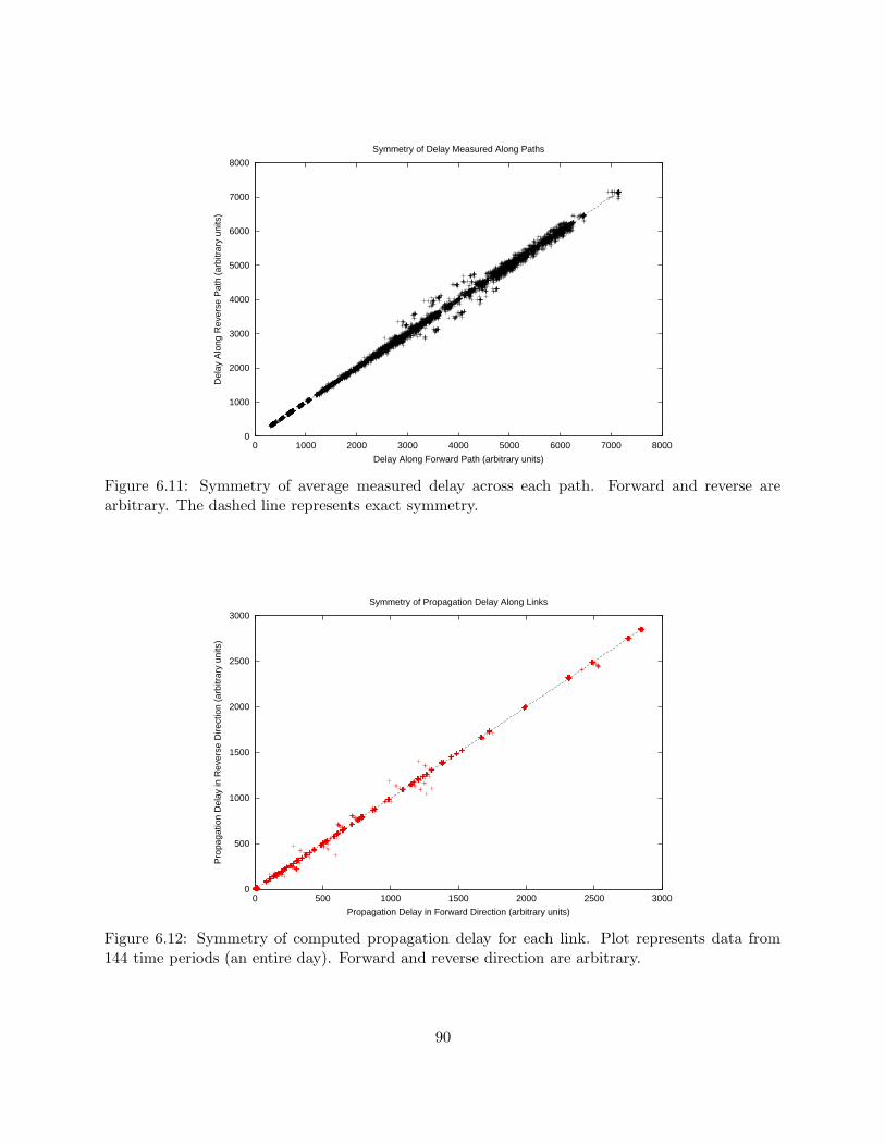
0

1000

2000

3000

4000

5000

6000

7000

8000

0 1000 2000 3000 4000 5000 6000 7000 8000

Del

ay A

long

Rev

erse

Pat

h (a

rbitr

ary

units

)

Delay Along Forward Path (arbitrary units)

Symmetry of Delay Measured Along Paths

Figure 6.11: Symmetry of average measured delay across each path. Forward and reverse arearbitrary. The dashed line represents exact symmetry.

0

500

1000

1500

2000

2500

3000

0 500 1000 1500 2000 2500 3000

Pro

paga

tion

Del

ay in

Rev

erse

Dire

ctio

n (a

rbitr

ary

units

)

Propagation Delay in Forward Direction (arbitrary units)

Symmetry of Propagation Delay Along Links

Figure 6.12: Symmetry of computed propagation delay for each link. Plot represents data from144 time periods (an entire day). Forward and reverse direction are arbitrary.

90

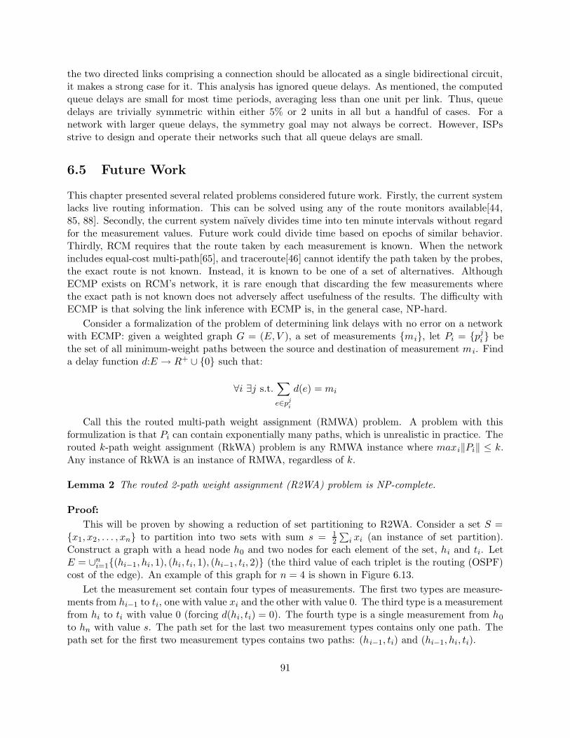
the two directed links comprising a connection should be allocated as a single bidirectional circuit,it makes a strong case for it. This analysis has ignored queue delays. As mentioned, the computedqueue delays are small for most time periods, averaging less than one unit per link. Thus, queuedelays are trivially symmetric within either 5% or 2 units in all but a handful of cases. For anetwork with larger queue delays, the symmetry goal may not always be correct. However, ISPsstrive to design and operate their networks such that all queue delays are small.

6.5 Future Work

This chapter presented several related problems considered future work. Firstly, the current systemlacks live routing information. This can be solved using any of the route monitors available[44,85, 88]. Secondly, the current system naıvely divides time into ten minute intervals without regardfor the measurement values. Future work could divide time based on epochs of similar behavior.Thirdly, RCM requires that the route taken by each measurement is known. When the networkincludes equal-cost multi-path[65], and traceroute[46] cannot identify the path taken by the probes,the exact route is not known. Instead, it is known to be one of a set of alternatives. AlthoughECMP exists on RCM’s network, it is rare enough that discarding the few measurements wherethe exact path is not known does not adversely affect usefulness of the results. The difficulty withECMP is that solving the link inference with ECMP is, in the general case, NP-hard.

Consider a formalization of the problem of determining link delays with no error on a networkwith ECMP: given a weighted graph G = (E, V ), a set of measurements {mi}, let Pi = {pj

i} bethe set of all minimum-weight paths between the source and destination of measurement mi. Finda delay function d:E → R+ ∪ {0} such that:

∀i ∃j s.t.∑

e∈pj

i

d(e) = mi

Call this the routed multi-path weight assignment (RMWA) problem. A problem with thisformulization is that Pi can contain exponentially many paths, which is unrealistic in practice. Therouted k-path weight assignment (RkWA) problem is any RMWA instance where maxi‖Pi‖ ≤ k.Any instance of RkWA is an instance of RMWA, regardless of k.

Lemma 2 The routed 2-path weight assignment (R2WA) problem is NP-complete.

Proof:

This will be proven by showing a reduction of set partitioning to R2WA. Consider a set S ={x1, x2, . . . , xn} to partition into two sets with sum s = 1

2

∑

i xi (an instance of set partition).Construct a graph with a head node h0 and two nodes for each element of the set, hi and ti. LetE = ∪n

i=1{(hi−1, hi, 1), (hi, ti, 1), (hi−1, ti, 2)} (the third value of each triplet is the routing (OSPF)cost of the edge). An example of this graph for n = 4 is shown in Figure 6.13.

Let the measurement set contain four types of measurements. The first two types are measure-ments from hi−1 to ti, one with value xi and the other with value 0. The third type is a measurementfrom hi to ti with value 0 (forcing d(hi, ti) = 0). The fourth type is a single measurement from h0

to hn with value s. The path set for the last two measurement types contains only one path. Thepath set for the first two measurement types contains two paths: (hi−1, ti) and (hi−1, hi, ti).

91

1

h h h h h

t t t t

0 1 2 3

1 2 3 4

4

2 2 2 2

1 1 1

111

1

Figure 6.13: Example, for n = 4, of graph constructed in proof of Lemma 2.

If a solution to the set partitioning problem exists, then let X ⊂ S with sum s. If xi ∈ X, thenlet d(hi−1, hi) = xi and d(hi−1, ti) = 0. If xi 6∈ X, then let d(hi−1, hi) = 0 and d(hi−1, ti) = xi.The resulting weighting makes the delay across (h0, h1, h2, . . . , hn) equal to

∑ni=1 d(hi−1, hi) =

∑

i|xi∈X xi = s. Thus, the delay function solves R2WA.

If a solution to the R2WA problem exists, then let X = {xi|d(hi−1, hi) = xi}. Because of thetwo measurements from hi−1 to ti, d(hi−1, hi) ∈ {0, xi}. Thus,

∑

i|xi∈X xi =∑n

i=1 d(hi−1, hi) = s.Therefore, the elements of X sum to s, and thus X solves the set partitioning problem.

Therefore, set partitioning is reducible to R2MA. Since set partitioning is NP-complete, R2MAis NP-complete.

Note that many restrictions of the problem do not change the result. The same proof will workwhen the problem is restricted to graphs of bounded degree (for bounds of at least four). The proofalso works if the input is a weighted digraph instead of a graph. Only minor revisions to the proofare necessary if all links have the same weight.

R2WA arises naturally from a network running OSPF with ECMP. Thus, Lemma 2 states thatoptimally assigning link delays in the presence of ECMP is intractable in the general case. It is notclear if the structure in real networks could be exploited or if heuristic or approximate techniquesare necessary. Determining link delays on a network with ECMP is left as future work.

6.6 Conclusions

This chapter describes RCM, a delay measurement and network tomography system to monitor end-to-end and link delays within a network using a single measurement host. RCM’s measurementsystem avoids the need for many measurement hosts by using tunnels to collect a diverse setof unicast measurements. This makes RCM easier, cheaper, and faster to deploy, operate, andmaintain.

RCM’s network tomography technique uses the measured delays to determine the propaga-tion and queue delay for each link. RCM’s network tomography technique works on an arbitrarytopology without needing to assume route symmetry or delay symmetry. RCM does not requirea measurement host at any internal nodes. It requires a few dozen probes of each path instead ofthousands, while still being able to determine both the propagation and queue delay of each link.

RCM cannot deal with equal-cost multi-path routes. It was shown that a generalized, exactform of the problem with ECMP is NP-complete. If path selection is done by looking at source anddestination IP addresses, then the path is consistent across measurements and may be measurable

92

using traceroute[46]. In a tunneled network where ECMP is common, heuristic techniques may benecessary.

RCM is deployed and operational on an AT&T’s network, from which results were presented.The computed delays correspond with expected behavior. In particular, the slack variables arerarely used, the delays match well with routing miles, the delays change little when geographicknowledge is removed, and the delays are stable over large time frames. In addition, when measureddelays shift due to a change in one or more link delays, the system is able to determine which linkdelays changed.

93

94

Chapter 7

Firewall Configuration and

Anonymous DNS1

From 1980 to 2000, the Internet grew from around 200 hosts to over 100 million[45]. As moreand more corporations connected their internal networks to the Internet, hackers discovered thattheir internal networks were not secure. While this poses limited risk if only employees are ableto access the network, once a company connects its network to the Internet, it becomes vulnerableto attacks from anyone on the Internet. To combat this without disconnecting their network fromthe Internet completely, corporations chose to limit their connectivity by deploying secure Internetgateways[15], which came to be known as “firewalls”. Firewalls examine the traffic between twoor more networks and selectively drop packets based on a set of rules. Recently, users have havestarted running software on their own host that acts as a firewall protecting access to just thathost, which have come to be known as “personal firewalls”.

Firewalls are an important first-line defense mechanism to limit network access to hosts andarguably the simplest and most popular form of network defense. How prevalent are firewalls?How securely are they configured? These questions provide important information about firewalldeployment on the Internet and could unveil potential security concerns. This chapter seeks answersto these questions and many other questions related to the deployment of these security defensemechanisms.

There are two basic philosophies when configuring a firewall: block by default and block byexception. In block by default, the default behavior is to not allow access to IP addresses behind thefirewall. The firewall allows access from the Internet to only particular services on particular hosts.This is common in higher-security networks, such as large corporate and government networks.In block by exception, only access to certain services is disabled. This is more common in lower-security networks, such as universities and residential ISPs. In these cases, the network operator isnot expected to block services, and, in fact, even limited blocking may be considered undesirableby network users. In block by default, the firewall administrator decides which services are usefulenough to specifically allow through the firewall. In block by exception, the firewall administratordecides which services pose a high enough security risk to block them at the firewall. Block by

1This chapter represents work with Dawn Song, published as “A Security Study of the Internet: An Analysis ofFirewall Behavior and Anonymous DNS” as a technical report at Carnegie Mellon University[9].

95

default is preferred by security experts and is more common in practice. An interesting questionone may ask is what percentage of IP addresses are beyond firewalls that block by default.

Another question related to the firewall analysis is to study the behavior of publicly accessibleservices. How many hosts are running public servers for different services? Do servers often runmultiple services? To increase security, it is recommended that administrators split public servicesacross hosts. If a host runs many services, compromising any of them compromises the entire host.By splitting the services between multiple hosts, the likelihood that any one host is compromisedis decreased and the impact of gaining access to a host is decreased, since taking the host offlineaffects only the services running on that host and services that depend on those services. Economicrealities, however, are such that operating more hosts increases hardware and administrative costs.Thus, many installations run multiple services on hosts to reduce costs.

Corporate networks are often separated from the Internet in naming as well. That is, hostnamesvalid within a corporate network may not resolve using domain name service (DNS) outside thatcorporation. This is known as “split DNS”. This chapter will focus on split reverse DNS, where,for example, 192.0.2.12 may reverse resolve to “inside.example.com” within a corporation, butreverse resolve to “host-192.0.2.12.example.com”, or some equally uninformative hostname, on theInternet. This provides a layer of obfuscation, as it makes it more difficult for an outside attackerto determine whether 192.0.2.12 is in use, much less what, if any, services it provides. Split DNSis somewhat analogous to firewalls for DNS: the Internet is allowed only partial access to internalDNS, usually limited to resolving external servers.

Split DNS is commonly implemented as assigning mechanically-generated hostnames to IP ad-dresses. This chapter focuses on mechanically-generated hostnames derived from the IP addresses,such as the example above. Such hostnames will be referred to as “anonymous DNS” because thehostname reveals little about the IP address. Split DNS is not the sole reason for anonymous DNS.For example, ISPs commonly do not give meaningful hostnames anywhere to the IP addresses oftheir residential customers. This chapter examines the prevalence of anonymous DNS and howmuch information is actually contained in reverse lookups. Most companies using anonymous DNSgenerate hostnames for all IP addresses they own, regardless of whether or not that IP address isin use.

Anonymous DNS affects attempts to estimate the number of hosts on the Internet that useDNS. Before firewalls were widely deployed, ping[75] could be combined with sampling to estimatethe number of hosts on the Internet. As firewalls grew in popularity, ping became increasingly inac-curate. This caused projects like ISC Internet Domain Survey[45] to use DNS instead. AnonymousDNS makes using DNS inaccurate. This chapter quantifies the error resulting from using DNS tocount hosts.

In summary, this chapter specifically addresses the following seven questions:

1. How prevalent are firewalls? What percentage of IP addresses are behind firewalls?

2. What do firewalls block? What services are commonly allowed and blocked by firewalls?

3. How much do firewalls block? What percentage of IP addresses are beyond firewalls that areblock by default?

4. How is firewall behavior correlated? Given a firewall blocks or allows a service, what otherservices is that firewall likely to block or allow?

96

5. What accessible services do hosts run?

6. How are running servers correlated? Given a server running a publicly available service, whatother publicly available services is it likely to run?

7. How prevalent are anonymous hostnames? What fraction of hosts and IP addresses haveanonymous hostnames?

To the best of the author’s knowledge, this work is the first attempt to systematically study thebehavior of firewalls and anonymous DNS on the Internet. This chapter proposes methodologiesand describes findings to address these questions. Many results are surprising and provide newinsights for understanding the deployment of security defense mechanisms on the Internet.

The rest of the chapter is organized as follows: Section 7.1 reviews previous work. Section 7.2details the methodology used. Section 7.3 presents the results, including answers to the questionsposed above. Section 7.4 gives the conclusions.

7.1 Previous Work

Most previous work which examined behavior of hosts on the Internet focused on the versionof services running on systems. Early previous work includes multiple RFCs: 669[29], 679[31],701[28], 702[30], 703[32], 751[55], 844[22], 847[104], and 876[92]. RFC 669, 679, 701, 702, and 703are periodic surveys looking at telnet server behavior to observe the deployment of the new telnetprotocol. RFC 751 is a survey that looks at how many mail daemons allow e-mail to unknownrecipients and how often a particular method to send e-mail is available. RFC 844 looks at thedeployment of ICMP. RFC 846 looks at the deployment of TCP. With the exception of RFC 751,all of these exclusively dealt with the rate of the deployment of a new service or protocol. Noneof these surveys included more than 400 hosts, because the Internet did not have more than 400hosts. That is small-scale when looked at in modern terms.

More recent work by Provos and Honeyman[82] studied the deployment of a new version ofSSH[107] after the discovery of a vulnerability in one version of the protocol. They scanned 400,000IP addresses at University of Michigan daily to determine the version of SSH server running onthe systems that responded (around 2,300 of the IP addresses). Again, they were focused on theversion of servers running, rather than looking at responsiveness of systems.

Several projects have used DNS to estimate the number of hosts on the Internet. They includeNetsizer[69], ISC Internet Domain Survey[45], and RIPE Region Hostcount[83].

7.2 Methodology

To analyze firewall behavior, IP addresses were probed for their responsiveness to particular services.Although some firewalls contain specific rules that allow particular external hosts special access totheir corporate network, this chapter focuses on the behavior of a request from a general host.This is the access that most hosts will see and it is not clear how these special hosts could bereasonably detected anyway. Two types of responsiveness are considered. The first category isa host responding to the service request. This does not mean that the host necessarily runs the

97

service, simply that no firewall blocks the request. The second category is a host listening for aservice. This means that no firewall blocks the request and the host offers initial access to theservice. The specific packet responses implying these two response types are service-specific andare detailed below.

Testing firewall behavior is composed of four pieces: selecting the services to test, selectingthe IP addresses to test, testing the IP addresses, and separating firewall responses from end-hostresponses. Because there are too many services to test all of them, a representative subset mustbe selected. Even if the set is limited to routed or allocated IP addresses, there are too many IPaddresses to test all of them. Thus, IP addresses must be sampled using a representative subset ofsufficient size to limit the error. Once the services and IP addresses are selected, the selected IPaddresses must be tested for responsiveness to those selected services. This requires defining whatresponsive means in the context of each service.

One unusual, and perhaps unexpected behavior, is that some firewalls respond to services forIP addresses beyond them. The goal is to test if IP addresses are responsive to the service. Ifthe firewall acts on behalf of the IP address, the IP address appears responsive, even though thefirewall does not allow the packet to reach the IP address. To remove these false positives, firewallresponses must be detected and removed.

7.2.1 Service Selection

It is not possible to test all possible services. There are 65,536 TCP ports and 65,536 UDP ports,too many to test with any level of detail in a reasonable time. Even limiting the search to portswith published services, there are almost 2000 of those listed in FreeBSD’s services file[81], still toomany to test responsiveness of for a reasonable number of IP addresses. Thus, a cross-section ofservices were selected. The seventeen services selected to test are listed in Table 7.1. These serviceswere selected for a variety of reasons:

1. Chargen (character generator)[77] is almost exclusively used for bad purposes. Security ex-perts suggest blocking it and there are few reasons not to block it.

2. DNS (domain name service)[64] is required for most other services to be useful. It is also aUDP service, unlike most of the services selected.

3. Echo[78] is similar to Chargen, but not as useful for bad purposes. Like Chargen, there arefew reasons not to block it.

4. Finger[109] is considered bad as it reveals user names. security experts suggest blocking it,but, unlike Chargen and Echo, it provides a useful service to end-users.

5. FTP (file transfer protocol)[80] is a popular service used primarily to publish files for publicdownload. FTP was selected for its popularity.

6. Gnutella[40] is a peer-to-peer (P2P) file sharing service. Given the potential for legal problemsdue to some uses of P2P services, Gnutella was expected to be blocked more often than otherservices.

98

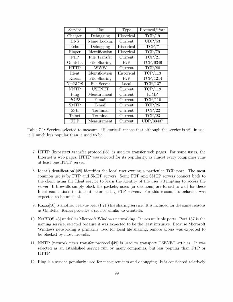
Service Use Type Protocol/Port

Chargen Debugging Historical TCP/19

DNS Name Lookup Current UDP/53

Echo Debugging Historical TCP/7

Finger Identification Historical TCP/79

FTP File Transfer Current TCP/21

Gnutella File Sharing P2P TCP/6346

HTTP WWW Current TCP/80

Ident Identification Historical TCP/113

Kazaa File Sharing P2P TCP/1214

NetBIOS File Server Local TCP/137

NNTP USENET Current TCP/119

Ping Measurement Current ICMP

POP3 E-mail Current TCP/110

SMTP E-mail Current TCP/25

SSH Terminal Current TCP/22

Telnet Terminal Current TCP/23

UDP Measurement Current UDP/33437

Table 7.1: Services selected to measure. “Historical” means that although the service is still in use,it is much less popular than it used to be.

7. HTTP (hypertext transfer protocol)[38] is used to transfer web pages. For some users, theInternet is web pages. HTTP was selected for its popularity, as almost every companies runsat least one HTTP server.

8. Ident (identification)[48] identifies the local user owning a particular TCP port. The mostcommon use is by FTP and SMTP servers. Some FTP and SMTP servers connect back tothe client using the Ident service to learn the identity of the user attempting to access theserver. If firewalls simply block the packets, users (or daemons) are forced to wait for theseIdent connections to timeout before using FTP servers. For this reason, its behavior wasexpected to be unusual.

9. Kazaa[50] is another peer-to-peer (P2P) file sharing service. It is included for the same reasonsas Gnutella. Kazaa provides a service similar to Gnutella.

10. NetBIOS[43] underlies Microsoft Windows networking. It uses multiple ports. Port 137 is thenaming service, selected because it was expected to be the least intrusive. Because MicrosoftWindows networking is primarily used for local file sharing, remote access was expected tobe blocked by most firewalls.

11. NNTP (network news transfer protocol)[49] is used to transport USENET articles. It wasselected as an established service run by many companies, but less popular than FTP orHTTP.

12. Ping is a service popularly used for measurements and debugging. It is considered relatively

99

low-risk to allow this to pass a firewall. It runs on ICMP[75], unlike any of the other services.For these reasons, its behavior was expected to be different.

13. POP3 (post office protocol v3)[68] is used by users to retrieve their e-mail. As the POP3service that runs on port 110 is usually not encrypted, it is considered more of a securityproblem than alternatives, such as IMAPS and POP3S.

14. SMTP (simple mail transfer protocol)[53] is used to deliver electronic mail between mailservers. Like HTTP, almost every company operates at least one publicly-accessible mailserver.

15. SSH (secure shell)[107] provides remote terminal access to a host. It provides encryption andkey-based authentication. It was expected that firewalls will block most SSH accesses, forcingusers to use a VPN or go through a small set of SSH servers to gain access to internal hosts.

16. Telnet[79], like SSH, provides remote terminal access. Although Telnet can be encrypted, itis usually not. For this reason, security experts suggest using SSH instead of Telnet. It wasexpected to be blocked more than SSH.

17. The UDP “service” is not a true service. If a UDP packet is sent to a non-listening port,most hosts will respond with an ICMP port unreachable message. This is commonly used bytraceroute[46] and related technologies for measurement and debugging. Allowing traceroutepast a firewall is considered relatively low-risk and is useful for debugging network problems.

One service conspicuously missing is SNMP[11]. SNMP was excluded for two reasons: SNMPis intrusive and an SNMP server should not respond to unauthorized packets. Because SNMP isa network management service, attempting access is often viewed as an attack and is thereforemore intrusive. In addition, SNMP packets contain a community string, which acts somewhatlike a password. If the community string does not match any community string configured to haveaccess, the SNMP server does not respond to the request. In such cases, it is difficult to distinguish afirewall blocking the packets and not having a proper SNMP community string. Because measuringSNMP is difficult and intrusive, it was not tested.

7.2.2 Sample Selection

It is not reasonable to test all four billion IP addresses. Even limiting testing to allocated or routedIP addresses leaves too many IP addresses to test. Instead, a random set of IP addresses must beselected.

The primary goal of the measurements is to analyze the prevalence of various behaviors andhow it varies by services. Thus, IP addresses were randomly selected from the entire IP addressspace. Large parts of the address space are not used. A local BGP feed indicates that less than30% of the IP address space is globally routed. However, aggressively limiting the IP addresses toactive address space is prone to error. Although IP addresses were selected from the IP addressrange, only IP addresses within /8 CIDR blocks indicated as allocated according to ARIN’s reverselookup databases were tested. All other IP addresses were considered to be non-responsive. ARINlists 124 /8 blocks as in use, after excluding multicast and private address space. Although this

100

is somewhat conservative, aggressive filtering would introduce inaccuracies without meaningfullydecreasing the set of IP addresses to test.

The number of IP addresses selected determines the accuracy of the results and how well rarebehaviors are measured. Because responsiveness is unusual, Poisson confidence intervals[2] give theerror bounds. Consider a Poisson test that yields x positives. From statistics, the 1−α confidenceinterval for E[x] is given by ( 1

2χ2

α2

(2x), 1

2χ2

1−α2

(2x+2)), where χ2 is the chi-square distribution. For

423 positive responses, the 95% confidence interval is approximately (383.6, 465.3), an error of lessthan 10%. If at least 908,400 IP addresses on the Internet would respond positively to some test,then a sample of two million IP addresses is expected to contain 423 such IP addresses. Testingtwo million IP addresses means that the error should be less than 10% for any behavior exhibitedby at least 908,400 IP addresses on the Internet.

Selecting IP addresses from the space uniformly does not sample firewall behaviors uniformly.However, this chapter is more interested in the sampling access behavior of IP addresses more thansampling blocking behavior of firewalls. This is exactly what is measured by selecting random IPaddresses. Part of the reason for this focus is that firewalls may have different rules for different IPaddresses. For example, a firewall may allow public access to the network with the web servers, atleast for HTTP, but block HTTP access to the rest of the network. It is not clear what the behaviorof the firewall would be considered is such a case. By sampling IP addresses, this ambiguity doesnot arise.

7.2.3 Testing Method

Most of the services selected to test run over TCP. To test a TCP service, a TCP SYN packetwas sent to an IP address to test if that host was responsive to that service. Any TCP response,including a TCP RST (connection refused) was considered responsive. Any TCP response thathad the SYN and ACK flags set was considered listening. A TCP RST packet was sent for eachTCP packet received that was not itself a RST, telling the tested host to discard the connectionattempt.

In the case of a listening host, no attempt was made to determine what service was actuallyrunning on the port, simply that some service was listening to the port. In addition, no testing wasdone on other ports to determine if the services was accessible or blocked above the network level.For example, a host using TCP wrappers[102] accepts connections before checking the allow anddeny lists. Such a host would be recorded as listening, despite the fact that the connection may beclosed before any data is exchanged.

An alternative method to test responsiveness would be to send a TCP ACK or TCP SYN/ACKpacket instead of the TCP SYN packet. For firewalls that do not maintain state but allow outboundconnection, TCP ACK packets may be allowed through the firewall. For firewalls that do maintainstate, such packets should be dropped, as there would be no associated connection. Thus, testingusing a TCP ACK may detect stateful firewalls and may find more hosts. However, a TCP serviceis only accessible if a TCP connection can be established. It is not possible to establish a connectionwith a host if TCP ACK packets elicit responses but TCP SYN packets do not. Thus, using TCPSYN packets better measures accessibility.

Not all of the services selected are TCP. In particular, DNS and UDP use UDP, and Ping usesICMP. These services were tested using different techniques.

101

The DNS service was tested by sending a PTR request for 1.0.0.127.in-addr.arpa. This is arequest for the hostname of 127.0.0.1, the localhost address. Most DNS systems include this entry.Knowing this IP address’s hostname has no obvious security implications, as IP packets sent tothis IP address are destined for the host that sent them. Any IP address that responds with a DNSpacket (including a DNS error response) was considered responsive and listening. Any IP addressthat responds with an ICMP port unreachable was considered responsive but not listening, sincethat is the behavior of an unprotected systems not listening to part 53.

The UDP service specifies its testing method. A UDP packet was sent to a port 33437, a “high-numbered” port used by traceroute. An IP address responding with an ICMP port unreachablemessage was considered responsive but not listening. An IP address cannot be considered listeningto the UDP service.

Ping was tested by sending an ICMP echo request packet (type 8). An IP address respond-ing with an ICMP echo reply (type 0) was considered responsive and listening. An IP addressresponding with an ICMP port unreachable was considered responsive but not listening2.

Sending a packet to test for a service may also induce an ICMP error response. CommonICMP error responses include ICMP time exceeded, ICMP host unreachable, ICMP filtered, andICMP network unreachable. These may be responses from firewalls or may be responses from othernetwork elements. Such error messages mean the host did not respond because the packet did notreach its destination. Therefore, with the exception of ICMP port unreachable, all ICMP errorresponses were ignored in the analysis.

These techniques effectively attempt an inbound connection. Depending on the definition of“connected”, inbound connection attempts cannot find all the hosts connected to the Internet. Ahost behind a firewall that blocks all incoming connections or some other device that obscure itsexistence, such as a network-address translation (NAT) box, would not be detected. It is not pos-sible to use inbound connection attempts to determine which of the IP addresses beyond a firewallare active and which are not if the firewall blocks all incoming connections. It is not possible todetermine how many hosts are beyond NAT boxes using inbound connection attempts. Techniquesthat look at inbound or outbound traffic[4] may be able to detect active hosts beyond such devices,but are still unable to detect hosts which do not access the Internet. Inbound connection attemptsidentify the hosts connected to the Internet that are publicly accessible to some degree, a subset ofall hosts connected to the Internet.

Because it is impossible to detect a host behind a firewall that blocks all incoming connectionsusing these methods, it is not possible to analyze what percentage of hosts are behind firewallsthat block a given service. Thus, the analysis will focus on hosts either not behind a firewall orprotected by a firewall that allows public access to at least one service on that host, regardless ofwhether or not the host runs that service. Although this is equivalent to assuming that hosts whichcannot be detected do not exist, it is unclear how this assumption could be reasonably avoided.

7.2.4 Firewall Responses

Some firewalls respond to packets when they drop them. Naıvely, such responses would be countedthe same as responses from a host at that IP address. When a firewall responds, it does not

2Although an ICMP port unreachable response to a Ping may seem impossible, a few IP addresses responded inthis way.

102

indicate a host is at that IP address, much less whether or not that host is listening for theparticular service being tested. Firewall responses can account for more than 30% of all responsesand 78% of measured listeners. Unless firewall responses are detected and removed, they skew theresults.

Firewalls may be configured to respond to packets for a variety of reasons. One example is torespond to Ident[48] TCP SYN packets with TCP RST. Some FTP servers still attempt to connectback using Ident to clients to determine the user connecting to them. If the user’s firewall simplydrops such packets, users must wait for the Ident connection to timeout. However, if the user’sfirewall responds with TCP RST packets, the connection immediately fails, avoiding the responsedelay.

To detect firewalls responses, pairs of IP addresses close to responding IP address were testedfor being aliases of each other using IPid verification described in Section 3.4.1. This tests if theIP identification (IPid) field in the IP header[76] of two IP addresses are correlated. Most hostsuse a common counter to set the IPid of response packets. If pairs of close IP addresses weretested and the IPid field values were correlated, then the responses were likely to be from the samehost. This could be due to IP aliasing or a firewall intercepting the packets and sending responsesitself. Routers and web servers are often given many IP aliases. Web servers most commonly havemultiple IP addresses to support virtual hosting under HTTP 1.0 or to support multiple HTTPSservers. Generally, a system administrator will give such a web server adjacent IP addresses. Thus,the further two IP addresses are away, the less likely they are to be the same due to IP aliasing.Routers have an IP address for each interface. Routers are commonly given IP addresses at thebeginning (.1) of the subnet in which they belong, although the end (.254 for a 24-bit networkmask) is also common. To avoid falsely concluding that web server responses come from firewalls,the selected IP addresses should have large separation and multiple pairs of IP addresses should betested. To avoid falsely concluding that responses from routers come from firewalls, the selectedIP addresses should have different ending bit patterns and multiple pairs of IP address should betested.

Five pairs of IP addresses were tested for each IP address. Each pair includes the original IPaddress and an IP address with the same three leading octets. Keeping the same three leadingoctets makes it likely that a firewall protecting the original IP address is also protecting the other.This does not detect firewalls protecting smaller networks, but these are believed to be less commonand such firewalls skew the results much less than, say, a firewall protecting a /8 network. Thealternative IP address in the five pairs differed from the original IP address by 7, 13, 27, 44, and69 respectively.

7.2.5 Anonymous DNS Detection

To test for anonymous hostnames, first the hostnames must be collected. Unlike testing for theDNS service, hostnames were collected following the standard DNS hierarchy[64]. The hostnameswere collected by sending PTR queries for the in-addr.arpa address corresponding to the IPaddress. The set of IP addresses tested for anonymous DNS is the same set of IP addresses testedfor responsiveness, allowing for comparison between the two results.

There are two common ways to implement anonymous DNS: give the same dummy hostname,such as “unknown” or “nothing” for all IP address or derive the hostname from the IP address.To test for dummy hostnames, the first piece of the hostname (everything before the first dot) was

103

compared against a set of known dummy names. The set was constructed by looking at first piecesthat occurred in two or more host names and determining whether or not it is anonymous or not.The list of dummy first pieces constructed was: “nothing”, “walmart”, “unknown”, “no-dns-yet”,“unassigned”, “dummy”, “validip”, “UNKNOWN”, “internal”, “internalhost”, “unused”, “unk”,“unspecX”, “racon”, “host”, “UNUSED”, “Unknown”, “PLEASE”, “EARLY-REGISTRATION”,and “client”. For “unspecX”, the individual forms of it are not listed but “X” was replaced bythe first two octets of the IP address (there were five such replacements). These could have beenconsidered derivatives of the IP address, but would not have been labeled as such by the methoddescribed below. Thus, they were included as “dummy” instead.

To test for host names derived from IP addresses, the hostnames were compared against fiveways to encode the IP address. The five tested ways to encode the IP address 10.45.127.11 in thehostname are3:

1. The hostname contains the entire IP address as a substring, either forwards or backwards. Ex-amples include “10-45-127-11”, “Yahoo010045127011”, “dialup-10.45.127.11”, and “h10s45a127n11”.

2. The hostname contains only the last two or three octets of the IP address, in forward or reverseorder. Examples include “ws127011”, “PA011127”, “011-127-045”, and “rdu11-127-45”.

3. The hostname contains the entire IP address or all but one octet in an unusual order. Exam-ples include “11.Red-10-45-127”, “ca-avignon-3-247.w10-45”, “h11-10-45-127”, and “host10451270b”.

4. The hostname contains the IP address in hexadecimal, in either forward or reverse order.Examples include “p0a2d7f0b”, “0A2D7F0B”, and “0B.7F2D0A”.

5. The hostname contains the entire IP address in hexadecimal or all but one octet in an unusualorder. Examples include “p2d7f0b”, “0b.7f.0a2d”, and “0a2d7f-11”.

7.3 Results

Table 7.2 shows the raw results. The raw columns give the number of responders and listeners foundfor each server using the testing method described in Section 7.2.3. The firewall responders countis the number of responding IP addresses that were detected as responses coming from a firewall,according to the firewall detection algorithm of Section 7.2.4. The firewall listening count is thenumber of those responses that were considered listening. The host responders and listeners columnsgive the raw numbers without the firewall responses. After this correction, firewall responders andlisteners are treated the same as no response from that IP address.

7.3.1 Effect of Large Domains

Some of the counts of Table 7.2 are affected by large domains. The practice of a large domain canrepresent a large fraction of a particular behavior when that behavior is otherwise unusual. Thishappens with firewall listeners counts. One unexpected result is the large number of firewalls whichresponded with listening replies to Ident, SMTP, FTP, and Telnet. Many of these IP addresses(1836 of 3103 for SMTP, 1312 of 2746 for FTP, 1974 of 2816 for Telnet, and 3893 of 4254 for Ident)

3Example hostnames correspond to real hostnames, with the represented IP address changed

104

Raw Firewall HostService Responders Listeners Responders Listeners Responders Listeners

Chargen 26388 667 4632 124 21756 543

DNS 22080 3049 3025 264 19055 2785

Echo 26577 725 4833 139 21744 586

Finger 26444 880 4927 217 21517 663

FTP 33361 8513 6836 2746 26525 5767

Gnutella 28172 385 5555 118 22617 267

HTTP 27087 9024 4679 1212 22408 7812

Ident 40655 5423 12749 4254 27906 1169

Kazaa 28018 823 5229 214 22789 609

NetBIOS 16233 176 3646 38 12587 138

NNTP 31959 1904 8890 332 23069 1572

Ping 27399 27327 1080 1079 26319 26248

POP3 32792 4060 8953 691 23839 3369

SMTP 31730 8143 7408 3103 24322 5040

SSH 34465 4287 9059 972 25406 3315

Telnet 28697 8180 6717 2816 21980 5364

UDP 22306 0 1751 0 20555 0

Table 7.2: Summary of per-service results. Host counts exclude firewall responds.

are USA military networks in the .mil top level domain, which includes all of 55.0.0.0/8. Handtesting five IP addresses reported as firewall listeners for SMTP revealed that nearby IP addressesreturned the same SMTP header, indicating that the requests are processed by the same host.For FTP, ten IP addresses reported as firewall listeners that were manually tested all closed theconnections without sending even a header (as if running TCP wrappers). Based on hand-testingIPid behavior, nearby IP addresses yield responses from the same host. Thus, a firewall is sendinglistening responses, either directly or by redirecting the requests to another host. The USA militaryalso represents a large fraction of the NNTP firewall listeners: 59 of 332.

Fortunately, large domains primarily affect firewall responses. Table 7.3 shows domains (par-tially anonymized) that represented more than 10% of firewall response or host listening counts forsome service. This chapter focuses primarily on host responses, where no single domain representsmore than 10% of the responses. The largest effect by a single domain for host responses is UDP,where one domain represents 7.9% of the host responders. Thus, large domain effects do not greatlyaffect the results.

7.3.2 How Prevalent are Firewalls?

Of the 56,297 IP addresses that responded to some service, only 4,023 responded to all services.Thus, at least 93% of hosts attached to the Internet are behind a filtering device of some type.Because this excludes hosts behind firewalls that block all incoming connection attempts, thetrue percentage is even higher than 93%. Clearly, firewalls are an important consideration whendesigning protocols and developing models for the Internet

105

Domain Service Type Cnt Pct

A.mil POP3 FW responder 4182 47%

A.mil NNTP FW responder 4103 46%

A.mil SSH FW responder 4176 46%

A.mil Ident FW responder 4022 32%

A.mil FTP FW responder 2055 30%

A.mil Telnet FW responder 1993 30%

A.mil SMTP FW responder 1960 27%

A.mil Ident Host listener 274 23%

B.com NetBIOS Host listener 32 23%

C.net DNS Host listener 449 16%

D.mil NNTP Host listener 241 15%

E.edu NetBIOS Host listener 20 15%

F.net NetBIOS Host listener 18 13%

B.com Gnutella Host listener 33 12%

C.net HTTP Host listener 852 11%

G.com Kazaa Host listener 61 10%

Table 7.3: Domains, partially anonymized, contributing more than 10% of the IP addresses exhibit-ing some behavior for a service (raw numbers and firewall listening numbers omitted for brevityand clarity).

7.3.3 What do Firewalls Block?

Table 7.4 shows what percentage of the hosts that respond to at least one service respond to eachof the services. The first two columns correspond to the last two columns of Table 7.2, except thatthey are expressed as percentages of hosts that respond to at least one service. The total serverscolumn gives the 95% confidence interval for the number of globally-accessible servers running eachservice, based on the number of host listeners found.

Unexpectedly, Ident is the most responsive service4. That is, Ident is the service most rarelyblocked by firewalls. This is most likely due to FTP servers attempting to use Ident to determinethe user attaching to them. As mentioned above, if a firewall simply drops these packets, the usermust wait for the FTP server to timeout, which can be thirty seconds or longer. To avoid this,firewalls must be configured either to allow such requests or to respond to the packets themselves5.

The least responsive service is NetBIOS. That is, NetBIOS is the service most commonly blockedby firewalls. As NetBIOS is a network file service usually meant to be accessed only locally, remoteaccess is rarely desirable. The estimated number of NetBIOS servers is likewise small.

106

% of Hosts % of Hosts Total ServersService Responding Listening (95% Confidence Interval)

Chargen 38.6% 1.0% 1,070,000 – 1,268,000

DNS 33.8% 4.9% 5,761,000 – 6,207,000

Echo 38.6% 1.0% 1,159,000 – 1,365,000

Finger 38.2% 1.2% 1,317,000 – 1,536,000

FTP 47.1% 10.2% 12,067,000 – 12,709,000

Gnutella 40.2% 0.5% 507,000 – 646,000

HTTP 39.8% 13.9% 16,406,000 – 17,152,000

Ident 49.6% 2.1% 2,369,000 – 2,659,000

Kazaa 40.5% 1.1% 1,206,000 – 1,416,000

NetBIOS 22.4% 0.2% 249,000 – 350,000

NNTP 41.0% 2.8% 3,211,000 – 3,547,000

Ping 46.8% 46.6% 55,687,000 – 57,053,000

POP3 42.3% 6.0% 6,993,000 – 7,483,000

SMTP 43.2% 9.0% 10,527,000 – 11,126,000

SSH 45.1% 5.9% 6,879,000 – 7,365,000

Telnet 39.0% 9.5% 11,213,000 – 11,832,000

UDP 36.5% 0.0% 0 – 8,000

Table 7.4: Percentage of hosts responsive to at least one service that respond and listen to eachservice, as well as the estimated total number of servers for each service.

7.3.4 How Much do Firewalls Block?

There are two basic firewall configuration philosophies: block by default and block by exception.One way to estimate how common these two configuration philosophies are is to look at how manyservices to which hosts responded. IP addresses beyond firewalls configured to block by defaultare responsive to few services. IP addresses beyond firewalls configured to block by exceptionare responsive to many services. Figure 7.5 shows the distribution of the number of services towhich hosts responded. 31,927 of the tested IP addresses are responsive to five or fewer services.Presuming that a firewall configured to block by default would allow no more than five services,56.7% of IP addresses are beyond a firewall configured to block by default.

An alternative method to estimate the percentage of IP addresses behind a firewall configuredto block by default is to look at a random port. The best examples of this are Gnutella and Kazaa,because they are newer and run on ports above 1024, which some operating systems treat specially.31,707 of the tested IP addresses respond to neither Kazaa nor Gnutella. Presuming that a firewallconfigured to block by default would block both, 56.3% of the IP addresses are behind firewalls thatblock by default. These two methods agree that about 56% of IP addresses are behind a firewallconfigured to block by default.

4Technically, Ident is only the most responsive of the services tested. For brevity, this chapter will be written asif the seventeen tested services are the only services.

5Another option would be to allow Ident queries only from hosts with which FTP connections have been estab-lished. To the author’s knowledge, no commercial firewall provides a simple way to do this.

107

0

5

10

15

20

25

30

35

40

0 2 4 6 8 10 12 14 16

Per

cent

age

of R

espo

nsiv

e IP

Add

ress

es

Number of Services

Number of Services IP Addresses Responded/Listened To

RespondersListeners

Figure 7.5: Distribution of the number of services IP addresses responded to and listened to.

The average number of services that an IP address responds to is 6.83. The median is four,lower than the average. The distribution is bimodal, with maximums at one and sixteen. Themaximum at one represents hosts responsive to a single service. This is an implied statement bythe administrator that only one service produces enough value for the security risk it represents,perhaps because the host only runs that service. The maximum at sixteen represents hosts thatare accessible using all services except one. This represents a conclusion that only one service isworthy of blocking, a damning statement about that service. This could be either because the valueof that service is low or the security risk for that service is high. Table 7.6 shows how often thesetwo behaviors are observed for each service.

NetBIOS is, by far, the most common service to block if blocking only one service. Recall fromTable 7.2 that NetBIOS is also the least common service to elicit responses. Part of the reason manyIP addresses are responsive to every service except NetBIOS is that some large ISPs block only it.Such ISPs contribute a large part of the numbers: bbtec (921), Comcast (294), Road Runner (243),and AOL (153). Excluding these ISPs given still leaves 968 IP addresses for which only NetBIOSis blocked, 70% more than DNS, the second-most-common service to block if blocking only oneservice.

Ident and Ping are the two most common services to allow if allowing only one service. Neitherof these have single domains representing a large fraction of the IP addresses responding only toit. They are allowed for different reasons. Ping is allowed because it is useful for measurement anddebugging and it has a low security risk. Ident is allowed because some FTP servers try to use it.Ident is unsurprising, because, as noted above, it is also the most common service allowed througha firewall. Ping, in contrast, is the sixth-most-common service allowed through a firewall, makingit more more notable that many IP addresses only respond to it.

Since most IP addresses are responsive to only a few services, it is difficult to determine whathosts are accessible from the Internet. On a large set of IP addresses, testing a large set of servicesis intrusive and time consuming. Thus, to determine which hosts are accessible from the Internet,

108

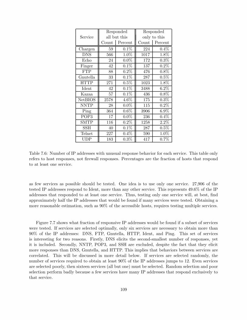
Responded RespondedService all but this only to this

Count Percent Count Percent

Chargen 59 0.1% 224 0.4%

DNS 566 1.0% 1017 1.8%

Echo 24 0.0% 172 0.3%

Finger 42 0.1% 137 0.2%

FTP 88 0.2% 476 0.8%

Gnutella 33 0.1% 287 0.5%

HTTP 271 0.5% 1023 1.8%

Ident 42 0.1% 3488 6.2%

Kazaa 57 0.1% 436 0.8%

NetBIOS 2578 4.6% 175 0.3%

NNTP 28 0.0% 115 0.2%

Ping 364 0.6% 3906 6.9%

POP3 17 0.0% 236 0.4%

SMTP 116 0.2% 1258 2.2%

SSH 40 0.1% 287 0.5%

Telnet 227 0.4% 590 1.0%

UDP 183 0.3% 417 0.7%

Table 7.6: Number of IP addresses with unusual response behavior for each service. This table onlyrefers to host responses, not firewall responses. Percentages are the fraction of hosts that respondto at least one service.

as few services as possible should be tested. One idea is to use only one service. 27,906 of thetested IP addresses respond to Ident, more than any other service. This represents 49.6% of the IPaddresses that responded to at least one service. Thus, testing only one service will, at best, findapproximately half the IP addresses that would be found if many services were tested. Obtaining amore reasonable estimation, such as 90% of the accessible hosts, requires testing multiple services.

Figure 7.7 shows what fraction of responsive IP addresses would be found if a subset of serviceswere tested. If services are selected optimally, only six services are necessary to obtain more than90% of the IP addresses: DNS, FTP, Gnutella, HTTP, Ident, and Ping. This set of servicesis interesting for two reasons. Firstly, DNS elicits the second-smallest number of responses, yetit is included. Secondly, NNTP, POP3, and SSH are excluded, despite the fact that they elicitmore responses than DNS, Gnutella, and HTTP. This implies that behaviors between services arecorrelated. This will be discussed in more detail below. If services are selected randomly, thenumber of services required to obtain at least 90% of the IP addresses jumps to 12. Even servicesare selected poorly, then sixteen services (all but one) must be selected. Random selection and poorselection perform badly because a few services have many IP addresses that respond exclusively tothat service.

109

0

20

40

60

80

100

2 4 6 8 10 12 14 16

Per

cent

age

of IP

Add

ress

es F

ound

Number of Services Tested

Percentage of IP Addresses Found by Testing Multiple Services

OptimalRandomPessimal

Figure 7.7: IP addresses found by using multiple services with optimal, random, and pessimalservice selection.

7.3.5 How is Firewall Behavior Correlated?

In order to quantify the correlation between firewall behavior, define the blocking correlation fromone service to another to be how much more likely, relatively, an IP addresses is to not respond toservice x given that it does not respond to service y. By formula, let Rx be the set of IP addressesresponding to the service x and R =

⋃

x Rx, the set of IP addresses that responded to at least oneservice. For firewall behavior correlation, what matters is the IP addresses for whom access to aservice are blocked. Thus, let Rx = R/Rx, the set of IP addresses that respond to at least oneservice, but not to service x. Then, the blocking correlation of a with b, C b

a, is given by:

Cba =

P [x ∈ Ra|x ∈ Rb] − P [x ∈ Ra]

1 − P [x ∈ Ra]=

‖R‖‖Ra ∪ Rb‖ − ‖Ra‖‖Rb‖

‖Rb‖‖Ra‖

A negative Cba would mean that it is more likely to respond to a if it does not respond to b. This

definition of correlation is closely related the correlation coefficient. In particular, the correlation

coefficient of responsiveness to two services a and b is√

CbaC

ab . Table 7.8 shows the correlation

between services. The bottom quartile is between 16% and 39%. The top quartile is between 66%and 89%.

High correlations reveal which services administrators consider equal, in terms of balance be-tween security risk and usefulness to remote users. The highest correlation is 89%. Chargen is89% correlated with Echo and Echo 89% correlated with Chargen. These services are often lumpedwith Discard, Daytime, and Time under the term “tiny services,” as they are simplistic services.Less correlation was expected, with Chargen blocked more often than Echo. However, this is notthe behavior: most IP addresses that respond to one service respond to the other. Interestingly,Finger is 89% correlated with NNTP, while NNTP is 80% correlated with Finger. That meansthat most IP addresses that respond to NNTP will also respond to Finger (although they may not

110

Service Letter A B C D E F G H I J K L M N O P Q

Chargen A x 34 89 77 69 77 41 61 74 33 78 40 68 60 69 72 48

DNS B 42 x 43 46 36 44 45 53 44 26 45 40 54 45 46 36 63

Echo C 89 35 x 80 72 81 42 63 76 34 81 42 69 61 71 69 50

Finger D 79 38 81 x 76 75 46 69 74 36 89 51 75 67 80 63 59

FTP E 49 20 51 53 x 48 34 35 49 20 62 21 50 49 66 49 35

Gnutella F 72 33 76 69 63 x 39 53 87 30 70 39 59 52 61 61 49

HTTP G 39 35 40 43 46 40 x 51 39 27 45 34 58 53 45 40 32

Ident H 39 28 40 44 31 36 34 x 36 25 42 26 51 42 42 30 27

Kazaa I 68 33 71 68 64 86 38 51 x 29 70 39 59 52 60 58 49

NetBIOS J 71 46 73 77 62 71 61 84 69 x 75 47 87 76 75 53 48

NNTP K 71 33 73 80 79 68 43 60 69 31 x 40 70 67 76 63 53

Ping L 29 23 30 36 21 30 25 29 30 16 32 x 29 24 31 23 37

POP3 M 58 37 59 63 61 54 52 68 55 34 66 35 x 78 69 48 42

SMTP N 50 30 51 55 57 46 46 54 47 29 62 28 75 x 64 46 37

SSH O 53 29 54 60 71 50 37 50 49 26 64 34 61 59 x 49 43

Telnet P 70 29 68 60 69 64 41 45 61 24 68 31 55 54 63 x 45

UDP Q 53 56 55 64 54 57 37 47 58 24 63 56 54 49 61 50 x

Table 7.8: Blocking correlation of IP addresses responding to two services, expressed as percentages.The upper-right value of 48 corresponds to CQ

A = 48%.

run either). Both NNTP and Finger are older, somewhat less popular services primarily run onUNIX-like operating systems, which may the cause of the high correlations.

Low correlations reflect administrators having dissimilar opinions about the security risk or(legitimate) usefulness to remote users. The lowest correlations are with NetBIOS. For example,Ping is 16% correlated with NetBIOS, the lowest correlation. This means that knowing that Pingwas blocked to an IP address did not make it much more likely that NetBIOS was blocked. Becausefew IP addresses were responsive to NetBIOS, the likely reason that the other services have lowcorrelations with NetBIOS is that NetBIOS is one of the first services blocked when configuringa firewall. In contrast, Ping is considered a relatively safe protocol to allow. Ignoring NetBIOS,the lowest correlations are between FTP and DNS and between FTP and Ping, at 20% and 21%respectively. This is partially a result of neither Ping nor DNS using TCP, which FTP and most ofthe services tested use. Indeed, many services have low correlations with Ping and DNS. However,UDP does not use TCP either, and FTP is only 35% correlated with UDP. This can be partiallyexplained by the fact that many firewalls having special configuration options for Ping and DNSpackets. However, that does not explain the mystery of why FTP is in both pairs. Although FTPhad many responses, Ident had more and SSH, SMTP, and POP3 all had only slightly fewer.

Besides NetBIOS, DNS had the second-smallest number of responders. It was expected thatDNS would have fewer listeners, but the small number of responders was unexpected. One theoryof why DNS rarely induces responses is that it uses UDP for transport (at least, as commonly usedand as tested), while most of the services tested employ TCP. Since TCP is connection-based, itis far simpler for firewalls to understand TCP communications than UDP communications. As a

111

Chargen

Echo

89

Finger

77

Gnutella

77

NNTP

78

89

80

81 81Kazaa

76

79

81

75 89

FTP

76 POP3

75

SSH

80

76

87 80

79 76

86

SMTP

78

NetBIOS

77

75 87

75

Ident

84

76

75

Figure 7.9: Blocking dependency digraph of firewall blocking. An arc service x to service y impliesthat Cy

x ≥ 75%.

result, UDP may be considered less secure than TCP. DNS’s behavior is not a function of simplynot using TCP, since Ping uses neither TCP nor UDP, and is the sixth-most responsive service.However, it may be a result of UDP itself. If the reason DNS is blocked is that it uses UDP, thanthe UDP service, which uses UDP, should be highly correlated with DNS. UDP is 56% correlatedwith DNS and DNS is 63% correlated with UDP. Although DNS is not as correlated with any otherservice, UDP is more heavily correlated with many other services, most notably Finger and NNTP.Thus, blocking UDP made it notably more likely to block DNS, the reverse is not true. Therefore,DNS is blocked for reasons beyond just being UDP.

These correlations imply a dependency, where it is more likely to block service x if service y isblocked. This can be represented by the blocking dependency digraph defined as follows: Let theset of nodes correspond to the set of services. Let there be an arc from x to y if C y

x ≥ 75%. Thus,an arc implies that an IP address is 75% less likely to respond to service x if it does not respond toservice y. Figure 7.9 shows the blocking dependency digraph, which has 30 arcs on twelve of theservices (nodes without arcs are excluded).

The cliques6 in the blocking dependency digraph show clusters of services that administratorshave similar opinions of. There are five completely connected cliques in this digraph. The largestone is Echo, Chargen, and Finger. These are less-common services that primarily run on UNIX-like operating systems. The second clique is Finger and NNTP. Again, both run on UNIX-likeoperating systems, but USENET, which is based on NNTP, remains somewhat popular, althoughnot as popular as it once was. Given the similarity of the reasons for these two cliques, it would

6Clique is normally used when discussing undirected graphs. For a directed graph, define a clique to be a maximalset of vertices which induce a complete digraph. Trivial cliques of one node are ignored.

112

be reasonable to expect Echo and Chargen to also be highly correlated with NNTP. Indeed, Echoand Chargen are highly correlated with NNTP, and NNTP is somewhat highly correlated withthem (71% and 73%), but not enough to be included in the digraph. Another clique is Kazaaand Gnutella, which is unsurprising given their similarity. A somewhat more surprising clique isPOP3 and SMTP, both e-mail protocols, albeit different in application: SMTP is used to sende-mails and POP3 is used to retrieve e-mails. This difference in applications means that SMTPis unauthenticated (generally) while POP3 requires authentication. Thus, one might expect thatadministrators would view their security requirements differently. However, most appear to not.The last clique is the most puzzling: Gnutella and Echo. One might expect Kazaa to also be inthis clique, given its close relationship with Gnutella, but Echo is only 71% correlated with Kazaa.The reasons for this clique are unclear.

Disconnected or weakly-connected nodes correspond to services with relatively unique profiles.Five services are missing from the digraph: DNS, HTTP, Ping, Telnet, and UDP. Three additionalservices have no outbound arcs: FTP, Ident, and SSH. These represent services that are blockedrelatively independently from other services. Ignoring UDP, which has no listeners, when servicesare ranked by the number of listening IP addresses, these services are seven of the top ten, includingthe top four. Thus, part of their low correlation comes from the fact that firewalls must be configuredto not block access from the Internet to public services running on hosts.

7.3.6 What Accessible Services do Hosts Run?

Table 7.4 shows the percentage of IP addresses that run each service as well as the estimated totalnumber of servers. Not surprisingly, Ping was the most common listening service, as it is the onlyservice which the operating system normally does the listening. Excluding Ping, HTTP, FTP,Telnet, and SMTP are the four next-most common. HTTP, FTP, and SMTP are the three basicservices of the Internet: file transfer, e-mail transfer, and web servers. The fourth most commonservice, Telnet, is vulnerable to password sniffer when used with encryption, which is the commonutilization. Telnet’s high listener count is somewhat concerning given the availability of a securealternative with more functionality, SSH.

The observant reader may wonder why the number of HTTP servers differs greatly fromNetcraft’s numbers[56]. This chapter estimates 16-17 million HTTP servers on the Internet, whileNetcraft’s number is 50 million. Netcraft’s number corresponds to the number of websites, not thenumber of HTTP servers. A single HTTP server can host million of web sites. A single web sitemay be hosted on dozens of HTTP servers. The net effect is the number of web sites is much largerthan the number of HTTP servers, at least on the Internet today.

7.3.7 How are Running Servers Correlated?

Although somewhat unrelated to the question of firewall behavior, another interesting question ishow often two services run on the same host. This requires looking at the correlation of IP addresseslistening to two service (the listening correlation). Table 7.10 shows the listening correlations ofthe services, where the listening correlation is defined akin to blocking correlation (let Lx be theset of IP addresses listening to a service):

LCba =

P [x ∈ La|x∈ Lb] − P [x ∈ La]

1 − P [x ∈ La]=

‖R‖‖La ∪ Lb‖ − ‖La‖‖Lb‖

‖Lb‖‖La‖

113

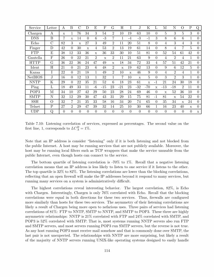
Service Letter A B C D E F G H I J K L M N O P Q

Chargen A x 1 76 34 3 54 2 10 19 63 10 0 5 3 5 3 0

DNS B 7 x 14 0 6 -3 7 1 -4 -3 -1 3 8 6 6 1 0

Echo C 82 3 x 27 3 49 2 11 20 51 8 0 4 3 4 3 0

Finger D 42 0 30 x 4 53 2 13 19 61 14 0 8 4 7 5 0

FTP E 38 12 33 36 x 36 33 30 10 51 81 0 52 54 61 42 0

Gnutella F 26 0 22 21 2 x 2 11 21 63 9 0 4 2 4 1 0

HTTP G 36 22 36 24 47 49 x 18 34 72 33 4 57 51 42 21 0

Ident H 21 0 21 23 6 48 2 x 19 62 13 0 9 6 12 5 0

Kazaa I 22 0 21 18 1 49 2 10 x 46 9 0 4 2 4 1 0

NetBIOS J 16 0 12 13 1 32 1 7 10 x 5 0 3 2 3 1 0

NNTP K 29 0 22 35 21 52 6 18 23 61 x -1 21 24 30 18 0

Ping L 18 49 33 11 -6 -15 23 -21 23 -32 -70 x -13 -18 2 11 0

POP3 M 34 10 27 42 29 50 23 28 24 69 46 0 x 52 36 10 0

SMTP N 32 12 29 30 47 43 31 29 15 75 81 -1 81 x 54 22 0

SSH O 32 7 21 35 33 58 16 34 20 74 65 0 35 34 x 24 0

Telnet P 27 2 29 47 39 32 14 25 10 30 66 1 16 23 40 x 0

UDP Q 0 0 0 0 0 0 0 0 0 0 0 0 0 0 0 0 x

Table 7.10: Listening correlation of services, expressed as percentages. The second value on thefirst line, 1, corresponds to LCB

A = 1%.

Note that an IP address is consider “listening” only if it is both listening and not blocked fromthe public Internet. A host may be running services that are not publicly available. Moreover, thehost may be running local filters such as TCP wrappers that make the service unusable from thepublic Internet, even though hosts can connect to the service.

The bottom quartile of listening correlation is -70% to 1%. Recall that a negative listeningcorrelation means that an IP address is less likely to listen to one service if it listens to the other.The top quartile is 32% to 82%. The listening correlations are lower than the blocking correlations,reflecting that an open firewall will make the IP addresses beyond it respond to many services, butrunning many services on a system is administratively difficult.

The highest correlations reveal interesting behavior. The largest correlation, 82%, is Echowith Chargen. Interestingly, Chargen is only 76% correlated with Echo. Recall that the blockingcorrelations were equal in both directions for these two services. Thus, firewalls are configuredmore similarly than hosts for these two services. The asymmetry of their listening correlations arelikely a result of Chargen being more open to nefarious uses. Three pairs of services had listeningcorrelations of 81%: FTP to NNTP, SMTP to NNTP, and SMTP to POP3. These three are highlyasymmetric relationships: NNTP is 21% correlated with FTP and 24% correlated with SMTP, andPOP3 is 52% correlated with SMTP. That is, most systems running NNTP servers also run FTPand SMTP servers, and most servers running POP3 run SMTP servers, but the reverse is not true.As any host running POP3 must receive mail somehow and that is commonly done over SMTP, thelast pair is not unexpected. The relationships with NNTP are more surprising, but likely a resultof the majority of NNTP servers running UNIX-like operating systems designed to easily handle

114

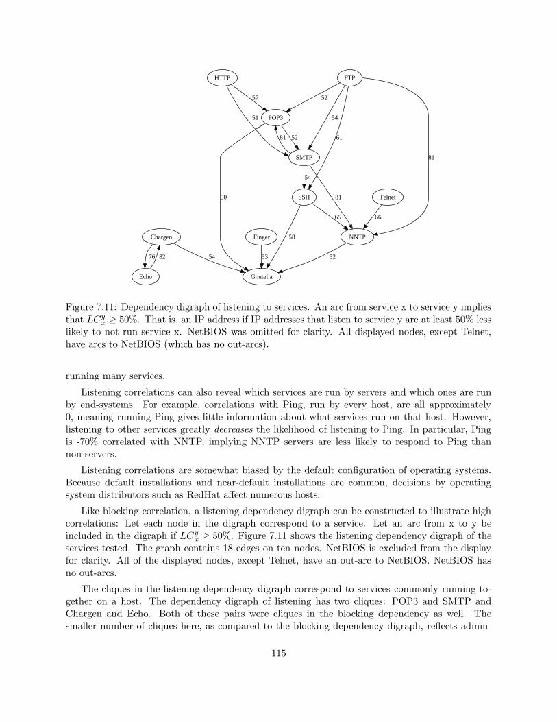
Chargen

Echo

76

Gnutella

5482

Finger

53

FTP

NNTP

81

POP3

52

SMTP

54

SSH

61

52

50

52

81

81

54

58

65

HTTP

57

51

Telnet

66

Figure 7.11: Dependency digraph of listening to services. An arc from service x to service y impliesthat LCy

x ≥ 50%. That is, an IP address if IP addresses that listen to service y are at least 50% lesslikely to not run service x. NetBIOS was omitted for clarity. All displayed nodes, except Telnet,have arcs to NetBIOS (which has no out-arcs).

running many services.

Listening correlations can also reveal which services are run by servers and which ones are runby end-systems. For example, correlations with Ping, run by every host, are all approximately0, meaning running Ping gives little information about what services run on that host. However,listening to other services greatly decreases the likelihood of listening to Ping. In particular, Pingis -70% correlated with NNTP, implying NNTP servers are less likely to respond to Ping thannon-servers.

Listening correlations are somewhat biased by the default configuration of operating systems.Because default installations and near-default installations are common, decisions by operatingsystem distributors such as RedHat affect numerous hosts.

Like blocking correlation, a listening dependency digraph can be constructed to illustrate highcorrelations: Let each node in the digraph correspond to a service. Let an arc from x to y beincluded in the digraph if LCy

x ≥ 50%. Figure 7.11 shows the listening dependency digraph of theservices tested. The graph contains 18 edges on ten nodes. NetBIOS is excluded from the displayfor clarity. All of the displayed nodes, except Telnet, have an out-arc to NetBIOS. NetBIOS hasno out-arcs.

The cliques in the listening dependency digraph correspond to services commonly running to-gether on a host. The dependency digraph of listening has two cliques: POP3 and SMTP andChargen and Echo. Both of these pairs were cliques in the blocking dependency as well. Thesmaller number of cliques here, as compared to the blocking dependency digraph, reflects admin-

115

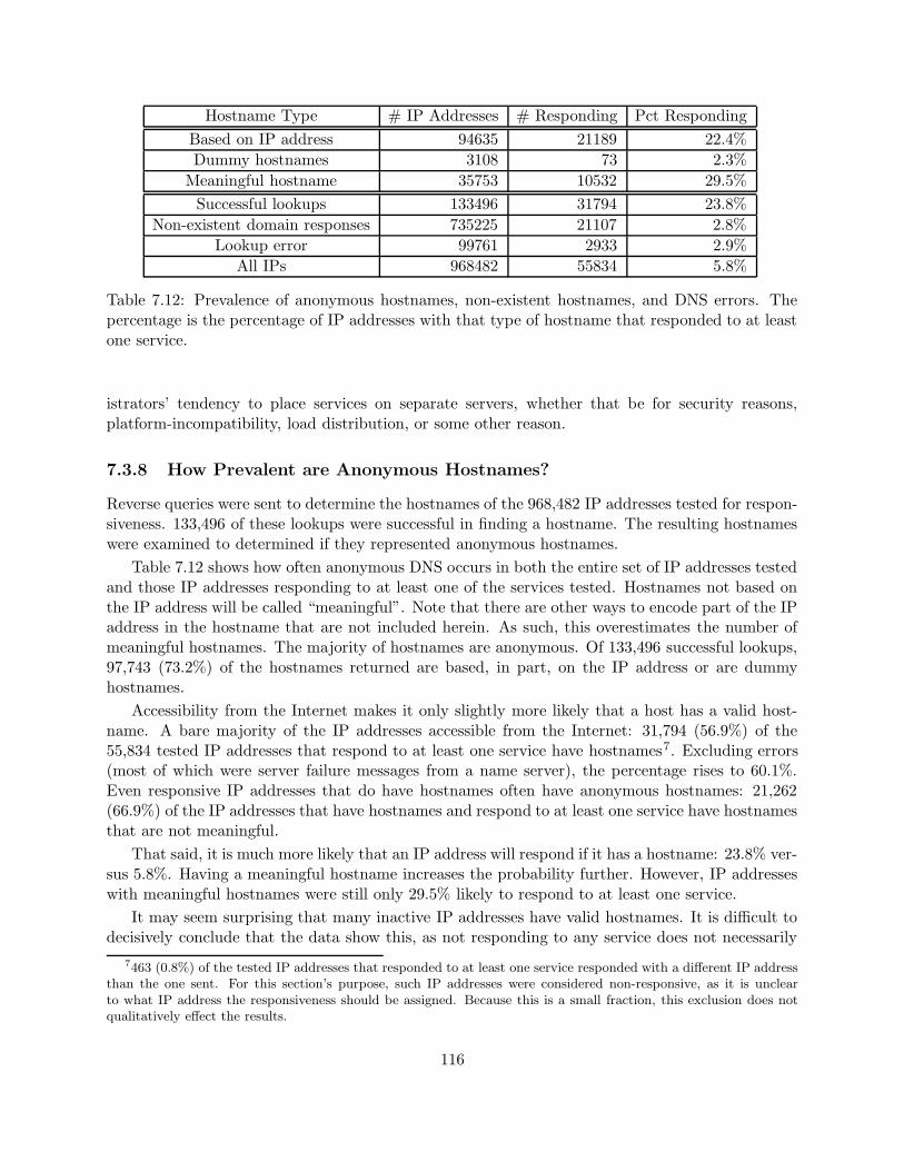
Hostname Type # IP Addresses # Responding Pct Responding

Based on IP address 94635 21189 22.4%

Dummy hostnames 3108 73 2.3%

Meaningful hostname 35753 10532 29.5%

Successful lookups 133496 31794 23.8%

Non-existent domain responses 735225 21107 2.8%

Lookup error 99761 2933 2.9%

All IPs 968482 55834 5.8%

Table 7.12: Prevalence of anonymous hostnames, non-existent hostnames, and DNS errors. Thepercentage is the percentage of IP addresses with that type of hostname that responded to at leastone service.

istrators’ tendency to place services on separate servers, whether that be for security reasons,platform-incompatibility, load distribution, or some other reason.

7.3.8 How Prevalent are Anonymous Hostnames?

Reverse queries were sent to determine the hostnames of the 968,482 IP addresses tested for respon-siveness. 133,496 of these lookups were successful in finding a hostname. The resulting hostnameswere examined to determined if they represented anonymous hostnames.

Table 7.12 shows how often anonymous DNS occurs in both the entire set of IP addresses testedand those IP addresses responding to at least one of the services tested. Hostnames not based onthe IP address will be called “meaningful”. Note that there are other ways to encode part of the IPaddress in the hostname that are not included herein. As such, this overestimates the number ofmeaningful hostnames. The majority of hostnames are anonymous. Of 133,496 successful lookups,97,743 (73.2%) of the hostnames returned are based, in part, on the IP address or are dummyhostnames.

Accessibility from the Internet makes it only slightly more likely that a host has a valid host-name. A bare majority of the IP addresses accessible from the Internet: 31,794 (56.9%) of the55,834 tested IP addresses that respond to at least one service have hostnames7. Excluding errors(most of which were server failure messages from a name server), the percentage rises to 60.1%.Even responsive IP addresses that do have hostnames often have anonymous hostnames: 21,262(66.9%) of the IP addresses that have hostnames and respond to at least one service have hostnamesthat are not meaningful.

That said, it is much more likely that an IP address will respond if it has a hostname: 23.8% ver-sus 5.8%. Having a meaningful hostname increases the probability further. However, IP addresseswith meaningful hostnames were still only 29.5% likely to respond to at least one service.

It may seem surprising that many inactive IP addresses have valid hostnames. It is difficult todecisively conclude that the data show this, as not responding to any service does not necessarily

7463 (0.8%) of the tested IP addresses that responded to at least one service responded with a different IP addressthan the one sent. For this section’s purpose, such IP addresses were considered non-responsive, as it is unclearto what IP address the responsiveness should be assigned. Because this is a small fraction, this exclusion does notqualitatively effect the results.

116

mean that the IP address is not active. The IP address may be beyond a firewall that blocks allinbound connection attempts. In fact, one would expect that a network which employs split DNSis more likely to be protected from the Internet by a restrictive firewall.

The data do show that more aggressive filtering of the input set based on ARIN data wouldhave skewed the responsiveness results. 141,969 of the DNS lookups fail with a non-existent domainresponse from ARIN, indicating that no DNS server is responsible for reverse queries on that IPaddress. Of these, 419 IP addresses were responsive. These IP addresses represent 58 differentassigned network blocks; none of them are within unassigned space. It is not clear why these IPaddresses do not have any DNS servers associated with their reverse lookup. Regardless, aggressivefiltering based on the top level domain database for in-addr.arpa would reduce the number of IPaddresses tested by only 14.7%, while causing testing to miss 0.7% of the responsive IP addresses.

7.4 Conclusions

This chapter presents a study of firewall configurations, firewall behaviors, and anonymous DNSon the Internet. It includes a methodology or such a study as well as an analysis of the results.

Most hosts on the Internet are behind a firewall. Specifically, this study showed that more than93% of the hosts on the Internet are behind a firewall or filtering device of some sort. Thus, almostevery packet delivered on the Internet passes through at least one such device. This makes givingan exact definition of “connected to the Internet” difficult at best.

This difficulty is reflected in looking at how many services must be examined to identify a largefraction of the IP addresses “connected to the Internet”. One of the goals of this study is to identifysuch IP addresses to compare against DNS census techniques. Although testing seventeen serviceswas expected to be somewhat overkill, it takes multiple services to find a large fraction of the IPaddresses that were found by the seventeen services tested. If services were selected randomly, itwould take twelve services to, with high probability, find at least 90% of the IP addresses. Evenif services were selected optimally, six services must be tested. If more services were added to theseventeen tested, these numbers would only increase further. Any similar attempt to look for mostof the IP addresses responsive from the Internet must test multiple services to obtain reasonableresult.

One unexpected result is the amount to which firewalls respond. Firewalls represent more than20% of the listeners for nine of the seventeen services tested and more than 20% of the respondersfor eight of the seventeen services tested. Clearly, any similar study of IP address behavior wouldalso need to detect and remove firewall responses to avoid large errors. This was somewhat expectedfor the Ident service, but large numbers of firewall responses are common to about half the servicestested.

Filtering devices differ in the level and type of filtering they employ. Approximately 56% of IPaddresses are protected by a firewall that blocks by default and 37% of IP addresses are behind afirewall that blocks by exception. In terms of security, blocking by exception is generally considereda worse policy, as it depends on knowing which services are bad. From a security standpoint, it ismuch better to assume by default that services are bad and only allow access to services on specifichosts where the service is useful enough to accept the security risk. The high percentage (37%) ofIP addresses behind a block-by-exception firewall raises a security concern.

117

Another interesting item to look at is how firewall behavior is correlated between services. Forsome pairs of services, such as Finger and NNTP, firewall behavior is heavily correlated. Highcorrelation between two services implies that the perceptions of the two services are similar. Insome cases, correlation is not symmetric: blocking A makes it more likely to block B, but notvice-versa. For example, not responding to POP3 makes it 87% less likely that an IP address willrespond to NetBIOS, but not responding to NetBIOS makes an IP address only 34% less likely torespond to to POP3. This behavior implies one of the services is perceived either as more riskyor less valuable. In this case, NetBIOS is both riskier and less valuable than POP3, in terms ofremote access.

Although not the primary motivation, the study naturally detects if hosts are listening to portsas well, if no filtering devices blocks the queries. 39% of hosts accessible from the Internet listen tono services, implying that a lot of hosts are accessible that likely do not need to be. Insecure servicescontinue to be prevalent, even when more secure alternatives exist. For example, Telnet is muchmore popular than SSH. There are approximately eleven million Telnet servers and approximatelyseven million SSH servers.

The services an IP address listens also exhibit correlated behavior. Unlike responding, wheremany hosts responded to almost all the services tested, few hosts listened to more than three orfour of the services. That does not mean, however, that there are not examples of highly correlatedbehavior. For example, most hosts than run either SMTP or POP3 run both. This relationship isalso not always symmetric. For example, listening to NNTP makes an IP address 81% more likelyto listen to FTP, while listening to FTP makes an IP address only 21% more likely to listen to FTP.When most servers running service A run some other service B, any security problem in service Bwill affect most A servers. In this case, if FTP servers could be compromised, then most NNTPservers are compromised as well. This leads to some unexpected security implications, where asecurity flaw in service B causes problems with A servers despite the fact that the services are notobviously related.

One of the goals of this study is to explore the accuracy of DNS methods of counting activeIP addresses. At first, DNS methods look good, as an IP address with a hostname is more thaneight times more likely to respond to an IP address without one. However, an IP address withan anonymous hostname is 24% less likely to respond than one with a meaningful name, and IPaddresses with dummy hostnames are less likely to respond than those without a hostname. Thatsaid, even IP addresses which are responsive on the Internet, which should be more likely to havehostnames, do not have a hostname 43.1% of the time. Assuming that every hostname, evenanonymous ones, corresponded to an actual host, DNS methods undercount the true number ofhosts by at least 15%.

This study leads to a new area of Internet measurement – a security study of the Internet,including how security defense mechanisms are deployed and configured on the Internet. Such astudy provides important information for vulnerability assessment and assists in designing newdefense mechanisms. Hopefully, this study will encourage new research and efforts in securitymeasurement. It is planned to continue to monitor how security-relevant behaviors on the Internetchange over time.

118

Chapter 8

Conclusions

The Internet has grown from four hosts in late 1969 to hundreds of millions of hosts today. Thisgrowth in size has been accompanied with a corresponding growth in importance to both scientificwork and economy activity. This thesis presented ways to measure and monitor today’s Internetto better understand its behavior and the behavior of those on it.

One basic piece of information to know about a network is its topology. Without knowing thehosts on a network and how they are connected, it is difficult to place other information aboutthe network in context. This thesis presented techniques used by an ongoing, long-term project tomeasure the topology of the Internet and how it changes over long time spans. Similar topologymeasurement techniques formed the basis of a venture capital-funded start-up that developed aproduct to measure the topologies of corporate networks, giving network administrators a snapshotof their topology. The combination of organic network growth and the decentralized nature of IPnetwork means that some corporations have a poor or limited feel for their network’s topology. Thetopology measurements can also provide insight on the effect of remote events. In the case of the1999 NATO bombing of Yugoslavia, it could detect when network elements were disrupted. Oneproblem with this technique is that it is difficult to determine which network elements should bemonitored. This problem is addressed by geolocation techniques.

One of the problems with topology measurements is that a host may be represented by multiplenodes under different IP aliases of the host. This thesis presented ways to resolve these IP aliases bydetermining the IP addresses belonging to a single host. Previous methods and implementationswere small-scale, designed to work on a few thousand IP addresses, and it was not known howeffective they were. Algorithms using the same basic techniques of previous work, but designed totest hundreds of thousands IP addresses, were presented and compared against previous methods.These algorithms were then run on approximately 400,000 IP addresses for their performance andaccuracy. Of the three techniques, the IPid technique performed best, but was expensive in termsof packets and time required. The UDP technique required few packets and ran quickly, but wasonly half as effective. The rate limit technique was almost as expensive as the IPid techniquebut performed worse than the UDP technique. However, each technique found IP aliasing notfound by the other two techniques. Thus, applications with tight time constraints should use UDP,applications with looser time constraints should use UDP and IPid, and applications requiring highaccuracy must use all three.

The Internet is, at its heart, a set of interconnected hosts that forward packets. Routing

119

is the process of deciding how those hosts should forward packets. Routing is multilevel andcompartmentalized, making global measurements difficult. The parallel traceroutes done to measurethe Internet’s topology give routing information for many destinations, but measure the routingdecisions made for each destination at only a few routers. This gives an incoherent set of routingdecisions that is difficult to analyze. This thesis proposed a new way to measure these routingdecisions by attempting to determine the inbound paths to a particular destination. Althoughsome techniques to measure inbound paths do exist, they yield minimal information. The proposedtechnique measures more than sixty times the number of routing decisions measured by previoustechniques, at the cost of being less accurate.

One problem facing the Internet is denial-of-service attacks. Because packets are forwardedalmost purely based on the destination, the true source of a packet need not be the source listedin the packet unless the source wants to receive replies. In an attack, the goal is to disrupt service,which, quite often, does not require receiving replies. Thus, the attacker can forge (“spoof”) thesource of the attack packets. This thesis described a scheme to find the source of an attackingstream of packets. This controversial scheme uses some of the same denial-of-service techniquesused by attackers. Although not ideal and not designed for multiple attack streams, which havebecome popular, it is designed for the current Internet. Other, more desirable techniques thatrequire altering the Internet were presented, leading to much later work on defeating or locatingdenial-of-service attacks.

Another problem facing network operators is ensuring that their networks are operating prop-erly. One aspect of this is monitoring link and end-to-end delays. This can obviously be done byplacing measurement hosts next to each router, but that is expensive and difficult to maintain.This thesis described RCM, a delay measurement and path monitoring system that requires only asingle measurement. RCM uses tunnels to create virtual measurement hosts next to routers. Thismeans RCM is cheaper, faster, and easier to deploy and maintain. RCM uses a novel networktomography technique to determine link delays from the measured delays. RCM’s network tomog-raphy technique requires few probes per path, does not need to address internal routers, does notrequire hosts at every router, is able to model asymmetric networks, and can distinguish betweenpropagation and queue delays. RCM is implemented and operational on an AT&T’s network. Forthat network, RCM determines link delays that match network configuration information withoutRCM knowing the information.

Firewalls and filtering devices have become common on the Internet. It is unclear exactly howprevalent filtering devices are or how many packet are filtered. This thesis presented a large-scaleanalysis of filtering. One surprising result is that at least 93% of the IP addresses are behind afiltering device of some sort, meaning that almost every network communication must pass througha filter. The exact level of filtering varies by service, with filtering of two different services beinghighly dependent, especially when those services are similar.

Firewalls and filtering devices have the effect of separating the Internet. The naming system isalso often separated, with IP addresses resolving to different hostnames within and without localnetworks. This thesis presented the results from an examination of the hostnames of almost amillion IP addresses. 73% of hostnames are determined from the IP address or are dummy names.Since IP-derived hostnames are commonly created for every IP address on a network without regardto whether or not there is a host at the IP address, hostnames are a poor indication of the existenceof a host. Thus, the prevalence of IP-derived hostnames implies that host-count techniques basedon DNS are inaccurate. Even if every IP address with a DNS hostname corresponded to an actual

120

host, 15% of IP addresses which respond from the Internet do not have a hostname, and wouldtherefore be incorrectly counted as inactive by DNS-based host-counting techniques.

This thesis presented ways to measure and monitor multiple aspects of today’s Internet. Itincludes analysis of the accuracy of the presented measurement techniques, as well as experimentalresults from those measurement system on the Internet. Being able to measure the current Internetmeans that the Internet can be better understood, including its limitations and deficiencies. Hope-fully, this will lead to improved network design, network protocols, and network performance.

121

122

Bibliography

[1] M. Adler. Tradeoffs in probabilistic packet morking for IP traceback. In Proceedings of 2002Symposium on Theorem of Computing, 2002.

[2] L. Bain and M. Engelhardt. Introduction to Probability and Mathematical Statistics. PWS-Kent Publishing Company, 1991.

[3] P. Barford, A. Bestavros, J. Byers, and M. Crovella. On the marginal utility of networktopology measurements. In ACM SIGCOMM Internet Measurement Workshop 2001, Nov.2001.

[4] S. Bellovin. A technique for counting NATted hosts. In ACM SIGCOMM Internet Measure-ment Workshop 2002, Nov. 2002.

[5] Y. Breitbart, C. Y. Chan, M. N. Garofalakis, R. Rastogi, and A. Silberschatz. Efficientlymonitoring bandwidth and latency in IP networks. In INFOCOM, pages 933–942, 2001.

[6] H. Burch. Eliminating machine duplicity in traceroute-based internet topology measurements.Technical Report CMU-CS-02-146, CMU, May 2002.

[7] H. Burch and W. Cheswick. Mapping the Internet. IEEE Computer, 32(4), Apr 1999.

[8] H. Burch and W. Cheswick. Tracing anonymous packets to their source by selective denial-of-service probes. In USENIX Lisa, 2000.

[9] H. Burch and D. Song. A security study of the Internet: An analysis of firewall behavior andanonymous DNS. Technical Report CMU-CS-04-141, CMU, July 2004.

[10] Catrography. National Geographic, Jan 2000.

[11] J. D. Case, M. Fedor, M. L. Shoffstall, and C. Davin. Simple network management protocol.RFC 1157, May. 1990.

[12] CERT. Tcp syn flooding and ip spoofing attacks. CERT advisory CA-96.21, Sept 1996.

[13] CERT. smurf ip denial-of-service attacks. CERT advisory CA-98.01, Jan 1998.

[14] CERT. Results of the distributed-systems intruder tools workshop. The CERT CoordinationCenter, Dec 1999.

[15] B. Cheswick. The design of a secure Internet gateway. In USENIX Summer Conference,pages 233–237, Anaheim, California, 1990.

123

[16] W. Cheswick and H. Burch. http://research.lumeta.com/ches/map/movie.mpeg.

[17] W. Cheswick, H. Burch, and S. Branigan. Mapping and visualizing the Internet. In Proceed-ings of 2000 USENIX Annual Technical Conference, June 2000.

[18] W. Cheswick, H. Burch, S. Branigan, and F. Wojcik. Internet mapping project. http://re-search.lumeta.com/ches/map/index.html.

[19] W. Cheswick, J. Nonnenmacher, C. Sahinalp, R. Sinha, and K. Varadhan. Modeling Internettopology. Technical Report 113410-991116-18TM, Lucent Technologies, 1999.

[20] Cisco Technology. http://www.internetindicators.com.

[21] K. Claffy. private communication.

[22] R. Clements. Who talks ICMP, too? – survey of 18 february 83. RFC 844, Feb. 1983.

[23] M. Coates and R. Nowak. Network tomography for internal delay estimation. In IEEEInternational Conference on Acoustics, Speech and Signal Processing, 2001.

[24] J. Cohen. Drawing graphs to convery proximity: an incremental arrangement method. ACMTransactions on Human-Computer Interaction, 4(3):197–229, 1997.

[25] Cypergeography. http://www.cybergeography.org/.

[26] D. Dean, M. Franklin, and A. Stubblefield. An algebraic approach to IP traceback. ACMTransactions of Information and System Security, 5(2):119–137, May 2001.

[27] S. Deering and R. Hinden. Internet protoc,l version 6 (IPv6). RFC 2460, Dec. 1998.

[28] D. W. Dodds. August, 1974, survey of new-protocol telnet servers. RFC 701, Aug. 1974.

[29] D. W. Dodds. November, 1974, survey of new-protocol telnet servers. RFC 669, Dec. 1974.

[30] D. W. Dodds. September, 1974, survey of new-protocol telnet servers. RFC 702, Sep. 1974.

[31] D. W. Dodds. February, 1975, survey of new-protocol telnet servers. RFC 679, Feb. 1975.

[32] D. W. Dodds. July, 1975, survey of new-protocol telnet servers. RFC 703, Jul. 1975.

[33] T. Doeppner, P. Klein, and A. Koyfman. Using rotuer stamping to identify the source of IPpackets. In CCS ’00, 2000.

[34] N. Duffield. Simple network performance tomography. In ACM SIGCOMM Internet Mea-surement Conference, Oct 2003.

[35] P. Eades. A heuristic for graph drawing. Congressus Numerantium, 42:149–160, 1984.

[36] D. Farinacci, T. Li, S. Hanks, D. Meyer, and P. Traina. Generic routing encapsulation (GRE).RFC 2784, Mar. 2000.

[37] P. Ferguson and D. Senie. Network ingress filtering: Defeating denial of service attacks whichemploy ip source address spoofing. RFC 2667, Jan 1998.

124

[38] R. Fielding, J. Gettys, J. Mogul, H. Frystk, L. Masinter, P. Leach, and T. Berners-Lee.Hypetertext transfer protocol – HTTP/1.1. RFC 2616, Jun. 1999.

[39] A. Frick, A. Ludwig, and H. Mehldau. A fast adaptive layout algorithm for undirected graphs.In Proceedings of Graph Drawing ’94, 1995.

[40] Gnutella. http://gnutella.wega.com.

[41] R. Govindan and V. Paxson. Estimating routing ICMP generation times. In Proceedings ofthe Workshop on Passive and Active Measurements, March 2002.

[42] R. Govindan and H. Tangmunarunkit. Heuristics for Internet map discovery. In INFOCOM(3), pages 1371–1380, 2000.

[43] N. W. G. in DARPA, Internet Activities Board, End-to End Services Task Force. Protocolstandard for a NetBIOS service on a TCP/UDP transport: Concepts and methods. RFC1001, Mar. 1987.

[44] IP Route Analytics, Packet Design. http://www.route-explorer.com/.

[45] ISC. ISC internet domain survey. http://www.isc.org/index.pl?/ops/ds/, 1998 - 2004.

[46] V. Jacobson. traceroute. ftp://ftp.ee.lbl.gov/traceroute.tar.Z, 1989.

[47] C. Jin, H. Wang, and K. Shin. Hop-count filtering: An effective defense against spoofedDDoS traffic. In CCS ’03, 2003.

[48] M. S. Johns. Identification protocol. RFC 1413, Feb. 1993.

[49] B. Kantor and P. Lapsley. Network news transfer protocol. RFC 977, Feb. 1986.

[50] Kazaa. http://www.kazaa.com.

[51] T. Kernen. traceroute.org. http://www.traceroute.org.

[52] K. Keys. iffinder. http://www.caida.org/tools/measurement/iffinder/, 2000.

[53] J. Klensin. Simple mail transfer protocol. RFC 2821, Apr. 2001.

[54] T. Kohno, A. Broide, and kc claffy. Remote physical device fingerprinting. In Proceedings ofIEEE Symposium on Security and Privacy, March 2005.

[55] P. D. Lebling. Survey of FTP mail and MLFL. RFC 751, Dec. 1978.

[56] N. LTD. Netcraft web server survey. http://www.netcraft.com.

[57] Lumeta Corporation. Internet mapping project. http://www.lumeta.com/mapping.html.

[58] Lumeta Corporation. http://www.lumeta.com/.

[59] B. Lyon. The opte project. http://www.opte.org/.

125

[60] R. Mahajan, S. M. Bellovin, S. Floyd, J. Ioannidis, V. Paxson, and S. Shenker. Controllinghigh bandwidth aggregates in the network. Computer Communications Review, 32(3):62–73,Jul 2002.

[61] D. McRobb, K. Claffy, and T. Monk. Skitter: CAIDA’s macroscopic Internet topologydiscovery and tracking tool. http://www.caida.org/tools/skitter/, 1999.

[62] Merit Networks. Routing assets database. http://www.radb.net/.

[63] MIDS. http://www.mids.org/.

[64] P. Mockapetris. Domain names – implementation and specification. RFC 1035, Nov. 1987.

[65] J. Moy. OSPF version 2. RFC 2328, Apr. 1998.

[66] T. Munzner. H3viewer. http://graphics.stanford.edu/˜munzner/h3/.

[67] T. Munzner. H3: Laying out large directed graphs in 3d hyperbolic space. In Proc. of 1997IEEE Symposium on Information Visualization, pages 2–10, October 20–21 1997.

[68] J. Myers and M. Rose. Post office protocol - version 3. RFC 1939, May. 1996.

[69] Netsizer. http://www.netsizer.com, 2000.

[70] J. Pansiot and D. Grad. On routes and multicast trees in the Internet. ACM ComputerCommunication Review, 28(1):41–50, Jan. 1998.

[71] K. Park and H. Lee. On the effectiveness of probabilistic packet marking for IP tracebackunder denial of service attack. In IEEE INFOCOM 2001, pages 338–347, 2001.

[72] V. Paxson. End-to-end routing behavior in the Internet. IEEE/ACM Transactions on Net-working, 5(5):601–615, 1997.

[73] Peacock Maps. http://www.peacockmaps.com.

[74] J. Postel. User datagram protocol. RFC 768, Aug. 1980.

[75] J. Postel. Internet control message protocol. RFC 792, Sept. 1981.

[76] J. Postel. Internet Protocol. RFC 791, Sept. 1981.

[77] J. Postel. Character generator protocol. RFC 864, May 1983.

[78] J. Postel. Echo protocol. RFC 862, May. 1983.

[79] J. Postel. Telnet protocol specification. RFC 854, May. 1983.

[80] J. Postel. File transfer protocol. RFC 959, Oct. 1985.

[81] T. F. Project. Freebsd v5.3. http://www.freebsd.org/, Nov. 2004.

[82] N. Provos and P. Honeyman. Scanssh - scanning the internet for ssh servers. UMich TechnicalReport CITI-TR-01-13, Oct. 2001.

126

[83] RIPE. Ripe region hostcount. http://www.ripe.net/ripencc/pub-services/stats/hostcount/-index.html.

[84] E. Rosen and Y. Rekhter. BGP/MPLS VPNs. RFC 2547, Mar. 1999.

[85] RouteDynamics, Ipsum Networks. http://www.ipsumnetworks.com/.

[86] S. Russel and P. Norvig. Artificial Intelligence: A Modern Approach. Prentice-Hall, 1994.

[87] S. Savage, D. Wetherall, A. R. Karlin, and T. Anderson. Practical network support for IPtraceback. In SIGCOMM, pages 295–306, 2000.

[88] A. Shaikh and A. Greenberg. OSPF monitoring: Architecture, design and deployment ex-perience. In USENIX Symposium on Networked System Design and Implementation, Mar2004.

[89] Y. Shavitt, X. Sun, A. Wool, and B. Yener. Computing the unmeasured: An algebraicapproach to Internet mapping. Technical Report 2000-15, DIMACS, 23 2000.

[90] J. Shewchuck. An introduction to the conjugate gradient method without the agonizing pain.unpublished paper.

[91] M. F. Shih and A. O. Hero. Unicast inference of network link delay distributions from edgemeasurements. In IEEE International Conference on Acoustics, Speech and Signal Processing,May 2001.

[92] D. Smallberg. Survey of smtp implementations. RFC 876, Sep. 1983.

[93] D. Song and A. Perrig. Advanced and authenticated marking schemes for IP traceback. InIEEE INFOCOM 2001, pages 878–886, 2001.

[94] N. Spring, R. Mahajan, and D. Wetherall. Measuring ISP topologies with Rocketfuel. InACM SIGCOMM 2002, Aug. 2002.

[95] R. Teixeira, K. Marzullo, S. Savage, and G. Voelker. In search of path diversity in ispnetworks. In ACM SIGCOMM Internet Measurement Conference 2003, Nov. 2003.

[96] I. G. Tollis, G. D. Battista, R. Tamassia, P. Eades, and G. D. Battista. Graph Drawing.Prentice-Hall, 1999.

[97] W. Townsley, A. Valencia, A. Rubens, G. Pall, G. Zorn, and B. Palter. Layer two tunnelingprotocol “L2TP”. RFC 2661, Aug. 1999.

[98] L. Trefethen and D. B. III. Numerical Linear Algebra. SIAM, 1997.

[99] Y. Tsang, M. Yildiz, P. Barford, and R. Nowak. Network radar: Tomography from roundtrip time measurements. In IMC’04, pages 175–180, Oct. 2004.

[100] D. Tunkelange. Jiggle: Java interactive graph layout environment. In Proceedings of GraphDrawing ’98, 1998.

127

[101] J. Vardi. Network tomography: Estimating source-destination traffic intensities from linkdata. J. of the American Statistical Association, pages 365–377, 1996.

[102] W. Venema. TCP wrapper: Network monitoring, access control, and booby traps. In Pro-ceedings of the 3rd UNIX Security Symposium, pages 85–92, Sept. 1999.

[103] W. Wei, B. Wang, D. Towsley, and J. Kurose. Model-based identification of dominant con-gested links. In ACM Internet Measurement Conference, 2003.

[104] A. Westine, D. Smallberg, and J. Postel. Summary of smallberg surveys. RFC 847, Feb.1983.

[105] Wired, Dec 1998.

[106] A. Yaar, A. Perrig, and D. Song. Pi: A path identification mechanism to defend againstDDoS attacks. In Proceedings of the 2003 IEEE Symposium on Security and Privacy, 2003.

[107] T. Ylonen. Secure login connections over the internet. In Proceedings of 6th USENIX SecuritySymposium, pages 37–42, Jul. 1996.

[108] B. Ziegler. Hacker tangles Panix web site. Wall Street Journal, September 12 1996.

[109] D. Zimmerman. The finger user information protocol. RFC 1288, Dec. 1991.

128